convolutional neural networks for steady flow approximation · lutional neural networks (cnns). we...
TRANSCRIPT
Convolutional Neural Networksfor Steady Flow Approximation
Xiaoxiao GuoUniversity of Michigan
Wei LiAutodesk Research
Francesco IorioAutodesk Research
ABSTRACTIn aerodynamics related design, analysis and optimizationproblems, flow fields are simulated using computational fluiddynamics (CFD) solvers. However, CFD simulation is usu-ally a computationally expensive, memory demanding andtime consuming iterative process. These drawbacks of CFDlimit opportunities for design space exploration and forbidinteractive design. We propose a general and flexible ap-proximation model for real-time prediction of non-uniformsteady laminar flow in a 2D or 3D domain based on convo-lutional neural networks (CNNs). We explored alternativesfor the geometry representation and the network architec-ture of CNNs. We show that convolutional neural networkscan estimate the velocity field two orders of magnitude fasterthan a GPU-accelerated CFD solver and four orders of mag-nitude faster than a CPU-based CFD solver at a cost of a lowerror rate. This approach can provide immediate feedbackfor real-time design iterations at the early stage of design.Compared with existing approximation models in the aero-dynamics domain, CNNs enable an efficient estimation forthe entire velocity field. Furthermore, designers and engi-neers can directly apply the CNN approximation model intheir design space exploration algorithms without trainingextra lower-dimensional surrogate models.
KeywordsConvolutional Neural Networks; Surrogate Models; Compu-tational Fluid Dynamics; Machine Learning
1. INTRODUCTIONComputational fluid dynamics (CFD) analysis performs
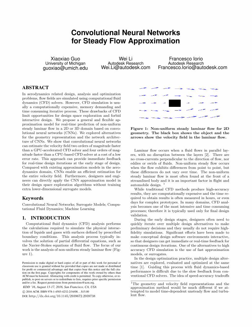
the calculations required to simulate the physical interac-tion of liquids and gases with surfaces defined by prescribedboundary conditions. This analysis process typically in-volves the solution of partial differential equations, such asthe Navier-Stokes equations of fluid flow. The focus of ourwork is the analysis of non-uniform steady laminar flow (Fig-ure 1).
Permission to make digital or hard copies of all or part of this work for personal orclassroom use is granted without fee provided that copies are not made or distributedfor profit or commercial advantage and that copies bear this notice and the full cita-tion on the first page. Copyrights for components of this work owned by others thanACM must be honored. Abstracting with credit is permitted. To copy otherwise, or re-publish, to post on servers or to redistribute to lists, requires prior specific permissionand/or a fee. Request permissions from [email protected].
KDD ’16, August 13-17, 2016, San Francisco, CA, USAc© 2016 ACM. ISBN 978-1-4503-4232-2/16/08. . . $15.00
DOI: http://dx.doi.org/10.1145/2939672.2939738
Figure 1: Non-uniform steady laminar flow for 2Dgeometry. The black box shows the object and thearrows show the velocity field in the laminar flow.
Laminar flow occurs when a fluid flows in parallel lay-ers, with no disruption between the layers [2]. There areno cross-currents perpendicular to the direction of flow, noreddies or swirls of fluids. Non-uniform steady flow occurswhen the flow exhibits differences from point to point, butthese differences do not vary over time. The non-uniformsteady laminar flow is most often found at the front of astreamlined body and it is an important factor in flight andautomobile design. 1
While traditional CFD methods produce high-accuracyresults, they are computationally expensive and the time re-quired to obtain results is often measured in hours, or evendays for complex prototypes. In many domains, CFD anal-ysis becomes one of the most intensive and time consumingprocesses; therefore it is typically used only for final designvalidation.
During the early design stages, designers often need toquickly iterate over multiple design alternatives to makepreliminary decisions and they usually do not require high-fidelity simulations. Significant efforts have been made tomake conceptual design software environments interactive,so that designers can get immediate or real-time feedback forcontinuous design iterations. One of the alternatives to highaccuracy CFD simulation is the use of fast approximationmodels, or surrogates.
In the design optimization practice, multiple design alter-natives are explored, evaluated and optimized at the sametime [1]. Guiding this process with fluid dynamics-basedperformance is difficult due to the slow feedback from con-ventional CFD solvers. The idea of speed-accuracy tradeoffs
1The geometry and velocity field representations and theapproximation method would be much different if we at-tempted to model time-dependent unsteady flow and turbu-lent flow.
[6] also leads to practical design space exploration and de-sign optimization in the aerodynamics domain by using fastsurrogate models.
Data-driven surrogate models become more and more prac-tical and important because many design, analysis and op-timization processes generate high volume CFD physical orsimulation data. Over the past years, deep learning ap-proaches (see [5, 26] for survey) have shown great successesin learning representations from data, where features arelearned end-to-end in a compositional hierarchy. This isin contrast to the traditional approach which requires thehand-crafting of features by domain experts. For data thathave strong spatial and/or temporal dependencies, Convo-lutional Neural Networks (CNNs) [20] have been shown tolearn invariant high-level features that are informative forsupervised tasks.
In particular, we propose a general CNN-based approxi-mation model for predicting the velocity field in 2D or 3Dnon-uniform steady laminar flow. We show that CNN basedsurrogate models can estimate the velocity field two ordersof magnitude faster than a GPU-accelerated CFD solveror four orders of magnitude faster than a CPU-based CFDsolver at a cost of a low error rate. Another benefit of usinga CNN-based surrogate model is that we can collect trainingdata from either physical or simulation results. The knowl-edge of fluid dynamics behavior can then be extracted fromdata sets generated by different CFD solvers, using differentsolution methods. Traditional high accuracy simulation isstill an important step to validate the final design, but fastCFD approximation models have wide applications in theconceptual design and the design optimization process.
2. RELATED WORK
2.1 CFD AnalysisComputational methods have emerged as powerful tech-
niques for exploring physical and chemical phenomena andfor solving real engineering problems. In traditional CFDmethods, Navier-Stokes equations solve mass, momentumand energy conservation equations on discrete nodes (thefinite difference method, FDM) [11], elements (the finite el-ement method, FEM) [29], or volumes (the finite volumemethod, FVM) [24]. In other words, the nonlinear partialdifferential equations are converted into a set of non-linearalgebraic equations, which are solved iteratively. TraditionalCFD simulation suffers from long response time, predomi-nantly because of the complexity of the underlying physicsand the historical focus on accuracy.
The Lattice Boltzmann Method (LBM) [22] was intro-duced to overcome the drawbacks of the lattice gas cellularautomata. In LBM, the fluid is replaced by fractious parti-cles. These particles stream along given directions (latticelinks) and collide at the lattice sites. LBM can be consid-ered as an explicit physical-based approximation method.The collision and streaming processes are local [23]. LBMemerged as an alternative powerful method for solving fluiddynamics problems, due to its ability to operate with com-plex geometry shapes and to its trivially parallel implemen-tation nature [31, 21]. Since distinct particle motion canbe decomposed over many processor cores or other hard-ware units, efficient implementations on parallel computersare relatively easy. LBM can also handle complex boundaryconditions. However, LBM still requires numerous iterations
and its convergence speed depends on the geometry bound-aries. In this paper, we use LBM to generate all the trainingdata for the CNNs, and we compare the speed of our CNNbased surrogate models with both traditional CPU LBMsolvers and GPU-accelerated LBM solvers.
Compared with physical-based simulation and approxima-tion methods, our approach falls into the category of data-driven surrogate models (or supervised learning in machinelearning). The knowledge of fluid dynamics behavior can beextracted from large data sets of simulation data by learningthe relationship between an input feature vector extractedfrom geometry and the ground truth data output from a fullCFD simulation. Then, without the computationally expen-sive iterations that a CFD solver requires to allow the flowto converge to its steady state, we can directly predict thesteady flow behavior in a fraction of the time. The number ofiterations and runtime in a CFD solver is usually dependenton the complexity of geometries and boundary conditions,but they are irrelevant to those factors in the predictionprocess. Note that only the prediction runtime of surrogatemodels has a significant impact on the design processes. Thetraining time of the surrogate models is irrelevant.
2.2 Surrogate Modeling in CFD-based DesignOptimization
The role of design optimization has been rapidly increas-ing and evolving in aerodynamics related fields, such asaerospace and architecture design [1]. CFD solvers havebeen widely used in design optimization (finding the bestdesign parameters that satisfy project requirements) and de-sign space exploration (finding multiple designs that satisfythe requirements). However, the direct application of a CFDsolver in design optimization is usually computationally ex-pensive, memory demanding and time consuming. The ba-sic idea of using surrogates (approximation models) is toreplace a high-accuracy, expensive analysis process with aless expensive approximation. CFD surrogate models can beconstructed from physical experiments [30]. However, high-fidelity numerical simulation proves to be reliable, flexible,and relatively cheap compared with physical experiments(see [1] and references therein).
Various surrogate models have been explored for designprocesses, such as polynomial regression [12, 3], multipleadaptive regression splines (MARS) [10], Kriging [12, 16],radial basis function network [19], and artificial neural net-works [7, 4]. The existing approaches only predict a re-stricted subset of the whole CFD velocity field. For ex-ample, predict the pressure on a set of points on an ob-ject surface [32]. Most existing approaches also depend ondomain-specific geometry representations and can only beapplied to low-order nonlinear problems or small scale ap-plications [10, 18]. The models are usually constructed bymodeling the response of a simulator on a limited numberof intelligently chosen data points. Instead of modeling eachindividual low-dimensional design problem, we model thegeneral non-uniform steady laminar CFD analysis solution,so that our model can be reused in multiple different, lower-dimensional optimization processes, and predict the wholevelocity field.
2.3 Convolutional Neural NetworksConvolutional neural networks have been proven success-
ful in learning geometry representations [27, 13]. CNNs
also enable per-pixel predictions in images. For example,FlowNet [8] predicts the optical flow field from a pair of im-ages. Eigen, Puhrsch and Fergus [9] estimate depth from asingle image. Recently, CNNs are applied on voxel to voxelprediction problems, such as video coloring [28].
Our approach applies CNNs to model large-scale non-linear general CFD analysis for a restricted class of flowconditions. Our method obtains a surrogate model of thegeneral high-dimensional CFD analysis of arbitrary geom-etry immersed in a flow for a class of flow conditions, andnot a model based on predetermined low-dimensional inputs.For this reason, our model subsumes a multitude of lower-dimensional models, as it only requires training once and canbe interrogated by mapping lower-dimensional problems intoits high-dimensional input space. The main contribution ofour CNN based CFD prediction is to achieve up to two tofour orders of magnitude speedup compared to traditionalLattice Boltzmann Method (LBM) for CFD analysis at acost of low error rates.
3. CONVOLUTIONAL NEURAL NETWORKSURROGATE MODELS FOR CFD
We propose a computational fluid dynamics surrogate modelbased on deep convolutional neural networks (CNNs). CNNshave been proven successful in geometry representation learn-ing and per-pixel prediction in images. The other motivationof adopting CNNs is its memory efficiency. Memory require-ment is a bottleneck to build whole velocity field surrogatemodels for large geometry shapes. The sparse connectiv-ity and weight-sharing property of CNNs reduce the GPUmemory cost greatly.
Our surrogate models have three key components. First,we adopt signed distance functions as a flexible and generalgeometric representation for convolutional neural networks.Second, we use multiple convolutional encoding layers to ex-tract abstract and high-level geometric representations. Fi-nally, there are multiple convolutional decoding layers thatmap the abstract geometric representations into the compu-tational fluid dynamics velocity field.
In the rest of this section, we describe the key componentsin turn.
3.1 Geometry RepresentationGeometry can be represented in multiple ways, such as
boundaries and geometric parameters. However, those rep-resentations are not effective for neural networks since thevectors’ semantic meaning varies. In this paper, we use aSigned Distance Function (SDF) sampled on a Cartesiangrid as the geometry representation. SDF provides a univer-sal representation for different geometry shapes and worksefficiently with neural networks.
Given a discrete representation of a 2D geometry on aCartesian grid, in order to compute the signed distance func-tion, we first create the zero level set, which is a set of points(i, j) that give the geometry boundary (surface) in a domainΩ ⊂ R2:
Z =
(i, j) ∈ R2 : f(i, j) = 0
(1)
where f is the level set function s.t. f(i, j) = 0 if and onlyif (i, j) is on the geometry boundary, f(i, j) < 0 if and onlyif (i, j) is inside the geometry and f(i, j) > 0 if and only if(i, j) is outside the geometry.
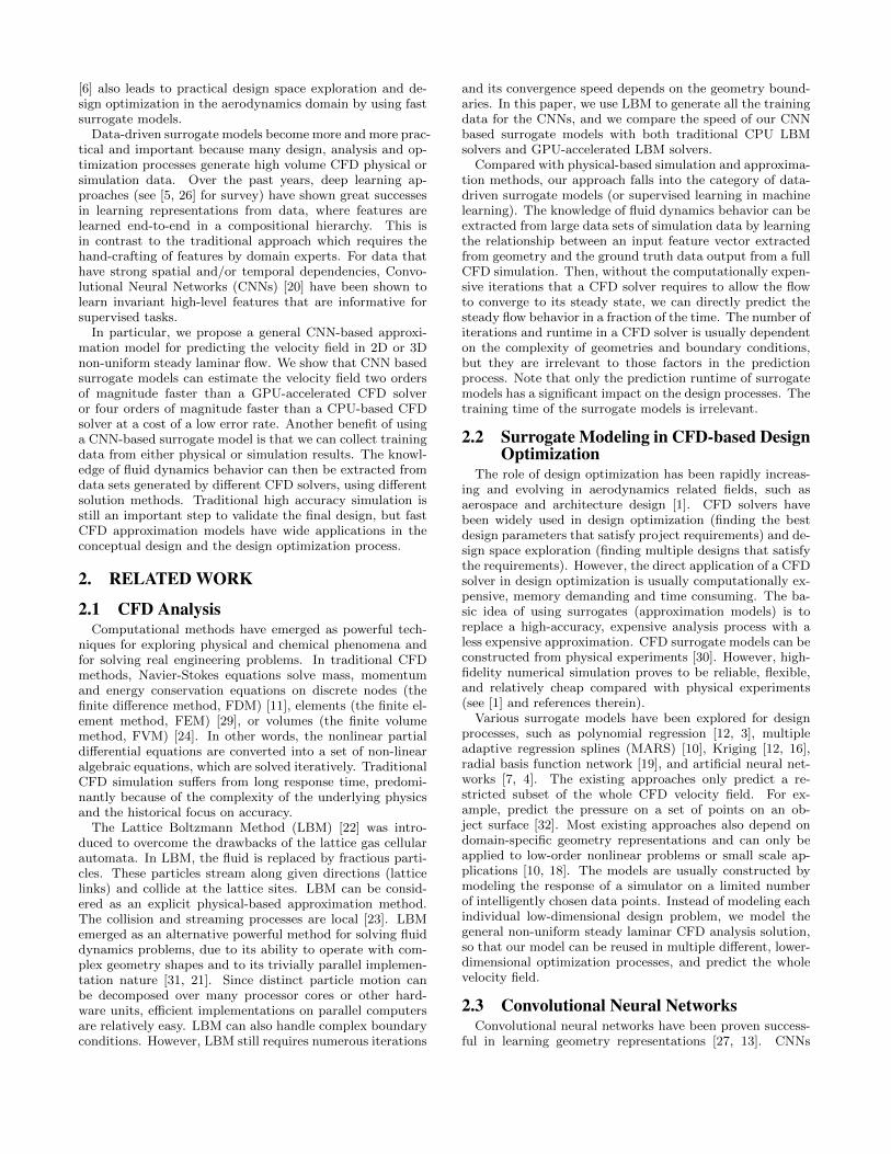
Figure 2: A discrete SDF representation of a cir-cle shape (zero level set) in a 23x14 Cartesian grid.The circle is shown in white. The magnitude of theSDF values on the Cartesian grid equals the minimaldistance to the circle.
A signed distance function D(i, j) associated to a level setfunction f(i, j) is defined by
D(i, j) = min(i′,j′)∈Z
∣∣(i, j)− (i′, j′)∣∣ sign(f(i, j)) (2)
D(i, j) is an oriented distance function and it measures thedistance of a given point (i, j) from the nearest boundary ofa closed geometrical shape Z, with the sign determined bywhether (i,j) is inside or outside the shape. Also, every pointoutside of the boundary has a value equal to its distance fromthe interface (see Figure 2 for a 2D SDF example).
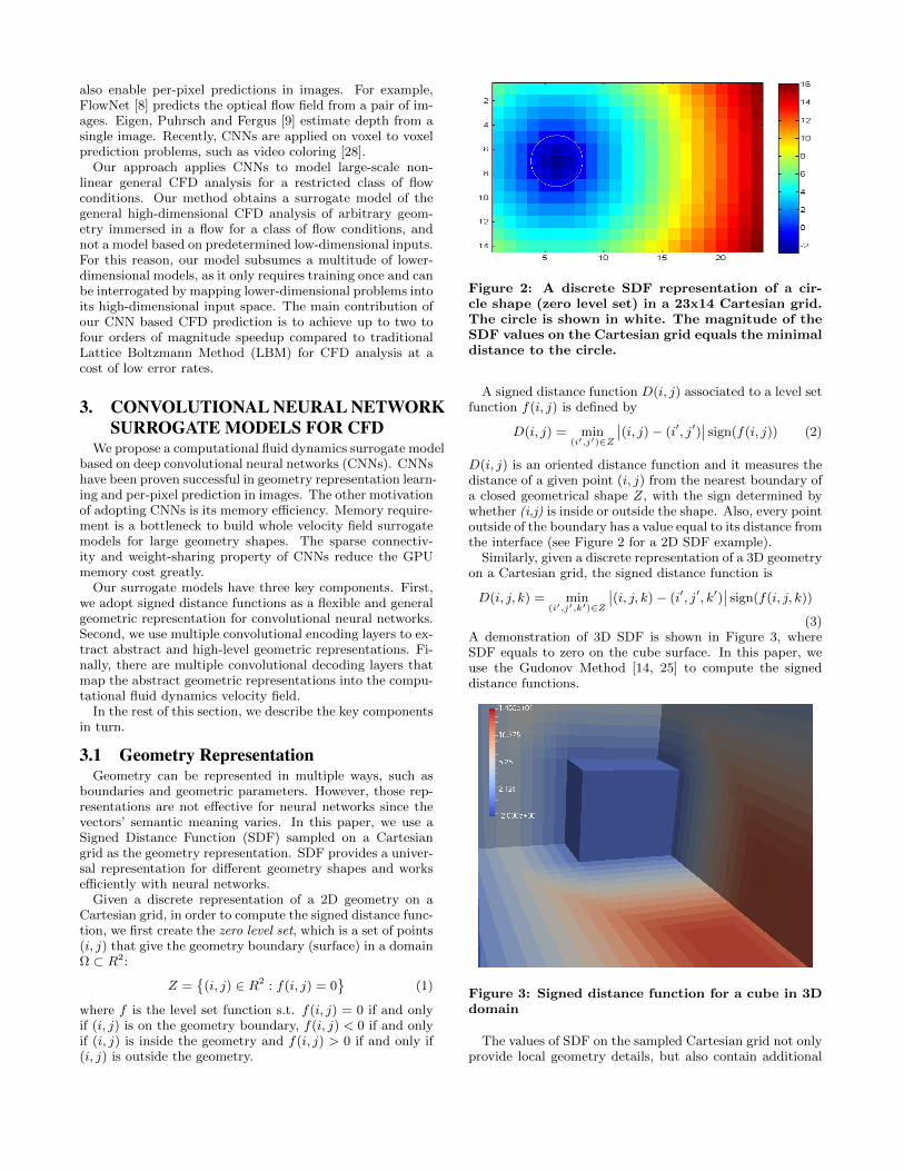
Similarly, given a discrete representation of a 3D geometryon a Cartesian grid, the signed distance function is
D(i, j, k) = min(i′,j′,k′)∈Z
∣∣(i, j, k)− (i′, j′, k′)∣∣ sign(f(i, j, k))
(3)A demonstration of 3D SDF is shown in Figure 3, whereSDF equals to zero on the cube surface. In this paper, weuse the Gudonov Method [14, 25] to compute the signeddistance functions.
Figure 3: Signed distance function for a cube in 3Ddomain
The values of SDF on the sampled Cartesian grid not onlyprovide local geometry details, but also contain additional
information of the global geometry structure. To validatethe efforts of computing SDF values in our experiments, wecompare the geometry representiveness of SDF and a simplebinary representation, where a grid value is 1 if and only ifit is within or on the boundary of geometry shapes. Suchbinary representations are easier to compute, but the valuesdo not provide any global structure information. We empir-ically show that SDF is more effective in representing thegeometry shapes for convolutional neural networks.
3.2 CFD SimulationIn this paper, we intend to leverage deep neural networks
as real-time surrogate models to substitute traditional time-consuming Lattice Boltzmann Method (LBM) CFD simula-tion [22]. LBM represents velocity fields as regular Cartesiangrids, or lattices, where each lattice cell represents the ve-locity field at that location. The LBM procedure updatesthe lattice iteratively, and usually the amount of requirediterations for the flow field to stabilize from a cold start islarge.
In LBM, geometry is represented by assigning an identifierto each lattice cell. This specific identifier defines whethera cell lies on the boundary or in the fluid domain. Fig-ure 4 illustrates this using an example of a 2D cylinder ina channel. In general, the LBM lattice cell resolution doesnot necessarily equal to the SDF resolution. In this work,we use the same geometry resolution in the LBM simulationand in the SDF representation. Thus, for a geometry withH ×W × D SDF representation, its CFD velocity field isalso H ×W × D. A 2D velocity field consists of two com-ponents x and y to represent the velocity components inx-direction and y-direction respectively. The velocity fieldfor 3D geometry has one additional z-component to repre-sent the velocity component in the z-direction.
Figure 4: 2D channel flow definition for LBM(1=fluid, 2=no-slip boundary, 3=velocity boundary,4=constant pressure boundary, 5=object boundary,0=internal)
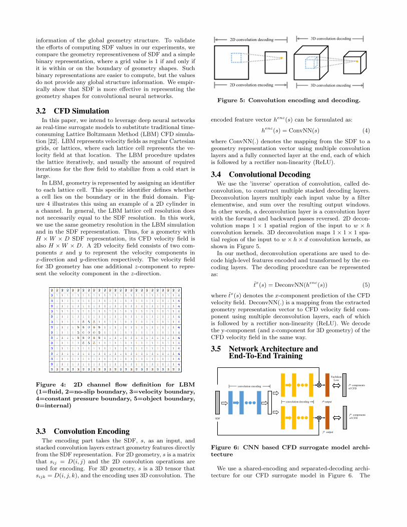
3.3 Convolution EncodingThe encoding part takes the SDF, s, as an input, and
stacked convolution layers extract geometry features directlyfrom the SDF representation. For 2D geometry, s is a matrixthat sij = D(i, j) and the 2D convolution operations areused for encoding. For 3D geometry, s is a 3D tensor thatsijk = D(i, j, k), and the encoding uses 3D convolution. The
2D convolution encoding
2D convolution decoding 3D convolution decoding
3D convolution encoding
Figure 5: Convolution encoding and decoding.
encoded feature vector henc(s) can be formulated as:
henc(s) = ConvNN(s) (4)
where ConvNN(.) denotes the mapping from the SDF to ageometry representation vector using multiple convolutionlayers and a fully connected layer at the end, each of whichis followed by a rectifier non-linearity (ReLU).
3.4 Convolutional DecodingWe use the ’inverse’ operation of convolution, called de-
convolution, to construct multiple stacked decoding layers.Deconvolution layers multiply each input value by a filterelementwise, and sum over the resulting output windows.In other words, a deconvolution layer is a convolution layerwith the forward and backward passes reversed. 2D decon-volution maps 1 × 1 spatial region of the input to w × hconvolution kernels. 3D deconvolution maps 1 × 1 × 1 spa-tial region of the input to w × h× d convolution kernels, asshown in Figure 5.
In our method, deconvolution operations are used to de-code high-level features encoded and transformed by the en-coding layers. The decoding procedure can be representedas:
tx(s) = DeconvNN(henc(s)) (5)
where tx(s) denotes the x-component prediction of the CFDvelocity field. DeconvNN(.) is a mapping from the extractedgeometry representation vector to CFD velocity field com-ponent using multiple deconvolution layers, each of whichis followed by a rectifier non-linearity (ReLU). We decodethe y-component (and z-component for 3D geometry) of theCFD velocity field in the same way.
3.5 Network Architecture andEnd-To-End Training
SDF
convolution encoding
convolution decoding ith output
jth output
ith components
of CFD
jth components
of CFD
Euclidean
Loss
Figure 6: CNN based CFD surrogate model archi-tecture
We use a shared-encoding and separated-decoding archi-tecture for our CFD surrogate model in Figure 6. The
shared-encoding saves computations compared to separated-encoding alternatives. Unlike encoding layers, decoding lay-ers are interfered by different velocity field components whena shared-decoding structure is used. In our shared-encodingand separated-decoding architecture, multiple convolutionallayers are used to extract an abstract geometry representa-tion, and the abstract geometry representation is used bymultiple decoding parts to generate the various componentsof the CFD velocity field. There are two decoding parts for2D geometry shapes and three for 3D geometry shapes. Analternative encoding structure is to use separated encodinglayers for each decoding part. In the experiment section, weshow that the prediction accuracy of the separated encodingstructure is similar to the shared encoding structure.
Further, we condition our CFD prediction based on theSDF to reduce errors. By definition, the velocity inside andon the boundary of geometry shapes is zero. Thus, the ve-locity field values change dramatically on the boundary ofgeometry shapes. SDF itself fully represents the boundaryinformation and our neural networks could condition theprediction by masking out the pixel or voxel inside or onthe boundary of the geometry. Such conditioned predic-tion eases the training and improve the prediction accuracy.The final prediction of our model is tx ⊗ 1s > 0, where1s > 0 is a binary mask and has the same size as s. Itselement is 1 if and only if the corresponding signed distancefunction value is greater than 0. ⊗ denotes element-wiseproduct.
We train our model to minimize the mean squared error:
L(θ) =1
N
N∑n=1
|tx(sn)⊗ 1sn > 0 − tx(sn)|2
+|ty(sn)⊗ 1sn > 0 − ty(sn)|2(6)
A similar loss function is defined for 3D geometry shapes:
L(θ) =1
N
N∑n=1
|tx(sn)⊗ 1sn > 0 − tx(sn)|2
+|ty(sn)⊗ 1sn > 0 − ty(sn)|2
+|tz(sn)⊗ 1sn > 0 − tz(sn)|2
(7)
4. EXPERIMENT SETUPIn the experiments, we evaluate our proposed method in
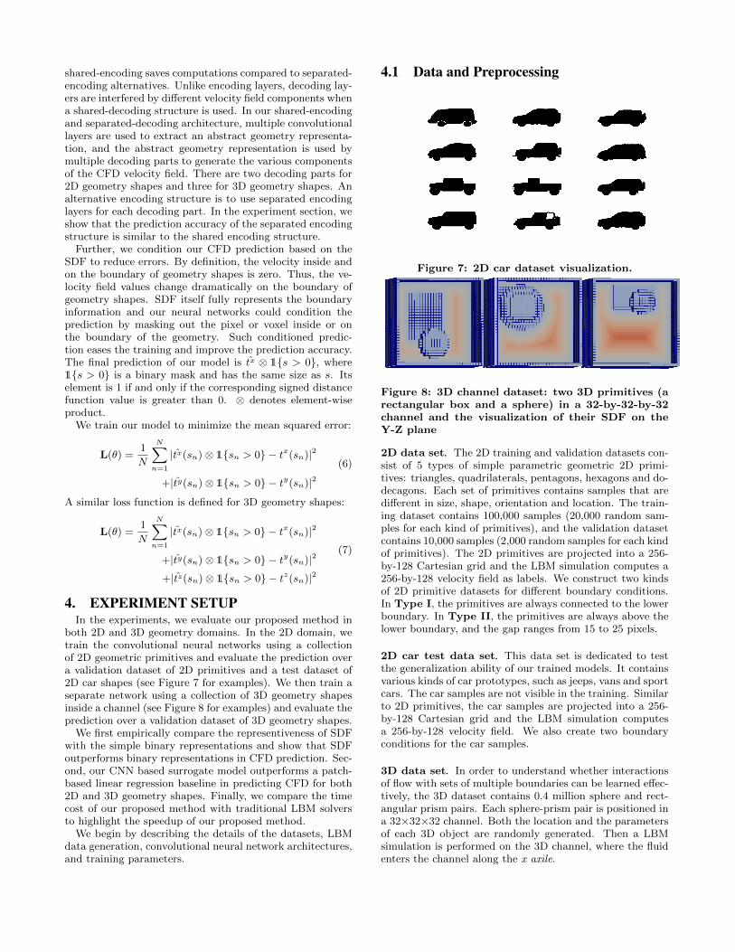
both 2D and 3D geometry domains. In the 2D domain, wetrain the convolutional neural networks using a collectionof 2D geometric primitives and evaluate the prediction overa validation dataset of 2D primitives and a test dataset of2D car shapes (see Figure 7 for examples). We then train aseparate network using a collection of 3D geometry shapesinside a channel (see Figure 8 for examples) and evaluate theprediction over a validation dataset of 3D geometry shapes.
We first empirically compare the representiveness of SDFwith the simple binary representations and show that SDFoutperforms binary representations in CFD prediction. Sec-ond, our CNN based surrogate model outperforms a patch-based linear regression baseline in predicting CFD for both2D and 3D geometry shapes. Finally, we compare the timecost of our proposed method with traditional LBM solversto highlight the speedup of our proposed method.
We begin by describing the details of the datasets, LBMdata generation, convolutional neural network architectures,and training parameters.
4.1 Data and Preprocessing
Figure 7: 2D car dataset visualization.
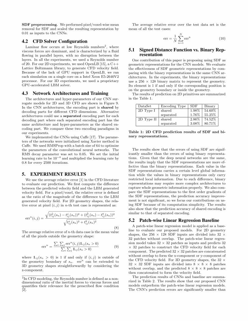
Figure 8: 3D channel dataset: two 3D primitives (arectangular box and a sphere) in a 32-by-32-by-32channel and the visualization of their SDF on theY-Z plane
2D data set. The 2D training and validation datasets con-sist of 5 types of simple parametric geometric 2D primi-tives: triangles, quadrilaterals, pentagons, hexagons and do-decagons. Each set of primitives contains samples that aredifferent in size, shape, orientation and location. The train-ing dataset contains 100,000 samples (20,000 random sam-ples for each kind of primitives), and the validation datasetcontains 10,000 samples (2,000 random samples for each kindof primitives). The 2D primitives are projected into a 256-by-128 Cartesian grid and the LBM simulation computes a256-by-128 velocity field as labels. We construct two kindsof 2D primitive datasets for different boundary conditions.In Type I, the primitives are always connected to the lowerboundary. In Type II, the primitives are always above thelower boundary, and the gap ranges from 15 to 25 pixels.
2D car test data set. This data set is dedicated to testthe generalization ability of our trained models. It containsvarious kinds of car prototypes, such as jeeps, vans and sportcars. The car samples are not visible in the training. Similarto 2D primitives, the car samples are projected into a 256-by-128 Cartesian grid and the LBM simulation computesa 256-by-128 velocity field. We also create two boundaryconditions for the car samples.
3D data set. In order to understand whether interactionsof flow with sets of multiple boundaries can be learned effec-tively, the 3D dataset contains 0.4 million sphere and rect-angular prism pairs. Each sphere-prism pair is positioned ina 32×32×32 channel. Both the location and the parametersof each 3D object are randomly generated. Then a LBMsimulation is performed on the 3D channel, where the fluidenters the channel along the x axile.
SDF preprocessing. We performed pixel/voxel-wise meanremoval for SDF and scaled the resulting representation by0.01 as inputs to the CNNs.
4.2 CFD Solver ConfigurationLaminar flow occurs at low Reynolds numbers2, where
viscous forces are dominant, and is characterized by a fluidflowing in parallel layers, with no disruption between thelayers. In all the experiments, we used a Reynolds numberof 20. For our 2D experiments, we used OpenLB [15], a C++Lattice Boltzmann library, to generate CFD velocity field.Because of the lack of GPU support in OpenLB, we raneach simulation on a single core on a Intel Xeon E5-2640V2processor. For our 3D experiments, we used a proprietaryGPU-accelerated LBM solver.
4.3 Network Architectures and TrainingThe architectures and hyper-parameters of our CNN sur-
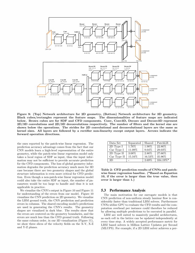
rogate models for 2D and 3D CFD are shown in Figure 9.In the CNN architectures, the encoding part is shared bydecoding parts for different CFD dimensions. Alternativearchitectures could use a separated encoding part for eachdecoding part where each separated encoding part has thesame architecture and hyper-parameters as the shared en-coding part. We compare these two encoding paradigms inour experiments.
We implemented the CNNs using Caffe [17]. The parame-ters of the networks were initialized using Xavier method inCaffe. We used RMSProp with a batch size of 64 to optimizethe parameters of the convolutional neural networks. TheRMS decay parameter was set to 0.05. We set the initiallearning rate to be 10−4 and multiplied the learning rate by0.8 for every 2500 iterations.
5. EXPERIMENT RESULTSWe use the average relative error [1] in the CFD literature
to evaluate our prediction. We first compute the differencebetween the predicted velocity field and the LBM generatedvelocity field. For a pixel/voxel, the relative error is definedas the ratio of the magnitude of the difference to the LBMgenerated velocity field. For 2D geometry shapes, the rela-tive error at pixel (i, j) in n-th test case is represented as:
errn(i, j) =
√(txij(sn)− txij(sn))2 + (tyij(sn)− tyij(sn))2√
txij(sn)2 + tyij(sn)2
(8)The average relative error of n-th data case is the mean valueof all the pixels outside the geometry shape:
errn =
∑i
∑j errn(i, j)1ij(sn > 0)∑i
∑j 1ij(sn > 0)
(9)
where 1ij(sn > 0) is 1 if and only if (i, j) is outside ofthe geometry boundary of sn. errn can be extended to3D geometry shapes straightforwardly by considering thez-component.
2In CFD modeling, the Reynolds number is defined as a non-dimensional ratio of the inertial forces to viscous forces andquantifies their relevance for the prescribed flow condition[2].
The average relative error over the test data set is themean of all the test cases:
err =1
N
N∑n=1
errn (10)
5.1 Signed Distance Function vs. Binary Rep-resentation
One contribution of this paper is proposing using SDF asgeometric representations for the CNN models. We evaluatethe effectiveness of SDF geometric representations by com-paring with the binary representations in the same CNN ar-chitectures. In the experiments, the binary representationsuse a 256 × 128 binary matrix to represent the geometry.Its element is 1 if and only if the corresponding position ison the geometry boundary or inside the geometry.
The results of prediction on 2D primitives are summarizedin the Table 1.
DataSet Encoding Type SDF Binary2D Type I shared 1.98% 54.60%
separated 1.76% 55.25%2D Type II shared 2.86% 74.52%
separated 3.08% 80.71%
Table 1: 2D CFD prediction results of SDF and bi-nary representations.
The results show that the errors of using SDF are signif-icantly smaller than the errors of using binary representa-tions. Given that the deep neural networks are the same,the results imply that the SDF representations are more ef-fective than the binary representations. Each value in theSDF representations carries a certain level global informa-tion while the values in binary representations only carryrestricted local information. Due to such difference, binaryrepresentations may require more complex architectures tocapture whole geometric information properly. We also com-pare the SDF representations to the first order gradients ofthe SDF representations, the prediction accuracy improve-ment is not significant, so we focus our contributions on us-ing SDF because of its computation simplicity. The resultsalso show that the prediction accuracy of shared encoding issimilar to that of separated encoding.
5.2 Patch-wise Linear Regression BaselineA patch-wise linear regression model is applied as a base-
line to evaluate our proposed models. For 2D geometryshapes, the 256 × 128 SDF inputs are divided into 32 ×32 patches without overlap. The patch-wise linear regres-sion model takes 32 × 32 patches as inputs and predicts 32× 32 patches to construct the CFD velocity field for eachcomponent. The predicted 32× 32 patches are concatenatedwithout overlap to form the x-component or y-component ofthe CFD velocity field. For 3D geometry shapes, the 32 ×32 × 32 SDF inputs are divided into 8 × 8 × 8 patcheswithout overlap, and the predicted 8 × 8 × 8 patches arethen concatenated to form the velocity field.
The prediction results of CNNs and baseline are summa-rized in Table 2. The results show that our proposed CNNmodels outperform the patch-wise linear regression models.The CNN’s prediction errors are significantly smaller than
256×128
16×16×128
Conv
128, 16×8
Conv
512, 4×4
x-component
of CFD
1024
FullCon
Deconv
512, 8×8
4×4×512
8×8×512
Deconv
256, 8×4
64×32×256 128×64×32
Deconv
32, 2×2
Deconv
1, 2×2
256×128
8×8×512 64×32×256 128×64×32
256×128
y-component
of CFD
256×128
256×128
32×32×32
15×15×15×32
Conv3D
32, 4×4×4stride 2
x-component
of CFD
512
FullCon
Deconv3D
128, 3×3×3
stride 1
7×7×7×64
Conv3D
64, 3×3×3stride 2
Conv3D
128, 3×3×3stride 2
3×3×3×128
Deconv3D
64, 3×3×3
stride 2
3×3×3×128
Deconv3D
32, 3×3×3
stride 2
7×7×7×64 15×15×15×32
Deconv3D
1, 4×4×4
stride 2
32×32×32
y-component
of CFD
3×3×3×128 7×7×7×64 15×15×15×32 32×32×32
z-component
of CFD
3×3×3×128 7×7×7×64 15×15×15×32 32×32×3232×32×32
32×32×32
32×32×32
Figure 9: (Top) Network architecture for 2D geometry, (Bottom) Network architecture for 3D geometry.Black cubes/rectangles represent the feature maps. The dimensionalities of feature maps are indicatedbelow. Brown cubes are for SDF and CFD components. Conv, Conv3D, Deconv and Deconv3D represent2D/3D convolutions and 2D/3D deconvolutions respectively. The number of filters and the kernel size areshown below the operations. The strides for 2D convolutional and deconvolutional layers are the same askernel sizes. All layers are followed by a rectifier non-linearity except output layers. Arrows indicate theforward operation directions.
the ones reported by the patch-wise linear regression. Theprediction accuracy advantage comes from the fact that ourCNN models learn a high-level representation of the entiregeometry, while the patch-wise linear regression model onlytakes a local region of SDF as input, thus the input infor-mation may not be sufficient to provide accurate predictionfor the CFD components. The loss of global geometry infor-mation degrades the prediction accuracy much more for 3Dcase because there are two geometry shapes and the globalstructure information is even more critical for CFD predic-tion. Even though a non-patch-wise linear regression modelcould also take the entire SDF as input, the number of pa-rameters would be too large to handle and thus it is notapplicable in practice.
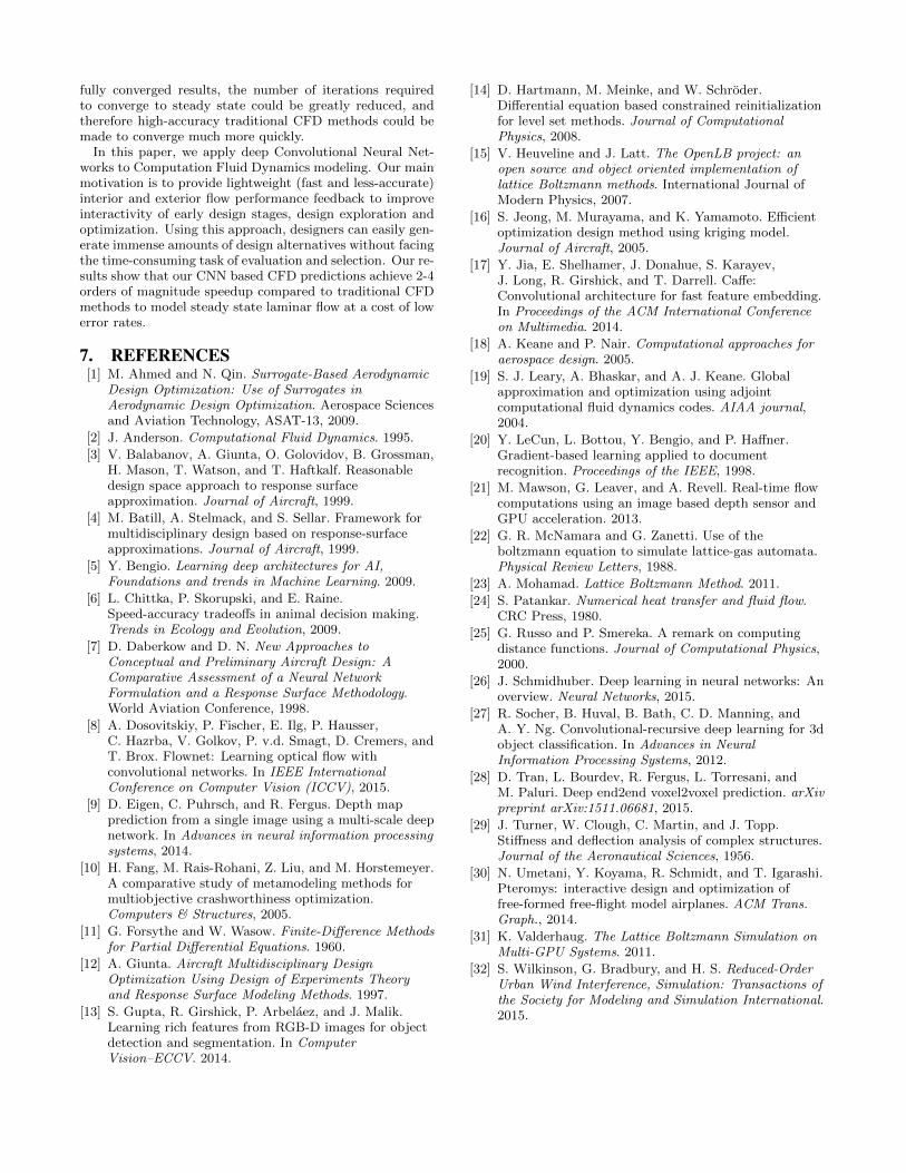
We visualize the CNN’s output in Figure 10 and Figure 11for understanding of the errors from our model. Figure 10visualizes the CNN prediction on 2D geometry. We visualizethe LBM ground truth, the CNN prediction and predictionerrors in columns. The shared encoding model’s predictionsare used in generating the CNN’s results. The geometryshapes are visualized in dark blue. The results show thatthe errors are centered on the geometry boundaries, and theerrors are much less than the CFD ground truth. Followingthe same column order, in our 3D visualization (Figure 11),we show three slices of the velocity fields on the X-Y, X-Zand Y-Z planes.
Data Set Separated Shared PatchLR2D Type I 1.76% 1.98% 22.86%Car Type I 11.09% 9.04% 29.03%2D Type II 3.08% 2.86% 27.66%Car Type II 15.34% 16.53% 35.96%3D - 2.69% 334.19%*
Table 2: CFD prediction results of CNNs and patch-wise linear regression baseline. (*Based on Equation10, if the error is larger than the true value, thenerror is larger than 1.)
5.3 Performance AnalysisThe main motivation for our surrogate models is that
CNN prediction of non-uniform steady laminar flow is con-siderably faster than traditional LBM solvers. FurthermoreCNNs utilize GPU to evaluate the CFD results and the com-putation overhead per instance could therefore be reducedby allowing multiple predictions to be executed in parallel.
LBM are well suited to massively parallel architectures,as each cell in the lattice can be updated independently atevery time step. A widely accepted performance metric forLBM based solvers is Million Lattice Updates per Second(MLUPS). For example, if a 2D LBM solver achieves a per-
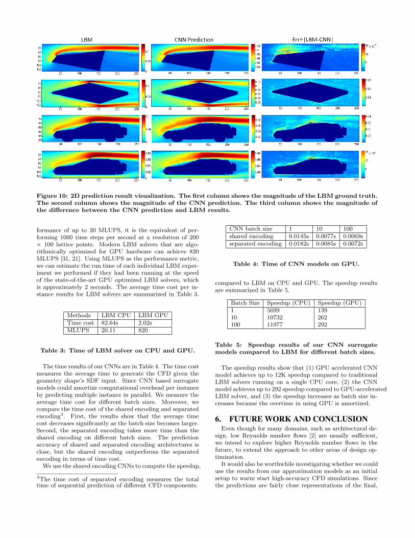
Figure 10: 2D prediction result visualization. The first column shows the magnitude of the LBM ground truth.The second column shows the magnitude of the CNN prediction. The third column shows the magnitude ofthe difference between the CNN prediction and LBM results.
formance of up to 20 MLUPS, it is the equivalent of per-forming 1000 time steps per second at a resolution of 200× 100 lattice points. Modern LBM solvers that are algo-rithmically optimized for GPU hardware can achieve 820MLUPS [31, 21]. Using MLUPS as the performance metric,we can estimate the run time of each individual LBM exper-iment we performed if they had been running at the speedof the state-of-the-art GPU optimized LBM solvers, whichis approximately 2 seconds. The average time cost per in-stance results for LBM solvers are summarized in Table 3.
Methods LBM CPU LBM GPUTime cost 82.64s 2.02sMLUPS 20.11 820
Table 3: Time of LBM solver on CPU and GPU.
The time results of our CNNs are in Table 4. The time costmeasures the average time to generate the CFD given thegeometry shape’s SDF input. Since CNN based surrogatemodels could amortize computational overhead per instanceby predicting multiple instance in parallel. We measure theaverage time cost for different batch sizes. Moreover, wecompare the time cost of the shared encoding and separatedencoding3. First, the results show that the average timecost decreases significantly as the batch size becomes larger.Second, the separated encoding takes more time than theshared encoding on different batch sizes. The predictionaccuracy of shared and separated encoding architectures isclose, but the shared encoding outperforms the separatedencoding in terms of time cost.
We use the shared encoding CNNs to compute the speedup,
3The time cost of separated encoding measures the totaltime of sequential prediction of different CFD components.
CNN batch size 1 10 100shared encoding 0.0145s 0.0077s 0.0069sseparated encoding 0.0182s 0.0085s 0.0072s
Table 4: Time of CNN models on GPU.
compared to LBM on CPU and GPU. The speedup resultsare summarized in Table 5.
Batch Size Speedup (CPU) Speedup (GPU)1 5699 13910 10732 262100 11977 292
Table 5: Speedup results of our CNN surrogatemodels compared to LBM for different batch sizes.
The speedup results show that (1) GPU accelerated CNNmodel achieves up to 12K speedup compared to traditionalLBM solvers running on a single CPU core, (2) the CNNmodel achieves up to 292 speedup compared to GPU-acceleratedLBM solver, and (3) the speedup increases as batch size in-creases because the overtime in using GPU is amortized.
6. FUTURE WORK AND CONCLUSIONEven though for many domains, such as architectural de-
sign, low Reynolds number flows [2] are usually sufficient,we intend to explore higher Reynolds number flows in thefuture, to extend the approach to other areas of design op-timization.
It would also be worthwhile investigating whether we coulduse the results from our approximation models as an initialsetup to warm start high-accuracy CFD simulations. Sincethe predictions are fairly close representations of the final,
fully converged results, the number of iterations requiredto converge to steady state could be greatly reduced, andtherefore high-accuracy traditional CFD methods could bemade to converge much more quickly.
In this paper, we apply deep Convolutional Neural Net-works to Computation Fluid Dynamics modeling. Our mainmotivation is to provide lightweight (fast and less-accurate)interior and exterior flow performance feedback to improveinteractivity of early design stages, design exploration andoptimization. Using this approach, designers can easily gen-erate immense amounts of design alternatives without facingthe time-consuming task of evaluation and selection. Our re-sults show that our CNN based CFD predictions achieve 2-4orders of magnitude speedup compared to traditional CFDmethods to model steady state laminar flow at a cost of lowerror rates.
7. REFERENCES[1] M. Ahmed and N. Qin. Surrogate-Based Aerodynamic
Design Optimization: Use of Surrogates inAerodynamic Design Optimization. Aerospace Sciencesand Aviation Technology, ASAT-13, 2009.
[2] J. Anderson. Computational Fluid Dynamics. 1995.
[3] V. Balabanov, A. Giunta, O. Golovidov, B. Grossman,H. Mason, T. Watson, and T. Haftkalf. Reasonabledesign space approach to response surfaceapproximation. Journal of Aircraft, 1999.
[4] M. Batill, A. Stelmack, and S. Sellar. Framework formultidisciplinary design based on response-surfaceapproximations. Journal of Aircraft, 1999.
[5] Y. Bengio. Learning deep architectures for AI,Foundations and trends in Machine Learning. 2009.
[6] L. Chittka, P. Skorupski, and E. Raine.Speed-accuracy tradeoffs in animal decision making.Trends in Ecology and Evolution, 2009.
[7] D. Daberkow and D. N. New Approaches toConceptual and Preliminary Aircraft Design: AComparative Assessment of a Neural NetworkFormulation and a Response Surface Methodology.World Aviation Conference, 1998.
[8] A. Dosovitskiy, P. Fischer, E. Ilg, P. Hausser,C. Hazrba, V. Golkov, P. v.d. Smagt, D. Cremers, andT. Brox. Flownet: Learning optical flow withconvolutional networks. In IEEE InternationalConference on Computer Vision (ICCV), 2015.
[9] D. Eigen, C. Puhrsch, and R. Fergus. Depth mapprediction from a single image using a multi-scale deepnetwork. In Advances in neural information processingsystems, 2014.
[10] H. Fang, M. Rais-Rohani, Z. Liu, and M. Horstemeyer.A comparative study of metamodeling methods formultiobjective crashworthiness optimization.Computers & Structures, 2005.
[11] G. Forsythe and W. Wasow. Finite-Difference Methodsfor Partial Differential Equations. 1960.
[12] A. Giunta. Aircraft Multidisciplinary DesignOptimization Using Design of Experiments Theoryand Response Surface Modeling Methods. 1997.
[13] S. Gupta, R. Girshick, P. Arbelaez, and J. Malik.Learning rich features from RGB-D images for objectdetection and segmentation. In ComputerVision–ECCV. 2014.
[14] D. Hartmann, M. Meinke, and W. Schroder.Differential equation based constrained reinitializationfor level set methods. Journal of ComputationalPhysics, 2008.
[15] V. Heuveline and J. Latt. The OpenLB project: anopen source and object oriented implementation oflattice Boltzmann methods. International Journal ofModern Physics, 2007.
[16] S. Jeong, M. Murayama, and K. Yamamoto. Efficientoptimization design method using kriging model.Journal of Aircraft, 2005.
[17] Y. Jia, E. Shelhamer, J. Donahue, S. Karayev,J. Long, R. Girshick, and T. Darrell. Caffe:Convolutional architecture for fast feature embedding.In Proceedings of the ACM International Conferenceon Multimedia. 2014.
[18] A. Keane and P. Nair. Computational approaches foraerospace design. 2005.
[19] S. J. Leary, A. Bhaskar, and A. J. Keane. Globalapproximation and optimization using adjointcomputational fluid dynamics codes. AIAA journal,2004.
[20] Y. LeCun, L. Bottou, Y. Bengio, and P. Haffner.Gradient-based learning applied to documentrecognition. Proceedings of the IEEE, 1998.
[21] M. Mawson, G. Leaver, and A. Revell. Real-time flowcomputations using an image based depth sensor andGPU acceleration. 2013.
[22] G. R. McNamara and G. Zanetti. Use of theboltzmann equation to simulate lattice-gas automata.Physical Review Letters, 1988.
[23] A. Mohamad. Lattice Boltzmann Method. 2011.
[24] S. Patankar. Numerical heat transfer and fluid flow.CRC Press, 1980.
[25] G. Russo and P. Smereka. A remark on computingdistance functions. Journal of Computational Physics,2000.
[26] J. Schmidhuber. Deep learning in neural networks: Anoverview. Neural Networks, 2015.
[27] R. Socher, B. Huval, B. Bath, C. D. Manning, andA. Y. Ng. Convolutional-recursive deep learning for 3dobject classification. In Advances in NeuralInformation Processing Systems, 2012.
[28] D. Tran, L. Bourdev, R. Fergus, L. Torresani, andM. Paluri. Deep end2end voxel2voxel prediction. arXivpreprint arXiv:1511.06681, 2015.
[29] J. Turner, W. Clough, C. Martin, and J. Topp.Stiffness and deflection analysis of complex structures.Journal of the Aeronautical Sciences, 1956.
[30] N. Umetani, Y. Koyama, R. Schmidt, and T. Igarashi.Pteromys: interactive design and optimization offree-formed free-flight model airplanes. ACM Trans.Graph., 2014.
[31] K. Valderhaug. The Lattice Boltzmann Simulation onMulti-GPU Systems. 2011.
[32] S. Wilkinson, G. Bradbury, and H. S. Reduced-OrderUrban Wind Interference, Simulation: Transactions ofthe Society for Modeling and Simulation International.2015.
Figure 11: 3D prediction visualization. The first column shows the magnitude of the LBM ground truth.The second column shows the magnitude of the CNN prediction. The third column shows the magnitude ofthe difference between the CNN prediction and LBM results.