verification of quantitative precipitation ... - cawcr.gov.au · verification of quantitative...
TRANSCRIPT
VERIFICATION OF QUANTITATIVE PRECIPITATION FORECASTS USING
BADDELEY’S DELTA METRIC
Thomas C.M. Lee, Eric Gilleland, Barb Brown and Randy Bullock
National Center for Atmospheric Research
Research Applications Division
1
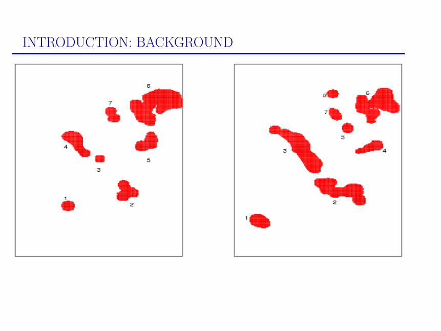
INTRODUCTION: BACKGROUND
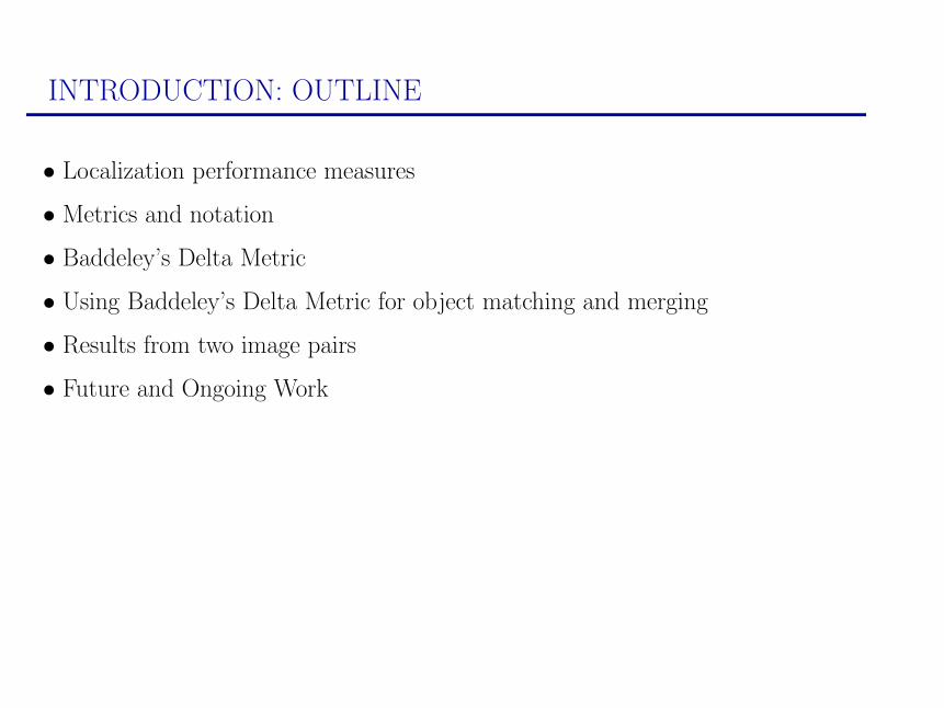
INTRODUCTION: OUTLINE
• Localization performance measures
• Metrics and notation
• Baddeley’s Delta Metric
• Using Baddeley’s Delta Metric for object matching and merging
• Results from two image pairs
• Future and Ongoing Work
3
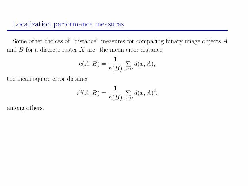
Localization performance measures
Some other choices of “distance” measures for comparing binary image objects A
and B for a discrete raster X are: the mean error distance,
e(A, B) =1
n(B)
∑x∈B
d(x, A),
the mean square error distance
e2(A, B) =1
n(B)
∑x∈B
d(x, A)2,
among others.
4
Localization performance measures: some problems
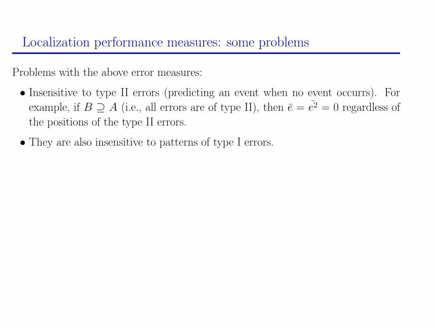
Problems with the above error measures:
• Insensitive to type II errors (predicting an event when no event occurrs). For
example, if B ⊇ A (i.e., all errors are of type II), then e = e2 = 0 regardless of
the positions of the type II errors.
• They are also insensitive to patterns of type I errors.
5
Metrics and notation
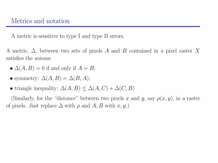
A metric is sensitive to type I and type II errors.
A metric, ∆, between two sets of pixels A and B contained in a pixel raster X
satisfies the axioms
• ∆(A, B) = 0 if and only if A = B;
• symmetry: ∆(A, B) = ∆(B, A);
• triangle inequality: ∆(A, B) ≤ ∆(A, C) + ∆(C, B)
(Similarly, for the “distance” between two pixels x and y, say ρ(x, y), in a raster
of pixels. Just replace ∆ with ρ and A, B with x, y.)
6
Metrics and notation
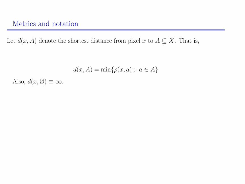
Let d(x, A) denote the shortest distance from pixel x to A ⊆ X . That is,
d(x, A) = min{ρ(x, a) : a ∈ A}
Also, d(x, Ø) ≡ ∞.
7
Metrics and notation
d(·, A) can be computed rapidly by the distance transform algorithm. See, for ex-
ample:
Borgefors, G. Distance transformations in digital images. Computer Vision, Graph-
ics and Image Processing, 34:344–371, 1986.
Rosenfeld and Pfalz, J.L. Sequential operations in digital picture processing. Jour-
nal of the Association for Computing Machinery, 13:471, 1966.
Rosenfeld and Pfalz, J.L. Distance functions on digital pictures. Pattern Recogni-
tion, 1:33–61, 1968.
8
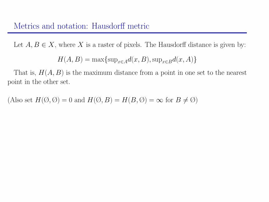
Metrics and notation: Hausdorff metric
Let A, B ∈ X , where X is a raster of pixels. The Hausdorff distance is given by:
H(A, B) = max{supx∈Ad(x, B), supx∈Bd(x, A)}
That is, H(A, B) is the maximum distance from a point in one set to the nearest
point in the other set.
(Also set H(Ø, Ø) = 0 and H(Ø, B) = H(B, Ø) = ∞ for B 6= Ø)
9
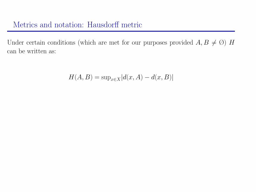
Metrics and notation: Hausdorff metric
Under certain conditions (which are met for our purposes provided A, B 6= Ø) H
can be written as:
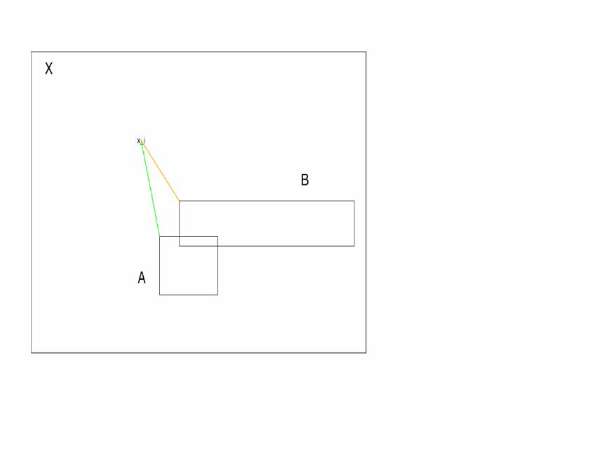
H(A, B) = supx∈X|d(x, A)− d(x, B)|
10
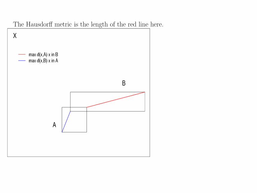
The Hausdorff metric is the length of the red line here.
11
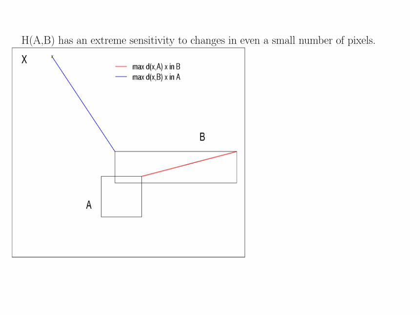
H(A,B) has an extreme sensitivity to changes in even a small number of pixels.
12
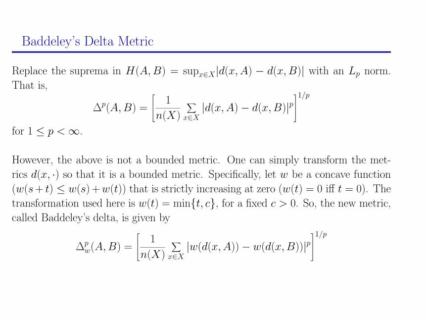
Baddeley’s Delta Metric
Replace the suprema in H(A, B) = supx∈X|d(x, A) − d(x, B)| with an Lp norm.
That is,
∆p(A, B) =
1
n(X)
∑x∈X
|d(x, A)− d(x, B)|p1/p
for 1 ≤ p < ∞.
However, the above is not a bounded metric. One can simply transform the met-
rics d(x, ·) so that it is a bounded metric. Specifically, let w be a concave function
(w(s + t) ≤ w(s) + w(t)) that is strictly increasing at zero (w(t) = 0 iff t = 0). The
transformation used here is w(t) = min{t, c}, for a fixed c > 0. So, the new metric,
called Baddeley’s delta, is given by
∆pw(A, B) =
1
n(X)
∑x∈X
|w(d(x, A))− w(d(x, B))|p1/p
13
14
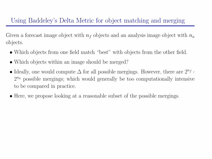
Using Baddeley’s Delta Metric for object matching and merging
Given a forecast image object with nf objects and an analysis image object with na
objects.
• Which objects from one field match “best” with objects from the other field.
• Which objects within an image should be merged?
• Ideally, one would compute ∆ for all possible mergings. However, there are 2nf ·2na possible mergings; which would generally be too computationally intensive
to be compared in practice.
• Here, we propose looking at a reasonable subset of the possible mergings.
15
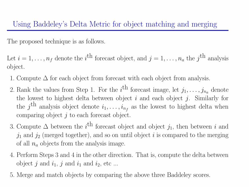
Using Baddeley’s Delta Metric for object matching and merging
The proposed technique is as follows.
Let i = 1, . . . , nf denote the ith forecast object, and j = 1, . . . , na the jth analysis
object.
1. Compute ∆ for each object from forecast with each object from analysis.
2. Rank the values from Step 1. For the ith forecast image, let j1, . . . , jna denote
the lowest to highest delta between object i and each object j. Similarly for
the jth analysis object denote i1, . . . , infas the lowest to highest delta when
comparing object j to each forecast object.
3. Compute ∆ between the ith forecast object and object j1, then between i and
j1 and j2 (merged together), and so on until object i is compared to the merging
of all na objects from the analysis image.
4. Perform Steps 3 and 4 in the other direction. That is, compute the delta between
object j and i1, j and i1 and i2, etc ...
5. Merge and match objects by comparing the above three Baddeley scores.
16
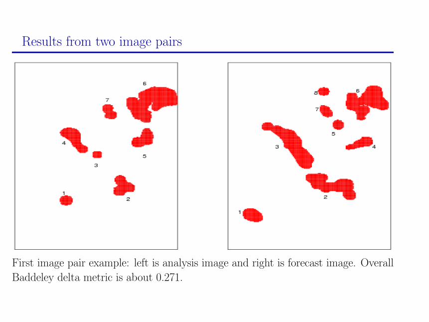
Results from two image pairs
First image pair example: left is analysis image and right is forecast image. Overall
Baddeley delta metric is about 0.271.
17
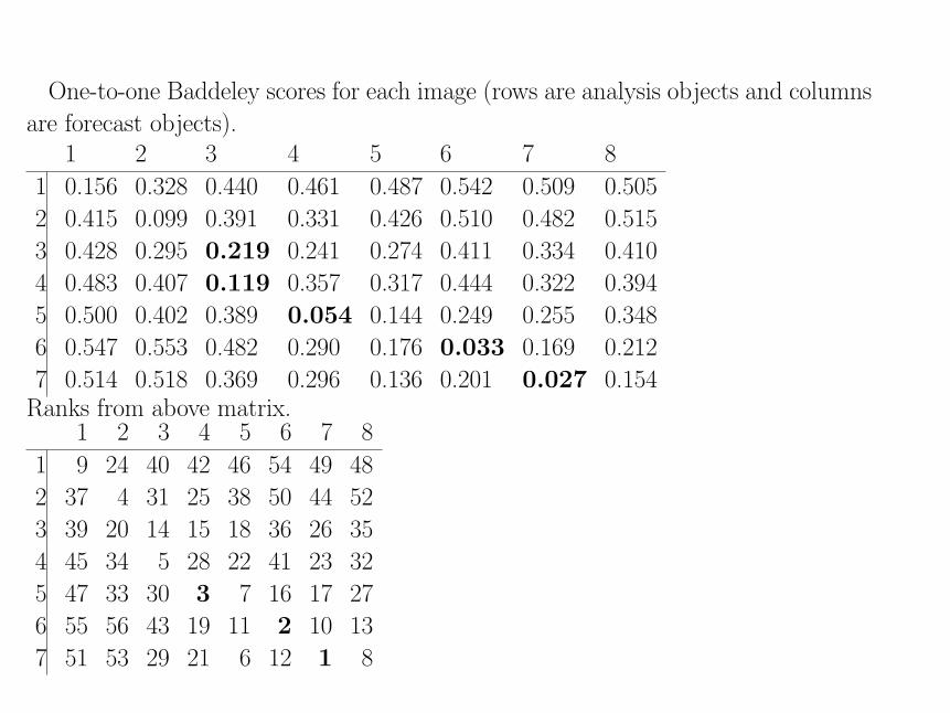
One-to-one Baddeley scores for each image (rows are analysis objects and columns
are forecast objects).1 2 3 4 5 6 7 8
1 0.156 0.328 0.440 0.461 0.487 0.542 0.509 0.505
2 0.415 0.099 0.391 0.331 0.426 0.510 0.482 0.515
3 0.428 0.295 0.219 0.241 0.274 0.411 0.334 0.410
4 0.483 0.407 0.119 0.357 0.317 0.444 0.322 0.394
5 0.500 0.402 0.389 0.054 0.144 0.249 0.255 0.348
6 0.547 0.553 0.482 0.290 0.176 0.033 0.169 0.212
7 0.514 0.518 0.369 0.296 0.136 0.201 0.027 0.154Ranks from above matrix.
1 2 3 4 5 6 7 8
1 9 24 40 42 46 54 49 48
2 37 4 31 25 38 50 44 52
3 39 20 14 15 18 36 26 35
4 45 34 5 28 22 41 23 32
5 47 33 30 3 7 16 17 27
6 55 56 43 19 11 2 10 13
7 51 53 29 21 6 12 1 8
18
19
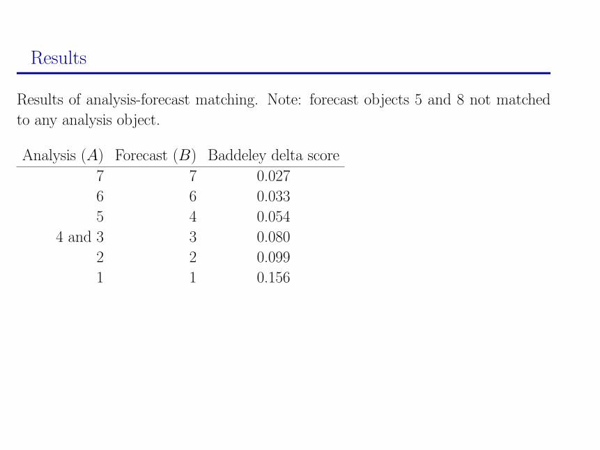
Results
Results of analysis-forecast matching. Note: forecast objects 5 and 8 not matched
to any analysis object.
Analysis (A) Forecast (B) Baddeley delta score
7 7 0.027
6 6 0.033
5 4 0.054
4 and 3 3 0.080
2 2 0.099
1 1 0.156
20

21
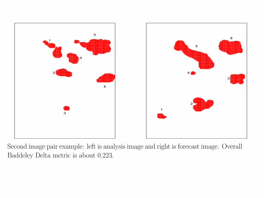
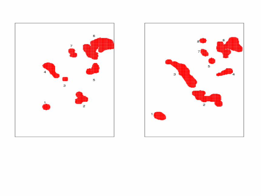
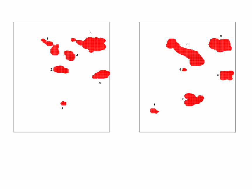
Second image pair example: left is analysis image and right is forecast image. Overall
Baddeley Delta metric is about 0.223.
22
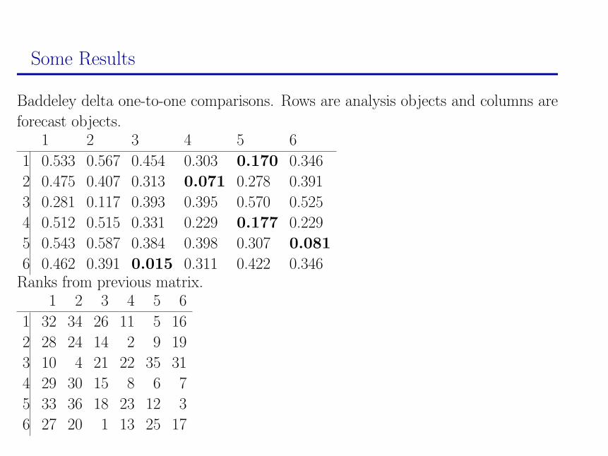
Some Results
Baddeley delta one-to-one comparisons. Rows are analysis objects and columns are
forecast objects.1 2 3 4 5 6
1 0.533 0.567 0.454 0.303 0.170 0.346
2 0.475 0.407 0.313 0.071 0.278 0.391
3 0.281 0.117 0.393 0.395 0.570 0.525
4 0.512 0.515 0.331 0.229 0.177 0.229
5 0.543 0.587 0.384 0.398 0.307 0.081
6 0.462 0.391 0.015 0.311 0.422 0.346Ranks from previous matrix.
1 2 3 4 5 6
1 32 34 26 11 5 16
2 28 24 14 2 9 19
3 10 4 21 22 35 31
4 29 30 15 8 6 7
5 33 36 18 23 12 3
6 27 20 1 13 25 17
23
24
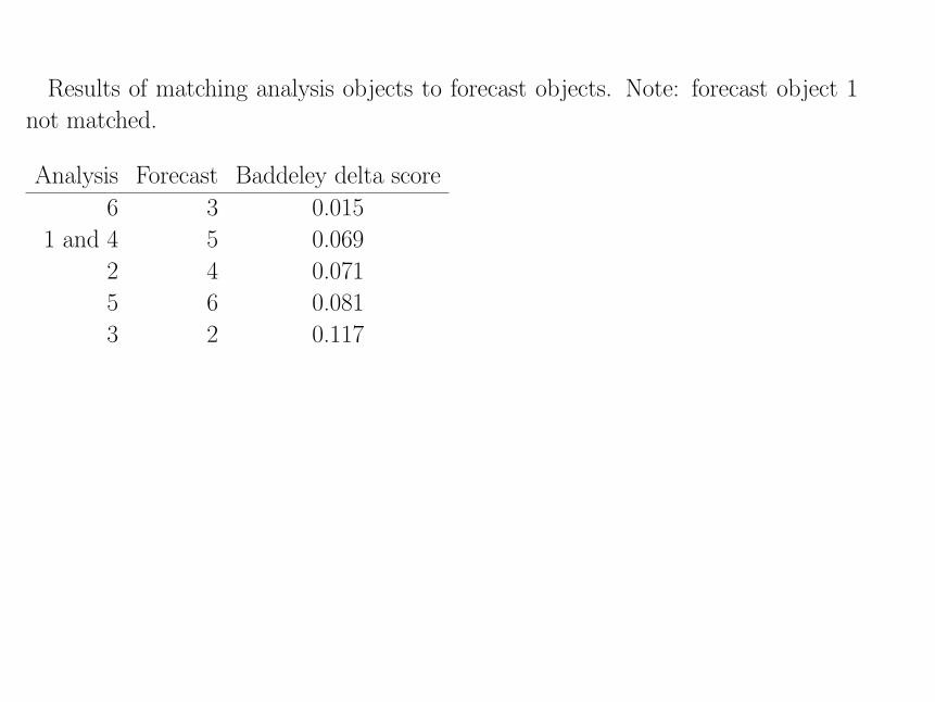
Results of matching analysis objects to forecast objects. Note: forecast object 1
not matched.
Analysis Forecast Baddeley delta score
6 3 0.015
1 and 4 5 0.069
2 4 0.071
5 6 0.081
3 2 0.117
25

26
Future and Ongoing Work
• How to combine information from “best” matches/merges to give a summary
score based on the Baddeley delta.
• What constitutes a “good” Baddeley delta score (have a human expert judge
several cases?).
• How to incorporate into overall verification scheme.
• Characteristics/distributions of ∆’s.
• How to compare with Fuzzy Logic analysis of Bullock et al.
27
References
Baddeley, A.J., 1992: Errors in binary images and an Lp version of the Hausdorff
metric, Nieuw Archief voor Wiskunde, 10: 157–183.
Baddeley, A.J., 1992: An error metric for binary images, In W. Forstner and S.
Ruwiedel (ed.) Robust Computer Vision Algorithms, Proceedings, Interna-
tional Workshop on Robust Computer Vision, Bonn. Karlsruhe: Wichmann,
59–78.See: http://www.maths.uwa.edu.au/~adrian/metrics.html
28