climate change science and victoria - cawcr.gov.au · climate change science and victoria i climate...
TRANSCRIPT

Bureau Research Report – 014
Climate change science and Victoria
Bertrand Timbal, Marie Ekström, Sonya Fiddes, Michael Grose, Dewi Kirono, Eun-Pa Lim, Chris Lucas and Louise Wilson
May 2016


CLIMATE CHANGE SCIENCE AND VICTORIA
i
Climate change science and Victoria
Bertrand Timbal, Marie Ekström, Sonya Fiddes, Michael Grose, Dewi Kirono, Eun-Pa Lim, Chris Lucas and Louise Wilson
Bureau Research Report No. 014
May 2016
National Library of Australia Cataloguing-in-Publication entry
Creator: Timbal, Bertrand, author
Title: Climate change science and Victoria / Bertrand Timbal, Marie Ekström, Sonya Fiddes, Michael
Grose, Dewi Kirono, Eun-Pa Lim, Chris Lucas and Louise Wilson
ISBN: 9780642706744 (ebook)
Series: Bureau research reports; BRR-014.
Other Creators/Contributors:
Marie Ekström, author.
Sonya Fiddes, author.
Michael Grose, author.
Dewi Kirono, author.
Eun-Pa Lim, author.
Chris Lucas, author.
Louise Wilson, author.
Australia. Bureau of Meteorology, issuing body.

CLIMATE CHANGE SCIENCE AND VICTORIA
ii
Enquiries should be addressed to:
Contact Name: Bertrand Timbal
Bureau of Meteorology
GPO Box 1289, Melbourne
Victoria 3001, Australia
Contact Email: [email protected]
Copyright and Disclaimer
© 2016 Bureau of Meteorology. To the extent permitted by law, all rights are reserved and no part of
this publication covered by copyright may be reproduced or copied in any form or by any means
except with the written permission of the Bureau of Meteorology.
The Bureau of Meteorology advise that the information contained in this publication comprises
general statements based on scientific research. The reader is advised and needs to be aware that such
information may be incomplete or unable to be used in any specific situation. No reliance or actions
must therefore be made on that information without seeking prior expert professional, scientific and
technical advice. To the extent permitted by law and the Bureau of Meteorology (including each of its
employees and consultants) excludes all liability to any person for any consequences, including but
not limited to all losses, damages, costs, expenses and any other compensation, arising directly or
indirectly from using this publication (in part or in whole) and any information or material contained
in it.

CLIMATE CHANGE SCIENCE AND VICTORIA
iii
Acknowledgments
Additional contributor acknowledgements: Gnanathikkam Amirthanathan, Janice Bathols, Tim
Bedin, Jonas Bhend, John Clarke, Tim Erwin, Alex Evans, Harry Hendon, Kathleen McInnes,
Freddie Mpelasoka, Aurel Moise, Hanh Nguyen, Nick Potter, Surendra Rauniyar, Robert
Smalley, Yang Wang, Ian Watterson, Leanne Web.
Peer review: Rae Moran (independent expert), Mike Manton (independent expert), Blair Trewin
(Bureau of Meteorology), Aurel Moise (Bureau of Meteorology), John Clarke (CSIRO) and
Penny Whetton (CSIRO).
We acknowledge the project funding provided through the Victorian Climate Initiative by the
Victorian Department of the Environment, Land, Water and Planning (DELWP), and the BOM
and CSIRO.
We acknowledge the Regional Natural Resource Management planning for Climate Change
Project which delivered the national climate change projections and the Department of the
Environment from the Australian Government which supported this project.
We acknowledge the World Climate Research Programme’s Working Group on Coupled
Modelling, which is responsible for CMIP, and we thank the climate modelling groups (listed in
Appendix 3) for producing and making available their model output. For CMIP the U.S.
Department of Energy’s Program for Climate Model Diagnosis and Intercomparison provides
coordinating support and led development of software infrastructure in partnership with the
Global Organization for Earth System Science Portals.
Citation: Timbal, B. et al. (2016), Climate change science and Victoria, Victoria Climate
Initiative (VicCI) report, Bureau of Meteorology, Australia, Bureau Research Report, 14, 94 pp.
CLIMATE CHANGE SCIENCE AND VICTORIA
iv
Contents
Foreward ..................................................................................................................... 1
Executive summary .................................................................................................... 2
1. The climate of the State of Victoria .................................................................. 6
1.1 Defining climate regions ............................................................................................ 6
1.2 Regional mean climate ............................................................................................. 7
1.3 Trends and variability of the regional climate ......................................................... 10
1.4 The implications of Climate Change for the definition of a climate baseline .......... 16
2. Large-scale influences on Victorian climate ................................................. 19
2.1 Mean meridional circulation and the subtropical ridge............................................ 19
2.2 Tropical modes of variability ................................................................................... 22
2.3 High latitude modes of variability ............................................................................ 24
2.4 Synoptic variability or ‘weather noise’ ..................................................................... 25
2.5 Interactions between modes of variability ............................................................... 26
3. Developing future projections ........................................................................ 28
3.1 Emission pathways ................................................................................................. 28
3.2 Global climate models ............................................................................................. 29
3.3 Climate model evaluation ........................................................................................ 30
3.4 High resolution climate projections ......................................................................... 34
3.5 Understanding climate projections and further information .................................... 36
4. The future climate of Victoria ......................................................................... 39
4.1 Temperature projections ......................................................................................... 39
4.2 Rainfall and snowfall projections............................................................................. 44
4.3 Mean sea level pressure and circulation changes .................................................. 49
4.4 Wind and weather systems ..................................................................................... 51
4.5 Changes in the hydrological cycle .......................................................................... 52
4.6 Change in bushfire risk ........................................................................................... 57
4.7 Marine projections ................................................................................................... 58
5. Further information ......................................................................................... 62
References ................................................................................................................ 63
Appendices ............................................................................................................... 72
Appendix 1: Observational datasets ................................................................................. 72
Appendix 2: Understanding projection plots ..................................................................... 73
Appendix 3: Evaluation of individual climate models ........................................................ 74
Abbreviations ........................................................................................................... 76
Glossary of terms ..................................................................................................... 77

CLIMATE CHANGE SCIENCE AND VICTORIA
v
List of Tables
Table 1: Linear trends computed for daily maximum (Tmax; left) and minimum (Tmin; right) surface temperature (°C/decade) for the State average and the three regions (MB; Murray Basin, SW; South-West and SE; South-East), annually and for the cool and warm seasons. In every case trends are provided for the full record (1911– 2014, top row), the last 50 years (1965–2014, middle row) and the last 30 years (1985–2014, bottom row). Statistical significance of trends at the 95% level is indicated with * and at the 99% level with **. Cooling trends are shown in blue......................................................................................... 11
Table 2: Linear trends computed for rainfall for the State average and the three regions (MB; Murray Basin, SW; South-West and SE; South-East); in every case trends are provided for the full record (1900–2014, top row), the last 50 years (1965–2014, middle row) and the last 30 years (1985–2014, bottom row) and are expressed as a percentage of the mean over the period considered. Statistical significance at the 95% level is indicated with * and at the 99% level with **. Drying trends are shown in red. .................................................... 13
Table 3: Individual station and average composite of key statistics of the Forest Fire Danger index (FFDI): mean annual cumulative FFDI and the linear trends of that quantity expressed as a percentage of the mean value for the full available record (1973–2015); number of days per years of severe FFDI (above 50); and the linear trend of that quantity. N.B: FFDI year are reported from 1st of July to end of June (i.e. 2015 FFDI is from 1 July 2014 to 30 June 2015). ........................................................................................................ 15
Table 4: Projected changes in seasonal (cool season: April–October, warm season: November–March) maximum (top) and minimum (bottom) daily temperature for the 2020–2039 period (2030; RCP4.5 and RCP8.5 combined) and 2080–2099 period (2090; RCP4.8 and RCP8.5 separately) expressed in degree Celsius relative to the 1986–2005 period for the three regions of Victoria. The table compares the 10th to 90th percentile range extracted directly from 35 global climate models (GCM) to those from the statistical downscaling models (SDM) sourced from 22 of the global climate models. ......................................................... 41
Table 5: GCM projected changes in rainfall for the 2020–2039 period (2030) and 2080–2099 period (2090) expressed as a percentage change relative to the 1986–2005 period for the three regions of Victoria. The table compares the 10th to 90th percentile range extracted directly from 35 global climate models (GCM) and from the statistical downscaling of 22 of these climate models (SDM). Results are given for RCP4.5 and RCP8.5 for the annual mean, the cool season (April to October) and the warm season (November to March). .................. 46
Table 6: Changes in FFDI characteristics expressed in percentage terms relative to the reference (1980–2010) period for future time-slices (2020–2040 and 2080–2100) under the RCP4.5 and RCP8.5 scenarios for mean annual cumulative FFDI and the number of days per years of severe FFDI (above 50). These results are an average across three climate models. For 2030, results for RCP4.5 and RCP8.5 were combined. .................................. 58

CLIMATE CHANGE SCIENCE AND VICTORIA
vi
List of Figures
Fig. 1: The three climatic regions identified across the State of Victoria: Murray Basin (blue shading), the South-West of Victoria (red shading) and the South-East of Victoria (green shading) based on boundaries of individual CMA subregions (thin black lines). Cluster regions used for the latest national projections for Australia (CSIRO and BoM 2015) of relevance to Victoria are indicated by coloured boundaries: the Murray Basin cluster (thick blue line), and the Southern Slopes cluster encompassing the South-West of Victoria (thick red line) and South-East of Victoria (thick green line). The regional topography is shown in the background shading. Black circles indicate major towns for each CMA subregion, fire data stations are shown by purple triangles (see Sections 1.3 and 4.6) and Stony Point, used as an example for sea level rise, is shown by a blue square (see Section 4.7). .......... 7
Fig. 2: Average characteristics of monthly rainfall (bars, right axis) and temperature (lines, left axis; mean in red, maximum in blue and minimum in green, as well as the annual mean temperature in the dashed line) over 1900–2014 for rainfall and 1911–2014 for temperature for the three regions of Victoria: Murray Basin (top), South-West region (middle) and South-East region (bottom). Temperature and rainfall data are from the Bureau of Meteorology operational 5 km gridded monthly data. ................................................................................. 8
Fig. 3: Annual cycle of the standard deviation (STD) of monthly rainfall in mm (blue bars, right axis shown for the entire State) and divided by the mean monthly rainfall expressed in percentage terms (coloured lines, left axis, computed for the three regions). All values are based on rainfall from the Bureau of Meteorology operational 5 km gridded monthly data from 1900 to 2014. ............................................................................................................... 10
Fig. 4: 11-year running means of Victoria average daily minimum (blue lines) and maximum (red lines) air temperature as anomalies (°C) relative to the 1911–2014 average; solid lines show the April to October (cool) seasonal average and dashed lines show the November to February (warm) seasonal average. These values are based on the Bureau of Meteorology operational 5 km gridded monthly temperature data from 1911 to 2014. The black line shows the global average temperature anomalies (relative to the 1961–1990 reference period) from the Climatic Research Unit website (HadCRUT4, Morice et al. 2012). ........... 11
Fig. 5: Average Victorian observed annual rainfall anomalies in mm (red bars, from 1900 to 2014, left axis) and the 11-year running mean (bold red line, left axis). Additionally, the 11-year running mean of the difference between the April–October (cool season) and November–March (warm season) rainfall is shown (bold blue line, right axis). All values are based on rainfall from the Bureau of Meteorology operational 5 km gridded monthly data from 1900 to 2014. ............................................................................................................... 13
Fig. 6: Decadal linear trends (expressed as a percentage of the 1977–2012 mean) for annual streamflow for the period of 1977–2012 across a selection of Victorian catchments (left panel). Trends significant at the 90% (thick grey borders) and 95% (thick black borders) confidence levels are highlighted. The relationship of the trends’ magnitude across the 27 catchments to the log-transformed runoff in these catchments is shown for the annual mean and the cool and warm seasons (right panel). Compared to rainfall, the seasons for streamflow are shifted by a month: cool is May to November and warm is December to April. All streamflow data are extracted from the Hydrological Reference Stations data assembled by the Bureau of Meteorology. (Source: Fiddes and Timbal 2016a). ................ 15
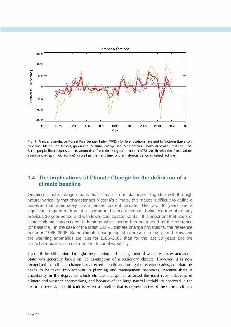
Fig. 7: Annual cumulative Forest Fire Danger Index (FFDI) for five locations relevant to Victoria (Laverton, blue line; Melbourne Airport, green line; Mildura, orange line; Mt Gambier (South Australia), red line; East Sale, purple line) expressed as anomalies from the long-term mean (1973–2015) with the five stations average overlay (thick red line) as well as the trend line for the historical period (dashed red line). ............................................................ 16
Fig. 8: Frequency distribution of 30-year anomalies of mean temperature (left, anomalies in °C relative to the 1911–2014 mean) and rainfall (right, in percentage terms relative to the

CLIMATE CHANGE SCIENCE AND VICTORIA
vii
1900–2014 mean), averaged across the three Victorian regions (Murray Basin top, South-West region middle and South-East region bottom). Shown are annual results (green bars) and results for the cool (blue bars) and warm (red bars) seasons. Anomalies for the most recent 30-year period (1985–2014) are indicated by coloured stars while anomalies for the reference period for the projections (1986–2005) are indicated by coloured arrows. Note: the warm season rainfall anomaly for the 1986–2005 period (red arrow in top left panel) was never observed amongst all possible 30 years periods. .............................................. 18
Fig. 9: Sketch of the mean meridional circulation (MMC) across the Southern Hemisphere; H and L denote regions of high and low pressure at the surface; A, B, C and D denote features discussed in Section 2.1; E shows time series of 11-year running mean of global surface temperature (black) and STR intensity (red); F shows map of the correlation between annual rainfall and STR intensity; G shows April–July rainfall decile map for the period 1986–2015. (Adapted from CSIRO and BoM 2012). ................................................ 20
Fig. 10: Annual cycle of the correlation coefficients between the subtropical ridge (STR) intensity (left) and position (right) and rainfall for the three regions of Victoria (left Y-axis, Murray Basin in green, South-West region in red and South-East region in blue). Mean values of the subtropical ridge are shown as blue bars (right Y-axis), for intensity (in hPa, left panel) and position (latitude in degrees south, right panel). Higher negative values above the dashed lines are significant at a 99% significance level. Rainfall values are based on the Bureau of Meteorology operational 5 km gridded monthly data from 1900 to 2014 and subtropical ridge values are computed from de-trended data using the Drosdowsky (2005) methodology. ....................................................................................... 21
Fig. 11: Annual cycle of the correlation coefficients between the tropical tripole index and rainfall for the three regions in Victoria (left Y-axis, Murray Basin in green, South-West region in red and South-East region in blue). Monthly standard deviations of the tripole index are shown as blue bars (right Y-axis, in °C). Negative correlations values above the dashed line are significant at the 99% significance level. Rainfall values are based on the Bureau of Meteorology operational 5 km gridded monthly data from 1900 to 2014 and tripole values are computed from de-trended HadISST data (reference) using Timbal and Hendon (2011) methodology. ........................................................................................................................ 24
Fig. 12: Annual cycle of the correlation coefficients between the Southern Annular Mode (SAM) and rainfall for the three regions in Victoria (left Y-axis, Murray Basin in green, South-West region in red and South-East region in blue). Monthly linear trends of the SAM index are shown as blue bars (right Y-axis, normalised values). Negative (positive) values above (below) the dashed line are significant at the 99% significance level. Rainfall values are based on the Bureau of Meteorology operational 5 km gridded monthly data from 1900 to 2014 and the SAM index is from Marshall (2003). ............................................................... 25
Fig. 13: Large-scale climate features of relevance to local climate in Victoria. Thick arrows show the influences each climate mode has upon either synoptic weather types affecting Victoria or another climate mode. Thin arrows indicated wind directions associated with certain synoptic weather types. ....................................................................................................... 27
Fig. 14: The annual cycle of temperature (left panels), MSLP (middle panels) and rainfall (right panels) for the three regions in Victoria, (Murray Basin top row, South-West region middle row and South-East region bottom row) as simulated by the CMIP5 models (grey lines) computed for the baseline period of 1986–2005. Model ensemble mean is shown in black and the observed climatology over the same period in brown. Rainfall and temperature observations are from the Bureau of Meteorology operational gridded observations and MSLP observations are from HadSLP2 (Allan and Ansell 2006). ....................................... 31
Fig. 15: Combined mean annual cycles (letters denote the initial of each calendar month) of the intensity (STR-I) and position (STR-P) index of the STR for the period 1948–2002 (left panel) as indicated using observations from the Bureau of Meteorology (BOM, blue curve;
CLIMATE CHANGE SCIENCE AND VICTORIA
viii
Drosdowsky 2005), the NCEP/NCAR reanalyses (NNR, light blue curve), the multi-model mean of CMIP3 models (green curve; Kent et al. 2013; the reference period here is 1948–1974) and the multi-model mean of CMIP5 models (red curve; Grose et al. 2015b). Correlation coefficients (right panel) between STR-I and rainfall for southeastern Australia (a larger region encompassing Victoria) for 1948–2002, from 35 CMIP5 models (grey), the ensemble mean (red), and the observed relationship using the Bureau of Meteorology operational gridded rainfall (black). (Source: Grose et al. 2015b) ....................................... 32
Fig. 16: Annual cycle of tripole index variability (standard deviation in °C, top panel) and relationship with rainfall across Victoria (correlation coefficient, bottom panel) for the observations (black line), 36 CMIP5 models (grey lines) and the ensemble mean (red line). The dashed line indicates the 99% confidence level. Rainfall observations are from the Bureau of Meteorology operational gridded rainfall; all quantities are computed for the baseline period of 1900–2005. ............................................................................................. 33
Fig. 17: An example table based on the outputs from the Climate Futures web tool showing results relevant for the South-West of Victoria when assessing plausible climate futures for 2060 under the RCP8.5 emission pathway, as defined by simulated changes in winter rainfall (% change) and temperature (°C of warming). (Source: www.climatechangeinaustralia.gov.au) ................................................................................ 38
Fig. 18: Time series (top left panel) of annual average surface air temperature (°C) for Victoria from 1911 to 2090, as simulated by CMIP5 models relative to the 1950–2005 mean for the RCP8.5 scenario. The central line is the median value, and the shading is the 10th and 90th percentile range of 20-year means (inner dark) and single year values (outer light). The grey shading indicates the period of the historical simulation, while the future scenario (RCP8.5) is shown with shading in purple. Observations from the Bureau of Meteorology gridded temperature dataset (brown line) and projected values from a typical model are shown (purple line). Bar plots show the projected range for seasonal change in daily maximum and minimum temperature for 2080–99 with respect to 1986-2005 for RCP2.6 (green), RCP4.5 (blue) and RCP8.5 (purple) across the three Victorian regions (top right: Murray Basin; bottom left: South-West Victoria; bottom right: South-East Victoria). Natural climate variability is represented by the grey bars. .............................................................. 40
Fig. 19: Annual mean surface temperature (°C), for the present (a) and for 2090 using GCM projected warming (b) and the statistical downscaling of GCMs (c). The 15 and 20 °C contours are shown with solid black lines; in (b) and (c) the same contours from the original climate are plotted as dotted lines. Observed temperature values are based on the Bureau of Meteorology operational 5 km gridded monthly data from 1986 to 2005. The future case is using the median change at 2090 under the RCP8.5 scenario from all CMIP5 models (b) and for the 22 models for which the SDM was applied (c). Results were produced on a 5 km grid and averaged over a 0.25° grid. ........................................................................... 42
Fig. 20: Projected changes in the number of days of warm spells (see text for definition of variables) by 2090 (2080–2099) for the Murray Basin cluster (left panel) and the Southern Slopes cluster (right panel). Results are shown for RCP4.5 (blue) and RCP8.5 (purple) relative to the 1986–2005 mean. The central line is the median value, and the shading is the 10th and 90th percentile range. Natural climate variability is represented by the grey bars. (Source: Timbal et al. 2015a, Grose et al. 2015a). ..................................................... 43
Fig. 21: Annual cycle of the number of potential frost days per month averaged over the Murray Basin cluster for two 20-year future periods shown in red, 2030 (left panel) and 2090 (right panel), as simulated by 22 statistically downscaled CMIP5 models for the RCP8.5 scenario. The central line is the median value, and the shading shows the 10th and 90th percentile range. The historical record (1950–2005) is shown by the black line and shading respectively. The observed values from the Bureau of Meteorology operational gridded dataset is shown by the dashed purple line. ........................................................................ 43

CLIMATE CHANGE SCIENCE AND VICTORIA
ix
Fig. 22: Time series (top left panel) of annual average rainfall (%) for Victoria from 1900 to 2090, as simulated by CMIP5 models relative to the 1950–2005 mean for the RCP8.5 scenario. The central line is the median value, and the shading shows the 10th and 90th percentile range of 20-year means (inner dark) and single year values (outer light). The grey shading indicates the period of the historical simulation, while the future scenario (RCP8.5) is shown with purple shading. Observations from the Bureau of Meteorology operational gridded rainfall dataset (brown) and projected values from a typical model (purple) are shown. Bar plots show the projected range for mean rainfall (change in percentage term) for 2080–99 with respect to 1986–2005 for RCP 2.6 (green), RCP4.5 (blue) and RCP8.5 (purple) across the three Victorian regions (top right: Murray Basin; bottom left: South-West Victoria; bottom right: South-East Victoria) for the CMIP5 models (GCM) and for the statistical downscaling (SDM) of 22 of the CMIP5 models (only for RCP4.5 and 8.5). Natural climate variability is represented by the grey bars. .................... 45
Fig. 23: Projected changes in mean rainfall, the magnitude of the annual maximum 1-day rainfall and the magnitude of the 20-year maximum return value for the 1-day rainfall, for 2090 (see text for definition of variables) for the Murray Basin cluster (left panel) and the Southern Slopes cluster (right panel). Relative rainfall anomalies are given as a percentage relative to the 1986–2005 mean for the RCP4.5 (blue) and RCP8.5 (purple) scenarios. The central line is the median value, and the shading is the 10th and 90th percentile range. Natural climate variability is represented by the grey bars. (Source: Timbal et al. 2015a, Grose et al. 2015a). ............................................................................................................. 47
Fig. 24: Change in snowfall for two grid boxes in the Bureau of Meteorology operational 5 km gridded observations, corresponding to a lower alpine elevation consistent with the current snowline (left panels) and for the highest elevation in the gridded observations (right panels). Future projections are provided from 2006 onward for the RCP8.5 (top row) and RCP4.5 (bottom row) scenarios. Each panel shows the model ensemble median (thick line), the 10th and 90th percentile of annual snowfall (light shading) and the 10th and 90th percentile of the 20-year mean snowfall (dark shading), operational 5 km gridded observations (brown line) and an example of a possible future time series (light purple) from a single model (ACCESS-1.0). (Source: CSIRO and BoM 2015) ............................... 48
Fig. 25: Time series for the Murray Basin cluster annual average MSLP (hPa), as simulated by CMIP5 models relative to the 1950–2005 mean for RCP8.5 (left). The central line is the median value, and the shading shows the 10th and 90th percentile range of 20-year means (inner dark) and single year values (outer light). The grey shading indicates the period of the historical simulation, while the future scenario is shown with purple shading. HadSLP2 observations are shown in brown and projected values from a typical model are shown into the future in purple. Bar plots (right) show seasonal changes (hPa) for southern Australia (from Western Australia to South-Eastern Australia) for 2080–2099 with respect to 1986–2005 for RCP2.6 (green), RCP4.5 (blue) and RCP8.5 (purple). The central line is the median value, and the shading is the 10th and 90th percentile range. Natural climate variability is represented by the grey bars. (Source: Timbal et al. 2015a) ......................... 50
Fig. 26: GCM simulations of the annual cycle of STR intensity (STR-I) and position (STR-P) for the historical period (1948–2002; light red) and for the middle (2040–2059; dark red) and end (2080–2099; black) of the 21st century under the RCP8.5 scenario. Months are denoted by their initial letter. (Source: Grose et al. 2015b). ................................................ 50
Fig. 27: CMIP5 simulated changes in drought based on the Standardised Precipitation Index (SPI) for the Murray Basin cluster (top panels) and the Southern Slopes cluster (bottom panels). The multi-model ensemble results show the percentage of time in drought (i.e. for SPI less than –1) (left panels), duration of extreme drought (middle panels) and frequency of extreme drought (right panels) for each 20-year period centred on 1995, 2030, 2050, 2070 and 2090 under RCP2.6 (green), RCP4.5 (blue) and RCP8.5 (purple). Natural climate
CLIMATE CHANGE SCIENCE AND VICTORIA
x
variability is represented by the grey bars. See CSIRO and BoM (2015), chapter 7.2.3 for definition of drought indices. (Source: Timbal et al. 2015a, Grose et al. 2015a). ................ 53
Fig. 28: Projected changes by 2090 in (a) solar radiation (%), (b) relative humidity (%, absolute change) and (c) wet-environmental potential evapotranspiration (%) for the Murray Basin cluster (top panels) and the Southern Slopes cluster (bottom panels). The bar plots show seasonal projections with respect to the 1986–2005 mean for RCP2.6 (green), RCP4.5 (blue) and RCP8.5 (purple). Natural climate variability is represented by the grey bars. (Source: Timbal et al. 2015a, Grose et al. 2015a). .............................................................. 55
Fig. 29: Projected change in seasonal soil moisture (left) and annual runoff (right) (Budyko method—see text) for the Murray Basin cluster (top panels) and the Southern Slopes cluster (bottom panels). Anomalies are given for 2080–2099 in percentage term with respect to the 1986–2005 mean for RCP4.5 (blue) and RCP8.5 (purple). Natural climate variability is represented by the grey bars. (Source: Timbal et al. 2015a, Grose et al. 2015a). ................................................................................................................................. 56
Fig. 30: Observed and projected relative sea level change (metre) relative to 1993–2010 for Stony Point, Victoria. The observed tide gauge sea level records are indicated in black, with the satellite record (since 1993) shown in mustard and the tide gauge reconstruction (which has lower variability) shown in blue. Multi-model mean projections are shown for the RCP8.5 and RCP2.6 scenarios (thick purple and olive lines) as well as RCP4.5 and RCP6.0, with uncertainty ranges shown by the purple and olive shaded regions from 2006–2100. The mustard and blue dashed lines are estimates of inter-annual variability in sea level (i.e. likely uncertainty range for the projections) and indicate that individual monthly averages of sea level can be above or below longer term averages. Note that the ranges of sea level rise should be considered likely (at least 66% probability) and that if a collapse in the marine based sectors of the Antarctic ice sheet were initiated, these projections could be several tenths of a metre higher by late in the century. (Source: Grose et al. 2015a). .. 60

CLIMATE CHANGE SCIENCE AND VICTORIA
Page 1
FOREWARD
This report summarises the state of the science regarding the climate of Victoria, its variability,
ongoing trends and projected future changes in response to continued anthropogenic forcings. It
is based primarily on the recently released national climate change projections for Australia’s
Natural Resource Management (NRM) regions: http://www.climatechangeinaustralia.gov.au/en/
As part of the national climate change projections for the NRM program, a technical report was
released to describe the science behind the projections (CSIRO and BoM 2015); this is an
important source of information to gain further understanding about the projections being
presented here and is often referred to in this report.
Also, as part of the release of the national climate change projections, reports were released for
eight clusters of NRM regions. Two of these reports are relevant to Victoria but include areas
outside the State boundaries: a report for the Murray Basin cluster covering part of Victoria,
New South Wales and South Australia (Timbal et al. 2015) and one for the Southern Slopes
cluster covering parts of Victoria and New South Wales and all of Tasmania (Grose et al. 2015).
For many climate variables, results from the NRM cluster reports relevant to the regions within
Victoria are presented here. For future projections of rainfall and temperature, additional results
were computed specifically for defined regions within the State of Victoria. These and the
national climate change projections are based on the international collaborative effort
coordinating and collecting a very large number of existing global model simulations of the
future climate: the Coupled Model Intercomparison Project Phase 5 (CMIP5, Taylor et al.
2012). CMIP5 results also underpin the science of the Fifth Assessment Report of the
Intergovernmental Panel on Climate Change (IPCC, 2013).
Important secondary sources of information for this report are the findings from a decade of
climate research programs dedicated to understanding the climate of the region: the South-
Eastern Australia Climate Initiative (SEACI, CSIRO 2010 and 2012) and the ongoing Victorian
Climate Initiative (VicCI, Murphy et al. 2014; Hope et al. 2015). These programs underpin the
additional work presented here regarding the understanding of climate variability and ongoing
changes. A focus of these climate initiatives has been to link climate science with hydrology in
order to deliver improved understanding of water availability. As such, these programs have
been able to deliver estimates of the impact of climate change on future streamflow—these will
be presented in a subsequent report.
Climate change analysis for Victoria is an ongoing activity. More information will be made
available in the future through the VicCI website: http://www.cawcr.gov.au/projects/vicci/
Climate change projections for Victoria based on data released by CSIRO and the Bureau of
Meteorology have also been included in the Victorian Government’s Climate-Ready
publications, released in 2015. Climatic trends have been used to highlight the impacts climate
change will have on Victoria’s regions and provides examples of how people are already
becoming climate-ready, with links to more detailed information. The Climate-Ready
publications are available at http://www.climatechange.vic.gov.au/understand

Page 2
EXECUTIVE SUMMARY
This report compiles all existing climate research findings of relevance to the State of Victoria;
it describes what is understood about the climate of the State and how it will likely evolve in the
future in response to ongoing anthropogenic forcings. For the purposes of this report the State of
Victoria was divided—by grouping the ten existing Catchment Management Authority (CMA)
areas—into three regions which are meaningful from a climatic, vegetative and hydrological
perspective: the Murray Basin, the South-West and South-East regions.
Victoria experiences a temperate climate: mean temperature ranges from 10 °C in winter to
20 °C in summer (with geographical differences); and rainfall, which is more abundant in the
southern regions, occurs predominantly in the cool season (April–October). The climate is
highly variable from year to year, particularly in summer. Victoria has experienced a warming
trend over the last century averaging 0.06 °C per decade (1911 to 2014), in line with global
warming. This warming trend is accompanied by natural climate variability on year-to-year and
decadal timescales. There has been no long-term trend in annual total rainfall over the historical
instrumental record, and this record exhibits marked decadal variability. But, split into two
seasons, warm season rainfall has increased and cool season rainfall has decreased. The cool
season rainfall deficit in relation to the long-term mean has accelerated in the second half of the
20th century and became statistically significant. This was particularly evident during the
Millennium Drought from 1997 to 2009. The Millennium Drought was the most severe
protracted drought of the instrumental record and was predominantly due to a cool season
rainfall deficit. Along with the declining trend in cool season rainfall, the State has also
experienced declining streamflows and increasing bushfire risk.
Ongoing climate change means the climate is non-stationary. Together with the high natural
variability that characterises Victoria’s climate, this makes it difficult to define a baseline that
adequately characterises current climate. The last 30 years are a significant departure from the
long-term historical record, being warmer than any previous 30-year period and with lower cool
season rainfall. It is important that users of climate change projections understand which period
has been used as the reference (or baseline) from which to measure future changes. The latest
CMIP5 climate change projections use 1986–2005 as the baseline. Some climate change signal
is present in this period. However, the warming anomalies are less for 1986–2005 than for the
last 30 years and the rainfall anomalies also differ due to decadal variability.
Victorian mean climate experiences natural variability on interannual and longer timescales in
response to a complex interplay of large-scale climatic phenomena. An understanding of these
phenomena and how they influence the climate of Victoria now and into the future, is required
to both appreciate local climate and also to predict its future evolution over a range of
timescales (e.g. seasonal and long-term changes). The transfer of excess energy from the tropics
to the pole(s) takes place via the mean meridional circulation, which controls the mean climate
of Victoria, the position of the band of high pressure systems (the subtropical ridge) and the
passage of rain-bearing weather systems. There are multiple lines of evidence showing that the
characteristics of this particular global circulation has been changing over the last 50 years, in
part due to anthropogenic forcings as well as natural fluctuations. These changes can be related
to some of the observed changes in rainfall across Victoria. On interannual timescales the
variability is often driven by remote large-scale mechanisms in the tropical oceans, in particular

CLIMATE CHANGE SCIENCE AND VICTORIA
Page 3
the Pacific Ocean where ENSO variability (El Niños and La Niñas) has a strong influence. In
addition to ENSO, the behaviour of the Indian Ocean, either in response to ENSO or
independently, plays an important role. Besides tropical modes of variability, the trajectories of
weather systems delivering rainfall across Victoria are affected by a hemispheric see-saw of
atmospheric pressures between 40°S and 65°S, called the Southern Annular Mode (SAM).
SAM acts to contract and expand the circulation of weather systems around Antarctica. This, in
turn, influences Victorian climate, with impacts dependent on the season, and varying across the
State. SAM has trended positively since the late 1950s and this may have contributed to the
observed ongoing deficit in cool season rainfall. While large-scale modes of variability are
important in understanding the observed variability of the climate of Victoria, they do not fully
explain the randomness of the weather. Therefore the local climate is never perfectly predictable
at any timescale. The randomness of weather noise also is embedded in historical climate model
runs and future climate projections, which explain why they are not deterministic in nature.
Besides the various modes of interannual variability relevant to Victorian rainfall, recent
research points to the importance of decadal variability. Particularly relevant are the change of
phase of the Inter-decadal Pacific Oscillation (IPO) in influencing the interaction between the
interannual modes, affecting the climate of Victoria, and also the long-term trends in the
expansion of the tropics and the Hadley Cell (which is a key component of the mean meridional
circulation).
Projections of future changes to the climate for Victoria presented in this report are based on
international efforts to gather all existing global climate model (GCM) simulations, as well as a
national program that delivered nation-wide climate change projections. The climate will
change in response to future human activities, the specifics of which are unknown as this stage.
Therefore the climate models are forced with plausible estimates of future greenhouses gas
concentrations according to likely socio-economic scenarios. These scenarios are known as
Representative Concentration Pathways or RCPs. In this report results are presented for several
of these scenarios, focusing on a higher scenario (RCP8.5 which is similar to a ‘business as
usual’ approach) and a lower scenario (RCP4.5 which is achievable only if substantial emission
reduction measures are put in place).
Projections of the evolution of the climate system in response to the human induced forcings are
produced using complex mathematical models representing both the atmospheric and oceanic
components of the global climate system. In order to capture the uncertainties of the future
projections of the climate, and because climate models contain limitations (especially for small-
scale features), it is best practice to make use of results from a large number of simulations from
existing climate models within the international community. The climate models underpinning
the future projections have been evaluated based on their ability to reproduce the observed past
and present climate, as well as the key mechanisms influencing the climate. These evaluations
are helpful in determining which processes the models simulate well and, therefore, in guiding
the selection of individual models for impact studies. These evaluations are made for important
surface climate variables across Victoria as well as for large-scale mechanisms known to drive
the variability of the climate of Victoria. We find that GCMs can capture large-scale aspects of
the climate well but are not designed to provide local information at scales finer than their
spatial resolution. To obtain local-scale projections, additional techniques are required to
downscale this information to a scale relevant for impact studies. Amongst the numerous
Page 4
existing approaches, this report makes extensive use of results from a statistical downscaling
model based on meteorological analogues.
The future climate projections for Victoria presented in this report are based on the recently
released Australian Climate Change projections (Climate Change in Australia Information for
Australia's Natural Resource Management Regions: Technical Report). This national program
delivered data as well as a series of reports which are useful background information in support
of this report and are available through the Climate Change in Australia website:
http://www.climatechangeinaustralia.gov.au/. In particular, the website provides methods and
tools to enable the selection of climate dataset(s) required to perform more advanced analysis of
the impact of climate change. While the national project went far beyond the scope of this
study, we provide additional and more local details of projected changes to Victoria’s climate.
Climate change projections for Victoria based on data released by CSIRO and the Bureau of
Meteorology have also been included in the Victorian Government’s Climate-Ready
publications, released in 2015. Climatic trends have been used to highlight the impacts climate
change will have on Victoria’s regions and provides examples of how people are already
becoming climate-ready, with links to more detailed information. The Climate-Ready
publications are available at http://www.climatechange.vic.gov.au/understand
Continued substantial warming for Victoria for mean, maximum and minimum temperature is
projected with very high confidence, taking into consideration the robust understanding of the
driving mechanisms of warming and the strong agreement on direction and magnitude of
change amongst GCMs and downscaling results. For the near future (2030), the mean projected
warming shows only minor differences between RCPs and reaches a median of around 1 °C in
maximum temperatures in both the cool and warm seasons with slightly smaller increases in
minimum temperatures. For late in the 21st century (2090), warming is markedly larger for
RCP8.5 reaching a median of about 4 °C above the 1986–2005 level during the warm season for
both maximum and minimum temperature and 3.5 °C during the cool season. In line with the
mean warming, hot temperature extremes are also projected to increase while frost risk is
projected to decrease.
In the near term (2030), there is high confidence that natural climate variability will remain the
major driver of rainfall changes from the climate of 1986–2005. Late in the century (2090)
under both RCP4.5 and RCP8.5, there is high confidence that cool season rainfall will continue
to decline and there is no clear leaning in the models towards either wetter or drier conditions in
the warm season. Apart from the simulated direction of future changes from GCM and
downscaling results, this assessment also takes into account the physical understanding of the
relationship between the atmospheric circulation and rainfall across Victoria—specifically, how
well the models represent this relationship, and what the projected changes in the circulation
are. The understanding of physical processes coupled with high model agreement results in high
confidence that the intensity of heavy rainfall events will increase. Snowfalls are projected to
continue to decline for all RCPs with high confidence, particularly under RCP8.5. Rainfall
changes will be driven by changes in general atmospheric circulation, in particular a broadening
of the mean meridional circulation, and accompanying changes in mean sea level pressure
(MSLP). MSLP over southern Australia is projected to increase with high confidence, mostly
during the cool season; this is driven by an increase in the strength of the well-known belt of
high pressures, the subtropical ridge, and a shift of this ridge southward consistent with the

CLIMATE CHANGE SCIENCE AND VICTORIA
Page 5
observed trend over the last 30 years. As climate models tend to underestimate the rainfall
response to changes in the position and intensity of the subtropical ridge, these models may
underestimate the projected rainfall decline in the cool season. Other large-scale drivers (e.g.
ENSO and SAM) are also projected to change and impact future rainfall projections.
Changes in mean and extreme wind are uncertain. Mean wind is likely to decrease during the
cool season while increased occurrence of more intense frontal systems and wind changes
during the warm season is possible.
Important changes are projected in the hydrological cycle. Linked to the rainfall projections,
there is medium confidence that the time spent in meteorological drought, and the frequency of
extreme droughts, will increase over the course of the century under RCP8.5. Beside the
changes in rainfall and temperature, changes in other variables will also contribute to changes in
the hydrological cycle. Small changes are projected for solar radiation and relative humidity by
2030 with clear increases seen by 2090. In particular, an increase in solar radiation is linked to
reduced cloud cover and rainfall decline in conjunction with a decrease in relative humidity.
Potential evapotranspiration is projected to increase in all seasons. As a result, soil moisture and
runoff are projected to decrease with medium confidence.
There is high confidence that climate change will result in a harsher fire-weather climate regime
in the future. However, there is only low confidence in the magnitude of the projected change to
fire weather, as this depends on rainfall projections and their seasonal variation. The summer
rainfall increase projected by some climate models, if it eventuates, would moderate the number
of severe fire-weather days, although there is very little confidence about this projection.
Sea level, which has risen around Australia at an average rate of 1.4 mm/year between 1966 and
2009, is projected to continue to rise during the 21st century (very high confidence). By 2090,
the projected range of sea level rise for the Victorian coastline is between 0.39 m and 0.84 m
under the high emissions scenario (RCP8.5). Sea surface temperature (SST) has increased
significantly across the globe over recent decades and is projected to further rise with very high
confidence. Across the coastal waters of Victoria in 2090, further warming is projected in the
range of 1.6 to 3.4 °C for RCP8.5. There is also very high confidence that the ocean pH is
expected to decrease around Australia.

Page 6
1. THE CLIMATE OF THE STATE OF VICTORIA
1.1 Defining climate regions
The State of Victoria was divided into three regions which are meaningful from a
climatic, vegetative and hydrological perspective: the Murray Basin, the South-West
and South-East regions. These regions are formed as groupings of the ten existing
Catchment Management Authority (CMA) areas.
In this report, the State of Victoria is divided into three regions (Fig. 1). The regions were
derived by grouping the ten existing Victorian Catchment Management Authorities (CMAs) or
Natural Resources Management (NRM) boundaries (which are defined by catchments and
bioregions), into three regions that are meaningful from a climatic perspective (discussed in
Section 1.2):
The Murray Basin section of Victoria (blue shading in Fig. 1) comprises an area to the north
of the Great Dividing Range (GDR), encompassing the Victorian section of the larger
Murray Basin NRM Cluster. This includes the Mallee, Wimmera, North Central, Goulburn
Broken and North East CMA regions;
South-West Victoria (red shading in Fig. 1), southwest of the GDR which includes the
Glenelg-Hopkins, Corangamite and Port Philip and Westernport CMA regions; and
South-East Victoria (green shading in Fig. 1), southeast of the GDR, which includes the
West and East Gippsland CMA regions.
Each region is characterised by distinct topographical and climatological features as described
in Section 1.2.
These three regions follow the clustering used in the NRM reports (shown by the thick coloured
boundaries in Fig. 1) but are restricted to the Victorian sections of the relevant clusters (shaded
on Fig. 1). The individual Victorian CMAs are shown by the thin black boundaries. Results are
presented using these three Victorian regions where possible (primarily for temperature and
rainfall). However for variables for which results are unavailable at this scale (most other
variables), the broader NRM clusters are used - in particular the Murray Basin cluster,
encompassing the Murray Basin region, and the Southern Slopes cluster, encompassing both the
South-West and South-East regions of Victoria.
A range of climate change impacts and adaptation challenges have been identified across
Victoria, including temperature and rainfall impacts on agriculture, water resources and other
natural assets, as well as shifting habitats for terrestrial and marine flora and fauna (Department
of the Environment 2013). Across the State, broad acre cropping and intensive agriculture,
invasive species and biodiversity management, water security, bushfire risk, alpine tourism and
coastal inundation are priorities for the natural resource management and planning community.

CLIMATE CHANGE SCIENCE AND VICTORIA
Page 7
Fig. 1: The three climatic regions identified across the State of Victoria: Murray Basin (blue shading), the
South-West of Victoria (red shading) and the South-East of Victoria (green shading) based on boundaries
of individual CMA subregions (thin black lines). Cluster regions used for the latest national projections for
Australia (CSIRO and BoM 2015) of relevance to Victoria are indicated by coloured boundaries: the
Murray Basin cluster (thick blue line), and the Southern Slopes cluster encompassing the South-West of
Victoria (thick red line) and South-East of Victoria (thick green line). The regional topography is shown in
the background shading. Black circles indicate major towns for each CMA subregion, fire data stations are
shown by purple triangles (see Sections 1.3 and 4.6) and Stony Point, used as an example for sea level
rise, is shown by a blue square (see Section 4.7).
1.2 Regional mean climate
Victoria experiences a temperate climate: mean temperature ranges from 10 °C in
winter to 20 °C in summer (with geographical differences); and rainfall, which is more
abundant in the southern regions, occurs predominantly in the cool season (April-
October). The climate is highly variable from year to year, particularly in summer.
The State of Victoria, located at latitudes 34–38°S, is within the ‘extra-tropics’ or ‘mid-
latitudes’ of the global climate system, generally falling between the subtropical ridge (STR) of
high pressure at approximately 30–40°S (the descending arm of the Hadley Cell—see Section
2.1 for further details) and the northern edge of the so called ‘Roaring Forties’ of westerly
circulation in 40–50°S. As such, the State is influenced by a number of synoptic-scale and
large-scale phenomena, further discussed in Section 2.

Page 8
Fig. 2: Average characteristics of monthly rainfall (bars, right axis) and temperature (lines, left axis; mean
in red, maximum in blue and minimum in green, as well as the annual mean temperature in the dashed
line) over 1900–2014 for rainfall and 1911–2014 for temperature for the three regions of Victoria: Murray
Basin (top), South-West region (middle) and South-East region (bottom). Temperature and rainfall data are
from the Bureau of Meteorology operational 5 km gridded monthly data.

CLIMATE CHANGE SCIENCE AND VICTORIA
Page 9
According to the Bureau of Meteorology records, annual mean temperatures across the State
range from around 12.6 °C in the South-East region to 14.7 °C in the inland Murray Basin
region (Fig. 2) with much larger spatial variability around individual locations. The South-West
and South-East regions, extending to the coast, experience relatively temperate, maritime
climates while the more inland Murray Basin region has a slightly warmer climate with larger
diurnal (the difference between minimum and maximum) and seasonal (the difference between
mid-summer and mid-winter maximum, mean and minimum) temperature ranges.
Total rainfall is larger in the South-East (917 mm/year) and South-West (730 mm/year) regions
compared to the drier Murray Basin region (562 mm/year); larger and smaller values are
recorded around the State at individual locations. The annual cycle of rainfall averaged across
the northern part of the State shows the dominance of the cool season rainfall (top panel in
Fig. 2). In this report, the ‘cool season’ is defined as the period for which the monthly long-term
temperature average is below the annual average. Across the State, the cool season is April to
October. The ‘warm season’ correspondingly is November to March. In general, a winter-
dominated seasonal cycle of rainfall occurs in the northern and western part of the State (May–
October peak), with a more uniform seasonal cycle in the eastern part of the State (Fig. 2).
Climate anomalies such as droughts and floods are a common feature of the Australian climate,
and Victoria is no exception. Their occurrences are partly explained by influences of well-
known large-scale natural modes of climate system variability (CSIRO 2012). These modes and
their relevance to Victorian climate are described in more detail in Section 2. It is important to
understand that these known modes, combined or individually, cannot explain the majority of
year-to-year variability—a large part of the variability is due to the randomness of weather
systems or as-yet unknown climate modes. Year-to-year standard deviations of monthly total
rainfall averaged across the State are consistently between 22 and 29 mm per month (Fig. 3).
When divided by the mean rainfall and expressed in percentage terms (three coloured lines in
Fig. 3), they tend to be lower for spring months, when modes such as the El Niño–Southern
Oscillation (ENSO) and the Indian Ocean Dipole (IOD) have the largest impact on Australian
climate (see Section 2.2). This indicates that cool season rainfall is more reliable than warm
season rainfall. Furthermore, rainfall in the Murray Basin region is more variable almost all year
around than for the two southern regions (Fig. 3).

Page 10
Fig. 3: Annual cycle of the standard deviation (STD) of monthly rainfall in mm (blue bars, right axis shown
for the entire State) and divided by the mean monthly rainfall expressed in percentage terms (coloured
lines, left axis, computed for the three regions). All values are based on rainfall from the Bureau of
Meteorology operational 5 km gridded monthly data from 1900 to 2014.
1.3 Trends and variability of the regional climate
Victoria’s warming trend over the last century has averaged 0.06 °C per decade (1911–
2014), in line with global warming. This warming trend is accompanied by natural
climate variability on year-to-year and decadal timescales. There has been no long-
term trend in annual total rainfall over the historical instrumental record, and this record
exhibits marked decadal variability. When split into two seasons, warm season rainfall
has increased and cool season rainfall has decreased. The cool season rainfall deficit,
in relation to the long-term mean, has accelerated in the second half of the 20th
century and became statistically significant. This was a significant factor in the
Millennium Drought from 1997 to 2009. The Millennium Drought was the most severe
protracted drought of the instrumental record and was predominantly due to a cool
season rainfall deficit. Along with the declining trend in cool season rainfall, the State
has also experienced declining streamflows and increasing bushfire risk.
Surface air temperatures in Victoria have been increasing by about 0.06 °C per decade (Table 1)
since national records began in 1911 (Fig. 4). Daytime maximum temperatures have risen slightly
more (0.07 °C per decade) than overnight minimum temperatures (0.05 °C per decade). All trends
are highly statistically significant for all durations considered (100, 50 and 30 years) and across all
parts of the State. The warming is fairly uniform across the three regions of the State (Table 1)
with lower warming in the South-West region and higher warming in the Murray Basin region.
The warming across the State is broadly in keeping with global temperature changes, with the rate
of warming increasing in the most recent part of the historical period; this can be seen in a
comparison of the 1911–2014 period, the last 50 years and the last 30 years’ trends (Table 1). As a
result, trends computed over the last 30 years are substantially larger, in particular for daily
maximum temperature and for the warm season (up to 0.63 °C per decade, Table 1).

CLIMATE CHANGE SCIENCE AND VICTORIA
Page 11
Tmax Victoria MB SW SE Tmin Victoria MB SW SE
Annual
Mean
0.07**
0.20**
0.45**
0.06**
0.22**
0.50**
0.09**
0.17**
0.37*
0.06**
0.16**
0.41**
Annual
Mean
0.05**
0.11**
0.16*
0.03*
0.08
0.13
0.08**
0.12**
0.17*
0.09**
0.20**
0.28*
Cool
Season
0.06**
0.18**
0.32**
0.06**
0.20**
0.37**
0.08**
0.15**
0.22*
0.06**
0.14**
0.28**
Cool
Season
0.03*
0.08
0.00
0.01
0.04
-0.08
0.06**
0.11**
0.05
0.07**
0.19**
0.18*
Warm
Season
0.07**
0.22**
0.63**
0.06*
0.25**
0.67**
0.10**
0.19*
0.58**
0.07**
0.18*
0.58**
Warm
Season
0.08**
0.15*
0.40**
0.05**
0.13*
0.42**
0.10**
0.13*
0.33*
0.13**
0.21**
0.42**
Table 1: Linear trends computed for daily maximum (Tmax; left) and minimum (Tmin; right) surface
temperature (°C/decade) for the State average and the three regions (MB; Murray Basin, SW; South-West
and SE; South-East), annually and for the cool and warm seasons. In every case trends are provided for
the full record (1911– 2014, top row), the last 50 years (1965–2014, middle row) and the last 30 years
(1985–2014, bottom row). Statistical significance of trends at the 95% level is indicated with * and at the
99% level with **. Cooling trends are shown in blue.
Fig. 4: 11-year running means of Victoria average daily minimum (blue lines) and maximum (red lines) air
temperature as anomalies (°C) relative to the 1911–2014 average; solid lines show the April to October
(cool) seasonal average and dashed lines show the November to February (warm) seasonal average.
These values are based on the Bureau of Meteorology operational 5 km gridded monthly temperature data
from 1911 to 2014. The black line shows the global average temperature anomalies (relative to the 1961–
1990 reference period) from the Climatic Research Unit website (HadCRUT4, Morice et al. 2012).

Page 12
It is worth noting that the lower rate of warming across Victoria in the early part of the record
(compared to global warming), as noted in Fig. 4, is very likely in part due to a warm bias in the
gridded temperature data used in this report. Trends computed using the Bureau of
Meteorology’s newly developed Australian Climate Observation Reference Network – Surface
Air temperature (ACORN-SAT) data (Trewin 2013; Fawcett et al. 2012) are higher than the
trends obtained here using the gridded temperature dataset. However, the increased rate of
warming since the 1970s appears concomitant with the acceleration of the global warming
(black curve on Fig. 4) with marked differences due to naturally occurring decadal variability,
as expected for a small region. This is an important reminder that while the warming observed
across Victoria is primarily driven by the increase of anthropogenic greenhouse gas emissions
that are causing global warming, year-to-year and even decadal anomalies are also driven by
regional factors. For example, daily minimum temperatures increased at a slower rate than daily
maximum temperatures during the last 30 years. This is particularly true for the cool part of the
year, when the trend in minimum temperature is nil in some areas and even negative for the
Murray Basin region, being consistent with observations of increased frost in some part of the
State over the last few decades (Dittus et al. 2014). The different warming rates for maximum
and minimum temperature observed in the last 30 years are consistent with the observed rainfall
trend discussed in Section 2.2, as there is a strong relationship between rainfall reduction and an
increase in diurnal temperature range (Power et al. 1998).
Annual rainfall across the State is highly variable and exhibits a small and statistically non-
significant drying trend over the full instrumental record (1900–2014; Table 2). However,
trends strengthen when the last 50 years are considered and, with the exception of the South-
East region, strengthen even further when the last 30 years are considered (although on an
annual basis these 50 and 30 year trends are still not statistically significant). The State has
experienced some remarkable rainfall variability in the last 15 years (Fig. 5), including the
record breaking Millennium Drought which affected most of southeastern Australia, including
the Murray Basin (Leblanc et al. 2012). The rainfall anomalies during this event were
particularly large compared to previous historical droughts—for example, as discussed in
Timbal et al. (2015b) for the high rainfall hydrological catchments on both sides of the Great
Dividing Range. The Millennium Drought ended with two of the wetter years on record for
Australia in 2010–11 (Beard et al. 2011, Bureau of Meteorology 2012). However, across
Victoria, while these two years were very wet and contributed to a recovery of surface water
resources, they were not the highest on record. This arose because exceptionally high rainfalls
were limited to the northern part of the State (Bureau of Meteorology, 2012)—for 2010–11, the
2-year Victorian average was 845 mm per year, which was the third wettest 2-year period after
1973–74 (927 mm) and 1955–56 (860 mm) (Bureau of Meteorology, 2012). In addition to
seasonal totals, evidence has emerged that extreme rainfalls are also increasing across Australia,
including locations in Victoria (Gallant et al. 2014).

CLIMATE CHANGE SCIENCE AND VICTORIA
Page 13
Rainfall Victoria MB SW SE
Annual Mean
-1.6%
-9.9%
-12.9%
-0.8%
-11.2%
-15.6%
-2.4%
-9.0%
-13.7%
-2.3%
-8.0%
-6.2%
Cool Season
-7.3%
-15.8%
-26.1% *
-9.5%
-21.7%
-37.5% **
-3.9%
-10.2%
-17.0%
-5.9%
-8.5%
-9.7%
Warm Season
9.7%
1.9%
13.3%
17.6%
11.0%
30.9%
1.0%
-6.4%
-6.7%
3.3%
-7.1%
-0.6%
Table 2: Linear trends computed for rainfall for the State average and the three regions (MB; Murray
Basin, SW; South-West and SE; South-East); in every case trends are provided for the full record (1900–
2014, top row), the last 50 years (1965–2014, middle row) and the last 30 years (1985–2014, bottom row)
and are expressed as a percentage of the mean over the period considered. Statistical significance at the
95% level is indicated with * and at the 99% level with **. Drying trends are shown in red.
Fig. 5: Average Victorian observed annual rainfall anomalies in mm (red bars, from 1900 to 2014, left axis)
and the 11-year running mean (bold red line, left axis). Additionally, the 11-year running mean of the
difference between the April–October (cool season) and November–March (warm season) rainfall is
shown (bold blue line, right axis). All values are based on rainfall from the Bureau of Meteorology
operational 5 km gridded monthly data from 1900 to 2014.
The Millennium Drought was dominated by autumn and early winter rainfall declines (primarily
within the cool season); in contrast, the very wet La Niña-driven 2010–11 period was
dominated by warm season rainfall. These dry and wet events have contributed to a marked
ongoing difference between cool and warm season rainfall due to both a decline in cool season
rainfall and an increase in warm season rainfall. As was the case for the warming trend
discussed earlier, these two opposite trends in seasonal rainfall accelerated in the latter part of

Page 14
the historical period, illustrated by comparing the trends of the last 50 and 30 years with those
of 1900–2014 (Table 2). However, in contrast to temperature trends, the rainfall trends are not
statistically significant, with the exception of the last 30-year cool season rainfall trend, despite
being large in percentage terms. This is due to the high natural variability of rainfall discussed
earlier (Fig. 3). The spatial extent of the decreasing cool season rainfall (and the trend's
acceleration in the latter part of the instrumental record) is consistent across the State and is
most pronounced north of the Great Dividing Range (the Murray Basin region), and least
pronounced south of the Range, in particular in South-East Victoria (Table 2). The increasing
warm season rainfall trend is not consistent across the State and in the more recent period is
only a feature of the Murray Basin region. In this case, it is nearly as large as the cool season
rainfall decline in percentage terms, albeit from a much lower mean rainfall (381 mm for the
cool season versus 180 mm for the warm season on average across the Murray Basin region,
Fig. 1).
Streamflow data have been compiled by the Bureau in the Hydrological Reference Stations
(HRS) dataset (Turner et al. 2012). The HRS dataset catchments were chosen to track the
influence of climate change on streamflow and, hence, are relatively unimpaired by human
activities and located generally at the headwaters of major drainage basins (Sinclair Knight
Merz 2010). Twenty-seven catchments across Victoria, selected from the HRS dataset by
Fiddes and Timbal (2016a), have experienced declines in the total streamflow received per year
since the 1970s (Fig. 6), with most of the decline experienced since the 1990s. This decline in
annual streamflow is primarily driven by cool (April–October) season rainfall decline, and is
coincident with the traditional filling season for water storages in Victoria. The catchments in
close proximity to the Great Dividing Range show weaker trends than the lower elevation
catchments further away from the range. During the warm season there is a large increasing
trend in percentage terms. However, this is small in absolute terms, and warm season
streamflow does not compensate for the cool season decline. On both annual and seasonal time
scales, linear trends in streamflow decline are highly related to the runoff via a log-linear
relationship: the catchments that generate higher runoff north of the Great Dividing Range, in
the Murray Basin region, experienced the least effect (in percentage terms) of the negative
rainfall trend since the 1970s (Fig. 6). Hence, the difference in streamflow response during the
Millennium Drought or the reduction since the 1970s (e.g. stronger decline in the northwest of
the State compared to the northeast) has more to do with the catchment's physical properties and
mean runoff than the magnitude of the changes in cool season rainfall (Fiddes and Timbal
2016a).
Trends in climatic variables are also reflected in trends in the risk of bushfires. Bushfire
occurrence depends on four ‘switches’: 1) ignition, either human-caused or from natural sources
such as lightning; 2) fuel abundance or load; 3) fuel dryness, where lower moisture contents are
helpful for fire propagation and; 4) suitable weather conditions for fire spread, generally hot,
dry and windy (Bradstock 2010). The settings of most of these switches depend on
meteorological conditions across a variety of timescales and, given this strong dependence on
the weather, climate change will have a significant impact on future fire weather. Fire weather is
estimated here using the McArthur Forest Fire Danger Index (FFDI, McArthur 1967). This
index includes a drought factor that depends on both long-term and short-term rainfall.
Therefore, temperature, relative humidity and wind speed are direct inputs into the calculation
of FFDI. Fire weather is considered ‘severe’ when the FFDI index exceeds 50. Climatological

CLIMATE CHANGE SCIENCE AND VICTORIA
Page 15
time series of FFDI are limited to locations where long records exist for the meteorological
variables used in computing the FFDI. At five stations across Victoria (either within the State or
close to State boundaries), historical records are sufficient to evaluate the evolution of FFDI
from 1973 to 2015 (Table 3 and Fig. 7). These locations provide a broad indication of fire
danger in the surrounding area, covering different climate zones, but not capturing the alpine
regions of Victoria. At all locations but one, the FFDI has been increasing during this period,
which gives a State-wide significant increase. This increase is most significant in the spring
season leading to an overall lengthening of the fire season. At the tail of the distribution of fire
danger, the number of days when FFDI reaches the severe threshold (above 50) has seen a
significant increase, larger than the increase in annual cumulative FFDI (Table 3).
Fig, 6: Decadal linear trends (expressed as a percentage of the 1977–2012 mean) for annual streamflow
for the period of 1977–2012 across a selection of Victorian catchments (left panel). Trends significant at
the 90% (thick grey borders) and 95% (thick black borders) confidence levels are highlighted. The
relationship of the trends’ magnitude across the 27 catchments to the log-transformed runoff in these
catchments is shown for the annual mean and the cool and warm seasons (right panel). Compared to
rainfall, the seasons for streamflow are shifted by a month: cool is May to November and warm is
December to April. All streamflow data are extracted from the Hydrological Reference Stations data
assembled by the Bureau of Meteorology. (Source: Fiddes and Timbal 2016a).
Station
Mean annual
cumulative
FFDI
(1981-2010)
Linear trend in
percentage of the
mean (1973-
2015)
Averaged number
of days per year
with
FFDI > 50 (severe)
Linear trend in
number of days
for FFDI > 50
(1973-2015)
Melbourne Airport 2553 37% 2.7 4.6
Laverton 2208 20% 1.7 1.0
Mt Gambier 2026 17% 1.6 3.6
Mildura 5488 42% 7.2 8.6
East Sale 1849 21% 0.5 0.0
Station average 2824 28% 2.7 3.6
Table 3: Individual station and average composite of key statistics of the Forest Fire Danger index (FFDI):
mean annual cumulative FFDI and the linear trends of that quantity expressed as a percentage of the
mean value for the full available record (1973–2015); number of days per years of severe FFDI (above
50); and the linear trend of that quantity. N.B: FFDI year are reported from 1st of July to end of June (i.e.
2015 FFDI is from 1 July 2014 to 30 June 2015).
Page 16
Fig. 7: Annual cumulative Forest Fire Danger Index (FFDI) for five locations relevant to Victoria (Laverton,
blue line; Melbourne Airport, green line; Mildura, orange line; Mt Gambier (South Australia), red line; East
Sale, purple line) expressed as anomalies from the long-term mean (1973–2015) with the five stations
average overlay (thick red line) as well as the trend line for the historical period (dashed red line).
1.4 The implications of Climate Change for the definition of a climate baseline
Ongoing climate change means that climate is non-stationary. Together with the high
natural variability that characterises Victoria’s climate, this makes it difficult to define a
baseline that adequately characterises current climate. The last 30 years are a
significant departure from the long-term historical record, being warmer than any
previous 30-year period and with lower cool season rainfall. It is important that users of
climate change projections understand which period has been used as the reference
(or baseline). In the case of the latest CMIP5 climate change projections, the reference
period is 1986–2005. Some climate change signal is present in this period. However
the warming anomalies are less for 1986–2005 than for the last 30 years and the
rainfall anomalies also differ due to decadal variability.
Up until the Millennium Drought the planning and management of water resources across the
State was generally based on the assumption of a stationary climate. However, it is now
recognised that climate change has affected the climate during the recent decades, and that this
needs to be taken into account in planning and management processes. Because there is
uncertainty in the degree to which climate change has affected the most recent decades of
climate and weather observations, and because of the large natural variability observed in the
historical record, it is difficult to select a baseline that is representative of the current climate

CLIMATE CHANGE SCIENCE AND VICTORIA
Page 17
while also encompassing an appropriate range of natural climate variations. The
recommendation of the World Meteorological Organization (WMO) is to use a period of at least
30 years to define a reference period. It is therefore of interest to evaluate how unusual the last
30 years (1985–2014) of rainfall and temperature have been across the three Victorian regions
(Fig. 8). It emerges that for all regions, for both warm and cool seasons and the annual mean,
the last 30 years have been the warmest of any 30-year period in the historical record (e.g.
coloured bars with stars in left column of Fig. 8 are furthest to the right). For rainfall, in the last
30 years the cool season has been the driest 30-year period observed in the historical record for
the Murray Basin and South-West regions (e.g. blue bars with stars in the right column of Fig. 8
are further to the left); however this is not the case for annual or warm season rainfall. From this
analysis, it appears that any approach which samples the full historical record to estimate the
likelihood of a particular outcome may be biased with respect to the current state of the climate
in Victoria.
It is also important that users of future climate change projections understand from which
reference period differences are computed. In this document, in line with the latest IPCC report
(IPCC 2013) and the Technical Report for the National Climate Change Projections (CSIRO
and BoM 2015), climate change projections for the 21st century are calculated as changes
relative to the 1986–2005 baseline period. For the three Victorian regions, annual, cool and
warm season rainfall anomalies are indicated for this baseline period in Fig. 8 with coloured
arrows. For the two southern regions of Victoria, rainfall anomalies for the IPCC baseline
period are relatively similar to those of the last 30 years (1985–2014); for the Murray region,
however, there is a difference of 6–7% for the cool and warm season anomalies with the 1985–
2014 period being wetter than the last 30 years. These differences reflect the high decadal
variability in rainfall. However, because of the more consistent longer term trends in
temperature, average annual temperatures for the 1986–2005 baseline period are usually only
0.1 to 0.4 °C cooler then the last 30 years anomalies. Therefore, while consistent with
international best practice, choosing 1986–2005 as the reference period for the future
projections introduces some differences compared to the climate as defined for the last 30 years.
These differences are common when switching between baseline periods, and it is
recommended that this be clearly understood when making use of the projections information.
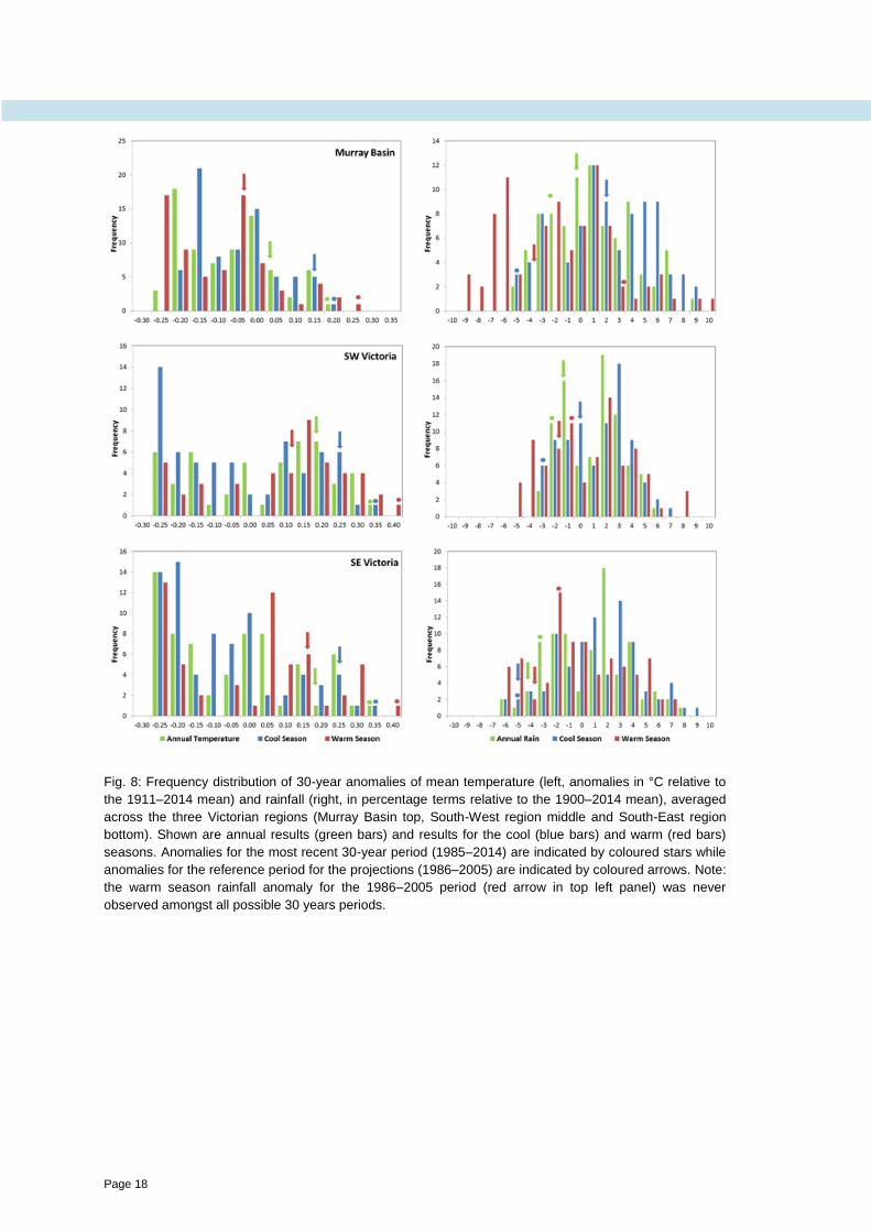
Page 18
Fig. 8: Frequency distribution of 30-year anomalies of mean temperature (left, anomalies in °C relative to
the 1911–2014 mean) and rainfall (right, in percentage terms relative to the 1900–2014 mean), averaged
across the three Victorian regions (Murray Basin top, South-West region middle and South-East region
bottom). Shown are annual results (green bars) and results for the cool (blue bars) and warm (red bars)
seasons. Anomalies for the most recent 30-year period (1985–2014) are indicated by coloured stars while
anomalies for the reference period for the projections (1986–2005) are indicated by coloured arrows. Note:
the warm season rainfall anomaly for the 1986–2005 period (red arrow in top left panel) was never
observed amongst all possible 30 years periods.

CLIMATE CHANGE SCIENCE AND VICTORIA
Page 19
2. LARGE-SCALE INFLUENCES ON VICTORIAN CLIMATE
Victorian climate experiences natural variability on interannual and longer timescales in
response to a complex interplay of large-scale climatic phenomena. An understanding
of these phenomena, and how they influence the climate of Victoria now and into the
future, is required to both appreciate local climate and also to predict its future
evolution over a range of timescales (e.g. seasonal and long-term changes).
2.1 Mean meridional circulation and the subtropical ridge
The transfer of excess energy from the tropics to the pole(s) takes place via the mean
meridional circulation, which controls the mean climate of Victoria, the position of the
band of high pressure systems (the subtropical ridge) and the passage of rain-bearing
weather systems. There are multiple lines of evidence showing that the characteristics
of this particular global circulation has been changing over the last 50 years, in part
due to anthropogenic forcings as well as natural fluctuations. These changes can be
related to some of the observed changes in rainfall across Victoria.
Victoria is located under the descending arm of the Hadley Cell, which is a part of the global
mean meridional circulation (MMC) depicted in Fig. 9. This shows a north-south cross-section
through the Southern Hemisphere atmosphere above eastern Australian longitudes. The MMC is
the main mechanism by which the planet transfers excess heat received at the Equator to the
Poles. The descending arm of the Hadley Cell is tightly linked to surface high pressure systems
(H in Fig. 9), resulting in relatively warm and dry air and little rainfall. This band of high
pressure is called the subtropical ridge (STR). Rainfall over Victoria is associated with low
pressure systems observed in between high pressure systems that are associated with either mid-
latitude storm tracks (predominantly south of the STR) or cut-off lows (predominantly north of
the STR).
Further south, the ‘roaring 40s’ and ‘50s’ constitute a band of strong westerly winds and storms
that encircle Antarctica (Sturman and Tapper 1996) and are very important for Victorian climate
during the cool season. The centres of these storms in the surface westerlies are generally located
south of Australia (Simmonds and Keay 2000); however, fronts associated with these storms are
far reaching and have a large impact on Victoria. Along with cut-off lows, they are a major source
of rainfall across Victoria (Risbey et al. 2009a and 2009b, Pook et al. 2012) all year around and
especially during the cool season. During the warm season, cold fronts in south eastern Australia
bring the classic ‘cool change’—a significant change in air temperature (from warm to cool),
accompanied by a change in wind direction at the boundary of a front. Fronts are associated with
strong winds and increased fire danger (Mills 2005). Recent climatologies indicate the prevalence
of fronts as rain bearing systems, particularly cold fronts, across southern Australia (Berry et al.
2011, Simmonds et al. 2012). Any trends in observed winds are difficult to establish due to sparse
coverage of wind observations, difficulties with instruments and the changing circumstances of
anemometer sites (Jakob 2010). McVicar et al. (2012) and Troccoli et al. (2012) have reported
weak and conflicting trends in observed winds across Australia (although they considered winds
at different levels). Circumventing the surface wind observation issues, Alexander et al. (2011)
reported, using the gradient in MSLP, that storminess affecting southeastern Australia has
experienced a significant reduction during the 20th century.

Page 20
Changes have been observed in key components of the MMC affecting the climate of Victoria.
It is now well accepted that the tropics have expanded in recent decades: the edge of the tropical
tropopause (symbol A in Fig. 9) has trended poleward during the last 30 years (Lucas et al.
2012); the subtropical jet (B in Fig. 9) has decreased in intensity, while the polar front jet (C in
Fig. 9) has increased in intensity (Frederiksen et al. 2011). The position of the descending arm
of the Hadley Cell (D in Fig. 9) has also moved poleward during the last 30 years (Nguyen et al.
2013). All these large-scale changes indicate a poleward extension of the southern hemisphere
Hadley circulation (Lucas et al. 2014).
Fig. 9: Sketch of the mean meridional circulation (MMC) across the Southern Hemisphere; H and L denote
regions of high and low pressure at the surface; A, B, C and D denote features discussed in Section 2.1; E
shows time series of 11-year running mean of global surface temperature (black) and STR intensity (red);
F shows map of the correlation between annual rainfall and STR intensity; G shows April–July rainfall
decile map for the period 1986–2015. (Adapted from CSIRO and BoM 2012).
MMC expansion affects the climate across Australia and, in particular, Victoria. Intensification
of the STR (i.e. increased surface pressure) observed during the last 120 years has occurred in
conjunction with global warming of the planet (see E in Fig. 9) (Timbal and Drosdowsky 2013).
MSLP changes over southern Australia are likely to have been in part driven by human
influences (Grose et al. 2015c). Annual rainfall in much of southern Australia has a significant
negative relationship with the intensity of the STR (see F in Fig. 9), in particular across Victoria
and for cool season rainfall (Timbal and Drosdowsky 2013). The spatial extent of drying in the

CLIMATE CHANGE SCIENCE AND VICTORIA
Page 21
early part of the cool season (April to July) during the last 30 years (see G in Fig. 9) coincides
with the areas where the STR influences rainfall, and is particularly significant across Victoria.
Fig. 10: Annual cycle of the correlation coefficients between the subtropical ridge (STR) intensity (left) and
position (right) and rainfall for the three regions of Victoria (left Y-axis, Murray Basin in green, South-West
region in red and South-East region in blue). Mean values of the subtropical ridge are shown as blue bars
(right Y-axis), for intensity (in hPa, left panel) and position (latitude in degrees south, right panel). Higher
negative values above the dashed lines are significant at a 99% significance level. Rainfall values are
based on the Bureau of Meteorology operational 5 km gridded monthly data from 1900 to 2014 and
subtropical ridge values are computed from de-trended data using the Drosdowsky (2005) methodology.
During summer the STR is weaker (close to the global average mean sea level pressure of
1013 hPa) and located further south (about 40°S), while during winter it is stronger (up to
1022 hPa) and further north (about 30°S) (Fig. 10). This behaviour influences seasonal rainfall

Page 22
in Victoria with a more intense STR associated with declines in cool season rainfall,
amplified—albeit to a lesser degree—by a poleward shift of the STR, also associated with
reduced cool season rainfall. The relationship between the STR variability and Victorian rainfall
is highly consistent across the three regions and is stronger and usually highly statistically
significant during the cool season (Fig. 10). Small differences do exist across Victoria: the
relationship with the intensity of the STR is stronger in the South-West and Murray Basin
regions and weaker in the South-East region (Fig. 10) where major rainfall events are associated
with easterly systems which are not influenced by the STR.
2.2 Tropical modes of variability
Victorian climate is highly variable. On interannual timescales the variability is often
driven by remote large-scale mechanisms in the tropical oceans, in particular the
Pacific Ocean where ENSO variability (El Niños and La Niñas) has a strong influence.
In addition to ENSO, the behaviour of the Indian Ocean, either in response to ENSO or
independently, plays an important role.
The weather and climate features described in the Section 1 are modulated from year-to-year by
the main modes of natural tropical climate variability: the El Niño–Southern Oscillation
(ENSO) and the Indian Ocean Dipole (IOD). ENSO originates in the Pacific Ocean and is the
major driver of global interannual climate variability. Its link to Australian climate variability is
well established (e.g. McBride and Nicholls 1983). Under normal conditions (the ENSO
‘neutral’ phase) the Walker Circulation and Pacific sea surface temperatures (SSTs) are in
balance, with the easterly equatorial trade winds feeding moisture into the strong convection
over the West Pacific Warm Pool. This produces high rainfall over the Maritime Continent and
to the north of Australia. In other years the trade winds weaken or reverse, the Warm Pool
expands eastward and convection moves away from the Australian region. During these ‘El
Niño’ conditions, SSTs are warmer in the eastern Pacific and cooler than average around
northern Australia. As a result rainfall is often below average over much of eastern Australia. In
some other years, the trade winds strengthen, the eastern Pacific cools and SSTs around
northern Australia are warmer than average. During these ‘La Niña’ conditions convection over
northern Australia is enhanced and rainfall is often above average over eastern Australia. While
El Niño and La Niña events are natural variations in the climate system, occurring on average
every 4–7 years, ENSO also displays significant decadal variability (Power and Colman 2006).
Australia’s wettest 2-year period on record (2010–11), which ended the Millennium Drought
across southeastern Australia (including Victoria), was associated with a strong, prolonged
La Niña. The influence of ENSO on Australian rainfall is strongest in the later part of the
calendar year.
The IOD is active in the tropical Indian Ocean, influencing interannual climate variability
across tropical and extratropical Australia. The IOD is characterised by changes in SSTs off the
Sumatran coast in the eastern Indian Ocean basin and changes of the opposite sign in the
western Indian Ocean (Saji et al. 1999). Low SSTs in the east (and high in the west) form the
‘positive’ phase of the IOD and these conditions come about when southeasterly winds off
northwest Australia induce upwelling in the eastern Indian Ocean (England et al. 2006). The
IOD is usually active from May to November and is often terminated by the wind reversal
accompanying the arrival of the northern Australia monsoon (e.g. Hendon et al. 2014). A
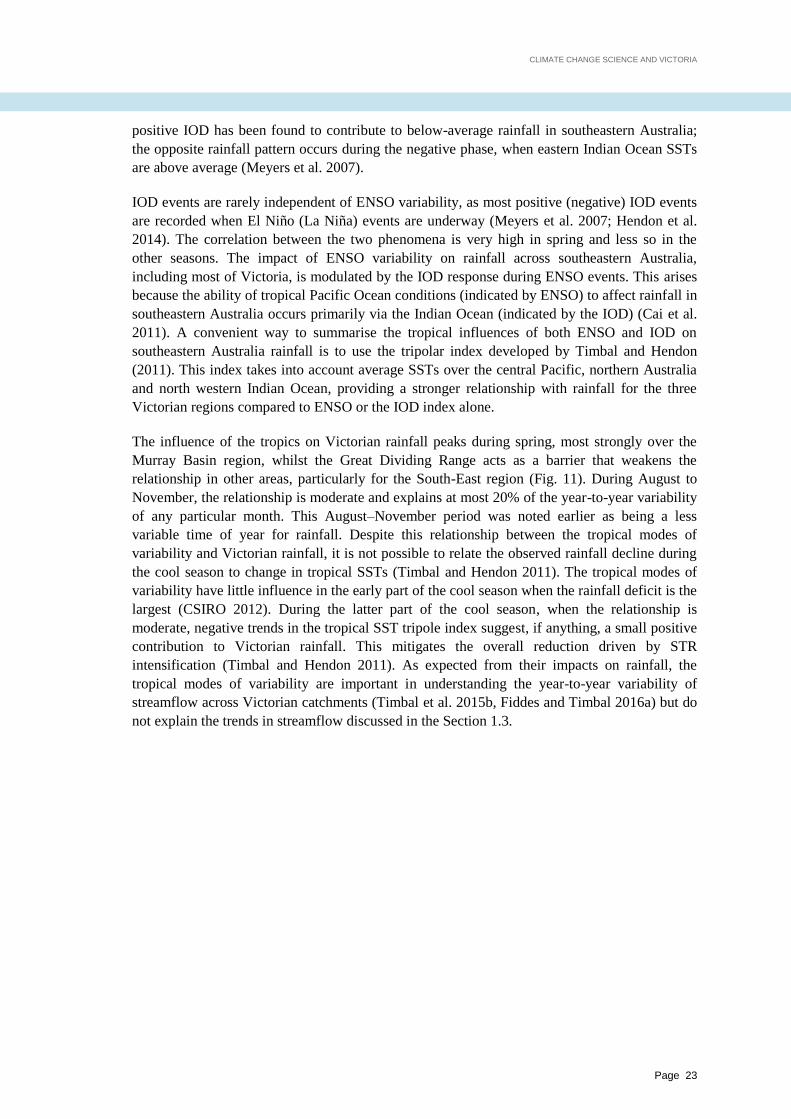
CLIMATE CHANGE SCIENCE AND VICTORIA
Page 23
positive IOD has been found to contribute to below-average rainfall in southeastern Australia;
the opposite rainfall pattern occurs during the negative phase, when eastern Indian Ocean SSTs
are above average (Meyers et al. 2007).
IOD events are rarely independent of ENSO variability, as most positive (negative) IOD events
are recorded when El Niño (La Niña) events are underway (Meyers et al. 2007; Hendon et al.
2014). The correlation between the two phenomena is very high in spring and less so in the
other seasons. The impact of ENSO variability on rainfall across southeastern Australia,
including most of Victoria, is modulated by the IOD response during ENSO events. This arises
because the ability of tropical Pacific Ocean conditions (indicated by ENSO) to affect rainfall in
southeastern Australia occurs primarily via the Indian Ocean (indicated by the IOD) (Cai et al.
2011). A convenient way to summarise the tropical influences of both ENSO and IOD on
southeastern Australia rainfall is to use the tripolar index developed by Timbal and Hendon
(2011). This index takes into account average SSTs over the central Pacific, northern Australia
and north western Indian Ocean, providing a stronger relationship with rainfall for the three
Victorian regions compared to ENSO or the IOD index alone.
The influence of the tropics on Victorian rainfall peaks during spring, most strongly over the
Murray Basin region, whilst the Great Dividing Range acts as a barrier that weakens the
relationship in other areas, particularly for the South-East region (Fig. 11). During August to
November, the relationship is moderate and explains at most 20% of the year-to-year variability
of any particular month. This August–November period was noted earlier as being a less
variable time of year for rainfall. Despite this relationship between the tropical modes of
variability and Victorian rainfall, it is not possible to relate the observed rainfall decline during
the cool season to change in tropical SSTs (Timbal and Hendon 2011). The tropical modes of
variability have little influence in the early part of the cool season when the rainfall deficit is the
largest (CSIRO 2012). During the latter part of the cool season, when the relationship is
moderate, negative trends in the tropical SST tripole index suggest, if anything, a small positive
contribution to Victorian rainfall. This mitigates the overall reduction driven by STR
intensification (Timbal and Hendon 2011). As expected from their impacts on rainfall, the
tropical modes of variability are important in understanding the year-to-year variability of
streamflow across Victorian catchments (Timbal et al. 2015b, Fiddes and Timbal 2016a) but do
not explain the trends in streamflow discussed in the Section 1.3.
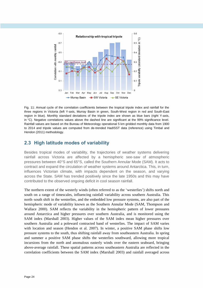
Page 24
Fig. 11: Annual cycle of the correlation coefficients between the tropical tripole index and rainfall for the
three regions in Victoria (left Y-axis, Murray Basin in green, South-West region in red and South-East
region in blue). Monthly standard deviations of the tripole index are shown as blue bars (right Y-axis,
in °C). Negative correlations values above the dashed line are significant at the 99% significance level.
Rainfall values are based on the Bureau of Meteorology operational 5 km gridded monthly data from 1900
to 2014 and tripole values are computed from de-trended HadISST data (reference) using Timbal and
Hendon (2011) methodology.
2.3 High latitude modes of variability
Besides tropical modes of variability, the trajectories of weather systems delivering
rainfall across Victoria are affected by a hemispheric see-saw of atmospheric
pressures between 40°S and 65°S, called the Southern Annular Mode (SAM). It acts to
contract and expand the circulation of weather systems around Antarctica. This, in turn,
influences Victorian climate, with impacts dependent on the season, and varying
across the State. SAM has trended positively since the late 1950s and this may have
contributed to the observed ongoing deficit in cool season rainfall.
The northern extent of the westerly winds (often referred to as the ‘westerlies’) shifts north and
south on a range of timescales, influencing rainfall variability across southern Australia. This
north–south shift in the westerlies, and the embedded low pressure systems, are also part of the
hemispheric mode of variability known as the Southern Annular Mode (SAM, Thompson and
Wallace 2000). SAM reflects the variability in the hemispheric pattern of lower pressures
around Antarctica and higher pressures over southern Australia, and is monitored using the
SAM index (Marshall 2003). Higher values of the SAM index mean higher pressures over
southern Australia and a poleward contracted band of westerlies. The impact of SAM varies
with location and season (Hendon et al. 2007). In winter, a positive SAM phase shifts low
pressure systems to the south, thus shifting rainfall away from southeastern Australia. In spring
and summer a positive SAM phase shifts the westerlies southward, allowing more tropical
incursions from the north and anomalous easterly winds over the eastern seaboard, bringing
above-average rainfall. These spatial patterns across southeastern Australia are reflected in the
correlation coefficients between the SAM index (Marshall 2003) and rainfall averaged across

CLIMATE CHANGE SCIENCE AND VICTORIA
Page 25
the three Victorian regions (Fig. 12). The largest negative relationship (positive SAM phase
correlating with less rainfall) is seen in the middle of the cool season (July) and is largest in the
South-West region. The positive relationship (positive SAM phase correlating to more rainfall)
is seen in late spring to early summer and is most prominent in the Murray Basin region. For the
South-East region, the relationship is weak and insignificant all year round.
The annual cycle of the variability of SAM is fairly even all year around (not shown); instead
the annual cycle of the linear trend of the SAM index is shown in Fig. 12. The SAM index has
been trending upward since the late 1950s with the largest trend in summer and autumn
extending into the early part of the cool season (July). For this reason, SAM is likely to have
contributed to the cool season rainfall decline, at least early in the season. This contribution is
not necessarily independent of the contribution from the STR intensification, as a trend towards
a more positive SAM implies an increase in intensity of the zonal belt of high pressure.
Fig. 12: Annual cycle of the correlation coefficients between the Southern Annular Mode (SAM) and rainfall
for the three regions in Victoria (left Y-axis, Murray Basin in green, South-West region in red and South-
East region in blue). Monthly linear trends of the SAM index are shown as blue bars (right Y-axis,
normalised values). Negative (positive) values above (below) the dashed line are significant at the 99%
significance level. Rainfall values are based on the Bureau of Meteorology operational 5 km gridded
monthly data from 1900 to 2014 and the SAM index is from Marshall (2003).
2.4 Synoptic variability or ‘weather noise’
While large-scale modes of variability are important in understanding the observed
variability of the climate of Victoria, they do not fully explain the randomness of the
weather. Therefore the local climate is never perfectly predictable at any timescale.
The randomness of weather noise is also embedded in historical climate model runs
and future climate projections from global climate models, which explains why they are
not deterministic in nature.
The term ‘synoptic variability’ refers to the high frequency (day-to-day) variability of weather
due to the passage of fronts or lows (often rain-bearing) and high pressure systems (which can
last for extended periods in the case of blocking events). The modes of variability internally
Page 26
generated by the climate system described above (either tropical, ENSO and IOD; or
extratropical, SAM) are felt on the regional climate of Victoria through their impact on the
synoptic variability. These impacts are well understood and contribute greatly to the ability to
deliver seasonal climate predictions. It is important however to remember that while these large
scale modes influence Victorian climate, for any given month they account for less than 20% of
the year-to-year variability in any part of the State (see Section 1.2). Therefore, a large part of
the naturally occurring synoptic variability is random and unpredictable: from a climatological
perspective this is referred to as ‘the weather noise’.
In addition to the frontal systems affecting southern Australian rainfall and temperatures, some
low pressure systems separated from the westerly storm track (known as ‘cut-off lows’) are
particularly important, bringing large rainfall totals to southern Australia (Pook et al. 2012). On
the Australian east coast, cut-off lows can sometimes form over the Tasman Sea, and are
commonly referred to as East Coast Lows (ECLs). These systems are responsible for some of
the more damaging natural disasters and for major flows within water catchments (Dowdy et al.
2013a). ECLs predominantly impact the eastern seaboard, east of the Great Dividing Range,
extending to the southeastern regions of Victoria. Interestingly, the large-scale modes of
variability (described above) do not appear to have a significant influence on ECL
occurrence (Dowdy et al. 2013a). As ECLs are a major contributor to southeastern Victorian
rainfall, this explains the weaker relationship between rainfall in the South-East region and the
tropical (Fig. 11) and extratropical (Fig. 12) modes of variability over large parts of the year
(Pepler et al. 2014).
2.5 Interactions between modes of variability
Besides the various modes of interannual variability relevant to Victorian rainfall, recent
research points to the importance of decadal variability. Particularly relevant are the
change of phase of the Inter-decadal Pacific Oscillation (IPO) in influencing the
interaction between the interannual modes, affecting the climate of Victoria, and also
the long-term trends in the expansion of the tropics and the Hadley Cell (which is a key
component of the mean meridional circulation).
The various modes of variability described in Sections 2.2, 2.3 and 2.4 are not independent of
one another. The ways they interact vary on decadal time scales, with a flow-on effect on
rainfall in Victoria. These variations are related to the phase of the Inter-decadal Pacific
Oscillation (IPO) (Lim et al. 2016). The IPO is a fluctuation of SSTs in the Pacific Ocean,
spatially broader than the ENSO variability, and operating on a non-regular multi-decadal
timescale; typically taking 15 to 30 years to shift from a warm to a cold phase. Unlike ENSO,
the IPO may not be a single physical ‘mode’ of variability but rather the result of several
processes with different origins. Currently, there appears to be no predictability in the phase
swings of the IPO. The most recent phase change of the IPO was in 1999, transitioning to its
cold phase (that is, cooler sea-surface temperatures in the east Pacific and warmer in the west, in
terms of a decadal mean). This is associated with reduced variability and predictability of
ENSO and, as such, impacts on seasonal prediction capabilities. A cold IPO phase means a
warming of the waters north of Australia. Thus the IPO cold phase has a similar signature to
global warming in the sea-surface temperatures north of Australia. These combined factors
enhanced recent La Niña events, which in turn fostered a strong positive SAM, further

CLIMATE CHANGE SCIENCE AND VICTORIA
Page 27
triggering greater spring and summer rainfall during 2010 (Lim and Hendon 2015a). This
relationship between ENSO and SAM is relevant in dry years as well as in wet years; the strong
drought over Victoria in the spring of 2002 has been shown to be due to both the moderate
El Niño event and the strong negative phase of SAM at that time (Lim and Hendon 2015b).
Furthermore, the phase of the IPO also influences the strength of the ENSO–IOD relationship
and modulates the spatial patterns of their teleconnections to Australian climate. For instance,
the recent cold phase of the IPO appeared to create stronger links with Victorian rainfall, despite
reducing the strengths of ENSO and IOD (Lim et al. 2016). Victorian rainfall tends to vary
more directly with ENSO indicators during wet years (La Niña) and with IOD indicators during
dry years (El Niño and subsequent positive IOD). Fig. 13 provides an overview of these large-
scale influences on Victorian climate.
On decadal timescales, the expansion of the Southern Hemisphere Hadley cell is associated with
a La Niña-like state (Hope et al. 2015b) in the tropical Pacific. During the last 30 years, tropical
expansion has been additionally promoted by the shift to the cold phase of the IPO after 1999. It
is therefore possible that decadal modes of variability such as the IPO have contributed to the
observed (and accelerating) trends in Victoria’s climate (i.e. temperature and rainfall) in the last
30 years. As yet, global climate model simulations are unable to capture the full extent of the
observed Hadley Cell expansion, nor the timing of the decadal variability of the IPO in the last
30 years, making it difficult to confidently attribute these to recent trends in climate.
Fig. 13: Large-scale climate features of relevance to local climate in Victoria. Thick arrows show the
influences each climate mode has upon either synoptic weather types affecting Victoria or another climate
mode. Thin arrows indicated wind directions associated with certain synoptic weather types.
Page 28
3. DEVELOPING FUTURE PROJECTIONS
Projections of future changes to the climate for Victoria presented in this report are
based on international efforts to gather existing global climate model simulations, as
well as a national program that delivered nation-wide climate change projections.
The projections of future climate for the State of Victoria are based on our current
understanding of the climate system, observed historical trends and model simulations of the
climate response to increasing greenhouse gas and aerosol emissions. The simulated climate
response is that of models in the Coupled Model Intercomparison Project, phase 5 (CMIP5)
climate model archive. The CMIP5 model archive also underpins the science of the Fifth
Assessment Report of the Intergovernmental Panel on Climate Change (IPCC 2013) and the
Technical Report for the National Climate Change Projections (CSIRO and BoM 2015).
3.1 Emission pathways
The climate will change in response to future human activities, the specifics of which
are unknown as this stage. Therefore the climate models are forced with plausible
estimates of future greenhouses gas concentrations according to likely socio-economic
scenarios. These scenarios are known as Representative Concentration Pathways or
RCPs. In this report results are presented for several of these scenarios, focusing on a
higher scenario (RCP8.5 which is similar to a ‘business as usual’ approach) and a
lower scenario (RCP4.5 which is achievable only if substantial emission reduction
measures are put in place).
The climate projections presented in this report are based on climate model simulations
following a set of greenhouse gas and aerosol scenarios that are consistent with a range of
socio-economic assumptions of how the future may evolve. There are four Representative
Concentration Pathways (RCPs) and these are labelled according to the radiative forcing (in
W/m2) associated with that particular pathway by the end of the 21st century (Van Vuuren et al.
2011). The highest scenario, RCP8.5, represents a future with little curbing of emissions,
resulting in carbon dioxide concentrations reaching 940 ppm (part per millions in volume) by
2100. The higher of the two intermediate concentration scenarios (RCP6.0) assumes
implementation of some mitigation strategies, with carbon dioxide concentrations reaching
670 ppm by 2100. The lower intermediate scenario, RCP4.5, describes somewhat higher
emissions than RCP6.0 until the mid-century, but peaks earlier with stabilisation of the carbon
dioxide concentration at about 540 ppm by 2100. The very low scenario (RCP2.6) describes
emissions that peak around 2020 and then rapidly decline, with carbon dioxide concentration at
about 420 ppm by 2100. It is likely that active removal of carbon dioxide from the atmosphere
would be required later in the century for this scenario to be achieved.
In this report, the focus is on two of these scenarios: RCP4.5, representing a pathway only
achievable if substantial emission reduction measures are put in place to avoid ‘dangerous
climate change’ and RCP8.5, the pathway if little or no action is taken to limit emissions. The
previous generation of climate model experiments that underpinned the science of the IPCC’s
Fourth Assessment Report in 2007 used a different set of emission scenarios. These are
described in the IPCC’s Special Report on Emissions Scenarios (SRES) (Nakićenović and

CLIMATE CHANGE SCIENCE AND VICTORIA
Page 29
Swart 2000). The RCPs and SRES scenarios do not correspond directly to each other, though
we note that RCP8.5 has a resultant radiative forcing close to that of SRES scenario A1FI, and
carbon dioxide concentrations under RCP4.5 closely mimic those of SRES scenario B1. More
details on the emission pathways can be found in the recent IPCC report (IPCC 2013) and Van
Vuuren et al. (2011). A comparison between RCPs and SRES are provided in the Technical
Report for the National Climate Change Projections (p. 26, CSIRO and BoM 2015).
3.2 Global climate models
Projections of the evolution of the climate system in response to the human induced
forcings are produced using complex mathematical models representing both the
atmospheric and oceanic components of the global climate system. In order to capture
the uncertainties of the future projections of the climate, and because climate models
contain limitations (especially for small-scale features), it is best practice to make use
of results from a large number of simulations from existing climate models within the
international community.
Future climate changes cannot be simply extrapolated linearly from past climate due to the non-
stationary nature of the climate system and our influence upon it, resulting in different possible
future emissions pathways. The best tools for climate change projections are general circulation
models; also called global climate models (GCMs). These are mathematical representations of
the climate system, run on powerful supercomputers. Their fundamentals are based on the laws
of physics, including conservation of mass, energy and momentum, and parameterisation of
small-scale weather phenomena. GCMs are closely related to models used by the Bureau of
Meteorology to produce Australia’s weather forecasts. Climate models have undergone
continuous development for the last three decades, and now incorporate interactions between
the atmosphere, oceans, sea ice and land surface. Some latest generation models can
additionally represent the interactions between oceanic, atmospheric and land surface carbon
cycles, including interactive atmospheric chemistry and vegetation, evolving towards full ‘earth
system models’.
GCMs represent the atmosphere and ocean as three dimensional grids, with a typical resolution
of around 200 km, and 20 to 50 vertical levels, in both the ocean and the atmosphere. Models
explicitly simulate large-scale synoptic features of the atmosphere, such as the progression of
high and low pressure systems, and large-scale oceanic currents and overturning. However
many important physical processes occur at finer spatial scales. Examples include radiation and
precipitation processes, cloud formation and atmospheric and oceanic turbulence. The impacts
of such processes are included in ‘parameterisations’, whereby their effects are expressed in
approximate form on the coarser model grid. Parameterisations are typically the result of
intensive theoretical and observational study, and essentially represent an additional detailed
physical modelling within the climate model itself. The actual warming projected by a model
depends on the forcing and the global climate sensitivity to the forcing.
Direct comparison of the CMIP3 and CMIP5 results is hampered by the different emission
scenarios used (as discussed earlier). However, based on a range of studies and methods, the
Fifth Assessment Report found that there is ‘no fundamental difference’ in the overall
sensitivities of the two ensembles (IPCC 2013). More details on the set of GCM simulations

Page 30
assembled for the projections used in this work (listed in Appendix 3) can be found in the
Technical Report for the National Climate Change Projections (CSIRO and BoM 2015).
3.3 Climate model evaluation
The climate models underpinning the future projections have been evaluated based on
their ability to reproduce the observed past and present climate, along with the key
mechanisms influencing the climate. These evaluations are helpful in determining
which processes models simulate well and, therefore, in guiding the selection of
individual models for impact studies. These evaluations are made for important surface
climate variables across Victoria as well as for large-scale mechanisms known to drive
the variability of the climate of Victoria.
The skill of a climate model is assessed by comparing model simulations of the current climate
with observational datasets (primarily Bureau of Meteorology operational gridded datasets) and
reanalysis datasets (see Appendix 1). Some differences in model output relative to the
observations are to be expected, as GCMs reproduce their own version of the current climate.
Comparison of the observed and simulated climate mean and variability, and the trends
attributable to external forcings, are part of the confidence assessment of climate projections
(Bhend and Whetton 2015).
GCMs from the CMIP5 database considered for this report simulate Victoria's regional annual
cycle of temperature over the baseline period 1986–2005 (left panels in Fig. 14) with little scatter
amongst models and usually within 2 °C of observations for any month. The strong similarities
between simulated and observed seasonal patterns give confidence in the simulation of realistic
future projections. The ability of the models is similar for all three regions in Victoria.
For rainfall, climate models show a very large scatter around the observations with different
seasonal patterns for the three regions in Victoria (right panels in Fig. 14). For the Murray Basin
region, the largest errors are found for the warm season rainfall, while errors for the cool
season, particularly for the early part of the season, are lower. About ten CMIP5 models have a
poor representation of the annual cycle, showing a summer maximum in rainfall. These models
contribute to a bias in the ensemble mean toward a wetter than observed warm season rainfall,
although the ensemble mean remains close to the observations for most of the cool season
rainfall. For the southern parts of the State, there is also a fairly wide spread amongst models.
The largest errors for some models are found in the simulation of the winter maximum rainfall
and, generally, an underestimation of the rainfall in spring. This is especially so for the South-
East region, due to that part of the State not being captured due to the global models’ spatial
resolution.
The ability of CMIP5 models to capture one of the important measures of the general
circulation relevant to Victoria is evaluated by looking at the reproduction of the annual cycle of
mean sea level pressure (MSLP) for all three regions. The annual cycle of MSLP is reasonably
simulated (middle panels in Fig. 14), although the scatter amongst models is large. Individual
models have errors up to 6 hPa, which is substantial in comparison to an annual cycle range of
10 hPa, but in general it is a systematic bias (a systematic shift all year around) and the critical
movement of the annual cycle is well captured.

CLIMATE CHANGE SCIENCE AND VICTORIA
Page 31
Fig. 14: The annual cycle of temperature (left panels), MSLP (middle panels) and rainfall (right panels) for
the three regions in Victoria, (Murray Basin top row, South-West region middle row and South-East region
bottom row) as simulated by the CMIP5 models (grey lines) computed for the baseline period of 1986–
2005. Model ensemble mean is shown in black and the observed climatology over the same period in
brown. Rainfall and temperature observations are from the Bureau of Meteorology operational gridded
observations and MSLP observations are from HadSLP2 (Allan and Ansell 2006).
Local MSLP is linked to the STR, an important modulator of the rainfall across Victoria (see
Section 2.1). It is therefore useful to evaluate the models’ ability to reproduce the intensity (STR-
I) and positon (STR-P) of the STR (left panel in Fig.15), as well as how well models relate the
behaviour of the STR to rainfall across Victoria (right panel in Fig. 15). The CMIP5 model mean
annual cycle of STR-I and STR-P for the 1948–2002 period is within the observed uncertainty in
most months of the year, although with a slight northerly bias in August and September. Overall
the bias in current climate models (CMIP5) is less than in the previous generation (CMIP3) in
some respects, but not for all months of the year. The correlation coefficients between CMIP5
model rainfall computed over a box encompassing Victoria and each model’s STR-I highlights
that this relationship is generally too weak in the GCMs throughout the entire cool season, and
especially so for the April to August period (right panel in Fig. 15).

Page 32
Fig. 15: Combined mean annual cycles (letters denote the initial of each calendar month) of the intensity
(STR-I) and position (STR-P) index of the STR for the period 1948–2002 (left panel) as indicated using
observations from the Bureau of Meteorology (BOM, blue curve; Drosdowsky 2005), the National Center
for Environmental Prediction (NCEP) and the National Center for Atmospheric Research (NCAR)
reanalyses (NNR, light blue curve), the multi-model mean of CMIP3 models (green curve; Kent et al. 2013;
the reference period here is 1948–1974) and the multi-model mean of CMIP5 models (red curve;
Grose et al. 2015b). Correlation coefficients (right panel) between STR-I and rainfall for southeastern
Australia (a larger region encompassing Victoria) for 1948–2002, from 35 CMIP5 models (grey), the
ensemble mean (red), and the observed relationship using the Bureau of Meteorology operational gridded
rainfall (black). (Source: Grose et al. 2015b)
The ability of the CMIP5 models to capture significant observed trends for key climatic
variables in Victorian climate is also an important consideration in the overall confidence
assessment. The magnitude of the observed temperature trend between 1911 and 2005, as well
as the acceleration of the warming since the 1960s, are fairly well matched by the multi-model
mean, but with large model spread around this mean (not shown). However the distinct seasonal
variation in observed temperature trends (largest in the warm season and weaker in the cool
season) is not captured. Similarly, models simulate the increase in annual mean sea level
pressure seen in observations, but do not capture the seasonal differences in this trend (not
shown). In particular, models generally do not match the observed increase in MSLP during
autumn. The CMIP5 models do capture an expansion of the MMC, in particular for the Hadley
Cell and the strengthening of the STR (Nguyen et al. 2014), albeit with a reduced intensity
compared to the reanalyses and observations (Grose et al. 2015b). However the same models
are not able to reproduce the observed rainfall trends across Victoria over the last 30 years
(Bhend and Whetton 2015). There is a large range of responses across models, but the ensemble
mean shows no tendency towards drying during the cool season and a weak tendency towards
wetter conditions for the warm season (not shown). As a consequence, when these climate
models are used, via statistical downscaling, to generate streamflow simulations, insubstantial
trends are found in simulated streamflow for many Victorian catchments. Only 6 out of 22
downscaled GCMs have a downward trend in excess of a 5% decline for the 27 hydrologic
reference catchments considered across the State, while two models produce an average decline
(for the 27 catchments) of 9%, similar to that of the observations (Fiddes and Timbal 2016b). It
is worth noting that the catchments considered covered about 10% of the State; however, they
are expected to be representative of surrounding areas.
It is informative to assess how well the CMIP5 climate models are able to capture the important
relationship between rainfall across Victoria and the modes of variability identified in Section 2,

CLIMATE CHANGE SCIENCE AND VICTORIA
Page 33
again contributing to the overall model assessment. The ability of 36 CMIP5 models to
reproduce tropical SST variability (top panel in Fig. 16) and its relationship to Victorian rainfall
(lower panel in Fig. 16) was analysed. The climate models have a realistic annual cycle but tend
to overestimate the magnitude of the tropical variability, as diagnosed from the standard
deviation of SST anomalies in the tripole boxes. This is a systematic bias present all year
around, although some models are closer to the observed variability. This is consistent with the
known problems within climate models regarding their ability to reproduce ENSO variability
despite an improvement in GCMs from CMIP3 to CMIP5 (see for example Guilyardi et al.
2009; chapter 14 in IPCC 2013). Despite the overestimation of the tropical variability, models
tend to underestimate the strength of the relationship with Victorian climate, albeit showing a
realistic annual cycle of the variation of the strength of this teleconnection.
Fig. 16: Annual cycle of tripole index variability (standard deviation in °C, top panel) and relationship with
rainfall across Victoria (correlation coefficient, bottom panel) for the observations (black line), 36 CMIP5
models (grey lines) and the ensemble mean (red line). The dashed line indicates the 99% confidence
level. Rainfall observations are from the Bureau of Meteorology operational gridded rainfall; all quantities
are computed for the baseline period of 1900–2005.

Page 34
Across all these assessments, individual models were evaluated and ranked for a range of
metrics. Detail of the skill scores of individual GCMs can be found in the Technical Report for
the National Climate Change Projections (CSIRO and BoM 2015) and a summary of the
evaluation of relevance to Victoria is provided in Appendix 3. The approach adopted for
determining climate change projections for Victoria has been to equally weight all participating
CMIP5 models, as all models are plausible. As part of the release of the national projections
using CMIP5 models, the range of projected change factoring in model performance (by
weighting or model elimination) was investigated. It was found that this did not have a
significant impact on the resultant projections (see CSIRO and BoM 2015 for details); however
some models were listed as having deficiencies which need to be considered if their results are
to be used for impacts work (p. 75, CSIRO and BoM 2015).
Overall, model evaluation is an important tool and its result is applied in two other key areas.
First, it is considered when formulating the confidence rating that is attached to all CMIP5
projections (see Section 4). Secondly, poor performing models are flagged in the Climate
Futures tool (Whetton et al. 2012) to guard against these models being included in a smaller set
of selected models used in impact assessment modelling (see Section 3.5 on accessing and using
climate change information). Appendix 3 summarises key findings from various evaluations of
the CMIP5 models used in this report which are relevant to Victoria.
3.4 High resolution climate projections
Global climate models can capture large-scale aspects of the climate well but are not
designed to provide local information at scales finer than their spatial resolution. To
obtain local-scale projections, additional techniques are required to downscale this
information to a scale relevant for impact studies. Amongst the numerous existing
approaches, this report makes extensive use of results from a statistical downscaling
model based on meteorological analogues.
Section 3.3 highlights that while climate models are generally able to reproduce large-scale
features of the climate system, larger biases emerge for smaller regions (e.g. the biases shown
for rainfall averaged across the Victorian regions, Fig. 14). Climate models, which solve the
equations of mass transport in the atmosphere globally on a finite grid, are not designed to
provide meaningful information at spatial scales below their grid resolution or even across only
few grid cells. Therefore, when climate information is required locally or for small regions
(including for the Victorian regions presented here, which are only covered by a small number
of GCM grid boxes), techniques to provide higher resolution information are used. Downscaling
is the process by which GCM climate change outputs, with a typical spatial resolution of 100–
300 km, are translated into finer resolution climate change projections. Downscaling can
produce more physically plausible changes compared to that of the host GCMs, and in a few
compelling situations there is a case for using downscaled data in preference to GCM outputs
for impact analysis at the regional scale. These situations are typically regions where
topography or coastlines greatly influence local climate, and where there are distinct climatic
zones within a relatively small area. The three Victorian regions considered in this report are
prime candidates to benefit from using downscaled climate change projections.

CLIMATE CHANGE SCIENCE AND VICTORIA
Page 35
There are many different ways in which GCM outputs can be translated to finer resolutions or
even point locations (Ekström et al. 2015). Some methods are nearly as complex as the GCMs
themselves, whilst others merely involve adding the mean change between two time slices, as
derived directly from the GCMs, to observed data. As a general guide, downscaling methods
can typically be categorised into three groups: dynamical downscaling, statistical downscaling
and change factor methods. Dynamical downscaling involves running a dynamical climate
model, also known as a regional climate model (RCM), using output from a GCM as its input.
Statistical downscaling does the same but applies a statistical model to GCM output. Change
factor methods are techniques of combining the change signal from comparatively coarse GCM
outputs with high resolution observed datasets and thus are not a complete downscaling
approach. In this case only the observed climate has a high spatial and temporal resolution,
whilst the climate change signal remains as that of the coarse resolution climate model. All
methods of downscaling typically require some form of bias correction in order to match
observations, and this correction is generally assumed to remain valid when applied to future
projections.
Statistical downscaling refers to a method that uses a statistical relationship between the local-
scale variable of interest (e.g. local rainfall) and larger-scale atmospheric fields (e.g. large-scale
pressure fields). This is achieved through regression methods, weather typing or through the use
of weather generators calibrated to the large-scale atmospheric fields. In this report, results from
the Bureau of Meteorology analogue-based statistical downscaling model (SDM) for Australia
(Timbal et al. 2009) are used to complement the projections obtained directly from the GCMs.
Statistical downscaling will almost certainly produce greater climate realism than the host
model, but may still have some level of bias compared to an observed dataset, both in spatial
and temporal distributions. In terms of physically plausible change, statistical downscaling is
likely to produce more spatial and temporal detail in the climate change signal compared to the
GCM, especially around areas of significant topography and coastlines. This is limited however
to the variables for which this method has been used: precipitation and temperature. A further
limitation is that the method requires a substantial number of predictors and, hence, could only
be applied to the 22 CMIP5 models (out of full CMIP5 database for which all the necessary data
were available. In this regard the projections obtained from the SDM do not span the full range
of model uncertainties as seen for the other projections using the complete CMIP5 database.
Other high resolution projections have been generated for Australia using the dynamical
Conformal Cubic Atmospheric Model (CCAM, McGregor and Dix 2008). These were done as
part of the completion of the national climate change projections (CSIRO and BoM 2015). In
addition, simulations covering Victoria were performed using the Weather Research Forecast
(WRF) model as part of the NSW and ACT regional Climate Modelling program (NARCLIM:
www.ccrc.unsw.edu.au/NARCliM/). These simulations are valuable resources for detailed
impact studies.

Page 36
3.5 Understanding climate projections and further information
The future climate projections for Victoria presented in this report are based on the
recently released Australian climate change projections. This national program
delivered data as well as a series of reports which are useful background information in
support of this report and are available through the Climate Change in Australia
website. In particular, the website provides methods and tools to enable the selection
of climate dataset(s) required to perform more advanced analysis of the impact of
climate change. While the national project went far beyond the scope of this study, we
provide additional and more local details of projected changes to Victoria’s climate.
The Climate Change in Australia website (www.climatechangeinaustralia.gov.au) provides
information on the science of climate change in a global and Australian context with material
supporting regional planning activities. It gives access to the published material in support of
the national projections: in particular the associated Technical Report (CSIRO and BoM 2015).
It also provides access to eight cluster reports including the two clusters of direct relevance to
the State of Victoria: the Murray Basin cluster (Timbal et al. 2015a), encompassing the
Victorian, New South Wales and South Australian Murray–Darling Basin, and the Southern
Slopes cluster (Grose et al. 2015a) which encompasses both the South-West and South-East
regions of Victoria, as well as Tasmania. The website provides information in addition to these
reports, such as a different time periods or emission scenarios.
The Climate Change in Australia website is a useful resource in adaptation planning. The
fundamental role of adaptation is to reduce the adverse impacts of climate change on vulnerable
systems, using a wide range of actions directed by the needs of the vulnerable system. While
this report presents information about possible future climate responses to increasing
greenhouse gas concentrations, the website allows stakeholders to direct the information into
guidance for adaptation, using tools such as the Climate Futures web tool.
Since projected changes for Victoria are either obtained from the publications mentioned above
or are re-computed specifically for regions within Victoria using the same methodology, the
various Climate Change in Australia resources (e.g. reports and website) are useful background
material for this report.
In the following section, projected changes are expressed as a range of plausible changes in
individual variables as simulated by CMIP5 models or derived from their outputs. However,
many users are interested how the climate as a whole may change, rather than changes in single
variables. To do this, we must consider concurrent variable changes into the future. For these
studies, data from individual models should be considered because each model simulates
changes that are internally consistent across many variables. The challenge for impact and
adaptation researchers lies in selecting which models to look at, since models vary in their
simulated response to increasing greenhouse gas emissions. In order to alleviate this situation,
climate models can be organised according to their simulated climate response. For example,
sorting according to rainfall and temperature responses would show how models fall into a set
of discrete future climate scenarios, framed in terms such as: much drier and slightly warmer,
much wetter and slightly warmer, much drier and much hotter, and much wetter and much
hotter. This approach has been generalised and the Climate Futures web tool (Whetton et al.
CLIMATE CHANGE SCIENCE AND VICTORIA
Page 37
2012) facilitates visualisation and categorisation of model results, and selection of datasets, that
are of interest to the user. It is described in full detail in box 9.1 of CSIRO and BoM (2015).
The example presented in Fig.17 represents the changes in temperature and rainfall in the
South-West region of Victoria for 2060 (years 2050–2069) under the RCP8.5 scenario. The
table organises the models into groupings according to their simulated changes in rainfall (rows)
and temperature (columns). The largest number of models falls into the hotter and drier
category (17 of 42 global climate models and 2 out of 6 regional climate models), which could
be considered the maximum consensus case. In a risk assessment context, a user may want to
consider not only the maximum consensus climate, but also the best case and worst case
scenarios. A water-supply manager, for example, is likely to determine from the matrix shown
in Fig. 17 that the best case scenario would be a wetter and warmer climate (3 GCMs out of 42)
and the worst case the warmer and much drier scenario (2 out of 42 GCMs). Assuming that the
user has identified what futures are likely to be of interest, Climate Futures allows exploration
of the numerical values for each of the models that populates such scenarios. Through this
approach users can select a small subset of models from the CMIP5 ensemble to provide
representative scenarios for their application, taking into consideration model spread, as well as
additional information regarding model skill and the sensitivity of their application to climate
change. Alternatively, the user may wish to consider a small set of scenarios defined
irrespective of emission scenario or date (but with their likelihood of occurrence being time and
emission scenario sensitive). This may be in circumstances where the focus is on critical climate
change thresholds. This strategy is best investigated using the Climate Future Composite Matrix
approach, also provided as part of the Climate Change in Australia website. As the complexity
of this type of analysis increases, it is recommended that the authors of these analysis tools be
consulted to ensure maximum accuracy and relevance.

Page 38
Fig. 17: An example table based on the outputs from the Climate Futures web tool showing results
relevant for the South-West of Victoria when assessing plausible climate futures for 2060 under the
RCP8.5 emission pathway, as defined by simulated changes in winter rainfall (% change) and temperature
(°C of warming). (Source: www.climatechangeinaustralia.gov.au)

CLIMATE CHANGE SCIENCE AND VICTORIA
Page 39
4. THE FUTURE CLIMATE OF VICTORIA
This section presents projections of climate change to the end of the 21st century for a
range of climate variables of relevance to Victoria.
4.1 Temperature projections
Continued substantial warming for Victoria for mean, maximum and minimum
temperature is projected with very high confidence, taking into consideration the robust
understanding of the driving mechanisms of warming and the strong agreement on
direction and magnitude of change amongst GCMs and downscaling results. For the
near future (2030), the mean projected warming shows only minor differences between
RCPs and reaches a median of around 1 °C in maximum temperatures in both the cool
and warm seasons with slightly smaller increases in minimum temperatures. For late in
the 21st century (2090), warming is markedly larger for RCP8.5 reaching a median of
about 4 °C above the 1986–2005 level during the warm season for both maximum and
minimum temperature and 3.5 °C during the cool season. In line with the mean
warming, hot temperature extremes are also projected to increase while frost risk is
projected to decrease.
The modelled increase in the mean temperature (averaged for Victoria) over the 20th century
shows similar rates to observed trends in temperatures (Fig. 18). Daily maximum and minimum
temperatures are roughly consistent with the mean warming. For the 21st century, stronger
warming rates are found for the higher emission scenarios (see right-hand bars plotted in Fig. 18
and results in Table 4), as enhanced radiative forcing is directly linked to atmospheric warming.
Model spread increases with time due to variation in model sensitivity to forcing.
By 2030, projections for all RCPs indicate a similar magnitude of warming, reaching a median
of around 1 °C in maximum temperatures in both the cool and warm seasons with slightly
smaller increases in minimum temperatures. The uncertainty in the projected warming, due to
different models’ sensitivity, is larger than the uncertainty due to different emission pathways.
Therefore results from both RCP4.5 and 8.5 are presented together (Table 4). In contrast, by the
end of the century there is clear separation between the two emissions pathways as shown in
Table 4 and for all three Victorian regions. Results for the two RCP scenarios are presented
separately for this time period.
The graphs in Fig. 18 show sustained warming under the high-emission scenario which by 2090
reaches a median of around 4.0 °C for both maximum and minimum temperature during the
warm season and 3.5 °C during the cool season. There are some variations between minimum
and maximum median values across the three regions of Victoria (see bar plots in Fig. 18).
When comparing the projected warming to the spread of interannual variability estimated by the
climate models (grey bars in Fig. 18), projected warming is well outside the spread of natural
variability with the exception of projections for RCP2.6, and therefore it is highly significant.
Daily minimum temperatures increase at a slightly slower rate than daily maximum
temperatures during the cool part of the year. This is consistent with their different warming
rates observed in the last 30 years (see Fig. 4).
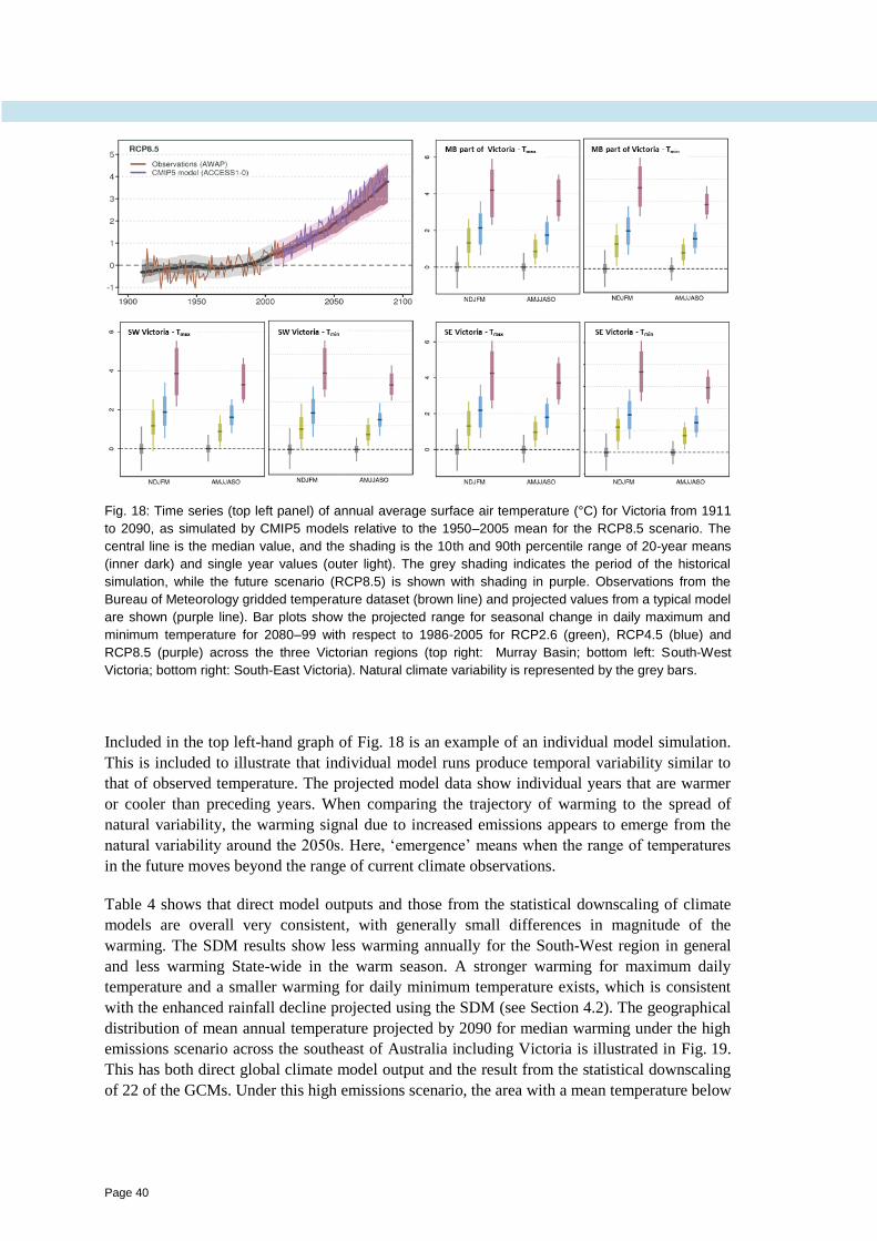
Page 40
Fig. 18: Time series (top left panel) of annual average surface air temperature (°C) for Victoria from 1911
to 2090, as simulated by CMIP5 models relative to the 1950–2005 mean for the RCP8.5 scenario. The
central line is the median value, and the shading is the 10th and 90th percentile range of 20-year means
(inner dark) and single year values (outer light). The grey shading indicates the period of the historical
simulation, while the future scenario (RCP8.5) is shown with shading in purple. Observations from the
Bureau of Meteorology gridded temperature dataset (brown line) and projected values from a typical model
are shown (purple line). Bar plots show the projected range for seasonal change in daily maximum and
minimum temperature for 2080–99 with respect to 1986-2005 for RCP2.6 (green), RCP4.5 (blue) and
RCP8.5 (purple) across the three Victorian regions (top right: Murray Basin; bottom left: South-West
Victoria; bottom right: South-East Victoria). Natural climate variability is represented by the grey bars.
Included in the top left-hand graph of Fig. 18 is an example of an individual model simulation.
This is included to illustrate that individual model runs produce temporal variability similar to
that of observed temperature. The projected model data show individual years that are warmer
or cooler than preceding years. When comparing the trajectory of warming to the spread of
natural variability, the warming signal due to increased emissions appears to emerge from the
natural variability around the 2050s. Here, ‘emergence’ means when the range of temperatures
in the future moves beyond the range of current climate observations.
Table 4 shows that direct model outputs and those from the statistical downscaling of climate
models are overall very consistent, with generally small differences in magnitude of the
warming. The SDM results show less warming annually for the South-West region in general
and less warming State-wide in the warm season. A stronger warming for maximum daily
temperature and a smaller warming for daily minimum temperature exists, which is consistent
with the enhanced rainfall decline projected using the SDM (see Section 4.2). The geographical
distribution of mean annual temperature projected by 2090 for median warming under the high
emissions scenario across the southeast of Australia including Victoria is illustrated in Fig. 19.
This has both direct global climate model output and the result from the statistical downscaling
of 22 of the GCMs. Under this high emissions scenario, the area with a mean temperature below
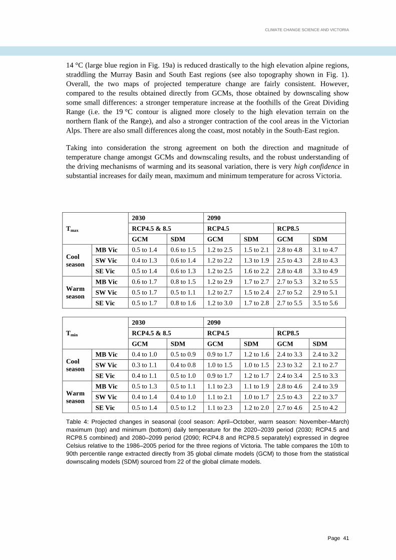
CLIMATE CHANGE SCIENCE AND VICTORIA
Page 41
14 °C (large blue region in Fig. 19a) is reduced drastically to the high elevation alpine regions,
straddling the Murray Basin and South East regions (see also topography shown in Fig. 1).
Overall, the two maps of projected temperature change are fairly consistent. However,
compared to the results obtained directly from GCMs, those obtained by downscaling show
some small differences: a stronger temperature increase at the foothills of the Great Dividing
Range (i.e. the 19 °C contour is aligned more closely to the high elevation terrain on the
northern flank of the Range), and also a stronger contraction of the cool areas in the Victorian
Alps. There are also small differences along the coast, most notably in the South-East region.
Taking into consideration the strong agreement on both the direction and magnitude of
temperature change amongst GCMs and downscaling results, and the robust understanding of
the driving mechanisms of warming and its seasonal variation, there is very high confidence in
substantial increases for daily mean, maximum and minimum temperature for across Victoria.
Tmax
2030 2090
RCP4.5 & 8.5 RCP4.5 RCP8.5
GCM SDM GCM SDM GCM SDM
Cool
season
MB Vic 0.5 to 1.4 0.6 to 1.5 1.2 to 2.5 1.5 to 2.1 2.8 to 4.8 3.1 to 4.7
SW Vic 0.4 to 1.3 0.6 to 1.4 1.2 to 2.2 1.3 to 1.9 2.5 to 4.3 2.8 to 4.3
SE Vic 0.5 to 1.4 0.6 to 1.3 1.2 to 2.5 1.6 to 2.2 2.8 to 4.8 3.3 to 4.9
Warm
season
MB Vic 0.6 to 1.7 0.8 to 1.5 1.2 to 2.9 1.7 to 2.7 2.7 to 5.3 3.2 to 5.5
SW Vic 0.5 to 1.7 0.5 to 1.1 1.2 to 2.7 1.5 to 2.4 2.7 to 5.2 2.9 to 5.1
SE Vic 0.5 to 1.7 0.8 to 1.6 1.2 to 3.0 1.7 to 2.8 2.7 to 5.5 3.5 to 5.6
Tmin
2030 2090
RCP4.5 & 8.5 RCP4.5 RCP8.5
GCM SDM GCM SDM GCM SDM
Cool
season
MB Vic 0.4 to 1.0 0.5 to 0.9 0.9 to 1.7 1.2 to 1.6 2.4 to 3.3 2.4 to 3.2
SW Vic 0.3 to 1.1 0.4 to 0.8 1.0 to 1.5 1.0 to 1.5 2.3 to 3.2 2.1 to 2.7
SE Vic 0.4 to 1.1 0.5 to 1.0 0.9 to 1.7 1.2 to 1.7 2.4 to 3.4 2.5 to 3.3
Warm
season
MB Vic 0.5 to 1.3 0.5 to 1.1 1.1 to 2.3 1.1 to 1.9 2.8 to 4.6 2.4 to 3.9
SW Vic 0.4 to 1.4 0.4 to 1.0 1.1 to 2.1 1.0 to 1.7 2.5 to 4.3 2.2 to 3.7
SE Vic 0.5 to 1.4 0.5 to 1.2 1.1 to 2.3 1.2 to 2.0 2.7 to 4.6 2.5 to 4.2
Table 4: Projected changes in seasonal (cool season: April–October, warm season: November–March)
maximum (top) and minimum (bottom) daily temperature for the 2020–2039 period (2030; RCP4.5 and
RCP8.5 combined) and 2080–2099 period (2090; RCP4.8 and RCP8.5 separately) expressed in degree
Celsius relative to the 1986–2005 period for the three regions of Victoria. The table compares the 10th to
90th percentile range extracted directly from 35 global climate models (GCM) to those from the statistical
downscaling models (SDM) sourced from 22 of the global climate models.

Page 42
Fig. 19: Annual mean surface temperature (°C), for the present (a) and for 2090 using GCM projected
warming (b) and the statistical downscaling of GCMs (c). The 15 and 20 °C contours are shown with solid
black lines; in (b) and (c) the same contours from the original climate are plotted as dotted lines. Observed
temperature values are based on the Bureau of Meteorology operational 5 km gridded monthly data from
1986 to 2005. The future case is using the median change at 2090 under the RCP8.5 scenario from all
CMIP5 models (b) and for the 22 models for which the SDM was applied (c). Results were produced on a
5 km grid and averaged over a 0.25° grid.
Changes to temperature extremes often lead to greater impacts than changes to the mean climate. To
assess these, researchers examined CMIP5 projected changes to measures such as the hottest day in
the year, the return period of hottest day in a year, warm spell duration and frost risk days. In general
it was found that measures of extremes, such as the hottest day in a year, are projected to increase in
line with the mean warming, dependent on the period considered and the emissions scenario. To
better define changes in extreme hot temperatures, several metrics can be used to quantify the
magnitude, frequency and duration of maximum/minimum values of rare events. To better
approximate future behaviour of heatwaves, relevant extremes can be thought of as ‘extended
lengths of warm spells’. This is defined as the annual count of events with at least six consecutive
days with daily temperature maxima above the 90th percentile, as measured against a baseline
climate. The GCM projections indicate a marked increase in the warm spell duration index through
the century. The baseline is near zero, as this is a rare event in summer across Victoria. There are
very large increases projected for RCP8.5 by 2090; median warming gives an increase in warm
spells of 75 days compared to 1986–2005 mean for the Murray Basin cluster, and in excess of 100
days for the Southern Slopes cluster (Fig. 20).
Changes in the frequency of surface frost are of importance to agriculture, energy and other sectors,
and to the environment. Assessing frost occurrence directly from GCM output is not reliable, in part
because of varying biases in land surface temperatures and in part due to competing influences of
temperature, mean sea level pressure and rainfall. For this report, we examined results from the 22
statistically downscaled CMIP5 models. The statistical technique has the ability to describe local
temperature with minimal bias and hence it is possible to analyse the number of days with minimum
temperatures below 2 °C as a proxy for the risk of frost occurrences. Average numbers of frost
occurrences across the greater Murray Basin cluster are projected to decrease for all months of the
annual cycle (Fig. 21) with a greater reduction by century end (2080–2099) than by 2030. It is
interesting to note that spring frosts decline less rapidly than those in autumn and winter, which
indicates that, when combined with advanced plant phenology due to generally warmer conditions,
risks associated with late frost occurrences may not necessarily decline. This is a complex area
which requires careful modelling based on individual plant phenology.
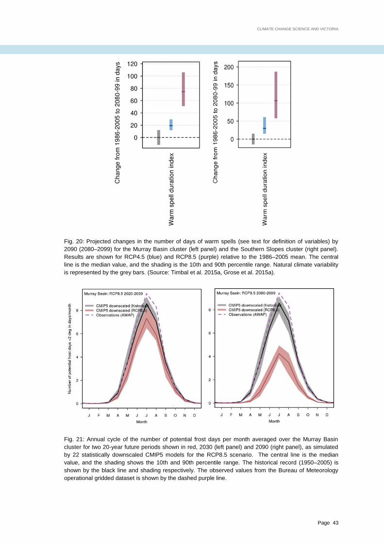
CLIMATE CHANGE SCIENCE AND VICTORIA
Page 43
Fig. 20: Projected changes in the number of days of warm spells (see text for definition of variables) by
2090 (2080–2099) for the Murray Basin cluster (left panel) and the Southern Slopes cluster (right panel).
Results are shown for RCP4.5 (blue) and RCP8.5 (purple) relative to the 1986–2005 mean. The central
line is the median value, and the shading is the 10th and 90th percentile range. Natural climate variability
is represented by the grey bars. (Source: Timbal et al. 2015a, Grose et al. 2015a).
Fig. 21: Annual cycle of the number of potential frost days per month averaged over the Murray Basin
cluster for two 20-year future periods shown in red, 2030 (left panel) and 2090 (right panel), as simulated
by 22 statistically downscaled CMIP5 models for the RCP8.5 scenario. The central line is the median
value, and the shading shows the 10th and 90th percentile range. The historical record (1950–2005) is
shown by the black line and shading respectively. The observed values from the Bureau of Meteorology
operational gridded dataset is shown by the dashed purple line.
Page 44
4.2 Rainfall and snowfall projections
In the near term (2030), there is high confidence that natural climate variability will
remain the major driver of rainfall changes from the climate of 1986–2005. Late in the
century (2090) under both RCP4.5 and RCP8.5, there is high confidence that cool
season rainfall will continue to decline and there is no clear leaning in the models
towards either wetter or drier conditions in the warm season. Apart from the simulated
direction of future changes from GCM and downscaling results, this assessment also
takes into account the physical understanding of the relationship between the
atmospheric circulation and rainfall across Victoria: specifically, how well the models
represent this relationship, and what the projected changes in the circulation are. The
understanding of physical processes coupled with high model agreement results in
high confidence that the intensity of heavy rainfall events will increase. Snowfalls are
projected to continue to decline for all RCPs with high confidence, particularly under
RCP8.5.
Annual mean rainfall projections are shown until 2090 under RCP8.5 (time series in Fig. 22) as
well as the projected percentage change averaged over 2080–2099 relative to 1986–2005 for the
warm and cool seasons for three emissions scenarios (bar plots in Fig. 22). Tabulated results for
two emission scenarios for 2030 and 2090 are given in Table 5 for both the direct GCM output
from 35 CMIP5 models and for the statistical downscaling of 22 of those models. Under any
RCP, model spread is large and the signal is not clearly separated from natural variability and
systematic biases. Model spread increases with time due to compounding uncertainty,
depending on different forcings and emission scenarios, and the models simulating more drying
events. Hence the relatively weak long-term trend in rainfall is very difficult to separate from
the effects of very large natural variability and model uncertainty, which continue during the
21st century. For the cool season, the projected drying trend is more severe and also more
robust as the magnitude of the median decline increases with the severity of the emission
scenarios (from RCP 2.6 to 8.5). In contrast, while the mean signal also indicates a rainfall
decline during the warm season, no relationship with the severity of the emission scenarios is
found, as the decline is less in the RCP8.5 pathway compared to other two mid-range scenarios,
at least for the Murray Basin and South-East regions. This non-linearity between the magnitude
of the climate forcing and the warm season rainfall response suggests that opposing
mechanisms, acting to both increase and decrease rainfall, are at play. Therefore increased
summer rainfall cannot be ruled out and several models do project an increase of warm season
rainfall.
The severity of the observed rainfall decline over the last 30 years stands out as exceptional
(Table 2). In comparison to the envelope of the climate model simulations of the 20th century
(grey shading in top left panel in Fig. 22), it represents a very extreme case, albeit one that falls
largely within the modelled range of natural variability. In comparison with the future
projections, it is on par with the most extreme modelled projections by 2090 using RCP8.5. It is
also interesting to note the similarity in the spatial pattern of the cool season rainfall decline. Of
the three Victorian regions, the Murray Basin region experienced the largest historical decline in
cool season rainfall. Declining trends are projected to be slightly larger in this region compared
to the southern regions by the end of the 21st century under all three emissions scenarios (top
right panel in Fig. 22). It is worth remembering that while climate models do reproduce the

CLIMATE CHANGE SCIENCE AND VICTORIA
Page 45
changes (MMC and STR changes, see Section 3.3 on climate model evaluation) driving the
observed cool season decline, they do so with a much reduced magnitude. Hence, it is possible
that climate models are not as sensitive as the real climate system to the overall change in
circulation impacting the region. For this reason, projected reductions in cool season rainfall
may be underestimates, and the large reductions in cool season rainfall at the extreme end of the
modelling results should not be discarded for planning purposes.
Fig. 22: Time series (top left panel) of annual average rainfall (%) for Victoria from 1900 to 2090, as
simulated by CMIP5 models relative to the 1950–2005 mean for the RCP8.5 scenario. The central line is
the median value, and the shading shows the 10th and 90th percentile range of 20-year means (inner
dark) and single year values (outer light). The grey shading indicates the period of the historical simulation,
while the future scenario (RCP8.5) is shown with purple shading. Observations from the Bureau of
Meteorology operational gridded rainfall dataset (brown) and projected values from a typical model
(purple) are shown. Bar plots show the projected range for mean rainfall (change in percentage term) for
2080–99 with respect to 1986–2005 for RCP 2.6 (green), RCP4.5 (blue) and RCP8.5 (purple) across the
three Victorian regions (top right: Murray Basin; bottom left: South-West Victoria; bottom right: South-East
Victoria) for the CMIP5 models (GCM) and for the statistical downscaling (SDM) of 22 of the CMIP5
models (only for RCP4.5 and 8.5). Natural climate variability is represented by the grey bars.
For geographical reasons, downscaling has the potential to be of benefit in further revealing
spatial details in the projected climate change signal across Victoria. Using the SDM method,
overall agreement is found with the thrust of the CMIP5 model projections (Fig. 22 and
Table 5) for the 2080–2099 periods averaged across the three regions of Victoria. Some
differences emerge due to the smaller sample of GCMs considered (22 instead of 35 GCMs for
RCP8.5). For both warm and cool seasons, the rainfall decrease is enhanced using statistical
downscaling of the GCMs. Furthermore, the consistency amongst the projections, in particular
for the cool season, is increased, although this is partly driven by the subsampling from the
CMIP5 suite of models. For example, in the case of the RCP8.5 scenario, all statistically

Page 46
downscaled models project a cool season rainfall decline in the Murray Basin region (Table 5).
This convergence amongst projections and increase of the severity of the projected drying when
the statistical downscaling method is used, is worth remembering when considering related
projections in regards to snow (later in this section) and streamflow (Section 4.5).
2030 2090
RCP4.5 & 8.5 RCP4.5 RCP8.5
GCM SDM GCM SDM GCM SDM
Annual
mean
MB Vic -14 to +4 -11 to 0 -18 to +2 -14 to -7 -31 to +8 -28 to -11
SW Vic -14 to +3 -13 to 0 -17 to +3 -15 to -5 -27 to +5 -28 to -12
SE Vic -15 to +4 -12 to +3 -18 to +3 -15 to -7 -34 to +8 -29 to -10
Cool
season
MB Vic -14 to +4 -11 to +2 -20 to +3 -14 to -5 -34 to +4 -33 to -12
SW Vic -13 to +3 -11 to +4 -15 to +4 -12 to -2 -31 to +4 -30 to -9
SE Vic -15 to +4 -12 to +4 -21 to +3 -15 to -5 -37 to +5 -35 to -12
Warm
season
MB Vic -16 to +10 -16 to +2 -23 to +2 -17 to -3 -19 to +11 -27 to -6
SW Vic -21 to +12 -20 to +1 -28 to +5 -24 to -1 -24 to +11 -33 to -18
SE Vic -17 to +11 -18 to +3 -21 to +4 -22 to -3 -18 to +11 -27 to 0
Table 5: GCM projected changes in rainfall for the 2020–2039 period (2030) and 2080–2099 period (2090)
expressed as a percentage change relative to the 1986–2005 period for the three regions of Victoria. The
table compares the 10th to 90th percentile range extracted directly from 35 global climate models (GCM) and
from the statistical downscaling of 22 of these climate models (SDM). Results are given for RCP4.5 and
RCP8.5 for the annual mean, the cool season (April to October) and the warm season (November to March).
Taking into account the physical understanding of the relationship between the mean meridional
circulation, the subtropical ridge and rainfall across Victoria (see Section 2.1) and these
projections, including the results from statistical downscaling, there is high confidence that cool
season rainfall will decline in the future. The magnitude of this decline is, however, uncertain.
In contrast, there is little confidence that future warm season rainfall will remain unchanged
across Victoria indicating that positive or negative changes are also possible. There is also high
confidence that natural variability will remain large relative to any anthropogenic changes, at
least for the near future.
The frequency of heavy rainfall events and associated flooding is projected to increase across
Victoria, despite the overall projected rainfall decline in both cool and warm seasons. In a
warming climate, heavy rainfall events are expected to increase in magnitude mainly due to a
warmer atmosphere holding more moisture (Sherwood et al. 2010). The CMIP5 models
simulate an increase in the magnitude of the annual maximum 1-day rainfall value (i.e. the
amount of rainfall that falls on the wettest day of the year) and an even greater increase in the
magnitude of the 20-year return value for maximum 1-day rainfall (where a 20-year return value
is equivalent to a 5% chance of occurrence within any one year) for the period 2080–2099
relative to the baseline period 1986–2005 (Fig. 23). The magnitudes of the changes in extreme
rainfall are strongly dependent on the emission scenario and time into the future. Comparing the
trends in the two extreme indices with that of annual mean rainfall (Fig. 23), it is evident that
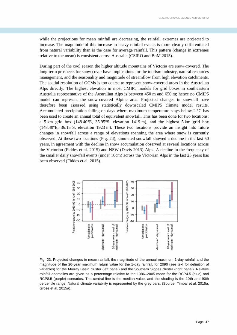
CLIMATE CHANGE SCIENCE AND VICTORIA
Page 47
while the projections for mean rainfall are decreasing, the rainfall extremes are projected to
increase. The magnitude of this increase in heavy rainfall events is more clearly differentiated
from natural variability than is the case for average rainfall. This pattern (change in extremes
relative to the mean) is consistent across Australia (CSIRO and BoM 2015).
During part of the cool season the higher altitude mountains of Victoria are snow-covered. The
long-term prospects for snow cover have implications for the tourism industry, natural resources
management, and the seasonality and magnitude of streamflow from high elevation catchments.
The spatial resolution of GCMs is too coarse to represent snow-covered areas in the Australian
Alps directly. The highest elevation in most CMIP5 models for grid boxes in southeastern
Australia representative of the Australian Alps is between 450 m and 650 m; hence no CMIP5
model can represent the snow-covered Alpine area. Projected changes in snowfall have
therefore been assessed using statistically downscaled CMIP5 climate model results.
Accumulated precipitation falling on days where maximum temperature stays below 2 °C has
been used to create an annual total of equivalent snowfall. This has been done for two locations:
a 5 km grid box (148.40°E, 35.95°S, elevation 1419 m), and the highest 5 km grid box
(148.40°E, 36.15°S, elevation 1923 m). These two locations provide an insight into future
changes in snowfall across a range of elevations spanning the area where snow is currently
observed. At these two locations (Fig. 24), simulated snowfall showed a decline in the last 50
years, in agreement with the decline in snow accumulation observed at several locations across
the Victorian (Fiddes et al. 2015) and NSW (Davis 2013) Alps. A decline in the frequency of
the smaller daily snowfall events (under 10cm) across the Victorian Alps in the last 25 years has
been observed (Fiddes et al. 2015).
Fig. 23: Projected changes in mean rainfall, the magnitude of the annual maximum 1-day rainfall and the
magnitude of the 20-year maximum return value for the 1-day rainfall, for 2090 (see text for definition of
variables) for the Murray Basin cluster (left panel) and the Southern Slopes cluster (right panel). Relative
rainfall anomalies are given as a percentage relative to the 1986–2005 mean for the RCP4.5 (blue) and
RCP8.5 (purple) scenarios. The central line is the median value, and the shading is the 10th and 90th
percentile range. Natural climate variability is represented by the grey bars. (Source: Timbal et al. 2015a,
Grose et al. 2015a).
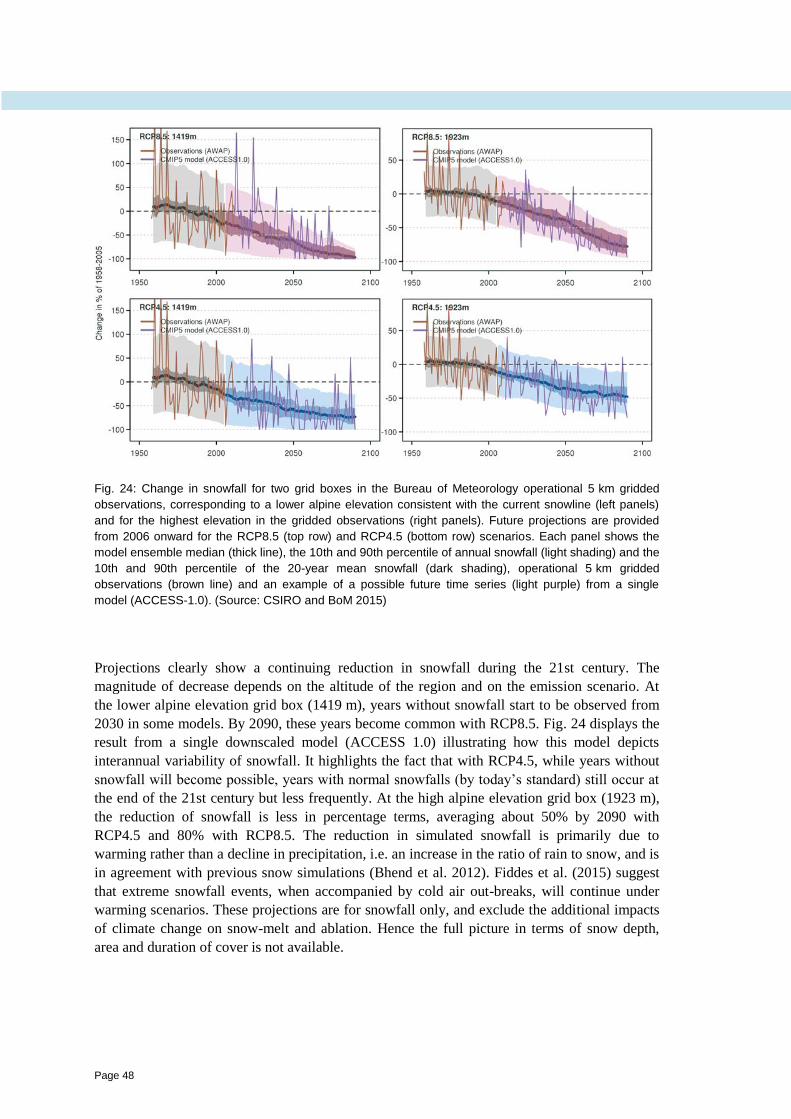
Page 48
Fig. 24: Change in snowfall for two grid boxes in the Bureau of Meteorology operational 5 km gridded
observations, corresponding to a lower alpine elevation consistent with the current snowline (left panels)
and for the highest elevation in the gridded observations (right panels). Future projections are provided
from 2006 onward for the RCP8.5 (top row) and RCP4.5 (bottom row) scenarios. Each panel shows the
model ensemble median (thick line), the 10th and 90th percentile of annual snowfall (light shading) and the
10th and 90th percentile of the 20-year mean snowfall (dark shading), operational 5 km gridded
observations (brown line) and an example of a possible future time series (light purple) from a single
model (ACCESS-1.0). (Source: CSIRO and BoM 2015)
Projections clearly show a continuing reduction in snowfall during the 21st century. The
magnitude of decrease depends on the altitude of the region and on the emission scenario. At
the lower alpine elevation grid box (1419 m), years without snowfall start to be observed from
2030 in some models. By 2090, these years become common with RCP8.5. Fig. 24 displays the
result from a single downscaled model (ACCESS 1.0) illustrating how this model depicts
interannual variability of snowfall. It highlights the fact that with RCP4.5, while years without
snowfall will become possible, years with normal snowfalls (by today’s standard) still occur at
the end of the 21st century but less frequently. At the high alpine elevation grid box (1923 m),
the reduction of snowfall is less in percentage terms, averaging about 50% by 2090 with
RCP4.5 and 80% with RCP8.5. The reduction in simulated snowfall is primarily due to
warming rather than a decline in precipitation, i.e. an increase in the ratio of rain to snow, and is
in agreement with previous snow simulations (Bhend et al. 2012). Fiddes et al. (2015) suggest
that extreme snowfall events, when accompanied by cold air out-breaks, will continue under
warming scenarios. These projections are for snowfall only, and exclude the additional impacts
of climate change on snow-melt and ablation. Hence the full picture in terms of snow depth,
area and duration of cover is not available.
CLIMATE CHANGE SCIENCE AND VICTORIA
Page 49
4.3 Mean sea level pressure and circulation changes
Rainfall changes will be driven by changes in general atmospheric circulation, in
particular a broadening of the mean meridional circulation, and accompanying changes
in mean sea level pressure (MSLP). MSLP over southern Australia is projected to
increase with high confidence, mostly during the cool season; this is driven by an
increase in the strength of the well-known belt of high pressures, the subtropical ridge,
and a shift of this ridge southward consistent with the observed trend over the last
30 years. As climate models tend to underestimate the rainfall response to changes in
the position and intensity of the subtropical ridge, these models may underestimate the
projected rainfall decline in the cool season. Other large-scale drivers (e.g. ENSO and
SAM) are also projected to change and impact future rainfall projections.
As discussed earlier, changes in mean sea level pressure (MSLP) are important as they relate to
rainfall change across Victoria, in particular during the cool season when the intensity of the
subtropical ridge (STR) has a strong influence on regional rainfall. Across southern Australia
(which includes the area where the STR is measured) annual mean MSLP is projected to
increase, reaching 1 hPa by 2090 for the RCP8.5 scenario (time series in Fig. 25). Based upon
results for the Murray Basin cluster, the projected annual mean change is made up of a small
increase during the warm season and a large increase during the cool season (bar plot in
Fig. 25). The cool season is the time of the year where the relationship between the STR
intensity and rainfall in Victoria is important. For 2090, there is high confidence in the direction
of the change, but the increase is gradual during the 21st century and its magnitude depends on
the emission scenario.
A separate analysis of the CMIP5 projections of the STR confirms that most climate models
project an increase in the intensity of the STR, depending on the magnitude of the projected
warming (Grose et al. 2015b). The STR is projected to strengthen and move poleward under
RCP8.5, a result that is highly consistent among all the climate models examined (Fig. 26).
There is a greater emphasis on an increase in intensity of the ridge rather than a shift in position
in CMIP5 (Grose et al. 2015b) compared to CMIP3 (Kent et al. 2013). An intensification of the
STR is expected to be associated with a reduction in rainfall, and is therefore consistent with the
CMIP5 model projections of a reduction of rainfall for the cool season from April to October
across Victoria (see Section 3.3). However, there is a large range in the magnitude of projected
reductions, and the poor simulation of the connection between the STR and rainfall in the
current climate suggests that the projected rainfall decline may be underestimated under
RCP8.5. A simple linear analysis using the observed relationship between STR changes and
rainfall to interpret the STR changes simulated by the climate models, suggests that the
underestimation could be around 4% in the multi-model mean but more for some single models.
The underestimation of recent trends in the intensity of the STR-I (see Section 3.3) by models
also suggests that the projected decrease in rainfall by the CMIP5 GCMs may be
underestimated. The intensification and poleward shift of the STR is consistent with the
observed trend in the last 30 years and the observed broadening of the MMC (see Section 2.1).

Page 50
Fig. 25: Time series for the Murray Basin cluster annual average MSLP (hPa), as simulated by CMIP5
models relative to the 1950–2005 mean for RCP8.5 (left). The central line is the median value, and the
shading shows the 10th and 90th percentile range of 20-year means (inner dark) and single year values
(outer light). The grey shading indicates the period of the historical simulation, while the future scenario is
shown with purple shading. HadSLP2 observations are shown in brown and projected values from a
typical model are shown into the future in purple. Bar plots (right) show seasonal changes (hPa) for
southern Australia (from Western Australia to South-Eastern Australia) for 2080–2099 with respect to
1986–2005 for RCP2.6 (green), RCP4.5 (blue) and RCP8.5 (purple). The central line is the median value,
and the shading is the 10th and 90th percentile range. Natural climate variability is represented by the grey
bars. (Source: Timbal et al. 2015a)
Fig. 26: GCM simulations of the annual cycle of STR intensity (STR-I) and position (STR-P) for the
historical period (1948–2002; light red) and for the middle (2040–2059; dark red) and end (2080–2099;
black) of the 21st century under the RCP8.5 scenario. Months are denoted by their initial letter. (Source:
Grose et al. 2015b).
CLIMATE CHANGE SCIENCE AND VICTORIA
Page 51
Grose et al. (2015b) also noted that there is a relationship between the ability of models to
reproduce the STR and rainfall projections for some areas along the Australian eastern
seaboard; this finding is relevant for the South-East region of Victoria. Models in which the
main longitudinal band of the STR is shifted west appear to generate much drier future
projections for the eastern seaboard (Grose et al. 2015b). This is worth considering when
selecting particular climate models for impact studies.
Other large-scale climate features of relevance to Victorian climate (as discussed in Section 2)
have been extensively studied. Future climate projections indicate a consensus amongst models
toward a further broadening of the MMC (IPCC 2013). The IPCC report (Chapter 12 in IPCC,
2013) also concluded that ‘there is high confidence that the El Niño-Southern Oscillation will
remain the dominant mode of year-to-year variability in the tropical Pacific, with global effects
in the 21st century. Due to the increase in moisture availability, ENSO-related precipitation
variability on regional scales will likely intensify. Natural variations of the amplitude and
spatial pattern of ENSO are large and thus confidence in any specific projected change in ENSO
and related regional phenomena for the 21st century remains low’.
Additionally, more recent work concluded that global warming will intensify El Niño-driven
drying in the western equatorial Pacific and further increase El Niño driven rainfall increases in
the central and eastern Pacific during El Niño events (Power et al. 2013, Cai et al. 2014). In the
Indian Ocean, the overall frequency of IOD events (positive and negative) is not projected to
change (Ihara et al. 2008, IPCC 2013). Changes in the Southern Annular Mode (SAM) have
exhibited a positive trend in southern summer and autumn (Marshall 2007, Jones et al. 2009a), a
change attributed to the effects of ozone depletion and the increase in greenhouse gases
(Thompson et al. 2011, IPCC 2013). While stratospheric Ozone is projected to recover,
greenhouse gas increases will be the principal driver of SAM changes into the future (assessed
as likely in chapter 14 in IPCC 2013).
4.4 Wind and weather systems
Changes in mean and extreme wind are uncertain. Mean wind is likely to decrease
during the cool season while increased occurrence of intense frontal systems with
abrupt wind ‘changes’ during the warm season are possible.
For 2030, changes in wind speed are projected with high confidence to be small under all RCPs
(± 5%) (not shown). By 2090 under RCP4.5 and RCP8.5, there is an indication in the model
results of decreased wind speed in winter (see Timbal et al. 2015a and Grose et al. 2015a for
details). This aligns with changes in atmospheric circulation already discussed and is of medium
confidence. Small or inconsistent changes are present in the other seasons. Overall, no large
changes in surface wind are expected across the State, except in winter.
Changes in extreme winds are likely to be more important for impact studies than mean wind.
Summer extreme winds occur primarily due to intense cold fronts and thunderstorms. In that
season, the interactions between frontal systems and the continent are markedly different than
during the cool season due to a stronger thermal contrast between the land and the ocean. For

Page 52
example, using a selection of CMIP3 models, Hasson et al. (2009) found that intense frontal
systems affecting southeastern Australia, associated with extreme winds and dangerous fire,
will increase strongly by end of the 21st century, although this increase is strongly affected by
the emission scenario. As these fronts tend to have the greatest impact on the western part of the
State these findings are most relevant for the South-West and Murray Basin regions. For the
South-East region changes in extreme winds are more likely to be related to any change in
ECLs. Studies in the literature suggest a continuation of the observed decreasing trend in ECLs
since the 1970s (Speer 2008), with a reduction of about 30% of ECL formation in the late 21st
century compared to the late 20th century (Dowdy et al. 2013b) based on an analysis of CMIP5
models. While the number of cut-off lows may reduce, there is some indication that their
average intensity may increase (Grose et al. 2012).
4.5 Changes in the hydrological cycle
Important changes are projected in the hydrological cycle. Linked to the rainfall
projections, there is medium confidence that the time spent in meteorological drought,
and the frequency of extreme droughts, will increase over the course of the century
under RCP8.5. Beside the changes in rainfall and temperature, changes in other
variables will also contribute to changes in the hydrological cycle. Small changes are
projected for solar radiation and relative humidity by 2030 with clear increases seen by
2090. In particular, an increase in solar radiation is linked to reduced cloud cover and
rainfall decline in conjunction with a decrease in relative humidity. Potential
evapotranspiration is projected to increase in all seasons. As a result, soil moisture and
runoff are projected to decrease with medium confidence.
One important consequence of the projected change in key climate variables (temperature,
rainfall and wind) is a follow-on effect on the frequency, duration and severity of droughts.
Drought in general means acute water shortage. The primary cause of any drought is a lack of
rainfall over an extended period of time, resulting in a water shortage for some activities,
groups, or sectors. The response of different entities (e.g. agricultural and hydrological systems)
to water shortage conditions varies substantially as a function of time scale and socio-
environmental conditions.
To assess the implications of projected climate change for drought occurrence, the Standardised
Precipitation Index (SPI) was selected as a measure of meteorological drought (McKee et al.
1993, Lloyd-Hughes and Saunders 2002). This index is based solely on rainfall. More details on
the calculation of the SPI can be found in the Technical Report for the National Climate Change
Projections (CSIRO and BoM 2015). The projected change in the percentage time spent in
drought, as well as the projections for the duration and frequency for extreme drought, are
shown in Fig. 27 for the two NRM clusters overlapping with the Victorian regions. The
proportion of time spent in any category of drought (from mild to extreme) is projected to
increase through the century, especially by 2090 under RCP8.5. This result is associated with
the projected decline in annual and cool season rainfall, although changes in rainfall variability
may contribute. The duration and frequency of droughts in the extreme category are also
projected to increase, with smaller changes in lower categories. Median projections are similar
for the two clusters north and south of the Great Dividing Range; the range of projections is
larger for the Murray Basin cluster, potentially leading to very large increases in extreme

CLIMATE CHANGE SCIENCE AND VICTORIA
Page 53
drought duration as well as possible decreases. Because the projections of meteorological
drought depend on projections of mean rainfall, the direction of any change in drought is
typically the same as that of the mean annual rainfall, although they also reflect changes in
variability. There is some indication that ENSO events, which have a strong influence on
Victorian rainfall (Section 2.2), will have an increased influence over western equatorial Pacific
Ocean under global warming (Power et al. 2013) leading to a possible intensification of El Niño
related droughts over Victoria.
Surface water availability across Victoria is affected by more than rainfall, temperature and
wind changes, discussed in Sections 4.1, 4.2 and 4.4. Changes in incoming solar radiation will
affect the energy budget and partitioning across the landscape, leading in turn to changes in
humidity at the surface, evapotranspiration and subsequently soil moisture, runoff across the
landscape and streamflow. Projecting these changes requires methodologies able to resolve
these finer scale processes.
Fig. 27: CMIP5 simulated changes in drought based on the Standardised Precipitation Index (SPI) for the
Murray Basin cluster (top panels) and the Southern Slopes cluster (bottom panels). The multi-model
ensemble results show the percentage of time in drought (i.e. for SPI less than –1) (left panels), duration of
extreme drought (middle panels) and frequency of extreme drought (right panels) for each 20-year period
centred on 1995, 2030, 2050, 2070 and 2090 under RCP2.6 (green), RCP4.5 (blue) and RCP8.5 (purple).
Natural climate variability is represented by the grey bars. See CSIRO and BoM (2015), chapter 7.2.3 for
definition of drought indices. (Source: Timbal et al. 2015a, Grose et al. 2015a).

Page 54
The CMIP5 models project small changes in radiation (in general less than 5%) for all RCPs
considered (RCP2.6, RCP4.5 and RCP8.5) to 2090 across southeast Australia (Fig. 28). The
largest projected mean change is up to 7% for the Murray Basin cluster for RCP8.5 in winter and
about half that in spring; while for the Southern Slopes cluster, the projected increase is similar for
winter and spring, at close to 5%. Winter and spring are the two seasons where most (but not all)
models tend to agree on an increase. Projected changes in summer and autumn are smaller with
models showing both increases and decreases (Fig. 28, left panels). As expected, the strongest
trend is found in the seasons where the largest rainfall decline is projected. It is worth noting that
an Australia-wide model evaluation suggested that some models are not able to adequately
reproduce the climatology of solar radiation (Moise et al. 2015). Globally, CMIP5 models appear
to underestimate the observed trends in some regions due to underestimation of aerosol direct
radiative forcing and deficient aerosol emission inventories (Allen et al. 2013). Taking this into
account, we have high confidence in increased winter and spring radiation projections by 2090.
Relative humidity depends on the absolute amount of moisture in the atmosphere and the
ambient temperature and pressure. For example, for the same absolute amount of moisture, an
atmosphere with higher temperature will have a lower relative humidity compared to a cooler
atmosphere. For this reason, without circulation changes, absolute atmospheric moisture is
expected to increase with global warming but relative humidity will decrease. Across Victoria,
the magnitudes of the projected decreases in relative humidity depend on the emission scenario
and are modulated by the direction of the rainfall projections (Fig. 28, middle panels). By 2090,
mean decreases are up to 5% in spring for the Murray Basin cluster, and close to 3% for the
Southern Slopes cluster; the mean projected decrease is larger for spring than for winter, and for
these two seasons most models agree on the direction of the change consistent with the rainfall
and radiation projections. In contrast, projected changes in summer and autumn are smaller,
with models showing both increases and decreases. In all seasons, there are, however, models
that simulate increases in relative humidity, as evident by large positive 90th percentile values.
Climate models have a reasonable ability to simulate the climatology of global humidity, and
we conclude that for winter and spring there is high confidence for substantial decrease while
for summer and autumn there is medium confidence in a small decrease.
Amongst the various possible measures of evaporation, this report uses Morton’s wet-
environmental potential evapotranspiration, which is a derived measure of potential evaporation
and transpiration demand assuming a wet environment (McMahon et al. 2013). This measure
combines inputs of air temperature, relative humidity and downward solar radiation at the
surface. Overall, the Morton method compares favourably with other methods used to calculate
potential evaporation in rainfall-runoff modelling (Chiew and McMahon 1991) and is strongly
correlated to pan evaporation observations (Kirono et al. 2009). With increasing temperatures
due to global warming and an intensified hydrological cycle, potential evapotranspiration is
generally expected to increase. For Victoria, projected seasonal changes for potential
evapotranspiration relative to the 1986–2005 baseline period are shown for the end of the 21st
century (Fig. 28, right panel). Climate models strongly agree on an increase of wet-environment
potential evapotranspiration across all seasons. The increases are similar in both clusters
(Murray Basin and Southern Slopes) with the largest increases in percentage terms for winter
(20–25%) and 10–15% in the other seasons. As potential evaporation is much larger during the
warm part of the year, in absolute terms, the largest increases in potential evaporation are found

CLIMATE CHANGE SCIENCE AND VICTORIA
Page 55
in summer and autumn, with smaller increases in winter and spring. Although there is high
confidence in an increase, there is only medium confidence in the magnitude of this change.
Fig. 28: Projected changes by 2090 in (a) solar radiation (%), (b) relative humidity (%, absolute change)
and (c) wet-environmental potential evapotranspiration (%) for the Murray Basin cluster (top panels) and
the Southern Slopes cluster (bottom panels). The bar plots show seasonal projections with respect to the
1986–2005 mean for RCP2.6 (green), RCP4.5 (blue) and RCP8.5 (purple). Natural climate variability is
represented by the grey bars. (Source: Timbal et al. 2015a, Grose et al. 2015a).
As a consequence of the changes in surface temperature and rainfall projected across Victoria, the
land surface partitioning of energy and moisture is projected to change as was described for solar
radiation, humidity and evapotranspiration across Victoria. In turn a reduction in soil moisture,
runoff and streamflow is expected. However, soil moisture, runoff and streamflow are difficult to
simulate. This is particularly true in climate models where, due to their relatively coarse
resolution, the models cannot simulate much of the rainfall detail that is important to many
hydrological processes. For these reasons, additional tools were used to provide these projections.

Page 56
As a first estimate, hydrological models were forced by CMIP5 simulated rainfall and potential
evapotranspiration to derive a soil moisture estimate based on an extension of the Budyko
framework (Zhang et al. 2008) as a part of the NRM reports. The projected seasonal soil
moisture changes across Victoria for 2090 are summarised in Fig. 29 (left panels) for the
Murray Basin (top panels) and the Southern Slopes (lower panels) NRM clusters. Decreases
dominate, particularly in winter and spring and are largest for RCP8.5. The annual mean
changes for the high emission scenario range from around −1 to –10%. The largest declines are
projected for the Murray Basin cluster in winter and spring. In summer and autumn where the
mean decline is smaller, larger values are projected for the Southern Slopes cluster compared to
the Murray Basin cluster. Consistent with the directly simulated surface moisture, the
percentage changes in soil moisture are strongly influenced by those in rainfall, but tend to be
more negative due to the increase in potential evapotranspiration.
Fig. 29: Projected change in seasonal soil moisture (left) and annual runoff (right) (Budyko method—see
text) for the Murray Basin cluster (top panels) and the Southern Slopes cluster (bottom panels). Anomalies
are given for 2080–2099 in percentage term with respect to the 1986–2005 mean for RCP4.5 (blue) and
RCP8.5 (purple). Natural climate variability is represented by the grey bars. (Source: Timbal et al. 2015a,
Grose et al. 2015a).

CLIMATE CHANGE SCIENCE AND VICTORIA
Page 57
Runoff was also derived from the long-term annual water and energy balance using the Budyko
framework (Teng et al. 2012) and is presented as change in 20-year averages. Projected runoff
is inferred from 30-year means of rainfall and potential evapotranspiration for each CMIP5
model for which data are available. The median and ranges for the Murray Basin cluster in the
final 20-year period are shown in the right panels of Fig. 29. The median change for 2090 under
RCP8.5 is a decrease of about 20% for the southern part of the State and slightly more for the
Murray Basin, with the majority of models giving a decrease in both regions; it is noteworthy
that these estimates have a very large uncertainty range. Despite the high confidence about the
mean rainfall decline during the cool season, there is only low confidence in these projections.
This arises because the method used is not able to consider changes to rainfall intensity,
seasonality and changes in vegetation characteristics, which are all factors that could impact
future runoff. More detailed runoff and streamflow projections for Victoria are being prepared
as part of the Victorian Climate Initiative and will be reported separately.
4.6 Change in bushfire risk
There is high confidence that climate change will result in a harsher fire-weather
climate regime in the future. However, there is only low confidence in the magnitude of
the projected change to fire weather, as this depends on rainfall projections and their
seasonal variation. The summer rainfall increase projected by some climate models, if
it eventuates, would moderate the number of severe fire-weather days, although there
is very little confidence about this projection.
Change in bushfire risk is assessed using three CMIP5 models, chosen to provide a wide spread
of results across Victoria. Using a method similar to that of Hennessy et al. (2005), monthly-
mean changes to maximum temperature, rainfall, relative humidity and wind speed from these
models are applied to observation-based high-quality historical fire-weather records (Lucas
2010). A period centred on 1995 (i.e. 1981–2010, the last 30 years of existing observations
when that study was completed) serves as the baseline. These records are modified using the
changes from the three models for two 30-year time slices (centred on 2030 and 2090) and the
RCP4.5 and RCP8.5 emission scenarios; more details on the methodology used are provided in
CSIRO and BoM (2015). In Victoria, significant fire activity occurs primarily in areas
characterised by forests and woodlands; fuel is abundant and the ‘weather switch’, well-
characterized by FFDI, is key to fire occurrence (see Section 1.3 for details).
Five stations are used to describe the spatial changes of fire risk across Victoria: Mt Gambier (in
South Australia but close to the western border of the State), Mildura, Laverton, Melbourne
Airport and East Sale (all are shown in Fig. 1); and an average of these five stations is provided.
It should be noted that, as large parts of the State—including all the Alpine regions—are not
covered, it should not be regarded as a State average. Focusing on the 2030 and 2090 time
slices, the results indicate increased fire-weather risk in the future (Table 6). Across the State,
the sum of all daily FFDI values over a year is broadly indicative of general fire-weather risk.
This index increases by about 10% by 2030, about 15% under RCP4.5 by 2090, and 35% under
RCP8.5 by 2090. The number of days with a ‘severe’ fire danger rating increases by about 30%
by 2030, and by 30–60% with RCP4.5 to 85–185% with RCP8.5 by 2090.
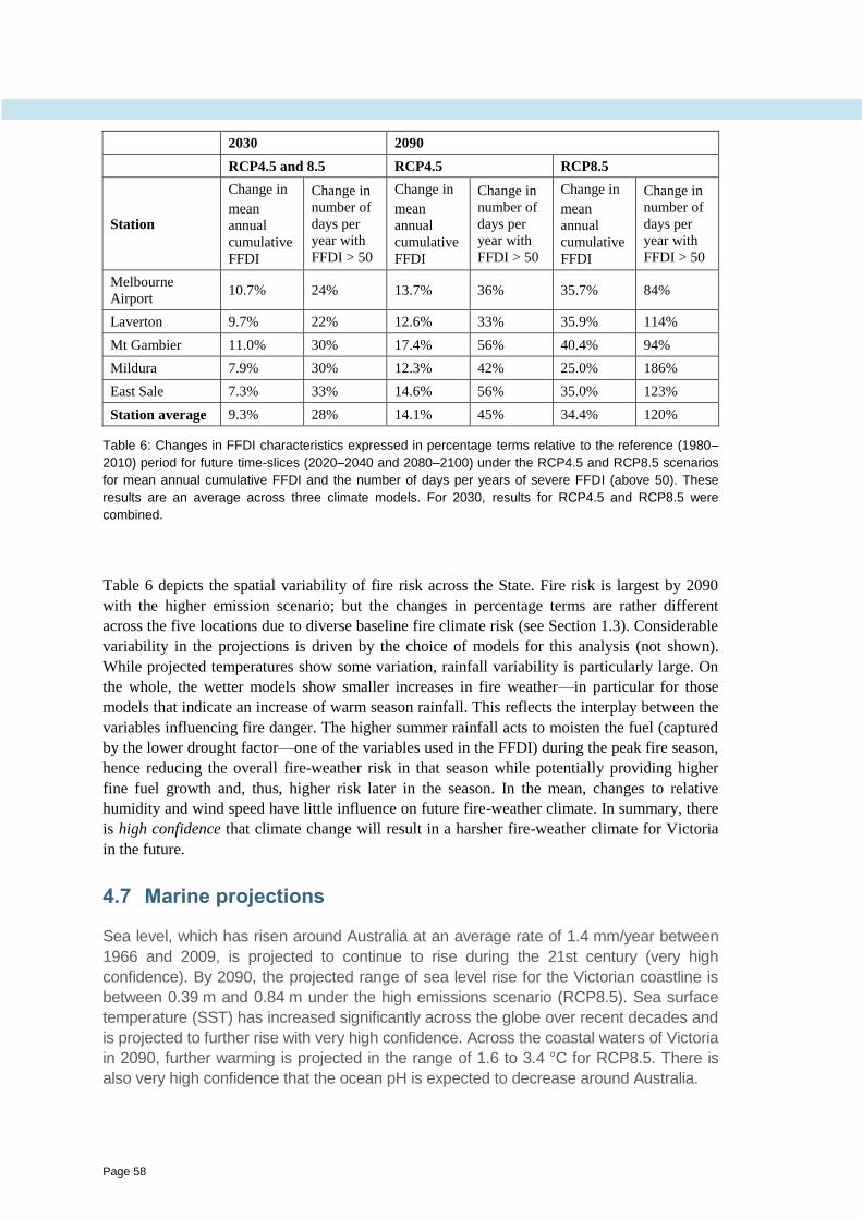
Page 58
2030 2090
RCP4.5 and 8.5 RCP4.5 RCP8.5
Station
Change in
mean
annual
cumulative
FFDI
Change in
number of
days per
year with
FFDI > 50
Change in
mean
annual
cumulative
FFDI
Change in
number of
days per
year with
FFDI > 50
Change in
mean
annual
cumulative
FFDI
Change in
number of
days per
year with
FFDI > 50
Melbourne
Airport 10.7% 24% 13.7% 36% 35.7% 84%
Laverton 9.7% 22% 12.6% 33% 35.9% 114%
Mt Gambier 11.0% 30% 17.4% 56% 40.4% 94%
Mildura 7.9% 30% 12.3% 42% 25.0% 186%
East Sale 7.3% 33% 14.6% 56% 35.0% 123%
Station average 9.3% 28% 14.1% 45% 34.4% 120%
Table 6: Changes in FFDI characteristics expressed in percentage terms relative to the reference (1980–
2010) period for future time-slices (2020–2040 and 2080–2100) under the RCP4.5 and RCP8.5 scenarios
for mean annual cumulative FFDI and the number of days per years of severe FFDI (above 50). These
results are an average across three climate models. For 2030, results for RCP4.5 and RCP8.5 were
combined.
Table 6 depicts the spatial variability of fire risk across the State. Fire risk is largest by 2090
with the higher emission scenario; but the changes in percentage terms are rather different
across the five locations due to diverse baseline fire climate risk (see Section 1.3). Considerable
variability in the projections is driven by the choice of models for this analysis (not shown).
While projected temperatures show some variation, rainfall variability is particularly large. On
the whole, the wetter models show smaller increases in fire weather—in particular for those
models that indicate an increase of warm season rainfall. This reflects the interplay between the
variables influencing fire danger. The higher summer rainfall acts to moisten the fuel (captured
by the lower drought factor—one of the variables used in the FFDI) during the peak fire season,
hence reducing the overall fire-weather risk in that season while potentially providing higher
fine fuel growth and, thus, higher risk later in the season. In the mean, changes to relative
humidity and wind speed have little influence on future fire-weather climate. In summary, there
is high confidence that climate change will result in a harsher fire-weather climate for Victoria
in the future.
4.7 Marine projections
Sea level, which has risen around Australia at an average rate of 1.4 mm/year between
1966 and 2009, is projected to continue to rise during the 21st century (very high
confidence). By 2090, the projected range of sea level rise for the Victorian coastline is
between 0.39 m and 0.84 m under the high emissions scenario (RCP8.5). Sea surface
temperature (SST) has increased significantly across the globe over recent decades and
is projected to further rise with very high confidence. Across the coastal waters of Victoria
in 2090, further warming is projected in the range of 1.6 to 3.4 °C for RCP8.5. There is
also very high confidence that the ocean pH is expected to decrease around Australia.
CLIMATE CHANGE SCIENCE AND VICTORIA
Page 59
Changes in sea levels and their extremes, as well as sea surface temperatures and ocean pH
(acidity) have the potential to impact both the coastal terrestrial and marine environments. This
is discussed at length in chapter 8 of the Technical Report for the National Climate Change
Projections (CSIRO and BoM 2015). Of particular significance for the terrestrial environment
of coastal Victoria is the impact of sea level rise and changes to the frequency of extreme sea
levels. Impacts will be felt through coastal flooding and erosion. For the adjacent marine
environment, increases in ocean temperatures and acidity may alter the distribution and
composition of marine ecosystems and impact vegetation and coastal fisheries.
Changes in sea level are caused primarily by changes in ocean density (e.g. ‘thermal
expansion’) and changes in ocean mass due to the exchange of water with the terrestrial
environment, including from glaciers and ice sheets. Sea levels have risen around the Australian
coastline at an average rate of 2.1 mm/year over 1966–2009; including an accelerated rise of
3.1 mm/year over 1993–2009. Projections of future sea level changes are shown for Stony Point
in Victoria (Fig. 30). The rate of sea level rise during the 21st century will be larger than the
average rate during the 20th century as radiative forcing from greenhouse gas emissions
continues to grow (Fig. 30). For the first decades of the 21st century the projections are almost
independent of the emission scenario. The rate of rise continues to increase through the 21st
century and for the RCP8.5 scenario the sea level ends up being about 30% higher than with the
RCP4.5 level by 2100. Significant interannual variability will continue through the 21st century
as indicated by the dotted lines in Fig. 30. These ranges of sea level rise are considered likely (at
least 66% probability); however, if a collapse in the marine based sectors of the Antarctic ice
sheet were initiated, these projections could be several tenths of a metre higher by late in the
century (IPCC 2013). Continued increases in sea level for this location and coastal Victoria in
general are projected with very high confidence.
In addition to mean sea level rise, impact studies need to consider that extreme coastal sea
levels are exacerbated by rising sea levels and are caused by a combination of factors including
astronomical tides, storm surges and wind-waves. Along the south coast of Victoria, the
majority of storm surges occur in conjunction with the passage of cold fronts during the winter
months (e.g. McInnes and Hubbert 2003). Using the method of Hunter (2012), it is possible to
compute an allowance based on the mean sea level rise, uncertainty around the rise, and taking
into account the nature of extreme sea levels along the Victorian coastline. The Technical
Report for the National Climate Change Projections (CSIRO and BoM 2015) provides details
on the approach and the cluster report for the Southern Slopes (Grose et al. 2015a) illustrates the
application for Victorian coastal areas.
Sea surface temperatures (SSTs) have increased significantly across the globe over recent
decades (IPCC 2013). Increases in SSTs pose a significant threat to the marine environment
through biological changes in marine species, including local abundance and community
structure. For the Victorian coastline, the range of projected SST increases from Portland in
western Bass Strait to eastern Bass Strait. It also increases with time and according to the
emission scenario considered. For example, in Portland, the SST warming is projected to be 0.3
to 0.8 °C by 2030 with RCP8.5, rising to 1.6 to 3.4 °C by 2090. There is very high confidence
that sea surface temperatures will continue to rise along the Victorian coastline, with the
magnitude of the warming dependent on emission scenarios.

Page 60
Fig. 30: Observed and projected relative sea level change (metre) relative to 1993–2010 for Stony Point,
Victoria. The observed tide gauge sea level records are indicated in black, with the satellite record (since
1993) shown in mustard and the tide gauge reconstruction (which has lower variability) shown in blue.
Multi-model mean projections are shown for the RCP8.5 and RCP2.6 scenarios (thick purple and olive
lines) as well as RCP4.5 and RCP6.0, with uncertainty ranges shown by the purple and olive shaded
regions from 2006–2100. The mustard and blue dashed lines are estimates of inter-annual variability in
sea level (i.e. likely uncertainty range for the projections) and indicate that individual monthly averages of
sea level can be above or below longer term averages. Note that the ranges of sea level rise should be
considered likely (at least 66% probability) and that if a collapse in the marine based sectors of the
Antarctic ice sheet were initiated, these projections could be several tenths of a metre higher by late in the
century. (Source: Grose et al. 2015a).
Ocean salinity in coastal waters will be affected by changes to rainfall and evaporation and may
impact on upwelling and mixing, and potentially nutrient supply. Changes to salinity across the
coastal waters of Victoria can also be affected by riverine input. As changes in salinity are
related to changes in the hydrological cycle, they are of low confidence.
About 30% of the anthropogenic carbon dioxide emitted into the atmosphere over the past 200
years has been absorbed by the oceans (Ciais et al. 2013). As carbon dioxide enters the ocean it
reacts with the seawater to cause a decrease in pH and carbonate concentration, collectively
known as ocean acidification. Ocean acidification can affect fin and shellfish fisheries,
aquaculture, tourism and coastal protection. Along Victorian coastlines, by 2030 pH change is

CLIMATE CHANGE SCIENCE AND VICTORIA
Page 61
projected to be another 0.08 units lower relative to 1986-2005; by 2090 this is projected to be up
to 0.3 units lower for RCP8.5. These changes together with SST changes will affect all levels of
the marine food web, and make it harder for calcifying marine organisms to build their hard
shells, potentially affecting the resilience and viability of marine ecosystems. There is very high
confidence that the ocean will become more acidic, and that the rate of ocean acidification will
be proportional to carbon dioxide emissions.

Page 62
5. FURTHER INFORMATION
The climate change projections presented in this report are the most comprehensive and broadly
based ever produced for the State of Victoria, complementing the report recently released as
part of the national climate change projections. They also incorporate state-of-the-art
understanding of the complexity of the climate system in this part of the world. These
projections provide an excellent basis for impact and adaptation activities.
This has been made possible by advances in modelling and in observations, and also by the
research of scientists working over the past decade on many aspects of southeastern Australia
climate and associated processes, as part of both the South Eastern Australia Climate Initiative
(SEACI) from 2006 to 2012, and the Victorian Climate Initiative (VicCI) since 2013. These
regional science programs were established to inform water resource planning and management
through improved prediction and understanding of the climate system and its representation by
climate models, and to improve understanding of the linkages between climate and water
availability. This strategic knowledge provides the basis for improved projections of future
climate and associated water availability; in particular, it enhances knowledge of the
uncertainties in future projections.
For a regional climate science program such as VicCI it is vital to be in regular communication
with related programs at the national and international level. The present report is a clear
example, being rooted in the development of national climate change projections delivered in
2015 (CSIRO and BoM, 2015, supported over the years by the Australian Climate Change
Science Program (ACCSP), and further supported by phase 5 of the Coupled Model
Intercomparison Project (CMIP5) and an increase in international scientific understanding of
the global climate system, as presented in the recent reports of the IPCC (IPCC 2013).
A particular aim of VicCI is to encourage the hydrology and climate research communities to
collaborate, leading to more comprehensive research outcomes. Climate is clearly the main
driver of hydrology, and in turn, the needs of the hydrological community can influence the
research focus of the climate community. The nexus between climatology and hydrology
provides opportunities for meaningful discussion between research disciplines, leading to better
informed water resource planning and management.

CLIMATE CHANGE SCIENCE AND VICTORIA
Page 63
REFERENCES
Alexander, L., Wang, X., Wan, H. and Trewin, B. 2011. Significant decline in storminess over
southeast Australia since the late 19th century. Australian Meteorological and. Oceanographic
Journal, 61, 23–30.
Allan, R. and Ansell, T. 2006. A new globally complete monthly historical gridded mean sea
level pressure dataset (HadSLP2): 1850–2004. Journal of Climate, 19, 5816–5842.
Allen, R. J., Norris, J. R. and Wild, M. 2013. Evaluation of multidecadal variability in CMIP5
surface solar radiation and inferred underestimation of aerosol direct effects over Europe,
China, Japan, and India. Journal of Geophysical Research-Atmospheres, 118, 6311–6336.
Beard, G., Chandler, E., Watkins, A. and Jones, D. 2011. How does the 2010–11 La Niña
compare with past La Niña events. Bulletin of the Australian Meteorological and
Oceanographic Society, 24, 17–20.
Berry, G., Reeder, M. and Jakob, C. 2011. A global climatology of atmospheric fronts.
Geophysical Research Letters, 38. L04809
Bhend J., Bathols J. and Hennessy K. 2012. Climate change impacts on snow in Victoria.
CAWCR Report. Retrieved from:
http://www.climatechange.vic.gov.au/data/assets/pdf_file/0005/200795/
cawcr_report_on_climate change_and_Victorian_snow_final-dec12_web.pdf
Bhend, J. and Whetton, P. 2015. Evaluation of simulated recent climate change in Australia,
Australian Meteorological and. Oceanographic Journal, 65, 4–18.
Bradstock, R. 2010. A biogeographic model of fire regimes in Australia: current and future
implications. Global Ecology and Biogeography, 19, 145–158.
Bureau of Meteorology, 2012. Australia’s wettest two-year period on record: 2020–11. Special
Climate Statement No. 38, National Climate Centre, Bureau of Meteorology.
Cai, W., Borlace, S., Lengaigne, M., Van Rensch, P., Collins, M., Vecchi, G., Timmermann, A.,
Santoso, A., McPhaden, M., Wu, L., England, M., Wang, G., Guilyardi, E. and Jin, F. 2014.
Increasing frequency of extreme El Niño events due to greenhouse warming. Nature Climate
Change, 4, 111–116.
Cai, W., Van Rensch, P., Cowan, T. and Hendon, H. H. 2011. Teleconnection pathways of
ENSO and the IOD and the mechanisms for impacts on Australian rainfall. Journal of
Climate, 24(15), 3910–3923.
Chiew, F. and McMahon, T. 1991. The Applicability of Morton’s and Penman’s
Evapotranspiration Estimates in Rainfall-Runoff Modeling. Journal of the American Water
Resources Association, 27, 611–620.

Page 64
Ciais, P., Sabine, C., Bala, G., Bopp, L., Brovkin, V., Canadell, J., Chhabra, A., Defries, R.,
Galloway, J., Heimann, M., Jones, C., Le Quéré, C., Myneni, R. B., Piao, S. and Thornton, P.
2013. Carbon and Other Biogeochemical Cycles. Contribution of Working Group I to the Fifth
Assessment Report of the Intergovernmental Panel on Climate Change. In: Stocker, T. F., D.
Qin, G.- K. Plattner, M. Tignor, S.K. Allen, J. Boschung, A. Nauels, Y. Xia, Bex, V. and
Midgley, P. M. (eds.) Climate Change 2013: The Physical Science Basis. Cambridge, United
Kingdom and New York, NY, USA: Cambridge University Press.
CSIRO. 2010. Climate Variability and Change in South-Eastern Australia: A Synthesis of
Findings from Phase 1 of the South Eastern Australian Climate Initiative (SEACI). Retrieved
from http://www.seaci.org/publications/documents/SEACI-1eports/Phase1_SynthesisReport.pdf
CSIRO. 2012. Climate and water availability in southeastern Australia: A synthesis of findings
from Phase 2 of the South Eastern Australian Climate Initiative (SEACI), 41. Retrieved from
http://www.seaci.org/publications/documents/SEACI2Reports/SEACI_Phase2_Synthesis
Report.pdf
CSIRO and Bureau of Meteorology. 2015. Climate Change in Australia Information for
Australia's Natural Resource Management Regions: Technical Report. CSIRO and Bureau of
Meteorology, Australia, 222 pp. Retrieved from http://www.climatechangeinaustralia.gov.au/
Davis, C. 2013. Towards the development of long term winter records for the Snowy
Mountains. Australian Meteorological and Oceanographic Journal, 63(2), 303–313.
Dee, D. et al. 2011. The ERA-Interim reanalysis: Configuration and performance of the data
assimilation system. Quarterly Journal of the Royal Meteorological Society, 137(656), 553–
597.
Department of the Environment. 2013. Natural resource management (Online). Commonwealth
of Australia: http://www.environment.gov.au/land/nrs/science/ibra
Dittus, A., Karoly, D., Lewis, S. and Alexander, L. 2015. An investigation of some unexpected
frost day increases in southern Australia, Australian Meteorological and Oceanographic
Journal, 64(4), 261–271.
Dowdy, A., Mills, G. and Timbal, B. 2013a. Large-scale diagnostics of extratropical
cyclogenesis in eastern Australia. International Journal of Climatology, 33(10), 2318–2327.
Dowdy, A., Mills, G., Timbal, B. and Wang, Y. 2013b. Changes in the Risk of Extratropical
Cyclones in Eastern Australia. Journal of Climate, 26(4), 1403–1417.
Drosdowsky, W. 2005. The latitude of the subtropical ridge over eastern Australia: The L index
revisited. International Journal of Climatology, 25(10), 1291–1299.
Ekström M., Grose M. and Whetton, P. 2015. An appraisal of downscaling methods used in
climate change research. WIRES Climate Change, 6(3), 301–319.

CLIMATE CHANGE SCIENCE AND VICTORIA
Page 65
England, M., Ummenhofer, C. and Santoso, A. 2006. Interannual rainfall extremes over
southwest Western Australia linked to Indian ocean climate variability. Journal of Climate, 19,
1948–1969.
Fawcett, R., Trewin, B., Braganza, K, Smalley, R., Jovanovic, B. and Jones, D.A. 2012. On the
sensitivity of Australian temperature trends and variability to analysis methods and observation
networks. CAWCR Technical Report No. 50, Bureau of Meteorology, Melbourne, 66 pp.
Fiddes, S., Pezza, A. and Barras, V. (2015). A new perspective on Australian snow.
Atmospheric Science Letters, 16(3), 246–252.
Fiddes, S. and Timbal, B. 2016a. Assessment and reconstruction of catchment streamflow
trends and variability in response to rainfall across Victoria, Australia. Climate Research,
Accepted article: DOI: 10.3354/cr01355
Fiddes, S. and Timbal, B. 2016b. Future impacts of climate change on streamflows across
Victoria, Australia: making use of statistical downscaling. Submitted to Climate Research.
Frederiksen, J., Frederiksen, C., Osbrough, S. and Sisson, J. Changes in Southern Hemisphere
rainfall, circulation and weather systems. 19th International Congress on Modelling and
Simulation, 2011 Perth, Australia. Modelling and Simulation Society of Australia and New
Zealand, 2712–2718.
Gallant, A., Karoly, D. and Gleason, K. 2014. Consistent Trends in a Modified Climate
Extremes Index in the United States, Europe, and Australia. Journal of Climate, 27, 1379–1394.
Grose, M., Pook, M., McIntosh, P., Risbey, J. and Bindoff, N. 2012. The simulation of cutoff
lows in a regional climate model: reliability and future trends. Climate Dynamics, 39, 445–459.
Grose, M. et al. 2015a. Southern Slopes Cluster Report, Climate Change in Australia
Projections for Australia’s Natural Resource Management Regions: Cluster Reports, eds.
Ekström, M. et al. CSIRO and Bureau of Meteorology, Australia.
Grose, M., Timbal, B., Wilson, L., Bathols, J. and Kent, D. 2015b. The subtropical ridge in
CMIP5 models, and implications for projections of rainfall in southeast Australia. Australian
Meteorology and Oceanography Journal, 65, 90–106.
Grose, M., Risbey, J., Black, M. and Karoly, D. 2015c. Attribution of Exceptional Mean Sea
Level Pressure Anomalies South of Australia in August 2014. Bulletin of the American
Meteorological Society, 96(12), S158–S162.
Guilyardi, E., Wittenberg, A., Fedorov, A., Collins, M., Wang, C., Capotondi, A. and Stockdale,
T. 2009. Understanding El Niño in ocean-atmosphere general circulation models: Progress and
challenges. Bulletin American Meteorological Society, 90, 325–340.
Hasson, A., Mills, G., Timbal, B. and Walsh, K. 2009. Assessing the impact of climate change
on extreme fire-weather events over southeastern Australia. Climate Research, 39, 159–172.
Page 66
Hendon, H., Lim, E., Arblaster, J. and Anderson, D. 2014. Causes and predictability of the
record wet east Australian spring 2010. Climate Dynamics, 42, 1155–1174.
Hendon, H., Thompson, D. and Wheeler, M. 2007. Australian Rainfall and Surface Temperature
Variations Associated with the Southern Hemisphere Annular Mode. Journal of Climate,
20(11), 2452–2467.
Hennessy, K., Lucas, C., Nicholls, N., Bathols, J., Suppiah, R. and Ricketts, J. 2005. Climate
change impacts on fire weather in southeast Australia. Melbourne, Australia: Consultancy
report for the New South Wales Greenhouse Office, Victorian Department of Sustainability and
Environment, Tasmanian Department of Primary Industries, Water and Environment, and the
Australian Greenhouse Office. CSIRO Atmospheric Research and Australian Government
Bureau of Meteorology, 78 pp. Retrieved from http:// laptop.deh.gov.au/soe/
2006/publications/drs/pubs/334/lnd/ld_24_climate_change_impacts_on_fire_weather.pdf
Hope, P., Grose, M., Timbal, B., Dowdy, A., Bhend, J., Katzfey, J., Bedin, T. and Whetton, P.
2015a. Seasonal and regional signature of the projected southern Australia rainfall reduction,
Australian Meteorological and. Oceanographic Journal, 65, 54–71.
Hope, P., Timbal, B., Hendon, H., Ekström, M., Moran, R., Manton, M., Lucas, C., Nguyen, H.,
Lim, E-P., Luo, J-J., Liu, G., Zhao, M., Fiddes S., Kirono, D., Wilson, L., Potter, N. and Teng,
J. 2015. Victorian Climate Initiative: Annual Report 2014–15, Bureau Research Report No. 5,
Bureau of Meteorology, Melbourne, 128 pp.
Hunter, J. 2012. A simple technique for estimating an allowance for uncertain sea-level rise.
Climatic Change, 113, 239–252.
Ihara, C., Kushnir, Y. and Cane, M. 2008. Warming trend of the Indian Ocean SST and Indian
Ocean dipole from 1880 to 2004. Journal of Climate, 21, 2035–2046.
IPCC. 2001. Climate change 2001: the scientific basis. In: Houghton, J. T., Ding, Y., Griggs, D.
J., Noguer, M., Van der Linden, P. J., Dai, X., Maskell, K. and Johnson, C. (eds.). Cambridge:
Cambridge University Press .
IPCC. 2007. Climate change 2007—the physical science basis: Working group I contribution to
the fourth assessment report of the IPCC. In: Solomon, S. (ed.). Cambridge: Cambridge
University Press.
IPCC. 2013. Climate Change 2013: The Physical Science Basis. Contribution of Working
Group I to the Fifth Assessment Report of the Intergovernmental Panel on Climate Change. In:
Stocker, TF., Qin D. Plattner G.-K., Tignor M., Allen SK., Boschung J., Nauels A., Xia Y., Bex
V. and Midgley PM. (ed.). IPCC, Geneva, Switzerland.
Jakob, D. 2010. Challenges in developing a high-quality surface wind-speed dataset for
Australia. Australian Meteorological Magazine, 60, 227–236.
Jones, J., Fogt, R., Widmann, M., Marshall, G., Jones, P. and Visbeck, M. 2009a. Historical
SAM Variability. Part I: Century-Length Seasonal Reconstructions. Journal of Climate, 22,
5319–5345.
CLIMATE CHANGE SCIENCE AND VICTORIA
Page 67
Jones, D. A., Wang, W. and Fawcett, R. 2009b. High quality spatial climate datasets for
Australia. Australian Meteorological and. Oceanographic Journal, 58, 233–248.
Kalnay, E., Kanamitsu, M., Kistler, R., Collins, W., Deaven, D., Derber, J., Gandin, L., Iredell,
M., Saha, S., White, G., Woollen, J., Zhu, Y., Chelliah, M., Ebisuzaki, W., Higgins, W.,
Janowiak, J., Mo, K., Ropelewski, C., Wang, J., Leetma, A., Reynolds, R., Jenne, R. and
Joseph, D. 1996. The NCEP/NCAR 40-year reanalysis project. Bulletin of the American
Meteorological Society, 77, 437–471.
Kent, D., Kirono, D., Timbal, B. and Chiew, F. 2013. Representation of the Australian sub‐
tropical ridge in the CMIP3 models. International Journal of Climatology, 33, 48–57.
Kirono, D., Jones, R. and Cleugh, H. 2009. Pan-evaporation measurements and Morton-point
potential evaporation estimates in Australia: are their trends the same? International Journal of
Climatology, 29, 711–718.
Leblanc, M., Tweed, S., Van Dijk, A. and Timbal, B. 2012. A review of historic and future
hydrological changes in the Murray–Darling Basin. Global and Planetary Change, 80–81, 226–
246.
Lim, E.-P. and Hendon, H. 2015a. Understanding and predicting the strong Southern Annular
Mode and its impact on the record wet east Australian spring 2010. Climate Dynamics, 44,
2807–2824.
Lim, E.-P. and Hendon, H. 2015b. Understanding the contrast of Australian springtime rainfall
of 1997 and 2002 in the frame of two flavors of El Niño. Journal of Climate, 28, 2804–2822,
Lim, E.-P., Hendon, H. and Zhao, M. 2016. Inter-decadal variations in the linkages between
ENSO, the IOD and south-eastern Australian springtime rainfall in the past 30 years. Submitted
to Climate Dynamics.
Lloyd-Hughes, B. and Saunders, M. A. 2002. A drought climatology for Europe. International
Journal of Climatology, 22, 1571–1592,
Lucas, C. 2010. On developing a historical fire weather dataset for Australia. Australian
Meteorological Magazine, 60, 1–13.
Lucas, C., Nguyen, H. and Timbal, B. 2012. An observational analysis of Southern Hemisphere
tropical expansion. Journal of Geophysical Research-Atmospheres, 117.
Lucas, C., Timbal, B. and Nguyen, H. 2014. The expanding tropics: a critical assessment of the
observational and modeling studies. Climate Change, 5, 89–112.
Marshall, G. 2003. Trends in the Southern Annular Mode from observations and reanalyses.
Journal of Climate, 16(24), 4134–4143.
Marshall, G. 2007. Half-century seasonal relationships between the Southern Annular Mode and
Antarctic temperatures. International Journal of Climatology, 27, 1549–1555.

Page 68
McArthur, A. 1967. Fire behaviour in Eucalypt forests. Leaflet. Forestry Timber Bureau
Australia, 35–35.
McBride, J. and Nicholls, N. 1983. Seasonal relationships between Australian rainfall and the
Southern Oscillation. Monthly Weather Review, 111, 1998–2004.
McGregor, J. and Dix, M. 2008. An updated description of the conformal-cubic atmospheric
model. High resolution numerical modelling of the atmosphere and ocean, Springer: 51–76.
McInnes, K. and Hubbert, G. 2003. A numerical modelling study of storm surges in Bass Strait.
Australian Meteorological Magazine, 52, 143–156.
McKee, T., Doesken, N. and Kleist, J. 1993. The relationship of drought frequency and duration
to time scales. Proceedings of the 8th Conference on Applied Climatology, American
Meteorological Society Boston, MA, 179–183.
McMahon, T., Peel, M., Lowe, L., Srikanthan, R. and McVicar, T. 2013. Estimating actual,
potential, reference crop and pan evaporation using standard meteorological data: a pragmatic
synthesis. Hydrology and Earth System Sciences, 17, 1331–1363.
McVicar, T., Roderick, M., Donohue, R., Li, L., Van Niel, T., Thomas, A., Grieser, J.,
Jhajharia, D., Himri, Y. and Mahowald, N. 2012. Global review and synthesis of trends in
observed terrestrial near-surface wind speeds: Implications for evaporation. Journal of
Hydrology, 416, 182–205.
Meyers, G., McIntosh, P., Pigot, L. and Pook, M. 2007. The Years of El Niño, La Niña, and
Interactions with the Tropical Indian Ocean. Journal of Climate, 20(13), 2872–2880.
DOI:10.1175/JCLI4152.1
Mills, G. A. 2005. A Re-examination of the Synoptic Mesoscale Meteorology of Ash
Wednesday 1983, Australian Meteorological Magazine, 54, 35–55.
Murphy, B., Timbal, B., Hendon, H., Ekström, M., Moran, R., Manton, M., Lucas, C., Nguyen,
H., Rikus, L., Lim, E-P., Liu, G., Zhao, M., Fiddes S., Grosse, M., Bathols, J., Kirono D. and
Teng, J. 2014. Victorian Climate Initiative: Annual Report 2013–14, CAWCR Technical Report
No. 76, Bureau of Meteorology, Melbourne, 154 pp.
Moise, A., Wilson, L., Grose, M., Whetton, P., Watterson, I., Bhend, J., Bathols, J., Hanson, L.,
Erwin, T., Bedin, T., Heady, C. and Rafter, T. 2015. Evaluation of CMIP3 and CMIP5 models
over the Australian region to inform confidence in projections, Australian Meteorological and.
Oceanographic Journal, 65, 19–53
Morice, C., Kennedy, J., Rayner, N. and Jones, P. 2012. Quantifying uncertainties in global and
regional temperature change using an ensemble of observational estimates: The HadCRUT4
dataset. Journal of Geophysical Research: Atmospheres (1984–2012), 117.
Nakićenović, N. and Swart, R. (eds.) 2000. Special Report on Emissions Scenarios. A Special
Report of Working Group III of the Intergovernmental Panel on Climate Change, Cambridge,
United Kingdom and New York, NY, USA: Cambridge University Press.

CLIMATE CHANGE SCIENCE AND VICTORIA
Page 69
Nguyen, H., Evans, A., Lucas, C., Smith, I., and Timbal, B. 2013. The Hadley Circulation in
Reanalyses: Climatology, Variability, and Change. Journal of Climate, 26(10), 3357–3376.
Nguyen H., Lucas, C. Evans, A., Timbal B. and Hanson, L. 2015. Expansion of the Southern
Hemisphere Hadley Cell in response to greenhouse gas forcing. Journal of Climate, 28, 8067–
8077
Pepler, A., Timbal, B., Rakich, C. and Coutts-Smith, A. 2014. Indian Ocean Dipole Overrides
ENSO’s Influence on Cool Season Rainfall across the Eastern Seaboard of Australia. Journal of
Climate, 27(10), 3816–3826.
Pook, M. J., Risbey, J. S. and McIntosh, P. C. 2012. The synoptic climatology of cool-season
rainfall in the Central Wheatbelt of Western Australia. Monthly Weather Review, 140, 28–43
Power, S. and Colman, R. 2006. Multi-year predictability in a coupled general circulation
model. Climate Dynamics, 26, 247-272.
Power, S., Delage, F., Chung, C., Kociuba, G. and Keay, K. 2013. Robust twenty-first-century
projections of El Niño and related precipitation variability. Nature, 502, 541–545.
Power, S., Tseitkin, F., Torok, S., Lavery, B., Dahni, R. and McAvaney, B. 1998. Australian
temperature, Australian rainfall and the Southern Oscillation, 1910-1992: coherent variability
and recent changes. Australian Meteorological Magazine, 47(2), 85–101.
Rayner, N.A., P. Brohan, D.E. Parker, C.K. Folland, J.J. Kennedy, M. Vanicek, T. Ansell and
S.F.B. Tett, 2006: Improved analyses of changes and uncertainties in sea surface temperature
measured in situ since the mid-nineteenth century: the HadSST2 dataset. J. Climate. 19(3) 446–
469
Risbey, J., Pook, M., McIntosh, P., Ummenhofer, C. and Meyers, G. 2009a. Characteristics and
variability of synoptic features associated with cool season rainfall in southeastern Australia.
International Journal of Climatology, 29, 1595–1613.
Risbey, J. S., Pook, M. J., McIntosh, P. C., Wheeler, M. C. and Hendon, H. H. 2009b. On the
Remote Drivers of Rainfall Variability in Australia. Monthly Weather Review, 137(10), 3233–
3253.
Saji, N. H., Goswami, B. N., Viayachandran, P. N. and Yamagata, T. 1999. A dipole mode in
the tropical Indian Ocean. Nature, 401, 360–363.
Sherwood, S. C., Roca, R., Weckwerth, T. M. and Andronova, N. G. 2010. Tropospheric water
vapor, convection, and climate. Reviews of Geophysics, 48, RG2001.
Simmonds, I. and Keay, K. 2000. Mean southern hemisphere extratropical cyclone behavior in
the 40-year NCEP-NCAR reanalysis. Journal of Climate, 13(5), 873–885.
Simmonds, I., Keay, K. and Bye, J. 2012. Identification and Climatology of Southern
Hemisphere Mobile Fronts in a Modern Reanalysis. Journal of Climate, 25, 1945–1962.
Page 70
Sinclair Knight Merz. 2010. Developing guidelines for the selection of streamflow gauging
stations. Malvern, Victoria, Australia: Sinclair Knight Merz Pty Ltd. Retrieved from:
http://www.bom.gov.au/water/hrs/papers/SKM2010_Report.pdf
Speer, M. S. 2008. On the late twentieth century decrease in Australian east coast rainfall
extremes. Atmospheric Science Letters, 9, 160–170.
Sturman, A. P. and Tapper, N. J. 2006. The weather and climate of Australia and New Zealand.
2nd edition. Oxford University Press: South Melbourne.
Taylor, K., Stouffer, R. and Meehl, G. 2012. An overview of CMIP5 and the experiment design.
Bulletin of the American Meteorological Society, 93, 485–498.
Teng, J., Chiew, F., Vaze, J., Marvanek, S. and Kirono, D. 2012. Estimation of climate change
impact on mean annual runoff across continental Australia using Budyko and Fu equations and
hydrological models. Journal of Hydrometeorology, 13, 1094–1106.
Thompson, D., Solomon, S., Kushner, P., England, M., Grise, K. and Karoly, D. 2011.
Signatures of the Antarctic ozone hole in Southern Hemisphere surface climate change. Nature
Geoscience, 4, 741–749.
Thompson, D. and Wallace, J. 2000. Annular modes in the extratropical circulation. Part I:
Month-to-month variability. Journal of Climate, 13, 1000–1016.
Timbal, B. and Drosdowsky, W. 2013. The relationship between the decline of Southeastern
Australian rainfall and the strengthening of the subtropical ridge. International Journal of
Climatology, 33(4), 1021–1034.
Timbal, B., Fernandez E. and Z. Li. 2009. Generalization of a statistical downscaling model to
provide local climate change projections for Australia. Environmental Modelling and Software,
24, 341–358
Timbal, B. and Hendon, H. 2011. The role of tropical modes of variability in the current rainfall
deficit across the Murray-Darling basin. Water Resources Research, 47(12), W00G09
Timbal, B. et al. 2015a. Murray Basin Cluster Report, Climate Change in Australia Projections
for Australia’s Natural Resource Management Regions: Cluster Reports, eds. Ekström, M. et al.
CSIRO and Bureau of Meteorology, Australia
Timbal, B., Griffiths, M. and Tan, K. 2015b. Rainfall and streamflows in the Greater Melbourne
catchment area: variability and recent anomalies. Climate Research, 63(3), 215–232.
Trewin, B. 2013. A daily homogenized temperature dataset for Australia. International Journal
of Climatology, 33, 1510–1529.
Troccoli, A., Muller, K., Coppin, P., Davy, R., Russell, C. and Hirsch, A. 2012. Long-term wind
speed trends over Australia. Journal of Climate, 25, 170–183.
CLIMATE CHANGE SCIENCE AND VICTORIA
Page 71
Turner, M., Bari, M., Amirthanathan, G. and Z. Ahmad. 2012. Australian network of hydrologic
reference stations - advances in design, development and implementation. Proceedings of
Hydrology and Water Resources Symposium, 1555–1564. 2012.
Van Vuuren, D., Edmonds, J., Kainuma, M., Riahi, K., Thomson, A., Hibbard, K., Hurtt, G. C.,
Kram, T., Krey, V. and Lamarque, J.-F. 2011. The representative concentration pathways: an
overview. Climatic Change, 109, 5–31.
Watterson, I. 1996. Nondimensional measures of climate model performance, International
Journal of Climatology, 16, 379–391
Watterson, I., Hirst, A. and Rotstayn, L. 2013. A skill score based evaluation of simulated
Australian climate. Australian Meteorological and Oceanographic Journal, 63, 181–190.
Whetton, P., Hennessy, K., Clarke, J., McInnes, K. and Kent, D. 2012. Use of Representative
Climate Futures in impact and adaptation assessment. Climatic Change, 115, 433–442.
Zhang, L., Potter, N., Hickel, K., Zhang, Y. and Shao, Q. 2008. Water balance modeling over
variable time scales based on the Budyko framework – Model development and testing. Journal
of Hydrology, 360, 117–131.

Page 72
APPENDICES
Appendix 1: Observational datasets
Several datasets are used to describe the observed climate of Victoria, its variability and long-
term trends and to evaluate its representation in model simulations.
For assessment of rainfall and temperature across Victoria, the observed data are derived from
the Australian Water Availability Project (AWAP) (Jones et al. 2009b). This is the current
operational gridded dataset used by the Bureau of Meteorology and the data are accessible on-
line. The highest resolution available for these gridded observations is a regular grid of 0.05° in
latitude and longitude which approximates to a regular grid of 5 by 5 km.
Some global datasets are relied upon to derive global quantities and large-scale indices:
Surface temperatures are from HadCRUT4, a 5 by 5 degree gridded dataset (Morice et al.
2012), used as a measure of observed global warming;
Sea Surface Temperatures (SST) are from HadISST, a 1 by 1 degree gridded dataset
(Rayner et al. 2006), from which SST indices such as those depicting ENSO variability
(Niño 3, 3.4 and 4 indices), Indian Ocean variability (IOD) and the tripole index (Timbal
and Hendon 2011), are computed; and
Mean sea level pressures (MSLP) are from HadSLP2, a 5 by 5 degree gridded dataset
(Allan and Ansell 2006), used to derive regional measures of MSLP.
Additional regional or local datasets relied upon are:
Fire-weather data, based on Bureau of Meteorology local observations of surface
parameters combined into a fire-weather index (Lucas 2010);
Local subtropical ridge (STR) intensity and position, computed both from Bureau of
Meteorology local observations of MSLP and from reanalysis data using the method of
Drosdowsky (2005);
The Southern Annular Mode (SAM) index, derived from observed MSLP in locations
across the Southern Hemisphere mid-latitudes (Marshall 2003); and
Streamflow data, derived from the Hydrologic Reference Station (HRS) network compiled
by the Bureau of Meteorology (Turner et al. 2012).
Quantities for which observations are lacking are obtained from reanalysis datasets for the
current climate. These datasets are derived using a systematic approach whereby all available
observations over a historical period are used in a consistent manner to produce a ‘complete’
climate record. This unchanging analysis framework provides a dynamically consistent estimate
of the climate state at each time step. Reanalysis datasets are typically used for climate
monitoring purposes. Two main reanalysis datasets are relied upon in this report:
The 2.5 by 2.5 degree reanalyses prepared jointly by the National Center for Environmental
Prediction (NCEP) and the National Center for Atmospheric Research (NCAR), labelled
NNR in the report (Kalnay et al. 1996); and

CLIMATE CHANGE SCIENCE AND VICTORIA
Page 73
The 0.75 by 0.75 degree interim reanalyses prepared by the European Centre for Medium-
range Weather Forecast (ECMWF), labelled ERA-I in the report (Dee et al. 2011).
Appendix 2: Understanding projection plots
Projections based on climate model results are illustrated using time series (a) and bar plots (b).
The model data are expressed as anomalies from a reference climate. For the time series (a),
anomalies are calculated as relative to 1950–2005, and for the bar plots (b) anomalies are
calculated as the change between 1986–2005 and 2080–2099 (referred to elsewhere as ‘2090’).
The time series plots used a different reference period to the bar plots due to technical reasons
in producing visually representative time series plots where simulations of the historical and
future time periods are merged into a long series. The graphs can be summarised as follows:
1. The middle (bold) line in both (a) and (b) is the median value of the model simulations (20-
year moving average); half the model results fall above and half below this line.
2. The thick bars in (b) and dark shaded areas in (a) show the range (10th to 90th percentile) of
model simulations of 20-year average climate.
3. Line segments in (b) and light shaded areas in (a) represent the projected range (10th to
90th percentile) of individual years taking into account year-to-year variability in addition
to the long-term response (20-year moving average).
In the time series (a), where available, an observed time series (4) is overlaid to enable
comparison between observed variability and simulated model spread. A time series of the
future climate from one model is shown to illustrate what a possible future may look like (5).
ACCESS1-0 was used for RCP4.5 and 8.5, and BCC-CSM-1 was used for RCP2.6, as
ACCESS1-0 output was not available. In both (a) and (b), different RCPs are shown in different
colours (6). Throughout this document, green is used for RCP2.6, blue for RCP4.5 and purple
for RCP8.5, with grey bars used in bar plots (b) to illustrate the expected range of change due to
natural internal climate variability alone (7).
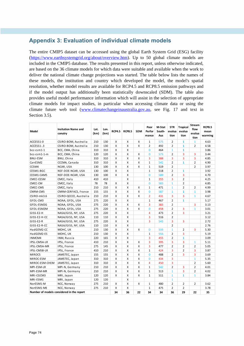
Page 74
Appendix 3: Evaluation of individual climate models
The entire CMIP5 dataset can be accessed using the global Earth System Grid (ESG) facility
(https://www.earthsystemgrid.org/about/overview.htm). Up to 50 global climate models are
included in the CMIP5 database. The results presented in this report, unless otherwise indicated,
are based on the 36 climate models for which data were suitable and available when the work to
deliver the national climate change projections was started. The table below lists the names of
these models, the institution and country which developed the model, the model's spatial
resolution, whether model results are available for RCP4.5 and RCP8.5 emission pathways and
if the model output has additionally been statistically downscaled (SDM). The table also
provides useful model performance information which will assist in the selection of appropriate
climate models for impact studies, in particular when accessing climate data or using the
climate future web tool (www.climatechangeinaustralia.gov.au, see Fig. 17 and text in
Section 3.5).
ModelInsitution Name and
conutry
Lat.
(km)
Lon.
(km)RCP4.5 RCP8.5 SDM
Poor
Perfor
mance
M-Stat
South-
Aus
STR
evalua
tion
Tropical
evalua
tion
Stream
flow
evalua
tion
RCP8.5
mean
warming
ACCESS1-0 CSIRO-BOM, Austra l ia 210 130 X X X 1 575 2 1 1 4.63
ACCESS1-.3 CSIRO-BOM, Austra l ia 210 130 X X X 2 492 2 1 2 4.58
bcc-csm1-1 BCC, CMA, China 310 310 X X 0 464 1 1 3.86
bcc-csm1-1-m BCC, CMA, China 120 120 X X X 0 573 2 3 3 3.44
BNU-ESM BNU, China 310 310 X X X 3 388 3 3 3 4.85
CanESM2 CCCMA, Canada 310 310 X X X 1 542 2 1 2 4.90
CCSM4 NCAR, USA 130 100 X X X 1 519 2 2 3.97
CESM1-BGC NSF-DOE-NCAR, USA 130 100 X X 1 518 2 1 3.92
CESM1-CAM5 NSF-DOE-NCAR, USA 130 100 X X 0 589 2 3 4.70
CMCC-CESM CMCC, Ita ly 410 410 X 1 355 3 2 4.25
CMCC-CM CMCC, Ita ly 78 78 X X 0 583 1 2 4.85
CMCC-CMS CMCC, Ita ly 210 210 X X X 1 471 1 2 2 4.99
CNRM-CM5 CNRM-CERFACS, France 155 155 X X X 0 587 1 1 1 3.98
CSIRO-mk3.6 CSIRO-QCCCE, Austra l ia 210 210 X X X 2 431 3 3 1 4.67
GFDL-CM3 NOAA, GFDL, USA 275 220 X X 1 467 2 1 5.17
GFDL-ESM2G NOAA, GFDL, USA 275 220 X X X 3 383 2 3 3.13
GFDL-ESM2M NOAA, GFDL, USA 275 220 X X X 0 458 2 3 1 3.01
GISS-E2-H NASA/GISS, NY, USA 275 220 X X 4 473 2 3 3.21
GISS-E2-H-CC NASA/GISS, NY, USA 110 110 X X 3 516 2 3.12
GISS-E2-R NASA/GISS, NY, USA 275 220 X X 3 543 3 3 2.72
GISS-E2-R-CC NASA/GISS, NY, USA 110 110 X X 2 2.76
HadGEM2-CC MOHC, UK 210 130 X X X 0 533 1 2 3 5.30
HadGEM2-ES MOHC, UK 210 130 X X 1 556 2 3 5.19
INMCM4 INM, Russ ia 220 165 X X 3 455 2 1 3.09
IPSL-CM5A-LR IPSL, France 410 210 X X X 3 395 3 3 1 5.11
IPSL-CM5A-MR IPSL, France 275 145 X X X 3 477 2 2 2 5.05
IPSL-CM5B-LR IPSL, France 410 210 X X X 1 424 3 2 3 3.87
MIROC5 JAMSTEC, Japan 155 155 X X X 0 488 2 3 3 3.69
MIROC-ESM JAMSTEC, Japan 310 310 X X X 0 434 3 1 5.35
MIROC-ESM-CHEM JAMSTEC, Japan 310 310 X X X 4 450 3 2 5.60
MPI-ESM-LR MPI-N, Germany 210 210 X X X 1 542 2 3 2 4.01
MPI-ESM-MR MPI-N, Germany 210 210 X X X 1 513 1 3 2 4.02
MRI-CGCM3 MRI, Japan 120 120 X X X 1 511 1 1 1 3.84
MRI-ESM1 MRI, Japan 120 120 X 1
NorESM1-M NCC, Norway 275 210 X X X 1 480 2 2 2 3.62
NorESM1-ME NCC, Norway 275 210 X X 1 475 2 2 3.78
34 36 22 34 34 36 29 22 35Number of models considered in the report

CLIMATE CHANGE SCIENCE AND VICTORIA
Page 75
The metrics applied to evaluate the models listed in the table are:
‘Poor performance’ was evaluated in the Technical Report for the National Climate Change
Projections (table 5.6.1, p. 76 in CSIRO and BoM, 2015), as the number of times a model
scored low (6 to 8 lowest score) on various skill metrics used in that report; here 0 score is
indicated in blue and 3+ in red.
The ‘M-statistic’ (Watterson 1996) was computed for temperature, rainfall and MSLP for
each climate model across the southern part of the Australian continent (reported in table
5.2.2, p. 60 in CSIRO and BoM, 2015). Higher numbers indicate more skilful models; here
a score below 460 is indicated in red and above 530 in blue (the mean is 490).
The ‘STR evaluation’ reflects the ability of each model to reproduce the observed
subtropical ridge (Grose et al. 2015b). Climate models that simulate the subtropical ridge in
the correct longitude band are scored as 1 (blue), climate models that simulate the
longitudinal band of STR as too wide or shifted are scored as 3 (red), all other models for
which a slightly larger longitude band had to be used compare to the observations are
scored as 2 (black).
The ‘tropical evaluation’ evaluates the ability of the climate models to capture tropical
variability in relation to rainfall across southeastern Australia. This assessment was
conducted using three metrics: the variability and trends of tropical SSTs and their
relationship, on interannual timescales, with rainfall in the region. The models which were
always ranked as average or better are given a 1 (blue), the models which were always
ranked as average or below are given a 3 (red), all other models are scored as 2 (black),
indicating mixed results.
The ‘streamflow evaluation’ reflects the ability of statistically downscaled models to
reproduce the observed streamflow, via a simple linear relationship. This was assessed
(Fiddes and Timbal 2016b) on the mean and variance of the reconstructed streamflow; the
seven models with the best score are indicated by a 1 (blue) and the models with the 6
poorest performances are scored as a 3 (red), all other models are scored as 2 (black).
Not all climate models used in this report were evaluated for all statistics; in this case no score
is reported. For each column the total numbers of models considered is indicated.
The final column in the table is the global sensitivity of the model measured by the mean global
warming obtained in response to the RCP8.5 pathway by the end of the 21st century (2081–
2100).
As some models stand out as performing worse on several metrics, and others, in contrast, are
consistently performing better, the information provided in this Appendix needs to be
considered when accessing climate change projections from the Climate Change in Australia
website alongside the information provided with the Climate Future tool
(www.climatechangeinaustralia.gov.au).
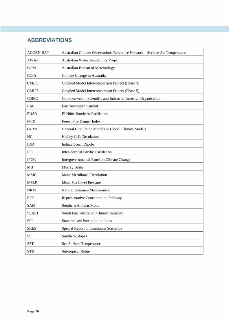
Page 76
ABBREVIATIONS
ACORN-SAT Australian Climate Observations Reference Network – Surface Air Temperature
AWAP Australian Water Availability Project
BOM Australian Bureau of Meteorology
CCIA Climate Change in Australia
CMIP3 Coupled Model Intercomparison Project (Phase 3)
CMIP5 Coupled Model Intercomparison Project (Phase 5)
CSIRO Commonwealth Scientific and Industrial Research Organisation
EAC East Australian Current
ENSO El Niño–Southern Oscillation
FFDI Forest Fire Danger Index
GCMs General Circulation Models or Global Climate Models
HC Hadley Cell/Circulation
IOD Indian Ocean Dipole
IPO Inter-decadal Pacific Oscillation
IPCC Intergovernmental Panel on Climate Change
MB Murray Basin
MMC Mean Meridional Circulation
MSLP Mean Sea Level Pressure
NRM Natural Resource Management
RCP Representative Concentration Pathway
SAM Southern Annular Mode
SEACI South East Australian Climate Initiative
SPI Standardised Precipitation Index
SRES Special Report on Emissions Scenarios
SS Southern Slopes
SST Sea Surface Temperature
STR Subtropical Ridge

CLIMATE CHANGE SCIENCE AND VICTORIA
Page 77
GLOSSARY OF TERMS
Adaptation The process of adjustment to actual or expected climate and its effects Adaptation
can be autonomous or planned.
Incremental adaptation
Adaptation actions where the central aim is to maintain the essence and integrity of
a system or process at a given scale.
Transformational adaptation
Adaptation that changes the fundamental attributes of a system in response to
climate and its effects.
Atmosphere The gaseous envelope surrounding the Earth. The dry atmosphere consists almost
entirely of nitrogen and oxygen, together with a number of trace gases (e.g. argon,
helium) and greenhouse gases (e.g. carbon dioxide, methane, nitrous oxide). The
atmosphere also contains aerosols and clouds.
Carbon dioxide A naturally occurring gas, also a by-product of burning fossil fuels from fossil
carbon deposits, such as oil, gas and coal, of burning biomass, of land use changes
and of industrial processes (e.g. cement production). It is the principal
anthropogenic greenhouse gas that affects the Earth’s radiative balance.
Climate The average weather experienced at a site or region over a period of many years,
ranging from months to many thousands of years. The relevant measured
quantities are most often surface variables such as temperature, rainfall and wind.
Climate change A change in the state of the climate that can be identified (e.g. by statistical tests)
by changes in the mean and/or variability of its properties, and that persists for an
extended period of time, typically decades or longer.
Climate projection A climate projection is the simulated response of the climate system to a
scenario of future emission or concentration of greenhouse gases and aerosols
generally derived using climate models. Climate projections are distinguished
from climate predictions by their dependence on the
emission/concentration/radiative forcing scenario used, which in turn is based on
assumptions concerning, for example, future socioeconomic and technological
developments that may or may not be realised.
Climate scenario A plausible and often simplified representation of the future climate, based on an
internally consistent set of climatological relationships that has been constructed
for explicit use in investigating the potential consequences of anthropogenic
climate change, often serving as input to impact models.
Climate sensitivity The effective climate sensitivity (in °C) is an estimate of the global mean surface
temperature response to doubled carbon dioxide concentration that is evaluated
from model output or observations for evolving non-equilibrium conditions.
Climate variability Climate variability refers to variations in the mean state and other statistics (such
as standard deviations, the occurrence of extremes, etc.) of the climate on all
spatial and temporal scales beyond that of individual weather events. Variability
may be due to natural internal processes within the climate system (internal
variability), or to variations in natural or anthropogenic external forcing (external
variability).
CMIP3 and CMIP5 Phases three and five of the Coupled Model Intercomparison Project (CMIP3 and
CMIP5), which coordinated and archived climate model simulations based on
shared model inputs by modelling groups from around the world. The CMIP3
multi-model dataset includes projections using SRES emission scenarios. The
CMIP5 dataset includes projections using the Representative Concentration
Pathways.
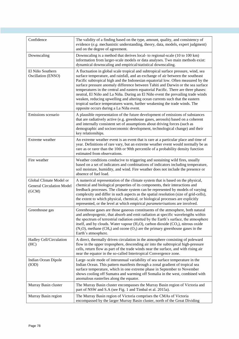
Page 78
Confidence The validity of a finding based on the type, amount, quality, and consistency of
evidence (e.g. mechanistic understanding, theory, data, models, expert judgment)
and on the degree of agreement.
Downscaling Downscaling is a method that derives local- to regional-scale (10 to 100 km)
information from larger-scale models or data analyses. Two main methods exist:
dynamical downscaling and empirical/statistical downscaling.
El Niño Southern
Oscillation (ENSO)
A fluctuation in global scale tropical and subtropical surface pressure, wind, sea
surface temperature, and rainfall, and an exchange of air between the southeast
Pacific subtropical high and the Indonesian equatorial low. Often measured by the
surface pressure anomaly difference between Tahiti and Darwin or the sea surface
temperatures in the central and eastern equatorial Pacific. There are three phases:
neutral, El Niño and La Niña. During an El Niño event the prevailing trade winds
weaken, reducing upwelling and altering ocean currents such that the eastern
tropical surface temperatures warm, further weakening the trade winds. The
opposite occurs during a La Niña event.
Emissions scenario A plausible representation of the future development of emissions of substances
that are radiatively active (e.g. greenhouse gases, aerosols) based on a coherent
and internally consistent set of assumptions about driving forces (such as
demographic and socioeconomic development, technological change) and their
key relationships.
Extreme weather An extreme weather event is an event that is rare at a particular place and time of
year. Definitions of rare vary, but an extreme weather event would normally be as
rare as or rarer than the 10th or 90th percentile of a probability density function
estimated from observations.
Fire weather Weather conditions conducive to triggering and sustaining wild fires, usually
based on a set of indicators and combinations of indicators including temperature,
soil moisture, humidity, and wind. Fire weather does not include the presence or
absence of fuel load.
Global Climate Model or
General Circulation Model
(GCM)
A numerical representation of the climate system that is based on the physical,
chemical and biological properties of its components, their interactions and
feedback processes. The climate system can be represented by models of varying
complexity and differ in such aspects as the spatial resolution (size of grid-cells),
the extent to which physical, chemical, or biological processes are explicitly
represented, or the level at which empirical parameterisations are involved.
Greenhouse gas
Greenhouse gases are those gaseous constituents of the atmosphere, both natural
and anthropogenic, that absorb and emit radiation at specific wavelengths within
the spectrum of terrestrial radiation emitted by the Earth’s surface, the atmosphere
itself, and by clouds. Water vapour (H2O), carbon dioxide (CO2), nitrous oxide
(N2O), methane (CH4) and ozone (O3) are the primary greenhouse gases in the
Earth’s atmosphere.
Hadley Cell/Circulation
(HC)
A direct, thermally driven circulation in the atmosphere consisting of poleward
flow in the upper troposphere, descending air into the subtropical high-pressure
cells, return flow as part of the trade winds near the surface, and with rising air
near the equator in the so-called Intertropical Convergence zone.
Indian Ocean Dipole
(IOD)
Large–scale mode of interannual variability of sea surface temperature in the
Indian Ocean. This pattern manifests through a zonal gradient of tropical sea
surface temperature, which in one extreme phase in September to November
shows cooling off Sumatra and warming off Somalia in the west, combined with
anomalous easterlies along the equator.
Murray Basin cluster The Murray Basin cluster encompasses the Murray Basin region of Victoria and
part of NSW and S.A (see Fig. 1 and Timbal et al. 2015a).
Murray Basin region The Murray Basin region of Victoria comprises the CMAs of Victoria
encompassed by the larger Murray Basin cluster, north of the Great Dividing
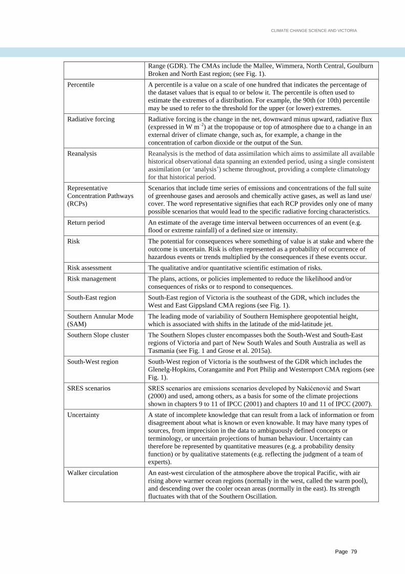
CLIMATE CHANGE SCIENCE AND VICTORIA
Page 79
Range (GDR). The CMAs include the Mallee, Wimmera, North Central, Goulburn
Broken and North East region; (see Fig. 1).
Percentile A percentile is a value on a scale of one hundred that indicates the percentage of
the dataset values that is equal to or below it. The percentile is often used to
estimate the extremes of a distribution. For example, the 90th (or 10th) percentile
may be used to refer to the threshold for the upper (or lower) extremes.
Radiative forcing Radiative forcing is the change in the net, downward minus upward, radiative flux
(expressed in W m–2
) at the tropopause or top of atmosphere due to a change in an
external driver of climate change, such as, for example, a change in the
concentration of carbon dioxide or the output of the Sun.
Reanalysis Reanalysis is the method of data assimilation which aims to assimilate all available
historical observational data spanning an extended period, using a single consistent
assimilation (or ‘analysis’) scheme throughout, providing a complete climatology
for that historical period.
Representative
Concentration Pathways
(RCPs)
Scenarios that include time series of emissions and concentrations of the full suite
of greenhouse gases and aerosols and chemically active gases, as well as land use/
cover. The word representative signifies that each RCP provides only one of many
possible scenarios that would lead to the specific radiative forcing characteristics.
Return period An estimate of the average time interval between occurrences of an event (e.g.
flood or extreme rainfall) of a defined size or intensity.
Risk The potential for consequences where something of value is at stake and where the
outcome is uncertain. Risk is often represented as a probability of occurrence of
hazardous events or trends multiplied by the consequences if these events occur.
Risk assessment The qualitative and/or quantitative scientific estimation of risks.
Risk management The plans, actions, or policies implemented to reduce the likelihood and/or
consequences of risks or to respond to consequences.
South-East region South-East region of Victoria is the southeast of the GDR, which includes the
West and East Gippsland CMA regions (see Fig. 1).
Southern Annular Mode
(SAM)
The leading mode of variability of Southern Hemisphere geopotential height,
which is associated with shifts in the latitude of the mid-latitude jet.
Southern Slope cluster The Southern Slopes cluster encompasses both the South-West and South-East
regions of Victoria and part of New South Wales and South Australia as well as
Tasmania (see Fig. 1 and Grose et al. 2015a).
South-West region South-West region of Victoria is the southwest of the GDR which includes the
Glenelg-Hopkins, Corangamite and Port Philip and Westernport CMA regions (see
Fig. 1).
SRES scenarios SRES scenarios are emissions scenarios developed by Nakićenović and Swart
(2000) and used, among others, as a basis for some of the climate projections
shown in chapters 9 to 11 of IPCC (2001) and chapters 10 and 11 of IPCC (2007).
Uncertainty A state of incomplete knowledge that can result from a lack of information or from
disagreement about what is known or even knowable. It may have many types of
sources, from imprecision in the data to ambiguously defined concepts or
terminology, or uncertain projections of human behaviour. Uncertainty can
therefore be represented by quantitative measures (e.g. a probability density
function) or by qualitative statements (e.g. reflecting the judgment of a team of
experts).
Walker circulation An east-west circulation of the atmosphere above the tropical Pacific, with air
rising above warmer ocean regions (normally in the west, called the warm pool),
and descending over the cooler ocean areas (normally in the east). Its strength
fluctuates with that of the Southern Oscillation.
