VERIFICATION OF QUANTITATIVE PRECIPITATION FORECASTS USING
BADDELEY’S DELTA METRIC
Thomas C.M. Lee, Eric Gilleland, Barb Brown and Randy Bullock
National Center for Atmospheric Research
Research Applications Division
1
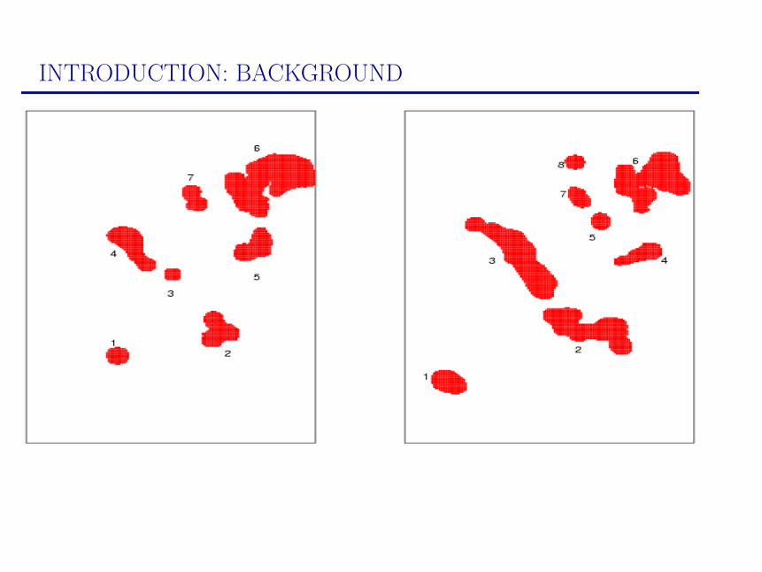
INTRODUCTION: BACKGROUND
INTRODUCTION: OUTLINE
• Localization performance measures
• Metrics and notation
• Baddeley’s Delta Metric
• Using Baddeley’s Delta Metric for object matching and merging
• Results from two image pairs
• Future and Ongoing Work
3
Localization performance measures
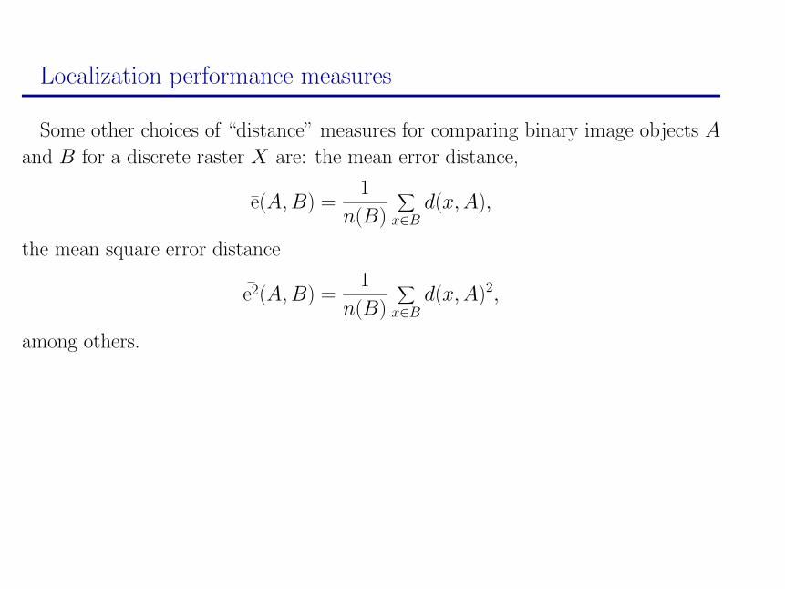
Some other choices of “distance” measures for comparing binary image objects A
and B for a discrete raster X are: the mean error distance,
e(A, B) =1
n(B)
∑x∈B
d(x, A),
the mean square error distance
e2(A, B) =1
n(B)
∑x∈B
d(x, A)2,
among others.
4
Localization performance measures: some problems
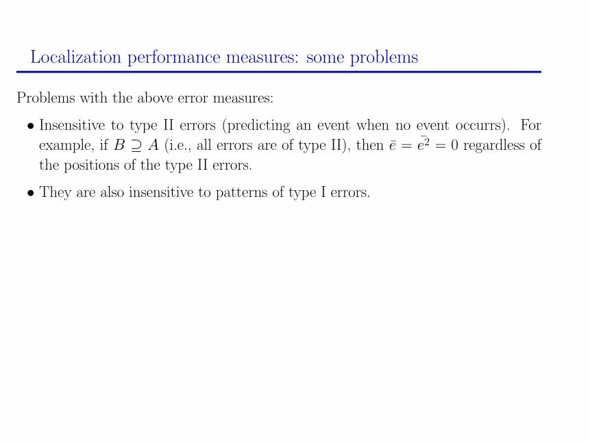
Problems with the above error measures:
• Insensitive to type II errors (predicting an event when no event occurrs). For
example, if B ⊇ A (i.e., all errors are of type II), then e = e2 = 0 regardless of
the positions of the type II errors.
• They are also insensitive to patterns of type I errors.
5
Metrics and notation
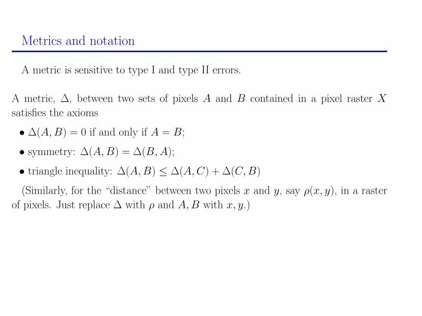
A metric is sensitive to type I and type II errors.
A metric, ∆, between two sets of pixels A and B contained in a pixel raster X
satisfies the axioms
• ∆(A, B) = 0 if and only if A = B;
• symmetry: ∆(A, B) = ∆(B, A);
• triangle inequality: ∆(A, B) ≤ ∆(A, C) + ∆(C, B)
(Similarly, for the “distance” between two pixels x and y, say ρ(x, y), in a raster
of pixels. Just replace ∆ with ρ and A, B with x, y.)
6
Metrics and notation
Let d(x, A) denote the shortest distance from pixel x to A ⊆ X . That is,
d(x, A) = min{ρ(x, a) : a ∈ A}
Also, d(x, Ø) ≡ ∞.
7
Metrics and notation
d(·, A) can be computed rapidly by the distance transform algorithm. See, for ex-
ample:
Borgefors, G. Distance transformations in digital images. Computer Vision, Graph-
ics and Image Processing, 34:344–371, 1986.
Rosenfeld and Pfalz, J.L. Sequential operations in digital picture processing. Jour-
nal of the Association for Computing Machinery, 13:471, 1966.
Rosenfeld and Pfalz, J.L. Distance functions on digital pictures. Pattern Recogni-
tion, 1:33–61, 1968.
8
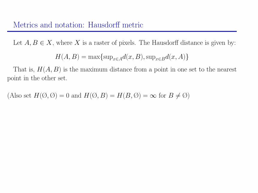
Metrics and notation: Hausdorff metric
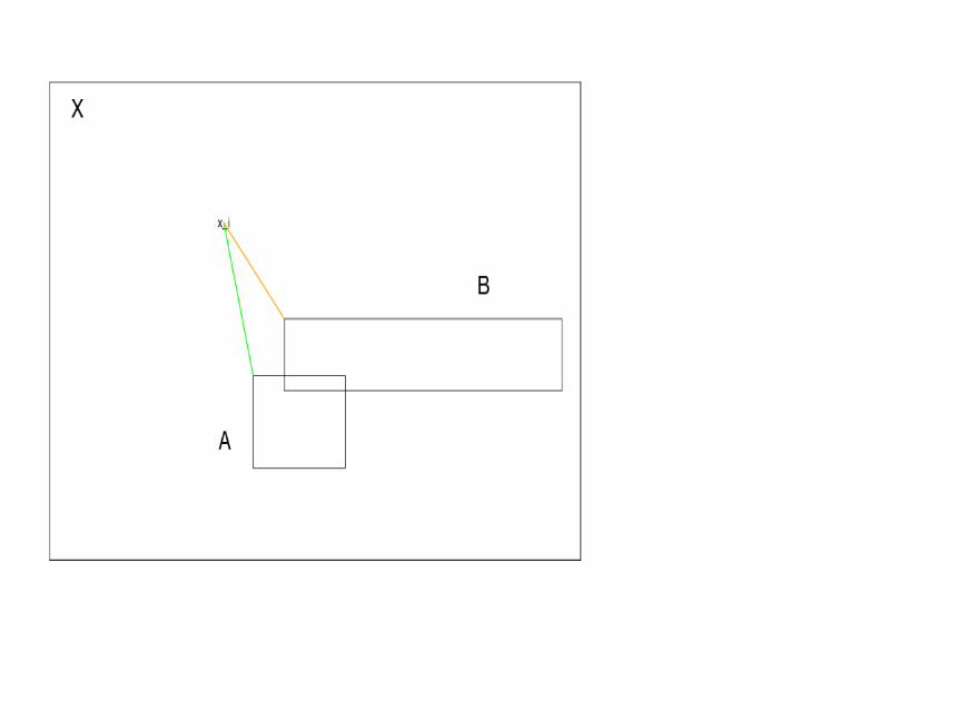
Let A, B ∈ X , where X is a raster of pixels. The Hausdorff distance is given by:
H(A, B) = max{supx∈Ad(x, B), supx∈Bd(x, A)}
That is, H(A, B) is the maximum distance from a point in one set to the nearest
point in the other set.
(Also set H(Ø, Ø) = 0 and H(Ø, B) = H(B, Ø) = ∞ for B 6= Ø)
9
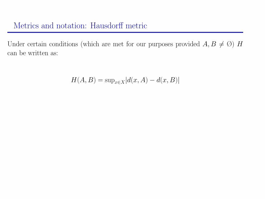
Metrics and notation: Hausdorff metric
Under certain conditions (which are met for our purposes provided A, B 6= Ø) H
can be written as:
H(A, B) = supx∈X|d(x, A)− d(x, B)|
10
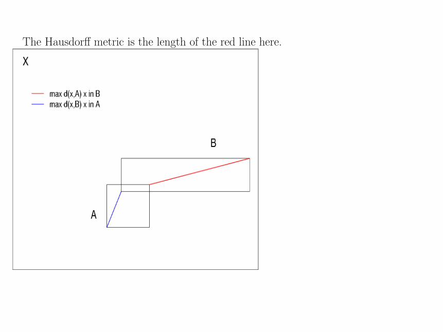
The Hausdorff metric is the length of the red line here.
11
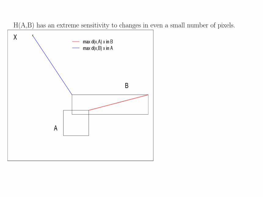
H(A,B) has an extreme sensitivity to changes in even a small number of pixels.
12
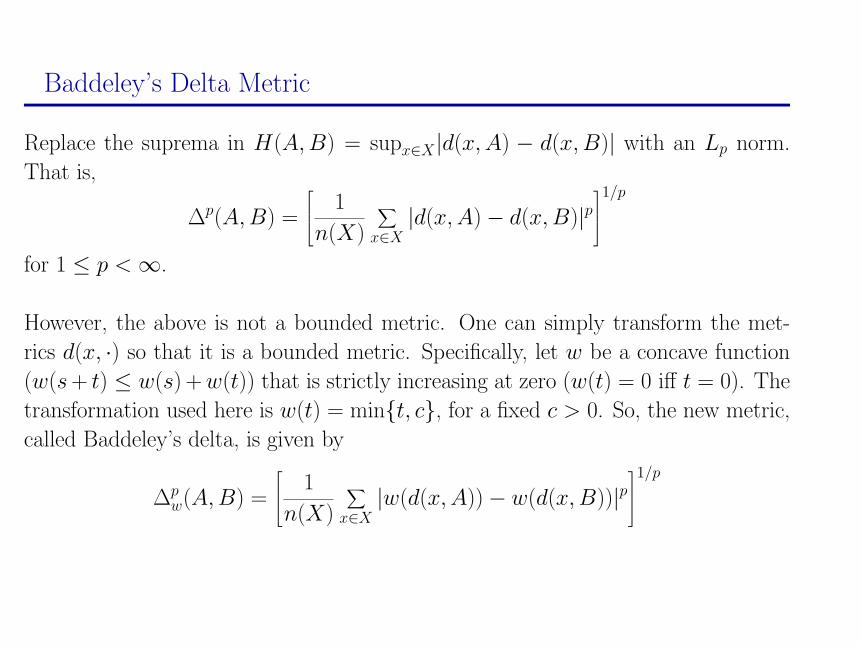
Baddeley’s Delta Metric
Replace the suprema in H(A, B) = supx∈X|d(x, A) − d(x, B)| with an Lp norm.
That is,
∆p(A, B) =
1
n(X)
∑x∈X
|d(x, A)− d(x, B)|p1/p
for 1 ≤ p < ∞.
However, the above is not a bounded metric. One can simply transform the met-
rics d(x, ·) so that it is a bounded metric. Specifically, let w be a concave function
(w(s + t) ≤ w(s) + w(t)) that is strictly increasing at zero (w(t) = 0 iff t = 0). The
transformation used here is w(t) = min{t, c}, for a fixed c > 0. So, the new metric,
called Baddeley’s delta, is given by
∆pw(A, B) =
1
n(X)
∑x∈X
|w(d(x, A))− w(d(x, B))|p1/p
13
14
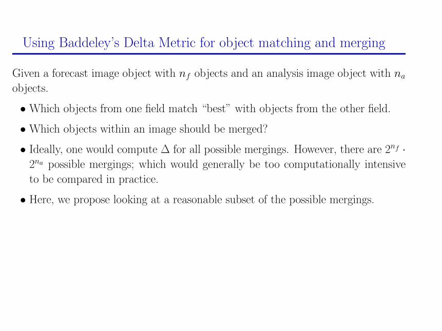
Using Baddeley’s Delta Metric for object matching and merging
Given a forecast image object with nf objects and an analysis image object with na
objects.
• Which objects from one field match “best” with objects from the other field.
• Which objects within an image should be merged?
• Ideally, one would compute ∆ for all possible mergings. However, there are 2nf ·2na possible mergings; which would generally be too computationally intensive
to be compared in practice.
• Here, we propose looking at a reasonable subset of the possible mergings.
15
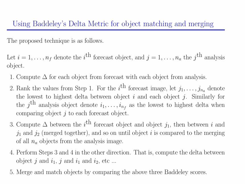
Using Baddeley’s Delta Metric for object matching and merging
The proposed technique is as follows.
Let i = 1, . . . , nf denote the ith forecast object, and j = 1, . . . , na the jth analysis
object.
1. Compute ∆ for each object from forecast with each object from analysis.
2. Rank the values from Step 1. For the ith forecast image, let j1, . . . , jna denote
the lowest to highest delta between object i and each object j. Similarly for
the jth analysis object denote i1, . . . , infas the lowest to highest delta when
comparing object j to each forecast object.
3. Compute ∆ between the ith forecast object and object j1, then between i and
j1 and j2 (merged together), and so on until object i is compared to the merging
of all na objects from the analysis image.
4. Perform Steps 3 and 4 in the other direction. That is, compute the delta between
object j and i1, j and i1 and i2, etc ...
5. Merge and match objects by comparing the above three Baddeley scores.
16
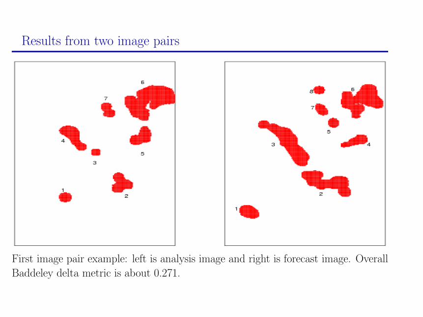
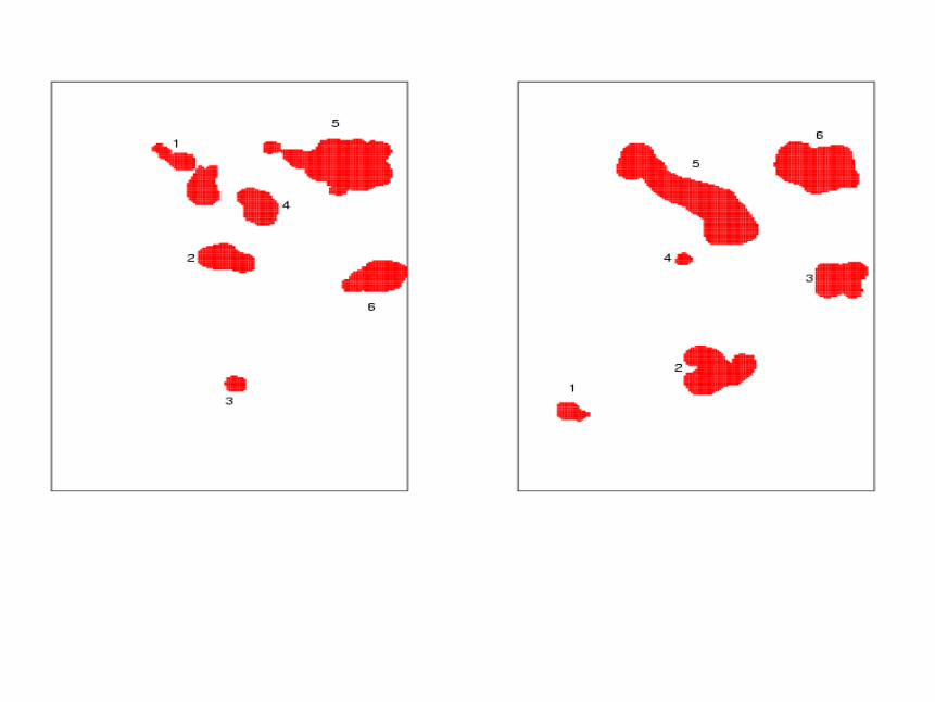
Results from two image pairs
First image pair example: left is analysis image and right is forecast image. Overall
Baddeley delta metric is about 0.271.
17
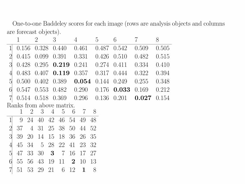
One-to-one Baddeley scores for each image (rows are analysis objects and columns
are forecast objects).1 2 3 4 5 6 7 8
1 0.156 0.328 0.440 0.461 0.487 0.542 0.509 0.505
2 0.415 0.099 0.391 0.331 0.426 0.510 0.482 0.515
3 0.428 0.295 0.219 0.241 0.274 0.411 0.334 0.410
4 0.483 0.407 0.119 0.357 0.317 0.444 0.322 0.394
5 0.500 0.402 0.389 0.054 0.144 0.249 0.255 0.348
6 0.547 0.553 0.482 0.290 0.176 0.033 0.169 0.212
7 0.514 0.518 0.369 0.296 0.136 0.201 0.027 0.154Ranks from above matrix.
1 2 3 4 5 6 7 8
1 9 24 40 42 46 54 49 48
2 37 4 31 25 38 50 44 52
3 39 20 14 15 18 36 26 35
4 45 34 5 28 22 41 23 32
5 47 33 30 3 7 16 17 27
6 55 56 43 19 11 2 10 13
7 51 53 29 21 6 12 1 8
18
19
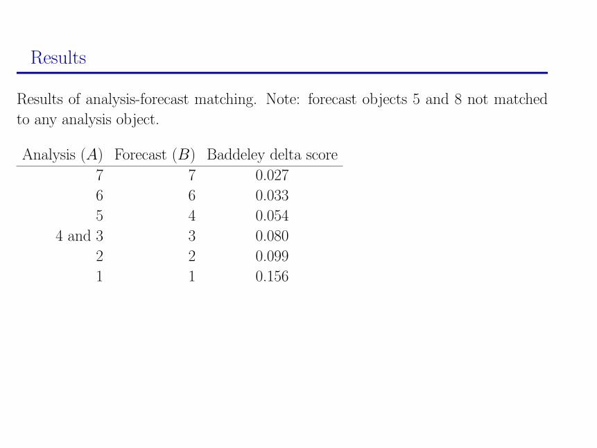
Results
Results of analysis-forecast matching. Note: forecast objects 5 and 8 not matched
to any analysis object.
Analysis (A) Forecast (B) Baddeley delta score
7 7 0.027
6 6 0.033
5 4 0.054
4 and 3 3 0.080
2 2 0.099
1 1 0.156
20

21
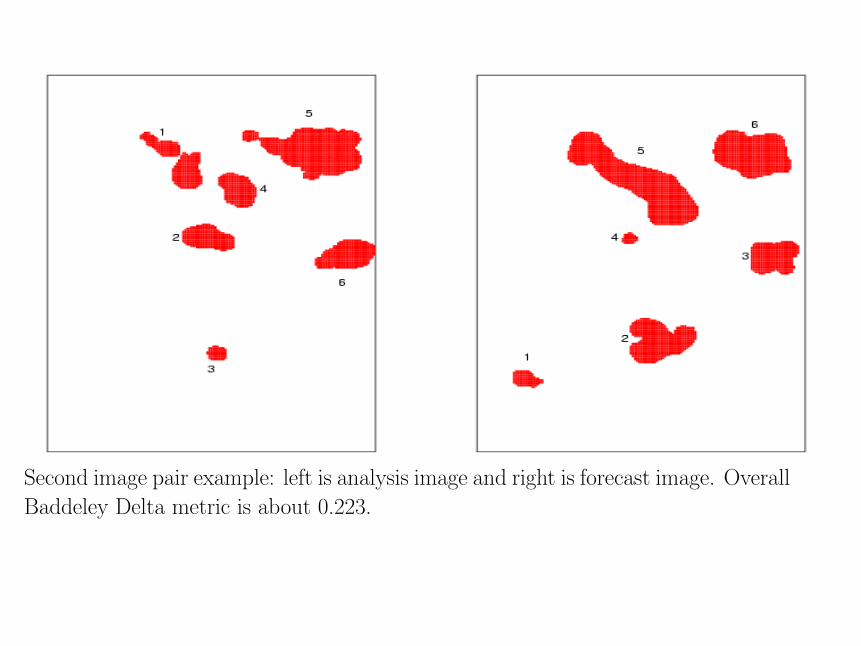
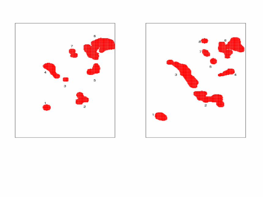
Second image pair example: left is analysis image and right is forecast image. Overall
Baddeley Delta metric is about 0.223.
22
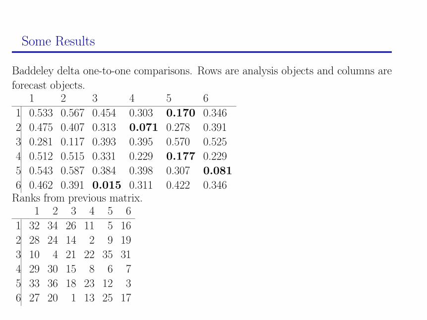
Some Results
Baddeley delta one-to-one comparisons. Rows are analysis objects and columns are
forecast objects.1 2 3 4 5 6
1 0.533 0.567 0.454 0.303 0.170 0.346
2 0.475 0.407 0.313 0.071 0.278 0.391
3 0.281 0.117 0.393 0.395 0.570 0.525
4 0.512 0.515 0.331 0.229 0.177 0.229
5 0.543 0.587 0.384 0.398 0.307 0.081
6 0.462 0.391 0.015 0.311 0.422 0.346Ranks from previous matrix.
1 2 3 4 5 6
1 32 34 26 11 5 16
2 28 24 14 2 9 19
3 10 4 21 22 35 31
4 29 30 15 8 6 7
5 33 36 18 23 12 3
6 27 20 1 13 25 17
23
24
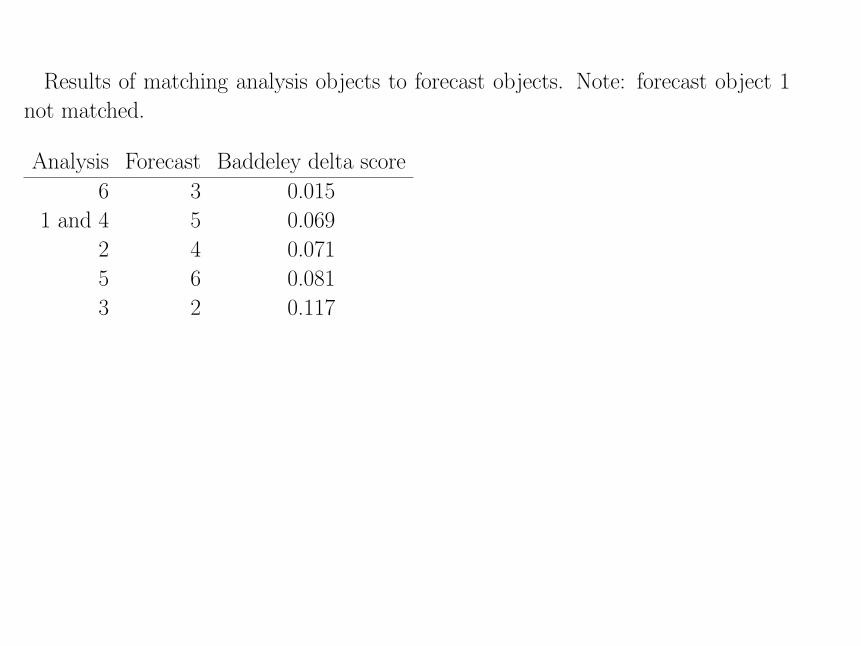
Results of matching analysis objects to forecast objects. Note: forecast object 1
not matched.
Analysis Forecast Baddeley delta score
6 3 0.015
1 and 4 5 0.069
2 4 0.071
5 6 0.081
3 2 0.117
25

26
Future and Ongoing Work
• How to combine information from “best” matches/merges to give a summary
score based on the Baddeley delta.
• What constitutes a “good” Baddeley delta score (have a human expert judge
several cases?).
• How to incorporate into overall verification scheme.
• Characteristics/distributions of ∆’s.
• How to compare with Fuzzy Logic analysis of Bullock et al.
27
References
Baddeley, A.J., 1992: Errors in binary images and an Lp version of the Hausdorff
metric, Nieuw Archief voor Wiskunde, 10: 157–183.
Baddeley, A.J., 1992: An error metric for binary images, In W. Forstner and S.
Ruwiedel (ed.) Robust Computer Vision Algorithms, Proceedings, Interna-
tional Workshop on Robust Computer Vision, Bonn. Karlsruhe: Wichmann,
59–78.See: http://www.maths.uwa.edu.au/~adrian/metrics.html
28


