velocity analysis - home: earth and...
TRANSCRIPT
1
Velocity analysisVelocity analysis

2
Effect of stacking on incoherent noise
Tools for Velocity Analysis
Constant velocity gather
CMP gather is NMO corrected at single low velocity for whole gather. Repeated for many other velocities.All gathers are laid side-by-side.
Disadvantages: poor resolution, only good SNR events can bechecked
Constant Velocity Stack (CVS)
similar to CVG, stacks instead of gather
Disadvantages: as CVG but you don’t even look at actual data
original correct overcorrected undercorrected

3
Tools for Velocity Analysis
Velocity Spectrum or Semblance
best modern method – Industry standard
define time window in which wavelet is containedcalculate hyperbolic trajectorymeasure coherency of trace signal, e.g. semblance
∑ ∑
∑ ∑
k M
k M
a
a
M 2
2
1 k – samples in time windowM – traces across gather
Tools for Velocity Analysis
contour semblance statistics as function of intercept time and stacking velocity
peaks show actual intercept time and velocity
advantage: optimal resolutionweak and strong events
disadvantage: none (as long as software allows interactive picking and displaying of results)
Velocity spectra can be distorted in areas with static problems

4
Stacking Velocity VS
Is the velocity that you have to put into the NMO equations such that the CMP gather stacks (adds) together best, i.e. the velocity that allows the best fit of the travel time curve on a CMP gather to the hyperbola within the spread length.Approximately equal to VRMS for small spreads
a) Actual data move-out
b) Best-fitting hyperbola
(stacking velocity)VNMO=VRMS
c) NMO approximation
(short spread)VNMO= VS
Multiple horizontal layers
Root-Mean-Square Velocity
21
2
=
∑
∑
N
i
N
ii
RMSt
tv
VN
ti= travel time through i-th layer
0
2
2
2 TV
xT
RMS
N ≈∆
NMO
x
5
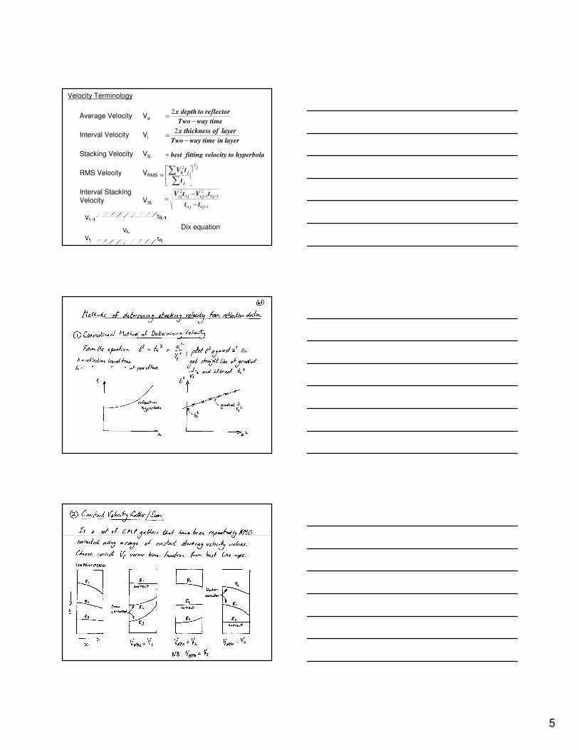
Velocity Terminology
Average Velocity Va
Interval Velocity Vi
Stacking Velocity VS
RMS Velocity VRMS
Interval StackingVelocity VIS
timewayTwo
reflectortodepthx
−=
2
layerintimewayTwo
layerofthicknessx
−=
2
hyperbolatovelocityfittingbest=
21
2
=
∑∑
j
jij
t
tV
100
10
2
10
2
−
−−
−
−=
jj
jjsjjs
tt
tVtV
Dix equation
6
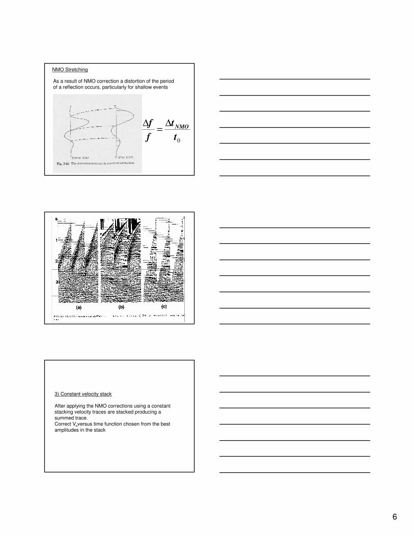
NMO Stretching
0t
t
f
f NMO∆=
∆
As a result of NMO correction a distortion of the periodof a reflection occurs, particularly for shallow events
3) Constant velocity stack
After applying the NMO corrections using a constantstacking velocity traces are stacked producing asummed trace.Correct Vsversus time function chosen from the bestamplitudes in the stack

7

8

9
Multiple
suppression
post-stack
processing
In general, it’s likely that multiples have a slower NMO velocity than primaries at the same TWT
So if the primary is properly corrected, multiples will be
under-corrected (“v” is too big in x2/2v2t0)
�

10
Corrected gathers can be put into FK domain
Primaries plot on K=0 axis, multiple plot at range of +ve K
If a stacking velocity function between
primaries & multiples is used, primaries & multiples are over- and
under-corrected, so plot into opposite halves of K space

11