applied engineering problem solving lesson #4: numerical...
TRANSCRIPT
1
Applied Engineering Problem Solving
Lesson #4: Numerical Error
Prof. John R. White
Chemical and Nuclear Engineering
UMass-Lowell, Lowell MA
(Oct. 2017)CHEN.3170 Applied Engineering Problem Solving
Lesson 4: Numerical Error
Lesson #4 Goals
Computer representation of numbers
(just the basics)
Round-off error and machine precision
Implication of round-off error in iterative
techniques
Taylor series expansions and the
truncation error associated with a finite
approximation to infinite series (FD
approximation to derivatives)
Trade-offs associated with round-off and
truncation errors
Numerical Error: Round-Off and Truncation Error…
Gilat:
none
Chapra:
Chapter 4
Lesson # 4 Lecture Notes
and Illustrative Examples
(Oct. 2017)CHEN.3170 Applied Engineering Problem Solving
Lesson 4: Numerical Error
2
Numerical Error
Round-Off Error
Due to the fact that computers can only represent
quantities with a finite number of digits
Truncation Error
Associated with the approximations that are
usually required when attempting to represent an
exact mathematical expression or operation
Floating point arithmetic is NOT exact…
(Oct. 2017)CHEN.3170 Applied Engineering Problem Solving
Lesson 4: Numerical Error
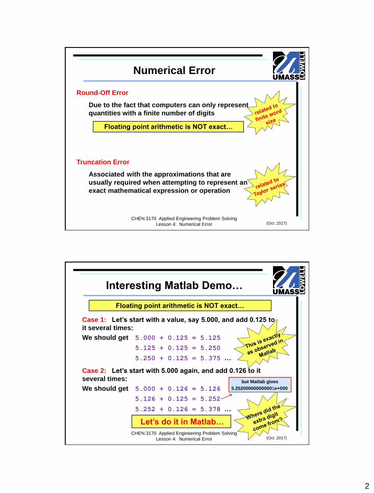
Interesting Matlab Demo…
Case 1: Let’s start with a value, say 5.000, and add 0.125 to
it several times:
We should get 5.000 + 0.125 = 5.125
5.125 + 0.125 = 5.250
5.250 + 0.125 = 5.375 …
Case 2: Let’s start with 5.000 again, and add 0.126 to it
several times:
We should get 5.000 + 0.126 = 5.126
5.126 + 0.125 = 5.252
5.252 + 0.126 = 5.378 …
Floating point arithmetic is NOT exact…
Let’s do it in Matlab…
but Matlab gives
5.252000000000001e+000
(Oct. 2017)CHEN.3170 Applied Engineering Problem Solving
Lesson 4: Numerical Error
3
Computer Representation of Numbers
Base 10 Arithmetic:
and
Thus, x.y could be written as …b5b4b3b2b1b0 . c1c2c3… using
base 10 notation.
Human computers do
arithmetic in base 10
kk
k 0
x b 10
k
k
k 1
y c 10
0 1 2 35.125 5 10 . 1 10 2 10 5 10
0 1 2 35.126 5 10 . 1 10 2 10 6 10
(Oct. 2017)CHEN.3170 Applied Engineering Problem Solving
Lesson 4: Numerical Error
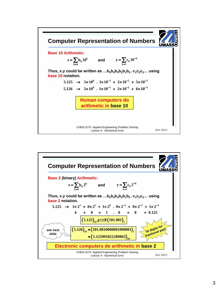
Computer Representation of Numbers
Base 2 (binary) Arithmetic:
and
Thus, x.y could be written as …b5b4b3b2b1b0 . c1c2c3… using
base 2 notation.
Electronic computers do arithmetic in base 2
kk
k 0
x b 2
k
k
k 1
y c 2
2 1 0 1 2 35.125 1 2 0 2 1 2 . 0 2 0 2 1 2
4 0 1 . 0 0 0.125
10 2
5.125 101.001
10 2
10
5.126 101.0010000001000001
5.125991821289063
see next
slide
(Oct. 2017)CHEN.3170 Applied Engineering Problem Solving
Lesson 4: Numerical Error
4
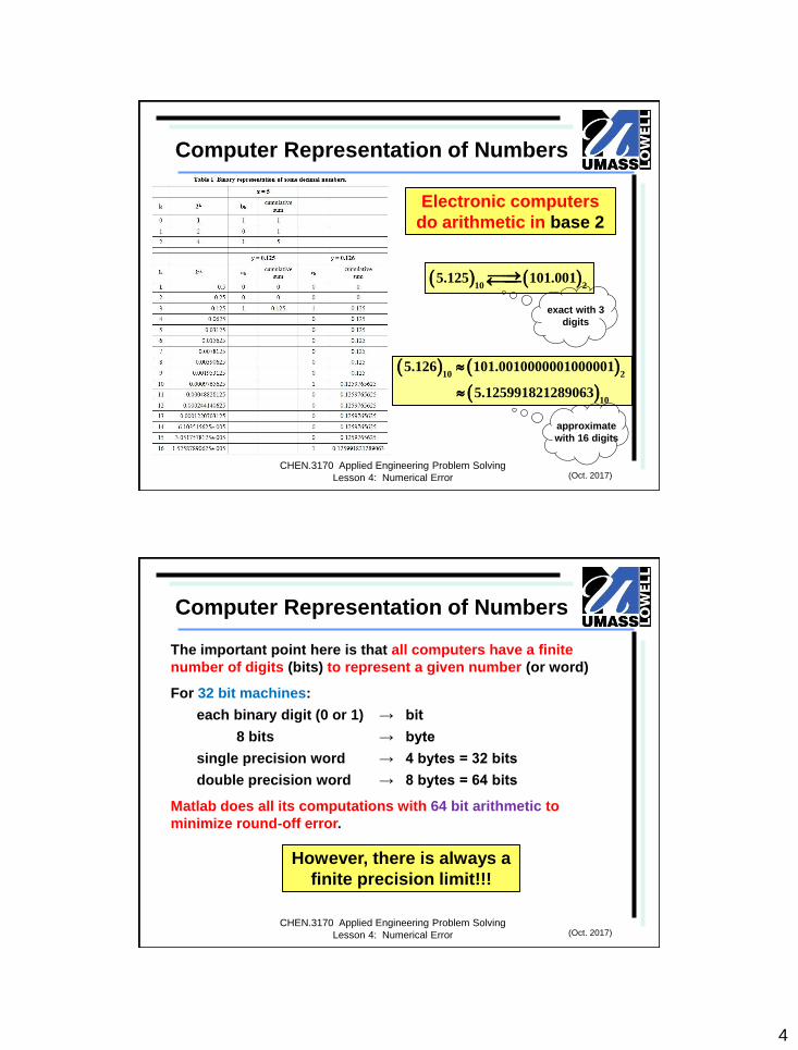
Computer Representation of Numbers
Electronic computers
do arithmetic in base 2
10 2
10
5.126 101.0010000001000001
5.125991821289063
10 2
5.125 101.001
exact with 3
digits
approximate
with 16 digits
(Oct. 2017)CHEN.3170 Applied Engineering Problem Solving
Lesson 4: Numerical Error
The important point here is that all computers have a finite
number of digits (bits) to represent a given number (or word)
For 32 bit machines:
each binary digit (0 or 1) → bit
8 bits → byte
single precision word → 4 bytes = 32 bits
double precision word → 8 bytes = 64 bits
Matlab does all its computations with 64 bit arithmetic to
minimize round-off error.
Computer Representation of Numbers
However, there is always a
finite precision limit!!!
(Oct. 2017)CHEN.3170 Applied Engineering Problem Solving
Lesson 4: Numerical Error

5
This precision limit is characterized by a number called
machine epsilon, m.
It is defined precisely as the smallest floating point number, m,
such that
We can easily estimate machine epsilon, m, on any computer
by continually reducing a number (say, by a factor of two) until
the above condition is no longer valid.
epsilon = 1.0;
while epsilon + 1.0 > 1.0
epsilon = epsilon/2;
end
Matlab has a built-in variable, eps, to store this value…
Machine Epsilon, m
see meps.m
m1 1
(Oct. 2017)CHEN.3170 Applied Engineering Problem Solving
Lesson 4: Numerical Error
Although proper algorithm design and 64-bit arithmetic tend to
minimize round off error, it is always something that you
should be aware of when doing numerical computations and
code development.
Because of round off error, we almost never ask the question
“Is x = y?”.
Instead, we ask “Is x close to y?” and this is often implemented
as follows:
rerr = 1; tol = 1e-5;
while rerr > tol
continue calculation that updates x and/or y
rerr = abs((x-y)/y);
end
where tol is some user-defined tolerance…
Ramifications of Round-Off Error…
(Oct. 2017)CHEN.3170 Applied Engineering Problem Solving
Lesson 4: Numerical Error
6
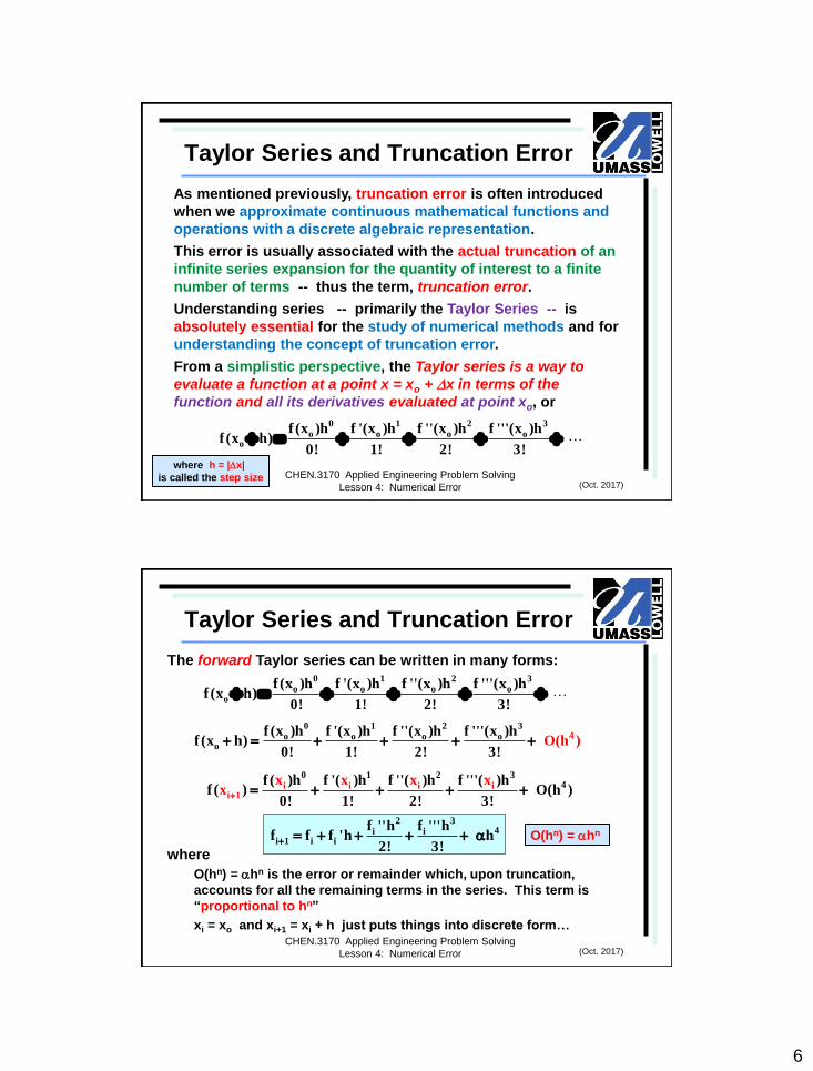
As mentioned previously, truncation error is often introduced
when we approximate continuous mathematical functions and
operations with a discrete algebraic representation.
This error is usually associated with the actual truncation of an
infinite series expansion for the quantity of interest to a finite
number of terms -- thus the term, truncation error.
Understanding series -- primarily the Taylor Series -- is
absolutely essential for the study of numerical methods and for
understanding the concept of truncation error.
From a simplistic perspective, the Taylor series is a way to
evaluate a function at a point x = xo + x in terms of the
function and all its derivatives evaluated at point xo, or
Taylor Series and Truncation Error
0 1 2 3o o o o
o
f (x )h f '(x )h f ''(x )h f '''(x )hf (x h)
0! 1! 2! 3!
where h = |x|
is called the step size(Oct. 2017)
CHEN.3170 Applied Engineering Problem Solving
Lesson 4: Numerical Error
The forward Taylor series can be written in many forms:
where
O(hn) = hn is the error or remainder which, upon truncation,
accounts for all the remaining terms in the series. This term is
“proportional to hn”
xi = xo and xi+1 = xi + h just puts things into discrete form…
Taylor Series and Truncation Error
0 1 2 3o o o o
o
f (x )h f '(x )h f ''(x )h f '''(x )hf (x h)
0! 1! 2! 3!
O(hn) = hn
0 1 2 3o o o o
o4f (x )h f '(x )h f ''(x )h f '''(x )h
f (x h)0! 1! 2! 3!
O(h )
0 1i
2 34i i i
i 1
f ( )h f '( )h f ''( )h f '''( )hf ( ) O(h )
0! 1! 2! 3!
x x x xx
2 34i i
i 1 i i
f ''h f '''hf f f 'h h
2! 3!
(Oct. 2017)CHEN.3170 Applied Engineering Problem Solving
Lesson 4: Numerical Error

7
For f(x) = ex with the reference point at xo = 0, the forward
Taylor series
becomes
But, now we can let h = x for convenience of notation.
Thus,
Similarly,
Example of Round-Off & Truncation Error
0 1 2 3o o o o
o
f (x )h f '(x )h f ''(x )h f '''(x )hf (x h)
0! 1! 2! 3!
1 2 3h 1 h h h
f (h) e0! 1! 2! 3!
since dn(ex)/dxn = ex
and e0 = 1
2 3 4 nx
n 0
x x x xe 1 x
2! 3! 4! n!
2 3 4 n nx
n 0
x x x ( 1) xe 1 x
2! 3! 4! n!
(Oct. 2017)CHEN.3170 Applied Engineering Problem Solving
Lesson 4: Numerical Error
Consider the computation of e3 and e-3 using the Taylor series
truncated to 8 terms with only 5 significant digits in our
calculations.
Doing the calculations gives:
Case 1:
and my calculator gives e3 = 20.086 -- thus, our 8-term estimate
has an error of about –1.2% .
This error is dominated by truncation error, with only a minor loss
in accuracy associated with rounding the individual calculations
to 5 figures -- that is, the addition of a few more terms in the
series would give very accurate results.
Example of Round-Off & Truncation Error
3 9 27 81 243 729 2187e 1 3
2 6 24 120 720 5040
1 3 4.5 4.5 3.375 2.025 1.0125 0.43393 19.846
(Oct. 2017)CHEN.3170 Applied Engineering Problem Solving
Lesson 4: Numerical Error
8
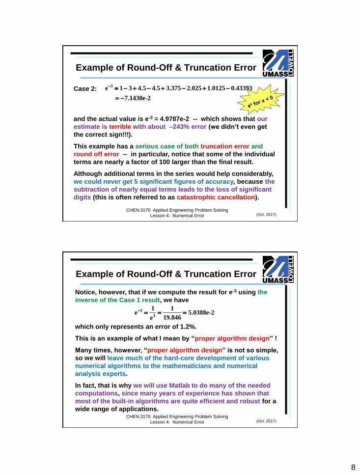
Case 2:
and the actual value is e-3 = 4.9787e-2 -- which shows that our
estimate is terrible with about –243% error (we didn’t even get
the correct sign!!!).
This example has a serious case of both truncation error and
round off error -- in particular, notice that some of the individual
terms are nearly a factor of 100 larger than the final result.
Although additional terms in the series would help considerably,
we could never get 5 significant figures of accuracy, because the
subtraction of nearly equal terms leads to the loss of significant
digits (this is often referred to as catastrophic cancellation).
Example of Round-Off & Truncation Error
3e 1 3 4.5 4.5 3.375 2.025 1.0125 0.43393
7.1430e-2
(Oct. 2017)CHEN.3170 Applied Engineering Problem Solving
Lesson 4: Numerical Error
Notice, however, that if we compute the result for e-3 using the
inverse of the Case 1 result, we have
which only represents an error of 1.2%.
This is an example of what I mean by “proper algorithm design” !
Many times, however, “proper algorithm design” is not so simple,
so we will leave much of the hard-core development of various
numerical algorithms to the mathematicians and numerical
analysis experts.
In fact, that is why we will use Matlab to do many of the needed
computations, since many years of experience has shown that
most of the built-in algorithms are quite efficient and robust for a
wide range of applications.
Example of Round-Off & Truncation Error
3
3
1 1e 5.0388e-2
19.846e
(Oct. 2017)CHEN.3170 Applied Engineering Problem Solving
Lesson 4: Numerical Error
9
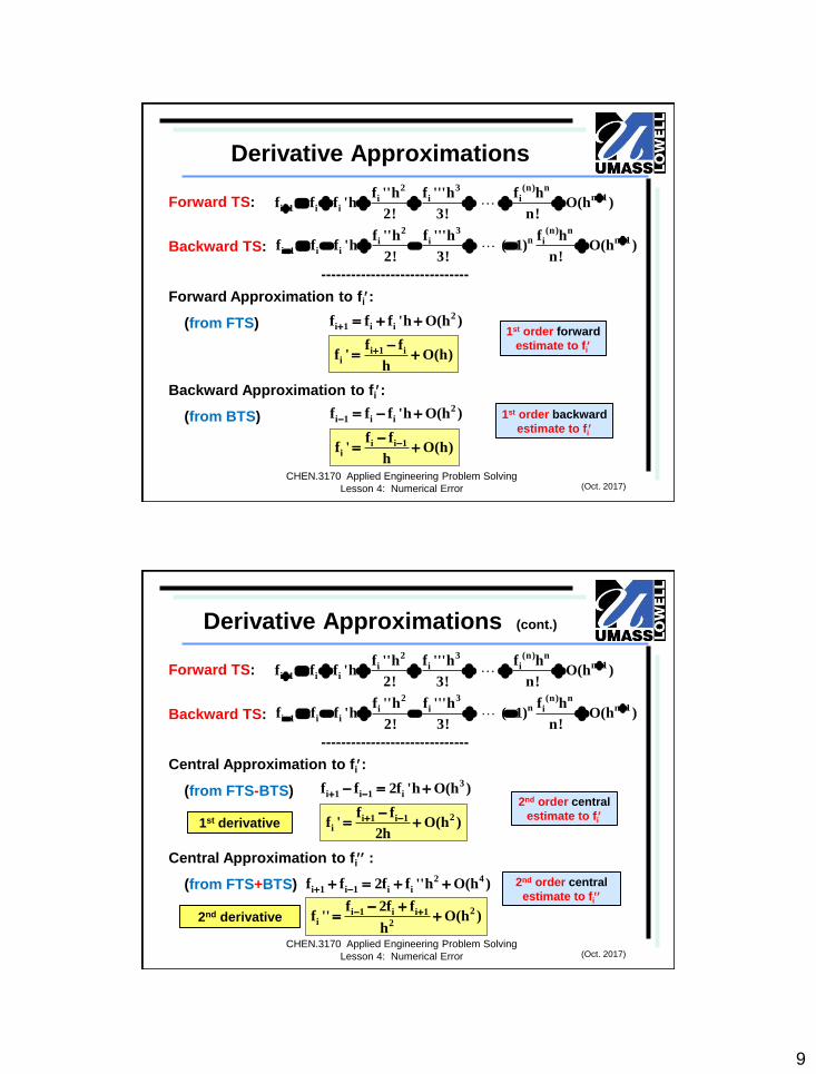
Forward TS:
Backward TS:
------------------------------
Forward Approximation to fi:
(from FTS)
Backward Approximation to fi:
(from BTS)
Derivative Approximations
2 3 (n) nn 1i i i
i 1 i i
f ''h f '''h f hf f f 'h O(h )
2! 3! n!
2 3 (n) nn n 1i i i
i 1 i i
f ''h f '''h f hf f f 'h ( 1) O(h )
2! 3! n!
2i 1 i if f f 'h O(h )
i 1 ii
f ff ' O(h)
h
2i 1 i if f f 'h O(h )
i i 1i
f ff ' O(h)
h
1st order forward
estimate to fi
1st order backward
estimate to fi
(Oct. 2017)CHEN.3170 Applied Engineering Problem Solving
Lesson 4: Numerical Error
Forward TS:
Backward TS:
------------------------------
Central Approximation to fi:
(from FTS-BTS)
Central Approximation to fi :
(from FTS+BTS)
Derivative Approximations (cont.)
2 3 (n) nn 1i i i
i 1 i i
f ''h f '''h f hf f f 'h O(h )
2! 3! n!
2 3 (n) nn n 1i i i
i 1 i i
f ''h f '''h f hf f f 'h ( 1) O(h )
2! 3! n!
3i 1 i 1 if f 2f 'h O(h )
2i 1 i 1i
f ff ' O(h )
2h
2i 1 i i 1i 2
f 2f ff '' O(h )
h
2nd order central
estimate to fi
2nd order central
estimate to fi
2 4i 1 i 1 i if f 2f f ''h O(h )
1st derivative
2nd derivative
(Oct. 2017)CHEN.3170 Applied Engineering Problem Solving
Lesson 4: Numerical Error

10
Let’s estimate, using some FD approximations, the
1st and 2nd derivatives of ex at x = 0
Example with Derivative Approximations
see deriv_approx.m
again dn(ex)/dxn = ex and e0 = 1
(Oct. 2017)CHEN.3170 Applied Engineering Problem Solving
Lesson 4: Numerical Error
Truncation error is often “proportional to the step size to some
power n”, or
The order of error, n , can often be estimated via a set of
numerical experiments that use different step sizes.
For example, a plot of vs. h on a log-log scale gives a straight
line with slope n:
Or, with just two separate evaluations, we have
Order of Error from Numerical Tests
nh
n nlog log h log logh log nlogh
n n1 1 2 2h and h
nn1 21 1 1
n2 2 1 22
logh hor n
h log h hh
(Oct. 2017)CHEN.3170 Applied Engineering Problem Solving
Lesson 4: Numerical Error
11
Reducing the step size, h, is the most common way to reduce
truncation error.
However, this often leads to an increased number of
computations and, since round-off error is accumulative, more
floating point arithmetic leads to more round-off error.
Truncation vs. Round-off Errors
This is illustrated in the
sketch, where the total
error is simply the sum of
the truncation and round-
off errors.
However, for most
practical engineering
problems, the truncation
error dominates.
normal
operation
(Oct. 2017)CHEN.3170 Applied Engineering Problem Solving
Lesson 4: Numerical Error
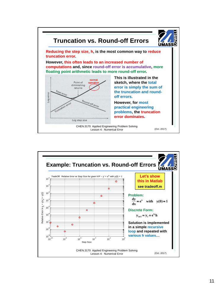
Problem:
Discrete Form:
Solution is implemented
in a simple recursive
loop and repeated with
various h values…
Example: Truncation vs. Round-off Errors
Let’s show
this in Matlab
see tradeoff.m
xdye with y(0) 1
dx
ix
i 1 iy y e h
10-10
10-8
10-6
10-4
10-2
100
10-9
10-8
10-7
10-6
10-5
10-4
10-3
10-2
10-1
TradeOff: Relative Error vs Step Size for given IVP -- y' = ex with y(0) = 1
Step Size
Rela
tive E
rror
in y
f = y
(xf)
= y
(2)
(Oct. 2017)CHEN.3170 Applied Engineering Problem Solving
Lesson 4: Numerical Error

12
More Illustrative Examples
On Evaluating Infinite Series – An Example
Example that illustrates how to generate a Taylor
series for f(x) = sinh(x) and on how to efficiently
evaluate this infinite power series in Matlab.
Algorithm to Evaluate Infinite Power Series
Set maxT and tol for stopping the calculation (also set > tol)
Initialize counter and first term -- set n = 1 and T = T1
Initialize the partial sum to the first term -- set f = T
while > tol && n < maxT
compute r, where rn = Tn+1/Tn (specific to function of interest)
T = r*T (compute next term in series)
f = f + T (update partial sum)
= max(abs(T/f)) (compute maximum relative change)
n = n + 1 (increment counter)
end
see
infinite_series.pdf
3 5 2n 1
n 1
x x xf (x) sinhx x
3! 5! (2n 1)!
Can you
derive this?
(Oct. 2017)CHEN.3170 Applied Engineering Problem Solving
Lesson 4: Numerical Error
How do we compute rn?
For the specific case of f(x) = sinh(x):
Thus rn becomes
where we have used the fact that
3 5 2n 1
n 1
x x xf (x) sinhx x
3! 5! (2n 1)!
2(n 1) 1n 1
n 2n 1n
2 2n 1 2
2n 1
2n 1 !T xr
T 2(n 1) 1 ! x
2n 1 !x x x
2n 1 2n 2n 1 ! 2n 1 2nx
2(n 1) 1 ! 2n 2 1 ! 2n 1 ! 2n 1 2n 2n 1 !
again, see infinite_series.pdf for the detailed
development and implementation within Matlab
(Oct. 2017)CHEN.3170 Applied Engineering Problem Solving
Lesson 4: Numerical Error

13
0 1 2 3 4 5 6 7 8 9 100
20
40
60
80
100
120PlaneWall_1: Plate Temperature Profile at Various Times
Distance (cm)
Tem
pera
ture
(C
)
0.0 sec
1.0 sec
5.0 sec
15.0 sec
30.0 sec
60.0 sec
More Illustrative Examples (cont.)
Evaluating and Plotting Space-Time Temperature Distributions
with 2nt
n n
n 1
T(x,t) a sin( x) e
in n
4T(2n 1)and a
2L (2n 1)
see
planewall_1.pdf(Oct. 2017)
CHEN.3170 Applied Engineering Problem Solving
Lesson 4: Numerical Error
More Illustrative Examples (cont.)
Introduction to Finite
Difference Methods
for Solution of ODEs
This is a BIGGIE -- we will emphasize
this in a separate presentation…
The goal here is to convert continuous differential
equations into discrete difference equations…
IVPs and BVPs are treated quite differently
IVPs lead to recursive equations
BVPs lead to simultaneous equations
Let’s look at the details…
(Oct. 2017)CHEN.3170 Applied Engineering Problem Solving
Lesson 4: Numerical Error