variation in the inflation experience of uk households
TRANSCRIPT
Page 1 of 84
Next release: To be announced
Release date: 15 December 2014
Contact: Philip [email protected]
Compendium
Variation in the Inflation Experience of UK Households: 2003-2014Estimates of the inflation rates experienced by different types of of household in the UK.
Chapters in this compendium
1. About this release
2. Executive summary
3. Methods, data and literature
4. Results
5. Housing costs
6. Democratic indices
7. Limitations
8. Conclusions
9. List of Appendices
10. References

Page 2 of 84
Next release: To be announced
Release date: 15 December 2014
Contact: Philip [email protected]
Compendium
About this releaseEstimates of the inflation rates experienced by different types of of household in the UK.
Table of contents
1. Abstract
2. Acknowledgements
3. Section 1. Introduction
4. Background notes

Page 3 of 84
1 . Abstract
This paper presents ONS analysis of the inflation rates experienced by different types of households in the UK between 2003 and 2014. Using micro-level data from the Living Costs and Food Survey (LCF) and national-level data from the Consumer Prices Index (CPI), it estimates price indices and inflation rates for households in different positions of the income and expenditure distributions, for households with and without children and for retired and non-retired households. It finds that the inflation experience of UK households differed widely over this period, with implications for economic policy. Low-spending households experienced faster rates of price increase than high-spending households. For the former group, prices increased by 3.3% per year on average between 2003 and 2013, while they increased by just 2.3% on average for the latter group. Inflation differentials for other sub-groups were smaller, although rates of price increase were faster for low-income households, retired households and households without children than for high-income, non-retired and households with children respectively. A ‘democratically-weighted’ price index was around 0.3 percentage points higher than the CPI on average over this period. This paper also sets out a range of areas for future analysis, among which an examination of how prices for specific products vary across households and the incorporation of housing costs are the most prominent.
2 . Acknowledgements
This paper has benefited from the input of a broad research team at ONS and the UKSA, including, but not limited to, Eric Crane, Rosemary Foster, Ainslie Restieaux, Richard Tonkin, Valerie Fender, Grisel.la Dial Pujol and Matthew Power. The authors are also grateful for comments and assistance from Peter Patterson, Ian Derrick, Richard Campbell, Giles Horsfield and Lorraine Haftowski, as well as Arthur Bennett, Ciaren Taylor and Fred Foxton. We also acknowledge the many useful comments provided by several external experts, including Martin Weale, from the Bank of England, and Peter Levell, of the Institute for Fiscal Studies. Any remaining mistakes or omissions remain our own.
3 . Section 1. Introduction
The Consumer Prices Index (CPI) is of central importance in macroeconomic analysis. Calculated each month using more than 180,000 price quotes, it is designed to capture the average price movement of the goods and services purchased by the household sector. However, because the consumption baskets of specific households differ and because prices do not all change at the same rate, the price experience of individual households may differ from the average shown in official statistics. In a similar manner to the average of any variable, some households will experience higher rates of inflation, while others will observe a lower rate of price increase. These differences are the subject of this paper.
The motivation for this work is three-fold. First, the estimation of inflation rates for different households has an intrinsic interest in and of itself. The rate of price change experienced by households of different types and at different points in the income and expenditure distribution can help policy-makers and researchers alike to understand their behaviour. The unusual nature of the 2003-2014 period – taking in phases of both economic expansion and contraction, of relatively high and low average inflation – heightens this interest. Secondly, the findings offer some important insights for debates on economic policy in the UK. Thirdly, this work has been a central focus of the Johnson Review, to be published in January 2015. This work has benefited from their insights and involvement throughout the process.

Page 4 of 84
1.
2.
Figure 1.1 shows the rate of annual inflation estimated using the CPI between January 2003 and October 2014. Between 2003 and 2006, the annual rate of price change was relatively stable: inflation varied around an average rate of 1.8% per month, between a low of 1.1% and a high of 3.0%. However, between 2007 and 2012, UK inflation was affected by a range of inter-related shocks including the global financial market shock, a substantial depreciation of the trade-weighted sterling exchange rate, volatile movements in commodity prices, and changes in the rate of VAT. All of these factors are likely to have contributed to a sharp increase in both the level and the variation of inflation. In the period since mid-2012, this pattern has reversed: the variation in inflation returned to its pre-downturn level, and the rate itself has now been within the Bank of England’s target range of 1.0% to 3.0% for the last 30 months. In particular, the moderation of inflation over the last ten months – shown in the shorter bars to the right of Figure 1.1 – appears to be partly a result of abating energy costs, movements in the exchange rate and falling food & drink prices.
Figure 1.1: Contributions to the annual rate of CPI inflation, % and percentage points
Source: ONS Calculations
Notes:
Stacked bars reflect the percentage point contributions of each of the 85 class-level items in the Classification of Individual Consumption by Purpose (COICOP) to the annual percentage change in the Consumer Prices Index (CPI). The contribution of each class-level item is estimated separately, before being aggregated to the categories above. Note that a reduction in the contribution of a series to the annual rate of change need not imply falling prices, but could also reflect a lower rate of increase.
Food, drink & tobacco is composed of food, non-alcoholic and alcoholic beverages and tobacco. Housing is composed of actual rents and products and services for the repair of dwellings. Elect., gas & fuel includes electricity, gas and other household fuels as well as fuels and lubricants for motor vehicles. Transport & package holidays includes passenger transport by road, rail, air and sea, as well as package holidays. Education reflects the division-level contribution. The ‘other’ category reflects the combined contributions of the remaining 56 class-level items and a small rounding error, bringing the sum of contributions to the CPI (ONS 2014a).

Page 5 of 84
Figure 1.1 also suggests that, as well as the recent moderation, much of the variation in the rate of inflation between 2003 and 2014 has been due to changes in the prices of energy and food & drink. These products account for a larger fraction of total spending for households with low levels of income or expenditure. As a consequence, households have differed in their exposure to these recent movements in prices, which in turn has influenced their experience of average price movements.
To assess the impact of these movements in prices and expenditure weights, this paper uses micro-level data from the Living Costs and Food Survey (LCF) and detailed data from CPI, to calculate price indices for individual groups of households, including households in different positions of the income and expenditure distributions, households with and without children, and retired and non-retired households. It sets out how expenditure patterns vary across each of these groups, examines how they drive differences in rates of price increase and assesses the impact of these differentials over the 2003-2014 period: encompassing periods of both relative stability and of substantial variation in the average inflation rate. It provides some evidence of the impact of housing costs on price pressure faced by households, and it presents a set of ‘democratically-weighted’ inflation rates that yield some information about the distribution of inflation outcomes in the UK .1
In so doing, this paper makes three significant contributions to the existing literature. First, it presents a more detailed analysis of CPI inflation rates for different sub-groups of the population than has previously been published, using expenditure weights at the class-level of the Classification of Individual Consumption According to Purpose (COICOP). Secondly, to the authors’ knowledge, it presents the first sub-group estimates of UK inflation that are directly comparable with the CPI. This involves both reconciling the household-level expenditure data with the expenditure weights used in the construction of the CPI, and using the same processing techniques to deliver a set of sub-group inflation rates which aggregate to the published CPI series. Finally, the paper provides a detailed discussion of methodological approaches in the field and identifies a range of ways in which the estimates presented here could be improved in the future.
The results of this paper have obvious implications for policy debates concerning the cost of living, the macroeconomic management of the economy as a whole and a range of wider issues. We conclude that rates of inflation differ across household types, with some of the largest differences existing between high- and low-expenditure households. Between 2002 and October 2014, prices increased 24.2 percentage points more for products consumed by households with the lowest levels of equivalised expenditure than for products consumed 2
by the highest spending households . By comparison, average prices for retired households and households 3
without children grew more quickly than non-retired and households with children respectively. Prices increased around 6.5 percentage points more quickly for the products purchased by the lowest compared with the highest-income groups in the period January 2002 to December 2013. Finally, we present evidence that a ‘democratically-weighted’ consumer prices index – which weights the price experience of each household equally – would have risen more sharply than the ‘plutocratically-weighted’ CPI – which draws on household sector expenditure weights – over this period. These results are summarised in Table 1.1 below:

Page 6 of 84
1.
2.
3.
1.
Table 1.1: Average annual inflation rates for selected groups, %, 2003-2013
%
Group Inflation
Decile of 1 2 9 10
Disposable Income 2.9 2.7 2.5 2.6
Expenditure 3.7 3.3 2.3 2.3
Households with Children 2.4
Households without Children 2.7
Retired Households 2.8
Non-Retired Households 2.5
‘Democratically-weighted’ 2.9
CPI 2.6
Source: ONS Calculations
Notes:
1. Deciles of disposable income and expenditure are calculated on an equivalised basis, adjusting for the composition of the household. See Section 3 for more details.
2. Equivalised income deciles (1 = lowest-income households, 10 = highest-income households)
3. Equivalised expenditure deciles (1 = lowest-expenditure households, 10 = highest-expenditure households)
4. Differences may not sum due to rounding.
The rest of this paper proceeds as follows. Section 2 presents a brief discussion of the theoretical concepts invoked in this paper, while Section 3 examines the methods and data used in our analysis. Section 4 offers a summary of previous research on inflation rate differentials for both the UK and abroad, while Section 5 presents our findings on inflation rates for households with different levels of income and expenditure, with and without children, and for retired and non-retired households. Section 6 examines how price changes for these households can be affected by the inclusion of some owner-occupier housing costs, while Section 7 considers a ‘democratically-weighted’ measure of inflation. Section 8 examines some of the limitations of our analysis and identifies several areas for future work. Section 9 offers some concluding thoughts.
Notes for section 1. Introduction
See Sections 2 and 7 for more detail.
The ‘equivalisation’ process adjusts household specific expenditure and income to take account of household composition and is based on the OECD-modified scale equivalisation factors used in the ONS publication on the Effects of Taxes and Benefits (ONS, 2014b). See Section 3 for more details.
Note that there is evidence that households move between deciles during their life-cycle: only households that are consistently placed in a given equivalised expenditure decile through time will have experienced this rise. Instead, these cumulative changes are better interpreted as changes in the cost of products that households in a given decile consume.
4. Background notes
Details of the policy governing the release of new data are available by visiting www.statisticsauthority.gov. or from the Media Relations Office email: uk/assessment/code-of-practice/index.html media.relations@ons.
gsi.gov.uk

Page 7 of 84
Next release: To be announced
Release date: 15 December 2014
Contact: Philip [email protected]
Compendium
Executive summaryEstimates of the inflation rates experienced by different types of of household in the UK.
Table of contents
1. Introduction
2. Executive summary
3. Background notes
Page 8 of 84
1 . Introduction
This is a summary of ONS analysis of the inflation rates experienced by different types of households in the UK, 2003-2014.
2 . Executive summary
The Consumer Prices Index (CPI) is of central importance in macroeconomic management. Calculated each month using more than 180,000 price quotes, it is designed to capture the average price movement of the goods and services purchased by the household sector. However, because the consumption baskets of specific households differ and because prices do not all change at the same rate, the price experience of individual households may differ from the average shown in official statistics. In a similar manner to the average of any variable, some households will experience higher rates of inflation, while others will observe a lower rate of price increase. This paper presents ONS analysis of the inflation rates experienced by different types of households in the UK between 2003 and 2014.
In order to carry out this analysis, this paper uses micro-level data from the Living Costs and Food Survey (LCF) to understand how consumption patterns vary across households. It combines these data with information from the CPI which charts changes in the price of different products across the UK. In so doing, it addresses a range of complex methodological issues to estimate aggregate price indices and inflation rates for households in each decile of the income and expenditure distributions, for households with and without children, and for retired and non-retired households.
Our analysis draws a number of conclusions. First, the rate of inflation experienced by different types of household has varied markedly since 2003. These differences are most apparent when comparing households who spend relatively little with those who spend the most . The price of products purchased by households in the 1
lowest expenditure decile increased on average by 3.7% per year over this period, compared with just 2.3% for the highest-expenditure decile. Comparing the 2nd and 9th expenditure deciles – our preferred measure – this 2
difference remains substantial: prices for the former group have risen on average by 3.3% each year over this period, while for the latter they have risen by just 2.3%. The CPI over this period – which is designed to capture price movement for the household sector as a whole – has risen by 2.6% each year on average.
These differences have been quite persistent over the 2003-2014 period. The products purchased by households in the 2nd expenditure decile have increased more in price than the products purchased by the 9th expenditure decile in all but 13 of the 142 months between January 2003 and October 2014. As a consequence, prices for the former group have risen by 45.5% over this period, while prices for the latter group have risen by just 31.2%. Much of this difference – as has been widely reported – is due to the greater exposure of lower-expenditure households to changes in the price of fuels, food and energy. The CPI has risen by 34.7% over the same period.
While the extent of inflation differentials is largest among households with different levels of expenditure, this analysis also indicates that there are inflation rate differentials for other sub-groups in the population. In particular, prices have risen faster on average for households in lower income groups. The products purchased by households in the bottom 10% of the disposable income distribution increased by 2.9% on average over the 2003-2013 period, while those around two-thirds of the way up the income distribution experienced price growth of just 2.4% over the same period. As a consequence, prices for the lowest-income decile have risen by 39.2% over this period, compared with 31.4% for the 7th income decile.
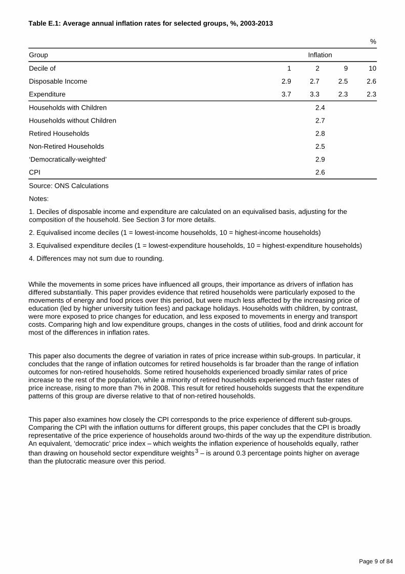
Households without children and retired households have also experienced a faster rate of price increase than households with children and non-retired households respectively – although both these differences are an order of magnitude smaller than the differences between households with different levels of expenditure. Supporting analysis suggests that housing costs have also played an important role: groups with a greater incidence of mortgaged owner-occupiers have enjoyed lower rates of price increase over this period as a consequence of lower mortgage interest payments. These results are summarised in Table E.1 below:
Page 9 of 84
Table E.1: Average annual inflation rates for selected groups, %, 2003-2013
%
Group Inflation
Decile of 1 2 9 10
Disposable Income 2.9 2.7 2.5 2.6
Expenditure 3.7 3.3 2.3 2.3
Households with Children 2.4
Households without Children 2.7
Retired Households 2.8
Non-Retired Households 2.5
‘Democratically-weighted’ 2.9
CPI 2.6
Source: ONS Calculations
Notes:
1. Deciles of disposable income and expenditure are calculated on an equivalised basis, adjusting for the composition of the household. See Section 3 for more details.
2. Equivalised income deciles (1 = lowest-income households, 10 = highest-income households)
3. Equivalised expenditure deciles (1 = lowest-expenditure households, 10 = highest-expenditure households)
4. Differences may not sum due to rounding.
While the movements in some prices have influenced all groups, their importance as drivers of inflation has differed substantially. This paper provides evidence that retired households were particularly exposed to the movements of energy and food prices over this period, but were much less affected by the increasing price of education (led by higher university tuition fees) and package holidays. Households with children, by contrast, were more exposed to price changes for education, and less exposed to movements in energy and transport costs. Comparing high and low expenditure groups, changes in the costs of utilities, food and drink account for most of the differences in inflation rates.
This paper also documents the degree of variation in rates of price increase within sub-groups. In particular, it concludes that the range of inflation outcomes for retired households is far broader than the range of inflation outcomes for non-retired households. Some retired households experienced broadly similar rates of price increase to the rest of the population, while a minority of retired households experienced much faster rates of price increase, rising to more than 7% in 2008. This result for retired households suggests that the expenditure patterns of this group are diverse relative to that of non-retired households.
This paper also examines how closely the CPI corresponds to the price experience of different sub-groups. Comparing the CPI with the inflation outturns for different groups, this paper concludes that the CPI is broadly representative of the price experience of households around two-thirds of the way up the expenditure distribution. An equivalent, ‘democratic’ price index – which weights the inflation experience of households equally, rather than drawing on household sector expenditure weights – is around 0.3 percentage points higher on average 3
than the plutocratic measure over this period.

Page 10 of 84
Next release: To be announced
Release date: 15 December 2014
Contact: Philip [email protected]
1.
2.
3.
1.
Our findings have several implications, of which two are particularly clear. First, it is apparent that while the CPI captures movements in prices for the household sector as a whole, the degree of variation in the price experience of different households is relatively broad. Rates of price increase vary systematically across household types and composition, to differing degrees in different periods. That degree of variation needs consideration alongside movements in the headline rate of CPI inflation. A first step towards greater understanding and appreciation of these differences could be for a distributional analysis of inflation trends to be published on a regular basis. In line with our findings, this could incorporate estimates of within-group inflation differentials, as well as between group differences. This would allow these differentials to be monitored through time, to see whether the trends observed during this period are sustained as the economy continues to recover.
Secondly, the degree of variation presented here has broader implications for economic policy. In particular, it suggests that some sub-groups of the UK population have faced relatively strong headwinds in recent years, eroding both their real incomes and their capacity to spend. The results also suggest that when inflation is relatively high, the dispersion of inflation outcomes is relatively broad. As a consequence, the strength of price growth during the recent economic downturn resulted in a broadening of inflation outcomes among different household types. Both effects suggest that distributional analysis of this nature can offer significant insights on current macroeconomic developments.
Finally, we present a range of avenues for further study, developing on the methods we have employed here. First, future research could seek to quantify the extent to which different households face different prices for the same product. In common with previous studies, this paper assumes that all households face the same prices and as a consequence, inflation differentials are driven by expenditure shares alone. If different households face different prices for the same products, and if these prices grow at different rates, then their experience of inflation may differ from the estimates presented here. Secondly, further work could be carried out to extend our findings from CPI to CPIH – allowing housing costs for all households to be included in the sub-group inflation estimates.
Notes for executive summary
Note that households are likely to move between expenditure and income deciles through time, as their economic circumstances change. As a result, the number of households who consistently feature in a single decile may vary.
This measure is less affected by unusually low- or high-expenditure households who appear in our underlying data. 1 = lowest spending decile, 10 = highest spending decile.
See Sections 2 and 7 for more detail.
3. Background notes
Details of the policy governing the release of new data are available by visiting www.statisticsauthority.gov. or from the Media Relations Office email: uk/assessment/code-of-practice/index.html media.relations@ons.
gsi.gov.uk
Compendium
Methods, data and literature

Page 11 of 84
Table of contents
1. Section 2. Theory
2. Section 3. Data & methods
3. Section 4. Context & literature
4. Background notes

Page 12 of 84
1 . Section 2. Theory
A price index has two basic ingredients: data on the quantity of products purchased and information about the prices of those products. These two ingredients may be combined in various ways to produce different forms of price index: in the UK, the Consumer Prices Index (CPI) uses a Lowe price index, which is a Laspeyres-type index. This uses expenditure data from the previous period alongside information on prices in this and previous 1
periods, and is shown in equation [2.1]:
Equation 2.1
where I is the index value, p is the price level, q is the volume purchased and r, t and i index the reference period, time and items respectively. In more simple terms, this formulation involves using changes in prices alongside expenditure weights from a fixed period. The prices of items that account for a larger (smaller) fraction of expenditure in the reference period are given a greater (lesser) weight in the calculation of the overall index. From this perspective, the formulation of a price index for a subset of households is trivial. For a subset of households, A, the price index equivalent to [2.1] is calculated using data on the expenditure of those households and the prices which they face:
Equation 2.2
By extension, the equivalent price index for any given household, a, is given by [2.3]:
Equation 2.3
Equations [2.1] to [2.3] therefore set out the information that is needed to calculate price indices for all households, a subset of households and an individual household respectively. However, equations [2.2] and [2.3] also have the property that they if they are weighted to reflect the spending of the relevant unit, the all-household price index can be recovered:
Equation 2.4

Page 13 of 84
where e and E are unit and whole-economy household expenditure respectively. This formulation highlights a further feature of these price indices that is relevant for this analysis. Equation [2.4] shows that the standard Laspeyres-type price index used in the CPI weights the price experience of different households by their share of expenditure. While this is not an explicit design of the methodology – which more heavily weights the prices of high-expenditure items – a corollary of this approach is that households that spend more each period have a greater weight in the calculation of the CPI than households who spend less .2
This can lead the price experience of a subset of households to differ from the published CPI – in particular among those households whose expenditure patterns differ substantially from that of the average for the sector as a whole. Price indices of this form are described as having ‘plutocratic weights’, and have the feature that they more heavily weight high-spending households. However, while this is standard international practice, alternative weighting mechanisms can be deployed.
One potentially interesting alternative formulation is a so-called ‘democratic ’ price index, which is shown in 3
equation [2.5], where n represents the number of households:
Equation 2.5
In this formulation, each household receives an equal weight, regardless of their level of spending. The aggregate democratic price index consequently takes the average of the values for each household. In the absence of longitudinal data, this form of price index uses expenditure weights calculated by simply averaging the weight assigned to each product across households.
Note that the level of aggregation in [2.5] is crucial: taking price indices at anything above the household-level (which would implicitly require weighting of some form), would place different weights on different households. As a result, a democratic index is a relatively data-intensive form of price index, requiring household-level expenditure and price information. In general, the difference between the plutocratic and democratic indices will be larger (smaller) when the composition of household spending varies considerably (very little) across households.
Notes for Section 2. Theory:
Page 14 of 84
1.
2.
3.
The CPI is a Lowe index, in the sense that it uses current-period price information alongside expenditure weights that are price-updated. This latter feature distinguishes it from a Laspeyres price index, which uses current period price information with observed, previous period expenditure weights. For notational simplicity, we present these price-updated weights as if they were observed and, as a consequence, our treatment here appears more like a Laspeyres index. See Appendix A.
To see this, consider an economy with two households: one high-spending and one low spending household. Suppose that the majority of the high spending household purchases are devoted to high-inflation products, while the majority of the low-spending household purchases are devoted to low-inflation products. The CPI for this economy – which uses the total amount of household spending – will more closely reflect the inflation experience of the high-spending household, as the weights for the sector as a whole are closer to its expenditure shares than the low-spending household. As a result, the CPI will be above the inflation rate experienced by the low-spending household, and close to (although below) the inflation experience of the high-spending household. The degree of the inflation differential will vary depending on the extent to which household spending shares differ.
Note that the naming convention here can be misleading: In a ‘democratic’ index, each household is given an equal weight, rather than each individual, which might be implied from its name. A ‘truly’ democratic index would weight each person in an economy equally, and would deviate from the popular convention of a ‘democratic’ index to the extent of variation in household size. Arguably, a still ‘truer’ index would use longitudinal data to observe movements in expenditure patterns for the same individuals through time; however, this approach is data-intensive, challenging to implement, and its interpretation not straightforward.
2 . Section 3. Data & methods
3.1 Data
As set out in Section 2, price indices have two ingredients: data on expenditure by product and information about prices for each of these products. This section sets out the data used in this paper to calculate aggregate, decile and sub-group price indices and rates of inflation.
3.1.1 Price data
The price data that are used in this paper are taken from the Consumer Prices Index (CPI). The CPI is calculated from around 100,000 price quotes taken every month for a range of products in different shop types across the regions and nations of the UK. These are supplemented by a centralised collection of a further 80,000 monthly price quotes, ensuring that the CPI is based on around 180,000 price quotes for around 700 goods and services each month. These price quotes are weighted using expenditure data from the National Accounts to ensure that the basket of goods and services reflects the spending of the household sector as a whole (ONS, 2014a).
As household-level expenditure data for individual products can be volatile and intractable, this analysis uses expenditure and price data that is aggregated to the 85 class-level categories defined in the Classification of Individual Consumption According to Purpose (COICOP) (UNSD, 2014) . This detailed dataset therefore provides 1
information about how prices have evolved for 85 groups of goods and services, ranging from bread & cereal to pharmaceutical products, from health insurance to air travel products. These indices are used in their unrounded format, as they are produced prior to the publication process to ensure that errors arising from data aggregation are minimised.

Page 15 of 84
Figure 3.1 shows price indices for several COICOP class-level categories that sit within the ‘food’ group for the 2002 to October 2014 period. It highlights five specific class-level price indices, as well as the weighted movement for the entire group (the dashed line) and summarises the movement of the remaining four price indices in this group using a swathe to denote the range. Figure 3.1 gives some idea of the detail of the categories on which this analysis is based, and demonstrates that there can be substantial differences in price movements across different COICOP classes. For instance, the prices of sugar products & confectionary grew by 65.6% over this period, compared with 43.0% and 43.6% for fruit products and meat products respectively .2
Figure 3.1: Class-level price indices for 1.1: Food, 2002=100
Source: Office for National Statistics
However, the use of these data introduces the first of several limitations into our analysis. As shown in equation [2.3] above, the calculation of ‘true’ sub-group specific price indices requires the use of household-specific prices. However, as price data are collected from retailers rather than by asking households which prices they face, separate price indices are not available for different types of household. As a result and in common with previous, similar studies, this analysis assumes that households all face the same class-level CPI average prices. This limitation is discussed in greater detail in Section 8.

Page 16 of 84
3.1.2 Expenditure data
The expenditure data used in this analysis come from several different sources. First, household-level expenditure data are taken from the Living Costs and Food Survey (LCF). This continuous, cross-sectional survey gathers detailed expenditure data from between 5,500 and 6,500 households per year through a structured interview and an expenditure diary. A range of data, including the size and composition of the household, the household’s tenure, the level of any mortgage interest payments and household income are also gathered, alongside the components required to calculate household-level expenditure for each of the 85 COICOP class-level categories. As a consequence, it allows a more detailed examination of spending by different household types than any other expenditure survey carried out by ONS.
The underlying LCF household-level sample consists of 73,506 households, surveyed between Q1 2002 and Q4 2013. A preliminary analysis of this sample suggested that there were a small number of households whose expenditure we regarded as implausibly concentrated on a single product type. We dropped 125 households (0.17% of the sample) on the basis that 80% or more of their total expenditure was concentrated in a single COICOP category. Secondly, we dropped a further 600 households (0.82% of the sample) who reported negative spending on any COICOP class – possibly reflecting the un-winding of prior overpayment. Taken together, these exclusions amount to 0.99% of the starting sample, and have no discernible impact on our results.
In addition to micro-level data from the LCF, this analysis also makes use of the aggregate household spending data which underpin the weights used in the construction of the CPI. Using these data allows us to (a) replicate the CPI directly; (b) calculate the difference between the published index and the price experience of households; and (c) analyse the impact of different weighting structures on price outcomes. These data were provided to us as annual expenditure totals, which we aggregated to expenditure totals for the class-level of COICOP.
How and why do the weights from the LCF and the CPI differ? Figure 3.2 shows a simplified process map for the calculation of CPI weights. While the LCF weights – as published in the ‘Family Spending’ release (ONS, 2014c) – are an input for the National Accounts and therefore for the CPI weights, it is only one of a number of sources used to estimate household expenditure. Alternative sources are used where the LCF is believed to under-report expenditure (including Alcohol and Tobacco) (ONS, 2012), where data quality is deemed to be stronger from administrative sources (including Energy) (ONS, 2014d), or where the concepts captured in the National Accounts differ from the pure expenditure estimates collected in the LCF (ONS, 2014a). This third case applies in particular to the costs of insurance (which are collected on a gross payments basis in the LCF, but on a net payments basis – after insurance payouts – in the National Accounts), used car purchases (collected on a gross expenditure basis, but measured as net household acquisitions in the National Accounts (ONS, 2014e) and estimates of the costs of financial services.
Figure 3.2: Input data for the calculation of the CPI weights

Page 17 of 84
1.
Notes:
Figure shows a number of the sources and processes used in the compilation of the CPI. LCF is the Living Costs and Food Survey, HMRC is Her Majesty’s Revenue and Customs, DECC is the Department of Energy and Climate Change, OfWat is the water regulator, DCLG is the Department for Communities and Local Government, Int. Passenger Survey is the International Passenger Survey.
Secondly, expenditure totals from the LCF and the National Accounts may differ for a range of data processing reasons (shown in blue in Figure 3.2). Estimates of expenditure from the LCF may be affected by the GDP balancing process before they are used to calculate the weights for CPI. Additional adjustments are made to account for the spending of households from overseas in the UK. Further differences also arise because of issues of timing: to calculate current-year CPI expenditure weights each January (when LCF data for the current year is not yet available), observed expenditure from a previous year is ‘price updated’ (see Appendix A). This involves taking the expenditure totals in this previous year and imputing their current value using recent price changes. All of these practices are common across countries, but result in differences between the equivalent CPI and LCF estimates of household spending, shown for the 20 highest class-level expenditure categories in the LCF in Figure 3.3.
Figure 3.3: Difference between CPI and LCF expenditure totals in selected COICOP classes, %, 2011
Source: ONS Calculations
Notes:

Page 18 of 84
1. This figure shows the difference between total LCF and CPI expenditure as a fraction of LCF expenditure for each product type in 2011. Bars to the right (left) of the axis indicate that the expenditure total is larger (smaller) in the CPI.
As the preceding discussion implies, Figure 3.3 suggests that the differences between the LCF and CPI weights are largest where alternative sources are used, or where the measurement concepts differ between the CPI and LCF. Household spending on gas is higher in the CPI than in the LCF as expenditure in the former is based on information from the Department for Energy and Climate Change, which is notably higher than the LCF estimates. Equally, the weight accorded to transport insurance in the LCF – which captures the cost of insurance premiums – is notably lower than the CPI estimate – which captures the cost of premiums less any claims.
A more detailed discussion of these differences and their impact on this analysis is deferred to the following section. However, it is worth noting at this point that a natural consequence of this discussion is that a price index based on LCF expenditure weights alone will not recover the CPI rate of inflation. Only when these alternative data sources are used and measurement concepts aligned are the CPI weights and inflation rate recoverable.
3.2 Methodology
The methods used in this analysis mirror those used in the calculation of the CPI. Unrounded class-level price indices for each month are taken from the CPI and placed alongside appropriate expenditure weights to produce an aggregate price index. The resulting indices are double chain-linked; first in January, which accounts for the annual changes in the COICOP weights for the class-, group- and division-level products (as set out in Appendix B). A further chaining step, to account for changes in the basket of representative items – the goods and services that are aggregated up to form the class-level of CPI – occurs in February . To calculate the annual inflation 3
rates, the monthly observations for each group are averaged across the year, and rates of change are estimated .4
As a result, the only singular element of this work is in the construction of the expenditure weights, for which there are several candidate sources of data. To ensure the robustness of our analysis and to present interesting differences between measures, this paper replicates all of its results using three different sets of household spending data. The differences between the three resulting sets of expenditure weights are set out below. In the results that follow in Section 5, we focus on the third of these datasets. Section 6 uses the second dataset to assess the inclusion of housing costs on inflation rates. The full results using each set of weights are available in the Reference Tables.
Dataset 1: Weighted expenditure from the LCF
Dataset 1: Weighted expenditure from the LCF (74.5 Kb Excel sheet)
The first set of expenditure weights used in this analysis is the most straightforward. Using the micro-level data from the LCF, we calculate estimates of spending in each of the 85 class-level COICOP categories for each surveyed household. These totals are weighted to reflect the population as a whole and then aggregated across various sub-groups to yield sub-group specific expenditure weights. More explicitly, we aggregate these household-level weighted expenditure totals into: (a) equivalised disposable income deciles; (b) equivalised 5
expenditure deciles; (c) households with and without children; and (d) retired and non-retired households . This is 6
repeated for each year of our data, yielding expenditure weights for each sub-group in each period. These weights are used alongside the class-level COICOP price indices from the CPI. The resulting series are aggregated using the same process as for the CPI and then averaged across the year.7
Dataset 2: Weighted expenditure from the LCF and Mortgage Interest Payments
Dataset 2: Weighted expenditure from the LCF and Mortgage Interest Payments (74.5 Kb Excel sheet)
Page 19 of 84
While the 85 class-level categories of COICOP include a range of different types of expenditure, they exclude any costs associated with the owner occupation of dwellings. Changes in rental costs, by contrast, are used in the CPI and are included in the 85 class-level categories. While the precise mechanism by which housing costs are included in price indices is a matter of some debate (ILO, 2004), the inclusion of housing costs for some of the population (those who rent) and not for others (home-owners with mortgages or owner occupiers) is a short-coming of our work, in particular as different forms of tenure will be more prevalent in some sub-groups than others.
In the context of our work, there are several different ways that housing costs for non-renters could be incorporated, some more difficult than others. In particular, perhaps the most attractive avenue is to produce a measure of sub-group inflation consistent with CPIH, including changes in the cost of owner occupation through the calculation of rental equivalence (ONS, 2014a). However, the production of micro-level estimates of rental equivalence is highly data intensive, requiring a complex array of data on different forms of tenure, housing and geographical area. This has been left for future work.
However, the costs of owner occupation – and in particular the costs associated with mortgage repayments – are often non-trivial fractions of household budgets. As a consequence, we create a second dataset, in which the 85 COICOP categories from the LCF are supplemented by interest payments on mortgages (excluding capital repayments). The resulting weights are used alongside the same CPI price indices as above, as well as the mortgage interest price index from the Retail Prices Index. While we recognise that this is a partial measure of housing costs – and in particular fails to capture the costs associated with owner occupation for households who do not have mortgages – it does allow us to consider a broader measure of housing costs than in Dataset 1. It is also worth noting that the treatment of insurance and the purchase of second hand vehicles remains on the ‘gross’ basis here – excluding the value of any claims or inter-household transfers respectively.
Dataset 3: Reconciling National Accounts totals with the LCF micro-data
Dataset 3: Reconciling National Accounts totals with the LCF micro-data (74.5 Kb Excel sheet)
The third expenditure dataset – on which the majority of the analysis in this paper is based – involves a micro-level reconciliation of the LCF and CPI expenditure weights, which differ for a range of reasons (see Section 3.1). This dataset – which represents one of this paper’s primary contributions to the literature – is composed of household-level expenditure estimates which aggregate to the CPI expenditure weights.
In order to produce a dataset of household-level spending estimates that is consistent with the CPI, this paper makes a series of assumptions designed to allocate the CPI expenditure total across the observed LCF households. In principle, there are several different ways that this could be achieved. Under our method, we seek to impose as few assumptions as possible on the data, and consequently employ a relatively simple rule which divides reported total CPI expenditure on each COICOP class among the households we observe in the LCF in proportion to their observed spending on that class-level category:
Equation 3.1

Page 20 of 84
where e is the level of expenditure consistent either with the CPI or LCF and where a, i and t index households, COICOP classes and time respectively. More simply, equation [3.1] states that total CPI-consistent spending on a given product is divided among the observed households in proportion to the share of total observed spending on that product reported in the LCF. Households that report more (less) expenditure on a given product are awarded a greater (lesser) fraction of total expenditure taken from the CPI. For instance, if an observed household 8
accounts for 0.05% of total purchases of bread & cereal products in the LCF, it is allocated the same fraction of the CPI expenditure total on bread & cereal. This simple attribution mechanism is a second limitation of our analysis – discussed in greater detail in Section 8 – and requires an important assumption: that where there are differences between the LCF and National Accounts totals for a given COICOP, these difference arise because all households over- or under-report their expenditure by the same proportion.
Extending the dataset to 2014
While the CPI weights and price indices that are used in this paper are available from December 2000 to October 2014, the LCF expenditure data that we use is only available on a comparable basis for the period 2002 to 2013. To extend our work to the most recent data, we price update the expenditure weights for individual households observed in 2013 to yield an imputed household-level dataset for 2014. The aggregate CPI weight for 2014 is consequently distributed among these imputed households in a manner discussed above, and in greater length in Section 8. This approach is consistent with the calculation of the weights for the CPI itself, and will only affect our results if different sub-groups experience stronger or weaker substitution effects (Levell and Oldfield, 2011). This assumption adds a further 5,117 imputed household observations to our dataset, resulting in a total sample size of 77,898 across the 2002 to 2014 period. Finally, note that while this approach allows us to extend our analysis by equivalised expenditure deciles and household types to 2014, the income data required to complete an analysis by income decile only extends to 2013. Consequently, our analysis presents inflation rates for the former groups of households to 2014, but only to 2013 for households in different income deciles.
Notes for Section 3. Data & methods
Page 21 of 84
1.
2.
3.
4.
5.
6.
7.
8.
See Appendix B for more information
These differences make a strong case for using more disaggregated expenditure to analyse sub-group specific inflation rates: higher level price indices will only reflect the price experience of sub-groups if all households purchase the group’s class-level components in equal proportions. Further discussion of the appropriate level of aggregation is deferred to the following section and Section 8.
Further technical information on how the CPI is constructed is available in the CPI Technical Manual (ONS, 2014a), while a higher level summary is available as an infographic (ONS, 2014f).
When presenting annual inflation rates in the following tables and figures, this paper does not include data for 2014 as price data is only available up to October 2014.
The ‘equivalisation’ process adjusts household specific expenditure and income to take account of household composition and is based on the OECD-modified scale equivalisation factors used in the ONS publication on the Effects of Taxes and Benefits (ONS, 2014b). Conceptually, this process accounts for the fact that households with more members are likely to need a higher income to achieve the same standard of living as households with fewer members. However, while a household with two people in it will need more money to sustain the same living standards as one with a single person, the two person household is unlikely to need double the income. It is on this basis that households are divided into deciles for distributional analysis.
The respective sub-sections in Section 5 contain the relevant definitions for these sub-groups.
In particular, the resulting series are double-chain linked – once in January (to reflect changes in the expenditure weights) and once in February (to reflect changes in the products included in the CPI) (ONS, 2014a).
To be precise, we weight household spending from the LCF, and calculate the share of weighted expenditure accounted for by each observed household. This fraction of the CPI expenditure total is allocated to that household. Note that this implicitly means that this dataset adopts the concepts and expenditure definitions of the CPI.
3 . Section 4. Context & literature
A wide range of papers have calculated price indices and inflation rates for population sub-groups in a variety of countries for different time periods. This section first examines the papers that consider the UK evidence, before turning to inflation estimates from a range of other countries.
4.1 UK studies
One of the earliest UK papers to calculate sub-group price indices is Crawford (1994). Looking at the period 1979 to 1992, he found a maximum spread of inflation of 1.6 percentage points between the richest and poorest households. However, while the spread could be high within each year, the differences over the whole period were small. Households in the poorest and richest income groups frequently switched between experiencing the highest and lowest inflation rates and consequently balanced out any within year variation. He concluded that the extent of inflation differences between groups varies depending on the period studied, and on the respective prices of luxuries and essentials and the impact they have on different sub-groups.

Page 22 of 84
The studies that have followed – see, for example; Levell and Oldfield (2011), Pike et al., (2008), Crawford and Smith (2002), Adams et al., (2014) – have all reached similar conclusions. The various periods that have been studied have seen different sub-groups of the population experience different rates of inflation. In particular, Crawford and Smith (2002) found statistically significant differences in average inflation rates experienced by income deciles in most of the 25 years studied, with a maximum spread of around 2 percentage points. However, they conclude that no single group has consistently experienced higher or lower inflation than average. Among these previous studies, analyses that focus on the same period as this work (2003-2014) are particularly relevant. These have concluded that the lower income deciles experienced high inflation rates in years that saw large rises in the price of food and fuel, for example 2006 and 2008 (Levell and Oldfield, 2011).
The Living Cost and Food Survey (LCF) dataset used in this article has been used in various forms in most UK studies looking at sub-group price indices, reflecting the fact that, while there are limitations to this source (see Section 8), it is the most complete dataset that is available to look at spending patterns of UK households. However, the methods used to calculate inflation rates for sub-groups differ from paper to paper. Most previous work uses the observed spending of a given household in the LCF, then ‘price updates’ that expenditure to the next period – effectively calculating the change in the cost of a fixed consumption basket. This individual household inflation rate is then weighted – either ‘plutocratically’ or ‘democratically’ (see Sections 2 and 7) – to produce an aggregate index. However, this method assumes that there is no between-year substitution at the household-level, making it inconsistent with the Consumer Prices Index (CPI), which permits between-year substitution effects (ONS, 2014a). Another method, as presented in Crawford (1994), is to use a Tornqvist index. This form of price index uses expenditure weights from the previous and current periods together to deliver a price index which is more sensitive to substitution effects between years. However, as the LCF is cross-sectional – providing snap-shots of household-level of expenditure in a single period – this approach is less appropriate for our dataset.
Several different sub-groups have been the target of previous analyses. As well as the inflation experience of households in different income deciles discussed above, households with and without children (for example; Crawford, 1994, Crawford and Smith, 2002) and retired and non-retired households (for example; Levell and Oldfield, 2011, Pike et al., 2008, Crawford and Smith, 2002, Leicester et al., 2008) have all been subject to recent work. These studies found that there is no significant difference observed in the inflation experience of households with and without children, with a maximum spread of +/- 0.2 percentage points. Crawford (1994) noted however that the presence of children leads to the household taking on spending patterns similar to that of poorer households: adults forego luxuries and spend more of their budget on goods like food and clothing. By comparison, inflation rates for retired and non-retired households have varied significantly over the last two decades with a maximum spread of just under 3 percentage points. The main drivers behind this spread are rises in food and fuel prices for retired households, and changes in mortgage interest payments for the non-retired households (Leicester et al., 2008).
The conclusions of these papers support the notion that while there are often quite large inflation differentials in specific years, these tend to average out over longer time-frames. Leicester et al. (2008) go further and argue that while inter-sub-group differences are important, intra-group variation is equally substantial. For instance, their analysis – which shows that the various drivers of inflation in recent years has impacted on different types of pensioner households to differing degrees – leads them to the conclusion that it is misleading to talk about a single price index for a sub-group. This thesis is examined more in Section 7.
Finally, a number of previous studies have calculated democratically- and plutocratically-weighted price indices for UK sub-groups and examined the difference between these measures. In particular, Crawford and Smith (2002) found a statistically significant difference between the plutocratic and democratic inflation rates in 18 out of the 25 years studied.
Page 23 of 84
4.2 International studies
The question of different sub-groups of the population facing differing inflation rates was first raised internationally in the late 1950s, when Arrow highlighted the different expenditure patterns of households in the US that lay in different parts of the income distribution, and stated “there should be a separate cost-of-living index number for each income level” (Arrow, 1958). Since then, various studies have been conducted over different time periods and looking at different population sub-groups in various economies. Oosthuizen (2007) presents a summary of international work on sub-group price indices as background for an analysis of inflation experiences in South Africa from 1998 to 2006. This developed earlier work by Ley (2005), which summarised twelve studies examining the inflation rates experienced by different sub-groups from countries such as the US and Argentina. Supporting the findings of recent UK research, both these papers found that no single sub-group consistently experienced a higher or lower inflation rate relative to other groups in the long run. However, within years, there were statistically significant differences experienced by households in different sub-groups.
More recent work includes Hait and Janský (2014) who examined the inflation experiences of households in the Czech Republic in the period 1995 to 2010. They found that only around 60% of households experienced inflation similar to the national average, with higher inflation rates experienced by pensioner households and those with low incomes. This is a theme that runs through much of the literature; households that spend a large proportion of their budget on goods and services that are exposed to large price rises face higher inflation rates. In periods where prices for luxuries are rising at a faster rate than for essentials, this is likely to be high income households, while in periods when the cost of household essentials is rising more quickly, this is likely to be low income and retired households who have limited capacity to substitute towards cheaper products. Much of this work consequently finds that inflation differentials are particularly sensitive to changes in the price of fuel and energy (see, for example, work on US inflation by Hobijn and Lagakos (2005), and work on Austrian inflation by Fritzer and Glatzer (2009)).
In common with this paper, several international studies acknowledge the possibility that differences in sub-group inflation rates could also be caused by price differentials for specific goods across sub-groups. In particular, Oosthuizen (2007) states that “prices are collected from outlets that are generally chosen to be representative of the official population, while this is unlikely to be the case for a specific sub-group”. Ley (2005) outlines how some national statistical offices have looked to overcome this problem. In particular, the Indian Ministry of Statistics and Programme Implementation collect distinctive prices for every sub-group they produce inflation rates for, based on a sample of shops visited by each respective sub-group. Other national statistical offices – see, for example; Australian Bureau of Statistics (2014) and US Bureau of Labor Statistics (2012) – produce sub-group indices based on prices sourced directly from the CPI. However, the Australian Bureau of Statistics make exceptions in cases where it is known that different sub-groups face different prices, such as subsidised public transport fares and pharmaceuticals for retired households.
A number of these international studies also examine the differences between plutocratic and democratic price indices, both for whole economies and for sub-groups within their populations. Oosthuizen (2007) provides a useful summary of the alternative measures, how they differ and in which circumstances each is more appropriate or useful. Most recent papers reference her argument that a plutocratic average is useful for understanding inflationary pressure in the broader economy because the contribution of higher expenditure households is “in line with the overall structure of consumer spending”. By contrast, democratic weights provide a better understanding of the inflation rates faced by different sub-groups, and can be used to capture the ‘average’ household within each sub-group. Most recent studies have therefore gone on to calculate both the plutocratic and democratic measure of inflation and found there are significant differences between them. Ley (2005) concluded the sign and magnitude of this difference varies across country and by year.
Finally, reflecting the variety of the UK literature, a range of different methods has been adopted to calculate inflation rates in studies of other economies. Only one paper (Fritzer and Glatzer, 2009) adopts a comparable approach to that used in this analysis, focussing on inflation rates in Austria. However, after aligning the underlying household expenditure data with the weights for the CPI, their paper excludes the class-level categories which are distorted by this matching technique.

Page 24 of 84
Next release: To be announced
Release date: 15 December 2014
Contact: Philip [email protected]
1.
4. Background notes
Details of the policy governing the release of new data are available by visiting www.statisticsauthority.gov. or from the Media Relations Office email: uk/assessment/code-of-practice/index.html media.relations@ons.
gsi.gov.uk
Compendium
Results
Table of contents
1. Section 5. Results
2. 5.1 Income deciles
3. 5.2 Expenditure deciles
4. 5.3 Households with and without children
5. 5.4 Retired and non-retired households
6. Background notes

Page 25 of 84
1.
1 . Section 5. Results
This section sets out the results of our analysis. It first considers differences in expenditure patterns and inflation rates between households in different equivalised disposable income deciles, before turning to deciles of equivalised expenditure . It follows this analysis by comparing the rates of inflation experienced by households 1
with and without children and retired and non-retired households.
Throughout this section, the analysis is based on a set of expenditure weights that are consistent with the CPI weights, details of which are available in Section 3. This places some limits on our analysis, which are discussed in Section 8, but allows us to draw direct comparisons between our sub-group inflation rates and the headline Consumer Prices Index (CPI) inflation rate.
Notes for section 5. Results:
The ‘equivalisation’ process adjusts household specific expenditure and income to take account of household composition and is based on the OECD-modified scale equivalisation factors used in the ONS publication on the Effects of Taxes and Benefits (ONS 2014b). See Section 3 for more details.
2 . 5.1 Income deciles
5.1.1 Expenditure weights
As set out in Section 3, this paper uses sub-group specific expenditure weights from the Living Costs and Food Survey (LCF) alongside population-level price indices from the CPI. As a result, the only driver of differences between sub-groups is the share of expenditure which they attribute to each product, delineated by the class-level categories for the Classification of Individual Consumption According to Purpose (COICOP). As a starting point, Figure 5.1 divides the household population into income deciles – ten equally-sized groups of households 1
ranked by their equivalised disposable income – and illustrates household spending on each COICOP division as a percentage of total spending. It shows that – with the exception of the lowest-income decile – spending shares evolve quite smoothly over the deciles. Spending on ‘essentials’ such as food, clothing, housing and utilities 2
declines smoothly as a fraction of total spending between deciles 2 and 10; falling from 44.4% of expenditure in the 2nd income decile to just 24.9% in the highest-income households. By contrast, spending on recreation and culture represents 13.2% of the spending in the 2nd income decile, compared with 15.1% for households in the highest-income decile.

Page 26 of 84
Figure 5.1: Expenditure shares by COICOP division, by equivalised disposable income decile; average %, 2002 – 2013
Source: Living Costs and Food Survey, ONS Calculations
The ‘kink’ which is apparent in the expenditure weights between deciles 1 and 2 in Figure 5.1 indicates that the composition of the first decile is slightly unusual. The presence of student households (with low current income, but expectations of higher long-term income) is particularly clear, as the weight accorded to spending on education falls from 3.5% to 0.8% between the 1st and 2nd income deciles, before rising smoothly up to the highest-income groups. Pensioner households – many of whom are ‘income poor, asset rich’, also fall into the first decile. This means that care should be taken when comparing the lowest-income decile to other groups.
5.1.2 Inflation rates
Differences in spending patterns across income deciles cause differences in the inflation experience of these households. Table 5.1 below shows the annual rates of price growth experienced by each equivalised income decile between 2003 and 2013, compared with the CPI annual rate of inflation. The final row of the table shows the average growth rate for each group over the same period. Table 5.1 suggests that there is some variation in the long run in the rate of inflation experienced by households with differing levels of equivalised income: the

Page 27 of 84
average annual rate over this period varies between 2.9% for the lowest-income decile, and 2.4% for the 7th income decile. The CPI – capturing the degree of inflation for all households weighted by their expenditure – sits in the middle of this range, at 2.6%. There is some variation between years: in five out of the eleven years, the lowest-income deciles face the highest price increases but there is no discernible pattern in which households face the lowest inflation rates. These are predominantly found in the 7th and 9th income deciles but in 2010 it is the 4th decile which faces the smallest price increases, and in 2011 it is the 10th decile. Table 5.1 suggests that when the CPI rises, the rate of price increase experienced by each income decile tends to rise as well, limiting the degree of variation in any one period.
Table 5.1: Annual inflation rates for equivalised disposable income deciles, CPI, %
%
Year Equivalised Disposable Income Decile CPI
1 2 3 4 5 6 7 8 9 10
2003 1.5 1.3 1.3 1.5 1 1.2 1.5 1.3 1.3 1.6 1.4
2004 1.3 1.1 1.3 1.2 1.3 1.2 1.4 1.2 1.6 1.4 1.3
2005 2.5 2.9 1.9 1.9 1.9 2.1 1.8 1.9 2 2.2 2.1
2006 2.8 2.6 2.7 2.3 2.3 2.4 2.2 2.2 2.1 2.3 2.3
2007 2.6 2.5 2.5 2.5 2.5 2.2 1.9 2.2 2 2.6 2.3
2008 4.4 4 3.9 4 3.7 3.5 3.1 3.7 3.4 3.4 3.6
2009 2.3 2.4 2.4 2.4 1.9 1.7 2 2.6 2.1 2.1 2.2
2010 3.5 3.1 3.2 2.8 3.4 3.5 3.3 3.6 3.3 3.1 3.3
2011 4.4 4.7 4.3 4.9 4.4 4.2 4.4 4.2 5.1 4.1 4.5
2012 3.3 2.9 2.8 2.6 2.9 2.9 2.5 2.9 2.6 3 2.8
2013 3.5 2.8 2.8 2.6 2.4 2.4 2.4 2.4 2.3 2.6 2.6
Average 2.9 2.7 2.6 2.6 2.5 2.5 2.4 2.6 2.5 2.6 2.6
Source: Office for National Statistics, ONS Calculations
Notes:
1. The average presented is the compound average annual growth rate, and consequently may differ from the arithmetic average of the inflation rates presented.
2. Equivalised income deciles (1 = lowest-income households 10 = highest-income households)
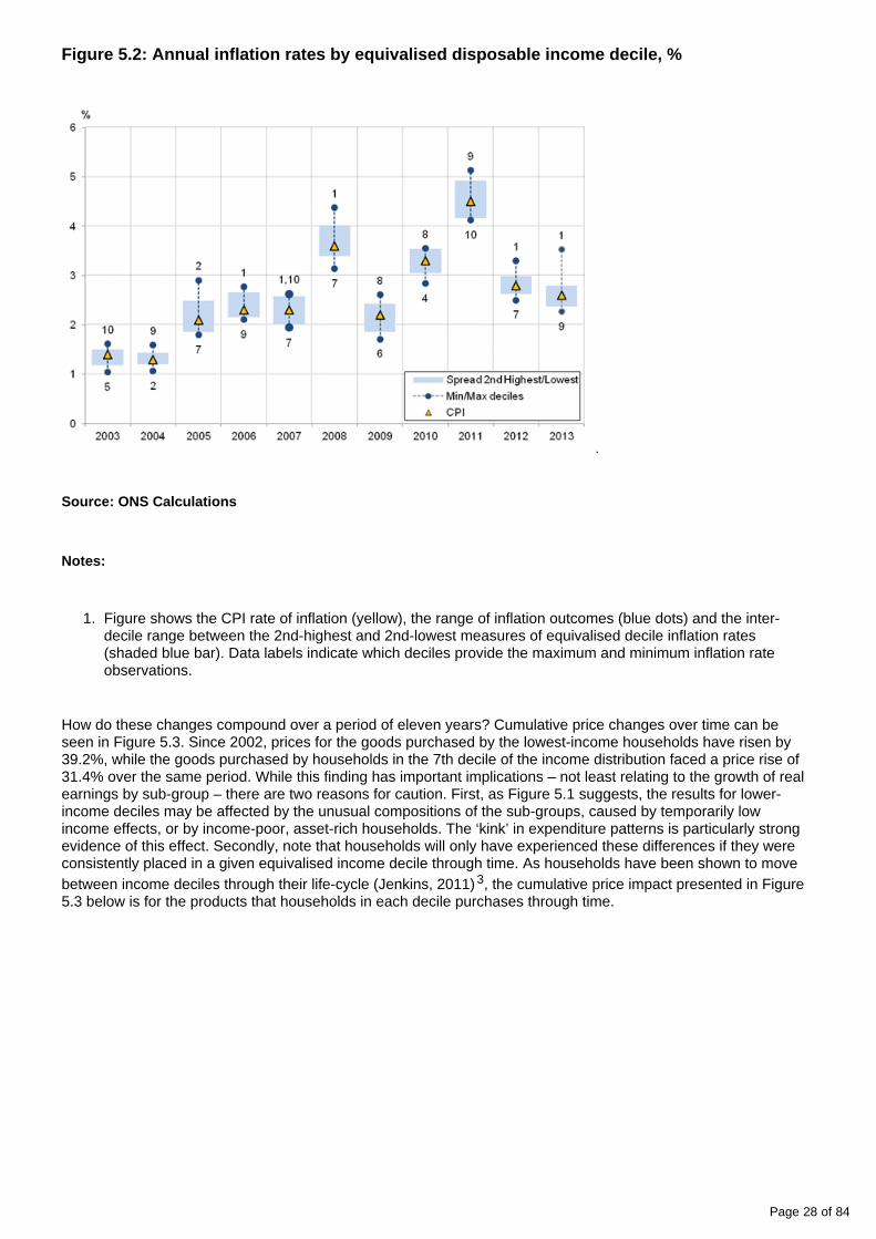
Figure 5.2 below captures this information in a slightly different form. It shows the range of inflation rates experienced each year across the income deciles as blue points connected by the dotted line, as well as the CPI estimate of inflation (yellow triangles). It also shows the inter-decile range between the 2nd-highest and 2nd-lowest measures of inflation as a shaded bar. This measure is less affected by unusually low- or high-income households who appear in our underlying data. At the widest points in 2008 and 2013, the highest and lowest rates of decile-level inflation are around 1.3 percentage points apart, while in 2004, the differences are much smaller. However, the labels on the range of estimates confirm that – in general – it is the lowest-income groups that experience the highest rates of inflation.
Page 28 of 84
1.
Figure 5.2: Annual inflation rates by equivalised disposable income decile, %
Source: ONS Calculations
Notes:
Figure shows the CPI rate of inflation (yellow), the range of inflation outcomes (blue dots) and the inter-decile range between the 2nd-highest and 2nd-lowest measures of equivalised decile inflation rates (shaded blue bar). Data labels indicate which deciles provide the maximum and minimum inflation rate observations.
How do these changes compound over a period of eleven years? Cumulative price changes over time can be seen in Figure 5.3. Since 2002, prices for the goods purchased by the lowest-income households have risen by 39.2%, while the goods purchased by households in the 7th decile of the income distribution faced a price rise of 31.4% over the same period. While this finding has important implications – not least relating to the growth of real earnings by sub-group – there are two reasons for caution. First, as Figure 5.1 suggests, the results for lower-income deciles may be affected by the unusual compositions of the sub-groups, caused by temporarily low income effects, or by income-poor, asset-rich households. The ‘kink’ in expenditure patterns is particularly strong evidence of this effect. Secondly, note that households will only have experienced these differences if they were consistently placed in a given equivalised income decile through time. As households have been shown to move between income deciles through their life-cycle (Jenkins, 2011) , the cumulative price impact presented in Figure 3
5.3 below is for the products that households in each decile purchases through time.

Page 29 of 84
1.
2.
1.
2.
3.
Figure 5.3: Range of cumulative price changes for equivalised disposable income deciles, selected equivalised disposable income deciles and CPI; 2002 = 100
Source: ONS Calculations
Notes:
Equivalised income deciles (1 = lowest-income households, 10 = highest-income households)
Figure shows the range of cumulative price changes for goods purchased by income deciles between 2002 and December 2013. Note that households have been shown to move between deciles between years.
Notes for 5.1 Income deciles
Disposable income is defined as total income less current transfers paid. Such transfers comprise: employers’ social insurance contributions; employees’ social insurance contributions; taxes on income; regular taxes on wealth; regular inter-household cash transfers; and regular cash transfers to charities.
The definition of ‘essentials’ is a matter of extensive debate and research – see, for example; Joseph Rowntree Foundation (2013), and Tullett Prebon (2013). Here, we adopt this label as a matter of convenience, rather than philosophical conviction.
Note that this is a broader issue, which affects a wide range of analyses of distributional outcomes. The ‘axiom of anonymity’ (Grimm, 2005), in which the outcomes for multiple cross sections are analysed without regard to the longitudinal movements within the distribution, may mean that the experience of a given household deviates from the results presented.
3 . 5.2 Expenditure deciles
The weakness of dividing households into equivalised income deciles as shown above is that the composition of at least one group of interest – that of the lowest-income – is affected by its unusual composition. As economists

Page 30 of 84
tend to think that households will smooth consumption through time in the face of income shocks, dividing them into deciles of equivalised expenditure may help to avoid the ‘temporary low income’ or income-poor, asset-rich 1
effects observed above. This section presents the results for deciles of household expenditure.
5.2.1 Expenditure weights
Figure 5.4 shows the share of total expenditure which is allocated to each of the 12 COICOP divisions for each of the equivalised expenditure deciles – ten equally-sized groups of households ranked according to their equivalised expenditure totals. As before, the lowest-expenditure group is accorded the lowest decile number, and the highest-expenditure group is accorded the highest number. As in the income analysis, the weight accorded to some products falls over the deciles, while the weight accorded to others rises. In this analysis, the apparent ‘kink’ between deciles 1 and 2 in the income analysis has disappeared – possibly replaced by a ‘kink’ between deciles 9 and 10. This latter group is now more likely to be composed of those households who had unusually high expenditure in the survey period – perhaps because of a single, large purchase . By eliminating 2
one potential source of bias at the lower expenditure and income end, this may introduce a new, different bias at the top of the expenditure distribution. Consequently, in what follows we present the differences between the 2nd and 9th deciles, in an effort to avoid these potential effects.
Figure 5.4: Expenditure shares by COICOP division, by equivalised expenditure decile; average 2002 – 2014, %
Page 31 of 84
1.
Source: Living Costs and Food Survey, ONS Calculations
Notes:
Equivalised expenditure deciles (1 = lowest-expenditure households, 10 = highest-expenditure households)
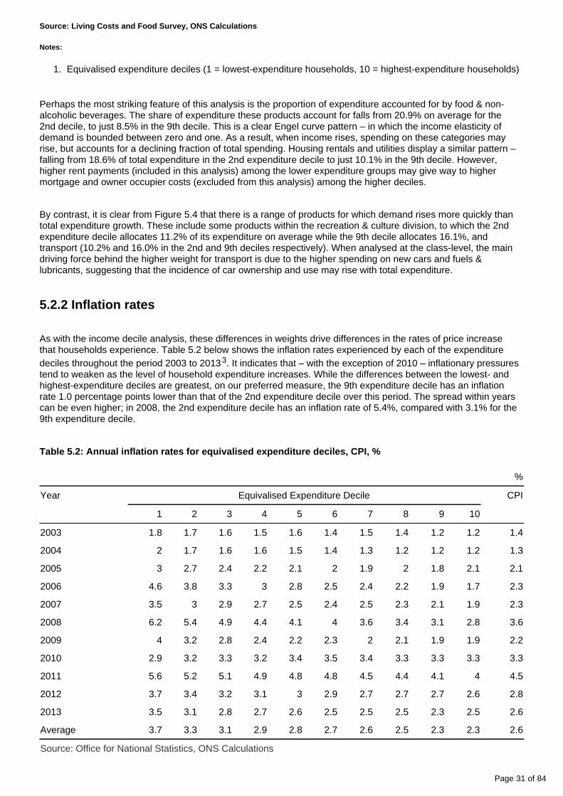
Perhaps the most striking feature of this analysis is the proportion of expenditure accounted for by food & non-alcoholic beverages. The share of expenditure these products account for falls from 20.9% on average for the 2nd decile, to just 8.5% in the 9th decile. This is a clear Engel curve pattern – in which the income elasticity of demand is bounded between zero and one. As a result, when income rises, spending on these categories may rise, but accounts for a declining fraction of total spending. Housing rentals and utilities display a similar pattern – falling from 18.6% of total expenditure in the 2nd expenditure decile to just 10.1% in the 9th decile. However, higher rent payments (included in this analysis) among the lower expenditure groups may give way to higher mortgage and owner occupier costs (excluded from this analysis) among the higher deciles.
By contrast, it is clear from Figure 5.4 that there is a range of products for which demand rises more quickly than total expenditure growth. These include some products within the recreation & culture division, to which the 2nd expenditure decile allocates 11.2% of its expenditure on average while the 9th decile allocates 16.1%, and transport (10.2% and 16.0% in the 2nd and 9th deciles respectively). When analysed at the class-level, the main driving force behind the higher weight for transport is due to the higher spending on new cars and fuels & lubricants, suggesting that the incidence of car ownership and use may rise with total expenditure.
5.2.2 Inflation rates
As with the income decile analysis, these differences in weights drive differences in the rates of price increase that households experience. Table 5.2 below shows the inflation rates experienced by each of the expenditure deciles throughout the period 2003 to 2013 . It indicates that – with the exception of 2010 – inflationary pressures 3
tend to weaken as the level of household expenditure increases. While the differences between the lowest- and highest-expenditure deciles are greatest, on our preferred measure, the 9th expenditure decile has an inflation rate 1.0 percentage points lower than that of the 2nd expenditure decile over this period. The spread within years can be even higher; in 2008, the 2nd expenditure decile has an inflation rate of 5.4%, compared with 3.1% for the 9th expenditure decile.
Table 5.2: Annual inflation rates for equivalised expenditure deciles, CPI, %
%
Year Equivalised Expenditure Decile CPI
1 2 3 4 5 6 7 8 9 10
2003 1.8 1.7 1.6 1.5 1.6 1.4 1.5 1.4 1.2 1.2 1.4
2004 2 1.7 1.6 1.6 1.5 1.4 1.3 1.2 1.2 1.2 1.3
2005 3 2.7 2.4 2.2 2.1 2 1.9 2 1.8 2.1 2.1
2006 4.6 3.8 3.3 3 2.8 2.5 2.4 2.2 1.9 1.7 2.3
2007 3.5 3 2.9 2.7 2.5 2.4 2.5 2.3 2.1 1.9 2.3
2008 6.2 5.4 4.9 4.4 4.1 4 3.6 3.4 3.1 2.8 3.6
2009 4 3.2 2.8 2.4 2.2 2.3 2 2.1 1.9 1.9 2.2
2010 2.9 3.2 3.3 3.2 3.4 3.5 3.4 3.3 3.3 3.3 3.3
2011 5.6 5.2 5.1 4.9 4.8 4.8 4.5 4.4 4.1 4 4.5
2012 3.7 3.4 3.2 3.1 3 2.9 2.7 2.7 2.7 2.6 2.8
2013 3.5 3.1 2.8 2.7 2.6 2.5 2.5 2.5 2.3 2.5 2.6
Average 3.7 3.3 3.1 2.9 2.8 2.7 2.6 2.5 2.3 2.3 2.6
Source: Office for National Statistics, ONS Calculations

Page 32 of 84
1.
Notes:
1. The average presented is the compound average annual growth rate, and consequently may differ from the arithmetic average of the inflation rates presented.
2. Equivalised income deciles (1 = lowest-income households 10 = highest-income households)
Figure 5.5 below presents the equivalent picture for expenditure deciles as Figure 5.2 does for income deciles. The broader range of inflation outcomes on this measure is obvious, with greater dispersion in years when the average level of inflation is high . CPI – again shown as a yellow triangle – remains within the range of decile-4
level outcomes – shown by the blue dots and the shaded bars, which represents the inter-decile range between the 2nd-highest and 2nd-lowest measures of equivalised decile inflation rates. However, in comparison with the income decile results, the degree of variation now implies that some households have experienced very different rates of inflation to that presented in the headline rate. The lowest expenditure decile experiences the highest inflation rate in ten of the eleven years presented, while the highest expenditure decile experiences the lowest rate in all but three.
Figure 5.5: Annual inflation rates by equivalised expenditure decile, %
Source: ONS Calculations
Notes:
Figure shows the CPI rate of inflation (yellow triangle), the range of inflation outcomes (blue dots) and the inter-decile range between the 2nd-highest and 2nd-lowest measures of equivalised decile inflation rates (shaded blue bar). Data labels indicate which deciles provide the maximum and minimum inflation rate observations.
The cumulative effect of these differences is presented in Figure 5.6. It suggests that since 2002, the goods purchased by the highest-expenditure decile have seen prices increase by a total of 31.0%, while the lowest-

Page 33 of 84
1.
2.
expenditure decile experienced price growth of 51.7%. On our preferred, narrower measure, prices have risen by 45.5% for the goods purchased by the 2nd decile, compared with 31.2% for the 9th decile. Following the predictions of Section 2 above, the published CPI inflation figure, which saw a rise of 34.7% between 2002 and October 2014, is more in line with the experience of the higher expenditure deciles . While this finding has 5
important implications, note that households will only have experienced these cumulative differences if they were consistently placed in a given equivalised expenditure decile through time.
Figure 5.6: Range of cumulative price changes for equivalised expenditure deciles, selected equivalised expenditure deciles and CPI; 2002 = 100
Source: ONS Calculations
Notes:
Equivalised expenditure deciles (1 = lowest-expenditure households, 10 = highest-expenditure households)
Figure shows the range of cumulative price changes of products purchased by the respective expenditure deciles between 2002 and October 2014. Note that households may move between deciles between years.
To identify why lower expenditure groups have experienced amongst the highest rates of inflation in recent years, it is necessary to examine the contribution of different types of product to the inflation rate for each decile. Figure 5.7 below is therefore divided into three panels: Panels A and B show contributions to the annual rate of inflation experienced by the 2nd and 9th expenditure deciles respectively, while Panel C shows the difference in these contributions: capturing precisely how these different categories generate inflation differentials.

Page 34 of 84
1.
2.
3.
Figure 5.7A: Contributions to annual inflation experienced by equivalised expenditure decile 2: % and percentage points
Source: INS Calculations
Notes:
Stacked bars reflect the percentage point contributions of each of the 85 class-level items in the Classification of Individual Consumption by Purpose (COICOP) to the annual percentage change in the CPI-consistent inflation rate. The contribution of each of the 85 class-level items is estimated separately, before being aggregated to the categories above. Note that a reduction in the contribution of series to the annual rate of change need not imply falling prices, but could also reflect a lower rate of increase.
Food, drink & tobacco is composed of food, non-alcoholic and alcoholic beverages and tobacco. Housing is composed of actual rents and products and services for the repair of dwellings. Elect., gas & fuel includes electricity, gas and other household fuels as well as fuels and lubricants for motor vehicles. Transport & package holidays includes passenger transport by road, rail, air and sea, as well as package holidays. Education reflects the division-level contribution. The ‘other’ category reflects the combined contributions of the remaining 56 class-level items, bringing the sum of contributions to the inflation rate.
Contributions may not sum due to rounding.

Page 35 of 84
1.
2.
3.
Figure 5.7B: Contributions to annual inflation experienced by equivalised expenditure decile 9: % and percentage points
Source: ONS Calculations
Notes:
Stacked bars reflect the percentage point contributions of each of the 85 class-level items in the Classification of Individual Consumption by Purpose (COICOP) to the annual percentage change in the CPI-consistent inflation rate. The contribution of each of the 85 class-level items is estimated separately, before being aggregated to the categories above. Note that a reduction in the contribution of series to the annual rate of change need not imply falling prices, but could also reflect a lower rate of increase.
Food, drink & tobacco is composed of food, non-alcoholic and alcoholic beverages and tobacco. Housing is composed of actual rents and products and services for the repair of dwellings. Elect., gas & fuel includes electricity, gas and other household fuels as well as fuels and lubricants for motor vehicles. Transport & package holidays includes passenger transport by road, rail, air and sea, as well as package holidays. Education reflects the division-level contribution. The ‘other’ category reflects the combined contributions of the remaining 56 class-level items, bringing the sum of contributions to the inflation rate.
Contributions may not sum due to rounding.
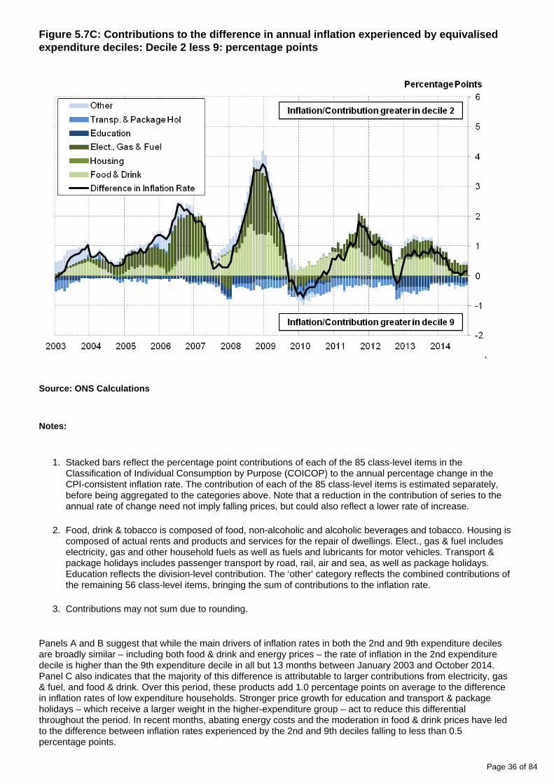
Page 36 of 84
1.
2.
3.
Figure 5.7C: Contributions to the difference in annual inflation experienced by equivalised expenditure deciles: Decile 2 less 9: percentage points
Source: ONS Calculations
Notes:
Stacked bars reflect the percentage point contributions of each of the 85 class-level items in the Classification of Individual Consumption by Purpose (COICOP) to the annual percentage change in the CPI-consistent inflation rate. The contribution of each of the 85 class-level items is estimated separately, before being aggregated to the categories above. Note that a reduction in the contribution of series to the annual rate of change need not imply falling prices, but could also reflect a lower rate of increase.
Food, drink & tobacco is composed of food, non-alcoholic and alcoholic beverages and tobacco. Housing is composed of actual rents and products and services for the repair of dwellings. Elect., gas & fuel includes electricity, gas and other household fuels as well as fuels and lubricants for motor vehicles. Transport & package holidays includes passenger transport by road, rail, air and sea, as well as package holidays. Education reflects the division-level contribution. The ‘other’ category reflects the combined contributions of the remaining 56 class-level items, bringing the sum of contributions to the inflation rate.
Contributions may not sum due to rounding.
Panels A and B suggest that while the main drivers of inflation rates in both the 2nd and 9th expenditure deciles are broadly similar – including both food & drink and energy prices – the rate of inflation in the 2nd expenditure decile is higher than the 9th expenditure decile in all but 13 months between January 2003 and October 2014. Panel C also indicates that the majority of this difference is attributable to larger contributions from electricity, gas & fuel, and food & drink. Over this period, these products add 1.0 percentage points on average to the difference in inflation rates of low expenditure households. Stronger price growth for education and transport & package holidays – which receive a larger weight in the higher-expenditure group – act to reduce this differential throughout the period. In recent months, abating energy costs and the moderation in food & drink prices have led to the difference between inflation rates experienced by the 2nd and 9th deciles falling to less than 0.5 percentage points.

Page 37 of 84
1.
2.
3.
4.
5.
Notes for 5.2 expenditure deciles
For each dataset listed in Section 3.2, equivalised expenditure deciles are created based on the respective total measure of expenditure. In this section, expenditure based on the CPI-consistent weights is used to create the expenditure deciles.
For each household, we calculated the share of expenditure accounted for by the highest-expenditure COICOP class. This share was largest on average in the highest expenditure decile, suggesting that some of the strength of spending in this group is accounted for by large purchases on a single category. Much of this effect is concentrated in miscellaneous goods & services. See Appendix B for more detail.
When presenting annual inflation rates in the following tables and figures, this paper does not include data for 2014 as price data is only available up to October 2014.
This is consistent with work conducted by Crawford and Smith (2002), who found a 1 percentage point increase in the level of inflation led to 0.1 percentage point widening of the inter-quartile range.
This is because the CPI is a plutocratic measure of inflation, and therefore gives a greater weight to households with higher expenditure.
4 . 5.3 Households with and without children
While the income and expenditure characteristics present two methods of grouping households, there is also significant policy interest in differences in the inflation experience of households categorised by other factors. Whether a household contains children is one such dimension, as the goods and services that these households 1
purchase may differ from the purchases of other households.
5.3.1 Expenditure weights
As with the income and expenditure deciles, only differences in expenditure weights can produce inflation rate differentials. Figure 5.8 below shows the weight accorded to each of the COICOP division-level product groups in 2002, 2008 and 2014, by households with and without children. These differ very little through time and between groups, suggesting that at this level of detail, household purchases of the two groups are quite similar. On average, households with children spend more of their budget on education (an average difference of 1.8 percentage points), clothing & footwear (1.6 percentage points) and recreation & culture (1.4 percentage points). These positive weights are offset by a smaller weight on housing & utilities (-2.3 percentage points), reflecting a tendency among these households to use less energy, and for these households to be located in owner-occupied dwellings, rather than rented accommodation (see Section 6).
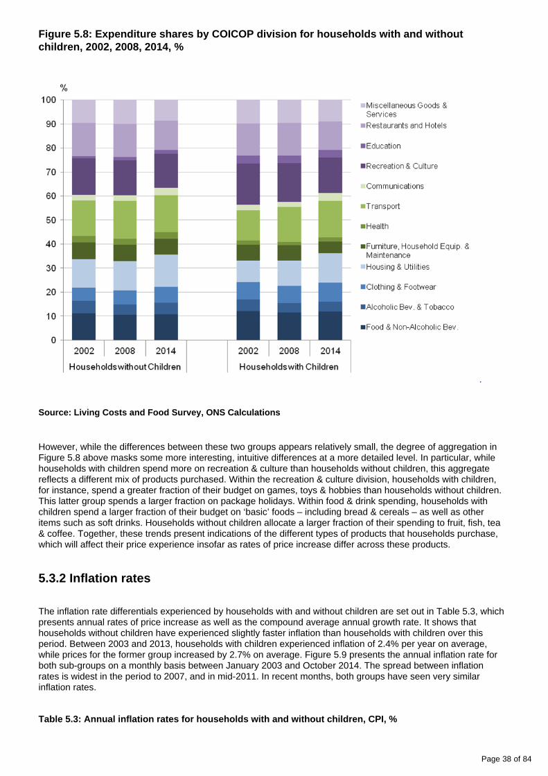
Page 38 of 84
Figure 5.8: Expenditure shares by COICOP division for households with and without children, 2002, 2008, 2014, %
Source: Living Costs and Food Survey, ONS Calculations
However, while the differences between these two groups appears relatively small, the degree of aggregation in Figure 5.8 above masks some more interesting, intuitive differences at a more detailed level. In particular, while households with children spend more on recreation & culture than households without children, this aggregate reflects a different mix of products purchased. Within the recreation & culture division, households with children, for instance, spend a greater fraction of their budget on games, toys & hobbies than households without children. This latter group spends a larger fraction on package holidays. Within food & drink spending, households with children spend a larger fraction of their budget on ‘basic’ foods – including bread & cereals – as well as other items such as soft drinks. Households without children allocate a larger fraction of their spending to fruit, fish, tea & coffee. Together, these trends present indications of the different types of products that households purchase, which will affect their price experience insofar as rates of price increase differ across these products.
5.3.2 Inflation rates
The inflation rate differentials experienced by households with and without children are set out in Table 5.3, which presents annual rates of price increase as well as the compound average annual growth rate. It shows that households without children have experienced slightly faster inflation than households with children over this period. Between 2003 and 2013, households with children experienced inflation of 2.4% per year on average, while prices for the former group increased by 2.7% on average. Figure 5.9 presents the annual inflation rate for both sub-groups on a monthly basis between January 2003 and October 2014. The spread between inflation rates is widest in the period to 2007, and in mid-2011. In recent months, both groups have seen very similar inflation rates.
Table 5.3: Annual inflation rates for households with and without children, CPI, %

Page 39 of 84
%
Households without Children Households with Children CPI
2003 1.5 1.2 1.4
2004 1.4 1.2 1.3
2005 2.3 1.7 2.1
2006 2.4 2.2 2.3
2007 2.4 2.2 2.3
2008 3.7 3.5 3.6
2009 2.2 2.1 2.2
2010 3.3 3.3 3.3
2011 4.7 4.1 4.5
2012 2.9 2.8 2.8
2013 2.5 2.7 2.6
Average 2.7 2.4 2.6
Source: ONS Calculations
Notes:
1. The average presented is the compound average annual growth rate, and consequently may differ from the arithmetic average of the inflation rates presented.
Figure 5.9: Annual inflation rates for households with and without children, CPI, %
Source: ONS Calculations
The cumulative impact of these differences is presented in Figure 5.10 below. Since 2002, prices for households without children have risen by 35.9%, while households with children saw prices rise 32.9% over the same period. As households without children make up a greater proportion of the UK population (in the 2011 Census (ONS 2014g), less than 30% of households included children), the published CPI tracks their inflation experience to a greater extent than that of households with children.
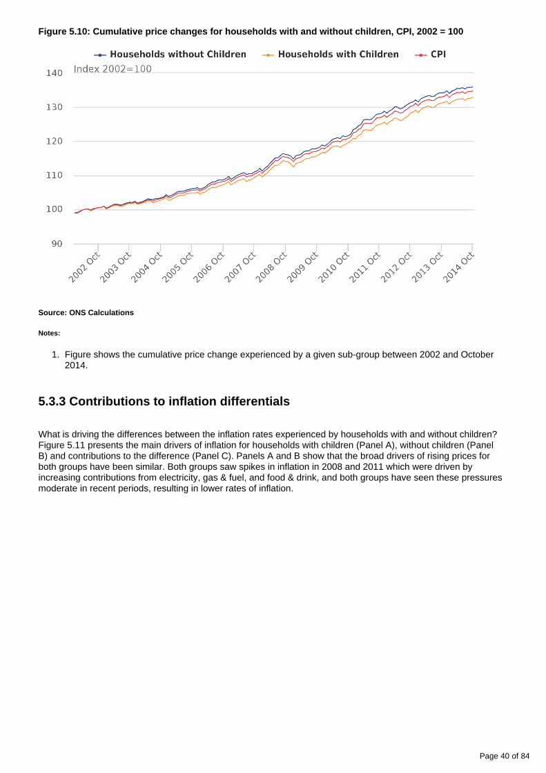
Page 40 of 84
1.
Figure 5.10: Cumulative price changes for households with and without children, CPI, 2002 = 100
Source: ONS Calculations
Notes:
Figure shows the cumulative price change experienced by a given sub-group between 2002 and October 2014.
5.3.3 Contributions to inflation differentials
What is driving the differences between the inflation rates experienced by households with and without children? Figure 5.11 presents the main drivers of inflation for households with children (Panel A), without children (Panel B) and contributions to the difference (Panel C). Panels A and B show that the broad drivers of rising prices for both groups have been similar. Both groups saw spikes in inflation in 2008 and 2011 which were driven by increasing contributions from electricity, gas & fuel, and food & drink, and both groups have seen these pressures moderate in recent periods, resulting in lower rates of inflation.

Page 41 of 84
1.
2.
3.
Figure 5.11A: Contributions to annual inflation experienced by households with children: % and percentage points
Source: ONS Calculations
Notes:
Stacked bars reflect the percentage point contributions of each of the 85 class-level items in the Classification of Individual Consumption by Purpose (COICOP) to the annual percentage change in the CPI-consistent inflation rate. The contribution of each of the 85 class-level items is estimated separately, before being aggregated to the categories above. Note that a reduction in the contribution of series to the annual rate of change need not imply falling prices, but could also reflect a lower rate of increase.
Food, drink & tobacco is composed of food, non-alcoholic and alcoholic beverages and tobacco. Housing is composed of actual rents and products and services for the repair of dwellings. Elect., gas & fuel includes electricity, gas and other household fuels as well as fuels and lubricants for motor vehicles. Transport & package holidays includes passenger transport by road, rail, air and sea, as well as package holidays. Education reflects the division-level contribution. The ‘other’ category reflects the combined contributions of the remaining 56 class-level items, bringing the sum of contributions to the inflation rate.
Contributions may not sum due to rounding.

Page 42 of 84
1.
2.
3.
Figure 5.11B: Contributions to annual inflation experienced by households without children: % and percentage points
Source: ONS Calculations
Notes:
Stacked bars reflect the percentage point contributions of each of the 85 class-level items in the Classification of Individual Consumption by Purpose (COICOP) to the annual percentage change in the CPI-consistent inflation rate. The contribution of each of the 85 class-level items is estimated separately, before being aggregated to the categories above. Note that a reduction in the contribution of series to the annual rate of change need not imply falling prices, but could also reflect a lower rate of increase.
Food, drink & tobacco is composed of food, non-alcoholic and alcoholic beverages and tobacco. Housing is composed of actual rents and products and services for the repair of dwellings. Elect., gas & fuel includes electricity, gas and other household fuels as well as fuels and lubricants for motor vehicles. Transport & package holidays includes passenger transport by road, rail, air and sea, as well as package holidays. Education reflects the division-level contribution. The ‘other’ category reflects the combined contributions of the remaining 56 class-level items, bringing the sum of contributions to the inflation rate.
Contributions may not sum due to rounding.

Page 43 of 84
1.
2.
3.
Figure 5.11C: Contributions to the difference in annual inflation: Households with children less households without children: percentage points
Source: ONS Calculations
Notes:
Stacked bars reflect the percentage point contributions of each of the 85 class-level items in the Classification of Individual Consumption by Purpose (COICOP) to the annual percentage change in the CPI-consistent inflation rate. The contribution of each of the 85 class-level items is estimated separately, before being aggregated to the categories above. Note that a reduction in the contribution of series to the annual rate of change need not imply falling prices, but could also reflect a lower rate of increase.
Food, drink & tobacco is composed of food, non-alcoholic and alcoholic beverages and tobacco. Housing is composed of actual rents and products and services for the repair of dwellings. Elect., gas & fuel includes electricity, gas and other household fuels as well as fuels and lubricants for motor vehicles. Transport & package holidays includes passenger transport by road, rail, air and sea, as well as package holidays. Education reflects the division-level contribution. The ‘other’ category reflects the combined contributions of the remaining 56 class-level items, bringing the sum of contributions to the inflation rate.
Contributions may not sum due to rounding.
Differences between the two inflation rates are more clearly identified in Panel C. In this Panel, positive (negative) bars indicate products that raise (lower) the inflation rate for households with children relative to the inflation rate for households without children. It indicates that housing and utilities (electricity, gas & fuel) have made a negative contribution to the difference – tending to raise the inflation rate of households without children more than the inflation rate of households with children. Contributions from transport & package holidays are volatile, but generally act to reduce the rate of price increase for households with children. The different mix of food products purchased by the two groups has a substantial impact only when the price of food staples increased markedly in 2008, resulting in a larger contribution from these goods to the inflation rate of households with children.

Page 44 of 84
1.
However, perhaps the most striking feature of Panel C is the impact of education, which largely offsets all of the downwards pressures outlined above from housing, utilities and transport. As households with children spend a greater proportion of their expenditure on this group, increases in the cost of schooling and university attendance will affect those households most strongly. The step-changes that are noteworthy in Figure 5.11 occur as a result of the increases in university tuition fees in October 2006 and October 2012 respectively. The latter increase was enough to raise the inflation rate experienced by households with children above that experienced by households without children for the first sustained period in a decade to 2013.
However, while the drivers of price pressure differ between groups, the magnitude of the inflation rate differential between households with and without children is clearly an order of magnitude smaller than that between households at different points in the income and expenditure distribution. Section 7 presents some further evidence which develops this point, highlighting substantial intra-group variation in inflation experiences for both households with and without children over this period.
Notes for 5.3 households with and without children
Households with children are defined here as any household with one or more household members who are under 18 years of age, in full-time education and have never been married.
5 . 5.4 Retired and non-retired households
The rate of price increase experienced by retired or pensioner households has also been of significant policy interest in recent years. Following debate about the extent of increases in the basic state pension, these benefits are now uprated by a ‘triple-lock’, in which the state pension rises by the rate of CPI inflation, the rate of earnings growth or 2.5%, whichever is greatest. This section examines how inflation rates have varied for retired households between 2003 and 2014, while Section 7 examines the distribution of inflation outcomes for retired households in more detail.1
5.4.1 Expenditure weights
The shares of expenditure accorded to broad product groups by retired and non-retired households in 2002, 2008 and 2014 are shown in Figure 5.12. It indicates that the expenditure weights vary quite substantially between these groups. The expenditure share of food & non-alcoholic beverages has been consistently higher for retired than non-retired, although the share for retired households has been converging to the level of non-retired households over time. In 2002 the difference between the expenditure shares was 5.3 percentage points, but by 2014 this has reduced to 2.8 percentage points. Retired households also allocated a greater proportion of their expenditure budget on health (an average gap of 1.9 percentage points) and furniture, household equipment & maintenance (2.1 percentage points). When analysed at a class-level, the increase in proportion of furniture, household equipment & maintenance is related to a higher expenditure share for domestic & household services as well as furniture & furnishings.

Page 45 of 84
Figure 5.12: Expenditure shares by COICOP division for retired and non-retired households; 2002, 2008, and 2014, %
Source: Living Costs and Food Survey, ONS Calculations
By comparison, non-retired households allocate a higher proportion of their expenditure to transport (an average gap of 2.5 percentage points), and in particular to fuels & lubricants – perhaps reflecting the cost pressures that working households face from driving to work. Education (1.8 percentage points) and restaurants & hotels (3.3 percentage points) also receive a higher weight in non-retired households. The gap between restaurants & hotels has slowly been closing over the period, a result of non-retired households allocating a smaller proportion of their expenditure to the class-level restaurants & cafes in recent years – perhaps because of rising cost pressures elsewhere. The lower share of expenditure on education is likely to be a result of the demographic mix of these respective groups.
5.4.2 Inflation rates
Table 5.4 shows the inflation rates experienced by retired and non-retired households over the period 2003-2013, while Figure 5.13 presents this information on a monthly basis between January 2003 and October 2014. Apart from two periods – 2010 and since late 2012 – retired households have consistently experienced a rate of inflation equal to or higher than that of non-retired households. On average between 2003 and 2013, the inflation rate for retired households was 0.3 percentage points higher than non-retired households each year. However, the spread in individual months varied a great deal. In some months there was little or no difference between the groups, while in other periods there was a more pronounced spread. In November 2008 in particular, the difference in annual inflation rates between retired and non-retired households was 1.5 percentage points.
Table 5.4: Annual inflation rates for retired and non-retired households, CPI; %
%

Page 46 of 84
Non-Retired Households Retired Households CPI
2003 1.3 1.7 1.4
2004 1.3 1.5 1.3
2005 1.9 2.7 2.1
2006 2.2 2.9 2.3
2007 2.3 2.6 2.3
2008 3.5 4.2 3.6
2009 2.1 2.6 2.2
2010 3.3 3.1 3.3
2011 4.5 4.5 4.5
2012 2.8 2.8 2.8
2013 2.6 2.5 2.6
Average 2.5 2.8 2.6
Source: ONS Calculations
Notes:
1. The average presented is the compound average annual growth rate, and consequently may differ from the arithmetic average of the inflation rates presented.
Figure 5.13: Annual inflation rates for retired and non-retired households, CPI, %
Source: ONS Calculations
The cumulative effect of these changes in prices can be seen in Figure 5.14. Since 2002, prices for retired households have risen by 37.9%, while non-retired households have experienced a rise of 34.2%. The published rate of CPI inflation falls between these two measures – indicating that prices rose by 34.7% over this period. This suggests that prices have risen 3.2 percentage points more quickly for retired households than indicated by the all-households CPI over this period, reflecting the expenditure patterns of retired households and their weight in the household population.

Page 47 of 84
1.
Figure 5.14: Cumulative price changes for retired and non-retired households, CPI, 2002 = 100
Source: ONS Calculations
Notes:
Figure shows the range of cumulative price changes of products purchased by the respective sub-groups between 2002 and October 2014.
5.4.3 Contributions to the difference in inflation rates
What is driving the differences between the inflation rates experienced by retired and non-retired households? As in previous sections, Figure 5.15 below shows the main drivers of price rises for both groups and the difference between them. Panel A shows contributions to the rate of inflation for retired households, Panel B shows contributions to the inflation rate for non-retired households, while Panel C shows contributions to the difference in inflation rates.
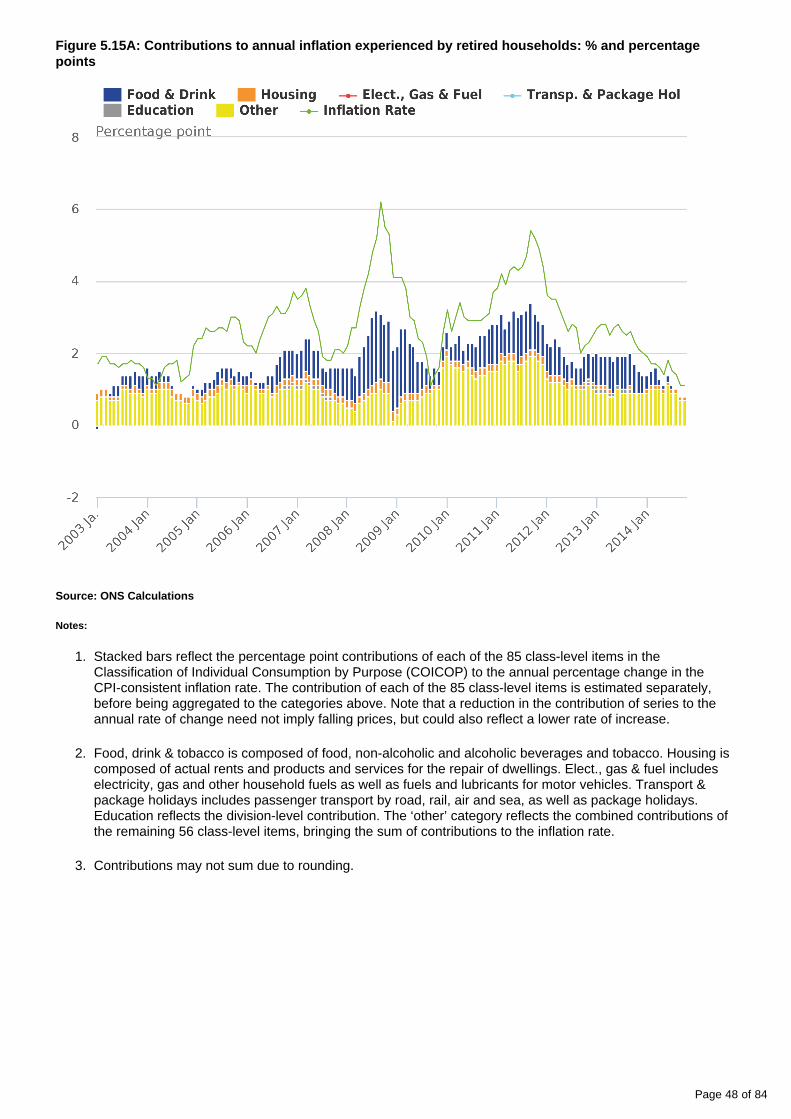
Page 48 of 84
1.
2.
3.
Figure 5.15A: Contributions to annual inflation experienced by retired households: % and percentage points
Source: ONS Calculations
Notes:
Stacked bars reflect the percentage point contributions of each of the 85 class-level items in the Classification of Individual Consumption by Purpose (COICOP) to the annual percentage change in the CPI-consistent inflation rate. The contribution of each of the 85 class-level items is estimated separately, before being aggregated to the categories above. Note that a reduction in the contribution of series to the annual rate of change need not imply falling prices, but could also reflect a lower rate of increase.
Food, drink & tobacco is composed of food, non-alcoholic and alcoholic beverages and tobacco. Housing is composed of actual rents and products and services for the repair of dwellings. Elect., gas & fuel includes electricity, gas and other household fuels as well as fuels and lubricants for motor vehicles. Transport & package holidays includes passenger transport by road, rail, air and sea, as well as package holidays. Education reflects the division-level contribution. The ‘other’ category reflects the combined contributions of the remaining 56 class-level items, bringing the sum of contributions to the inflation rate.
Contributions may not sum due to rounding.

Page 49 of 84
1.
2.
3.
Figure 5.15B: Contributions to annual inflation experienced by non-retired households: % and percentage points
Source: ONS Calculations
Notes:
Stacked bars reflect the percentage point contributions of each of the 85 class-level items in the Classification of Individual Consumption by Purpose (COICOP) to the annual percentage change in the CPI-consistent inflation rate. The contribution of each of the 85 class-level items is estimated separately, before being aggregated to the categories above. Note that a reduction in the contribution of series to the annual rate of change need not imply falling prices, but could also reflect a lower rate of increase.
Food, drink & tobacco is composed of food, non-alcoholic and alcoholic beverages and tobacco. Housing is composed of actual rents and products and services for the repair of dwellings. Elect., gas & fuel includes electricity, gas and other household fuels as well as fuels and lubricants for motor vehicles. Transport & package holidays includes passenger transport by road, rail, air and sea, as well as package holidays. Education reflects the division-level contribution. The ‘other’ category reflects the combined contributions of the remaining 56 class-level items, bringing the sum of contributions to the inflation rate.
Contributions may not sum due to rounding.

Page 50 of 84
1.
2.
3.
Figure 5.15C: Contributions to the difference in annual inflation: Retired households less non-retired households: percentage points
Source: ONS Calculations
Notes:
Stacked bars reflect the percentage point contributions of each of the 85 class-level items in the Classification of Individual Consumption by Purpose (COICOP) to the annual percentage change in the CPI-consistent inflation rate. The contribution of each of the 85 class-level items is estimated separately, before being aggregated to the categories above. Note that a reduction in the contribution of series to the annual rate of change need not imply falling prices, but could also reflect a lower rate of increase.
Food, drink & tobacco is composed of food, non-alcoholic and alcoholic beverages and tobacco. Housing is composed of actual rents and products and services for the repair of dwellings. Elect., gas & fuel includes electricity, gas and other household fuels as well as fuels and lubricants for motor vehicles. Transport & package holidays includes passenger transport by road, rail, air and sea, as well as package holidays. Education reflects the division-level contribution. The ‘other’ category reflects the combined contributions of the remaining 56 class-level items, bringing the sum of contributions to the inflation rate.
Contributions may not sum due to rounding.
Taken together, the three panels of Figure 5.15 indicate that the inflation rate of retired households has been above non-retired households’ level of inflation throughout much of the period up to late 2009. Since then, both sub-groups have alternated between experiencing the higher rates of inflation. Panels A and B suggest that many of the drivers of sub-group inflation are the same: both retired and non-retired households experienced increases in their rate of inflation during 2008 and 2011, but the former group was more affected as a consequence of its greater exposure to products with relatively high rates of inflation.
Panel C indicates that food & drink consistently push retired household price inflation above that of the non-retired. These effects are offset by smaller contributions from transport and education prices in particular. By

Page 51 of 84
Next release: To be announced
Release date: 15 December 2014
Contact: Philip [email protected]
1.
1.
comparison, the main reasons for the inflation rate differentials are the large, volatile contributions of electricity, gas & fuel. When analysed at a class-level, there are clear differences in the contributions from electricity, gas & fuel for retired and non-retired households. In general, household energy (electricity and gas) acts to increase the rate of price increases for retired households. Fuels & lubricants instead act to reduce price increases for the retired by comparison with non-retired households.
Notes for 5.4 Retired and non-retired households
Retired persons and households: A retired person is defined as anyone who describes themselves (in the LCF) as ‘retired’ or anyone over minimum National Insurance pension age describing themselves as ‘unoccupied’ or ‘sick or injured but not intending to seek work’. A retired household is defined as one where the combined income of retired members amounts to at least half the total gross income of the household.
6. Background notes
Details of the policy governing the release of new data are available by visiting www.statisticsauthority.gov. or from the Media Relations Office email: uk/assessment/code-of-practice/index.html media.relations@ons.
gsi.gov.uk
Compendium
Housing costs
Table of contents
1. Section 6. Housing costs & inflation rates
2. 6.1 CPIH and mortgage interest payments
3. 6.2 Results
4. Background notes

Page 52 of 84
1 . Section 6. Housing costs & inflation rates
While the results presented in Section 5 are consistent with the headline Consumer Prices Index (CPI) measure of inflation, they do not capture any costs of housing for those who either own their homes outright or have a mortgage. Census data suggests that owner-occupiers and owners with mortgages accounted for around 64% of the population in 2011 (ONS, 2014h), and for many of these households, the costs of housing are among their largest outlays each month. The exclusion of these costs is a shortcoming of our analysis – in particular as the prevalence of different forms of tenure will vary across different sub-groups of the population.
The appropriate treatment of housing costs in a price index is a matter of substantial debate (Leyland 2014, ILO 2004). In some cases – see, for example Crawford and Smith (2002) – it is argued that only renters and those with mortgages face changing prices for housing. It therefore follows that only expenditure on housing by this group (including both rentals and mortgage payments) should be included in an aggregate price index. For households that own their homes outright, no expenditure is recorded because changes in house prices do not affect their ‘cost of living’ in a given period. Other papers, for example Crawford (1994), argue that there is also a cost imposed on those who own their homes outright arising from the opportunity cost of investing in housing: the ‘user cost’ of housing.
2 . 6.1 CPIH and mortgage interest payments
In line with EU legislation, the UK’s headline CPI measure includes the housing costs of those renting their home, but does not include the costs of owner occupation. ONS produces two alternative indices that do capture these costs. The first of these is CPIH, which includes the housing costs of all owner-occupiers – irrespective of how they bought their home – using the ‘rental equivalence’ approach (ONS, 2014a). This is the ONS’ preferred method for measuring owner occupiers’ costs. The ‘rental equivalence’ approach involves estimating how much it would cost for owner occupiers to rent their own home under present housing market conditions, and using this ‘weight’ alongside changes in average rentals. This is closest to the ‘user cost of housing’ approach outlined above, but is challenging to adapt to our micro-level dataset. In particular, it would require detailed, household-level data on the type and form of housing tenure and geographical location, as well as a set of representative weights.
The second index – the Retail Prices Index (RPI) – includes mortgage interest payments, rentals, housing depreciation and repairs & maintenance as items in its basket of goods and services. This ensures that the RPI and RPIJ (which uses the alternative, ‘Jevons’ method to produce its elementary aggregates – rather than the ‘Carli’, which is used in the RPI) both reflect some of the housing costs experienced by both renters and owner occupiers. However, adapting this approach – and in particular producing household-level estimates of housing depreciation – is also analytically challenging.
In an effort to incorporate some of the costs that owner occupiers face, Section 3.2 and the Reference Tables outline a further set of expenditure weights which incorporates estimates of spending on each class-level item of the Classification of Individual Consumption According to Purpose (COICOP) from the Living Costs and Food Survey (LCF) with mortgage interest payments. While we recognise that this only reflects the cost of repaying a loan and fails to capture many of the costs associated with owner occupation, in particular for households who do not have mortgages, it allows us to consider a broader measure of housing costs. Repayments on the capital borrowed are not included, as these are considered to be a form of saving or investment. This section sets out the results of using this alternative set of weights. Users should note that the results of this section are not comparable with the CPI, CPIH or RPI for a range of definitional reasons: in particular as the definition of housing costs used here differs from that employed in all of these measures, and as insurance payments are included on a gross, rather than net basis.
Introducing mortgage interest payments naturally has a substantial impact on the expenditure weights for households with mortgages. On this basis, mortgage interest payments account for around 5.5% of all expenditure – only slightly lower than the 6.3% weight that actual rentals receive. As a consequence, movements in the price indices for actual rentals and mortgage interest payments can have a large impact on the aggregate price experience of households. Figure 6.1 below shows the corresponding price indices, taken from the respective CPI and RPI components. While the price of actual rentals has increased gradually over time, there was a large fall in the ‘price’ of mortgage interest payments in 2009. This corresponds to the fall in the base rate

Page 53 of 84
set by the Bank of England in response to the financial market shock and the reduction in house prices over this period.
Figure 6.1: Price indices for COICOP class 4.1.1 Actual Rentals and RPI Mortgage Interest Payments; 2002 = 100
Source: Office for National Statistics
3 . 6.2 Results
How does this impact on the inflation rate experienced by renters, those with mortgages and those who own their homes outright? Figure 6.2 shows the inflationary experience for these groups in the period 2003 to 2014 on a monthly basis. While owners with mortgages experienced higher inflation in the period 2003 to 2007 – as the price of mortgage interest payments rose at a faster rate than those for actual rentals – these households saw a sharp fall in their inflation rate to a low of -7.0% in September 2009, caused by the large fall in the price series associated with mortgage interest payments. In the most recent period, households in all three groups have experienced similar rates of inflation as the price of mortgage interest payments and actual rentals have risen at similar rates. Over the period as a whole, owners with mortgages experienced a slightly lower rate of inflation at 2.4% than either renters or owner occupiers (2.6%) .1

Page 54 of 84
1.
Figure 6.2: Annual inflation rates for renters, owners with mortgages and those who own their homes outright, including mortgage interest payments; %
Source: ONS Calculations
Notes:
Inflation rates calculated using mortgage interest payments are not comparable to CPI estimates. See Sections 3 and 6 for more details
While Figure 6.2 highlights the effect of introducing some housing costs for mortgaged owner occupiers on three sub-groups of the population, the impact on other sub-groups – including expenditure deciles, households with and without children and retired and non-retired households – will vary depending on the prevalence of different tenure forms in each group. The remainder of this section sets out the inflation experience of different household types using this alternative set of expenditure weights.
6.2.1 Inflation rates by expenditure decile, including mortgage interest payments
Figure 6.3 below shows the share of total expenditure which is accounted for by actual rentals and mortgage interest payments in each equivalised expenditure decile . First, the lowest-expenditure decile spends the least 2
on housing: together, mortgage interest payments and actual rentals account for 6.3% of total expenditure in this group, compared with 13.9% in the 4th expenditure decile. This may reflect a larger number of households living in social housing in this group – for whom housing benefit covers the costs of rent, or a high prevalence of retired households in the lower expenditure group – who are more likely to own their homes outright (see Section 6.2.2). Secondly, renting is more prevalent among the lower expenditure deciles than higher expenditure deciles: the latter spend more on mortgage interest payments on average.

Page 55 of 84
1.
Figure 6.3: Expenditure shares of mortgage interest payments and actual rentals, by equivalised expenditure deciles; %, average 2002 – 2014
Source: Living Costs and Food Survey, ONS Calculations
Notes:
Equivalised expenditure deciles (1 = lowest-expenditure households, 10 = highest-expenditure households)
These inter-decile differences in spending on housing have an impact on the inflation experience of each group. Table 6.1 shows the annual inflation rate experienced by each of the expenditure deciles in the period 2003 to 2013. The higher expenditure deciles, which contain more owners with mortgages, and who are consequently more exposed to changes in the interest rate, experience negative inflation rates in 2009 as a result of the interest rate reduction. In particular, the 9th expenditure decile experiences an inflation rate of -3.0% in 2009, which is consistent with the fact that the 9th decile has the highest share of expenditure accounted for by mortgage interest payments.
Table 6.1: Annual inflation rates for equivalised expenditure deciles, including mortgage interest payments %
%
Year Equivalised Expenditure Decile
1 2 3 4 5 6 7 8 9 10
2003 1.7 1.7 1.7 1.6 1.7 1.6 1.7 1.4 1.5 1.3
2004 2 2 2.3 2.5 2.6 2.7 2.7 2.7 2.4 2.2
2005 3.1 2.9 3 2.9 3 3 3 2.8 2.6 2.4
2006 5 4.1 3.8 3.6 3.5 3.1 3.1 2.9 2.6 2.4
2007 4.1 3.8 4.1 4.2 4.3 4.4 4.3 4.3 4.4 4.2
2008 6.7 5.9 5.3 4.8 4.6 4.2 3.8 3.6 3.3 3.1
2009 3.6 2.1 0.9 -0.4 -0.9 -1.7 -2.1 -2.7 -3 -2
2010 3.2 3.6 3.7 3.9 4 4.1 3.9 4 4 3.6
2011 5.8 5.6 5.5 5.4 5.4 5.3 5.3 5 5 4.6

Page 56 of 84
2012 3.7 3.4 3.1 3 2.8 2.8 2.7 2.6 2.6 2.6
2013 3.2 2.8 2.6 2.5 2.4 2.3 2.3 2.1 2.2 2.4
Average 3.8 3.5 3.3 3.1 3 2.9 2.8 2.6 2.5 2.4
Source: Office for National Statistics, ONS Calculations
Notes:
1. The average presented is the compound average annual growth rate, and consequently may differ from the arithmetic average of the inflation rates presented.
2. These results are not comparable with the analysis presented in Section 5, which is on a CPI-consistent basis. Differences between the inflation rates presented here include both mortgage interest payments and a range of other differences arising from differences in measurement between the LCF and the National Accounts. See Section 3 for more details.
How these differences in the annual inflation rate have affected the evolution of prices over time is shown in Figure 6.4. The effect of the fall in interest rates can be seen more clearly as the rate of price growth between 2008 and 2009 drops for expenditure deciles 4 to 10: groups that contain relatively large proportions of mortgaged home-owners. The introduction of these housing costs increases the spread of inflation rates between the 2nd and 9th expenditure deciles, opening a cumulative gap of over 10 percentage points which persists for the rest of the period. As in Section 5, the lowest-expenditure decile sees a much greater change in prices over the period compared with the highest-expenditure decile. It is important to note however that these households will only have experienced these differences if they were consistently placed in a given equivalised expenditure decile through time. As households may move between expenditure deciles through their life-cycle, the cumulative price impact presented in Figure 6.4 may not reflect their experience in aggregate precisely.
Figure 6.4: Range of cumulative price changes for equivalised expenditure deciles, selected expenditure deciles, including mortgage interest payments; 2002 = 100
Source: ONS Calculations

Page 57 of 84
1.
1.
Notes:
Figure shows the range of cumulative price change experienced by expenditure deciles between 2002 and October 2014. These results are not comparable with the analysis presented in Section 5, which is on a CPI-consistent basis. Differences between the inflation rates presented here, and in Table 6.1 above, include both mortgage interest payments and a range of other differences arising from differences in measurement between the LCF and the National Accounts. See Section 3 for more details.
6.2.2 Inflation rates for households with and without children, and retired and non-retired, including mortgage interest payments
Introducing mortgage costs in this manner also has an impact on the inflation experience of different household types. Figure 6.5 shows the share of expenditure accounted for by rentals and mortgage interest payments for households with and without children (Panel A), and for retired and non-retired households (Panel B). Panel A indicates that while rent and mortgage interest payments take equal weight for households without children, among households with children, mortgage interest payments carry more than twice the weight of rentals. Panel B highlights the greater exposure of non-retired households to housing costs – perhaps indicating that retired households are more likely to own their home outright.
Figure 6.5: Expenditure share for mortgage interest payments and actual rentals, for households with and without children (Panel A) and retired and non-retired households (Panel B); %, average 2002 – 2014
Source: Living Costs and Food Survey
Notes:
Panel A - Households without children, Households with Children. Panel B - Non-Retired Households, Retired Households
These differences in weights affect the inflation rates experienced by these different household types. Figure 6.6 below shows the annual inflation rates for households with and without children, after incorporating mortgage interest payments. As households with children are more exposed to changes in the interest rate through greater expenditure on mortgage interest payments, they benefitted from the fall in interest rates in 2009 to a greater extent. Between 2008 and 2012, their inflation rate was generally below that of households without children,
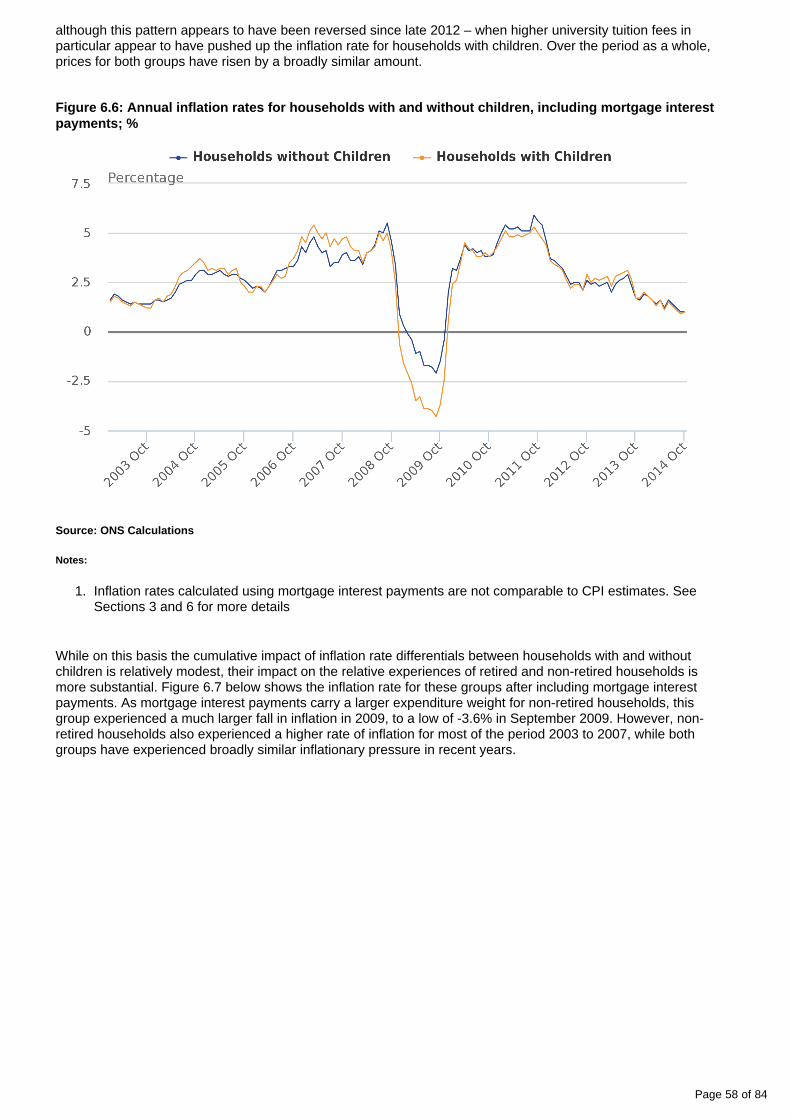
Page 58 of 84
1.
although this pattern appears to have been reversed since late 2012 – when higher university tuition fees in particular appear to have pushed up the inflation rate for households with children. Over the period as a whole, prices for both groups have risen by a broadly similar amount.
Figure 6.6: Annual inflation rates for households with and without children, including mortgage interest payments; %
Source: ONS Calculations
Notes:
Inflation rates calculated using mortgage interest payments are not comparable to CPI estimates. See Sections 3 and 6 for more details
While on this basis the cumulative impact of inflation rate differentials between households with and without children is relatively modest, their impact on the relative experiences of retired and non-retired households is more substantial. Figure 6.7 below shows the inflation rate for these groups after including mortgage interest payments. As mortgage interest payments carry a larger expenditure weight for non-retired households, this group experienced a much larger fall in inflation in 2009, to a low of -3.6% in September 2009. However, non-retired households also experienced a higher rate of inflation for most of the period 2003 to 2007, while both groups have experienced broadly similar inflationary pressure in recent years.

Page 59 of 84
1.
Figure 6.7: Annual inflation rates for retired and non-retired households, including mortgage interest payments, %
Source: ONS Calculations
Notes:
Inflation rates calculated using mortgage interest payments are not comparable to CPI estimates. See Sections 3 and 6 for more details
The cumulative impact of these annual rates of inflation is shown in Figure 6.8. As retired households did not benefit as much from the fall in interest rates, the price experience of these sub-groups diverged in 2009, and the gap has persisted over the following five years. Prices have risen for retired households by 40.7% in the period 2002 to October 2014, while prices for non-retired households have risen by 35.9% over the same period.

Page 60 of 84
1.
1.
2.
1.
Figure 6.8: Cumulative price changes for retired and non-retired households, including mortgage interest payments, 2002 = 100
Source: ONS Calculations
Notes:
Figure shows the range of cumulative price changes of products purchased by the respective groups between 2002 and October 2014. These results are not comparable with the analysis presented in Section 5, which is on a CPI-consistent basis. Differences between the inflation rates presented here, and in Table 6.1 above, include both mortgage interest payments and a range of other differences arising from differences in measurement between the LCF and the National Accounts. See Section 3 for more details.
Notes for 6.2 Results
The average presented is the compound average annual growth rate, and consequently may differ from the arithmetic average of the inflation rates presented.
For each dataset listed in Section 3.2, equivalised expenditure deciles are created based on the respective measure of expenditure. In this section, expenditure based on the LCF and mortgage interest payments is used to create the expenditure deciles.
4. Background notes
Details of the policy governing the release of new data are available by visiting www.statisticsauthority.gov. or from the Media Relations Office email: uk/assessment/code-of-practice/index.html media.relations@ons.
gsi.gov.uk
Compendium

Page 61 of 84
Next release: To be announced
Release date: 15 December 2014
Contact: Philip [email protected]
Democratic indices
Table of contents
1. Section 7. Democratic indices
2. 7.1 Results
3. Background notes

Page 62 of 84
1.
1 . Section 7. Democratic indices
In common with many modern price indices, the Consumer Prices Index (CPI) weights the price movements of items in proportion to their importance to total household spending. Price movements for products on which households spend a large fraction of their income are consequently weighted more heavily than items on which households spend relatively little.
As discussed in Section 2, a corollary of this approach is that high-spending households have a greater weight in the CPI than low-spending households. This follows because high-spending households influence total households’ spending to a greater extent than low-spending households. However, an alternative to this approach is to calculate a price index in which each household receives an equal weight. These price indices – commonly referred to as ‘democratic ’ price indices – capture a degree of the variation in expenditure weights 1
across households in a population. In populations with homogenous weights – where all households purchase goods in equal proportions – the ‘plutocratically’ weighted CPI and the democratic index are equal. The more variation there is in expenditure baskets across households – perhaps because of differing tastes, interests or income constraints – the larger the difference between these indices. While the conventional democratic price index is for all households in an economy, the logic applies equally to any chosen sub-group.
To shed some light on this matter in the UK context, this section compares the headline, plutocratically-weighted, CPI with the democratically-weighted index for the UK between 2002 and 2014. It proceeds to present democratic price indices for households with and without children, and retired and non-retired households.
Notes for section 7. Democratic indices:
Note that the naming convention here can be misleading: In a ‘democratic’ index, each household is given an equal weight, rather than each individual, which might be implied from its name. A ‘truly’ democratic index would weight each person in an economy equally, and would deviate from the popular convention of a democratic index to the extent of variation in household size. Arguably, a still ‘truer’ index would use longitudinal data to observe movements in expenditure patterns for the same individuals through time, however, this approach is data-intensive, challenging to implement, and its interpretation not straightforward.
2 . 7.1 Results
7.2.1 All households
Weighting households equally – rather than according to their expenditure (see Section 2) – means that a democratic price index will more closely reflect the price experience of low expenditure households than a conventional plutocratically-weighted index. As the results presented in Section 5 suggest that low-expenditure households have typically experienced higher rates of inflation than high-expenditure households over the last decade, it should come as little surprise that the democratic index shows a higher rate of inflation than the CPI. This is shown in Figure 7.1, which plots both series between January 2003 and October 2014. Only in 2010 and 2014 to date – when the range of inflation outcomes between deciles narrows markedly (see Figure 5.5) – is the gap between the two negligible.

Page 63 of 84
Figure 7.1: CPI-consistent democratic and plutocratic inflation rates for all households, %
Source: ONS Calculations
While Figure 7.1 above shows the democratically- and plutocratically-weighted price indices for the period January 2003 and October 2014, Figure 7.2 shows the difference between the two series. It indicates that the CPI is on average around 0.3 percentage points lower than an equivalent index in which every household is given an equal weight over this period. In 2008, this difference was particularly marked, while in late 2009 to early 2010 and in recent months in 2014, the difference was close to zero. While assessing the statistical significance of these differences is difficult, the underlying trend is clear: during periods when the degree of variation in household inflation experiences is much broader (see Figure 5.5), the extent of the difference between these indices is greater. In line with the analysis presented in Section 5, this effect is particularly noticeable in 2006, 2008 and 2011: periods in which the average rate of inflation rises quite sharply.
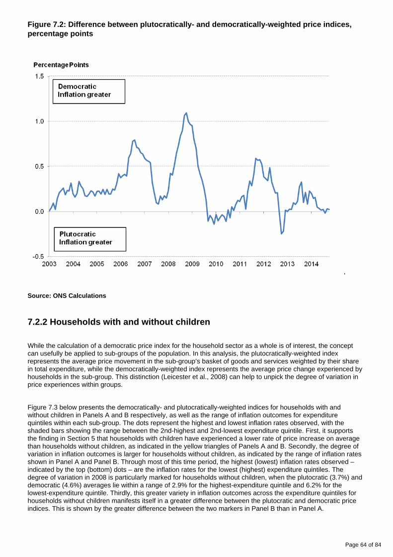
Page 64 of 84
Figure 7.2: Difference between plutocratically- and democratically-weighted price indices, percentage points
Source: ONS Calculations
7.2.2 Households with and without children
While the calculation of a democratic price index for the household sector as a whole is of interest, the concept can usefully be applied to sub-groups of the population. In this analysis, the plutocratically-weighted index represents the average price movement in the sub-group’s basket of goods and services weighted by their share in total expenditure, while the democratically-weighted index represents the average price change experienced by households in the sub-group. This distinction (Leicester et al., 2008) can help to unpick the degree of variation in price experiences within groups.
Figure 7.3 below presents the democratically- and plutocratically-weighted indices for households with and without children in Panels A and B respectively, as well as the range of inflation outcomes for expenditure quintiles within each sub-group. The dots represent the highest and lowest inflation rates observed, with the shaded bars showing the range between the 2nd-highest and 2nd-lowest expenditure quintile. First, it supports the finding in Section 5 that households with children have experienced a lower rate of price increase on average than households without children, as indicated in the yellow triangles of Panels A and B. Secondly, the degree of variation in inflation outcomes is larger for households without children, as indicated by the range of inflation rates shown in Panel A and Panel B. Through most of this time period, the highest (lowest) inflation rates observed – indicated by the top (bottom) dots – are the inflation rates for the lowest (highest) expenditure quintiles. The degree of variation in 2008 is particularly marked for households without children, when the plutocratic (3.7%) and democratic (4.6%) averages lie within a range of 2.9% for the highest-expenditure quintile and 6.2% for the lowest-expenditure quintile. Thirdly, this greater variety in inflation outcomes across the expenditure quintiles for households without children manifests itself in a greater difference between the plutocratic and democratic price indices. This is shown by the greater difference between the two markers in Panel B than in Panel A.
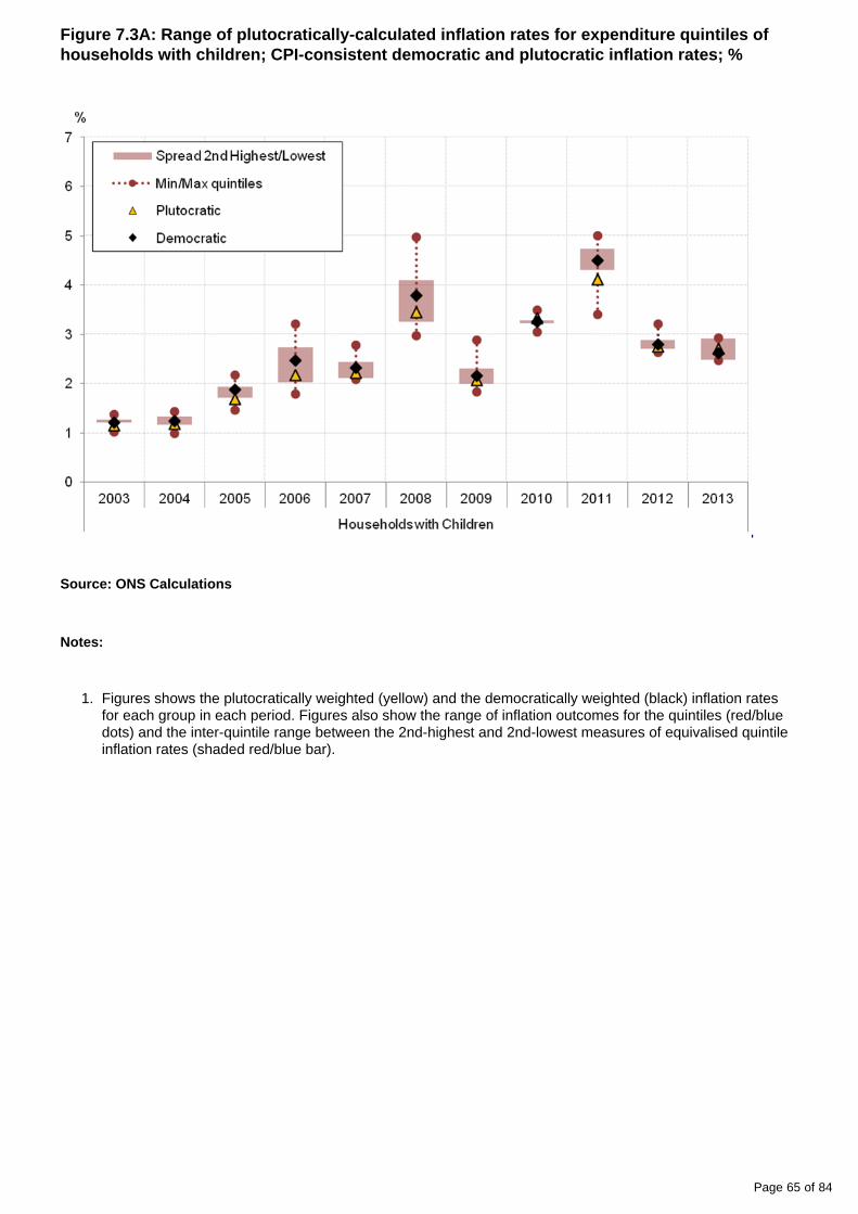
Page 65 of 84
1.
Figure 7.3A: Range of plutocratically-calculated inflation rates for expenditure quintiles of households with children; CPI-consistent democratic and plutocratic inflation rates; %
Source: ONS Calculations
Notes:
Figures shows the plutocratically weighted (yellow) and the democratically weighted (black) inflation rates for each group in each period. Figures also show the range of inflation outcomes for the quintiles (red/blue dots) and the inter-quintile range between the 2nd-highest and 2nd-lowest measures of equivalised quintile inflation rates (shaded red/blue bar).

Page 66 of 84
1.
Figure 7.3B: Range of plutocratically-calculated inflation rates for expenditure quintiles of households without children; CPI-consistent democratic and plutocratic inflation rates; %
Source: ONS Calculations
Notes:
Figures shows the plutocratically weighted (yellow) and the democratically weighted (black) inflation rates for each group in each period. Figures also show the range of inflation outcomes for the quintiles (red/blue dots) and the inter-quintile range between the 2nd-highest and 2nd-lowest measures of equivalised quintile inflation rates (shaded red/blue bar).
What explains these differences? As in Section 5 above, the inflation rate differentials shown here are driven by differences in expenditure patterns. Households without children consequently appear to be a more heterogeneous group than households with children, spending more on average on products whose price has increased relatively sharply over this period. Much of this difference is likely due to the demographic composition of these groups, as retired and elderly households are concentrated in the households without children group.
7.2.3 Retired households
Section 5 indicated that retired households have experienced higher rates of inflation than non-retired households on average since 2003, largely as a consequence of retired households spending more of their income on products that have risen strongly in price over this period.
Figure 7.4 presents the plutocratically- (yellow) and democratically-weighted (black) inflation rates for retired (Panel A) and non-retired households (Panel B). The two panels also summarise the distribution of inflation rates for these groups, showing the range of inflation outcomes for expenditure quintiles in each group. The dots represent the highest and lowest quintile-level inflation rates observed, with the shaded bars showing the range between the 2nd-highest and 2nd-lowest quintile results. As reported above, the average rate of price increase

Page 67 of 84
1.
for retired households is higher than for non-retired households, but it is the difference in the range of inflation outcomes that is particularly striking. On average, the range of inflation outcomes across the expenditure quintiles of the retired population is around twice as broad as the equivalent range for non-retired households. In 2008, while inflation outcomes for the non-retired population ranged from 2.9% to 5.0%, the equivalent range for the retired population was 3.0% to 7.1%. While some retired households experienced broadly the same inflation rate as the non-retired population, a subset of this group faced much faster rates of price increase.
Figure 7.4A: Range of plutocratically-calculated inflation rates for expenditure quintiles of retired households; CPI-consistent democratic and plutocratic inflation rates; %
Source: ONS Calculations
Notes:
Figures shows the plutocratically weighted (yellow) and the democratically weighted (black) inflation rates for each group in each period. Figures also show the range of inflation outcomes for the quintiles (red/blue dots) and the inter-quintile range between the 2nd-highest and 2nd-lowest measures of equivalised quintile inflation rates (shaded red/blue bar).
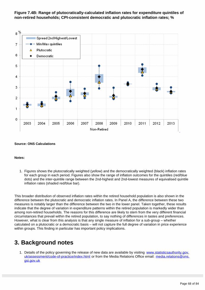
Page 68 of 84
1.
1.
Figure 7.4B: Range of plutocratically-calculated inflation rates for expenditure quintiles of non-retired households; CPI-consistent democratic and plutocratic inflation rates; %
Source: ONS Calculations
Notes:
Figures shows the plutocratically weighted (yellow) and the democratically weighted (black) inflation rates for each group in each period. Figures also show the range of inflation outcomes for the quintiles (red/blue dots) and the inter-quintile range between the 2nd-highest and 2nd-lowest measures of equivalised quintile inflation rates (shaded red/blue bar).
This broader distribution of observed inflation rates within the retired household population is also shown in the difference between the plutocratic and democratic inflation rates. In Panel A, the difference between these two measures is notably larger than the difference between the two in the lower panel. Taken together, these results indicate that the degree of variation in expenditure patterns within the retired population is markedly wider than among non-retired households. The reasons for this difference are likely to stem from the very different financial circumstances that prevail within the retired population, to say nothing of differences in tastes and preferences. However, what is clear from this analysis is that any single measure of inflation for a sub-group – whether calculated on a plutocratic or a democratic basis – will not capture the full degree of variation in price experience within groups. This finding in particular has important policy implications.
3. Background notes
Details of the policy governing the release of new data are available by visiting www.statisticsauthority.gov. or from the Media Relations Office email: uk/assessment/code-of-practice/index.html media.relations@ons.
gsi.gov.uk

Page 69 of 84
Next release: To be announced
Release date: 15 December 2014
Contact: Philip [email protected]
Compendium
Limitations
Table of contents
1. Section 8. Limitations
2. 8.1 Common price indices
3. 8.2 Aligning micro-level expenditure data and CPI weights
4. 8.3 Data sources
5. Background notes

Page 70 of 84
1 . Section 8. Limitations
While the calculation of inflation rates for subsets of the household population is analytically straightforward, a range of data constraints make their estimation challenging in practice. As a result, this paper and others in the field make a range of simplifying assumptions. This section discusses these assumptions and the limits of our analysis with the aim of identifying areas for future work.
2 . 8.1 Common price indices
Perhaps the most important limitation of this analysis is the use of national price indices alongside sub-group specific expenditure weights. As set out in Section 2, an analysis of sub-group specific inflation rates would ideally use price indices and expenditure weights specific to each household . While the expenditure weights 1
used here capture differences in the consumption patterns of different households, the lack of sub-group specific price indices means that this and other papers assume that all households face the same prices.
While this may be a fair assumption for some items – TV licences for instance, for which there is little variation in price – it is less likely to hold in product categories which comprise large numbers of heterogeneous items – such as second-hand cars or photographic, cinematographic & optical equipment. In these categories, the products included in the Consumer Prices Index (CPI) are selected to be representative of the purchases of all households and therefore capture ‘average’ price movements. As a result, they may be more or less representative of the prices that sub-groups experience.
The impact of this assumption on our analysis depends on the extent to which households face different prices for goods in the same COICOP class and on the extent to which within-class prices move together. As is summarised in Table 8.1 below, when different types of households purchase broadly similar types of goods within each COICOP class and when intra-class price movements are similar, the impact of our assumption 2
should be relatively small (top left quadrant). The greatest impact of the assumption arises where households are highly differentiated in their within-class purchases, and when the prices of those products move in very different directions (bottom right).
Table 8.1: Impact of intra-class price and product differentiation on sub-group inflation estimates
Degree of intra-class price integration Degree of between household variation in within-class product purchases
Households buy similar within-class products
Households buy different within-class products
Intra-class product prices move at a similar rate
Low Moderate-High
Intra-class product prices move at different rates
Low-Moderate High
Source: Office for National Statistics
As data on the degree to which prices vary for different types of household are not available, it is not possible to quantify the impact of this limitation with any precision. Academic work on this topic is also limited: two studies based on households in the United States – Broda, Leibtag and Weinstein (2009), and Aguiar and Hurst (2007) – suggest that there is evidence of differential pricing for different household types, but as yet there is no comparable evidence for the UK. However, Figures 8.1 and 8.2 give some broad sense of its potential importance. Figure 8.1 shows the proportion of household food expenditure that is accounted for by sub-components of bread & cereals by equivalised income quintile in 2012. It shows that households vary in the type of within-class products that they purchase, with households in lower income quintiles allocating a greater share of their expenditure to bread in particular, than higher-income households. As these within-class and between-household differences in expenditure patterns are likely to vary in magnitude with the nature of the product considered, Figure 8.1 suggests that future work could usefully document these differences and take account of them in the calculation of household-level inflation rates.

Page 71 of 84
Figure 8.1: Food expenditure share allocated to sub-components of bread & cereals COICOP class by equivalised income quintile, %, 2012
Source: Living Costs and Food Survey - Office for National Statistics
If there is some evidence of within-class differences in expenditure patterns, to what extent do the prices for these different products vary through time? Figure 8.2 explores this question using the micro-level price quote data on which the CPI is constructed. It shows the distribution of price growth observed for four different types of bread in 2012. The price of branded white loaves of bread for instance, has increased by around 7.5% over this period, while the price of six bread rolls increased by just 2.3%. If these differences are replicated in different classes and over different time periods, then the impact of our assumption may be relatively large.
Figure 8.2: Prices of selected ‘bread’ products: January 2012=100
Source: Office for National Statistics

Page 72 of 84
1.
2.
Taken together, Figures 8.1 and 8.2 suggest that there is potential for the results presented in this paper to be affected by within-class differences in expenditure and price growth. However, without more detailed information on both expenditure and prices, it is not possible to estimate either the direction or the size of this effect. This challenge we leave to future work.
Notes for 8.1 Common price indices
See Section 3 for more details.
COICOP is the Classification of Individual Consumption According to Purpose. See Section 2 and Appendix B for more detail.
3 . 8.2 Aligning micro-level expenditure data and CPI weights
A second set of assumptions used in this paper concerns the methods that are used to harmonise the micro-level expenditure data from the Living Costs and Food Survey (LCF) and the expenditure weights that are used in the construction of the Consumer Prices Index. As set out in Section 3.1 above, these may differ for a range of reasons, but in particular because the LCF is not the sole source of expenditure data in the CPI. The broad method used to harmonise these two sets of expenditure data is set out in Section 3.2, and involves the allocation of the CPI expenditure totals to observed LCF households in proportion to the spending that they report in the LCF.
Harmonising the CPI expenditure weights with the micro-level data from the LCF in this way requires several assumptions. First, we assume that the distribution of household-level spending on each COICOP class reported in the LCF is representative of the ‘true’ underlying distribution. This, apparently anodyne assumption has two important corollaries: (a) that households do not censor their spending patterns in the LCF; and (b) that all types of households are equally likely to over- or under-state expenditure on a given product type. To see the importance of these assumptions, consider spending on alcohol and tobacco, both of which are thought to be under-recorded by the LCF (ONS, 2014d). The first corollary states that no household reports zero expenditure on these categories if they have strictly positive expenditure on alcohol and tobacco during the reporting period. The second corollary implies that – having met this first condition – no household type is more or less likely to over- or under-report spending on alcohol or tobacco. Both assumptions are relatively strong, and unfortunately there is no way to estimate the impact of these biases without additional data .1
Secondly, where the expenditure weight in the CPI is based on data other than the household survey, the differences between the LCF and CPI expenditure totals can be large (see Figure 3.3). To assess the effect of allocating these new expenditure totals to the observed household units, we conducted a set of plausibility checks. The first of these is presented in Figure 8.3 below. The horizontal axis shows the difference between the LCF and the CPI expenditure total as a proportion of the LCF total: numbers close to 100 therefore indicate close correspondence between the two weights, while observations further from 100 indicate greater differences. The vertical axis plots the number of households who report strictly positive expenditure. Each point is a single COICOP class, representing expenditure on a given set of products. The chart is divided into four shaded ‘zones’. In the top left are COICOP classes in which the LCF and CPI expenditure totals are of broadly similar orders of magnitude (defined as CPI expenditure less than double the LCF total) and where the number of households reporting strictly positive expenditure is relatively high (defined as above 20%). In this segment are many products for which the LCF is taken as the basis for the CPI weights. Immediately below this quadrant are instances where the number of households reporting strictly positive expenditure is relatively small, but where the CPI and LCF expenditure totals are fairly similar. Points in these two quadrants will introduce the least potential bias.

Page 73 of 84
1.
2.
Figure 8.3: Difference between LCF and CPI as a % of LCF and % Households reporting positive expenditure, average 2002-2014
Source: ONS Calculations
Notes:
Figure is a scatter plot showing the 85 class-level categories of the CPI. The vertical axis plots the percentage of surveyed households who report some expenditure on that class-level item. The horizontal axis shows the percentage difference between the expenditure total in the CPI and LCF.
The Figure excludes class-level category 06.3.1: Medical & paramedic services as the CPI expenditure total is around 230 times bigger than in the LCF.
Points in the top right hand quadrant, by contrast, represent classes where CPI expenditure is high relative to the LCF total, and where a relatively large number of households have reported positive spending. In these cases, the potential for bias is also limited, as a large proportion of households will be affected by the micro-level attribution mechanism. However, it is points in the bottom right-hand quadrant that present the most difficulty: these are COICOP classes in which the CPI expenditure total is more than double the LCF total, and in which fewer than 20% of households report spending. Medical & paramedic services remains an outlier, with just 66 households reporting spending on this COICOP class-level over the eleven years of available data.
In these cases, and where the proportion of LCF respondents reporting expenditure is relatively small, we adjust our methodology to avoid perverse results. Implementing this adjustment requires the assumption that it is appropriate to allocate total spending on a COICOP class (6.3.1 Medical & paramedic services, for instance) using reported household expenditure on a higher aggregate – (6 Health, for instance). This assumption ensures that our methodology does not allocate very high levels of spending to a relatively small number of households, which in turn would distort the picture of household inflation.
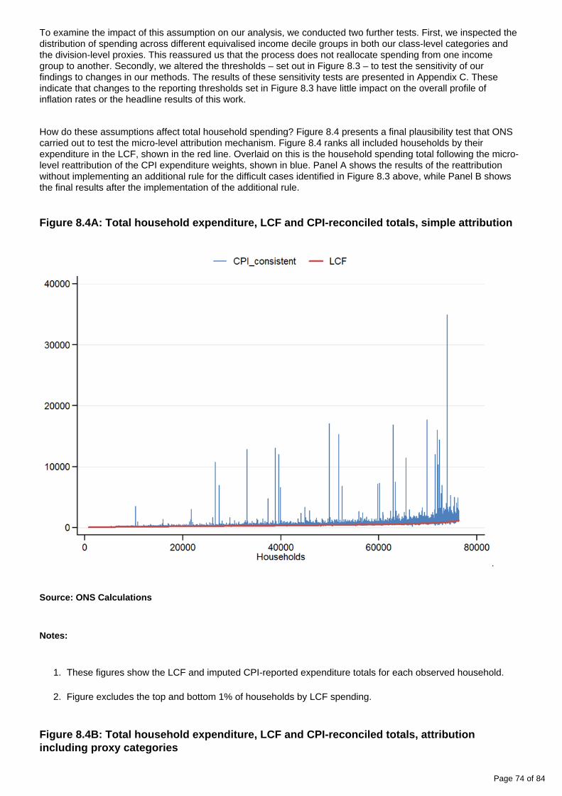
Page 74 of 84
1.
2.
To examine the impact of this assumption on our analysis, we conducted two further tests. First, we inspected the distribution of spending across different equivalised income decile groups in both our class-level categories and the division-level proxies. This reassured us that the process does not reallocate spending from one income group to another. Secondly, we altered the thresholds – set out in Figure 8.3 – to test the sensitivity of our findings to changes in our methods. The results of these sensitivity tests are presented in Appendix C. These indicate that changes to the reporting thresholds set in Figure 8.3 have little impact on the overall profile of inflation rates or the headline results of this work.
How do these assumptions affect total household spending? Figure 8.4 presents a final plausibility test that ONS carried out to test the micro-level attribution mechanism. Figure 8.4 ranks all included households by their expenditure in the LCF, shown in the red line. Overlaid on this is the household spending total following the micro-level reattribution of the CPI expenditure weights, shown in blue. Panel A shows the results of the reattribution without implementing an additional rule for the difficult cases identified in Figure 8.3 above, while Panel B shows the final results after the implementation of the additional rule.
Figure 8.4A: Total household expenditure, LCF and CPI-reconciled totals, simple attribution
Source: ONS Calculations
Notes:
These figures show the LCF and imputed CPI-reported expenditure totals for each observed household.
Figure excludes the top and bottom 1% of households by LCF spending.
Figure 8.4B: Total household expenditure, LCF and CPI-reconciled totals, attribution including proxy categories

Page 75 of 84
1.
2.
1.
Source: ONS Calculations
Notes:
These figures show the LCF and imputed CPI-reported expenditure totals for each observed household.
Figure excludes the top and bottom 1% of households by LCF spending
Panel A suggests that without the additional rule, the simplest reattribution of the CPI weights adjusts total expenditure for some households considerably, as is shown by the ‘spiky’ blue line. In these cases, adjusted spending is substantially higher than the LCF total, which in turn points to a risk that our method is affecting the results. However, after the implementation of the additional rule in Panel B, the distribution of expenditure is broadly maintained, and very few households’ expenditure totals are substantially distorted. These results, and the broad similarity between the results of the LCF and CPI-consistent analysis, give us confidence that our results are the product of well-defined trends in household experience, rather than our methods.
Finally, it is worth noting that this alignment process delivers a micro-level expenditure dataset that is consistent with the CPI weights, not with the National Accounts. The difference here arises because – as discussed in Section 3 above – the CPI weights are price up-dated from a previous year and are not revised. Implicit in this mechanism is the assumption that households do not substitute in the face of changing prices between the point of survey and the fixing of the expenditure weights. For our work, this implies that while the alignment process delivers the CPI weights exactly, it will not deliver the National Accounts expenditure totals.
Notes for 8.2 aligning micro-level expenditure data and CPI weights
In principle, it is possible to estimate ‘imputed’ values for households who do not report any expenditure in a given COICOP. This would be likely to involve a two-step model, first estimating the likelihood of positive

Page 76 of 84
Next release: To be announced
Release date: 15 December 2014
Contact: Philip [email protected]
1.
1.
expenditure on a given product, before estimating the extent of that expenditure. However, this approach involves a further set of explicit and implicit assumptions. Here, we have chosen to keep our approach simple and leave this line of inquiry for future research.
4 . 8.3 Data sources
There is also a range of additional limitations that relate to the data sources used in this paper, rather than the methods employed to calculate price indices and inflation rates. First, while the LCF is a relatively large, continuous survey of household expenditure, it places a burden on respondents. As a result, the response rate varies – ranging between 50% and 60%. As there are no obvious candidate variables that could be used as exclusion restrictions, we have not been able to model this process of non-response. This may affect our results if non-reporting households have very different patterns of expenditure to those who do report, although non-response weighting is used throughout to alleviate this issue. Analysis of the response rate suggests that some types of household are less likely to respond to the LCF (Bright et al., 2009), but without more detailed information it is difficult to assess the likely size or direction of this effect. Secondly, the LCF does not cover some types of household that might be of interest. In particular, it does not cover student halls and other communal establishments.
Thirdly, housing costs are a further area of weakness in our work. In particular, the lack of information required to produce micro-level estimates of rental equivalence, the ONS’ preferred measure, means that the price indices calculated here – while consistent with the national CPI – exclude the costs associated with housing for a large number of households. This limitation is particularly concerning, because it is likely to have a differential impact across some of the sub-groups of interest. For instance, renters (whose housing costs are captured in this work) are more prevalent among low-income, low-expenditure and non-retired households than owner-occupiers (whose housing costs are less well captured), who are more likely to be in the high-income, high-expenditure and retired household groups. All of these issues we leave for future work.
5. Background notes
Details of the policy governing the release of new data are available by visiting www.statisticsauthority.gov. or from the Media Relations Office email: uk/assessment/code-of-practice/index.html media.relations@ons.
gsi.gov.uk
Compendium
Conclusions
Table of contents
1. Introduction
2. Conclusions
3. Background notes

Page 77 of 84
1 . Introduction
Conclusions from the ONS analysis of the inflation rates experienced by different types of households in the UK between 2003 and 2014 are presented in this section.
2 . Conclusions
This paper presents ONS analysis of the inflation rates experienced by different types of households in the UK between 2003 and 2014. Using micro-level data from the Living Costs and Food Survey (LCF) and the Consumer Prices Index (CPI), it estimates price indices and inflation rates for households in each decile of the income and expenditure distributions, for households with and without children, and for retired and non-retired households.
This analysis draws a number of conclusions. First, the rate of inflation experienced by different types of household has varied markedly since 2003. These differences are most apparent when comparing households who spend relatively little with those who spend the most. Prices rose each year for the lowest-expenditure decile on average by 3.7%, compared with 2.3% for the highest-expenditure decile. Comparing the 2nd and 9th expenditure deciles – our preferred measure – this difference remains substantial: prices for the former group 1
have risen on average by 3.3% each year over this period, while for the latter they have risen by 2.3%. The CPI over this period – which is designed to capture price movement for the household sector as a whole – has risen by 2.6% each year on average.
While the extent of inflation differentials is largest among households with different levels of expenditure, this analysis also indicates that there are inflation rate differentials for other sub-groups in the population. Prices have risen faster on average for households in lower income groups, for retired households and for households without children than for high income, non-retired and households with children respectively. Supporting analysis suggests that housing costs have also played an important role: groups with a greater incidence of mortgaged owner-occupiers have experienced lower rates of price increase over this period as a consequence of lower mortgage interest payments.
While the movements in some prices have influenced all groups, their importance as drivers of inflation has differed substantially. Retired households were particularly exposed to the movements of energy and food prices over this period, but were much less affected by the increasing price of education (led by higher university tuition fees) and package holidays. Households with children, by contrast, were more exposed to price changes for education, and less exposed to movements in energy and transport costs. Comparing high and low expenditure groups, changes in the costs of utilities, food and drink account for most of the differences in inflation rates.
This paper also documents the degree of variation in rates of price increase within sub-groups. In particular, it concludes that the range of inflation outcomes for retired households is far broader than the range of inflation outcomes for non-retired households. Among the former group, a majority experienced broadly similar rates of price increase to the rest of the population. A minority of retired households experienced much faster rates of price increase, rising to more than 7% in 2008. This result for retired households suggests that the expenditure patterns of this group are diverse relative to non-retired households. Comparing the CPI with the inflation outturns for different groups, this paper concludes that the CPI is broadly representative of the price experience of households around two-thirds of the way up the expenditure distribution. An alternative, ‘democratic’ price index – which weights the inflation experience of households equally, rather than drawing on household sector expenditure weights – is around 0.3 percentage points higher on average than the plutocratic measure over this period.
Our findings have several implications, of which two are particularly clear. First, it is apparent that while the CPI captures movements in prices for the household sector as a whole, the degree of variation in the price experience of different households is relatively broad. Rates of price increase vary systematically across household types and composition, to differing degrees in different periods. That degree of variation needs consideration alongside movements in the headline rate of CPI inflation. A first step towards greater understanding and appreciation of these differences would be for a distributional analysis of inflation trends to be published on a regular basis. In

Page 78 of 84
Next release: To be announced
Release date: 15 December 2014
Contact: Philip [email protected]
1.
1.
line with our findings, this should incorporate estimates of within-group inflation differentials, as well as between group differences. This would allow these differentials to be monitored through time, to see whether the trends observed during this period are sustained as the economy continues to recover.
Secondly, the degree of variation presented here has broader implications for economic policy. In particular, it suggests that some sub-groups of the UK population have faced relatively strong headwinds in recent years, eroding both their real incomes and their capacity to spend. The results also suggest that when inflation is relatively high, the dispersion of inflation outcomes is relatively broad. Both effects suggest that distributional analysis of current macroeconomic developments can offer significant insights into conditions prevailing in the UK economy.
This paper presents a range of avenues for further study, developing on the methods we have employed here. First, future research could seek to quantify the extent to which different households face different prices for the same product. In common with previous studies, this paper assumes that all households face the same, CPI price indices and as a consequence, inflation differentials are driven by expenditure shares alone. If different households face different prices for the same products, and if these prices grow at different rates, then their experience of inflation may differ from the estimates presented here. Secondly, further work could be carried out to extend our findings from CPI to CPIH – allowing housing costs for all households to be included in the sub-group inflation estimates.
Notes for Conclusions
This measure is less affected by unusually low- or high-expenditure households who appear in our underlying data. Lower (higher) decile numbers denote lower (higher) expenditure groups.
3. Background notes
Details of the policy governing the release of new data are available by visiting www.statisticsauthority.gov. or from the Media Relations Office email: uk/assessment/code-of-practice/index.html media.relations@ons.
gsi.gov.uk
Compendium
List of Appendices
Table of contents
1. Appendix A
2. Appendix B
3. Appendix C
4. Background notes

Page 79 of 84
1 . Appendix A
Difference between Lowe and Laspeyres
Within the year the Consumer Prices Index (CPI) is calculated using a Lowe formula, in the sense that it uses current-period price information alongside expenditure weights that are price-updated. This latter feature distinguishes it from a Laspeyres price index, which uses current period price information with observed, previous period expenditure weights. The Laspeyres is presented algebraically below in [A.1]:
Equation A.1
This formula can also be written in terms of expenditure shares and prices relatives, which indicates how the formula is applied in practice. This is outlined in [A.2]:
Equation A.2
The formula for a Lowe price index differs in the sense that the expenditure shares from an earlier period are price updated to deliver a set of weights for a period before the expenditure data for that period becomes available. This earlier period is denoted as b, shown in [A.3]:
Equation A.3
2 . Appendix B
Structure of the Classification of Individual Consumption According to Purpose (COICOP)
The table for Appendix B are available as a within this release.reference table download (30 Kb Excel sheet)
3 . Appendix C

Page 80 of 84
Sensitivity analysis
This appendix provides further information about how this paper adjusts the methodology for those class-level categories where the CPI expenditure total is more than double the LCF total, and in which fewer than 20% of households report spending. The sensitivity analysis undertaken to ensure this adjustment has not biased the headline results is also outlined.
Table C.1 shows the class-level categories where the adjustment has been applied. The right-hand side outlines which other class-level categories are used as a ‘proxy’ to allocate the CPI expenditure according to the total of all these categories as a share of total expenditure. Proxies are chosen as follows: a) if the class-level category is contained within a group with other class-levels, the proxy is the sum of all classes of the group; and b) if the class-level category is the only class within a group, the proxy is the sum of all classes of the division. These proxies have been checked to ensure the distributions of expenditure by equivalised income decile and year are not biased by this allocation.
Table C.1: Class-level categories and their respective proxies
Class-level Category
Proxy
03.1.3 03.1.2 + 03.1.3 + 03.1.4
04.3.1 04.3.1 + 04.3.2
04.4.3 04.4.3 + 04.4.1
04.5.4 04.5.1 + 04.5.2 + 04.5.3 + 04.5.4
05.2.1 05.1.1 + 05.1.2 + 05.2.1 + 05.3.1 + 05.3.3 + 05.4.1 + 05.5.1 + 05.6.1 + 05.6.2
06.3.1 06.1.1 + 06.1.2.3 + 06.2.1.3 + 06.2.2 + 06.3.1
07.1.2 07.1.1a + 07.1.1b + 07.1.2
07.3.4 07.3.1 + 07.3.2 + 07.3.3 + 07.3.4
09.1.2 09.1.1 + 09.1.2 + 09.1.3 + 09.1.4 + 09.1.5
09.1.5 09.1.1 + 09.1.2 + 09.1.3 + 09.1.4 + 09.1.5
09.2.1 09.1.1 + 09.1.2 + 09.1.3 + 09.1.4 + 09.1.5 + 09.2.1 + 09.3.1 + 09.3.2 + 09.3.3 + 09.3.4 + 09.4.1 + 09.4.2 + 09.5.1 + 09.5.2 + 09.5.3 + 09.6.1
12.3.1 12.3.1 + 12.3.2
12.4.1 12.1.1 + 12.1.2 + 12.3.1 + 12.3.2 + 12.4.1 + 12.5.2 + 12.5.3 + 12.5.4 + 12.6.2 + 12.7.1
12.7.1 12.1.1 + 12.1.2 + 12.3.1 + 12.3.2 + 12.4.1 + 12.5.2 + 12.5.3 + 12.5.4 + 12.6.2 + 12.7.1
Source: ONS Calculations
As part of the plausibility tests, the condition was extended to include all class-level categories where CPI expenditure total is more than double the LCF total. This added eight class-level categories to the analysis. Table C.2 outlines these class-level categories and their respective proxies.
Table C.2: Sensitivity analysis of class-level categories, and their respective proxies
Class-level Category
Proxy
02.2.1 02.1.1 + 02.1.2 + 02.1.3 + 02.2.1
04.3.2 04.3.1 + 04.3.2
05.4.1 05.1.1 + 05.1.2 + 05.2.1 + 05.3.1 + 05.3.3 + 05.4.1 + 05.5.1 + 05.6.1 + 05.6.2

Page 81 of 84
Next release: To be announced
Release date: 15 December 2014
Contact: Philip [email protected]
1.
07.3.2 07.3.1 + 07.3.2 + 07.3.3 + 07.3.4
09.1.4 09.1.1 + 09.1.2 + 09.1.3 + 09.1.4 + 09.1.5
09.3.1 09.3.1 + 09.3.2 + 09.3.3 + 09.3.4
11.1.2 11.1.1 + 11.1.2
12.6.2 12.1.1 + 12.1.2 + 12.3.1 + 12.3.2 + 12.4.1 + 12.5.2 + 12.5.3 + 12.5.4 + 12.6.2 + 12.7.1
Source: ONS Calculations
This analysis enables us to conduct a sensitivity test to determine how the headline inflation results change according to which class-level categories the adjustment is applied. The results of this sensitivity analysis suggest that this assumption has little impact on the broad trends presented.
4. Background notes
Details of the policy governing the release of new data are available by visiting www.statisticsauthority.gov. or from the Media Relations Office email: uk/assessment/code-of-practice/index.html media.relations@ons.
gsi.gov.uk
Compendium
References
Table of contents
1. List of references
2. References
3. Background notes

Page 82 of 84
1 . List of references
This is a list of references for the main release.
2 . References
Australian Bureau of Statistics. (2014) 6467.0 - Selected Living Cost Indexes, Australia, Sep 2014. [Online] Available from: http://www.abs.gov.au/AUSSTATS/[email protected]/Lookup/6467.0Explanatory%20Notes1Sep%
. [Accessed: 26th November 2014]202014?OpenDocument
Adams, A., Hood, A. and Levell, P. (2014) The Squeeze on Incomes. In: Emmerson, C., Johnson, P. and Miller, H. (eds.) IFS Green Budget 2014. [Online] Available from: . http://www.ifs.org.uk/budgets/gb2014/gb2014_ch6.pdf[Accessed: 18th September 2014]
Aguiar, M. and Hurst, E. (2007) Lifecycle Prices and Production. American Economic Review. 97 (5). pp. 1533-59.
Arrow, K. J. (1958) The measurement of price changes. The Relationship of Prices to Economic Stability and Growth. U. S. Government Printing Office: Joint Economic Committee U. S. Congress. pp. 77-87.
Bright, G., Barnes, W. and Fletcher, D. (2009) Non-response bias in the Labour Force Survey (LFS). Survey Methodology Bulletin. [Online] 64. p.16-32. Available from: http://www.ons.gov.uk/ons/guide-method/method-
. [Accessed: 1st quality/survey-methodology-bulletin/smb-64/survey-methodology-bulletin-64---mar-2009.pdfDecember 2014]
Broda, C., Leibtag, E. and Weinstein, D.E. (2009) The Role of Prices in Measuring the Poor’s Living Standards. Journal of Economic Perspectives. 23 (2) pp. 77-97.
Crawford, I. (1994) UK Household Cost-of-Living Indices, 1979-92. Fiscal Studies. [Online] 15 (4) pp. 1-28. Available from: . [Accessed: 18th September 2014]http://www.ifs.org.uk/publications/1512
Crawford, I. and Smith, Z. (2002) Distributional Aspects of Inflation. Commentary no. 90, London: Institute for Fiscal Studies. Available from: . [Accessed: 18th September 2014]http://www.ifs.org.uk/comms/comm90.pdf
Fritzer, F. and Glatzer, E. (2009) Group-Specific Inflation Rates for Austrian Households. Monetary Policy and the Economy. [Online] 09 (1) p.102-117. Available from: http://www.oenb.at/dms/oenb/Publikationen/Volkswirtschaft/Monetary-Policy-and-the-Economy/2009/Monetary-Policy-and-the-Economy-Q1-09/chapters
. [Accessed: 1st December 2014]/mop_2009_q1_analyses01_tcm16-111584.pdf
Grimm, M. (2005) Removing the anonymity axiom in assessing pro-poor growth. Ibero America Institute for Economic Research (IAI) Discussion Papers 113, Ibero-America Institute for Economic Research.
Hait, P. and Janský, P. (2014) Inflation Differentials among Czech Households. CERGE-EI Working Paper Series no. 508. Available from: . [Accessed: 18th September 2014]https://www.cerge-ei.cz/pdf/wp/Wp508.pdf
Hobijn, B. and Lagakos, D. (2005) Inflation Inequality in the United States. Review of Income and Wealth. 51 (4) pp. 581-606.
ILO (2004) Consumer Price Index manual: theory and practice – Chapter 3 Concepts and Scope. [Online]. Available from: . Accessed: 1st December 2014]http://www.ilo.org/public/english/bureau/stat/download/cpi/ch3.pdf
Page 83 of 84
Jenkins, S.P. (2011) Changing Fortunes: income mobility and poverty dynamics in Britain. Oxford: Oxford University Press.
Joseph Rowntree Foundation (2013) A minimum income standard for the UK in 2013. Hirsch, D. [Online]. Available from: . [Accessed: 18th September 2014]http://www.jrf.org.uk/publications/MIS-2013
Leicester, A., O’Dea, C. and Oldfield, Z. (2008) The Inflation Experience of Older Households. Commentary no. 106, London: Institute for Fiscal Studies. Available from: . [Accessed: http://www.ifs.org.uk/comms/comm106.pdf18th September 2014]
Levell, P. and Oldfield, Z. (2011) The Spending Patterns and Inflation Experience of Low-Income Households over the Past Decade. Commentary no. C119, London: Institute for Fiscal Studies. Available from: http://www.ifs.
. [Accessed: 18th September 2014]org.uk/comms/comm119.pdf
Ley, E. (2005) Whose Inflation? A Characterization of the CPI Plutocratic Gap. Oxford Economic Papers. 47 (4) pp. 634-646.
Leyland, J. (2014) What should an uprating index look like? [Online] Available from: http://www.statsusernet.org.uk/communities/resources/viewdocument/?DocumentKey=0cb5a678-9e41-4a9c-aa39-
. [Accessed: 11th November 2014]b35aed53bf7f&MessageKey=b1396916-017c-4450-8146-06d872670c62
ONS (2012) Quality and Methodology Information – Living Costs and Food Survey. [Online]. Available from: http://www.ons.gov.uk/ons/guide-method/method-quality/quality/quality-information/economy/summary-quality-
. [Accessed: 1st December 2014]report-for-the-living-costs-and-food-survey--lcf-.pdf
ONS (2014a) Consumer Price Indices - Technical Manual, 2014. [Online]. Available from: http://www.ons.gov.uk. [Accessed: 1st December 2014]/ons/rel/cpi/consumer-price-indices---technical-manual/2014/index.html
ONS (2014b) The Effects of Taxes and Benefits on Household Income, 2012/13 – Background Notes. [Online]. Available from: http://www.ons.gov.uk/ons/rel/household-income/the-effects-of-taxes-and-benefits-on-household-
. [Accessed: 1st December 2014]income/2012-13/etb-stats-bulletin-2012-13.html#tab-background-notes
ONS (2014c) Family Spending, 2014 Edition. [Online]. Available from: http://www.ons.gov.uk/ons/rel/family-. [Accessed: 9th December 2014]spending/family-spending/2014-edition/index.html
ONS (2014d) Consumer Trends: Sources. [Online]. Available from: http://www.ons.gov.uk/ons/guide-method. [Accessed: 1st December 2014]/method-quality/specific/economy/consumer-trends/sources.pdf
ONS (2014e) Consumer Trends: Definitions and Conventions. [Online]. Available from: http://www.ons.gov.uk/ons. [Accessed: 1st /guide-method/method-quality/specific/economy/consumer-trends/definitions-and-conventions.pdf
December 2014]
ONS (2014f) How is the Consumer Prices Index calculated? [Online]. Available from: http://www.ons.gov.uk/ons. [Accessed: 1st December 2014]/infographics/how-cpi-is-calculated/index.html
ONS (2014g) Households and Household Composition in England and Wales. [Online]. Available from: http://www.ons.gov.uk/ons/rel/census/2011-census-analysis/households-and-household-composition-in-england-
. [Accessed: 1st December 2014]and-wales-2001-2011/index.html
ONS (2014h) A Century of Home Ownership and Renting in England and Wales. [Online]. Available from: http://www.ons.gov.uk/ons/rel/census/2011-census-analysis/a-century-of-home-ownership-and-renting-in-
. [Accessed: 1st December 2014]england-and-wales/index.html

Page 84 of 84
1.
Oosthuizen, M. (2007) Consumer Price Inflation across the Income Distribution in South Africa. Development Policy Research Unit Working Paper 07/129. Available from: http://www.dpru.uct.ac.za/sites/default/files
. [Accessed: 18th September 2014]/image_tool/images/36/DPRU%20WP07-129.pdf
Pike, R., Marks, C. and Morgan, D. (2008) Measuring UK inflation. Economic & Labour Market Review. [Online] 2 (9) pp. 18–25. Available from: http://www.ons.gov.uk/ons/rel/elmr/economic-and-labour-market-review/no--9--
. [Accessed: 18th September 2014]september-2008/measuring-uk-inflation.pdf
Tullett Prebon (2013) Measuring the real cost of living. Tullett Prebon strategy notes. [Online] 43. Available from: . [Accessed: 11th http://www.tullettprebon.com/announcements/strategyinsights/notes/2010/SIN20130220.pdf
November 2014]
UNSD (2014) COCIOP Detailed structure and explanatory notes. [Online]. Available from: http://unstats.un.org. [Accessed: 1st December 2014]/unsd/cr/registry/regcst.asp?Cl=5&Lg=1
US Bureau of Labor Statistics. (2012) The Experimental Consumer Price Index for Older Americans. Focus on Prices and Spending. [Online] 2 (15). Available from: http://www.bls.gov/opub/focus/volume2_number15
. [Accessed: 26th November 2014]/cpi_2_15.pdf
3. Background notes
Details of the policy governing the release of new data are available by visiting www.statisticsauthority.gov. or from the Media Relations Office email: uk/assessment/code-of-practice/index.html media.relations@ons.
gsi.gov.uk