UvA-DARE is a service provided by the library of the University of Amsterdam (http://dare.uva.nl)

UvA-DARE (Digital Academic Repository)

Understanding the rheology of yield stress materialsParedes Rojas, J.F.

Link to publication

Citation for published version (APA):Paredes Rojas, J. F. (2013). Understanding the rheology of yield stress materials.

General rightsIt is not permitted to download or to forward/distribute the text or part of it without the consent of the author(s) and/or copyright holder(s),other than for strictly personal, individual use, unless the work is under an open content license (like Creative Commons).

Disclaimer/Complaints regulationsIf you believe that digital publication of certain material infringes any of your rights or (privacy) interests, please let the Library know, statingyour reasons. In case of a legitimate complaint, the Library will make the material inaccessible and/or remove it from the website. Please Askthe Library: http://uba.uva.nl/en/contact, or a letter to: Library of the University of Amsterdam, Secretariat, Singel 425, 1012 WP Amsterdam,The Netherlands. You will be contacted as soon as possible.

Download date: 04 May 2019

2

Experimental techniques and

materials

2.1 Experimental techniques

The main experimental techniques used in this thesis are rheological measure-

ments and flow visualization; the former were performed using rheometers and

the latter using a confocal laser scanning microscope. These techniques and the

corresponding measuring methods are described in this chapter.

2.1.1 Rheology

Rheology is a scientific discipline dedicated to the study of the deformation and

flow of matter [1]. The easiest way of introducing basic rheological terms is by

considering a material between two parallel plates of area A and separation h,

moving in opposite directions, due to the application of a external force F , as

shown in Figure 2.1. If the upper plate moves a distance d with respect to the

lower one, the material will be deformed and the following terms can be defined:

13

Chapter 2

Figure 2.1: Representation of two parallel plates, of area A. If a tangentialforce per unit area F/A ≡ σ is applied to the two plates in opposite directions,

the material is strained by γ ≡ d/h.

(i) Shear stress (σ): is the tangential force F per unit area:

σ ≡ F

A(2.1)

(ii) Shear strain (γ): is the constant of proportionality between h and d:

γ ≡ d

h(2.2)

(iii) Shear rate (γ): is the rate of deformation:

γ ≡ dγ

dt(2.3)

For an elastic solid, the shear stress is proportional to the shear strain, following

Hooke’s law:

σ = G′ · γ (2.4)

where G′ is called the shear elastic modulus.

Conversely, for a Newtonian fluid, the shear rate is proportional to the shear stress,

and the constant of proportionality is called shear viscosity or simply viscosity (η):

σ = η · γ (2.5)

By plotting the shear stress as a function of the shear rate, it is possible to quantify

the flow properties of fluids; this type of plots are called flow curves, and from

them it can be seen if a fluid is, for example, Newtonian, shear-thinning or shear-

thickening (Figure 2.2).

14

Experimental techniques and materials

Figure 2.2: Representation of flow curves of different types of fluids: Newto-nian, shear-thinning and shear-thickening.

2.1.1.1 Rheometers and measuring geometries

Rheological measurements are carried out using rheometers, which allow the de-

termination of the flow properties of fluids. Rheometers are devices that impose a

torque along the axis of a rod that is free to rotate and measure the resulting an-

gular motion, or that control the angular motion and measure the resulting torque

[2, 3] (Figure 2.3). Using the appropriate mathematical relations—depending on

the measuring geometry—the torque and the angular displacement can be trans-

formed into a shear stress and a shear rate, respectively.

Figure 2.3: Schematic representation of a rheometer. The material is betweentwo plates and the rheometer imposes a torque, which induces movement of the

upper plate, while the lower plate remains static.

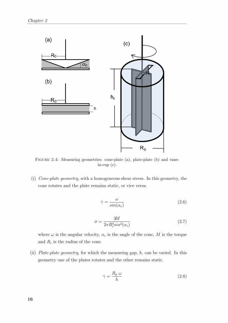
The measuring geometries used for performing the experiments shown in this thesis

are represented in Figure 2.4, for which the shear rate and the shear stress is

calculated according to the following equations [2–5]:

15

Chapter 2

Figure 2.4: Measuring geometries: cone-plate (a), plate-plate (b) and vane-in-cup (c).

(i) Cone-plate geometry, with a homogeneous shear stress. In this geometry, the

cone rotates and the plate remains static, or vice versa.

γ =ω

sin(αc)(2.6)

σ =3M

2πR3csin

2(αc)(2.7)

where ω is the angular velocity, αc is the angle of the cone, M is the torque

and Rc is the radius of the cone.

(ii) Plate-plate geometry, for which the measuring gap, h, can be varied. In this

geometry one of the plates rotates and the other remains static.

γ =Rp ω

h(2.8)

16

Experimental techniques and materials

σ =3 M

2πR3p

(1 + 1

3dlnMdlnω

) (2.9)

where Rp is the radius of the plate. The shear rate given by (2.8) represents

the shear rate at the rim, and this value is used for interpreting experimental

data for torsional flow [1].

(iii) Vane-in-cup geometry, in which the vane rotates and the cup remains static.

The material between the vanes moves as a solid block, making this geometry

similar to the Couette geometry (two concentric cylinders).

γ ≈ ω(Ri +Ro)/2

Ro −Ri

(2.10)

σ =M

2πhcR2i

(2.11)

where Ri is the radius of the vane, Ro is the radius of the cup and hc is the

length of the vane.

2.1.1.2 Rheological measurements

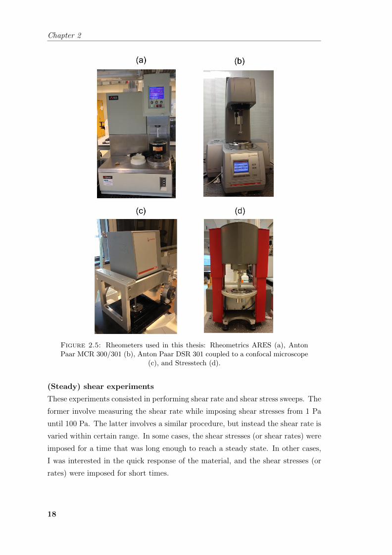
The rheological characterization of materials used in this thesis were performed

using the rheometers shown in Figure 2.5:

(i) Rheometrics ARES : a controlled-shear-rate rheometer, in which the the an-

gular velocity is imposed and the corresponding torque is measured.

(ii) Anton Paar MCR 300/301 and DSR 301 : controlled shear-stress rheometers;

in this case, the torque is imposed and the angular velocity is measured. The

DSR 301 rheometer was coupled to the confocal laser scanning microscope.

(iii) Stresstech: a controlled shear-stress rheometer.

Rheological measurements consisted of (steady) shear, viscosity bifurcation, oscil-

latory, creep, and stress growth experiments.

17

Chapter 2

Figure 2.5: Rheometers used in this thesis: Rheometrics ARES (a), AntonPaar MCR 300/301 (b), Anton Paar DSR 301 coupled to a confocal microscope

(c), and Stresstech (d).

(Steady) shear experiments

These experiments consisted in performing shear rate and shear stress sweeps. The

former involve measuring the shear rate while imposing shear stresses from 1 Pa

until 100 Pa. The latter involves a similar procedure, but instead the shear rate is

varied within certain range. In some cases, the shear stresses (or shear rates) were

imposed for a time that was long enough to reach a steady state. In other cases,

I was interested in the quick response of the material, and the shear stresses (or

rates) were imposed for short times.

18

Experimental techniques and materials

Viscosity bifurcation experiments

The viscosity bifurcation experiments consisted in imposing a shear stress and

measuring the evolution of the shear rate or the shear viscosity in time. These

experiments were useful for testing if a yield stress material is thixotropic or not.

For thixotropic materials if stresses below a critical value (σc) are imposed, then

the shear viscosity of the sample increases in time until the flow is halted together.

Conversely, at stresses only slightly above σc, the viscosity decreases with time to-

wards a low steady value. For non-thixotropic yield stress materials, as soon as a

stress above the yield stress is imposed, the material flows [6, 7].

Oscillatory measurements

These measurements consisted in imposing an oscillatory shearing, allowing the

determination of the storage (G′) and loss (G′′) moduli, of yield stress materials.

G′ is a measure of the storage of elastic energy, while G′′ is associated with the

viscous energy dissipated per cycle of deformation [3, 8].

Consider a sinusoidal shear strain γ of small amplitude γ0 and frequency ω, given

by γ = γ0 sinωt. The shear stress σ(t) produced by a small-amplitude deformation

is proportional to, but out of phase with γ:

σ(t) = σ0 sin(ωt+ δ) = γ0 [G′(ω)sin(ωt) +G′′(ω)cos(ωt)] (2.12)

where δ is the phase angle difference between the applied strain and the stress

response, and G′ is in phase with the strain and G′′ is in phase with the deformation

rate, γ.

For a perfectly elastic material, G′′ = 0 and δ = 0, whereas for a viscous fluid

G′ = 0 and δ = 90◦. In yield stress materials, both G′ and G′′ are nonzero and

0◦ < δ < 90◦.

Creep experiments

These measurements consisted in imposing a shear stress and recording the strain

response in time. At stresses lower than the yield stress, yield stress materials

behave like elastic solids, therefore the strain increases in time toward a constant

19

Chapter 2

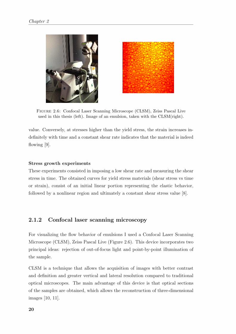
Figure 2.6: Confocal Laser Scanning Microscope (CLSM), Zeiss Pascal Liveused in this thesis (left). Image of an emulsion, taken with the CLSM(right).

value. Conversely, at stresses higher than the yield stress, the strain increases in-

definitely with time and a constant shear rate indicates that the material is indeed

flowing [9].

Stress growth experiments

These experiments consisted in imposing a low shear rate and measuring the shear

stress in time. The obtained curves for yield stress materials (shear stress vs time

or strain), consist of an initial linear portion representing the elastic behavior,

followed by a nonlinear region and ultimately a constant shear stress value [8].

2.1.2 Confocal laser scanning microscopy

For visualizing the flow behavior of emulsions I used a Confocal Laser Scanning

Microscope (CLSM), Zeiss Pascal Live (Figure 2.6). This device incorporates two

principal ideas: rejection of out-of-focus light and point-by-point illumination of

the sample.

CLSM is a technique that allows the acquisition of images with better contrast

and definition and greater vertical and lateral resolution compared to traditional

optical microscopes. The main advantage of this device is that optical sections

of the samples are obtained, which allows the reconstruction of three-dimensional

images [10, 11].

20

Experimental techniques and materials

This device was used for obtaining “movies” of flowing emulsions, from which it

was possible to reconstruct velocity profiles, showing the variation of the velocity

along the line perpendicular to the direction of the flow. For this aim, the CLSM

was coupled to the DSR 301 rheometer.

In addition, the CLSM was used for the observation of the interaction of emulsions

with different surfaces.

2.2 Materials

2.2.1 Emulsions

The emulsions used for this thesis are castor oil-in-water and silicone oil-in-water

emulsions. Both emulsions were stabilized using Sodium Dodecyl Sulfate (SDS,

from Sigma Aldrich), which is a surfactant molecule with the molecular formula:

CH3(CH2)11SO−4 Na

+. SDS is an anionic surfactant, as it dissociates to yield a

surfactant ion whose polar group is negatively charged [12].

2.2.1.1 Castor oil-in-water emulsion

Castor oil-in-water emulsions were prepared in the following way:

(i) Continuous phase: was prepared by dissolving SDS in ultra-pure water (Milli-

Q R©), obtaining a solution with 1 wt% SDS concentration.

(ii) Dispersed phase: consisting of Castor oil (Sigma-Aldrich).

(iii) Emulsification: the aqueous phase was added to the oil, subsequently both

phases were emulsified using a IKA T18 emulsifier at 24,000 rpm for 5 min-

utes. The internal volume fraction was φ = 0.8.

(iv) Emulsion with lower φ: were prepared by diluting the original emulsion

(φ = 0.80) with the 1 wt% SDS solution.

Thixotropic systems were prepared by manually mixing already-prepared emul-

sions with Bentonite clay (from Steetley bentonite & Absorbents Limited). The

21

Chapter 2

final clay concentration was 2 or 5 wt% with respect to the total amount of emul-

sion.

2.2.1.2 Silicone oil-in-water emulsion

Silicone oil-in-water transparent emulsions were prepared in the following way:

(i) Continuous phase: consisted of a solution of 46.2 wt% ultra-pure water (Milli-

Q R©) and 53.8 wt% glycerol (99 % GC, from Sigma-Aldrich). SDS (Sigma-

Aldrich) was disolved in the water-glycerol solution, in such a proportion

that the SDS concentration in the continuous phase was 1 wt%.

(ii) Dispersed phase: consisted of Silicone oil (Rhodorsil R©47 V 500); this phase

was dyed with Nile red (Sigma-Aldrich). For each 100 ml of oil, around 2 ml

of a saturated solution of Nile red dissolved in the oil were added.

(iii) Emulsification: the aqueous phase was added to the oil, subsequently both

phases were emulsified using a IKA T18 emulsifier at 24,000 rpm for 5 min-

utes. The internal volume fraction was φ = 0.8.

(iv) Centrifugation: in order to remove air bubbles from the samples, these were

centrifuged at 2,500 rpm for 30 minutes. The final system was a transparent

emulsion.

Thixotropic systems were prepared by adding Bentonite clay (from Steetley Ben-

tonite & Absorbents Limited) to the formulation before emulsification. The final

clay concentration was 1 or 3 wt% with respect to the total amount of emulsion.

2.2.2 Carbopol ‘gels’

Carbopol ‘gels’ were prepared by mixing Carbopol (Ultrez U10 grade) and ultra-

pure water for one hour, in such a proportion that the Carbopol concentration was

2 wt%. Sodium hydroxide (NaOH, from Sigma-Aldrich) was dissolved in water to

obtain a 18 wt% NaOH solution, which was used to adjust the pH of the carbopol-

water mixture to approximately 7: for each 500 g of carbopol-water mixture, 20 mL

of the 18 wt% NaOH solution were added. The resulting mixture was vigorously

22

Experimental techniques and materials

shaken and left to rest for one day. Samples with lower concentration of carbopol

were prepared by diluting the 2 wt% Carbopol sample with ultra-pure water.

2.2.3 Foam and hair gel

Foam used in this thesis is a commercially available foam (Gillette regular). Ad-

ditionally, hair gel is also commercially available (Albert Heijn), and basically is a

carbopol gel in which the pH is stabilized using triethanolamine instead of NaOH.

References

[1] H. A. Barnes, J. F. Hutton, and K. Walters, An Introduction to Rheology.

Elsevier Science Publishers B. V., 1989.

[2] C. W. Macosko, Rheology. Principles, measurements, and applications. Wiley

- VCH, New York, 1994.

[3] R. G. Larson, The Structure and Rheology of Complex Fluids. Oxford Uni-

versity Press, Inc., 1999.

[4] H. A. Barnes and Q. D. Nguyen, “Rotating vane rheometry—a review,” J.

Non-Newtonian Fluid Mech., vol. 98, pp. 1–14, 2001.

[5] P. Møller, Shear banding and the solid/liquid transition in yield stress fluids.

PhD thesis, Universite Paris 6 - Pierre et Marie Curie, 2008.

[6] P. Coussot, Q. D. Nguyen, H. T. Huynh, and D. Bonn, “Avalanche behavior

in yield stress fluids,” Phys. Rev. Lett., vol. 88, p. 175501, 2002.

[7] P. Coussot, Q. D. Nguyen, H. T. Huynh, and D. Bonn, “Viscosity bifurcation

in thixotropic, yielding fluids,” J. Rheol., vol. 46, pp. 573–589, 2002.

[8] Q. D. Nguyen and D. V. Boger, “Measuring the flow properties of yield stress

fluids,” Annu. Rev. Fluid Mech., vol. 24, pp. 47–88, 1992.

[9] P. C. F. Møller, A. Fall, and D. Bonn, “Origin of apparent viscosity in yield

stress fluids below yielding,” Europhys. Lett., vol. 87, p. 38004, 2009.

23

Chapter 2

[10] C. Sheppard and D. Shotton, Confocal laser scanning microscopy. BIOS

Scientific, 1997.

[11] S. J. Wright, V. E. Centonze, S. A. Stricker, P. J. D. vries, S. W. Paddock, and

G. Schatten, An Introduction to Confocal Microscopy and Three-Dimensional

Reconstruction, in: Methods in Cell Biology. Academic Press, Inc, 1993.

[12] L. L. Schramm, Emulsions, Foams, and Suspensions. Wiley - VCH Verlag

GmbH & Co. KGaA, Weinheim, 2005.

24