Using Vibration Analysis to Determine Refrigerant Levels in

an Automotive Air Conditioning System

Eric C. Stasiunas

Thesis submitted to the Faculty of the Virginia Polytechnic Institute and State University

in partial fulfillment of the requirements for the degree of

Master of Science in

Mechanical Engineering

Dr. Mary Kasarda, Chairman

Dr. Gordon Kirk

Dr. Al Wicks

June 20, 2002 Blacksburg, Virginia

Keywords: Vibration Analysis, Modal Analysis, Automotive Air Conditioning System

Copyright 2002, Eric Carl Stasiunas

ii

ABSTRACT

Using Vibration Analysis to Determine Refrigerant Levels In an Automotive Air Conditioning System

Eric C. Stasiunas Presently, auto manufacturers do not have do not have efficient or accurate methods to

determine the amount of refrigerant (R-134a) in an air conditioning system of an

automobile. In the research presented, vibration analysis is examined as a possible

method to determine this R-134a amount. Initial laboratory tests were completed and

experimental modal analysis methods were investigated. This approach is based on the

hypothesis that the natural frequency of the accumulator bottle is a function of the mass

of refrigerant in the system. Applying this theory to a working automotive air

conditioning bench test rig involved using the roving hammer method�forcing the

structure with an impact hammer at many different points and measuring the resulting

acceleration at one point on the structure. The measurements focused on finding the

natural frequency at the accumulator bottle of the air condition system with running and

non-running compressor scenarios. The experimental frequency response function (FRF)

results indicate distinct trends in the change of measured cylindrical natural frequencies

as a function of refrigerant level. Using the proposed modal analysis method, the R-134a

measurement accuracy is estimated at +3 oz of refrigerant in the running laboratory

system and an accuracy of +1 oz in the non-running laboratory system.

iii

To my family and friends

iv

ACKNOWLEDGEMENTS

I would first like to thank my advisor, Dr. Mary Kasarda, for taking a chance on a kid

from Tennessee. She has taught me how an engineer in the �real world� should handle

engineering problems because there are really are no answers in the back of the book. I

genuinely appreciate the guidance and support she has given me during my graduate

studies here at Virginia Tech.

I would also like to thank my committee members for the assistance they have given me

during the extent of the research. Dr. Gordon Kirk was always ready to lend his

experience and any encouragement. Dr. Al Wicks was always ready (if it wasn�t his tee

time) to lend a helping hand in figuring out what was going on with the accumulator in

the frequency domain. I enjoyed his classes immensely and am still learning more on the

subject of modal analysis every time I speak with him. I would also like to thank him for

showing me how cool modal analysis can be, and for all the Tennessee jokes that made

me laugh over the past year and a half. I thank all of y�all very much.

I would like to thank my family for being there every step of the way, even coming to

Virginia to see me defend my thesis. Mom and Dad, I am finally getting a job so there is

no need to worry about me anymore. My sister, Kelly, will have to come visit me out in

New Mexico when she gets an opening in her busy schedule. Oma and Opa, Grandma,

and Grandpa, I thank for everything they have taught me during my lifetime�from the

correct way to cook sauerkraut to how beautiful the state of Virginia is.

Finally, I would like to thank all of my friends for being there for me. I have some great

stories involving Rob Prins, Wojtek Krych, and Travis Bash. I thank Rob for being a

great friend and sharing his two lifetimes of experience with me concerning research,

jobs, and life in general. I thank Wojtek for making me laugh a lot, and for making me

realize there are worse things in life than screwing up on a math test. Travis was a

tremendous help with the modal testing and was always offering an encouraging word

when things would go awry in the testing and thesis phase of my graduate education. To

v

my girlfriend Karen Schafer, I sincerely thank her for her patience, encouragement, and

friendship during my time here at Virginia Tech.

Thanks to everyone. Eric C. Stasiunas Blacksburg, VA June, 2002

vi

TABLE OF CONTENTS

Abstract�������������������������������...ii

Acknowledgments���������������������������..iv

List of Figures����������������������������...viii

List of Tables�����������������������������...x

Nomenclature�����������������������������..xi

1 Introduction����������������������������� 1

1.1 General Overview�����������������������. 1

1.2 Motivation��������������������������. 2

1.3 Current Refrigerant Measurement Methods�������������. 3

1.4 Literature Review�����������������������. 5

2 Vibration and Modal Analysis Background���������������� 8

2.1 Modal Analysis General Overview����������������... 8

2.2 Vibration Theory����������������.�������.. 9

2.3 Modal Theory����������������.��������...12

2.4 Experimental Modal Analysis����������������.��.. 15

2.5 Digital Signal Processing����������������.����. 17

3 Automobile Air Conditioning Background����������������. 20

4 Experimental Setup and Procedure����������������.��� 22

4.1 Laboratory Test Rig����������������.������. 22

4.2 Experimental Setup����������������.������.. 30

4.3 Experimental Procedure����������������.����... 32

5 Frequency Response Analysis (Results) ����������������.�. 36

5.1 General Overview����������������.������� 36

5.2 Mode Shapes of the Accumulator Bottle��������������.. 36

vii

5.3 Cantilever Natural Frequency�����������..��.����... 38

5.3.1 Effects of Accumulator Clamp Tightness����������.. 41

5.4 Cylindrical Natural Frequency�����������������..... 43

5.4.1 Effects of Accelerometer Placement��..���.������.. 47

5.4.2 Effects of Dashboard Controller Settings����������.. 49

5.4.3 Time Transient Tests����������������.��.53

5.4.4 Non-running System Tests����������������. 56

6 Conclusions and Future Work����������������.����� 60

6.1 Overview of Work Completed����������������.��. 60

6.2 Discussion of Results����������������.�����... 61

6.3 Conclusions����������������.���������.. 67

6.4 Future Work����������������.���������. 68

References����������������.���������������. 69

Appendix A � Air Conditioning System Test Conditions�����..�������... 70

Appendix B � Frequency Response Functions Data���������������.. 72

Appendix C � Analytical Natural Frequencies of the Accumulator���������.. 76

C.1 Analytical Natural Frequencies���������������... 76

C.2 Cantilever Natural Frequencies���������������... 76

C.3 Cylindrical Natural Frequencies���������������..79

Vita����������������������������������. 83

viii

LIST OF FIGURES

Number Title Page

1-1 Automobile assembly line 2

1-2 Sight glass assembly 3

1-3 Manifold pressure gage set 4

2-1 An ideal system model 9

2-2 Modes of a cantilevered beam 11

2-3 Graphical example of an FRF 14

2-4 Impact hammer, accelerometer, and signal analyzer 16

2-5 Roving hammer method 16

2-6 Autospectrum of impact hammer hit 17

2-7 Coherence plot 18

2-8 Relationship between autospectrum and coherence 19

3-1 Accumulator/orifice tube automotive air conditioning system 20

4-1 Laboratory test rig (air conditioning system) 23

4-2 Schematic of laboratory test rig 23

4-3 A/C compressor and DC motor 24

4-4 Condenser, radiator, and fan 25

4-5 Dashboard unit, controller, and ductwork 26

4-6 Dashboard controller 27

4-7 Accumulator bottle 28

4-8 Refrigerant management system 29

4-9 Modal testing setup 30

4-10 Autospectrum of different hammer tips 31

4-11 Auxiliary system of laboratory test rig 33

4-12 Performance of modal test 34

5-1 Cantilever mode shape of the accumulator bottle 37

5-2 Studied modes of accumulator bottle 38

5-3 FRF of cantilever natural frequencies for various R-134a levels 39

ix

5-4 Cantilever natural frequency vs. R-134a level in running system 40

5-5 Clamp tightness effects on cantilever natural frequency 42

5-6 Cantilever natural frequency vs. bolt tightness 43

5-7 FRF plot of cylindrical natural frequencies for various R-134a levels 44

5-8 Autospectrum of impact hammer 45

5-9 Cylindrical natural frequency vs. R-134a level in running system 46

5-10 Location effect of accelerometer on cylindrical mode 48

5-11 FRF of new accelerometer placement for various R-134a levels 49

5-12 Dashboard controller settings tested 50

5-13 FRF of various temperature control settings (10.50 ounces) 51

5-14 FRF of various temperature control settings (15.50 ounces) 51

5-15 FRF of various temperature control settings (20.00 ounces) 52

5-16 Transient test of 20.00 ounce R-134a charge 54

5-17 Transient test of 10.25 ounce R-134a charge 55

5-18 FRF plot of cylindrical natural frequencies for various R-134a levels 56

5-19 Cylindrical natural frequency vs. R-134a level in non-running system 58

B-1 Test setup for determining cylindrical mode 73

B-2 Frequency response function for side A 74

B-3 Frequency response function for side C 74

B-4 Frequency response function for side F 74

B-5 Determined cylindrical mode of accumulator 75

C-1 Beam with tip mass in transverse vibration 77

C-2 Dimensions of inlet line used to calculate first natural frequency 78

C-3 Modes of a cylinder analyzed in the analysis 80

C-4 Axial and circumferential modes 81

x

LIST OF TABLES

Number Title Page

5-1 Natural frequencies (Hz) for varying levels of R-134a (cantilever mode) 40

5-2 Natural Frequencies (Hz) for varying levels of R-134a (cylindrical mode) 46

5-3 Temperatures for varying thermostat settings 52

5-4 Variation of natural frequency with dashboard settings 53

5-5 Natural frequencies for varying levels of R-134a

(30 minutes after shutoff) 58

A-1 Running system tests (cylindrical natural frequency) 70

A-2 Non-running system tests (cylindrical natural frequency) 71

A-3 Running system tests (cantilever natural frequency) 71

C-1 First natural frequency calculations (beam with tip mass) 79

C-2 Analytical natural frequencies for cylindrical modes 81

NOMENCLATURE

Symbol Metric Units Description

c kg/sec Damping Coefficient

F N Input of System (Force)

g Forcing Location

H m/(sec2 N) Frequency Response Function of a System

(Transfer Function)

i Response Location

K N/m Stiffness Matrix

k N/m Stiffness

M kg Mass Matrix

m kg Mass

N Degrees of Freedom

n Natural Frequency Number

t sec Time

u Vector of Constants

X&& m/sec2 Output of a System (Acceleration)

x m Displacement Vector

x&& m/sec2 Acceleration Vector

φ Mode Vector

θ rad Phase

ζ Damping ratio

ω rad/sec Frequency

ωn rad/sec Natural Frequency

xi

Chapter 1

Introduction and Literature Review

1.1 General Overview

Vibration analysis has been used successfully in the engineering field for

measuring dynamic characteristics in mechanical structures and systems. This thesis

incorporates vibration analysis into automotive applications for the purpose of

performing a non-destructive evaluation of refrigeration level in automotive air

conditioners. The theory behind the vibration analysis is based on the theory that the

natural frequencies of systems are a function of mass. In the case of an automotive air

conditioner, the level of refrigerant contributes to the mass of the system, which is

reflected in the natural frequency. Each natural frequency has a corresponding mode

shape. Mode shapes, or modes, are the relative displacements of the system’s masses

while vibrating at that particular natural frequency. Natural frequencies and mode shapes

are discussed in further detail in Chapter 2.

The type of vibration analysis performed on the automotive air conditioner in the

presented research is modal analysis. Modal analysis is an experimental procedure that

uses transfer functions, which measure the response of a system from a known input, to

obtain the dynamic characteristics of structures and systems. Modal analysis is used to

both verify analytical models developed for systems and to determine parameters for

input into the system models for analysis.

In this work, the modal analysis technique was used in a laboratory test rig that

was built to simulate a working automobile air conditioner. Testing focused on the

accumulator bottle of the air conditioning system, because of the high concentration of

refrigerant contained within. Refrigerant R-134a was the refrigerant used in the test rig,

and the level of the refrigerant in the system was varied using a refrigerant management

system. Tests were performed with running and non-running scenarios. Several

1

parameters were studied as well: accumulator bottle clamp tightness, accelerometer

placement, dashboard control settings, transient testing, and non-running system testing.

1.2 Motivation

Automobile manufactures are concerned with the goal of improving the quality

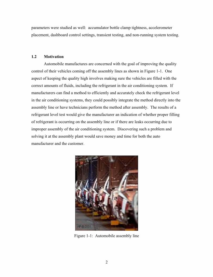
control of their vehicles coming off the assembly lines as shown in Figure 1-1. One

aspect of keeping the quality high involves making sure the vehicles are filled with the

correct amounts of fluids, including the refrigerant in the air conditioning system. If

manufacturers can find a method to efficiently and accurately check the refrigerant level

in the air conditioning systems, they could possibly integrate the method directly into the

assembly line or have technicians perform the method after assembly. The results of a

refrigerant level test would give the manufacturer an indication of whether proper filling

of refrigerant is occurring on the assembly line or if there are leaks occurring due to

improper assembly of the air conditioning system. Discovering such a problem and

solving it at the assembly plant would save money and time for both the auto

manufacturer and the customer.

Figure 1-1: Automobile assembly line

2

Along with improving the quality control at automotive assembly plants, an

inexpensive and accurate method of measuring automobile refrigerant levels could be

used at the automotive dealership when problems arise with the air conditioning unit or

during normal maintenance checks. Depending on the level of refrigerant measured, the

specialist could determine if there is a leak, and the system could be thoroughly checked.

This early detection of refrigerant leaks has the added benefit of preventing further

refrigerant loss into the atmosphere, which would result in cleaner air and a less polluted

environment.

1.3 Current Refrigerant Measurement Methods

Current methods available to measure refrigerant levels in automotive air

conditioning systems are not very accurate or efficient. Such methods include viewing

the refrigerant with a sight glass, measuring the output vent temperature with a

thermometer, and measuring the system pressure with a manifold gage set. Automobile

manufacturer recommendations usually determine which methods are used.

Some automobile air conditioning systems contain a sight glass located in the

refrigeration line that allows for a real-time inspection of the refrigerant in the system. A

sight glass for a refrigeration system can be seen in Figure 1-2. The appearance and the

consistency (clear, bubbles present) of the refrigerant give only an indication of an

overcharge or undercharge of refrigerant in the system. Used for a preliminary check, the

sight glass does not give an accurate indication of refrigerant level [Crouse, 1977].

Figure 1-2: Sight glass assembly [Eclipse Holdings, 2002]

Measuring the temperature of the air leaving the air conditioning outlet in the

vehicle is another method used to determine the amount of refrigerant in the system. If

3

the outlet temperature is within a certain temperature range, it is assumed there is a

correct amount of refrigerant in the system. Temperatures that are under the temperature

range indicate an undercharge of refrigerant in the system. This method is sometimes

used with the manifold pressure gage set method to get a better idea of the refrigerant

charge in the system [Crouse, 1977].

Manifold pressure gage sets, as shown in Figure 1-3, consist of a low-pressure

and a high-pressure gage that measure the low and high-pressure side of the air

conditioning system, respectively. The measured pressures of a running system can be

used with the manufacturer’s operating specifications to determine if an under- or

overcharge exists in the system. Ambient temperatures and humidity must be taken into

account when using the pressure gages to determine refrigerant level. If it is a

particularly hot or humid day, the air conditioner must work harder to cool the air,

resulting in higher measured pressures than normal. Again, this method can only

determine if the system is under or over charged, not an exact amount [Crouse, 1977].

Figure 1-3: Manifold pressure gage set [White Industries, 2002]

The most accurate way to measure the refrigerant in an automobile air

conditioning system is also the most time consuming. Using a refrigerant management

system, the refrigerant can be vacuumed out of the air conditioner entirely and weighed.

This method is inefficient, since it requires that all of the refrigerant must be vacuumed

out of the system. From actual testing experience, this process may take anywhere from

30 minutes to an hour to complete.

4

1.4 Literature Review

Over the past decade, researchers have performed experimental vibration analysis

of different containers with varying levels of fluids and solids. Mourad and Haroun

[1990] were interested in the vibration response of cylindrical liquid-filled tanks due to

transient loading. The test specimen used was a steel cylindrical tank 132 inches high, 48

inches in diameter, and 0.08 inches thick. To simulate simple supported and free edge

boundary conditions, the tank was tested with and without its removable conical cover.

The input vibrations of 0 to 50 Hz were provided with a 10-pound shaker that was

connected to a push-rod (stinger) and a force transducer. The response was measured

with 12 accelerometers placed circumferentially and 3 accelerometers placed axially on

the cylinder. Three liquid levels in the tank—empty, half-full, and full—were examined

in the research.

Test results revealed that as the liquid level in the tank increased, the resulting

response decreased in magnitude and the natural frequencies decreased as well (due to an

increase in mass). This trend was evident in both uncovered and covered cylinder tests,

with the natural frequencies for the uncovered cylinder being higher than the covered

cylinder because the cover adds more mass than stiffness to the structure. Increasing the

liquid levels resulted in better-defined mode shapes. Local modes were also discovered

for the various liquid levels tested. A local mode is identified by peaks, indicating

natural frequencies, in only one or two measured frequency response functions with no

corresponding peaks in the rest [Mourad and Haroun, 1990].

A year later, Mourad and Haroun [1991] repeated the vibration response tests

using the same liquid levels (empty, half-full, full) with a different steel tank. The

dimensions of this tank were 4 feet (48 inches) high, 8 feet (96 inches) in diameter, and

0.08 inches thick; much broader than the tank used in the earlier experiment. The input

vibrations of 0 to 125 Hz were provided with a 30-pound shaker placed on the cover of

the structure. Measuring the input required an accelerometer and the response was

measured with 24 accelerometers placed circumferentially and 4 accelerometers placed

axially on the cylinder.

The results from the test of a broad cylindrical tank were similar to the results of

the taller cylindrical tank tested earlier. The modes decreased in magnitude, the natural

5

frequency values decreased, and the modes were better defined as the liquid level was

increased in the tank. Again, local modes were observed throughout the range of

frequencies tested [Mourad and Haroun, 1991].

Tranxuan [1997] performed experimental vibration analysis on thin-walled

structures to determine how the mass of granular and liquid bulk material contained

within would affect the structures’ dynamic characteristics. Motivation for the research

resulted from the fact that thin-walled structures are commonly used to store and

transport bulk materials and the desire to understand the response of these structures due

to their use in land and sea transportation. An open-top rectangular steel tank of

dimensions 350 mm (13.8 inches) wide, 400 mm (15.7 inches) tall, and 550 mm (21.7

inches) long was analyzed with varying amounts of bulk material of liquid and granular

forms. The loads of the bulk material tested were from 0 kg to 30 kg in steps of 5 kg,

with the types tested being water, motor oil, oats, sand, and finely crushed rock. An

impact hammer was used as an input device with several accelerometers measuring the

response in the frequency range of 0 to 200 Hz.

Results from the experimental analysis of the rectangular tank demonstrated the

natural frequency for a particular mode shape is affected by the mass of the bulk material

and the type of the bulk material itself. There were two factors affecting the change in

natural frequency: the added-mass effect (decreasing the natural frequency) and the

added-stiffness effect (increasing the natural frequency). Determining which was more

pronounced depended on the relative stiffness of the bulk material compared with the thin

walled structure. For example, water and motor oil were far less stiff compared to the

thin walls of the structure and the added-mass effect was more pronounced, always

resulting in lower natural frequencies when the amount of liquid was increased.

However, the granular materials tested—sand, finely crushed rocks, and oats—behaved

differently. For small amounts of granular material, a decrease in the natural frequencies

occurred, indicating an added-mass effect in the system. When large amounts of the

granular material were added to the structure, the natural frequencies of the system would

increase, indicating a more pronounced added-stiffness effect present in the system.

Results of the experimental analysis also revealed local modes present with an increase of

all types of bulk material tested [Tranxuan, 1997].

6

The previous vibration experiments on containers with varying levels of fluid all

contain the same general results. The natural frequencies of the containers decrease as

the liquid levels increase, due to the added mass in the system. Local modes (modes that

were present at some liquid levels and not others) were also discovered. These results

indicate it is reasonable to theorize that as refrigerant level in the accumulator bottle

increases, the natural frequency should decrease in a measurable way. This literature

review also helps in interpreting and understanding the resulting data from the research

presented in this thesis.

7

Chapter 2

Vibration and Modal Analysis Background

The goal of the research presented in this theis is to measure refrigerant levels

using vibration analysis. The type of vibration analysis applied to the research is modal

analysis. To understand what modal analysis is and how it works, a general overview

and some aspects of modal analysis is covered are this chapter. The aspects include the

following: vibration theory, modal theory, experimental modal analysis, and some

features of digital signal processing. Because an automotive air conditioning system is

being tested, a brief review of an air conditioning system is included as well.

2.1 Modal Analysis General Overview

Modal analysis is a form of vibration analysis commonly used to examine the

dynamic characteristics of vibrating systems. The specific characteristics investigated in

this research were the natural frequencies and mode shapes of the system. Natural

frequencies are the frequencies at which the system exhibits resonance, and mode shapes

are the relative displacements of the system’s masses when excited at these natural

frequencies. Both the natural frequencies and mode shapes can be obtained from the

direct result of the modal analysis—the frequency response function (FRF).

The FRF is a transfer function that relates the output to the input of a system in

the frequency domain. A model for an ideal system with a transfer function H(ω), input

F(ω), and output X(ω), can be seen in Figure 2-1. For the research presented in this

thesis, the input is the forcing function used to excite the system, and the output is the

resulting acceleration of the system.

8

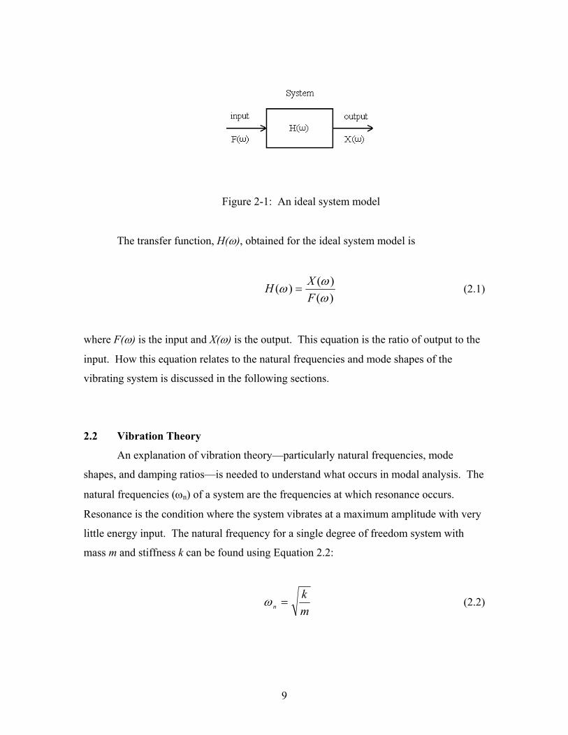
Figure 2-1: An ideal system model

The transfer function, H(ω), obtained for the ideal system model is

)()()(

ωωω

FXH = (2.1)

where F(ω) is the input and X(ω) is the output. This equation is the ratio of output to the

input. How this equation relates to the natural frequencies and mode shapes of the

vibrating system is discussed in the following sections.

2.2 Vibration Theory

An explanation of vibration theory—particularly natural frequencies, mode

shapes, and damping ratios—is needed to understand what occurs in modal analysis. The

natural frequencies (ωn) of a system are the frequencies at which resonance occurs.

Resonance is the condition where the system vibrates at a maximum amplitude with very

little energy input. The natural frequency for a single degree of freedom system with

mass m and stiffness k can be found using Equation 2.2:

mk

n =ω (2.2)

9

A single degree of freedom system is the simplest model used to analyze vibrating

systems. In realistic situations, multiple degree of freedom (MDOF) systems are used for

the analytical model. If a system has N degrees of freedom, it also has N natural

frequencies. Most systems contain an infinite number of natural frequencies, but only the

first few are of realistic concern and are analyzed.

Analytically finding the natural frequencies of an undamped N degree of freedom

system involves first finding the system’s N governing equations of motion. The

equations of motion are then written in matrix form, resulting in N×N mass (M) and

stiffness (K) matrices that are respectively multiplied by the acceleration and

displacement vectors as shown in Equation 2.3.

0xx =+ KM && (2.3)

This equation can be solved assuming a harmonic solution of the form ,

where u is a vector of constants, and ω is a frequency constant to be determined.

Substituting the assumed solution into Equation 2.3, integrating where necessary, and

collecting terms results in

tjet ωux =)(

( ) 0u =+− KM2ω (2.4)

Equation 2.4 is an example of the generalized eigenvalue problem and the values of ω

can be solved for by using typical eigenvalue methods. The solution for the discussed

undamped system can be found by finding the determinant of the coefficient

matrix, . Solving for the determinant results in the characteristic equation

of the system, and from this characteristic equation, the system’s N natural frequencies

can be found. There will be N positive solutions for ω, each of them a system natural

frequency. The mathematical process used to find natural frequencies for more complex

systems involving damping and forced response is somewhat similar to the discussed

method and is given in further detail in Inman [2001] and Ewins [2000].

( KM +− 2ω )

10

Mode shapes, or modes, are the relative displacements of the system’s masses

when vibrating at a natural frequency. Each mode shape of a system corresponds to a

particular natural frequency—therefore, for N natural frequencies, there are N mode

shapes. The first two mode shapes for the transverse vibration of a cantilevered beam of

length L can be seen in Figure 2-2. The y-axis is the axis of vibration and displacement,

and the x-axis is the length of the beam. Dashed lines on the mode plots represent the

beam at rest.

Figure 2-2: Modes of a cantilevered beam: (a) orientation (b) mode 1 (c) mode 2

The modes in Figure 2-2 would occur at their respective natural frequencies:

mode 1 at ω1 and mode 2 at ω2. The displacement magnitudes are relative and

mathematically normalized; although for this research, they were not. The mode shapes

presented in this research were used only as a reference to determine which natural

frequency was being examined.

Although the damping ratio (ζ) was not examined in the research presented, it is

useful to understand what the damping ratio is and how it relates to the system mass and

spring stiffness. The equation for the non-dimensional damping ratio for a SDOF system

can be calculated using

kmc

2=ζ (2.5)

where k is the spring stiffness, m is the system mass, and c is the damping coefficient of

the system which can be calculated mathematically or found experimentally. The

damping ratio can be any positive value and represents how well a system is damped.

11

When ζ is equal to 0, the system is defined as being undamped, when ζ is equal to 1, the

system is defined as critically damped, and when ζ is greater than 1, the system is defined

as overdamped. A system is underdamped when ζ is less than the critically damped

condition (0<ζ<1). As a system transitions from an undamped system to a critically

damped system, the amplitude of the response becomes less pronounced, and the phase

change (which will be discussed later) is less abrupt. In a MDOF system, when there are

N degrees of freedom, there are N damping ratios, each corresponding to a natural

frequency. The damping ratio is used in the mathematical modal analysis (frequency

response function) equation and it is important to note that the system mass and stiffness

is contained within this equation.

2.3 Modal Theory

The modal theory expands upon the vibration theory discussed previously. For a

single degree of freedom system (a system with one mass moving along one axis) the

forced frequency response function is

nn jFXH

ζωωωωω

ωωω

2)()()( 22

2

++−−==

&& (2.6)

where ωn is the system’s natural frequency, ω is the forcing (driving or applied)

frequency, and ζ is the damping ratio. Equation 2.6 can be derived using Newton’s

second law (sum of the forces equals the mass multiplied by acceleration) on the

vibrating system and solved assuming a solution containing complex variables.

For a system containing N degrees of freedom with a single forcing function at

location g and a response measured at location i, the single degree of freedom system can

be expanded into the forced frequency response function equation:

( )( )[ ]∑

= ++−−==

N

n nnn

gnin

g

iig MjF

XH1

22

2

2)()()(

ζωωωωωφφ

ωωω

&& (2.7)

12

where φ are the mode vectors at i and g, ωn is the natural frequency, ω is the forcing

(driving) frequency, ζ is the damping ratio, and Mn is the modal mass. Further details of

the previous equations and the derivation process can be found in Ewins [2000]. Both

Equation 2.6 and Equation 2.7 are complex valued—they contain real and imaginary

components. The magnitude ( )(ωH ) and phase (θ) information between the input and

output can be extracted from Equation 2.7 using the following equations:

( )( )[ ]∑

= ++−=

N

n nnn

gninig

MH

12222

2

)2()()(

ζωωωω

ωφφω (2.6)

( )( )[ ]∑

=

−

+−=

N

n nn

gninn

M122

21

)(2

tanωω

ωφφζωωθ (2.7)

From these equations, it can be shown that as the forcing frequency approaches the

natural frequency, the magnitude of the FRF increases, and the phase begins to shift

toward ±90 degrees. Once the two frequencies are equal (ωn = ω), the magnitude has

reached its peak and the phase is ±90 degrees. As the forcing frequency leaves the

natural frequency, the magnitude decreases and the phase completes a ±180 degree shift.

The direction of the phase (+ or −) is determined from the signs (+ or −) of the mode

vectors (φ) in the frequency response function equation.

Frequency response functions are typically plotted two ways: as a log-magnitude

versus frequency plot and a phase versus frequency plot. An example of a graphical FRF

is shown in Figure 2-3.

13

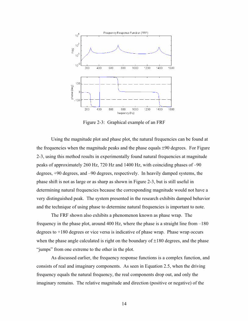
Figure 2-3: Graphical example of an FRF

Using the magnitude plot and phase plot, the natural frequencies can be found at

the frequencies when the magnitude peaks and the phase equals ±90 degrees. For Figure

2-3, using this method results in experimentally found natural frequencies at magnitude

peaks of approximately 260 Hz, 720 Hz and 1400 Hz, with coinciding phases of –90

degrees, +90 degrees, and –90 degrees, respectively. In heavily damped systems, the

phase shift is not as large or as sharp as shown in Figure 2-3, but is still useful in

determining natural frequencies because the corresponding magnitude would not have a

very distinguished peak. The system presented in the research exhibits damped behavior

and the technique of using phase to determine natural frequencies is important to note.

The FRF shown also exhibits a phenomenon known as phase wrap. The

frequency in the phase plot, around 400 Hz, where the phase is a straight line from –180

degrees to +180 degrees or vice versa is indicative of phase wrap. Phase wrap occurs

when the phase angle calculated is right on the boundary of ±180 degrees, and the phase

“jumps” from one extreme to the other in the plot.

As discussed earlier, the frequency response functions is a complex function, and

consists of real and imaginary components. As seen in Equation 2.5, when the driving

frequency equals the natural frequency, the real components drop out, and only the

imaginary remains. The relative magnitude and direction (positive or negative) of the

14

imaginary components at the natural frequencies can be used to plot the mode shapes of

the structure, as FRFs are calculated along the test structure.

2.4 Experimental Modal Analysis

Natural frequencies and modes shapes can be determined experimentally using

modal analysis. To perform this experimental analysis, three actions are required: the

system needs to be excited, the response of the system needs to be measured, and the

resulting data needs to be analyzed in the frequency domain.

The research presented involved an impact hammer to excite the system, an

accelerometer to measure the response, and a Hewlett-Packard digital signal analyzer to

analyze the data in the frequency domain. These components can be seen in Figure 2-4.

Impact hammers provide a quick and easy way to excite systems over a broad range of

frequencies. Containing a force transducer in the tip, the impact hammer allows for the

measurement of the amount of force put into the system. The tip of the impact hammer

can be exchanged between different materials differing in stiffness. The different

hammer tips used determine what frequency range will be measured and what the input

power will be. The concepts of input power will be discussed further in the next section,

and the difference in hammer tips will be discussed further in the Chapter 4. For this

research, a plastic tip and a steel hammer tip were used. Accelerometers measure the

response of the system due to the input force applied. The input (force) and output

(acceleration) are measured and recorded using the digital signal analyzer. Converting

the measured data from the time domain into the frequency domain allows the signal

analyzer to display the Frequency Response Function (FRF), the power spectrum, and the

coherence function.

15

Figure 2-4: Impact hammer, accelerometer, and signal analyzer

The particular name given to the method of testing performed in this research

with the hardware used (impact hammer and accelerometer) is the roving-hammer

method. In this method, the accelerometer is placed in one location of a structure and the

impact hammer is used to excite the system in many different test points on the system,

thus roving over the test piece. Figure 2-5 illustrates an example of a roving hammer

method performed on a cantilevered beam.

Figure 2-5: Roving hammer method

16

2.5 Digital Signal Processing

In performing experimental modal analysis, some knowledge of digital signal

processing is necessary. Two important concepts used to obtain valid results from modal

testing are the power spectrum, and the coherence function. Both of these processes are

performed by and displayed on the HP digital signal analyzer in the presented research.

The autospectrum is used to find the “power” of a signal, such as the measured

force and acceleration performed in the research. By definition, the autospectrum is the

Fourier transform of the autocorrelation function, which will not be discussed in detail

because they were not analyzed during testing. Much like the FRF, the autospectrum is

plotted with frequency versus magnitude in decibels (dB). However, the autospectrum is

a real valued function that does not contain any phase information. A sample plot of an

autospectrum from an impact-hammer hit is shown in Figure 2-6. When exciting a

system, it is important to put as much energy into the system as necessary in order for the

response transducer to “pick up” this energy and respond accordingly. Dips that occur in

the autospectrum indicate very little energy as shown in the figure at approximately 2700

Hz.

Figure 2-6: Autospectrum of impact hammer hit

17

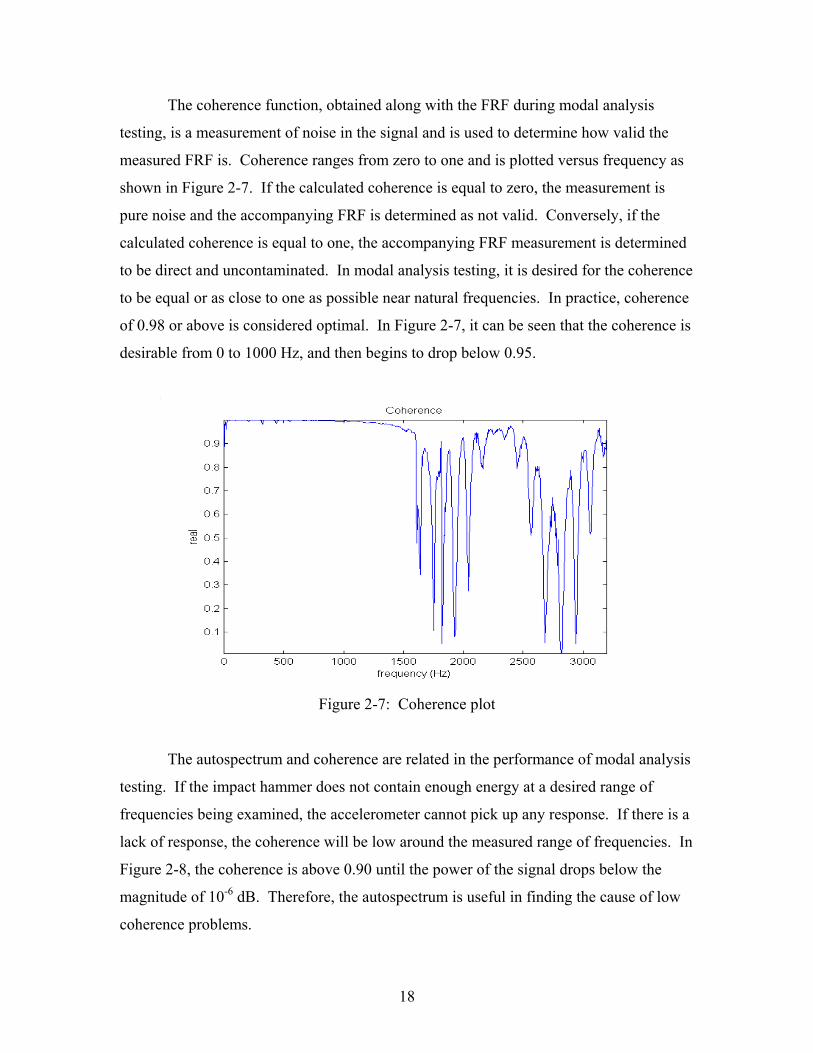
The coherence function, obtained along with the FRF during modal analysis

testing, is a measurement of noise in the signal and is used to determine how valid the

measured FRF is. Coherence ranges from zero to one and is plotted versus frequency as

shown in Figure 2-7. If the calculated coherence is equal to zero, the measurement is

pure noise and the accompanying FRF is determined as not valid. Conversely, if the

calculated coherence is equal to one, the accompanying FRF measurement is determined

to be direct and uncontaminated. In modal analysis testing, it is desired for the coherence

to be equal or as close to one as possible near natural frequencies. In practice, coherence

of 0.98 or above is considered optimal. In Figure 2-7, it can be seen that the coherence is

desirable from 0 to 1000 Hz, and then begins to drop below 0.95.

Figure 2-7: Coherence plot

The autospectrum and coherence are related in the performance of modal analysis

testing. If the impact hammer does not contain enough energy at a desired range of

frequencies being examined, the accelerometer cannot pick up any response. If there is a

lack of response, the coherence will be low around the measured range of frequencies. In

Figure 2-8, the coherence is above 0.90 until the power of the signal drops below the

magnitude of 10-6 dB. Therefore, the autospectrum is useful in finding the cause of low

coherence problems.

18

Figure 2-8: Relationship between autospectrum and coherence

The final aspect of digital signal processing used in the presented research is the

averaging process used to obtain the recorded FRFs. Averaging is used in vibration

analysis to provide data with a greater accuracy and reliability, resulting in a higher

coherence, than if just one measurement were to occur. Random vibration testing

involves taking many averages, anywhere from one to an infinite amount. For typical

impact hammer testing, the input into the system is not a random vibration; therefore,

fewer averages are needed for accurate results. For the presented research, three averages

were performed for each measured frequency response function.

19

Chapter 3

Automotive Air Conditioning Background

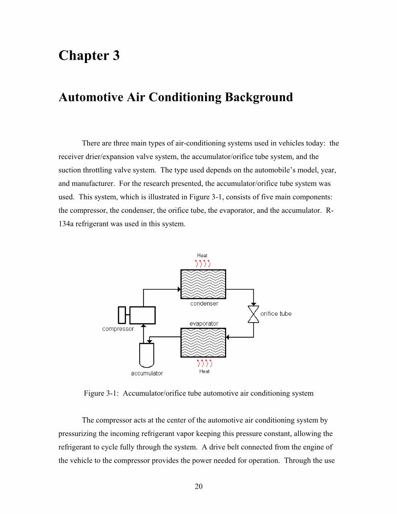
There are three main types of air-conditioning systems used in vehicles today: the

receiver drier/expansion valve system, the accumulator/orifice tube system, and the

suction throttling valve system. The type used depends on the automobile’s model, year,

and manufacturer. For the research presented, the accumulator/orifice tube system was

used. This system, which is illustrated in Figure 3-1, consists of five main components:

the compressor, the condenser, the orifice tube, the evaporator, and the accumulator. R-

134a refrigerant was used in this system.

Figure 3-1: Accumulator/orifice tube automotive air conditioning system

The compressor acts at the center of the automotive air conditioning system by

pressurizing the incoming refrigerant vapor keeping this pressure constant, allowing the

refrigerant to cycle fully through the system. A drive belt connected from the engine of

the vehicle to the compressor provides the power needed for operation. Through the use

20

of a magnetic clutch, the compressor is regulated between an on and off position

depending on system pressures (too high or too low) or desired selections on the

passenger dashboard controller. Activating the clutch sends the refrigerant vapor into the

condenser.

The condenser is a heat exchanger that uses coils to remove heat from the

refrigerant. Due to the compression process, the compressed vapor that enters the

condenser is very hot. Blowing air through the condenser coils causes the refrigerant

vapor to condense into a liquid. A liquid at this point, the refrigerant is sent from the

condenser into an orifice tube.

The orifice tube is the dividing element between the high and low-pressure sides

of the system and usually contains a filter on both ends to capture debris that forms in the

system. Since the orifice tube is a fixed size, the magnetic compressor clutch controls

refrigerant flow through the orifice by engaging or disengaging, depending on the

pressure in the air conditioning lines. Once the liquid refrigerant passes through the

orifice tube, it enters the evaporator.

The evaporator is a heat exchanger that uses coils to remove heat from the

surrounding air. Since the evaporator is located inside, or adjacent to, the passenger

compartment of the automobile, the heat removed is the heat inside the vehicle. The air

that is blown through the evaporator and into the passenger compartment is cold for this

reason, the air contains very little heat. The heat removed from the air is absorbed into

the liquid refrigerant and causes the refrigerant to boil into a vapor or vapor/liquid

mixture, which is then sent to the accumulator.

The refrigerant entering the accumulator may be a vapor or vapor/liquid mixture,

depending on system pressures or passenger dashboard controller settings. Since gas

compressors are damaged if liquids are introduced, a device is needed to allow the

introduction of vapor, but not liquids, into the compressor. The accumulator

accomplishes this goal by storing the refrigerant mixture and allowing only the vapor to

exit by the use of a standpipe or gravity. A desiccant bag is typically placed into the

accumulator to absorb any damaging moisture that may have gotten into the air

conditioning system during assembly or servicing. The refrigerant vapor that exits the

accumulator is then sent to the compressor, and the cycle is repeated.

21

Chapter 4

Experimental Setup and Procedure

The accumulator was the chosen location for modal testing in the research

presented. In an automotive air-conditioning system, the accumulator is where the

concentration of R-134a would be at its greatest, and would likely give a larger response

difference between refrigerant levels than anywhere else in the system. The accumulator

bottle was tested using a laboratory test rig with the experimental setup and procedure

that follows.

4.1 Laboratory Test Rig

Examination of the theory that the natural frequency of the accumulator bottle

was a function of the refrigerant level in the automobile air conditioning system first

required the construction of a laboratory test rig. This rig was to mimic the functions of

an actual automobile air conditioning system by operating at engine idle compressor

speeds and providing all of the settings available on the dashboard controller—full air

temperature range and four blower settings. All of the components used to build the rig

were from a particular vehicle (actual model of vehicle is proprietary information). The

laboratory test rig, along with associated hardware necessary to operate the system, is

shown in Figure 4-1.

22

Figure 4-1: Laboratory test rig (air conditioning system)

A schematic depicting the laboratory test rig can be seen in Figure 4-2. The

laboratory test rig required many different components to reproduce an actual vehicle’s

air conditioning system. The different systems (refrigerant, electric, water, air) can be

seen in the figure and are discussed in further detail.

Figure 4-2: Schematic of laboratory test rig

23

Running the air conditioning (AC) compressor required the use of a variable

speed direct current (DC) motor as shown in Figure 4-3. The compressor speed was

measured using a stroboscope and was run at the particular engine idle speed of 1010

rpm, which was determined from the model and type of vehicle from which the

components of the test rig originates from. During testing, however, the compressor

speed tended to gradually increase from the set idle running speed of 1010 rpm up to

1100 rpm due to unreliable motor speed control.

Figure 4-3: A/C compressor and DC motor

The compressor contained a magnetic clutch that was operated from the

dashboard controller. When the air conditioning setting was selected on this controller,

the compressor clutch was activated, and the refrigerant would be cycled through the

system. As a safety measure, the compressor clutch was wired in series with two

pressure switches on the A/C lines. The pressure switches prevented the compressor

24

from running with too high or too low a system pressure, which could have resulted in

the separation of refrigeration lines or a freezing over of the system, respectively.

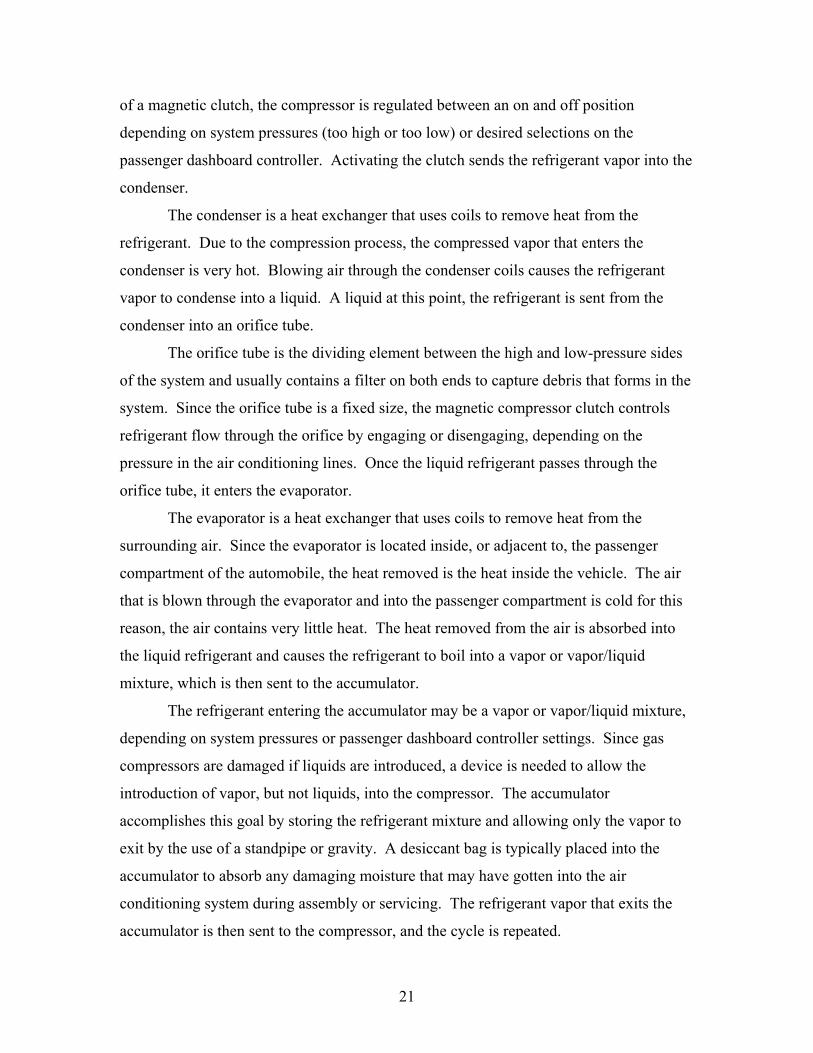
The condenser of an automotive air conditioner was located in the front-end

assembly of a vehicle, right behind the grill. This laboratory test rig front-end assembly,

which consisted of the condenser, radiator, and a window fan, is shown in Figure 4-4. To

simulate an actual automobile, a radiator was placed directly in front of the condenser

and was originally designed to have hot water piped into it resulting in extra heat that

would have to be dissipated by the window fan. Tests could not be performed when the

radiator was used in this capacity because the fan could not provide adequate heat

transfer. As a result, the radiator was left in the assembly, but not used as an extra source

of heat. A 21-inch window fan was placed in front of the assembly and provided airflow

through the radiator and then across the condenser resulting in an adequate and necessary

heat transfer. An oven thermometer placed in the air-flow path behind the condenser

allowed for the measurement of running system condenser temperatures during testing.

Figure 4-4: Condenser, radiator, and fan

25

An actual under-the-dashboard duct system, referred to as the plenum chamber,

was used in the bench test setup as shown in Figure 4-5. Inside, the plenum chamber

contained the integral A/C components (expansion valve and evaporator), and the

auxiliary components that made up the rest of an automobile’s environmental system

(heater coil, blend door, and blower). The hot water tap in the lab allowed the use of the

heater coil to obtain the warm setting on the dashboard controller. The blend door in the

plenum chamber was used to control the mixture of warm and cold air introduced into the

interior of the automobile. A multiple speed blower provided the heat transfer to the air

that would allow the occupants of a vehicle to feel the hot and cold temperature that

results from the heater coil and evaporator, respectively. A 12-volt auto battery provided

the power for the blower in the plenum chamber, the blend door operation, and the

compressor’s magnetic clutch (as mentioned previously). This battery was connected to

a battery charger to prevent battery failure and keep a constant blower speed throughout

the tests performed.

Figure 4-5: Dashboard unit, controller, and ductwork

26

To obtain a temperature-controlled airflow, metal piping was placed on top of the

plenum chamber and designed to mix the cold air from the evaporator with the warm air

from the heater coil upon exiting the plenum chamber. The mixture was then directed

into the intake vent, resulting in a temperature controlled airflow. Preventing the

evaporator from freezing up by allowing more heat transfer to take place is another

benefit from the piping configuration. A thermometer was also placed in the piping for

measuring the resulting air conditioned temperature.

Controlling the blend door and blower speed in the plenum chamber required the

use of a dashboard controller, as shown in Figure 4-6. The dials control the blower

speed, the temperature (blend door control), and the position of the inner workings of the

plenum chamber vents. Unless stated otherwise, tests were performed with the blower

speed on full, the temperature in the middle, and the vent position on defrost as shown in

the figure. The defrost setting engages the compressor and allows the air to run through

the metal piping on the plenum chamber.

Figure 4-6: Dashboard controller

As mentioned in Chapter 1, the accumulator bottle was the point at which the

natural frequency measurements were made. The accumulator bottle of the bench test

setup, which can be seen in Figure 4-7, was held in place two ways—through the inlet

line and the surrounding clamp. The inlet line into the bottle was attached to the line

exiting the plenum chamber, preventing longitudinal movement, and the clamp

encompassing the bottle prevented excessive translational movement.

27

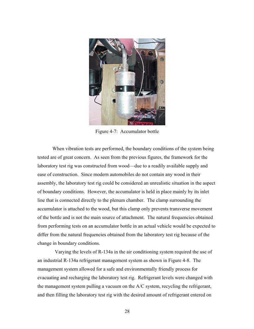
Figure 4-7: Accumulator bottle

When vibration tests are performed, the boundary conditions of the system being

tested are of great concern. As seen from the previous figures, the framework for the

laboratory test rig was constructed from wood—due to a readily available supply and

ease of construction. Since modern automobiles do not contain any wood in their

assembly, the laboratory test rig could be considered an unrealistic situation in the aspect

of boundary conditions. However, the accumulator is held in place mainly by its inlet

line that is connected directly to the plenum chamber. The clamp surrounding the

accumulator is attached to the wood, but this clamp only prevents transverse movement

of the bottle and is not the main source of attachment. The natural frequencies obtained

from performing tests on an accumulator bottle in an actual vehicle would be expected to

differ from the natural frequencies obtained from the laboratory test rig because of the

change in boundary conditions.

Varying the levels of R-134a in the air conditioning system required the use of

an industrial R-134a refrigerant management system as shown in Figure 4-8. The

management system allowed for a safe and environmentally friendly process for

evacuating and recharging the laboratory test rig. Refrigerant levels were changed with

the management system pulling a vacuum on the A/C system, recycling the refrigerant,

and then filling the laboratory test rig with the desired amount of refrigerant entered on

28

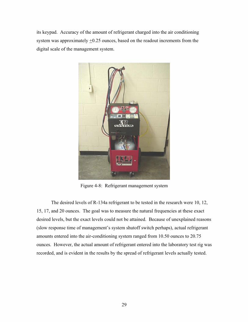
its keypad. Accuracy of the amount of refrigerant charged into the air conditioning

system was approximately +0.25 ounces, based on the readout increments from the

digital scale of the management system.

Figure 4-8: Refrigerant management system

The desired levels of R-134a refrigerant to be tested in the research were 10, 12,

15, 17, and 20 ounces. The goal was to measure the natural frequencies at these exact

desired levels, but the exact levels could not be attained. Because of unexplained reasons

(slow response time of management’s system shutoff switch perhaps), actual refrigerant

amounts entered into the air-conditioning system ranged from 10.50 ounces to 20.75

ounces. However, the actual amount of refrigerant entered into the laboratory test rig was

recorded, and is evident in the results by the spread of refrigerant levels actually tested.

29

4.2 Experimental Setup

As mentioned previously, the accumulator was the chosen location for modal

testing on the laboratory test rig using the roving hammer method. Once the test rig was

built, preliminary modal testing could be performed on the accumulator to find the

optimal locations for the hammer hits as well as accelerometer placements.

To find the optimal location, the hammer and accelerometer were used to obtain

FRFs from different planes on the accumulator. The first objective was to find a plane

where the resulting FRF magnitude would be relatively large and the resulting coherence

would be as close to one as possible. After testing several configurations, vibration along

the x-axis was studied with the test points being located along the z-axis, as shown in

Figure 4-9. This arrangement was chosen for the duration of the laboratory tests due to

the relatively large response. A diagram of the modal analysis testing setup is shown in

Figure 4-9.

Figure 4-9: Modal testing setup

30

It is common in practice to measure FRFs at more than one test point on

structures, due to the possibility of measuring at a node. If the hammer hit occurs at a

node pertaining to a natural frequency of the structure, there will be little or no response

evident in the FRF at that natural frequency. Due to this caveat, the accumulator was

marked and numbered in half-inch intervals starting from the bottom of the cylinder and

moving up. These points were test points of impact for the hammer, and the

accelerometer was placed on the opposite side, as shown in Figure 4-9. The natural

frequencies measured at the different hammer-hit points on the accumulator varied only

in FRF magnitude and coherence. All of the points along the length of the accumulator

were tested and examined to see which points of impact worked best.

Initial testing revealed the first and second natural frequencies to be in the region

of 40 Hz and 1400 Hz respectively. To obtain a desirable coherence in the resulting FRF

at these frequencies, it is necessary that the amount of input power generated by the

hammer be as high as possible at these frequencies. Since the natural frequencies are so

far apart, different hammer tips were used for each natural frequency measurement. The

plastic tip was used for the first natural frequency (0 to 100 Hz range) and a steel tip was

used for the second natural frequency (1 to 1.8 kHz range). The difference between the

autospectrums of the two hammer tips can be seen in Figure 4-10. The steel tip results in

lower power, but extends for a larger useful frequency range. The plastic tip results in

higher power, but extends for a shorter useful frequency range.

Figure 4-10: Autospectrum of different hammer tips

31

Using the impact hammer at the different points along the accumulator also

determines the input frequencies the accelerometer measures. If the input frequency band

dies off at a low frequency, the higher frequencies needing to be analyzed are not picked

up by the accelerometer, resulting in an FRF with low coherence at these higher

frequencies.

It was concluded that measurements would occur at test points 3, 5, and 7 (as

shown in Figure 4-9) for the majority of testing because they are spread over the surface

of the accumulator, and result in a fairly clean response to the input. Test points below

point 3 could not be used due to the difficulty of performing a single (clean) hammer hit

at these points. When using a modal hammer, it is desired to only hit the structure a

single time. Double hammer hits sometimes occur unintentionally due to resonant

systems and cause signal-processing problems that result in inaccurate FRFs.

Because the physical state of the R-134a refrigerant is dependant on pressure, the

laboratory test rig would have to reach steady state conditions before the modal testing of

the accumulator began. Modal tests were performed at different time intervals after the

test rig began operation. From these tests, it was decided that the system would be

allowed to run for ten minutes prior to measuring FRFs from the accumulator for all tests

performed in this research.

4.3 Experimental Procedure

Once the preliminary testing was performed and the location of the hammer hits

and accelerometer placement were found to be optimal, the laboratory rig testing could

begin. The signal analyzer was configured with the proper input and output frequencies

for the hammer and accelerometer, with the number of averages set to three for each

measured FRF. Testing the different refrigerant levels in the laboratory test rig required a

procedure that was repeated for each test.

The accelerometer was attached to the accumulator using wax. The accumulator

had to be dry to use this method of attachment, but once attached, it remained in place

during the testing, even when the surface of the accumulator became cold and wet as a

result from running the air conditioning system.

32

The existing charge in the laboratory test rig would be vacuumed out entirely.

Once empty of refrigerant, the pump on the management system would pull a vacuum on

the system for twenty minutes. The refrigerant management system would then enter an

amount of refrigerant close to the desired amount entered on its keypad. The actual

amount of refrigerant that entered into the test rig was measured using a digital scale with

an accuracy of ± 0.25 ounces. The hoses running from the management system were left

on the laboratory test rig in order to monitor the high and low pressure in the running

system. Using the refrigerant management system required EPA certification, which was

obtained prior to any testing.

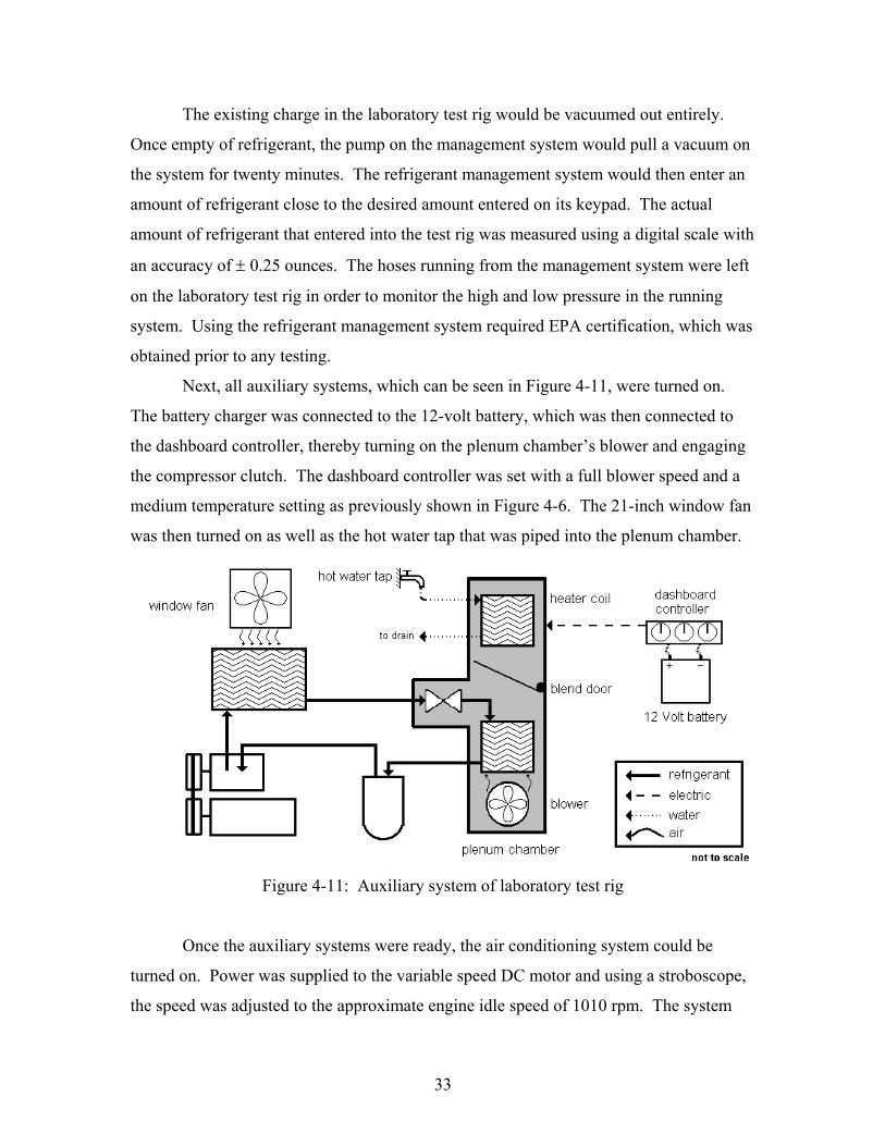
Next, all auxiliary systems, which can be seen in Figure 4-11, were turned on.

The battery charger was connected to the 12-volt battery, which was then connected to

the dashboard controller, thereby turning on the plenum chamber’s blower and engaging

the compressor clutch. The dashboard controller was set with a full blower speed and a

medium temperature setting as previously shown in Figure 4-6. The 21-inch window fan

was then turned on as well as the hot water tap that was piped into the plenum chamber.

Figure 4-11: Auxiliary system of laboratory test rig

Once the auxiliary systems were ready, the air conditioning system could be

turned on. Power was supplied to the variable speed DC motor and using a stroboscope,

the speed was adjusted to the approximate engine idle speed of 1010 rpm. The system

33

would then run for ten minutes to allow for steady state conditions before modal testing

of the accumulator began. Modal testing at the desired points could then occur at the

specified points along the accumulator as shown in Figure 4-12. During the performance

of the modal measurements, the plenum chamber, condenser, and room temperatures

were recorded, as well as the high and low pressures in the air conditioning lines.

Recording these values assisted with the repeatability of the experiments, and the values

of these conditions for the majority of the performed tests (cantilevered and cylindrical

modes for a running, and non-running scenario) are listed in Appendix A. During the

testing phase, two people were always present and knowledgeable of the safety shutoff

switches in the DC motor and of the breaker boxes in the lab. MSDS (material safety

data sheets) were readily available as well.

Figure 4-12: Performance of modal test

Once testing was complete, system shutdown occurred. Power was removed from

the DC motor, the battery was disconnected from the battery charger and dashboard

controller, the 21-inch window fan was off, and the hot water tap valve was closed. Then

the refrigerant would be vacuumed out, which was the longest process of testing. The

low pressures in the system would cause the refrigerant to liquefy, leaving some in the

system after initial vacuuming. To insure all refrigerant was removed from the system,

34

the refrigerant in the system would be allowed to evaporate fully, and then the refrigerant

could be removed. Depending on the amount of R-134a in the system, this would take

anywhere from thirty minutes to an hour. Once the system was empty, the entire

procedure would be repeated for the next desired refrigerant level to be tested.

35

Chapter 5

Frequency Response Analysis

5.1 General Overview

Frequency response functions (FRFs) were obtained at the accumulator bottle for

the various levels of R-134a refrigerant. The resulting FRFs were used to experimentally

find the natural frequencies and confirm the hypothesis that the natural frequencies of the

accumulator bottle are a function of the level of R-134a refrigerant in the system. Two

natural frequencies of the accumulator bottle were examined. The natural frequency in

the region of 45 Hz was identified and was determined to be the cantilever mode of the

accumulator-inlet line assembly. The natural frequency in the region of 1400 Hz was

identified and was determined to be a cylindrical mode of the accumulator. The modal

(vibration) tests were performed with the air conditioning system in operation. In

addition, parameter studies were also performed to examine how the measured natural

frequency would be affected under various conditions. These tests included:

Varying tightness of the accumulator bottle clamp

Alternate accelerometer placement

Varying dashboard controller settings

Transient system measurements

Non-running system measurements

5.2 Mode Shapes of the Accumulator Bottle

The mode shapes of the accumulator bottle were addressed to determine which

natural frequencies were being examined during the modal testing. The mode shape

corresponding to the first studied natural frequency could be plotted directly from the

36

measured FRFs, while the second studied natural frequency mode shape required less

quantitative analysis and more qualitative analysis of the measured FRFs.

If the natural frequencies are well separated, one method used to experimentally

obtain the mode shapes involves placing the accelerometer in one location on the

accumulator, then using the impact hammer to obtain FRFs along many points on the

accumulator. The imaginary value of the FRF at a natural frequency, measured at a

certain point on the accumulator bottle, is the relative displacement at that point. Once

several points along the length of the accumulator bottle were tested, the displacements

were plotted spatially, resulting in the mode shapes.

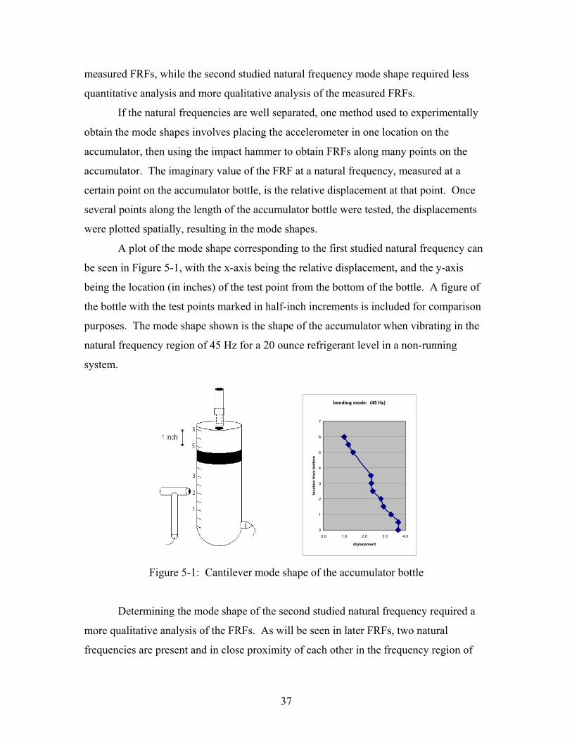
A plot of the mode shape corresponding to the first studied natural frequency can

be seen in Figure 5-1, with the x-axis being the relative displacement, and the y-axis

being the location (in inches) of the test point from the bottom of the bottle. A figure of

the bottle with the test points marked in half-inch increments is included for comparison

purposes. The mode shape shown is the shape of the accumulator when vibrating in the

natural frequency region of 45 Hz for a 20 ounce refrigerant level in a non-running

system.

bending mode: (45 Hz)

0

1

2

3

4

5

6

7

0.0 1.0 2.0 3.0 4.0

diplacement

loca

tion

from

bot

tom

Figure 5-1: Cantilever mode shape of the accumulator bottle

Determining the mode shape of the second studied natural frequency required a

more qualitative analysis of the FRFs. As will be seen in later FRFs, two natural

frequencies are present and in close proximity of each other in the frequency region of

37

1400 Hz, with only the dominant natural frequency’s phase equaling –90 degrees.

Because of the close proximity of the two natural frequencies, the mode shapes could not

be plotted using the previous method. If another natural frequency is in close proximity

to another, they affect each others response, and the mode shapes obtained are not

accurate. Requiring additional impact hits from the hammer, the type of mode of the

accumulator at the dominant natural frequency was discovered and the details of the

process can be found in Appendix B.

From the analysis of the FRFs, the experimental mode shapes of the accumulator

bottle were established. In the low frequency region of 45 Hz, the accumulator bottle

vibrates as a mass at the end of the inlet line that acts as a cantilevered beam. In the

higher frequency region of 1400 Hz, the mode shape of the accumulator is a radial-axial

mode of a cylinder. The mode shapes of the accumulator bottle as described are

illustrated in Figure 5-2, with dashed lines representing the accumulator at rest. The

illustration for the cylindrical mode is only one possibility of the actual mode of the

cylinder at the tested natural frequency (actual mode may be of a higher order).

Figure 5-2: Studied modes of accumulator bottle: (a) cantilever (b) cylindrical

The natural frequencies of the accumulator bottle were analytically estimated and

compared with the experimentally obtained natural frequencies and mode shapes. From

the calculations, it was inferred that the mode shapes determined from experimental

analysis are accurate. Details of the calculated natural frequencies and corresponding

theoretical mode shapes can be seen in Appendix C.

38

5.3 Cantilever Natural Frequency

The natural frequency of the accumulator bottle in the 45 Hz frequency region

was identified as the cantilevered natural frequency. Because the examined frequencies

were low and the input power was desired to be as large as possible, the plastic

(polycarbonate) tip was used on the impact hammer to obtain the FRFs for this natural

frequency. The air conditioning system was running as the data was collected at test

points 3, 5, and 7 on the accumulator bottle. Resulting FRFs corresponding to varying R-

134a refrigerant levels for a particular series of tests are shown in Figure 5-1. Natural

frequencies were identified by determining the frequency at which the phase crosses +90

degrees (the dashed line). The FRFs illustrate the inverse relationship between natural

frequency and refrigerant level—as the R-134a level increases, the measured natural

frequency decreases.

Figure 5-3: FRF of cantilever natural frequencies for various R-134a levels

Two series of tests were performed in cantilever natural frequency region for the

various levels of R-134a, and the resulting experimental natural frequencies measured are

39

shown graphically in Figure 5-4, and the numerical values are presented in Table 5-1.

The test numbers listed correspond to the date of testing and the point of hammer impact

(for example, testing that occurred on August 13 and impacted at point 3 on the

accumulator bottle is designated test 713-3).

Measurement Data Spread

384042444648505254

8.00 10.00 12.00 14.00 16.00 18.00 20.00 22.00

R-134a charge

natu

ral f

requ

ency

(Hz)

831-3831-5831-71016-31016-51016-7

Figure 5-4: Cantilever natural frequency vs. R-134a level in running system

Table 5-1: Natural frequencies (Hz) for varying levels of R-134a (cantilever mode)

R-134a Level (oz) Test 20.25 20.00 17.00 15.50 12.75 11.00 10.50 831-3 40 N/A 43 45 50 52 N/A 831-5 40 N/A 43 46 51 52 N/A 831-7 40 N/A 43 45 49 50 N/A 1016-3 N/A 43 N/A 48 N/A N/A 49 1016-5 N/A 43 N/A 48 N/A N/A 49 1016-7 N/A 43 N/A 48 N/A N/A 48

The results from the two series of running laboratory air conditioning system tests

indicate an approximate R-134a measurement accuracy of ±2.5 ounces as determined

from the cantilever natural frequency. As shown in Figure 5-4 and Table 5-1, the

frequency difference between the lowest and highest level of R-134a is at most 12 Hz.

40

The natural frequencies for the lower refrigerant levels (the 15, 12 and 10 ounce charges)

were also very close together, with a one or two Hertz difference. The narrow frequency

bandwidth may cause difficulties in distinguishing one refrigerant level from another

when trying to determine the refrigerant charge from experimentally obtained natural

frequencies. Another concern that existed at this low frequency region was how the

boundary conditions of the accumulator would affect the measured natural frequencies.

This concern existed for the cylindrical natural frequency as well, but due to time

constraints, boundary condition tests at the cylindrical natural frequency were not

performed.

5.3.1 Effects of Accumulator Clamp Tightness

When calculating or measuring the natural frequencies of vibrating systems, the

boundary conditions of the system have a direct effect on the results. As stated earlier,

the accumulator bottle was connected to the vehicle through the inlet A/C line and the

surrounding clamp. This clamp was held together and connected to the vehicle’s firewall

by a bolt. During the assembly of the air conditioning system, the tightness of the clamp

bolt could vary from one vehicle to the next. Changing the tightness of the clamp-bolt

(the boundary condition) could possibly result in different measured natural frequencies

for the same level of refrigerant in the same type of vehicle.

The clamp-bolt tightness in the laboratory test rig was varied to examine the

effect on the cantilever natural frequency. FRFs were measured in a running system at

test points 3, 5, and 7, with a 20 ounce R-134a charge. The results of this parameter test

can be seen in Figure 5-5, with each FRF indicating a different clamp-bolt tightness.

Measured with a torque wrench, the tested bolt tightness was 75 in-lb, 50 in-lb, and

25 in-lb. The 25 in-lb torque was considered to be the nominal “hand-tightened”

scenario. The data denoted as ½, 1, and 1½ turns are the number of turns of the bolt after

torque could no longer be measured or simply a measure of “looseness” of the bolt.

41

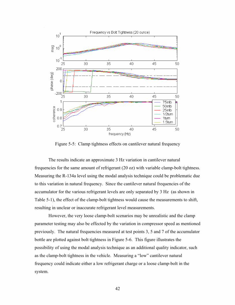
Figure 5-5: Clamp tightness effects on cantilever natural frequency

The results indicate an approximate 3 Hz variation in cantilever natural

frequencies for the same amount of refrigerant (20 oz) with variable clamp-bolt tightness.

Measuring the R-134a level using the modal analysis technique could be problematic due

to this variation in natural frequency. Since the cantilever natural frequencies of the

accumulator for the various refrigerant levels are only separated by 3 Hz (as shown in

Table 5-1), the effect of the clamp-bolt tightness would cause the measurements to shift,

resulting in unclear or inaccurate refrigerant level measurements.

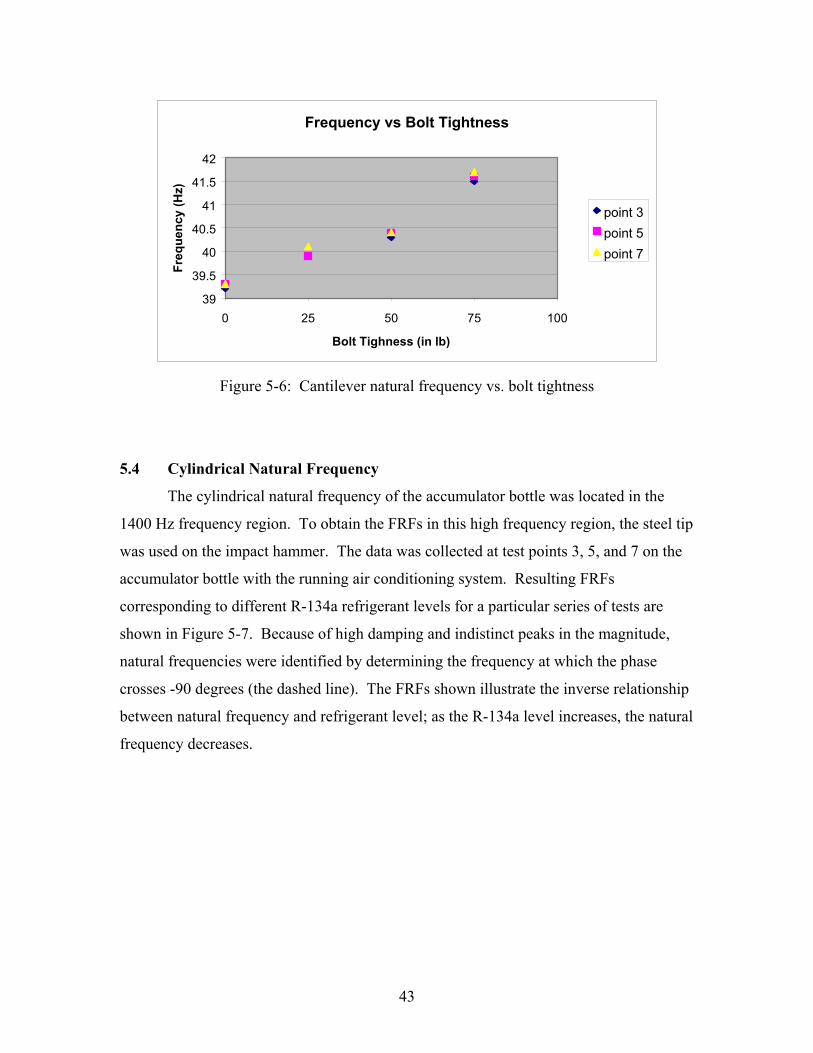
However, the very loose clamp-bolt scenarios may be unrealistic and the clamp

parameter testing may also be effected by the variation in compressor speed as mentioned

previously. The natural frequencies measured at test points 3, 5 and 7 of the accumulator

bottle are plotted against bolt tightness in Figure 5-6. This figure illustrates the

possibility of using the modal analysis technique as an additional quality indicator, such

as the clamp-bolt tightness in the vehicle. Measuring a “low” cantilever natural

frequency could indicate either a low refrigerant charge or a loose clamp-bolt in the

system.

42

Frequency vs Bolt Tightness

39

39.5

40

40.5

41

41.5

42

0 25 50 75 100

Bolt Tighness (in lb)

Freq

uenc

y (H

z)

point 3point 5point 7

Figure 5-6: Cantilever natural frequency vs. bolt tightness

5.4 Cylindrical Natural Frequency

The cylindrical natural frequency of the accumulator bottle was located in the

1400 Hz frequency region. To obtain the FRFs in this high frequency region, the steel tip

was used on the impact hammer. The data was collected at test points 3, 5, and 7 on the

accumulator bottle with the running air conditioning system. Resulting FRFs

corresponding to different R-134a refrigerant levels for a particular series of tests are

shown in Figure 5-7. Because of high damping and indistinct peaks in the magnitude,

natural frequencies were identified by determining the frequency at which the phase

crosses -90 degrees (the dashed line). The FRFs shown illustrate the inverse relationship

between natural frequency and refrigerant level; as the R-134a level increases, the natural

frequency decreases.

43

Figure 5-7: FRF plot of cylindrical natural frequencies for various R-134a levels

A definite phase of –90 degrees was evident for the higher levels of R-134a, but

for lower levels, the phase did not cross the −90 degree line. The most likely reason for

this can be attributed to another natural frequency in close proximity to the one being

measured. If another natural frequency is in close proximity to another, they begin to

affect each others response. The effected response is most noticeable in the phase plot,

where the phase at one natural frequency prevents another natural frequency’s phase from

equaling –90 degrees.

The FRFs at the cylindrical natural frequency also show the coherence beginning

to drop below 0.98 at frequencies around 1440 Hz and above. Lower coherence can be

attributed to the input force, provided by the impact hammer, dropping below optimum

excitation levels. In practice, the frequency limit for input excitations is the frequency

where the excitation’s power level drops 10 or 20 dB below its maximum value.

Examining the autospectrum of the input gives an indication of the amount of input force,

or power used to excite the system. For the cylindrical natural frequency tests, the input

autospectrum provided by the impact hammer with the steel tip can be seen in Figure 5-8.

44

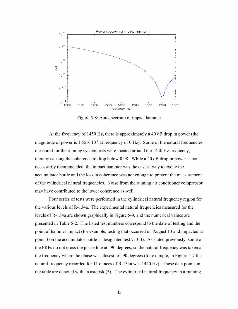
Figure 5-8: Autospectrum of impact hammer

At the frequency of 1450 Hz, there is approximately a 40 dB drop in power (the

magnitude of power is 1.55 × 10-6 at frequency of 0 Hz). Some of the natural frequencies

measured for the running system tests were located around the 1440 Hz frequency,

thereby causing the coherence to drop below 0.98. While a 40 dB drop in power is not

necessarily recommended, the impact hammer was the easiest way to excite the

accumulator bottle and the loss in coherence was not enough to prevent the measurement

of the cylindrical natural frequencies. Noise from the running air conditioner compressor

may have contributed to the lower coherence as well.

Four series of tests were performed in the cylindrical natural frequency region for

the various levels of R-134a. The experimental natural frequencies measured for the

levels of R-134a are shown graphically in Figure 5-9, and the numerical values are

presented in Table 5-2. The listed test numbers correspond to the date of testing and the

point of hammer impact (for example, testing that occurred on August 13 and impacted at

point 3 on the accumulator bottle is designated test 713-3). As stated previously, some of

the FRFs do not cross the phase line at –90 degrees, so the natural frequency was taken at

the frequency where the phase was closest to –90 degrees (for example, in Figure 5-7 the

natural frequency recorded for 11 ounces of R-134a was 1440 Hz). These data points in

the table are denoted with an asterisk (*). The cylindrical natural frequency in a running

45

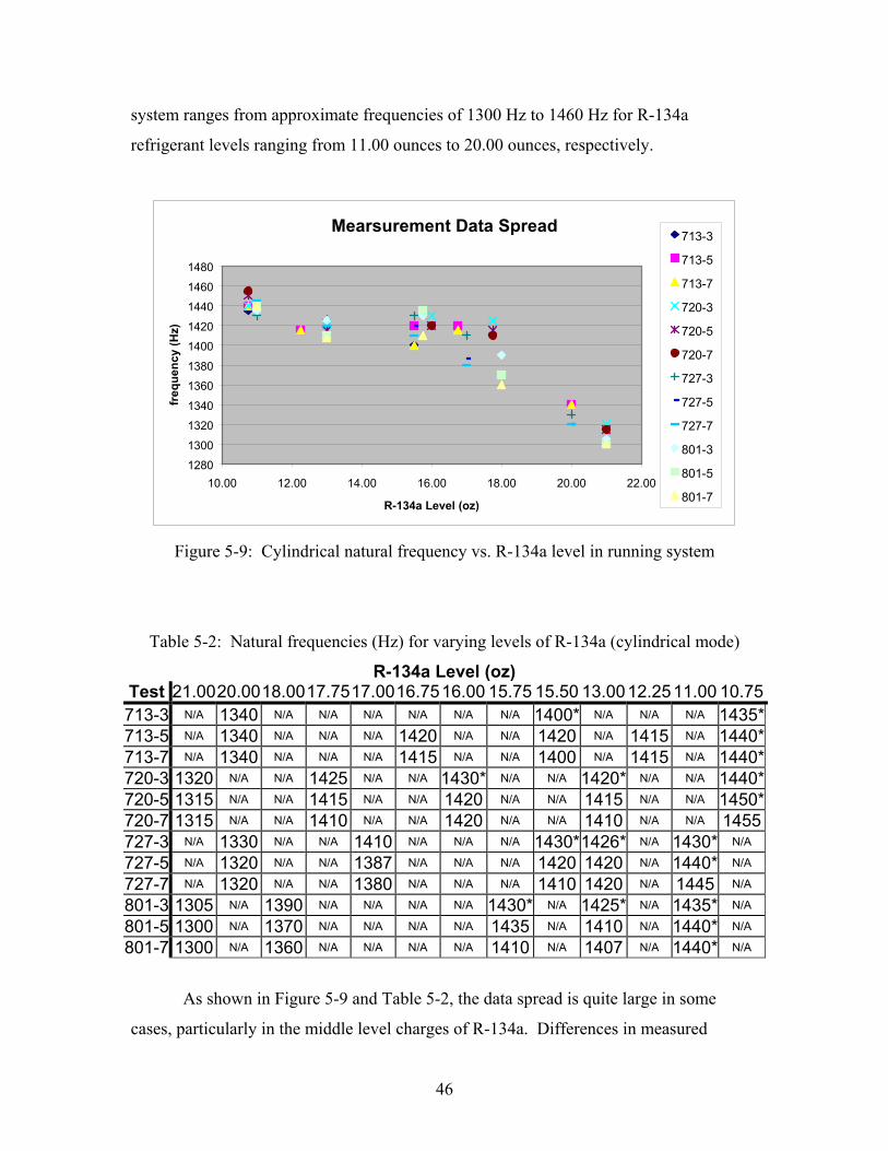
system ranges from approximate frequencies of 1300 Hz to 1460 Hz for R-134a

refrigerant levels ranging from 11.00 ounces to 20.00 ounces, respectively.

Mearsurement Data Spread

12801300132013401360138014001420144014601480

10.00 12.00 14.00 16.00 18.00 20.00 22.00

R-134a Level (oz)

freq

uenc

y (H

z)

713-3

713-5

713-7

720-3

720-5

720-7

727-3

727-5

727-7

801-3

801-5

801-7

Figure 5-9: Cylindrical natural frequency vs. R-134a level in running system

Table 5-2: Natural frequencies (Hz) for varying levels of R-134a (cylindrical mode)

R-134a Level (oz) Test 21.00 20.00 18.00 17.75 17.0016.7516.00 15.75 15.50 13.00 12.25 11.00 10.75713-3 N/A 1340 N/A N/A N/A N/A N/A N/A 1400* N/A N/A N/A 1435*713-5 N/A 1340 N/A N/A N/A 1420 N/A N/A 1420 N/A 1415 N/A 1440*713-7 N/A 1340 N/A N/A N/A 1415 N/A N/A 1400 N/A 1415 N/A 1440*720-3 1320 N/A N/A 1425 N/A N/A 1430* N/A N/A 1420* N/A N/A 1440*720-5 1315 N/A N/A 1415 N/A N/A 1420 N/A N/A 1415 N/A N/A 1450*720-7 1315 N/A N/A 1410 N/A N/A 1420 N/A N/A 1410 N/A N/A 1455727-3 N/A 1330 N/A N/A 1410 N/A N/A N/A 1430*1426* N/A 1430* N/A 727-5 N/A 1320 N/A N/A 1387 N/A N/A N/A 1420 1420 N/A 1440* N/A 727-7 N/A 1320 N/A N/A 1380 N/A N/A N/A 1410 1420 N/A 1445 N/A 801-3 1305 N/A 1390 N/A N/A N/A N/A 1430* N/A 1425* N/A 1435* N/A 801-5 1300 N/A 1370 N/A N/A N/A N/A 1435 N/A 1410 N/A 1440* N/A 801-7 1300 N/A 1360 N/A N/A N/A N/A 1410 N/A 1407 N/A 1440* N/A

As shown in Figure 5-9 and Table 5-2, the data spread is quite large in some

cases, particularly in the middle level charges of R-134a. Differences in measured

46

natural frequencies range from 50 to 10 Hz for a given level of R-134a. These

discrepancies among data points may be due to the problem of compressor speed

variations in the laboratory system. Changing the compressor speed effects the pressure

in the system, which then causes the composition of the refrigerant in the accumulator

bottle to change, resulting in an unsteady system.

The results from the running laboratory air conditioning system indicate an

approximate R-134a measurement accuracy of ±3 ounces as determined from the

cylindrical natural frequency. Because the cylindrical natural frequency has a larger

difference in frequencies between refrigerant levels, most laboratory tests were

performed examining the cylindrical natural frequency response.

5.4.1 Effect of Accelerometer Placement

Previous testing was performed with the accelerometer placed across from test

point 1 as shown in the experimental setup section (for reference, see Figure 3-9). The

accelerometer was moved from its original position to a new position located across from

test point 8. Being the approximate center of the bottle, test point 8 is the point of

maximum deflection of the bottle at the examined cylindrical natural frequency as

previously shown in the plots of the measured mode shapes of Figure 5-1. Because it is

the point of maximum deflection, the output of the accelerometer should be larger in

magnitude if the accelerometer were placed back in the original position.

Modal analysis was performed with the new placement of the accelerometer for

R-134a refrigerant levels of 10.50, 15.50, and 20.00 ounces. A plot with the comparison

between FRFs for the two different accelerometer placements for a 15 ounce R-134a

charge can be seen in Figure 5-10. The placement of the accelerometer at point 8 results

in a larger magnitude, an approximate increase of 20 in magnitude, than the

original placement due to the larger response of the accelerometer at the center of the

accumulator bottle. Although the magnitudes of the measured FRFs are different, the

relative shape of both is the same.

/Nsm 2−⋅

47

Figure 5-10: Location effect of accelerometer on cylindrical mode

The FRFs for varying R-134a levels with the new placement of the

accelerometer can be seen in Figure 5-11. Placing the accelerometer at point 8 resulted in

a more evident appearance of the close natural frequency to the one being measured. The

close natural frequency causes the phases of the lower refrigerant levels to cross the –90

degree phase line unlike previous tests where the lower refrigerant level phases did not

cross this line at all. This early crossing of the phase line could cause problems if the

refrigerant levels were measured without visually examining the resulting FRFs. If

analyzing the results of the FRF numerically, the distinction between R-134a levels

would be very difficult to determine.

48

Figure 5-11: FRF of new accelerometer placement for various R-134a levels

The placement of the accelerometer is important in determining refrigerant levels

from measuring the natural frequency of the accumulator bottle. As shown, some

locations actually bring out natural frequencies that are as evident at other locations. If

this method were to be used in the field, a point on the accumulator bottle would have to

be specified to avoid confusion in analyzing the results.

5.4.2 Effect of Dashboard Controller Setting

As explained in the experimental setup section, the modal analysis tests were

performed on the accumulator bottle with the dashboard controller set to the

configuration shown in Figure 4-6. To test how these dashboard control settings effect

the measurements of the natural frequencies, tests were performed with varied

temperature control settings. It was originally desired to test the effect of blower speed as

well. However, attempting to run the air conditioning system with blower speed settings

other than full resulted in high pressures that would disengage the compressor clutch,

49

resulting in an unstable system. Leaving the fan speed on high, the temperature control

could be moved to full cold, half cold, and middle temperature as seen in Figure 5-12.

Once the temperature control was placed on the desired setting, the system was allowed

to run for five minutes to achieve a steady state composition of R-134a in the

accumulator. Modal tests were then performed with the system at these settings and with

R-134a levels of 10.50, 15.50, and 20.00 ounces.

Figure 5-12: Dashboard controller settings tested

The resulting FRFs comparing the effect of the different thermostat settings on the

cylindrical natural frequency are shown in Figures 5-13, Figure 5-14, and Figure 5-14 for

the tested levels of R-134a. The labels mid, half, and full in the figures denote the

middle, half cold, and full cold temperature settings shown in Figure 5-12. The

temperature in the plenum chamber was measured during the testing process as well.

Ranging from 49 degrees Fahrenheit to 79 degrees Fahrenheit, these temperatures are

listed in Table 5-3.

50

Figure 5-13: FRF of various temperature control settings (10.50 ounces)

Figure 5-14: FRF of various temperature control settings (15.50 ounces)

51

Figure 5-15: FRF of various temperature control settings (20.00 ounces)

Table 5-3: Temperatures for varying thermostat settings

R-134a Level Mid Setting ½ Cold Setting Full Cold Setting

10 ounce 79 F 83 F 70F

15 ounce 64 F 54 F 44 F

20 ounce 77 F 54 F 48 F

The measured cylindrical natural frequencies of the accumulator bottle for each

dashboard temperature setting tested are listed in Table 5-4. From the table, it can be

seen that the differences in cylindrical natural frequencies are: 35 Hz for a 10.50 ounce

charge, 27 Hz for a 15.50 ounce charge, and 100 Hz for a 20.00 ounce R-134a charge.

These differences could prevent a high level of accuracy in the modal testing of the

accumulator bottle. If the modal analysis method were to be used in the field, a

52

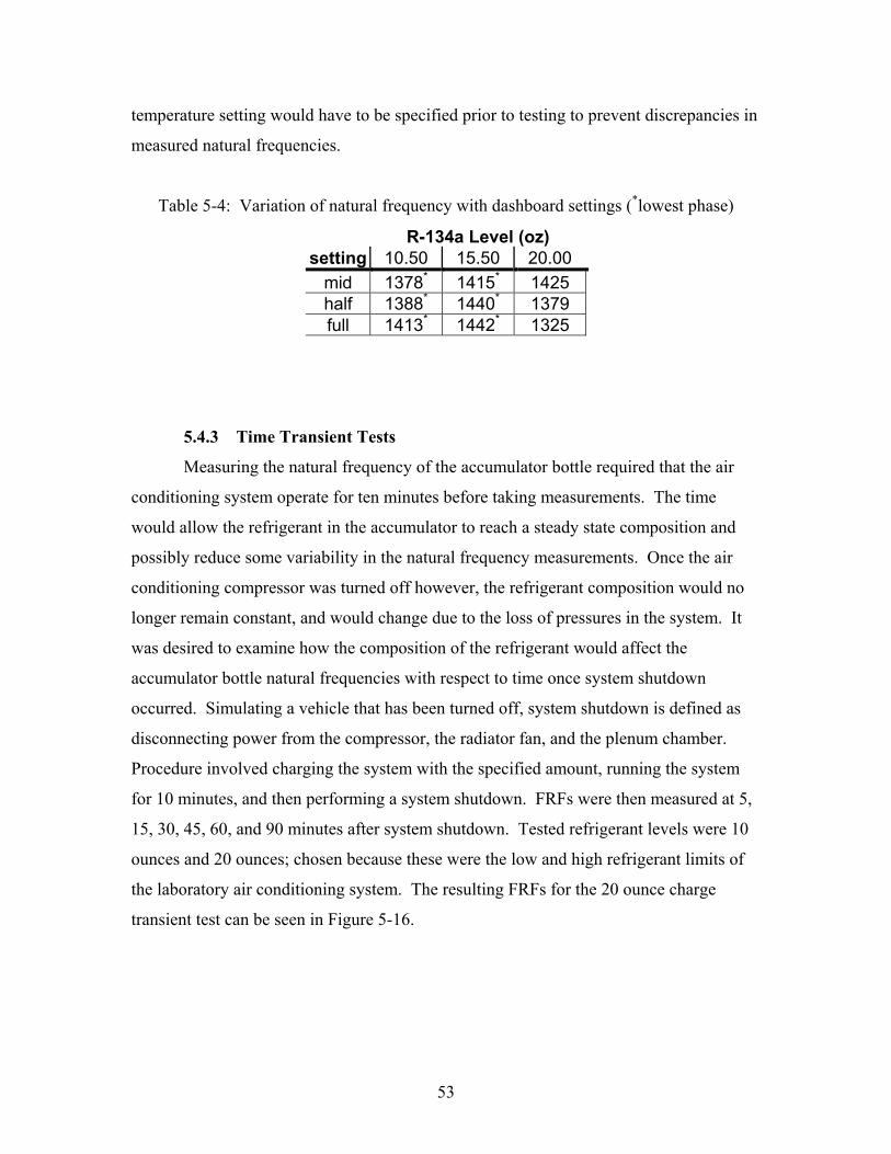
temperature setting would have to be specified prior to testing to prevent discrepancies in

measured natural frequencies.

Table 5-4: Variation of natural frequency with dashboard settings (*lowest phase)

R-134a Level (oz) setting 10.50 15.50 20.00

mid 1378* 1415* 1425

half 1388* 1440* 1379 full 1413* 1442* 1325

5.4.3 Time Transient Tests

Measuring the natural frequency of the accumulator bottle required that the air

conditioning system operate for ten minutes before taking measurements. The time

would allow the refrigerant in the accumulator to reach a steady state composition and

possibly reduce some variability in the natural frequency measurements. Once the air

conditioning compressor was turned off however, the refrigerant composition would no

longer remain constant, and would change due to the loss of pressures in the system. It

was desired to examine how the composition of the refrigerant would affect the

accumulator bottle natural frequencies with respect to time once system shutdown

occurred. Simulating a vehicle that has been turned off, system shutdown is defined as

disconnecting power from the compressor, the radiator fan, and the plenum chamber.

Procedure involved charging the system with the specified amount, running the system

for 10 minutes, and then performing a system shutdown. FRFs were then measured at 5,

15, 30, 45, 60, and 90 minutes after system shutdown. Tested refrigerant levels were 10

ounces and 20 ounces; chosen because these were the low and high refrigerant limits of

the laboratory air conditioning system. The resulting FRFs for the 20 ounce charge

transient test can be seen in Figure 5-16.

53

Figure 5-16: Transient test of 20.00 ounce R-134a charge

The transient test results illustrate some important details in the measurement of

the accumulator natural frequencies. The most noticeable characteristic of the transient

test FRFs is the definite appearance of another close natural frequency, as indicated by

the two peaks in the magnitude plot. This other natural frequency was not very evident in

the running system FRFs. For the research presented, the second peak shown in Figure

5-16 was used to record the natural frequency, since the phase at this peak does cross the

–90 degree phase line. The mode shape obtained from the second peak shown was the

previously discussed “cylindrical mode” of the accumulator bottle.

The natural frequency range for a system that has been shutdown is lower than the

natural frequencies of a running system as well. Here, they are in the frequency range of

1250 Hz compared to the frequencies of 1450 Hz for a running system. The coherence is

also improved, due to the lower frequency range and less noise in the system because the

compressor is no longer running.

The FRF for a transient test with a 10.25 ounce R-134a charge can be seen in

Figure 5-17. Comparing the results of the 10 ounce and 20 ounce tests indicate that the

larger the refrigerant level, the more time it takes for the refrigerant to reach steady state.

54

Figure 5-17: Transient test of 10.25 ounce R-134a charge

Test results indicated a difference between natural frequencies from five minutes

to ninety minutes after system shutoff. The differences in natural frequencies between a

measurement at 5 minutes and a measurement at 90 minutes is 5 Hz for a 10.50 ounce R-

134a charge, and 19 Hz for a 20.00 ounce R-134a charge. Shutting the system off results

in a change of the R-134a’s physical state, resulting in an effective mass change in the

accumulator.

It must be noted that the results of this test are may be reliant on the ambient

temperature of the laboratory. Since the physical state of R-134a is dependant on

temperature as well as pressure, a different ambient temperature than present in the

laboratory (approximately 75° F) could cause the equilibrium time of the refrigerant to

differ, and the natural frequencies would shift. This is merely a caveat that could affect

the accuracy of the measurements if the modal analysis method was to be used in the

field.

55

5.4.4 Non-running System Tests

Natural frequencies of the accumulator bottle for varying amounts of R-134a were

measured in a non-running air condition system scenario. Procedure for this series of

tests involved loading the desired amount of refrigerant into the air conditioning system,

running the system for ten minutes, and then performing a system shutdown. Using the

results from the transient test data, it was determined that the natural frequency

measurements would occur thirty minutes after system shutdown. For a 20 ounce charge,

the difference in natural frequencies between waiting ninety minutes and thirty minutes

before taking measurements was only 5 Hz. This was considered reasonable, since the

difference was small and data needed to be obtained in a realistic amount of time.

Resulting FRFs corresponding to different R-134a refrigerant levels for a particular series

of non-running system tests are shown in Figure 5-18.

Figure 5-18: FRF plot of cylindrical natural frequencies of various R-134a levels

The FRFs obtained from a non-running system illustrate the same results that are

present in the transient test FRFs. A double peak that was not very evident in the running

system tests appears in the non-running system magnitude plot, which indicates there is a

56

natural frequency close to the one that is being measured. For the research presented, the

second peak shown in Figure 5-18 was used to record the natural frequency, since the

phase crosses the –90 degree phase line at this peak. The mode shape obtained from the

second peak shown was the previously discussed cylindrical mode of the accumulator

bottle

The natural frequencies obtained from a non-running system are lower than the

natural frequencies of a running system as expected due to the settling out of the

refrigerant in the accumulator bottle. Here, they are in the range of 1250 Hz compared to

the frequencies of 1450 Hz for a running system. The coherence is also improved as well

due to the lower frequency range and less noise in the system because the compressor is

no longer running.

Four series of tests were performed in the non-running system scenario for

various levels of R-134a. The experimental natural frequencies measured for the levels

of R-134a are shown graphically in Figure 5-19, and the numerical values are presented

in Table 5-5. The listed test numbers correspond to the date of testing and the point of

hammer impact (for example, testing that occurred on August 13 and impacted at point 3

on the accumulator bottle is designated test 713-3). The refrigerant levels tested also

indicate the tendency of the refrigerant management system to overshoot the original

desired refrigerant levels. The cylindrical natural frequency in a non-running system

ranges from approximate frequencies of 1230 Hz to 1380 Hz for R-134a refrigerant

levels ranging from 10.00 ounces to 21.00 ounces.

57

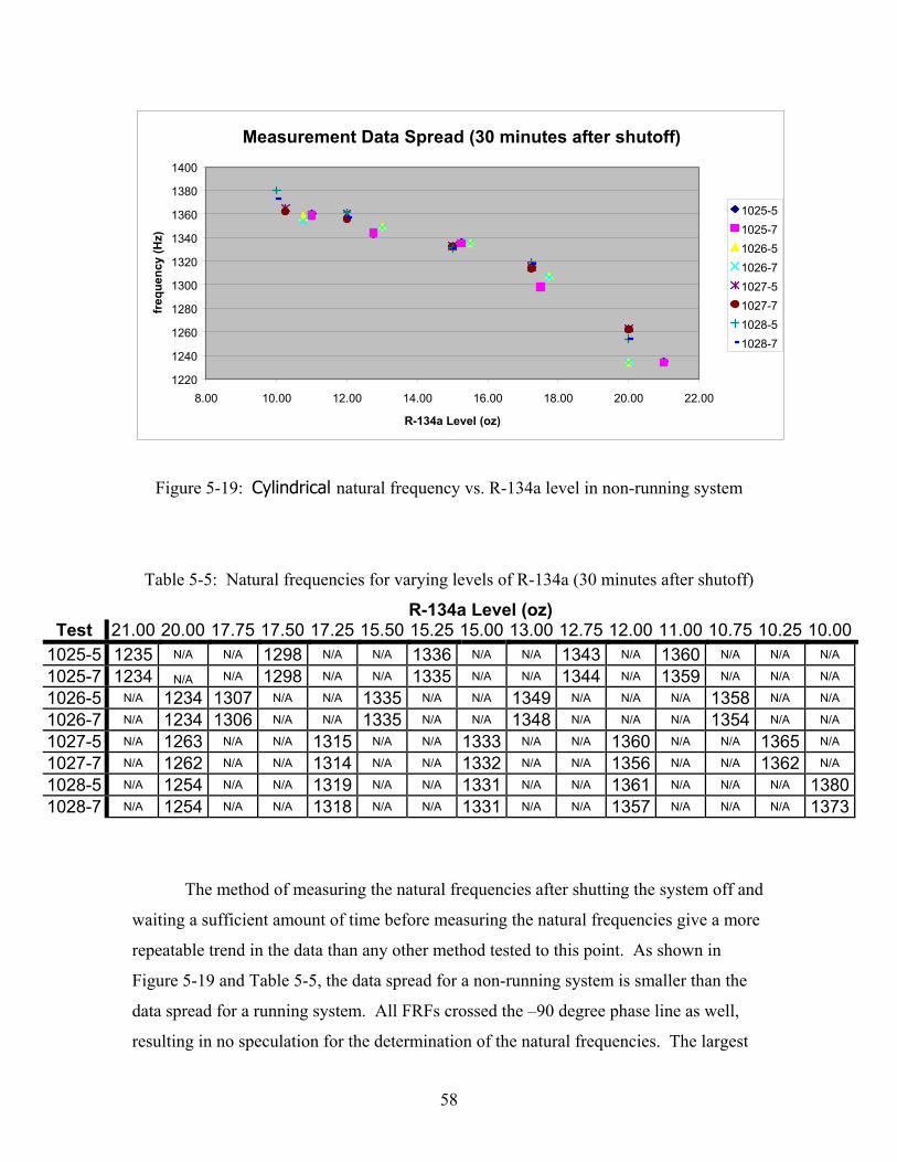
Measurement Data Spread (30 minutes after shutoff)

1220

1240

1260

1280

1300

1320

1340

1360

1380

1400

8.00 10.00 12.00 14.00 16.00 18.00 20.00 22.00

R-134a Level (oz)

freq

uenc

y (H

z)

1025-51025-71026-51026-71027-51027-71028-51028-7

Figure 5-19: Cylindrical natural frequency vs. R-134a level in non-running system

Table 5-5: Natural frequencies for varying levels of R-134a (30 minutes after shutoff)

R-134a Level (oz) Test 21.00 20.00 17.75 17.50 17.25 15.50 15.25 15.00 13.00 12.75 12.00 11.00 10.75 10.25 10.00

1025-5 1235 N/A N/A 1298 N/A N/A 1336 N/A N/A 1343 N/A 1360 N/A N/A N/A

1025-7 1234 N/A N/A 1298 N/A N/A 1335 N/A N/A 1344 N/A 1359 N/A N/A N/A

1026-5 N/A 1234 1307 N/A N/A 1335 N/A N/A 1349 N/A N/A N/A 1358 N/A N/A

1026-7 N/A 1234 1306 N/A N/A 1335 N/A N/A 1348 N/A N/A N/A 1354 N/A N/A

1027-5 N/A 1263 N/A N/A 1315 N/A N/A 1333 N/A N/A 1360 N/A N/A 1365 N/A

1027-7 N/A 1262 N/A N/A 1314 N/A N/A 1332 N/A N/A 1356 N/A N/A 1362 N/A

1028-5 N/A 1254 N/A N/A 1319 N/A N/A 1331 N/A N/A 1361 N/A N/A N/A 13801028-7 N/A 1254 N/A N/A 1318 N/A N/A 1331 N/A N/A 1357 N/A N/A N/A 1373

The method of measuring the natural frequencies after shutting the system off and

waiting a sufficient amount of time before measuring the natural frequencies give a more

repeatable trend in the data than any other method tested to this point. As shown in

Figure 5-19 and Table 5-5, the data spread for a non-running system is smaller than the

data spread for a running system. All FRFs crossed the –90 degree phase line as well,

resulting in no speculation for the determination of the natural frequencies. The largest

58

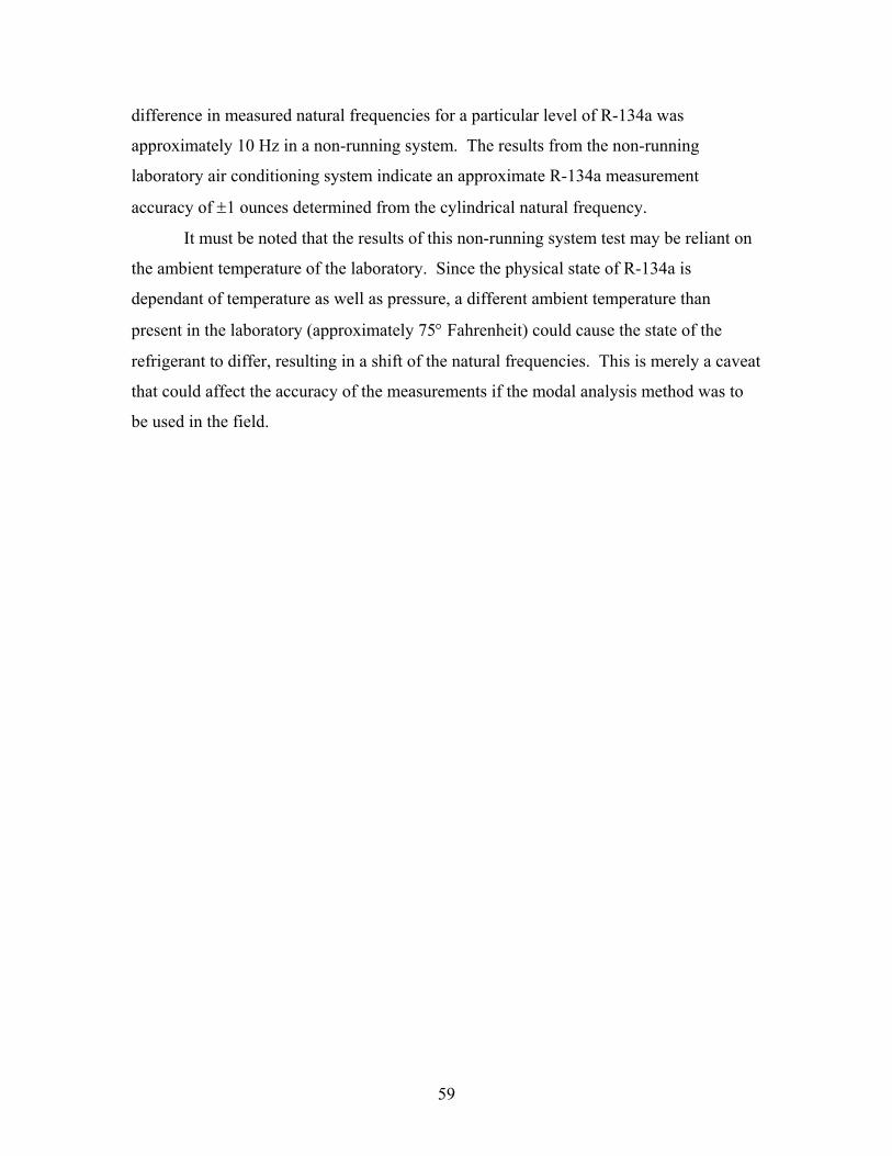
difference in measured natural frequencies for a particular level of R-134a was

approximately 10 Hz in a non-running system. The results from the non-running

laboratory air conditioning system indicate an approximate R-134a measurement

accuracy of ±1 ounces determined from the cylindrical natural frequency.

It must be noted that the results of this non-running system test may be reliant on

the ambient temperature of the laboratory. Since the physical state of R-134a is

dependant of temperature as well as pressure, a different ambient temperature than

present in the laboratory (approximately 75° Fahrenheit) could cause the state of the

refrigerant to differ, resulting in a shift of the natural frequencies. This is merely a caveat

that could affect the accuracy of the measurements if the modal analysis method was to

be used in the field.

59

Chapter 6

Conclusions and Future Work

6.1 Overview of work completed

The purpose of this research was to investigate a new method for measuring

refrigerant R-134a level in automobile air conditioning systems. The desire to improve

quality control in assembly lines and detect leaks in automobile air conditioning systems

provided the motivation for the research. Current methods used to measure refrigerant

levels in automobile air conditioners are not very accurate or efficient.

Experimental modal analysis was the new method applied in the research for

measuring R-134a refrigerant level. Modal analysis is used in industry to find natural

frequencies of systems and has even been implemented in research to measure liquid

levels in various containers. For the research presented, the modal analysis technique

was used to find and locate the natural frequency of the accumulator bottle of the

automotive air conditioner system. Since natural frequencies are a function of mass, the

natural frequency of the accumulator becomes a function of the amount (mass) of the R-

134a refrigerant in the system. An impact hammer, an accelerometer, and a signal

analyzer were used to obtain the frequency response functions (FRFs). The FRFs were

analyzed, resulting in the determination of and the natural frequencies of the accumulator

bottle.

A laboratory test rig was constructed to test the studied modal analysis method.

Consisting of automotive air conditioning system components, the test rig was operated

at actual engine idle speeds and had full use of the dashboard controller (fan and

temperature settings). During operation of the test rig, the driving motor speed would

slowly “drift” upwards, resulting in a compressor speed increase of approximately 100

rpm. This increase in speed was attributed to the inability to control the driving motor

speed more accurately.

60

The laboratory system was designed for refrigerant R-134a. The range of

refrigerant levels tested were 10 ounces to 20 ounces, representing the lowest operating

charge and a full charge respectively. Varying the levels of the R-134a in the system

required the use of a refrigerant management system. Original refrigerant levels to be

tested in the system were 10, 12, 15, 17, and 20 ounces. Due to a possible slow response

time of the refrigerant management system controls, the actual tested refrigerant levels

were not constant from one series test to the next. However, the actual levels were

recorded and shown in the results section.

Modal analysis was performed on the accumulator bottle with a running air

conditioning system. Modal testing involved two natural frequencies of the accumulator

bottle, the first studied natural frequency in the region of 40 Hz and the second studied

natural frequency in the region of 1400 Hz. Series of running system tests were

performed in these frequency region for the different levels of R-134a refrigerant.

Several parameter tests were then performed to determine the effect on the natural

frequencies including: varying the accumulator bottle clamp tightness, placing the

accelerometer in a different location, adjusting the dashboard controller settings,

measuring a transient system, and measuring a non-running system.

6.2 Discussion of Results

The following are results from using vibration (modal) analysis to measure

refrigerant R-134a level in automotive air conditioning systems.

• The modal analysis technique detected a trend in the natural frequency of the

accumulator bottle as a function of R-134a refrigerant level. Two natural

frequencies below the frequency of 1500 Hz were used to determine refrigerant

levels. The natural frequency in the frequency region of 45 Hz was identified and

determined to be a cantilever mode of the accumulator-inlet line assembly. The

natural frequency in the frequency region of 1400 Hz was identified and

determined to be a cylindrical mode of the accumulator.

61

• The cantilever natural frequency of the accumulator-inlet line assembly was

located in the 40 Hz frequency region, and modal tests indicated a frequency

difference of 12 Hz between low and high levels of R-134a. This narrow

frequency bandwidth may cause difficulties in distinguishing one refrigerant level

from another when trying to determine the refrigerant charge from experimentally

obtained natural frequencies. The results from the running laboratory air

conditioning system indicate an approximate R-134a measurement accuracy of

±2.5 ounces as determined from the cantilever natural frequency. The data spread

can be seen in Figure 5-4 (repeated below for convenience).

Measurement Data Spread

35

40

45

50

55

8.00 10.00 12.00 14.00 16.00 18.00 20.00 22.00

R-134a charge

natu

ral f

requ

ency

(Hz)

831-3831-5831-71016-31016-51016-7

Figure 5-4: Cantilever natural frequency vs. R-134a refrigerant level in running system

• The cylindrical natural frequency of the accumulator bottle was located in the

1400 Hz frequency region, and modal tests indicated a frequency range of 50 to

10 Hz for a given level of R-134a. The data spread was quite large in some cases,

particularly in the middle level charges of R-134a. Some of the discrepancies

among natural frequencies may be due to the problem of compressor speed

variations in the laboratory system. The results from the running laboratory air

62

conditioning system indicate an approximate R-134a measurement accuracy of ±3

ounces determined from the cylindrical natural frequency. The data spread can be

seen in Figure 5-9 (repeated below for convenience).

Mearsurement Data Spread

12801300132013401360138014001420144014601480

10.00 12.00 14.00 16.00 18.00 20.00 22.00

R-134a Level (oz)

freq

uenc

y (H

z)

713-3

713-5

713-7

720-3

720-5

720-7

727-3

727-5

727-7

801-3

801-5

801-7

Figure 5-9: Cylindrical natural frequency vs. R-134a refrigerant level in running system

• A non-running air conditioning system scenario was performed to measure the

cylindrical natural frequencies of the accumulator bottle. The tested amount of

refrigerant was cycled through the system prior to system shutoff, and natural

frequency measurements were performed 30 minutes after shutdown. The FRFs

obtained from a non-running system indicated the cylindrical natural frequencies

obtained from a system that has been shutdown are lower than the natural

frequencies of a running system. The natural frequency data gave a more

repeatable trend in the data than any other method tested to this point. The results

from the non-running laboratory air conditioning system indicate an approximate

R-134a measurement accuracy of ±1 ounces determined from the cylindrical

natural frequency. The data spread can be seen in Figure 5-19 (repeated below

for convenience).

63

Measurement Data Spread (30 minutes after shutoff)

1220

1240

1260

1280

1300

1320

1340

1360

1380

1400

8 10 12 14 16 18 20 22

R-134a Level (oz)

freq

uenc

y (H

z)

1025-51025-71026-51026-71027-51027-71028-51028-7

Figure 5-19: Cylindrical natural frequency vs. R-134a level in non-running system

• Modal tests were performed to see how the clamp-bolt tightness (boundary

condition) of the accumulator would affect the measured natural frequencies.

This concern existed for the both natural frequencies, but due to time constraints,

the effect on the cylindrical natural frequency was not tested. Varying the

tightness of the accumulator bottle clamp resulted in an approximate 3 Hz

variation in the cantilever natural frequencies for the same amount of refrigerant

tested. Measuring the R-134a level using the modal analysis technique could be

problematic due to this variation in natural frequency. Since the cantilever natural

frequencies for the various refrigerant levels are only separated by about 3 Hz, the

effect of the clamp bolt tightness would cause the measurements to be perhaps

even closer, resulting in unclear or inaccurate refrigerant level measurements.

Figure 5-6 illustrates the possibility of using the modal analysis technique as an

additional quality indicator, such as the clamp-bolt tightness in the vehicle.

Measuring a “low” cantilever natural frequency could indicate either a low

refrigerant charge or a loose clamp-bolt in the system.

64

Frequency vs Bolt Tightness

39

39.5

40

40.5

41

41.5

42

0 25 50 75 100

Bolt Tighness (in lb)

Freq

uenc

y (H

z)

point 3point 5point 7

Figure 5-6: Cantilever natural frequency vs. bolt tightness.

• Frequency response functions of the cylindrical natural frequency illustrated a

second peak, indicating another natural frequency, close to the original peak

(defined in this research as the cylindrical natural frequency) where the natural

frequencies were being recorded. This second peak became evident after the

accelerometer was moved to its alternate location, and then even more so once

tests were performed with a non-running system. Very close natural frequencies

have a tendency to effect each others phase, and this is perhaps why for lower

amounts of R-134a refrigerant levels, the phase did not equal –90 degrees for the

defined cylindrical natural frequency.

• Placing the accelerometer at the point of most deflection of the accumulator bottle

increased the output response of the accelerometer. This larger output response

resulted in the more evident appearance of the natural frequency in close

proximity to the one being measured. Determining R-134a levels from the natural

frequencies could be inaccurate without visually examining the resulting FRFs.

65

• Dashboard controller setting effects on the cylindrical natural frequency were

tested. Because the system would become unstable with a decrease in blower

speed, only the temperature setting was adjusted. Three different temperature

settings were tested, all implementing the air conditioning system. The results

indicated a frequency difference of 27 Hz to 100 Hz in the cylindrical natural

frequency range of the accumulator bottle. If the modal analysis method were to

be used in the field, a temperature setting would have to be specified prior to

testing.

• Transient tests were performed on the accumulator bottle to examine how the

cylindrical natural frequency changes with respect to time once the system has

been turned off. The differences in natural frequencies between a measurement at

5 minutes and a measurement at 90 minutes is 5 Hz for a 10.50 ounce R-134a

charge, and 19 Hz for a 20.00 ounce R-134a charge. Shutting the system off

results in a change of the R-134a’s physical state, resulting in an effective mass

change in the accumulator.

• The accuracy of the laboratory running measurements may have been

compromised due to difficulty in maintaining a steady running speed with the

laboratory motor. Changing the compressor speed affects the pressure in the

system. This unsteady speed causes the composition of the refrigerant in the

accumulator bottle to change, resulting in an unsteady system, and possibly

inaccurate natural frequency measurements.

• It must also be noted that the results of the non-running system tests may be

reliant on the ambient temperature of the laboratory. Since the physical state of

R-134a is dependant of temperature as well as pressure, a different ambient

temperature than present in the laboratory (approximately 75° Fahrenheit) could

66

cause the state of the refrigerant to differ, resulting in a shift of the natural

frequencies.

6.3 Conclusions

The main conclusions of the research are presented in this section. These final

conclusions briefly summarize the results presented above.

• The modal technique detected a trend in natural frequencies as a function of

refrigerant R-134a level in an automotive air conditioner.

• R-134a measurement accuracy is estimated at ±2.5 ounce determined from the

cantilever natural frequency for the running laboratory system.

• R-134a measurement accuracy is estimated at ±3 ounce determined from the

cylindrical natural frequency for the running laboratory system.

• R-134a measurement accuracy is estimated at ±1 ounce determined from the

cylindrical natural frequency for the non-running laboratory system.

• The tightness of the accumulator bottle clamp has a frequency effect of ±3 Hz on

the measured cantilever natural frequencies.

• The dashboard controller settings have an effect on the cylindrical natural

frequency of 27 Hz to 100 Hz, and should remain constant for testing.

• The accuracy of the laboratory running measurements may have been

compromised due to difficulty in maintaining a steady running speed with the

laboratory motor.

67

6.4 Future work

Based on the research completed and presented in this thesis, a few topics can be

used for further research relating to the measurement of refrigerant in an automotive air

conditioning system.

• Repeat the refrigerant level measurement tests using modal analysis in an actual

vehicle for running and non-running test scenarios.

• Repeat the study of the effect of clamp bolt tightness and other possible assembly

variations in the vehicle.

• Examine the amount of time required before natural frequency measurements can

be obtained in the non-running system scenario.

• Examine the effects of ambient temperature conditions and dashboard controller

settings on the natural frequency measurement technique.

• Examine the possibility of measuring vibrations directly from an actual running

vehicle (random vibration analysis) and using the results to determine refrigerant

level.

• Examine the possible use of ultrasonic testing equipment to measure the

refrigerant level in the accumulator bottle.

68

References 1. Anglin, Donald L., William H. Crouse. Automotive Air Conditioning. Mc Graw-Hill Inc. New York, NY. 1977. 2. Bede, Chris. Air Conditioning Systems. www.familycar.com/ac1.htm. 3. Blevins, Robert D., Formulas for Natural Frequency and Mode Shape. Van Nostrand Reinhold Company, New York, 1979. 4. Crouse, William H., Automotive Air Conditioning. McGraw-Hill Inc., New York, 1977. 5. Eclipse Holdings Website. www.eclipse.co.uk 2002. 6. Ewins, D.J., Modal Testing: Theory and Practice. John Wiley & Sons Inc., New York, 1984. 7. Inman, Daniel J., Engineering Vibration. 2nd Ed. Prentice Hall, New Jersey, 2001. 8. Moran, Michael J., Howard N. Shapiro. Fundamentals of Engineering

Thermodynamics. 3rd ed. John Wiley & Sons, Inc. New York, NY. 1995. 9. Mourad, S. A., Haroun, M. A., “Experimental Modal Analysis of Cylindrical Liquid-Filled tanks,” 4th U.S. National Conference on Earthquake Engineering, vol. 3, (May 1990), p. 177-186. 10. Mourad, S. A., Haroun, M. A., “Dynamic Characteristics of Liquid-Filled Tanks by

Modal Analysis Techniques,” 9th International Modal Analysis Conference (IMAC), (April 1991), p. 810-815.

11. Tranxuan, Danh, “Effects of Mass of Granular/Liquid Bulk Material on the

Dynamic Characteristics of Thin Walled Structures,” 15th International Modal Analysis Conference (IMAC), (Feb 1997), p. 230-236.

12. White Industries Website. www.whiteac.com. 13. Wicks, Al L. Digital Signal Processing Class Notes. Fall 2002.

69

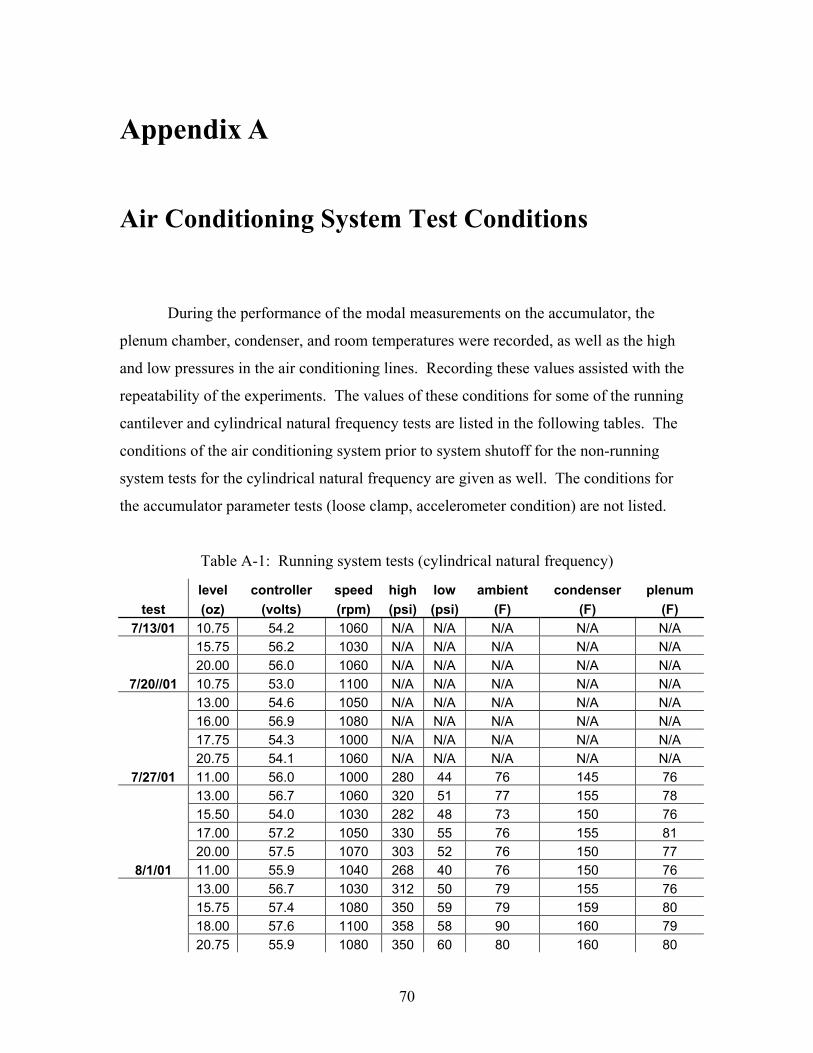
Appendix A

Air Conditioning System Test Conditions

During the performance of the modal measurements on the accumulator, the

plenum chamber, condenser, and room temperatures were recorded, as well as the high

and low pressures in the air conditioning lines. Recording these values assisted with the

repeatability of the experiments. The values of these conditions for some of the running

cantilever and cylindrical natural frequency tests are listed in the following tables. The

conditions of the air conditioning system prior to system shutoff for the non-running

system tests for the cylindrical natural frequency are given as well. The conditions for

the accumulator parameter tests (loose clamp, accelerometer condition) are not listed.

Table A-1: Running system tests (cylindrical natural frequency)

level controller speed high low ambient condenser plenum test (oz) (volts) (rpm) (psi) (psi) (F) (F) (F)

7/13/01 10.75 54.2 1060 N/A N/A N/A N/A N/A 15.75 56.2 1030 N/A N/A N/A N/A N/A 20.00 56.0 1060 N/A N/A N/A N/A N/A

7/20//01 10.75 53.0 1100 N/A N/A N/A N/A N/A 13.00 54.6 1050 N/A N/A N/A N/A N/A 16.00 56.9 1080 N/A N/A N/A N/A N/A 17.75 54.3 1000 N/A N/A N/A N/A N/A 20.75 54.1 1060 N/A N/A N/A N/A N/A

7/27/01 11.00 56.0 1000 280 44 76 145 76 13.00 56.7 1060 320 51 77 155 78 15.50 54.0 1030 282 48 73 150 76 17.00 57.2 1050 330 55 76 155 81 20.00 57.5 1070 303 52 76 150 77

8/1/01 11.00 55.9 1040 268 40 76 150 76 13.00 56.7 1030 312 50 79 155 76 15.75 57.4 1080 350 59 79 159 80 18.00 57.6 1100 358 58 90 160 79 20.75 55.9 1080 350 60 80 160 80

70

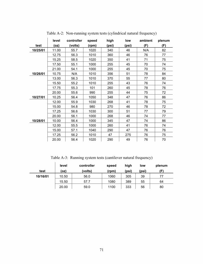
Table A-2: Non-running system tests (cylindrical natural frequency)

level controller speed high low ambient plenum test (oz) (volts) (rpm) (psi) (psi) (F) (F)

10/25/01 11.00 55.7 1020 340 46 N/A 82 12.75 56.3 1010 360 46 76 77 15.25 58.5 1020 350 41 71 75 17.50 55.1 1000 255 45 70 74 21.00 54.1 1000 255 45 70 75

10/26/01 10.75 N/A 1010 356 51 78 84 13.00 56.3 1010 370 55 77 80 15.50 55.2 1010 255 43 76 74 17.75 55.3 101 260 45 78 76 20.00 55.6 990 255 44 75 72

10/27/01 10.25 56.4 1050 348 47 76 86 12.00 55.9 1030 268 41 78 75 15.00 54.8 980 270 46 78 72 17.25 56.6 1030 300 51 77 79 20.00 56.1 1000 268 46 74 77

10/28/01 10.00 56.4 1000 345 47 74 86 12.00 55.5 1000 260 41 76 74 15.00 57.1 1040 290 47 76 76 17.25 56.2 1010 47 275 76 75 20.00 56.4 1020 290 49 76 70

Table A-3: Running system tests (cantilever natural frequency)

level controller speed high low plenum test (oz) (volts) (rpm) (psi) (psi) (F)

10/16/01 10.50 56.0 1060 305 39 77 15.50 57.7 1080 389 55 64 20.00 59.0 1100 333 56 80

71

Appendix B

Mode Shape of Cylinder

The mode shape of the accumulator bottle at the second studied natural frequency

used in the research to determine refrigerant level was addressed after refrigerant level

testing was completed. As described in Appendix C, the chance that the measured

natural frequency was a cylindrical mode and not a bending mode was very good

considering that the calculated natural frequencies for an axial-radial mode were lower

than for a bending mode. To clarify that the second natural frequency studied was

actually a cylindrical mode and not a bending mode, additional experimentation was

performed.

Modal analysis was performed on the accumulator bottle in the studied natural

frequency range of 1400 Hz. The laboratory test rig was empty of any R-134a

refrigerant, and the natural frequencies obtained experimentally were expected to a bit

higher than if the system had contained refrigerant due to the absence of the refrigerant

mass. The accelerometer was placed at the top of the accumulator on side A and hammer

impacts were performed at test point 5 on side A, side C, and side F of the accumulator.

An illustration of the test setup is shown in Figure B-1. Side C of the accumulator is

along the y-axis, and side A and side F are along the x-axis.

72

Figure B-1: Test setup for determining cylindrical mode

The obtained frequency response functions (FRFs) are shown in the following

figures: Figure B-2 for side A, Figure B-3 for side C, and Figure B-4 for side F. The

FRFs clearly show two natural frequencies in close proximity to one another. In the

research, the dominant natural frequency shown at 1480 Hz was used to determine the

amount of R-134a refrigerant in the system. Plotting the mode shape of the accumulator

at the studied natural frequency cannot be done from simply taking the imaginary

component and plotting. The proximity of the other natural frequency will affect the

components of the desired natural frequency resulting in an inaccurate mode shape

measurement. Therefore, for this natural frequency, the exact mode shape will not be

determined, but the type of mode shape will be determined qualitatively.

73

74

FigureB-2: Frequency response function for side A

FigureB-3: Frequency response function for side C

FigureB-4: Frequency response function for side F

The phase plots of the FRFs determine how the cylinder acts at cylindrical natural

frequency. Examining the phase from side A and side F indicates the direction of the

phase as being the same, signifying a negative imaginary component. This infers that

side A and side F of the accumulator are vibrating, or bending, in toward each other

simultaneously. The direction of the phase for side C is positive, signifying a positive

imaginary number. This indicates that side C is vibrating, or bending, outwards as the

sides on the orthogonal plane (side A and side F) vibrate inwards. From this data, the

cylinder can be described as vibrating in a radial-axial mode as shown in Figure B-5.

The determined cylindrical natural frequency mode could be the one shown in the figure

or one of a higher order.

Figure B-5: Determined cylindrical mode of accumulator

75

Appendix C

Analytical Natural Frequency

C.1 Analytical Natural Frequencies

Comparing analytical natural frequencies and theoretical mode shapes to the

experimentally measured natural frequencies help clarify the experimental results. To

calculate the natural frequencies, a model of the accumulator bottle was required. A

single degree of freedom system model was used to calculate the cantilever natural

frequency, and a continuous system model was used to calculate the cylindrical natural

frequencies. The theory for single degree of freedom and continuous systems can be

found in further detail in Inman [2001] and Blevins [1979].

C.2 Cantilever Natural Frequency

From experimentation, the first discovered natural frequency of the accumulator

bottle was found to be in the low frequency region of 45 Hz. Because this natural

frequency was relatively lower than the next measured natural frequency in the kHz

region, it was speculated that at low frequencies, the accumulator bottle system vibrates

in the transverse direction as single degree of freedom system. In this single degree of

freedom system, the accumulator bottle acts as a mass at the end of the inlet line, which

acts as a cantilevered beam. The concept of the discussed transverse vibration of a beam

of length l with a tip mass m is illustrated in Figure C-1.

76

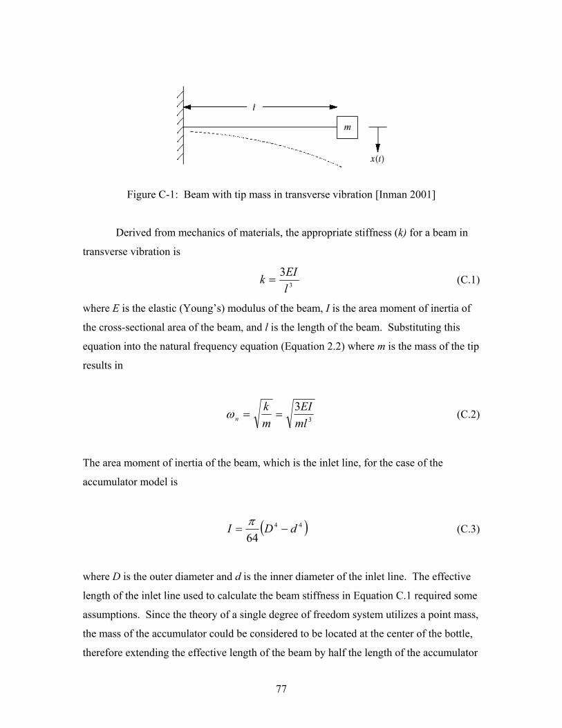
Figure C-1: Beam with tip mass in transverse vibration [Inman 2001]

Derived from mechanics of materials, the appropriate stiffness (k) for a beam in

transverse vibration is

3

3lEIk = (C.1)

where E is the elastic (Young’s) modulus of the beam, I is the area moment of inertia of

the cross-sectional area of the beam, and l is the length of the beam. Substituting this

equation into the natural frequency equation (Equation 2.2) where m is the mass of the tip

results in

3

3mlEI

mk

n ==ω (C.2)

The area moment of inertia of the beam, which is the inlet line, for the case of the

accumulator model is

( 44

64dDI −= )π

(C.3)

where D is the outer diameter and d is the inner diameter of the inlet line. The effective

length of the inlet line used to calculate the beam stiffness in Equation C.1 required some

assumptions. Since the theory of a single degree of freedom system utilizes a point mass,

the mass of the accumulator could be considered to be located at the center of the bottle,

therefore extending the effective length of the beam by half the length of the accumulator

77

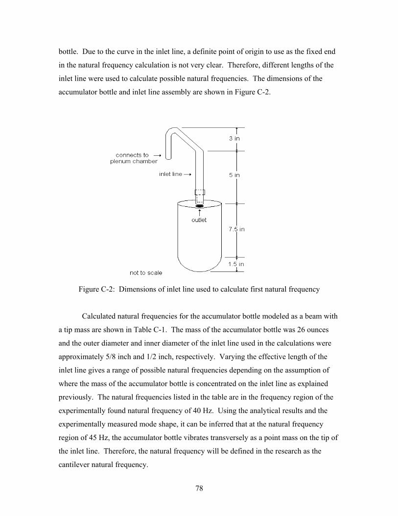
bottle. Due to the curve in the inlet line, a definite point of origin to use as the fixed end

in the natural frequency calculation is not very clear. Therefore, different lengths of the

inlet line were used to calculate possible natural frequencies. The dimensions of the

accumulator bottle and inlet line assembly are shown in Figure C-2.

Figure C-2: Dimensions of inlet line used to calculate first natural frequency

Calculated natural frequencies for the accumulator bottle modeled as a beam with

a tip mass are shown in Table C-1. The mass of the accumulator bottle was 26 ounces

and the outer diameter and inner diameter of the inlet line used in the calculations were

approximately 5/8 inch and 1/2 inch, respectively. Varying the effective length of the

inlet line gives a range of possible natural frequencies depending on the assumption of

where the mass of the accumulator bottle is concentrated on the inlet line as explained

previously. The natural frequencies listed in the table are in the frequency region of the

experimentally found natural frequency of 40 Hz. Using the analytical results and the

experimentally measured mode shape, it can be inferred that at the natural frequency

region of 45 Hz, the accumulator bottle vibrates transversely as a point mass on the tip of

the inlet line. Therefore, the natural frequency will be defined in the research as the

cantilever natural frequency.

78

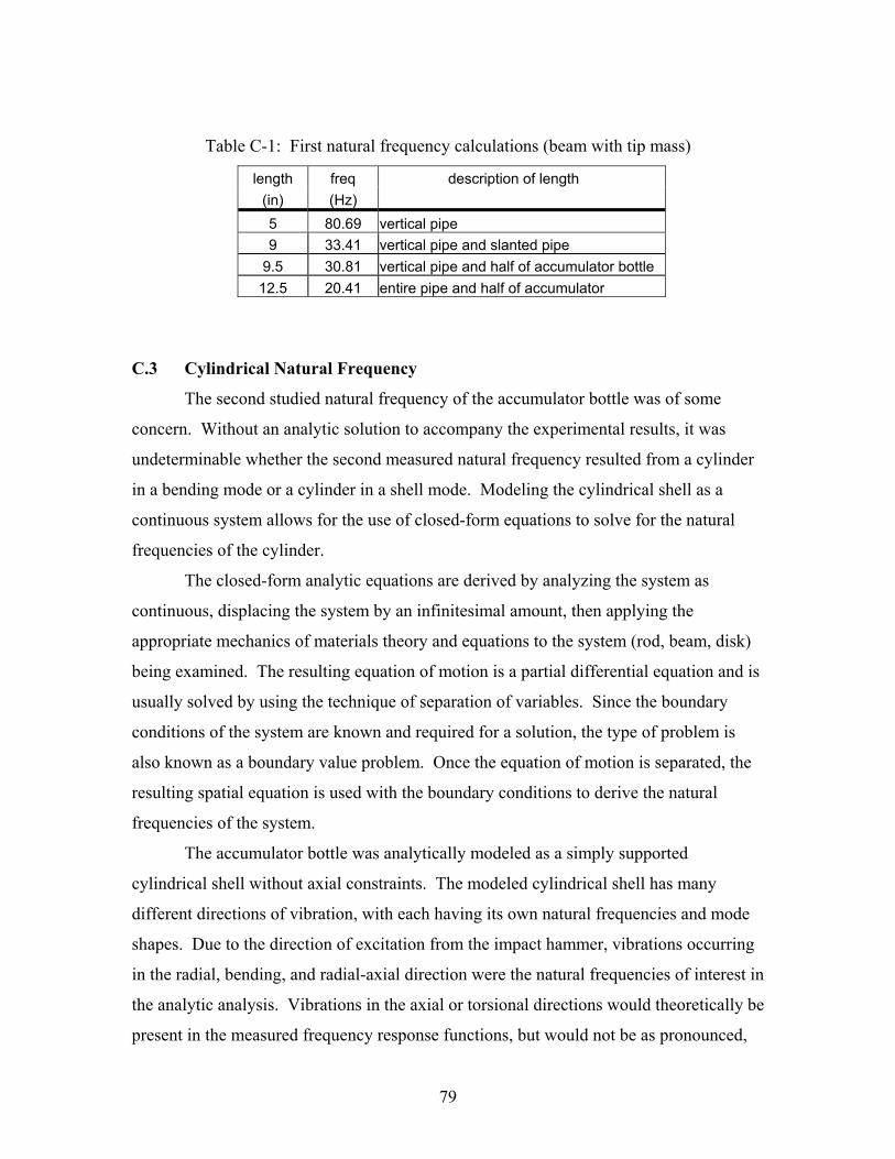
Table C-1: First natural frequency calculations (beam with tip mass)

length freq description of length (in) (Hz) 5 80.69 vertical pipe 9 33.41 vertical pipe and slanted pipe

9.5 30.81 vertical pipe and half of accumulator bottle 12.5 20.41 entire pipe and half of accumulator

C.3 Cylindrical Natural Frequency

The second studied natural frequency of the accumulator bottle was of some

concern. Without an analytic solution to accompany the experimental results, it was

undeterminable whether the second measured natural frequency resulted from a cylinder

in a bending mode or a cylinder in a shell mode. Modeling the cylindrical shell as a

continuous system allows for the use of closed-form equations to solve for the natural

frequencies of the cylinder.

The closed-form analytic equations are derived by analyzing the system as

continuous, displacing the system by an infinitesimal amount, then applying the

appropriate mechanics of materials theory and equations to the system (rod, beam, disk)

being examined. The resulting equation of motion is a partial differential equation and is

usually solved by using the technique of separation of variables. Since the boundary

conditions of the system are known and required for a solution, the type of problem is

also known as a boundary value problem. Once the equation of motion is separated, the

resulting spatial equation is used with the boundary conditions to derive the natural

frequencies of the system.

The accumulator bottle was analytically modeled as a simply supported

cylindrical shell without axial constraints. The modeled cylindrical shell has many

different directions of vibration, with each having its own natural frequencies and mode

shapes. Due to the direction of excitation from the impact hammer, vibrations occurring

in the radial, bending, and radial-axial direction were the natural frequencies of interest in

the analytic analysis. Vibrations in the axial or torsional directions would theoretically be

present in the measured frequency response functions, but would not be as pronounced,

79

and therefore, not performed in the analysis. Figure C-3 illustrates the modes examined

in the analytic analysis with the displacements indicated in dashed lines.

Figure C-3: Modes of a cylinder analyzed in the analysis [adapted from Blevins 1979]

The equation used to find the various natural frequencies (Hz) of a simply

supported cylindrical shell without axial constraints is

( )2/1

212

−

=νµπ

λω E

Rij

ij (C.4)

where R is the outside radius of the cylinder (the approximate accumulator radius was

1.75 inches), E is the elastic (Young’s) modulus of the material, µ is the mass density of

the cylinder material, and ν is Poisson’s ratio. The values used for the variables i and j

depend on the type of vibration (radial, bending), being analyzed. Illustrations of modes

of the i and j variables are shown in Figure C-4. The variable λij is a function of the type

of vibration natural frequency of interest and the boundary conditions of the cylinder.

The derivation of the closed-form equations and the equations for lambda can be found in

Chapter 12 of Blevins [1979].

80

Figure C-4: Axial and circumferential modes [adapted from Blevins 1979]

The first three natural frequencies for radial, bending, and radial-axial vibration of

the modeled accumulator were calculated and are shown in Table C-2. Examining the

results indicates the radial-axial natural frequency occurs before any other type of

vibration. The natural frequency experimentally found at 1400 Hz is more likely to be a

radial-axial natural frequency than a radial or bending natural frequency. Because of the

discrepancy between the experimental and analytical natural frequencies, accurately

determining the type of mode shape of the accumulator at the measured cylindrical

natural frequency required some additional testing and is detailed in Appendix B.

Table C-2: Analytical natural frequencies for cylindrical modes

radial bending radial-axialfreq 1 (Hz) 19,245 7,901 3,037 freq 2 (Hz) 19,245 31,648 5,992 freq 3 (Hz) 19,245 71,207 9,740

Analytically, the natural frequency values are larger than the experimental values,

and this is to be expected. Some possibilities for this difference involve the derivation of

81

the natural frequency equations for the theoretical cylinder. The theoretical cylinder is

hollow, whereas the inside of the actual accumulator bottle is not. Containing a desiccant

bag, stand pipe, and possibly more, the increased mass more than likely causes the

experimentally obtained natural frequencies to be lower than the analytically obtained

natural frequencies.

82

Vita

Eric C. Stasiunas was born on April 20, 1978 in Nashville, Tennessee. Raised in Music

City USA, Eric graduated from McGavock High School in 1996, and proceeded to attend

Tennessee Technological University in the small town of Cookeville, Tennessee.

Choosing mechanical engineering as his major because it looked more fun than electrical,

chemical, or civil engineering, Eric received his Bachelor of Science Degree in December

2000. Eric’s professors at TTU suggested attending graduate school a few times during

his senior year. During his last semester as an undergraduate, Eric decided that graduate

school may not be as horrible as it sounds, and decided to attend Virginia Polytechnic

Institute in the even smaller town of Blacksburg. It was there that he discovered that the

subject of vibrations is not only decipherable, but it actually makes sense and has

millions of applications in the “real world” that Eric kept hearing about. This newfound

appreciation for vibrations was welcome, since Eric’s thesis project involved vibrations.

Eric also learned a valuable trade relating to vibrations, modal analysis. This allowed

him to find a job out in New Mexico at Sandia National Laboratory where he will

continue doing modal analysis in the hope of one day obtaining a coherence of 1.

83