Using Taguchi Method to Optimize Welding Pool of Dissimilar

Laser Welded Components

E. M. Anawa and A. G. Olabi and

School of Mechanical & Manufacturing Eng., Dublin City University, Dublin 9, Ireland

ezzeddin.hassan2 @mail.dcu.ie, abdul.olabi@dcu.ie

ABSTRACT

In the present work CO2 continuous laser welding process was successfully applied and

optimized for joining a dissimilar AISI 316 stainless steel and AISI 1009 low carbon steel

plates. Laser power, welding speed, and defocusing distance combinations were carefully

selected with the objective of producing welded joint with complete penetration, minimum

fusion zone size and acceptable welding profile. Fusion zone area and shape of dissimilar

austenitic stainless steel with ferritic low carbon steel were evaluated as a function of the

selected laser welding parameters. Taguchi approach was used as statistical design of

experiment (DOE) technique for optimizing the selected welding parameters in terms of

minimizing the fusion zone. Mathematical models were developed to describe the influence of

the selected parameters on the fusion zone area and shape, to predict its value within the limits

of the variables being studied. The result indicates that the developed models can predict the

responses satisfactorily.

Keywords: Dissimilar material, Welding fusion zone, CO2 continuous laser welding, Taguchi

approach.

1. INTRODUCTION

The demand for producing joints of dissimilar materials is continuously increasing

due to their advantages, which can provide appropriate mechanical properties and good

cost reduction. There are many issues/problems associated with the joining of dissimilar

materials, depending on the materials being joined and process employed. In the welding

of dissimilar materials different factors should be considered such as; (a) carbon migration

from the higher carbon containing alloy to the relatively lower carbon alloy steels,

especially those which are highly alloyed, (b) the differences in thermal expansion

coefficients, resulting in differences in thermal residual stresses across the different

weldment regions, (c) difficulty in executing the post weld heat treatment, especially in

combinations wherein either of the materials being joined is susceptible to undesirable

precipitation at elevated temperatures and (d) electrochemical property variations in the

weldment, resulting in environmentally assisted problems [1]. Dissimilar welding of

austenitic stainless steel with ferritic low carbon steel (A/F) is faced with the coarse grains

phenomena in the weld zone and heat affected zone of fusion welds leading to low

toughness and ductility due to the absence of phase transformation [2]. Laser welding has

become an important industrial process because of its advantages as a bonding process

over the other widely used joining techniques. Laser welding is characterized by parallel-

sided fusion zone, narrow weld width and high penetration. These advantages come from

its high power density, which make the laser welding one of the keyhole welding processes

[3, 4]. Welding quality is strongly characterized by the weld bead geometry. Due to that

the weld bead geometry plays an important role in determining the mechanical properties

of the welded joints. Therefore, it is very essential the selection of the welding process

parameters for obtaining optimal weld bead geometry. [5-7]. Design of Experiment (DOE)

and statistical techniques are widely used to optimize process parameters. Many researches

were conducted to identify the optimal process input parameters. The most important input

laser welding parameters which would control the welding quality outputs are laser power,

welding speed and focus position [8-12]. Taguchi method is one of the optimization

techniques which could be applied to optimize input welding parameters. Optimization of

process parameters is the key step in the Taguchi method in achieving high quality without

increasing the cost. This is because optimization of process parameters can improve

performance characteristics. The optimal process parameters obtained from the Taguchi

method are insensitive to the variation of environmental conditions and other noise factors

[10]. Basically, classical process parameter design is complex and not easy to use. This is

particularly true when the number of the process parameters increases, leading to a large

number of experiments have to be carried out. To solve this task, Taguchi method with a

special design of orthogonal arrays can be used to study the entire process parameter space

with a small number of experiments only [14].

The obtained results from Taguchi method are insensitive to the variation of

environmental conditions and other noise factors. The optimal combination of the process

parameters can then be predicted [15].

This work is concerned with evaluating the effects of welding parameters on the total

weld pool fusion area as a welding output and considered as a response ‘A’ of A/F joints

and the prediction of the optimal combinations of the welding parameters with an objective

of minimizing it. Welding widths at the specimen surface and at the middle depth also

were studied as responses ‘W1’ and ‘W2’ respectively to detect the effect of the selected

welding parameters on the welding pool shape. The welding parameters and the listed

responses will be considered as inputs and outputs respectively for Taguchi analysis. Fig. 1

shows the positions of responses on the specimen.

2. EXPERIMENTAL DESIGN AND PROCEDURE

Taguchi approach was used for designing the experiments, L-25 orthogonal array

was applied which composed of 3 columns and 25 rows, which mean that 25 experiments

were carried out. Design of experiment was selected based on a three welding parameters

with five levels each. The selected welding parameters for this study are: welding power,

welding speed and focus point position. Table 1 show the laser input variables and

experiment design levels. The Taguchi method was applied to the experimental data using

statistical softwares “Design-expert 7” and “MINITAB 13”. The S/N ratio for each level of

process parameters is computed based on the S/N analysis. Regardless of the category of

the quality characteristic, a lower S/N ratio corresponds to a better quality characteristic.

Therefore, the optimal level of the process parameters is the level with the lowest S/N

ratio. Furthermore, a statistical analysis of variance (ANOVA) is performed for each

response individually to see which process parameters are statistically significant. The

optimal combination of the process parameters can then be predicted.

The materials employed in this investigation were plates of AISI 316 stainless steel

and AISI 1009 milled carbon steel in dimensions of 160 mm x 80 mm x 2 mm each were

used as work-pieces materials. The typical chemical compositions of the received materials

are shown in Table 2. The joints were produced using CO2 LBW (laser beam welding) at a

maximum laser power of 1.5 kW with welding conditions as described in Table 1.

Specimens for the metallographic examinations were prepared by polishing successively in

120, 240, 500 and 800emery grits, followed by a final disc polishing using 9, 6 and 3 μm

diamond slurry. The carbon steel side of the weldment was etched in 4% Nital, and the rest

of the regions of the weldment were etched in a solution containing 20 ml hydrochloric

acid, 1.0 g sodium meta bisulphate and 100 ml distilled water. Also, an electrolytic etching

in 10% (w/o) oxalic acid was employed to reveal the features of weld metal and the

evolved interfaces. The average of at least three results of welding pool area was measured

for each sample. Fig. 2, Shows the effect of the welding parameters on the responses (A,

W1, W2) of some of selected experiments listed in Table 3, and the variation on weld bead

geometry. The experimental measured responses are presented in Table 3.

3. RESULTS AND DISCUSSION

The area of the fusion welding zone (A) was measured by using the transverse

sectioned specimens, the optical microscope and image analyser software. Using the same

procedure the welding pool width at surface (W1) and the welding pool width at the

middle depth (W2) of the specimens also were measured and analysed as process

responses. The measured responses are listed in Table 3 and exhibited in Fig. 1. Design

expert 7 software had been used for analysing the measured responses. The fit summary

output indicates that the models developed are statistically significant for the prediction of

the responses therefore they will be used for further analysis. It has been seen that the

welding pool and penetration are controlled by the rate of heat input, which is a function of

laser power and welding speed [16]. But the focusing parameter is mostly affecting the

weld pool surface width.

3.1 Orthogonal Array Experiment

In the present study, the interaction between the welding parameters is neglected.

Therefore, degrees of freedom owing to the three sets of five-level welding process

parameters were analysed. The degrees of freedom for the orthogonal array should be

greater than or at least equal to those for the process parameters. In this study, an L25

orthogonal array with three columns and 25 rows was used. This array has twelve degrees

of freedom and it can handle five-level process parameters. Twenty-five experiments were

required to study the welding parameters using L25 orthogonal array. The experimental

layout for the welding process parameters using the L25 orthogonal array is shown in

Table 3 and the responses for signal-to-noise ratio S/N are presented in Table 4.

3.2 The Signal-to-Noise (S/N) Ratio Analysis

In order to evaluate the influence of each selected factor on the responses: The

signal-to-noise ratios S/N for each control factor had to be calculated. The signals have

indicated that the effect on the average responses and the noises were measured by the

influence on the deviations from the average responses, which would indicate the

sensitiveness of the experiment output to the noise factors. The appropriate S/N ratio must

be chosen using previous knowledge, expertise, and understanding of the process. When

the target is fixed and there is a trivial or absent signal factor (static design), it is possible

to choose the S/N ratio depending on the goal of the design. In this study, the S/N ratio

was chosen according to the criterion the-smaller-the-better, in order to minimize the

responses. The S/N ratio for the-smaller-the-better target for all the responses was

calculated as follows:

nyNS /log10/ 2

10

Where: y is the average measured fusion area, n the repetitions, in this study

=25

Using the above-presented data with the selected above formula for calculating S/N,

the Taguchi experiment results are summarised in Table 4 and presented in Fig. 3, which

were obtained by means of MINITAB 13 statistical software. It can be noticed from this

Fig. that the S/N plot, that the travel speed ‘S’ is the most important factor affecting the

responses; the minimum value of response is at the highest level of ‘S’. Laser power has a

lower relevant effect. While the focus point position plots show the lowest effect among

those factors. Main effects plot for S/N ratios suggest that those levels of variables would

minimise the weld pool dimensions, also were robust against variability due to noises as

presented in Fig. 3.

3.3 Analysis of Variance

The purpose of the analysis of variance (ANOVA) is to investigate which welding

process parameters significantly affect the quality characteristic. This is accomplished by

separating the total variability of the S/N ratios, which is measured by the sum of the

squared deviations from the total mean of the S/N ratio, into contributions by each welding

process parameter and the error [17, 18]. The test for significance of the regression model,

the test for significance on individual model coefficients and the lack-of- fit test were

performed using Design Expert 7 software.

Step-wise regression method; which eliminates the insignificant model terms

automatically was applied and exhibited in ANOVA Tables 5-7 for the reduced quadratic

model. ANOVA Tables summarise the analysis of three variances of the responses and

show the significant models.

3.3.1 ANOVA Outputs

F Value: Test for comparing model variance with residual (error) variance. When

the variances are close to each other, the ratio will be close to one and it is less likely that

any of the factors have a significant effect on the response. F Value is calculated by term

mean square divided by residual mean square. Prob > F: Probability of seeing the observed

F value if the null hypothesis is true (there is no factor effect). If the Prob>F value is very

small (less than 0.05) then the individual terms in the model have a significant effect on the

response. Precision of a parameter estimate is based on of the number of independent

samples of information which can be determined by degree of freedom (df). The degree of

freedom equals to the number of experiments minus the number of additional parameters

estimated for that calculation. The same tables show also the other adequacy measures R2,

adjusted R2,

adequacy precision R

2 and predicted R

2 for each response. The entire adequacy

measures were close to 1, which are reasonable and indicate adequate models. The

adequate precision compares the range of the predicted value at the design points to the

average predicted error. In this study the value of adequate precision are significantly

greater than 4. The adequate precision ratio above 4 indicates adequate model

discrimination.

The analysis of variance indicates that for the welding pool area (A) model, the

main effect was the welding speed (S), the second order effect was the laser power (P) and

the two level interaction of laser welding and welding speed (P and S) are the most

significant model parameters. Secondly for the welding pool width at the work piece

surface (W1) model, the analysis indicated that there is a linear relationship between the

main effects of the three parameters. Also, in case of welded pool width at the middle of

work piece (W2) model the main effect of laser power (P), welding speed (S), focused

position (F), the second order effect of welding speed (S2) are significant model terms.

However, the main effect of welding speed (S) is the most important factor influent the

welding pool.

The final mathematical models in terms of actual factors as determined by design

expert software are shown below.

3.3.2 Final Equations in Terms of Actual Factors:

A = -3.681 + 6.084* P +6.479E-003* S -7.028E-003 * P * S ( 1 )

W1 = +5.757 -1.922* P -1.878E-003 * S + 3.260* F – 2.955* P * F ( 2 )

W2 = +2.010 +0.218* P -3.696E-003* S -0.152 * F +2.006E-006* S2 ( 3 )

3.4 Model Validation

The final step is to predict and verify the improvement of the response using the

optimal level of the welding process parameters.

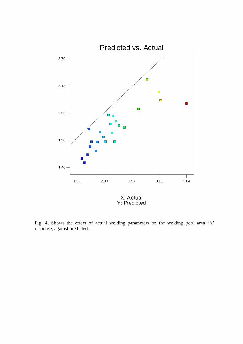
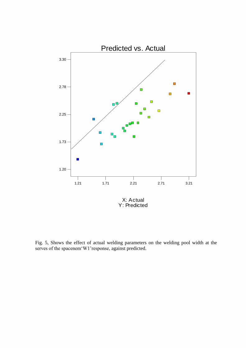
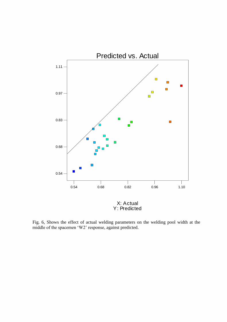
Figs. 4-6 show the relationship between the actual and predicted values of A, W1, and

W2, respectively. These figures indicate that the developed models are adequate

because the residuals in prediction of each response are negligible, since the residuals

tend to be close to the diagonal line. Furthermore, to verify the satisfactoriness of the

developed models, three confirmation experiments were carried out using new test

conditions at optimal parameters conditions, obtained using the design expert software.

Table 8 expresses the best ten parameters combination which were predicted using

software. First value indicates the lowest responses and so on. The A, W1 and W2 of

the validation experiments were selected from Table 8. Table 9 summarizes the

experiments conditions, the actual experimental values, the predicted values and the

percentages of error. It could be concluded that the models developed could predict the

responses with a very small error. A, W1 and W2 were greatly improved through this

optimization.

4. EFFECT OF THE PARAMETERS ON RESPONSES

The reason for predicting the welding pool geometry is to develop a model which

would include the optimizations step for future work. Fig. 7 contour graph shows the effect

of S and P on the total welding pool area (A) at F = −0.5 mm. Fig. 8 contour graph shows

the effect of P and F on the welding pool width at the work piece surface (W1) at S = 750

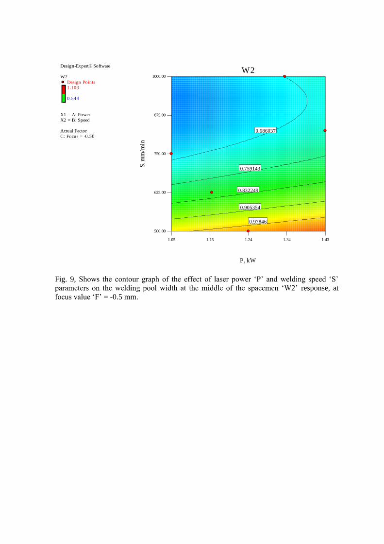
mm/min. Fig. 9 contour graph shows the effect of P and S on the welding pool width at the

middle of work piece (W2) at F = - 0.5.

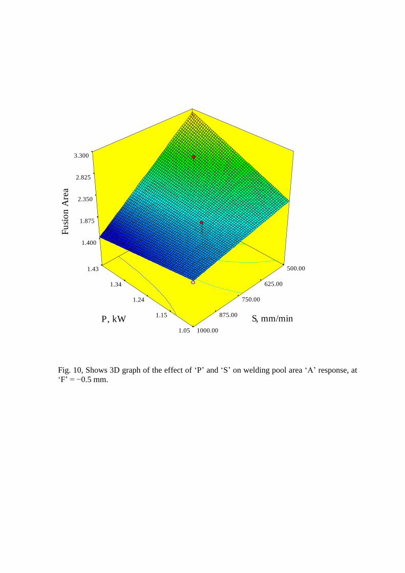
4.1 Welding Pool Area ‘A’

In the present study the fusion area (welding pool) ‘A’ of dissimilar joints between

stainless steel and low carbon steel was measured and plotted in 3D graph as presented in

Fig. 10. This Fig. shows that the welding speed has the most significant effect on the

process. The increase in welding speed ’S’ rate, lead to the reduction of the fusion area of

the welding pool. When welding speed equal maxima at 1000 mm/min, as presented in

Table 3, the fusion area is minima and equals 1.598 mm2 which present the best achieved

results. It is also noted that changes in the laser power ‘P’ rate would lead to change the

fusion area value. By increasing laser power the fusion area tends to decrease up to lower

value at laser power equals 1.15 kW then start to trend-on up to laser power equal to 1.33

kW. Further increases of laser power value result in the fusion area increasing again. The

fusion area has the minimum value at laser power equal 1.33 kW these results are shown in

Fig. 2 and 3. From Fig. 3 it’s clear that the focusing position ‘F’ has insignificant effect on

the welding pool, where by changing the focusing position the welding pool will not be

consequentially changed and this effect is ensured in Table 4 in which the focusing

position has the greater value (rank = 3) in S/N ratio.

4.2 Welding Pool Width at the Work Piece Surface (W1).

The results and the model obtained for the response indicate that the S and F are the

most important factors affecting W1 value. An increase in S leads to a decrease in W1.

This is due to the laser beam traveling at high speed over the welding line when S is

increased. Therefore the heat input decreases leading to less volume of the base metal

being melted, consequently the width of the welded zone decreases. Moreover, defocused

beam, which mean wide laser beam results in spreading the laser power onto wide area.

Therefore, wide area of the base metal will be melted leading to an increase in W1 or vice

versa. The result shows also that P contributes secondary effect in the response width

dimensions. Increases in P will results in slight increases in W1, due to the increase in the

power density. Fig. 11 shows 3D plots for the effect of process parameters on the W1

width.

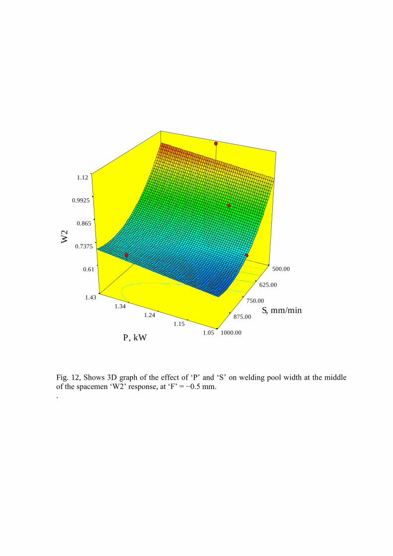
4.3 Welding Pool Width at the Middle of the Work Piece (W2)

From the results it is clear that the three parameters are significantly affecting the W2

value. Using a focused beam results in an increase in the power density, which indicates

that the heat will be localize in a small metal portion, resulting in an increase in the power

density leading to increasing W2 value. The model shows that the response is proportioned

inversely with F. The result shows that the changes in F parameter effects W1, W2 and

didn’t effect A. This may be interpreted that as F decreased, W1 increasing, W2 decreased

and vice versa, so the total area A will not be effected by changing F. The increase in P

leads to an increase in the heat input, therefore, more molten metal and consequently wider

W2 will be achieved. However, the idea is reversed in the case of S effect, because the S is

inversely proportioned with the heat input. Fig. 12 shows 3D plots to present the effect of

process parameters on the W2 value.

5. CONCLUSION

The following points can be concluded from this study:

i) Using Laser welding could produce a small welding pool and a narrow HAZ.

ii) Welding speed has the stronger effect on the fusion area size among the

selected parameters; which is proportional inversely with responses.

iii) Laser power has strong effect on fusion area. By changing the P value the

response will be changed dramatically, so the P value should be carefully

selected. The focusing position parameter has insignificant effect on the total

weld pool size.

iv) The model developed can be adequately in predicting the responses within the

factors domain.

ACKNOWLEDGEMENT

Libyan educational ministry is gratefully acknowledged for the financial support of

this research. Technical support from Mr. Martin Johnson and Mr. Michael May and

Dublin City University are also gratefully acknowledged.

REFERENCES:

[1] P. Bala Srinivasan, V. Muthupandi, W. Dietzel, V. Sivan, An assessment of impact

strength and corrosion behavior of shielded metal arc welded dissimilar weldments

between UNS 31803 and IS 2062 steels, Materials and Design 27 (2006) 182–191.

[2] V.V Satyanarayana, G. Madhusudhan Reddy, T. Mohandes, Journal of Materials

Processing Technology, 160 (2005) 128-137.

[3] E. M. Anawa, A. G. Olabi and M. S. J. Hashmi, Optimization of ferritic/Austenitic

laser welded components, presented at AMPT2006 Inter. Conf. July 30 to 3 Aug.,

2006, Las Vegas, Nevada, USA, 2006, p. 04 325.

[4] W.M. Steen, Journal of Laser Applications , October 1999 , Volume 11, Issue 5, pp.

216-219 Springer, London, 1991.

[5] Y. M. Zhang, R. Kovacevic and L. Li, "Characterization and realtime measurement of

geometrical appearance of the weld pool", International Journal of Machine Tools

and Manufacture, 36(7), pp. 799-816, 1996.

[6] C. E. Bull, K. A. Stacey and R. Calcraft, "On line weld monitoring using ultrasonic",

Journal of Non-destructive Testing, 35(2), pp. 57- 64, 1993.

[7] Y. S. Tarng and W. H. Yang, Optimisation of the Weld Bead Geometry in Gas

Tungsten Arc Welding by the Taguchi Method, J Adv Manuf Technol (1998)

14:549-554

[8] K. Y. Benyounis, A. G. Olabi and M. S. J. Hashmi, Estimation of mechanical

properties of laser welded joints using RSM, International Manufacturing

Conference (2005) 565- 571.

[9] Y. S. Tarng, S. C. Juang and C. H. Chang, The use of grey-based Taguchi methods to

determine submerged arc welding process parameters in hard facing, Journal of

Materials Processing Technology, Volume 128, Issues 1-3, 6 October 2002, Pages 1-

6.

[10] Lung Kwang Pan, Che Chung Wang, Ying Ching Hsiao and Kye Chyn Ho,

Optimization of Nd:YAG laser welding onto magnesium alloy via Taguchi analysis,

Optics & Laser Technology, Volume 37, Issue 1, February 2005, Pages 33-42.

[11] Hyoung-Keun Lee, Hyon-Soo Han, Kwang-Jae Son and Soon-Bog Hong,

Optimization of Nd: YAG laser welding parameters for sealing small titanium tube

ends, Materials Science and Engineering: A, Volume 415, Issues 1-2, 15 January

2006, Pages 149-155.

[12] E. M. Anawa and A. G. Olabi, Effect of laser welding conditions on toughness

of dissimilar welded components, J. of Applied Mechanics and Materials, Vol.

5-6, 2006, 375-380.

[13] Y.S. Tarng, S.C. Juang, C.H. Chang, The use of grey-based Taguchi methods to

determine submerged arc welding process parameters in hard facing, Journal of

Materials Processing Technology 128 (2002) 1–6.

[14] D.C. Montgomery, Design and Analysis of Experiments, Wiley, Singapore, 1991.

[15] E. M. Anawa, A. G. Olabi and M. S. J. Hashmi, Application of Taguchi Method to

Optimize Dissimilar Laser Welded Components, presented at 23rd International

Manufacturing Conference 30th Aug. to 1st Sep., 2006, Belfast, UK, p. 241-248.

[16] A.G. Olabi , G. Casalino, K.Y. Benyounis, M.S.J. Hashmi , An ANN and Taguchi

algorithms integrated approach to the optimization of CO2 laser welding, Advances

in Engineering Software 37 (2006) 643–648.

[17] S.C. Juang, Y.S. Tarng, Process parameter selection for optimizing the weld pool

geometry in the tungsten inert gas welding of stainless steel, Journal of Materials

Processing Tec Processing Technology, 160 (2005) 128-137.

[18] K.Y. Benyounis, A.G. Olabi, M.S.J. Hashmi, Effect of laser welding parameters on

the heat input and weld-bead profile, Journal of Materials Processing Technology

164–165 (2005) 978–985.

List of tables:

1. Table 1 Process parameters and design levels used.

2. Table 2 Chemical composition of the materials (wt %).

3. Table 3 Experimental assignments, responses, and S/N ratio.

4. Table 4 Responses for signal-to-noise ratio (S/N).

5. Table 5 ANOVA for A response model.

6. Table 6 ANOVA for W1 response model.

7. Table 7 ANOVA for W2 response model.

8. Table 8 the best parameters combinations for greater responses.

9. Table9 Confirmation experiments and base metal responses.

List of figures:

1. Fig. 1, Shows the responses position on the work piece.

2. Fig. 2, Shows the effect of the welding parameters on the responses (A, W1,

W2), and the variation on weld bead geometry

3. Fig. 3, Effects plot for S/N ratio of the responses.

4. Fig. 4, Shows the effect of actual welding parameters on A response against

predicted.

5. Fig. 5, Shows the effect of actual welding parameters on W1 response against

predicted.

6. Fig. 6, Shows the effect of actual welding parameters on W2 response against

predicted.

7. Fig. 7, Contour graph shows the effect of P and S parameters on the response A.

8. Fig. 8, Contour graph shows the effect of P and F parameters on the response

W1.

9. Fig. 9, Contour graph shows the effect of P and S parameters on the response

W2.

10. Fig. 10, 3D graph shows the effect of P and S on A response at F = −0.5 mm.

11. Fig. 11, 3D graph shows the effect of P and S on W1 response at F = −1 mm.

12. Fig. 12, 3D graph shows the effect of P and S on W2 response at F = −1 mm.

Table 1 Process parameters and design levels used

Variables Code Unit Level 1 Level 2 Level 3 Level 4 Level 5

Laser Power P kW 1.05 114.9 1.24 1.33 1.43

Welding Speed S mm/min 500 625 750 850 1000

Focus F mm -1 -0.75 -0.5 -0.25 0

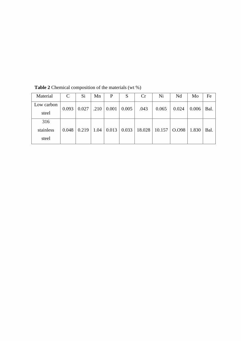
Table 2 Chemical composition of the materials (wt %)

Material C Si Mn P S Cr Ni Nd Mo Fe

Low carbon

steel 0.093 0.027 .210 0.001 0.005 .043 0.065 0.024 0.006 Bal.

316

stainless

steel

0.048 0.219 1.04 0.013 0.033 18.028 10.157 O.O98 1.830 Bal.

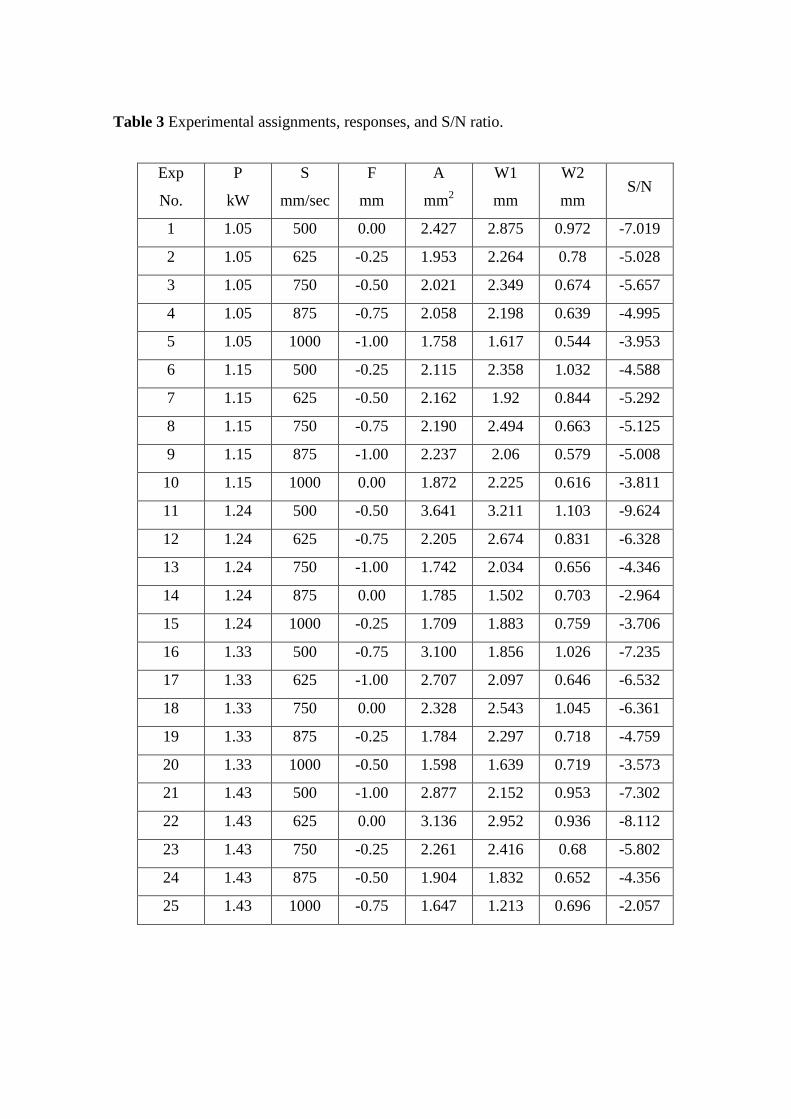
Table 3 Experimental assignments, responses, and S/N ratio.

Exp

No.

P

kW

S

mm/sec

F

mm

A

mm2

W1

mm

W2

mm S/N

1 1.05 500 0.00 2.427 2.875 0.972 -7.019

2 1.05 625 -0.25 1.953 2.264 0.78 -5.028

3 1.05 750 -0.50 2.021 2.349 0.674 -5.657

4 1.05 875 -0.75 2.058 2.198 0.639 -4.995

5 1.05 1000 -1.00 1.758 1.617 0.544 -3.953

6 1.15 500 -0.25 2.115 2.358 1.032 -4.588

7 1.15 625 -0.50 2.162 1.92 0.844 -5.292

8 1.15 750 -0.75 2.190 2.494 0.663 -5.125

9 1.15 875 -1.00 2.237 2.06 0.579 -5.008

10 1.15 1000 0.00 1.872 2.225 0.616 -3.811

11 1.24 500 -0.50 3.641 3.211 1.103 -9.624

12 1.24 625 -0.75 2.205 2.674 0.831 -6.328

13 1.24 750 -1.00 1.742 2.034 0.656 -4.346

14 1.24 875 0.00 1.785 1.502 0.703 -2.964

15 1.24 1000 -0.25 1.709 1.883 0.759 -3.706

16 1.33 500 -0.75 3.100 1.856 1.026 -7.235

17 1.33 625 -1.00 2.707 2.097 0.646 -6.532

18 1.33 750 0.00 2.328 2.543 1.045 -6.361

19 1.33 875 -0.25 1.784 2.297 0.718 -4.759

20 1.33 1000 -0.50 1.598 1.639 0.719 -3.573

21 1.43 500 -1.00 2.877 2.152 0.953 -7.302

22 1.43 625 0.00 3.136 2.952 0.936 -8.112

23 1.43 750 -0.25 2.261 2.416 0.68 -5.802

24 1.43 875 -0.50 1.904 1.832 0.652 -4.356

25 1.43 1000 -0.75 1.647 1.213 0.696 -2.057

Table 4 Responses for signal-to-noise ratio (S/N).

levels 1 2 3 4 5 Delta Rank

P, kW -6.49 -6.52 -6.98 -7.22 -6.15 1.07 2

S, mm/min -8.89 -7.59 -6.43 -5.78 -4.68 4.21 1

F, mm -6.91 -6.82 -5082 -6074 -7.09 1.27 3

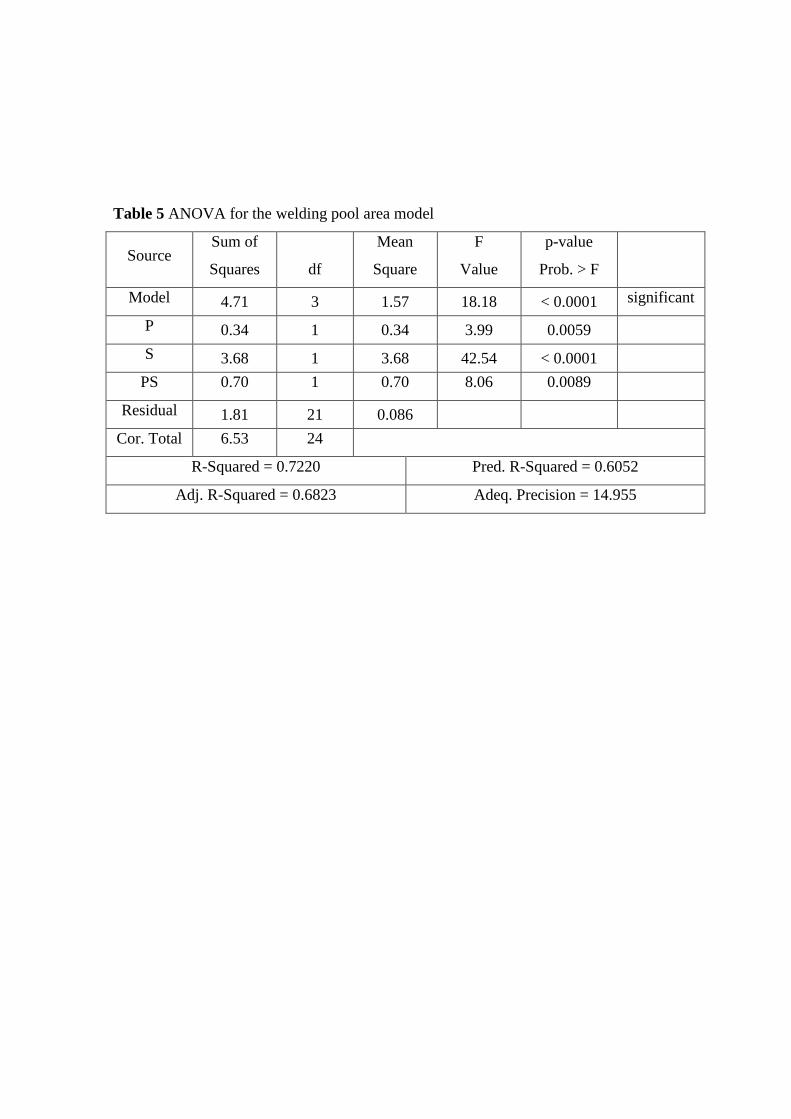
Table 5 ANOVA for the welding pool area model

Source Sum of

Squares

df

Mean

Square

F

Value

p-value

Prob. > F

Model 4.71 3 1.57 18.18 < 0.0001 significant

P 0.34 1 0.34 3.99 0.0059

S 3.68 1 3.68 42.54 < 0.0001

PS 0.70 1 0.70 8.06 0.0089

Residual 1.81 21 0.086

Cor. Total 6.53 24

R-Squared = 0.7220 Pred. R-Squared = 0.6052

Adj. R-Squared = 0.6823 Adeq. Precision = 14.955

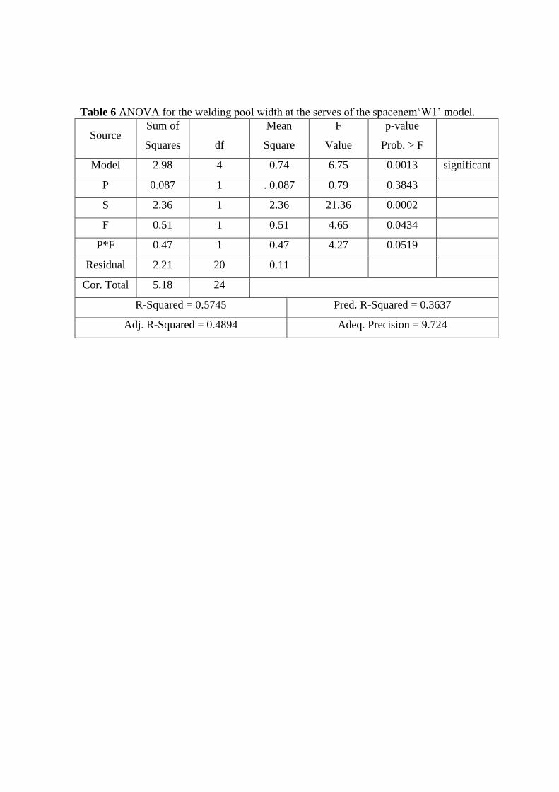
Table 6 ANOVA for the welding pool width at the serves of the spacenem‘W1’ model.

Source Sum of

Squares

df

Mean

Square

F

Value

p-value

Prob. > F

Model 2.98 4 0.74 6.75 0.0013 significant

P 0.087 1 . 0.087 0.79 0.3843

S 2.36 1 2.36 21.36 0.0002

F

0.51 1 0.51 4.65 0.0434

P*F

0.47 1 0.47 4.27 0.0519

Residual 2.21 20 0.11

Cor. Total 5.18 24

R-Squared = 0.5745 Pred. R-Squared = 0.3637

Adj. R-Squared = 0.4894 Adeq. Precision = 9.724

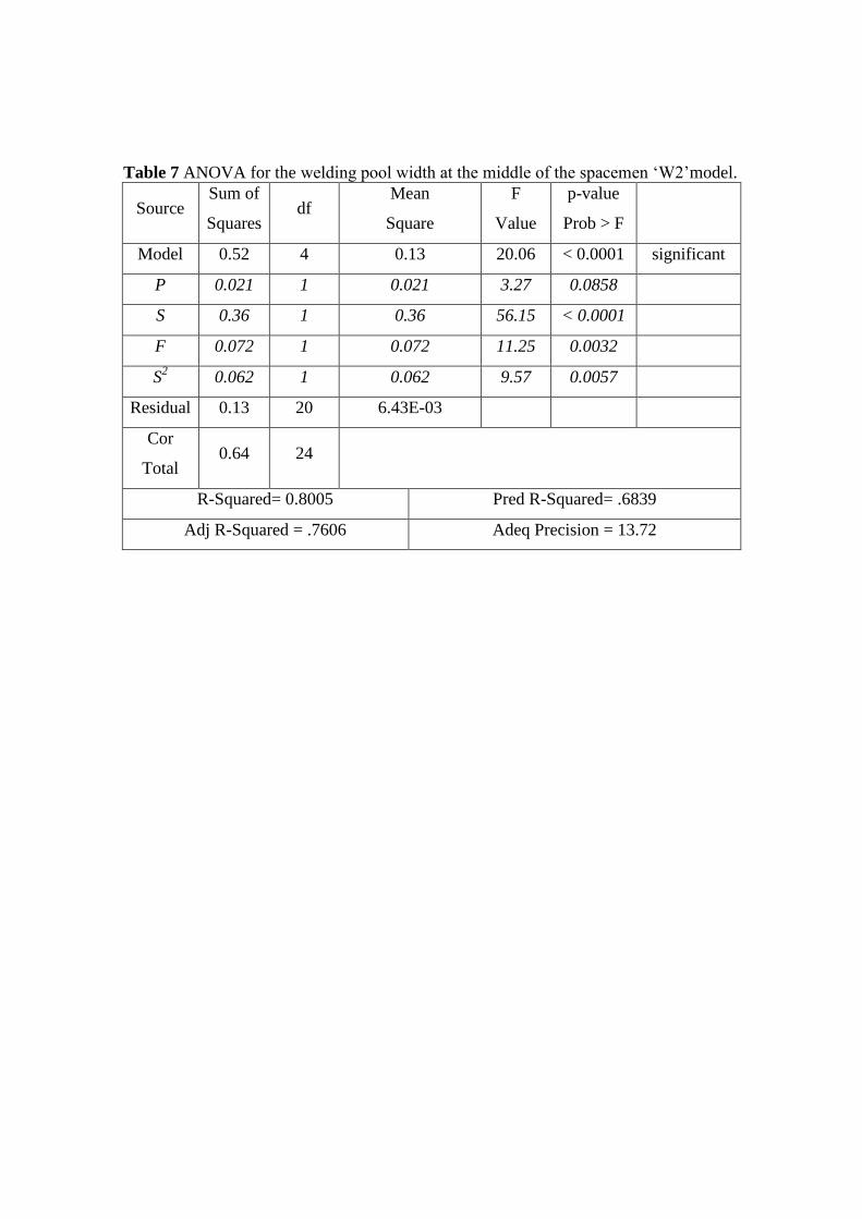
Table 7 ANOVA for the welding pool width at the middle of the spacemen ‘W2’model.

Source Sum of

Squares df

Mean

Square

F

Value

p-value

Prob > F

Model 0.52 4 0.13 20.06 < 0.0001 significant

P 0.021 1 0.021 3.27 0.0858

S 0.36 1 0.36 56.15 < 0.0001

F 0.072 1 0.072 11.25 0.0032

S2 0.062 1 0.062 9.57 0.0057

Residual 0.13 20 6.43E-03

Cor

Total 0.64 24

R-Squared= 0.8005 Pred R-Squared= .6839

Adj R-Squared = .7606 Adeq Precision = 13.72

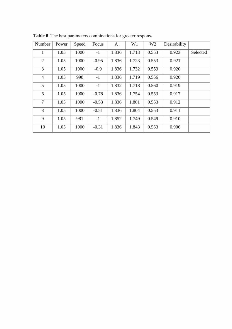
Table 8 The best parameters combinations for greater respons.

Number Power Speed Focus A W1 W2 Desirability

1 1.05 1000 -1 1.836 1.713 0.553 0.923 Selected

2 1.05 1000 -0.95 1.836 1.723 0.553 0.921

3 1.05 1000 -0.9 1.836 1.732 0.553 0.920

4 1.05 998 -1 1.836 1.719 0.556 0.920

5 1.05 1000 -1 1.832 1.718 0.560 0.919

6 1.05 1000 -0.78 1.836 1.754 0.553 0.917

7 1.05 1000 -0.53 1.836 1.801 0.553 0.912

8 1.05 1000 -0.51 1.836 1.804 0.553 0.911

9 1.05 981 -1 1.852 1.749 0.549 0.910

10 1.05 1000 -0.31 1.836 1.843 0.553 0.906

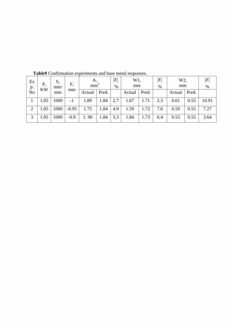
Table9 Confirmation experiments and base metal responses.

Ex

p.

No

P,

KW

S,

mm/

min

F,

mm

A,

mm2

E

%

W1,

mm

E

%

W2,

mm

E

%

Actual Pred. Actual Pred. Actual Pred.

1 1.05 1000 -1 1.89 1.84 2.7 1.67 1.71 2.3 0.61 0.55 10.91

2 1.05 1000 -0.95 1.75 1.84 4.9 1.59 1.72 7.6 0.59 0.55 7.27

3 1.05 1000 -0.9 1. 90 1.84 3.3 1.84 1.73 6.4 0.53 0.55 3.64

Fig. 2, Shows the effect of the welding parameters on the responses (A, W1, W2), and the

variation on weld bead geometry, X10.

X: ActualY: Predicted

Predicted vs. Actual

1.40

1.98

2.55

3.13

3.70

1.50 2.03 2.57 3.11 3.64

Fig. 4, Shows the effect of actual welding parameters on the welding pool area ‘A’

response, against predicted.

X: ActualY: Predicted

Predicted vs. Actual

1.20

1.73

2.25

2.78

3.30

1.21 1.71 2.21 2.71 3.21

Fig. 5, Shows the effect of actual welding parameters on the welding pool width at the

serves of the spacenem‘W1’response, against predicted.

X: ActualY: Predicted

Predicted vs. Actual

0.54

0.68

0.83

0.97

1.11

0.54 0.68 0.82 0.96 1.10

Fig. 6, Shows the effect of actual welding parameters on the welding pool width at the

middle of the spacemen ‘W2’ response, against predicted.

Design-Expert® Software

Fusion Area

Design Points

3.641

1.598

X1 = A: Power

X2 = B: Speed

Actual Factor

C: Focus = -0.50

1.05 1.15 1.24 1.34 1.43

500.00

625.00

750.00

875.00

1000.00Fusion Area

P, kW

S, m

m/m

in

1.745

2.043

2.341

2.638

2.936

Fig. 7, Shows the contour graph of the effect of laser power ‘P’ and welding speed ‘S’

parameters on the welding pool area ‘A’ response, at focus value ‘F’ = -0.5.

Design-Expert® Software

W1

Design Points

3.211

1.213

X1 = A: Power

X2 = C: Focus

Actual Factor

B: Speed = 750.00

1.05 1.15 1.24 1.34 1.43

-1.00

-0.75

-0.50

-0.25

0.00W1

P, kW

F, m

m

1.76119

1.9222

2.0832

2.2442

2.2442

2.40521

Fig. 8, Shows the contour graph of the effect of laser power ‘P’ and focus position ‘F’

parameters on the welding pool width at the serves of the spacenem‘W1’response, at

welding speed ‘S’ = 750mm/min.

Design-Expert® Software

W2

Design Points

1.103

0.544

X1 = A: Power

X2 = B: Speed

Actual Factor

C: Focus = -0.50

1.05 1.15 1.24 1.34 1.43

500.00

625.00

750.00

875.00

1000.00W2

P, kW

S, m

m/m

in

0.686037

0.759143

0.832249

0.905354

0.97846

Fig. 9, Shows the contour graph of the effect of laser power ‘P’ and welding speed ‘S’

parameters on the welding pool width at the middle of the spacemen ‘W2’ response, at

focus value ‘F’ = -0.5 mm.

1.05

1.15

1.24

1.34

1.43 500.00

625.00

750.00

875.00

1000.00

1.400

1.875

2.350

2.825

3.300

F

usi

on

Are

a

P, kW S, mm/min

Fig. 10, Shows 3D graph of the effect of ‘P’ and ‘S’ on welding pool area ‘A’ response, at

‘F’ = −0.5 mm.

500.00

625.00

750.00

875.00

1000.00

-1.00

-0.75

-0.50

-0.25

0.00

1.4

1.875

2.35

2.825

3.3

W

1

S, mm/min

F, mm

Fig. 11, Shows 3D graph of the effect of ‘S’ and ‘F’ on welding pool width at the surface

‘W1’ response, at ‘P’ = 1.24kW.

1.05

1.15

1.24

1.34

1.43

500.00

625.00

750.00

875.00

1000.00

0.61

0.7375

0.865

0.9925

1.12

W

2

P, kW

S, mm/min

Fig. 12, Shows 3D graph of the effect of ‘P’ and ‘S’ on welding pool width at the middle

of the spacemen ‘W2’ response, at ‘F’ = −0.5 mm.

.