Using a DEM to Determine Geospatial Object

Trajectories

Robert T. Collins, Yanghai Tsin,

J. Ryan Miller and Alan J. Lipton

CMU-RI-TR-98-19

The Robotics Institute

Carnegie Mellon University

Pittsburgh, PA 15213

Abstract

This paper addresses the estimation of moving object trajectories within a geospatial coordinate

system, using a network of video sensors. A high-resolution (0.5m grid spacing) digital elevation

map (DEM) has been constructed using a helicopter-based laser range-finder. Object locations are

estimated by intersecting viewing rays from a calibrated sensor platform with the DEM. Contin-

uous object trajectories can then be assembled from sequences of single-frame location estimates

using spatio-temporal filtering and domain knowledge.

c 1998 Carnegie Mellon University

Funded by DARPA contract DAAB07-97-C-J031.The views and conclusions contained in this document are those of the authors and should not be interpreted as

representing the official policies or endorsements, either expressed or implied, of Carnegie Mellon University.

1 Introduction

Carnegie Mellon University and the Sarnoff Corporation are developing a Video Surveillance and

Monitoring (VSAM) testbed that can seamlessly track human and vehicle targets through a large,

visually complex environment. This apparent seamlessness is achieved using a network of active

sensors to cooperatively track targets that cannot be viewed continuously by a single sensor alone.

As targets move out of the active field-of-view of one sensor, they are “handed-off” to another

sensor in the network. Automated target hand-off requires representing the geometric relation-

ships between: 1) multiple sensor locations and their potential fields-of-view, 2) target locations,

velocities, and predicted paths, and 3) locations of scene features that may occlude sensor views

or influence target motion (roads, doorways). In the VSAM testbed, this information is made ex-

plicit by representing all sensor pose information, target trajectories, and site models in a single

geospatial coordinate system.

This paper addresses the issue of estimating geospatial target trajectories. In addition to their

uses in planning sensor hand-off, such trajectories can be used to generate visual activity synopses

for review by a human observer, to perform motion-based inferences about target behavior such

as loitering, and to detect multi-agent interactions such as rendezvous or convoying. In regions

where multiple sensor viewpoints overlap, object trajectories can be determined very accurately

by wide-baseline stereo triangulation. However, regions of the scene that can be simultaneously

viewed by multiple sensors are likely to be a small percentage of the total area of regard in real

outdoor surveillance applications, where it is desirable to maximize coverage of a large area given

finite sensor resources.

Determining target trajectories from a single sensor requires domain constraints, in this case

the assumption that the object is in contact with the terrain. This contact location is estimated

by passing a viewing ray through the bottom of the object in the image and intersecting it with

the a digital elevation map (DEM) representing the terrain. Sequences of location estimates over

time are then assembled into consistent object trajectories. Previous uses of the ray intersection

technique for object localization have been restricted to small areas of planar terrain, where the

relation between image pixels and terrain locations is a simple 2D homography [3, 4, 6]. This

has the benefit that no camera calibration is required to determine the backprojection of an image

point onto the scene plane, provided the mappings of at least 4 coplanar scene points are known

beforehand. However, the VSAM testbed is designed for much larger scene areas that may contain

significantly varied terrain.

The remainder of this paper discusses site modeling issues, emphasizing construction of a

high-resolution DEM using a laser range-finder, the basic ray intersection technique for producing

1

an estimate of object location from a single frame, and finally, techniques for producing consistent

object trajectories from sequences of location estimates. Everything is illustrated using results from

a VSAM testbed demonstration held in November 1997 at CMU’s Bushy Run research facility.

2 Site Modeling

The term “geo”spatial refers to coordinate systems that represent locations on the surface of the

Earth geoid – the ultimateabsoluteframe of reference for planetary activities. This does not

necessarily imply a spherical coordinate system – local coordinate systems such as map projections

can be geospatial if the transformation from local to geodetic coordinates is well documented.

The primary benefit gained by firmly anchoring the VSAM testbed in geospatial coordinates is

the ability to index into off-the-shelf cartographic modeling products. It is envisioned that future

VSAM systems could be rapidly deployed to monitor trouble spots anywhere on the globe, with

an initial site model being quickly generated from archived cartographic products or via aerial

photogrammetry.

2.1 Coordinate Systems

Two geospatial site coordinate systems are used interchangeably within the VSAM testbed. The

WGS84 geodetic coordinate system (“GPS” coordinates) provides a reference frame that is stan-

dard, unambiguous and global (in the true sense of the word). Unfortunately, even simple com-

putations such as the distance between two points become complicated as a function of latitude,

longitude and elevation. For this reason, geometric processing is performed within a site-specific

Local Vertical Coordinate System (LVCS) [1]. An LVCS is a Cartesian system oriented so that

the positive X axis points east, positive Y points true north, and positive Z points up (anti-parallel

to gravity). All that is needed to completely specify an LVCS is the 3D geodetic coordinate of its

origin point. Conversion between geodetic and LVCS coordinates is straightforward, so that each

can be used as appropriate to a task.

For purposes of calibration and ground truth surveying, a GPS base station and rover configu-

ration was established at the Bushy Run site using a pair of Ashtech Z-surveyer receivers. Using

dual-frequency, carrier phase differential correction techniques, this system can measure locations

with a horizontal accuracy of 1 cm (rms) when stationary and to within 3 cm (rms) when on the

move. Vertical position estimates are roughly 1.7 times less accurate (1.7 cm static, 5 cm on the

move).

2

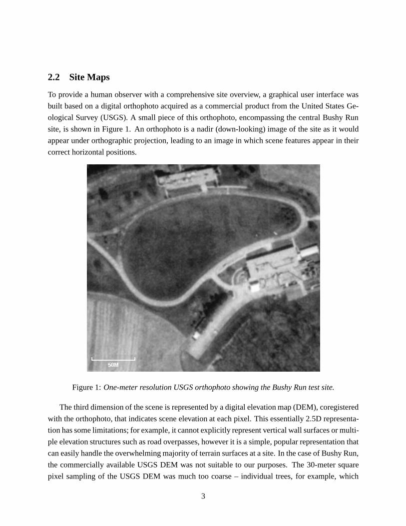
2.2 Site Maps

To provide a human observer with a comprehensive site overview, a graphical user interface was

built based on a digital orthophoto acquired as a commercial product from the United States Ge-

ological Survey (USGS). A small piece of this orthophoto, encompassing the central Bushy Run

site, is shown in Figure 1. An orthophoto is a nadir (down-looking) image of the site as it would

appear under orthographic projection, leading to an image in which scene features appear in their

correct horizontal positions.

Figure 1:One-meter resolution USGS orthophoto showing the Bushy Run test site.

The third dimension of the scene is represented by a digital elevation map (DEM), coregistered

with the orthophoto, that indicates scene elevation at each pixel. This essentially 2.5D representa-

tion has some limitations; for example, it cannot explicitly represent vertical wall surfaces or multi-

ple elevation structures such as road overpasses, however it is a simple, popular representation that

can easily handle the overwhelming majority of terrain surfaces at a site. In the case of Bushy Run,

the commercially available USGS DEM was not suitable to our purposes. The 30-meter square

pixel sampling of the USGS DEM was much too coarse – individual trees, for example, which

3

have a great impact on occlusion analysis, are completely indistinguishable at this resolution. In

addition, USGS DEMs have been edited to explicitly remove building structures, which are useful

for high-level reasoning about human activities. For these reasons, a custom DEM with half-meter

pixel spacing was constructed using a laser range-finder mounted on a robotic helicopter. Since

this high-resolution DEM is crucial to the target geolocation algorithm, the construction process is

described in detail below.

2.3 High-Resolution DEM

The CMU autonomous helicopter project is developing an aerial laser mapping system [2, 9]. The

CMU helicopter is a mid-sized, unmanned helicopter that is capable of fully autonomous takeoff,

flight path tracking, accurate (< 20 cm) stationary hover, and landing. The laser scanning system

is one of the sensor packages that can be flown aboard the helicopter. Ultimately, this scanner

will automatically develop highly accurate (10 cm) 3D models of large environments, in a more

efficient manner than is provided by existing techniques.

2.3.1 Laser Mapping System

Mounted beneath the helicopter is a simple laser scanner that scans the terrain in a plane perpen-

dicular to the helicopter’s direction of forward flight (Figure 2). This scanning motion, combined

with the forward motion of the helicopter, allows patches of terrain up to 200m wide to be mea-

sured in a single pass. Larger areas are scanned by systematically flying patterns that completely

cover the area.

Figure 2:Aerial mapping with a single planar scanner.

4

The scanner uses a Riegl LD-90 time-of-flight laser range-finder to measure the straight line

distance from the scanner to a target point on the terrain. A single motor/encoder combination

positions a mirror to scan the laser’s beam through the scanning plane. The scanning system

requires that the position and attitude of the helicopter be known at all times to correctly determine

the real coordinates of the sampled points. The test system uses a Novatel RT-20 GPS receiver to

measure position, a pair of Gyration gyroscopes to measure pitch and roll, and a KVH flux-gate

compass to measure yaw.

2.3.2 Bushy Run Mapping Procedure

The Bushy Run site was scanned to provide a high resolution DEM for object geolocation. The

procedure for generating the DEM was as follows: 1) A GPS differential correction base station

was setup at the Bushy Run site. 2) The helicopter mapping system was prepared for flight, and a

local navigation frame was selected. 3) The helicopter mapping system was flown to scan the entire

Bushy Run site. During the scan, the helicopter’s position and attitude were collected and sent to

ground computers for storage. Similarly, the laser scanner’s measurements were also stored on the

ground computers. 4) After the flights, the stored helicopter position and attitude were combined

with the laser scanner’s data to compute 3D coordinates of each point sampled by the laser range-

finder. 5) The 3D data points were transformed from the helicopter’s local navigation frame to the

VSAM LVCS frame. 6) A DEM grid with cell size 0.5 m x 0.5 m was initialized. Each 3D point

was assigned to one of the cells of the DEM by simply ignoring its Z component and allowing it

to fall into one of the cells. For each cell of the DEM, three statistics were computed: the mean

elevation of all points landing in that cell, the variance in the elevation of these points, and the total

number of points. These three matrices comprise the resulting DEM.

2.3.3 Bushy Run Results

The Bushy Run site is approximately 300m x 300m, and has an asphalt road surrounding an open

field with two large buildings and trees surrounding the area. A test pilot manually flew the heli-

copter about 10 meters above the road as the system scanned the surrounding environment. The

flight was approximately 5 minutes in duration, and collected over 2.5 million 3D data points.

Figure 3 shows a point cloud visualization of the data. For display purposes, each point is shaded

based on a combination of elevation, and on return intensity of the laser. As such, the road is

readily visible. It should also be noted that since the helicopter was flown above the road, the low

density of measurements from the center of the field is expected.

Figure 4 shows a digital elevation map with 0.5m square grid spacing, generated from the scan

5

Figure 3:Perspective view of 3D point cloud from test scan.

6

data. The intensity of each pixel indicates the average elevation measured for that location. A side-

by-side comparison of this image with the orthophoto in Figure 1 indicates that the mapping system

is producing reasonable results. For purposes of geolocation estimation, holes in the DEM (black

areas in Figure 4) were filled be inserting bilinearly interpolated values from the USGS 30-meter

DEM. This fusion of information was possible since both DEMS are precisely geolocated.

Figure 4:Half-meter resolution DEM showing same area as orthophoto in Figure 1. Intensity has

been enhanced to emphasize terrain variation.

3 Estimating Target Location

The VSAM testbed contains highly effective algorithms for detecting, classifying and tracking

moving targets through a 2D video sequence [7]. Target locations in the scene are estimated from

the bounding box of stable motion regions in each frame of the sequence. Each location estimate

is obtained by shooting a 3D viewing ray through the center of the bottom edge of the target image

7

bounding box out into the scene, and determining where it intersects the terrain. This procedure is

illustrated in Figure 5.

User view

Figure 5:Estimating object locations by intersecting view rays with a terrain model.

3.1 Camera Calibration

Calibration of the internal (lens) and external (pose) sensor parameters is necessary in order to

determine how each pixel in the image relates to a viewing ray in the scene. The internal parameters

of the sensor are determined manually, off-line. The external parameters consist of sensor location

and orientation, measured with respect to the site LVCS. These are determined as part of the sensor

setup procedure. Each sensor is mounted rigidly to a pan-tilt head, which in turn is mounted on a

leveled tripod, thus fixing the roll and tilt angles of the pan-tilt-sensor assembly to be zero. The

location(x0; y0; z0) of the sensor is determined by GPS survey.

8

The only other degree of pose freedom is the yaw angle (horizontal orientation) of the sensor

assembly. This angle is estimated using a set of vertical landmarks distributed around the site,

whose horizontal locations(xi; yi) are known (surveyed by GPS). For each visible landmark the

pan-tilt assembly is guided (by hand) to pan until the landmark is centered in the camera image,

thereby measuring a set of pan anglesfpaniji = 1; :::; ng. Each measured pan angle yields an

independent estimate�i of camera yaw as

�i = atan2(yi � y0; xi � x0) � pani :

A final yaw estimate� is computed as the average of these angles, taking care to use the appropriate

formula for averaging angular data [8], namely

� = atan2(nX

1

sin �i;nX

1

cos �i) :

3.2 Ray Intersection with the DEM

Given a calibrated sensor, and an image pixel corresponding to the assumed contact point between

an object and the terrain, a viewing ray(x0+ku; y0+kv; z0+kw) is constructed, where(x0; y0; z0)

is the 3D sensor location,(u; v; w) is a unit vector designating the direction of the viewing ray

emanating from the sensor, andk � 0 is an arbitrary distance. General methods for determining

where a viewing ray first intersects a 3D scene (for example, ray tracing) can be quite involved.

However, when scene structure is stored as a DEM, a simple geometric traversal algorithm suggests

itself, based on the well-known Bresenham algorithm for drawing digital line segments. Consider

the vertical projection of the viewing ray onto the DEM grid (see Figure 6). Starting at the grid

cell (x0; y0) containing the sensor, each cell(x; y) that the ray passes through is examined in turn,

progressing outward, until the elevation stored in that DEM cell exceeds thez-component of the

3D viewing ray at that location. Thez-component of the view ray at location(x; y) is computed

as either

z0 +(x� x0)

uw or z0 +

(y � y0)

vw (1)

depending on which direction cosine,u or v, is larger. This approach to viewing ray intersection

localizes objects to lie within the boundaries of a single DEM grid cell. A more precise sub-cell

location estimate can then be obtained by interpolation. If multiple intersections with the terrain

beyond the first are required, this algorithm can be used to generate them in order of increasing

distance from the sensor, out to some cut-off distance.

9

Elev( X0+kU, Y0+kV ) > Z0 + kW

11

X0, Y0, Z0

X

01

2

10

8

7

4

6

9

3

5

12

13

Projection

X0, Y0

Ray: (X0,Y0) + k(U,V)

Ray: (X0,Y0,Z0) + k(U,V,W)

Vertical

X

Figure 6: A Bresenham-like traversal algorithm determines which DEM cell contains the first

intersection of a viewing ray and the terrain.

10

4 Assembling Target Trajectories

Computation of dynamic object trajectories in the scene is useful for planning sensor hand-off,

generating visual activity summaries, and for performing qualitative behavior analysis. The pre-

vious section described how target locations can be estimated from each frame by intersecting

viewing rays with a DEM. This section discusses the assembly of single-frame location estimates

into continuous scene trajectories using spatio-temporal filtering and domain knowledge.

4.1 Spatio-Temporal Filtering

Target trajectories can be created by simply concatenating a sequence of static object geolocations.

However, some of these single-frame location estimates may be in error, due to imprecision in the

motion region bounding box. Furthermore, a single viewing ray may intersect the terrain multiple

times, and the first intersection is not always the correct one, since our “terrain” representation also

contains trees and buildings that may occlude parts of the object. An example of this is shown in

Figure 7a, corresponding to a video sequence in which a tracked vehicle became partially occluded

by a tree. Composing single-frame estimates of the first intersection of the target viewing ray with

the terrain generates a scene trajectory that incorrectly appears to swerve into the tree. Figure 7b

shows a better trajectory, generated by taking thelast intersection between the viewing ray and the

terrain. Although this simple heuristic is effective in removing errors caused by occluding foliage,

it may yield incorrect results in rugged or hilly terrain, when multiple elevation structures such as

bridges exist, or in the case of a person walking on a building roof.

A more general mechanism for assembling location estimates into smooth, continuous object

trajectories is spatio-temporal filtering. For example, Kalman filtering could be used to build a

dynamic model of the target, based on the assumption that the target will not make sharp turns and

abrupt accelerations [3, 6]. However, as mentioned above, a viewing ray may intersect the terrain

multiple times, resulting in several alternative hypotheses for target location. The Kalman filter,

based on unimodal Gaussian densities, cannot simultaneously represent these multiple possible

paths, and an incorrect choice of initial value will doom the entire trajectory. What is required is a

more advanced filtering method that can handle multiple data associations, such as the CONDEN-

SATION algorithm [5]. This is a topic of current work.

4.2 Domain Knowledge

Notwithstanding the need for a powerful, general mechanism to generate smooth target trajecto-

ries, in certain cases domain knowledge can be used to generate simpler, approximate solutions. In

11

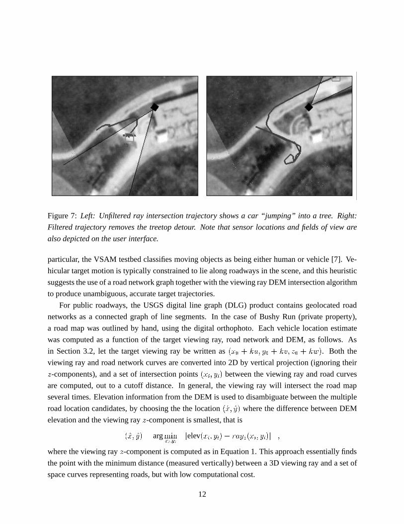
Figure 7: Left: Unfiltered ray intersection trajectory shows a car “jumping” into a tree. Right:

Filtered trajectory removes the treetop detour. Note that sensor locations and fields of view are

also depicted on the user interface.

particular, the VSAM testbed classifies moving objects as being either human or vehicle [7]. Ve-

hicular target motion is typically constrained to lie along roadways in the scene, and this heuristic

suggests the use of a road network graph together with the viewing ray DEM intersection algorithm

to produce unambiguous, accurate target trajectories.

For public roadways, the USGS digital line graph (DLG) product contains geolocated road

networks as a connected graph of line segments. In the case of Bushy Run (private property),

a road map was outlined by hand, using the digital orthophoto. Each vehicle location estimate

was computed as a function of the target viewing ray, road network and DEM, as follows. As

in Section 3.2, let the target viewing ray be written as(x0 + ku; y0 + kv; z0 + kw). Both the

viewing ray and road network curves are converted into 2D by vertical projection (ignoring their

z-components), and a set of intersection points(xi; yi) between the viewing ray and road curves

are computed, out to a cutoff distance. In general, the viewing ray will intersect the road map

several times. Elevation information from the DEM is used to disambiguate between the multiple

road location candidates, by choosing the the location(x; y) where the difference between DEM

elevation and the viewing rayz-component is smallest, that is

(x; y) = argminxi;yi

jelev(xi; yi)� rayz(xi; yi)j ;

where the viewing rayz-component is computed as in Equation 1. This approach essentially finds

the point with the minimum distance (measured vertically) between a 3D viewing ray and a set of

space curves representing roads, but with low computational cost.

12

Figure 8 shows an activity synopsis generated using this approach, in the form of a long-term

vehicle trajectory around the Bushy Run site. Two sensors cooperatively track a vehicle that drives

into the site from the left, descends a hill into a parking lot, stops and turns around, then proceeds

out of the parking lot and continues in its counterclockwise journey around the site. Gaps in the

trajectory correspond to hand-off regions and occlusion areas where neither sensor was reliably

tracking the object.

Figure 8:Activity synopsis of a vehicle driving through Bushy Run.

5 Current Work

This year the VSAM IFD demo will be held in and around the CMU campus, and feature nearly

a dozen sensors tracking objects throughout a cluttered, urban environment. A full geospatial

site model of the area is currently being constructed, including terrain, road networks, sidewalks,

bridges, building volumes, and specific trees. The VSAM testbed will be able to manipulate these

site model elements using libCTDB, a library of geometric utilities for interacting with a geospa-

tial database, developed within the military’s synthetic environments program. LibCTDB will sup-

13

port the VSAM testbed’s need for occlusion analysis and ray intersection to support multi-sensor

hand-off, as well as offer an interface to fully interactive, 3D dynamic visualization packages. Fur-

thermore, more general methods of performing spatio-temporal filtering given multiple competing

location hypotheses are being pursued.

Acknowledgements

We wish to thank Omead Amidi and Marc DeLouis for designing, building and operating the CMU

Robot Helicopter, Daniel Morris for implementing the Bresenham-like ray intersection algorithm,

and the cast and crew of the 1997 VSAM demo.

References

[1] American Society of Photogrammetry,Manual of Photogrammetry,Fourth Edition, Ameri-

can Society of Photogrammetry, Falls Church, VA, 1980.

[2] O.Amidi, T.Kanade and R.Miller, “Vision-based Autonomous Helicopter Research at

Carnegie Mellon Robotics Institute,”Proceedings of Heli Japan ’98,Gifu, Japan, April 1998.

[3] K.Bradshaw, I.Reid and D.Murray, “The Active Recovery of 3D Motion Trajectories and

Their Use in Prediction,”IEEE PAMI,Vol.19(3), March 1997, pp. 219-234.

[4] B.Flinchbaugh and T.Bannon, “Autonomous Scene Monitoring System”, Proc. 10th Annual

Joint Government-Industry Security Technology Symposium, American Defense Prepared-

ness Association, June 1994.

[5] M.Isard and A.Blake, “Contour Tracking by Stochastic Propagation of Conditional Density,”

Proc. ECCV,1996, pp. 343-356.

[6] D.Koller, K.Daniilidis, and H.Nagel, “Model-Based Object Tracking in Monocular Image

Sequences of Road Traffic Scenes,IJCV,Vol.10(3), June 1993, pp. 257-281.

[7] A.Lipton, H.Fujiyoshi, and R.Patil, “Moving Target Identification and Tracking from Real-

time Video,”submitted to WACV 1998.

[8] K.V.Mardia, Statistics of Directional Data,Academic Press, New York, 1972.

[9] R.Miller and O.Amidi, “3-D Site Mapping with the CMU Autonomous Helicopter,” To ap-

pear inProc. 5th Intl. Conf. on Intelligent Autonomous Systems,Sapporo, Japan, June 1998.

14