Statistical Methods In Proteomics

Weichuan Yu1, Baolin Wu5, Tao Huang1,Xiaoye Li2, Kenneth Williams3, Hongyu Zhao1,4

1 Department of Epidemiology and Public Health,2 Department of Applied Mathematics,

3 Keck Laboratory, 4Department of Genetics,Yale University,

New Haven, CT 06520, USA

5Division of Biostatistics, School of Public Health,University of Minnesota,

Minneapolis, MN 55455, USA

December 20, 2004

Summary

Proteomics technologies are rapidly evolving and attracting great attentionin the post-genome era. In this chapter, we review two key applicationsof proteomics techniques: disease biomarker discovery and protein/peptideidentification. For each of the applications, we will state the major issuesrelated to statistical modeling and analysis, review related work, discuss theirstrength and weakness, and point out unsolved problems for future research.

Concretely, we organize this chapter as follows: Section 1 briefly introducesmass spectrometry (MS) and tandem MS/MS with a few sample plots show-ing data format. Section 2 focuses on MS data pre-processing. We first

1

review approaches in peak identification, then address the problem of peakalignment. After that, we point out unsolved problems and propose a fewpossible solutions.

Section 3 addresses the issue of feature selection. We start with a simpleexample showing the effect of large number of features. Then we address theinteraction of different features and discuss methods of reducing the influenceof noise. We finish this section with some discussion on the applicationof machine learning methods in feature selection. Section 4 addresses theproblem of sample classification. We specifically describe the random forestmethod in detail in section 5.

In section 6 we address protein/peptide identification. We first review databasesearching methods in section 6.1, then focus on De Novo MS/MS sequencingin section 6.2. After reviewing major protein/peptide identification programslike SEQUEST and MASCOT in section 6.3, we point out some major issuesthat remain to be addressed in protein/peptide identification to conclude thesection.

Proteomics technologies are considered the major player in the analysis andunderstanding of protein function and biological pathways. Developments ofstatistical methods and software for proteomics data analysis will continueto be the focus in proteomics in the years to come.

Keywoards: proteomics, biomarker discovery, peak identification,peak alignment, feature selection, sample classification, machine learning,random forest, protein/peptide identification.

1 Introduction

In the post-genome era, proteomics has attracted more and more attentiondue to its potential in understanding biological functions and structures atthe protein level. Although recent years have witnessed great advancementin the collection and analysis of gene expression microarray data, proteins

2

are in fact the functional units that are of biological relevance. The oftenpoor correlation that exists between levels of mRNA versus protein expres-sion (Greenbaum et al., 2001), and the rapid advances in mass spectrometry(MS) instrumentation and attendant protein profiling methodologies havesubstantially increased interest in using MS approaches to identify peptideand protein biomarkers of disease. This great level of interest arises fromthe high potential of biomarkers to provide earlier diagnosis, more accurateprognosis and disease classification; to guide treatment; and to increase ourunderstanding at the molecular level of a wide range of human diseases. Thischapter focuses on two key applications of proteomics technologies: diseasebiomarker discovery and protein identification through MS data. We antic-ipate that the statistical methods and computer programs will contributegreatly to the discovery of disease biomarkers as well as the identification ofproteins and their modification sites. These methods should help biomedicalresearchers to better realize the potential contribution of rapidly evolvingand ever more sophisticated MS technologies and platforms.

The study of large-scale biological systems has become possible thanks toemerging high-throughput mass spectrometers. Basically, a mass spectrom-eter consists of three components: ion source, mass analyzer, and detector.The ion source ionizes molecules of interest into charged peptides, the massanalyzer accelerates these peptides with an external magnetic field and/orelectric field, and the detector generates a measurable signal when it detectsthe incident ions. This procedure of producing MS data is illustrated in fig-ure 1. Data resulting from MS sources have a very simple format consistingentirely of paired mass-charge-ratio (m/z value) versus intensity data points.Figure 2 shows a few examples of the raw MALDI-MS data.

The total number of measured data points is extremely large (about 105 fora conventional MALDI-TOF instrument as compared to perhaps 106 for aMALDI-FTICR instrument covering the range from 700−28, 000 Da), whilethe sample size is usually in the magnitude of hundreds. This very high ratioof data size to sample size poses unique statistical challenges in MS dataanalysis. It is desired to find a limited number of potential peptide/proteinbiomarkers from the vast amount of data in order to distinguish cases fromcontrols and enable classification of unknown samples. This process is oftenreferred to as biomarker discovery. In this chapter, we review key steps inbiomarker discovery: pre-processing, feature selection, and sample classifica-tion.

3

Figure 1: The principle of MS data generation: Molecules are ionized intopeptides in ionizer. The peptides are accelerated and separated by analyzerand then detected by detector.

A biomarker discovered in the MS data may correspond to many possiblebiological sources (i.e., a spectral peak may come from different proteins).Therefore, it is necessary to identify peptides and their parent proteins inorder to fully understand the relation between protein structure and diseasedevelopment. This understanding can also be very useful in drug design anddevelopment.

In order to identify proteins in complex mixtures, tandem MS technique(MS/MS), coupled with database searching, has become the method of choicefor the rapid and high-throughput identification, characterization, and quan-tification of proteins. In general, a protein mixture of interest is enzymati-

4

400

600

800

1000

1200

Sam

ple

1

500

1000

1500

2000

2500

3000

Sam

ple

2

2000

4000

6000

8000

Sam

ple

3500

1000

1500

2000

2500

3000

1000 1500 2000 2500 3000S

ampl

e 4

m/z

Figure 2: A few examples of MS raw data. The horizontal axis denotes them/z ratio and the vertical axis denotes the intensity value.

cally digested, and the resulting peptides are then further fragmented throughcollision-induced dissociation (CID). The resulting tandem MS spectrum con-tains information about the constituent amino acids of the peptides andtherefore information about their parent proteins. The process is illustrated

5

in figure 3.

Figure 3: The principle of MS/MS data generation: Peptides are furtherfragmented through collision-induced dissociation (CID) and detected in thetandem MS equipment.

Many MS/MS-based methods have been developed for identifying proteins.The identification of peptides containing mutations and/or modifications,however, is still a challenging problem. Statistical methods need to be devel-oped for improving identification of modified proteins in samples consistingof only a single protein and also in samples consisting of complex proteinmixtures.

We organize the rest of the chapter as follows: Section 2 describes MS datapre-processing methods. Section 3 focuses on feature selection. Section

6

4 reviews general sample classification methodology and Section 5 mainlydescribes the random forest algorithm. Section 6 surveys different algo-rithms/methods for protein/peptide identification, each with its strengthsand weaknesses. It also points out challenges in the future research and pos-sible statistical approaches in solving these challenges. Section 7 summarizesthe chapter.

2 MS Data Pre-processing

When analyzing MS data, only the spectral peaks that result from ioniza-tion of biomolecules such as peptides and proteins are biologically meaningfuland of use in applications. To detect and locate spectral peaks, different datapre-processing methods have been proposed. A commonly used protocol forMS data pre-processing consists of the following steps: spectrum calibra-tion, base-line correction, smoothing, peak identification, intensity normal-ization and peak alignment (e.g. Wagner et al. (2003), Yasui et al. (2003b),Coombes et al. (2003)).

Pre-processing starts with aligning individual spectra. Even with the use ofinternal calibration, the maximum observed intensity for an internal calibrantmay not occur at exactly the same corresponding m/z value in all spectra.This challenge can be addressed by aligning spectra based on the maximumobserved intensity of the internal calibrant. For the sample collected, thedistance between each pair of consecutive m/z ratios is not constant. Instead,the increment in m/z values is approximately a linear function of the m/zvalues. Therefore, a log-transformation of m/z values is needed before anyanalysis is performed so that the scale on the predictor is roughly comparableacross the range of all m/z values. In addition to transformation on the m/zvalues, we also need to log-transform intensities to reduce the dynamic rangeof intensity values. In summary, log-transformations are needed for both m/zvalues and intensities as the first step in MS data analysis. Figure 4 showsan example of MS data before and after the log-transformation.

Chemical and electronic noise produce background fluctuations, and it isimportant to remove these background fluctuations before further analysis.Local smoothing methods have been utilized for baseline subtraction to re-move high frequency noise, which is apparent in MALDI-MS spectra. In

7

1000 1500 2000 2500 3000 35000

500

1000

1500

2000

2500

3000

3500

4000

m/z

inte

nsity

7 7.5 8−2

0

2

4

6

8

10

log(m/z)lo

g of

inte

nsity

Figure 4: Left: Original raw data. Right: MS data after the log-transformation (top). The result of base line correction is also shown (bot-tom).

the analysis of MALDI data, Wu et al. (2003) used a local linear regressionmethod to estimate the background intensity values, and then subtracted thefitted values from the local linear regression result. Baggerly et al. (2003)proposed a semi-monotonic baseline correction method in their analysis ofSELDI data. Liu et al. (2003) computed the convex hull of the spectrum,and subtracted the convex hull from the original spectrum to get the baselinecorrected spectrum. An example of baseline correction is shown in figure 4as well.

Among the above steps, peak identification and alignment are arguably themost important ones. The inclusion of non-peaks in the analysis will un-doubtedly reduce our ability to identify true biomarkers, while peaks iden-tified need to be aligned so that the same peptide should correspond to thesame peak value.

In the following, we give an overview of the existing approaches related topeak detection and peak alignment.

8

2.1 Peak Detection/Finding

Normally, spectral peaks are local maxima in MS data. Most published algo-rithms on peak identification use local intensity values to define peaks, i.e.,peaks are mostly defined with respect to their nearby points. For example,Yasui et al. (2003a, b) defined a peak as the m/z value that has the highestintensity value within its neighborhood, where the neighbors are the pointswithin a certain range from the point of interest. In addition, a peak musthave an intensity value that is higher than the average intensity level of itsbroad neighborhood. Coombes et al. (2003) considered two peak identifica-tion procedures. For simple peak finding, local maxima are first identified.Then, those local maxima that are likely noise are filtered out, and nearbymaxima that likely represent the same peptides are merged. There is a fur-ther step to remove unlikely peak points. In the simultaneous peak detectionand baseline correction, peak detection is first used to obtain a preliminarylist of peaks, and then baseline is calculated by excluding candidate peaks.The two steps are iterated and some peaks are further filtered out if thesignal-to-noise ratio is smaller than a threshold. Similarly, Liu et al. (2003)declared a point in the spectrum to be a peak if the intensity is a local maxi-mum, its absolute value is larger than a threshold, and the intensity is largerthan a threshold times the average intensity in the window surrounding thispoint.

All these methods are based on similar intuitions and heuristics. Severalparameters need to be specified beforehand in these algorithms, e.g. thenumber of neighboring points and the intensity threshold value. In fact, theparameter settings in the above algorithms are related to our understand-ing/modeling of the underlying noise. To address this issue, Coombes et al.(2003) defined noise as the median absolute value of intensity. Satten et al.(2004) used the negative part of the normalized MS data to estimate the vari-ance of noise. Wavelets based approaches (Coombes et al. (2004), Randolphand Yasui (2004)) have also been proposed to de-noise the MS data beforepeak detection. Based on the observation that there are substantial measure-ment errors in the measured intensities, Yasui and colleagues (2003a) arguedthat binary peak/non-peak data is more useful than the absolute values ofintensity, while they still used a local maximum search method to detectpeaks. Clearly, the success of noise-estimation-plus-threshold methodologylargely depends on the correctness of the noise model, which remains to be

9

validated.

Another issue in peak detection is to avoid false positive detections. This isoften done by adding an additional constraint (e.g. the peak width constraint(Yasui et al. (2003a))) or by choosing a specific scale level after wavelets de-composition of the original MS data (Randolph and Yasui (2004)). In thecase of high resolution data, it has been proposed that more than one iso-topic variant of a peptide peak should be present before a spectral peak isconsidered to result from peptide ionization (Yu et al. (2004)). It may alsobe possible to use prior information about the approximate expected peakintensity distribution of different isotopes arising from the same peptide dur-ing peak detection (i.e., the theoretical relative abundance of the first peptideisotope peak may range from 60.1% for polyGly (n=23, MW 1329.5 Da) to90.2% for poly Trp (n=7, MW 1320.5 Da)(personal communication 11/1/04from Dr. Walter McMurray, Keck Laboratory)). Certainly we also have toconsider the issue of limited resolution and the consequent overlapping effectof neighboring peaks.

2.2 Peak Alignment

After peaks have been detected, we have to align them together before com-paring peaks in different data sets. Previous studies have shown that thevariation of peak locations in different data sets is non-linear (Torgrip etal. (2003), Eilers (2004)). The example in Yu et al. (2004) shows thatthis variation still exists even when we use technical replicates. The reasonsthat underlie data variation are extremely complicated, including differencesin sample preparation, chemical noise, co-crystallization and deposition ofthe matrix-sample onto the MALDI-MS target, laser position on the target,and other factors. Although it is of interest to identify these reasons, weare more interested in finding a framework to reduce the variation and alignthese peaks together.

Towards this direction, some methods have been proposed. Coombes et al.(2003) pooled the list of detected peaks that differed in location by 3 clockticks or by 0.05% of the mass. Yasui et al. (2003a) believed that the m/z axisshift of peaks is approximately ±0.1% to ±0.2% of the m/z value. Thus, theyexpanded each peak to its local neighborhood with the width equal to 0.4%of the m/z value of the middle point. This method certainly oversimplifies

10

the problem. In another study (Yasui et al. (2003b)), they first calculatedthe number of peaks in all samples allowing certain shifts, and selected m/zvalues with the largest number of peaks. This set of peaks is then removedfrom all spectra and the procedure is iterated until all peaks are exhaustedfrom all the samples. In a similar spirit, Tibshirani et al. (2004) proposed touse complete linkage hierarchical clustering in one dimension to cluster peaksand the resulting dendrogram is cut off at a given height. All the peaks inthe same cluster are considered as the same peak in further analysis.

Randolph and Yasui (2004) used wavelets to represent the MS data in a multi-scale framework. They used a coarse-to-fine method to first align peaks ata dominant scale and then refine the alignment of other peaks at a finerscale. From the signal representation point of view, this approach is veryinteresting. But it remains to be determined if the multi-scale representationis biologically reasonable.

Johnson et al. (2003) assumed that the peak variation is less than the typicaldistance between peaks and they used a closest point matching method forpeak alignment. The same idea was also used in Yu et al. (2004) to addressthe alignment of multiple peak sets. Certainly, this method is limited by thedata quality and it cannot handle large peak variation.

Dynamic programming (DP) based approaches (Nielsen et al. (1998), Tor-grip et al. (2003)) have also been proposed. DP has been used in geneexpression analysis to warp one gene expression time series to another sim-ilar series obtained from a different biological replicate (Aach and Church(2001)), where the correspondence between the two gene expression timeseries is guaranteed. In MS data analysis, however, the situation is morecomplicated since a one-to-one correspondence between two data sets doesnot always exist. Although it is still possible to apply DP to deal with theshort-of-correspondence problem, some modifications are necessary (such asadding an additional distance penalty term in the estimation of correspon-dence matrix). It also remains unclear how DP can identify and ignoreoutliers during the matching.

Eilers (2004) proposed a parametric warping model with polynomial func-tions or spline functions to align chromatograms. In order to fix warpingparameters, he added calibration example sequences into chromatograms.While the idea of using parametric model is interesting, it is difficult to re-peat the same parameter estimation method in MS data since we cannot

11

add many calibrator compounds into the MS samples. Also, it is unclear if apolynomial with the second order would be enough to describe the non-linearshift of MS peaks.

Although all these methods are ad hoc, the relatively small number of peaks(compared to the number of collected points) and the relatively small shiftsfrom spectrum to spectrum ensures that these heuristic peak alignmentsshould work reasonably well in practice.

2.3 Remaining Problems and Proposed Solutions

Current peak detection methods (e.g. the local maximum search plus thresh-old method) export detection results simply as peaks or non-peaks. Giventhe noisy nature of MS data, this simplification is prone to the influence ofnoise (noise may also produce some local maximal values) and is very sen-sitive to specific parameter settings (e.g. the intensity threshold value). Inaddition, a uniform threshold value may exclude some weak peaks in the MSdata, while the existence/non-existence of some weak peaks may be the mostinformative biomarkers.

Instead of using a binary output, it would be better to use both peak widthand intensity information as quantitative measures of how likely a candidateis a true peak. We can use a distribution model to describe the typical peakwidth and intensity. The parameters of the distribution can be estimatedusing training samples. Then a likelihood ratio test can be used to replacethe binary peak detection result (either as peak (one) or as non-peak (zero))with a real value. This new measure should provide richer information aboutpeaks. We believe this will help us to better align multiple peak sets.

The challenge in peak alignment is that current methods may not work if wehave large peak variation (like with LC/MS (Liquid Chromatography/MassSpectrometry) data). Another unsolved problem is that it may not be validto assume that the distribution of peaks is not corrupted by noise (i.e., falsepositive detection).

To address these problems, we may consider the “true” locations of peaks asrandom variables and regard the peak detection results as sampling observa-tions. Then, the problem of aligning multiple peak sets is converted to theproblem of finding the mean (or median) values of random variables since

12

we can assume that the majority of peaks should locate close to the “true”locations with only some outliers that do not obey this assumption. Afterthe mean/median values have been found/estimated, the remaining task isto simply align peaks w.r.t. the mean/median standard. Intuitively, the rel-ative distance between a peak and its mean/median standard may be furtherused as a confidence measure in alignment.

3 Feature Selection

For current large-scale genomic and proteomic datasets, there are usuallyhundreds of thousands of features (also called variables exchangeably in thefollowing discussion) but limited sample size, which poses a unique challengefor statistical analysis. Feature selection serves two purposes in this context:for biological interpretation and for reducing the impact of noise.

Suppose we have n1 samples from one group (e.g. cancer patients) and n0

samples from another group (e.g. normal subjects). We have m variables(X1, . . . , Xm) (e.g. m/z ratios). For the k-th variable, the observations are

X1k = (xk1, . . . , xkn1

)

for the first group and

X0k =

(

xk(n1+1), . . . , xk(n1+n0)

)

for the second group. They can be summarized in a data matrix, X = (xij).Assume X1

k are n1 i.i.d. samples from one distribution fk1(x) and X0k are n0

i.i.d. samples from another distribution fk0(x).

Two sample T-test statistic or variants thereof are often used to quantify thedifference between two groups in the analysis of gene expression data (Dudoitet al. (2002b), Tusher et al. (2001), Cui and Churchill (2003))

Ti =xi1 − xi0

√

1n1

σ2i1 + 1

n0

σ2i0

, (1)

where

xi1 =n1∑

k=1

xik, xi0 =n1+n0∑

k=n1+1

xik,

13

σ2i1 =

1

n1 − 1

n1∑

k=1

(xik − xi1)2, σ2

i0 =1

n0 − 1

n1+n0∑

k=n1+1

(xik − xi0)2.

Ti can be interpreted as the standardized difference between these two groups.It is expected that the larger the standardized difference, the more separatedthe two groups are. One potential problem of using t-statistics is its robust-ness, the lack of robustness may be a serious drawback when hundreds ofthousands of features are being screened to identify informative ones.

3.1 A Simple Example for the Effect of Large Numbers

of Features

Although there are hundreds of thousands of peaks representing peptides, weexpect the number of peaks that are informative for disease classification tobe limited. This, coupled with the limited number of samples available foranalysis, poses great statistical challenges for the identification of informativepeaks. Consider the following simple example: suppose n1 = 10, n2 = 10,m0 = 103 peptides showing no difference, and m1 = 40 peptides with dif-ference between the two groups with λ = µ/σ = 1.0. We can numericallycalculate the expected number of significant features for these two groups

N0 = 2m0{1 − T (x, df = 18)},

N1 = m1{T (−x, df = 18, λ = 1.0) + 1 − T (x, df = 18, λ = 1.0)},

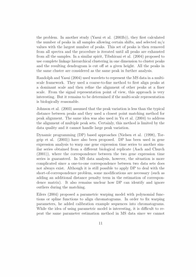
where T (,df) is the t-distribution function with df degrees of freedom, T (,df, λ)is the t-distribution function with df degrees of freedom and non-central pa-rameter λ, and the significance cut-off values are chosen as |T | > x. Figure 5displays the comparison of true and false positives for this example, wherethe diagonal line is also shown. We can clearly see the dominant effect ofnoise in this example.

This artificial example reveals the difficulty of extracting useful featuresamong a large number of noisy features. In practice, due to the noisy na-ture of MS data, the variance σ for individual peptide intensity will be verylarge, reflecting the difficulty of reproducibility, which has been commonlyobserved for MS data. Also, the number of noisy features m0 (mostly un-informative) is increasing exponentially with the advance of technology (e.g.

14

5 10 15 20

050

100

150

N1

N0

Figure 5: Comparison of true positive and false positive for the simulationexample. N1 is the number of true positive, N0 false positive. The diagonalline is also plotted as a solid line. Different points correspond to differentsettings of critical values in the t-test.

MALDI-FTICR data). The combination of these two factors will increasethe ratio of false/true positives.

In this simple example, we ignore the interaction of different prpteins. Forcomplex diseases, e.g. cancer, it is quite possible that the effects result fromthe joint synergy of multiple proteins, while they individually show non-significant differences. Novel statistical methods are needed to account forthe effects of noise and interactions among features.

15

3.2 Interaction

In ordinary or logistic regression models, we describe the interaction of dif-ferent variables by including the interaction terms. This approach quicklybecomes unfeasible with an increasing number of variables. Therefore, stan-dard regression models are not appropriate due to n ≪ p.

Instead of using univariate feature selection methods, it may be useful toconsider multivariate feature selection methods. Lai et al. (2004) analyzedthe co-expression pattern of different genes using a prostate cancer microar-ray dataset, where the goal is to select genes that have differential gene-geneco-expression patterns with a target gene. Some interesting genes have beenfound to be significant and reported to be associated with prostate canceryet none of them showed marginal significant differential gene expressions.

Generally, the multivariate feature selection is a combinatorial approach. Toanalyze two genes at a time we need to consider n2 possibilities instead of nfor the univariate feature selection. For analyzing the interaction of K geneswe need to consider nK possibilities, this quickly becomes intractable.

A Classification and Regression Tree (CART) (Breiman et al. (1984)) natu-rally models the interaction among different variables, and it has been suc-cessfully applied to genomic and proteomic datasets where n ≪ p is to beexpected (e.g. Gunther et al. (2003)).

There are several new developments which are generalizations of the treemodel. Bagging stands for bootstrap aggregating. Intuitively, bagging usesbootstrap to produce pseudo-replicates to improve prediction accuracy (Breiman(1996)). The boosting method (Freund and Schapire (1995)) is a sequentialvoting method, which adaptively re-samples the original data so that theweights are increased for those most frequently misclassified samples. Aboosting model using a tree as the underlying classifier has been successfullyapplied to genomic and proteomic datasets (Adam et al. (2002), Dettlingand Buhlmann (2003)).

3.3 Reducing the Influence of Noise

For most statistical models, the large number of variables may cause an over-fitting problem. Just by chance, we may find some combinations of noise

16

which can potentially discriminate samples with different disease status. Wecan incorporate some additional information into our analysis. For MS data,for instance, we only want to focus on peaks resulting from peptide/proteinionization. In previous sections we have addressed and emphasized the im-portance of MS data preprocessing.

3.4 Feature Selection with Machine Learning Methods

Isabelle et al. (2002) have reported using SVM to select genes for cancerclassification from microarray data. Qu et al. (2002) applied a boostingtree algorithm to classify prostate cancer samples and to select importantpeptides using MS analysis of sera. Wu et al. (2003) reported using randomforest to select important biomarkers from an ovarian cancer data based onMALDI-MS analysis of patient sera.

One distinct property of these learning based feature selection methods com-pared to traditional statistical methods is the coupling of feature selectionand sample classification. They implicitly approach the feature selectionproblem from a multivariate perspective. The significance of a feature highlydepends on other features. In contrast, the feature selection methods em-ployed in Dudoit et al. (2002) and Golub et al. (1999) are univariate andinteractions among genes are ignored.

4 Sample Classification

There are many well established discriminant methods, e.g. linear and quadraticdiscriminant analysis, and k-nearest neighbor, which have been compared inthe context of classifying samples using micorarray and MS data (Dudoit etal. (2002), Wu et al. (2003)). The majority of these methods were devel-oped in the pre-genome era, where the sample size n was usually very largewhile the number of features p was very small. Therefore, directly applyingthese methods to genomic and proteomic datasets does not work. Instead,feature selection methods are usually applied to select some “useful” featuresat first and then the selected features are used to carry out sample classifi-cation based on traditional discriminant methods. This two-step approachessentially divides the problem into two separate steps: feature selection and

17

sample classification, unlike the recently developed machine learning meth-ods where the two parts are combined together.

The previously mentioned bagging (Breiman (1996)), boosting (Freund andSchapire (1997)), random forest (Breiman (2001)), and support vector ma-chine (Vapnik (1998)) approaches have all been successfully applied to high-dimension genomic and proteomic datasets.

Due to the lack of a genuine testing dataset, cross validation (CV) has beenwidely used to estimate the error rate for the classification methods. Inap-propriate use of CV may seriously under-estimate the real classification errorrate. Ambroise and McLachlan (2002) discussed the appropriate use of CVto estimate classification error rate, and recommended the use of K-fold crossvalidation, e.g. K = 5 or 10.

5 Random Forest: Joint Modelling of Fea-

ture Selection and Classification

Wu et al. (2003) compared the performance of several classical discrimi-nant methods and some redently developed machine learning methods foranalyzing an ovarian cancer MS dataset. In this study, random forest wasshown to have good performance in terms of feature selection and sampleclassification. Here we design an algorithm to get an unbiased estimation ofthe classification error using random forest and at the same time efficientlyextract useful features.

Suppose the preprocessed MS dataset has n samples and p peptides. Weuse {Xk ∈ Rp, k = 1, 2, · · · , n} to represent the intensity profile of the k-thindividual, and {Yk, k = 1, 2, · · · , n} to code the sample status.

The general idea of random forest is to combine random feature selectionand bootstrap re-sampling to improve sample classification. We can brieflysummarize the general idea as the following algorithm.

General random forest algorithm

(1) Specify the number of bootstrap samples B, say 105.

18

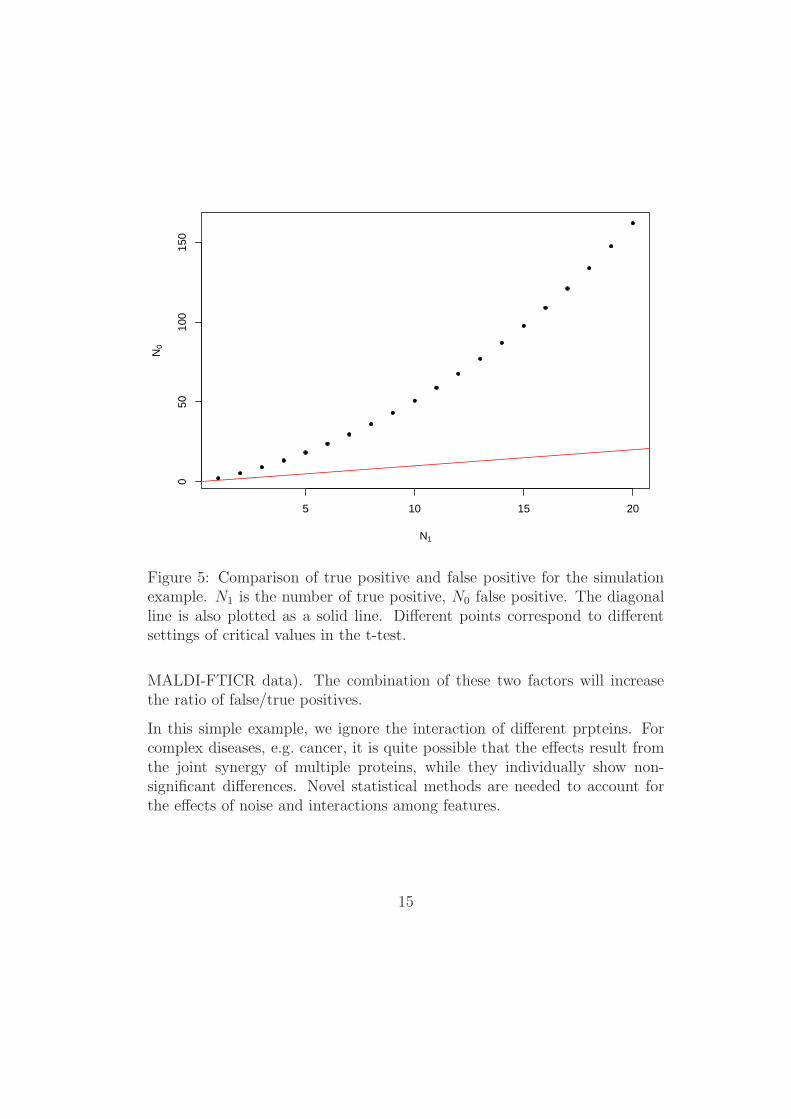
(2) For b = 1, 2, · · · , B,

(2.1) Sample with replacement n samples from {Xk} and denote thebootstrap samples by Xb = {Xb1 , · · · , Xbn

}, the correspondingresponse being Yb = {Yb1, · · · , Ybn

}.

(2.2) Randomly select m out of p peptides. Denote the selected subsetof features by {r1, · · · , rm}, and the bootstrap samples restrictedto this subset by Xb

m. Build a tree classifier Tb using Yb and Xbm.

Predict those samples not in the boostrap samples using Tb.

(3) Average the prediction over bootstrap samples to produce the finalclassification.

For the random forest algorithm from Breiman (2001), randomness is intro-duced at each node split. Specifically, at each node split, a fixed number offeatures is randomly selected from all the features and the best split is cho-sen among these selected features. While for the random subspace methoddeveloped by Ho (1998), a fixed number of features is selected at first andis used for the same original data to produce a tree classifier. Thus, bothmodels have the effect of randomly using a fixed subset of features to producea classifier, but differ in the underlying tree-building method.

Figure 6 shows a simple comparison of the two methods. We selected 78 pep-tides from the ovarian cancer MS data reported at Wu et al. (2003). Then weapply the two algorithms to numerically evaluate their sample classificationperformance using the selected subset of features. We want to emphasizethat the calculated classification error rate is not a true error rate becausewe have used the sample status to select 78 peptides first. Our purpose hereis just to show a simple numerical comparison of these two methods.

Other important issues in the analysis of MS data include specification of thenumber of biomarkers and the sample size incorporated into the experimentaldesign. For estimating classification error Err, as discussed in Cortes et al.(1994), the inverse-power-law learning curve relationship between Err andsample size N ,

Err(N) = β0N−α + β1, (2)

is approximately true for large sample size datasets (usually about tens ofthousands of samples). β1 is the asymptotic classification error and (α, β0)are positive constants.

19

0 200 400 600 800 1000

0.2

0.5

0.8

0 200 400 600 800 1000

0.2

0.5

0.8

Control

Cancer

Error Rate by Random Forest Methoder

ror

rate

0 200 400 600 800 1000

0.2

0.5

0.8

0 200 400 600 800 1000

0.2

0.5

0.8

Control

Cancel

Error Rate by Random Subspace Method

number of trees

erro

r ra

te

Figure 6: Comparison of the error rates of two random forest algorithms onan ovarian cancer data set. 78 features selected by t-test are used in bothalgorithms. The two methods have similar performance.

Current MS data usually have a relatively small sample size (N ∼ 102) com-pared to the high-dimension feature space (p ∼ 105). Under this situation,it may not be appropriate to rely on the learning curve model to extrapolateβ1, which corresponds to an infinite training sample size N = ∞. But withina limited range, this model may be useful to extrapolate the classificationerror. To estimate parameters (α, β0, β1), we need to obtain at least threeobservations.

Obviously the classification error Err also depends on the selected numberof biomarkers m. We are going to use the inverse-power-law (2) to modelErr(N, m).

20

We proposed the following algorithm to get an unbiased estimation for theclassification error rate, which also provides an empirical method to selectthe number of biomarkers (Wu et al. (2004)).

CV error estimation using random forest algorithm

(1) Specify the number of folders K, say 5, and the range for the numberof biomarkers m, say M = {20, 21, · · · , 100}. Randomly divide all Nsamples into balanced K groups.

(2) For k = 1, 2, · · · , K do the following

(2.1) Use samples in the k-th group as the testing set Ts and all theother samples as the training set Tr.

(2.2) Apply the random forest algorithm (or any other feature selectionmethod) to the training data Tr. Rank all the features accordingto their importance.

(2.3) Use the first m ∈ M most important features and construct aclassifier based on the training set Tr and predict samples in thetesting set Ts. We will get a series of error estimates

{

ǫ(

k, m,K − 1

KN

)

, m ∈ M}

,

where K−1K

N is the effective size of the training set.

(2.4) Use samples in the i-th and j-th group as the testing set and otherK − 2 groups as the training set. Repeat step (2.2) and (2.3) toget error estimation

{

ǫ(

k, m,K − 2

KN

)

, m ∈ M}

,

where K−2K

N is the effective size of the training set.

(2.5) We can repeat step (2.4) using n of the groups as testing set andget error rate

{

ǫ(

k, m,K − n

KN

)

, m ∈ M}

, n = 1, 2, · · · , K − 1.

21

(3) Average ǫ(k, m, N(K − n)/K) over K folders to get the final errorestimation ǫ(m, N(K−n)/K) for m biomarkers and sample size N(K−n)/K.

(4) Fit the inverse-power-law model (2) to ǫ(m, N(K − n)/K) for everyfixed m and extrapolate the error rate to N samples, ǫ(m, N).

The estimated error rate curve ǫ(m, n) can be used as a guidance for samplesize calculation and the selection of the number of biomarkers.

20 40 60 80 100

0.15

0.25

0.35

0.45

number of biomarkers

Cla

ssifi

catio

n E

rror

N = 34N = 68N = 102N = 136N = 170

Figure 7: Five-fold cross validation estimation of classification error rateapplying random forest algorithm to the ovarian dataset. The error rates forsample size N = 34, 68, 102, 136 are got from the five-fold CV and the errorrate for N = 170 is extrapolated from the inverse-power-law model fitting.

For K folders, the previous algorithm will involve a total of 2K training setfittings. If K is relatively large, say 10, the total number of fitting will be

22

very large (2K = 1024). Note that in the inverse-power-law model (2) weonly have three parameters (α, β0, β1). We can carry out just enough trainingdata fitting, say 10, to estimate these three parameters. Then we can usethe fitted model to interpolate or extrapolate the classification error rate forother sample size.

Figure 7 displays the 5-fold CV estimation of classification error rate applyingthe random forest algorithm to the serum mass spectrometry dataset for 170ovarian cancer patients reported in Wu et al. (2003), where the error rates forthe training sample size N = 34, 68, 102, 136 are derived from the 5-fold CVand the error rate for N = 170 is extrapolated from the inverse-power-lawmodel fitting.

5.1 Remaining Problems in Feature Selection and Sam-ple Classification

As we discussed before, the univariate feature selection based on t-statisticsis very sensitive to noise. We can reduce the influence of noise marginallyby using additional biological information. But more importantly, we needto develop robust statistical methods. It is conjectured that random forest(Breiman 2001) does not over-fit. Our experience shows that we can dramat-ically reduce the classification error rate by incorporating feature selectionwith the random forest algorithm.

Intuitively, the sample classification error rate will increase with too muchnoise in the data. In this sense, feature selection will help us to improvethe performance of classification algorithms. However, feature selection isusually affected by the small sample size (n ≪ p) in genomic and proteomicdatasets. If we only select a small number of features, we may miss many“useful” features. One approach would be to couple the fast univariate fea-ture selection with the computing-intensive machine learning methods. Forexample, we can first use univariate feature selection to reduce the numberof features to a manageable size M0. Then, we can apply the machine learn-ing methods to refine our selection to a small number of target features M1.Certainly, determining M0 is a trade-off issue: If M0 is too small, we willmiss many informative features; if M0 is too large, we will have a heavy com-puting burden for the following machine learning methods and also make the

23

feature selection unstable.

For the genomic and proteomic data, the large n and small p will makemajority of the traditional statistical methods unusable. Most of the recentlydeveloped machine learning methods are computing-intensive and are oftenevaluated by empirical performance on some datasets. Statistical methodsneeded to be developed to bridge the traditional model-based principle andthe newly developed machine learning methods.

6 Protein/Peptide Identification

6.1 Database Searching

MS in combination with database searching has emerged as a key platform inproteomics for high-throughput identification and quantification of proteins.A single stage MS provides a “mass fingerprint” of the peptide products of theenzymatically digested proteins and can be used to identify proteins (Henzelet al. (1993); James et al. (1993); Mann et al. (1993); Pappin et al. (1993);Yates et al. (1993); Perkins et al. (1999); Clauser et al. (1999); Zhang andChait (2000)). This approach is useful for identifying purified proteins (e.g.proteins in dye-stained spots from 2D polyacrylamide gels) and may alsosucceed with simple mixtures containing only 2-3 major proteins. Proteinidentification based on peptide mass database searching requires high massaccuracy and that observed peptide masses be matched to a sufficient frac-tion (e.g. > 25%) of the putatively identified protein. The latter task will bemade more difficult if the protein has been post-translationally modified atmultiple sites. Alternatively, the resulting peptide ions from the first stageMS can be isolated in the mass spectrometer and individually fragmentedthrough CID to produce a tandem MS. In addition to the parent peptidemass, tandem MS provides structural information that can be used to de-duce the amino acid sequences of individual peptides. Since tandem MS oftenidentifies proteins by using the CID-induced spectrum obtained from a sin-gle peptide, this technology is capable of identifying proteins in very complexmixtures such as cell extracts (Eng et al. (1994), Mann and Wilm (1994),Perkins et al. (1997), Clauser et al. (1999), Pevzner et al. (2000), Bafnaand Edwards (2001), Hansen et al. (2001), Creasy and Cottrell (2002), Field

24

et al. (2002), Keller et al. (2002), MacCoss et al. (2002), Anderson et al.(2003), Colinge et al. (2003), Gasteiger et al. (2003), Havilio et al. (2003),Hernadez et al. (2003), Lu and Chen (2003), Nesvizhskii et al. (2003)). Ingeneral, database searching methods compare the experimentally observedtandem MS with features predicted for hypothetical spectra from candidatepeptides (of equal mass) in the database and then returns a ranked listing ofthe best matches, assuming that the query peptide exists in the protein se-quence database. The statistical challenge in MS and MS/MS-based proteinidentification is to assess the probability that a putative protein identifica-tion is indeed correct. In the case of MS/MS-based approaches, a commonlyused criterion is that the observed MS/MS spectra must be matched to atleast two different peptides from each identified protein.

6.2 De Novo Sequencing

An alternative approach to database searching of uninterpreted tandem MSfor peptide identification is de novo MS/MS sequencing (Taylor and John-son (1997), Dancik et al. (1999), Chen et al. (2001), Ma et al. (2003)),which attempts to derive a peptide sequence directly from tandem MS data.Although de novo MS/MS sequencing can handle situations where a targetsequence is not in the searching protein database, the utility of this approachis highly dependent upon the quality of tandem MS data, such as the num-ber of predicted fragment ion peaks that are observed and the level of noise,as well as the high level of expertise of the mass spectroscopist interpretingthe data as there is no currently accepted algorithm capable of interpretingMS/MS spectra in terms of a de novo peptide sequence without human in-tervention. Because of the availability of DNA sequence databases, manyof which are genome level, and the very large numbers of MS/MS spectra(e.g., tens of thousands) generated in a single isotope coded affinity tag orother MS-based protein profiling analysis of a control versus experimentalcell extract, highly automated database searching of uninterpreted MS/MSspectra is by necessity the current method of choice for high throughputprotein identification (Eng et al. (1994), Perkins et al. (1999), Bafna andEdwards (2001)).

25

6.3 Statistical and Computational Methods

Due to the large number of available methods/alogrithms for MS and MS/MS-based protein identification, we focus on what we believe are currently themost widely used approaches in the field.

• SEQUEST (Eng et al. (1994))

SEQUEST is one of the foremost yet sophisticated algorithms developedfor identifying proteins from tandem MS data. The analysis strategy canbe divided into four major steps: data reduction, search potential peptidematches, scoring peptide candidates and cross-correlation validation. Morespecifically, it begins with computer reduction of the experimental tandemMS data and only retains the most abundant ions to eliminate noise and toincrease computational speed. It then chooses a protein database to searchfor all possible contiguous sequences of amino acids that match the mass ofthe peptide with a predetermined mass tolerance. Limited structure modifi-cations may be taken into account as well as the specificity of the proteolyticenzyme used to generate the peptides. After that, SEQUEST compares thepredicted fragment ions from each of the peptide sequences retrieved from thedatabase with the observed fragment ions and assigns a score to the retrievedpeptide by using several criteria such as the number of matching ions andtheir corresponding intensities, some immoniun ions, and the total numberof predicted sequence ions. The top 500 best fit sequences are then subjectedto a correlation-based analysis to generate a final score and ranking of thesequences.

SEQUEST correlates MS spectra predicted for peptide sequences in a pro-tein database with an observed MS/MS spectrum. The cross-correlationscore function provides a measure of similarity between the predicted andobserved fragment ions and a ranked order of relative closeness of fit of pre-dicted fragment ions from other isobaric sequences in the database. However,since the cross-correlation score does not have probabilistic significance, it isnot possible to determine the probability that the top-ranked and/or othermatches result from random events and are thus false-positives. Althoughlacking a statistical basis, Eng et al. (1994) suggest that a difference greaterthan 0.1 between the normalized cross-correlation functions of the first- andsecond-ranked peptides indicates a successful match between the top-rankedpeptide sequence and the observed spectrum. A commonly used guideline

26

for Sequest-based protein identification is that observed MS/MS spectra arematched to two or more predicted peptides from the same protein and thateach matched peptide meets the 0.1 difference criterion.

• MASCOT (Perkins et al. (1999))

MASCOT is another commonly used database searching algorithm, whichincorporates a probability-based scoring scheme. The basic approach is tocalculate the probability (via an approach that is not well described in theliterature) that a match between the experimental MS/MS data set andeach sequence database entry is a chance event. The match with the lowestprobability of resulting from a chance event is reported as the best match.MASCOT considers many key factors, such as the number of missed cleav-ages, both quantitative and non-quantitative modifications (the number ofnon-quantitative modifications is limited to four), mass accuracy, the par-ticular ion series to be searched and peak intensities. Hence, MASCOTiteratively searches for the set of the most intense ion peaks which providethe highest score - with the latter being reported as −10 log(P ) where P isthe probability of the match resulting from a random, chance event. Perkinset al. (1999) suggested that the validity of the MASCOT probabilities betested by repeating the search against a randomized sequence database andby comparing the MASCOT results with those obtained via the use of othersearch engines.

• Other Methods

In addition to SEQUEST and MASCOT, many other methods have beenproposed to identify peptides and proteins from tandem MS data. They rangefrom the development of probability-based scoring schemes, the identificationof modified peptides, the validation of peptide and protein identifications toother miscellaneous areas. Here we give a brief review of these approaches.

Bafna and Edwards (2001) proposed SCOPE to score a peptide with a con-ditional probability of generating the observed spectrum. SCOPE modelsthe process of tandem MS spectrum generation by a two-step stochastic pro-cess. Then, SCOPE searches a database for the peptide that maximizes theconditional probability. The SCOPE algorithm works only as well as theprobabilities assumed for each predicted fragment of a peptide. Although

27

Bafna and Edwards (2001) proposed to use a human curated database ofidentified spectra to compute empirical estimates of the fragmentation prob-abilities required by this algorithm, to our knowledge this task has not yetbeen carried out. Thus, SCOPE is not yet a viable option for most labora-tories.

Pevzner et al. (2001) implemented the spectral convolution and spectralalignment approaches to identify modified peptides without exhaustive gen-eration of all possible mutations and modifications. The advantages of theseapproaches come with a tradeoff in the accuracy of their scoring functions,and they usually serve as filters to identify a set of “top-hit” peptides forfurther analysis. Lu and Chen (2003) developed a suffix tree approach toreduce search time in identifying modified peptides, but the resulting scoresdo not have direct probabilistic interpretations.

PeptideProphet (Keller et al. (2002)) and ProteinProphet (Nesvizhskii et al.(2003)) were developed in the Institute for Systems Biology (ISB) to vali-date the peptide and protein identifications using robust statistical models.After scores are derived from the database search, PeptideProphet modelsthe distribution of these scores as a mixture of two distributions, with oneconsisting of correct matches, and the other consisting of incorrect matches.ProteinProphet takes as input the list of peptides along with probabilitiesfrom PeptideProphet, adjusts the probabilities for observed protein groupinginformation, and then discriminates correct from incorrect protein identifi-cations.

Mann and Wilm (1994) proposed a “peptide sequence tag” approach to ex-tract a short, unambiguous amino acid sequence from the peak pattern that,when combined with the mass information, infers the composition of the pep-tide. Clauser et al. (1999) considered the impact of measurement accuracyin protein identification. Kapp et al. (2003) proposed two different statisticalmethods, cleavage intensity ratio (CIR) and linear model, to identify the keyfactors that influence peptide fragmentation. It has been known for a longtime that peptides do not fragment equally and some bonds are more likelyto break than others. However, the chemical mechanisms and physical pro-cesses that govern the fragmentation of peptides are of great complexity. Onecan only take results from previous experiments and try to find indicatorsabout such mechanisms. The use of these statistical methods demonstratesthat proton mobility is the most important factor. Other important factors

28

include local secondary structure and conformation as well as the position ofa residue within a peptide.

6.4 Conclusion and Perspective

While the above mentioned algorithms for protein identification from tandemMS have different emphases, they contain the elements of the following threemodules (Bafna and Edwards (2001)):

[1] Interpretation (e.g. Chamrad et al. (2003)), where the input MS/MSdata are interpreted and the output may include parent peptide massand possibly, partial sequence;

[2] Filtering, where the interpreted MS/MS data are used as templates indatabase search to identify a set of candidate peptides;

[3] Scoring, where the candidate peptides are ranked with a score.

Among these three modules, a good scoring scheme is the mainstay. Mostdatabase searching algorithms assign a score function by correlating the un-interpreted tandem MS with theoretical/simulated tandem MS of certainpeptides derived from protein sequence databases. An emerging issue isthe significance of the match between a peptide sequence and tandem MSdata. This is especially important in multi-dimensional LC/MS-based pro-tein profiling where, for instance, our isotope-coded affinity tag studies oncrude cell extracts typically identify and quantify two or more peptides fromonly a few hundred proteins as compared to identifying only a single peptidefrom a thousand or more proteins. Currently, we require that two or morepeptides must be matched to each identified protein. However, if statisti-cally sound criteria could be developed to permit firm protein identificationsbased on only a single MS/MS spectrum, the useable data would significantlyincrease. Therefore, it is important and necessary to develop the best possi-ble probability-based scoring schemes, particularly in the case of automatedhigh-throughput protein analysis used today.

Even for the probability-based algorithms, the efficiency of score functionscan be further improved by incorporating other important factors. For ex-ample, statistical models proposed by Kapp et al. (2001) may be used to

29

predict the important factors that govern the fragmentation pattern of pep-tides and subsequently improve the fragmentation probability as well as thescore function in SCOPE (Bafna and Edward (2001)). In addition, someintensity information can be added to improve score function.

One common drawback of all these algorithms is the lack of ability to detectmodified peptides. Most of the database search methods are not mutation-and modification-tolerant. They are not effective in detecting types and sitesof sequence variations, leading to low score functions. A few methods haveincorporated mutation and modification into their algorithms, but they canonly handle at most two or three possible modifications. Therefore, the iden-tification of modified peptides still remains a challenging problem. Theoreti-cally, one can generate a virtual database of all modified peptides for a smallset of modifications and match the spectrum against this virtual database.But the size of this virtual database increases exponentially with the num-ber of modifications allowed, making this approach unfeasible. Markov chainMonte Carlo is an appealing approach to identifying mutated and modi-fied peptides. The algorithm may start from a peptide corresponding to aprotein and a “new” candidate peptide with modifications/mutations is pro-posed according to a set of prior probabilities for different modifications andmutations. The proposed “new” peptide is either rejected or accepted andthe procedure can be iterated to sample the posterior distribution for pro-tein modification sites and mutations. However, the computation demandcan also be enormous for this approach. Parallel computation and betterconstructed database are necessary to make this approach more feasible.

Acknowledgments

This work was supported in part from NHLBI N01-HV28186, NIGMS R01-59507, and NSF DMS 0241160.

References

[1] J. Aach and G.M. Church. Aligning gene expression time series withtime warping algorithms. Bioinformatics, 17(6):495–508, 2001.

30

[2] B. Adam, Y. Qu, J.W. Davis, M.D. Ward, M.A. Clements, L.H. Cazares,O.J. Semmes, P.F. Schellhammer, Y. Yasui, Z. Feng, and G L. Wright,Jr.. Serum Protein Fingerprinting Coupled with a Pattern-matchingAlgorithm Distinguishes Prostate Cancer from Benign Prostate Hyper-plasia and Healthy Men. Cancer Research, 62(13):3609–3614, 2002.

[3] C. Ambroise and G.J. McLachlan. Selection bias in gene extraction onthe basis of microarray gene-expression data. PNAS, 99(10):6562–6566,2002.

[4] D.C. Anderson, W. Li, D.G. Payan, and W.S. Noble. A new algorithmfor the evaluation of shotgun peptide sequencing in proteomics: supportvector machine classification of peptide MS/MS spectra and SEQUESTscores. J. Proteome Res., 2, 137-146, 2003.

[5] V. Bafna and N. Edwards. SCOPE: a probabilistic model for scoringtandem mass spectra against a peptide database. Bioinformatics, 17,S13-21, 2001.

[6] L. Breiman, J. H. Friedman, R. A. Olshen, and C.J. Stone. Classification

and Regression Trees. Kluwer Academic Publishers, January 1984. ISBN0412048418.

[7] L. Breiman. Bagging predictors. Machine Learning, 24:123–140, 1996.

[8] L. Breiman. Random forests. Machine Learning, 45(1):5-32, 2001.

[9] C.J.C. Burges. A tutorial on support vector machines for pattern recog-nition. Data Mining and Knowledge Discovery, 2(2):121 – 167, June1998.

[10] D.C. Chamrad, G. Koerting, J. Gobom, H. Thiele, J. Klose, H. E. Meyerand M. Blueggel. Interpretation of mass spectrometry data for high-throughput proteomics. Anal. Bioanal. Chem., 376, 1014-1022, 2003.

[11] T. Chen, M. Y. Kao, M. Tepel, J. Rush and G. M. Church. A dynamicprogramming approach to de novo peptide sequencing via tandem massspectrometry. J. Comput. Biol., 8, 325-337, 2001.

[12] K. R. Clauser, P. Baker and A.I. Burlingame. Role of accurate massmeasurement (+/- 10 ppm) in protein identification strategies employingMS or MS/MS and database searching. Anal. Chem., 71, 2871-2882,1999.

31

[13] J. Colinge, A. Masselot, M. Giron, T. Dessigny and J. Magnin. OLAV:towards high throughput tandem mass spectrometry data identification.Proteomics, 3, 1454-1463, 2003.

[14] K.R. Coombes, H.A. Fritsche, Jr, C. Clarke, J. Chen, K.A. Baggerly,J.S. Morris, L. Xiao, M. Hung, and H.M. Kuerer. Quality control andpeak finding for proteomics data collected from nipple aspirate fluid bysurface-enhanced laser desorption and ionization. Clinical Chemistry,49(10):1615–1623, 2003.

[15] K.R. Coombes, S. Tsavachidis, J.S. Morris, K.A. Baggerly, M. Hung,and H.M. Kuerer. Improved peak detection and quantification of massspectrometry data acquired from surface-enhanced laser desorption andionization by denoising sepctra with the undecimated discrete wavelettransform. Technical report, The University of Texas M.D. AndersonCancer Center, 2004.

[16] C. Cortes, L.D. Jackel, S.A. Solla, V. Vapnik, and J.S. Denker. Learn-ing Curves: Asymptotic Values and Rate of Convergence. Advances in

Neural Information Proceeding Systems, 6:327–334, 1994.

[17] D. M. Creasy and J. S. Cottrell. Error-tolerant searching of uninter-preted tandem mass spectrometry data. Proteomics, 2, 1426-1434, 2002.

[18] X. Cui and G.A. Churchill. Statistical tests for differential expression incDNA microarray experiments. Genome Biology, 4(4):4:210, 2003.

[19] V. Dancik, T.A. Addona, K.R. Clauser, J.E. Vath, and P.A. Pevzner.De novo peptide sequencing via tandem mass spectrometry. J. Comput.

Biol., 6, 327-342, 1999.

[20] M. Dettling and P. Buhlmann. Boosting for tumor classification withgene expression data. Bioinformatics, 19(9):1061–1069, 2003.

[21] S. Dudoit, J. Fridlyand, and T.P. Speed. Comparison of discrimina-tion methods for the classification of tumors using gene expression data.Journal of the American Statistical Association, 97(457):77–87, 2002a.

[22] S. Dudoit, Y.H. Yang, T.P. Speed, and M.J. Callow. Statistical methodsfor identifying differentially expressed genes in replicated cDNA microar-ray experiments. Statistica Sinica, 12(1):111–139, 2002b.

32

[23] P.H.C. Eilers. Parametric time warping. Analytical Chemistry,76(2):404–411, 2004.

[24] J. K. Eng, A. L. McCormack, and JR Yates. An approach to correlateMS/MS data to amino acid sequences in a protein database. J. Am.

Soc. Mass Spectrom., 5, 976-989, 1994.

[25] H. I. Field, D. Fenyo and R. C. Beavis. RADARS, a bioinformatics solu-tion that automates proteome mass spectral analysis, optimises proteinidentification, and archives data in a relational database. Proteomics, 2,36-47, 2002.

[26] Y. Freund and R. Schapire. A decision-theoretic generalization of on-line learning and an application to boosting. Journal of Computer and

System Sciences, 55(1):119–139, 1997.

[27] T.S. Furey, N. Cristianini, N. Duffy, D.W. Bednarski, M. Schummer,and D. Haussler. Support vector machine classification and validation ofcancer tissue samples using microarray expression data. Bioinformatics,16(10):906–914, 2000.

[28] E. Gasteiger, A. Gattiker, C. Hoogland, I. Ivanyi, R.D. Appel, and A.Bairoch. ExPASy: The proteomics server for in-depth protein knowledgeand analysis. Nucleic Acids Res., 3, 3784-3788, 2003.

[29] T. R. Golub, D. K. Slonim, P. Tamayo, C. Huard, M. Gaasenbeek, J. P.Mesirov, H. Coller, M. L. Loh, J. R. Downing, M. A. Caligiuri, C. D.Bloomfield, and E. S. Lander. Molecular Classification of Cancer: ClassDiscovery and Class Prediction by Gene Expression Monitoring. Science,286(5439):531–537, 1999.

[30] E.C. Gunther, D.J. Stone, R.W. Gerwien, P. Bento, and M.P. Heyes.Prediction of clinical drug efficacy by classification of drug-induced ge-nomic expression profiles in vitro. PNAS, 100(16):9608–9613, 2003.

[31] B.T. Hansen, J.A. Jones, D.E. Mason, and D.C. Liebler. SALSA: apattern recognition algorithm to detect electrophile-adducted peptidesby automated evaluation of CID spectra in LC-MS-MS analyses. Anal.

Chem., 73, 1676-1683, 2001.

[32] M. Havilio, Y. Haddad, and Z. Smilansky. Intensity-based statisticalscorer for tandem mass spectrometry. Anal. Chem., 75, 435-444, 2003.

33

[33] W.J. Henzel, T.M. Billeci, J.T. Stults, S.C. Wong, C. Grimley, and C.Watanabe. Identifying proteins from two-dimensional gels by molecularmass searching of peptide fragments in protein sequence databases. Proc

Natl Acad Sci U.S.A, 90, 5011-5015, 1993.

[34] P. Hernandez, R. Gras, J. Frey, and R.D. Appel. Popitam: towards newheuristic strategies to improve protein identification from tandem massspectrometry data. Proteomics, 3, 870-878, 2003.

[35] T.K. Ho. The random subspace method for constructing decision forests.IEEE Transactions on Pattern Analysis and Machine Intelligence, 20(8):832-844, 1998.

[36] G. Isabelle, W. Jason, B. Stephen, and V. Vladimir. Gene selection forcancer classification using support vector machines. Machine Learning,46(1-3):389–422, 2002.

[37] P. James, M. Quadroni, E. Carafoli, and G. Gonnet. Protein identifi-cation by mass profile fingerprinting. Biochem Biophys Res Commun.,195, 58-64, 1993.

[38] K.J. Johnson, B.W. Wright, K.H. Jarman, and R.E. Synovec. High-speed peak matching algorithm for retention time alignment of gas chro-matographic data for chemometric analysis. Journal of Chromatography

A, 996:141–155, 2003.

[39] E.A. Kapp, F. Schtz, G.E. Reid, J.S. Eddes, R.L. Moritz, R.A.J. O’Hair, T.P. Speed, and R.J. Simpson. Mining a tandem mass spectrometrydatabase to determine the trends and global factors influencing peptidefragmentation. Anal. Chem., 75, 6251-6264, 2003.

[40] A. Keller, A. I. Nesvizhskii, E. Kolker, and R. Aebersold. Empiricalstatistical model to estimate the accuracy of peptide identifications madeby MS/MS and database search. Anal. Chem., 74, 5389-5392, 2002.

[41] Y. Lai, B. Wu, L. Chen, and H. Zhao. Statistical method for identifyingdifferential gene-gene coexpression patterns. Bioinformatics, in press.

[42] Y. Lee and C.K. Lee. Classification of multiple cancer types by multi-category support vector machines using gene expression data. Bioinfor-

matics, 19(9):1132-1139, 2003.

34

[43] B. Lu and T. Chen. A suffix tree approach to the interpretation oftandem mass spectra: applications to peptides of non-specific digestionand post-translational modifications. Bioinformatics, 19 S2, 113-121,2003.

[44] B. Ma, K. Zhang, C. Hendrie, C. Liang, M. Li, A. Doherty-Kirby, andG. Lajoie. PEAKS: powerful software for peptide de novo sequencingby tandem mass spectrometry. Rapid Commun. Mass Spectrom., 17,2337-2342, 2003.

[45] M.J. MacCoss, C.C. Wu, and J.R. Yates. Probability-based validationof protein identifications using a modified SEQUEST algorithm. Anal.

Chem., 74, 5593-5599, 2002.

[46] M. Mann, P. Hojrup, and P. Roepstorff. Use of mass spectrometricmolecular weight information to identify proteins in sequence databases.Biol. Mass Spectrom., 22, 338-345, 1993.

[47] M. Mann and M.S. Wilm. Error-tolerant identification of peptides insequence databases by peptide sequence tags. Anal. Chem., 66, 4390-4399, 1994.

[48] A. I. Nesvizhskii, A. Keller, E. Kolker, and R. Aebersold. A statisticalmodel for identifying proteins by tandem mass spectrometry. Anal.

Chem., 75, 4646-4658, 2003.

[49] N.V. Nielsen, J.M. Carstensen, and J. Smedsgaard. Aligning of singleand multiple wavelength chromatographic profiles for chemometric dataanalysis using correlation optimised warping. Journal of Chromatogra-

phy A, 805:17–35, 1998.

[50] D.J. Pappin, P. Hojrup, and A.J. Bleasby. Rapid identification of pro-teins by peptide-mass fingerprinting. Curr. Biol., 3, 327-332, 1993.

[51] D.N. Perkins, D.J. Pappin, D.M. Creasy, and J.S. Cottrell. Probability-based protein identification by searching sequence databases using massspectrometry data. J. S. Electrophoresis, 20, 3551-3567, 1999.

[52] P.A. Pevzner, V. Dancik, and C.L. Tang. Mutation-tolerant proteinidentification by mass spectrometry. J. Comput. Biol., 7, 777-787, 2000.

35

[53] P.A. Pevzner, Z. Mulyukov, V. Dancik, and C.L. Tang. Efficiency ofdatabase search for identification of mutated and modified proteins viamass spectrometry. Genome Res., 11, 290-299, 2001.

[54] Y. Qu, B.L. Adam, Y. Yasui, M.D. Ward, L.H. Cazares, P.F. Schell-hammer, Z. Feng, O.J. Semmes, and G.L. Wright,Jr.. Boosted DecisionTree Analysis of Surface-enhanced Laser Desorption/Ionization MassSpectral Serum Profiles Discriminates Prostate Cancer from NoncancerPatients. Clin Chem, 48(10):1835–1843, 2002.

[55] T.W. Randolph and Y. Yasui. Multiscale processing of mass spectrom-etry data. In University of Washington Biostatistics Working Paper

Series, Number 230, 2004.

[56] G.A. Satten, S. Datta, H. Moura, A.R. Woolfitt, G. Carvalho, R. Fack-lam, and J.R. Barr. Standardization and denoising algorithms for massspectra to classify whole-organism bacterial specimens. Technical report,Technical Report, Centers for Disease Control and Prevention, 2004.

[57] J. A. Taylor and R. S. Johnson. Sequence database searches via de novopeptide sequencing by tandem mass spectrometry. Rapid Commun.

Mass Spectrom., 11, 1067-75, 1997.

[58] R. Tibshirani, T. Hastie, B. Narasimhan, S. Soltys, G. Shi, A. Koong,and Q. Le. Sample classification from protein mass spectrometry, by“peak probability contrasts”. Bioinformatics, 2004. in press.

[59] R.J.O. Torgrip, M. Aberg, B. Karlberg, and S.P. Jacobsson. Peak align-ment using reduced set mapping. Journal of Chemometrics, 17:573–582,2003.

[60] V.G. Tusher, R. Tibshirani, and G. Chu. Significance analysis of mi-croarrays applied to the ionizing radiation response. PNAS, 98(9):5116–5121, 2001.

[61] V.N. Vapnik. Statistical Learning Theory. Wiley-Interscience, 1998.ISBN 0471030031.

[62] M. Wagner, D. Naik, and A. Pothen. Protocols for disease classificationfrom mass spectrometry data. Proteomics, 3(9):1692–1698, 2003.

[63] B. Wu, T. Abbott, D. Fishman, W. McMurray, G. Mor, K. Stone, D.Ward, K. Williams, and H. Zhao. Comparison of statistical methods for

36

classification of ovarian cancer using mass spectrometry data. Bioinfor-

matics, 19(13):1636–1643, 2003.

[64] B. Wu, T. Abbott, D. Fishman, W. McMurray, G. Mor, k. Stone, D.Ward, K. Williams, and H. Zhao. Ovarian cancer classification basedon mass spectrometry analysis of sera. submitted.

[65] Z.R. Yang and K.C. Chou. Bio-support vector machines for computa-tional proteomics. Bioinformatics, 20(5):735–741, 2004.

[66] Y. Yasui, M. Pepe, M.L. Thompson, B. Adam, G.L. Wright, Jr., Y. Qu,J.D. Potter, M. Winget, M. Thornquist, and Z. Feng (2003a). A data-analytic strategy for protein biomarker discovery: profiling of high-dimensional proteomic data for cancer detection. Biostatistics, 4(3):449–463, 2003.

[67] Y. Yasui, D. McLerran, B.L. Adam, M. Winget, M. Thornquist, andZ.D. Feng ZD (2003b). An automated peak identification/calibrationprocedure for high-dimensional protein measures from mass spectrome-ters. Journal of Biomedicine and Biotechnology, 4:242-248, 2003.

[68] J.R. Yates, III, S. Speicher, P.R. Griffin, and T. Hunkapiller. Pep-tide mass maps: a highly informative approach to protein identification.Anal. Biochem., 214, 397-408, 1993.

[69] W. Yu, B. Wu, N. Lin, K. Stone, K. Williams and H. Zhao. Detectingand Aligning Peaks in Mass Spectrometry Data with Applications toMALDI. submitted to Applied Bioinformatics, 2004.

[70] W. Zhang and B. T. Chait. ProFound: an expert system for proteinidentification using mass spectrometric peptide mapping information.Anal. Chem., 72, 2482-2489, 2000.

37