upscaling in vertically fractured oil reservoirs using
TRANSCRIPT
Transp Porous Med (2010) 84:21–53DOI 10.1007/s11242-009-9483-1
Upscaling in Vertically Fractured Oil ReservoirsUsing Homogenization
Hamidreza Salimi · Hans Bruining
Received: 21 May 2009 / Accepted: 29 September 2009 / Published online: 22 October 2009© The Author(s) 2009. This article is published with open access at Springerlink.com
Abstract Flow modeling in fractured reservoirs is largely confined to the so-called sugarcube model. Here, however, we consider vertically fractured reservoirs, i.e., the situation thatthe reservoir geometry can be approximated by fractures enclosed columns running from thebase rock to the cap rock (aggregated columns). This article deals with the application of thehomogenization method to derive an upscaled equation for fractured reservoirs with aggre-gated columns. It turns out that vertical flow in the columns plays an important role, whereasit can be usually disregarded in the sugar cube model. The vertical flow is caused by couplingof the matrix and fracture pressure along the vertical faces of the columns. We formulate afully implicit three-dimensional upscaled numerical model. Furthermore, we develop a com-putationally efficient numerical approach. As found previously for the sugar cube model,the Peclet number, i.e., the ratio between the capillary diffusion time in the matrix and theresidence time of the fluids in the fracture, plays an important role. The gravity number playsa secondary role. For low Peclet numbers, the results are sensitive to gravity, but relativelyinsensitive to the water injection rate, lateral matrix column size, and reservoir geometry, i.e.,sugar cube versus aggregated column. At a low Peclet number and sufficiently low gravitynumber, the effective permeability model gives good results, which agree with the solutionof the aggregated column model. However, ECLIPSE simulations (Barenblatt or Warren andRoot (BWR) approach) show deviations at low Peclet numbers, but show good agreement atintermediate Peclet numbers. At high Peclet numbers, the results are relatively insensitive togravity, but sensitive to the other conditions mentioned above. The ECLIPSE simulations andthe effective permeability model show large deviations from the aggregated column model athigh Peclet numbers. We conclude that at low Peclet numbers, it is advantageous to increasethe water injection rate to improve the net present value. However, at high Peclet numbers,increasing the flow rate may lead to uneconomical water cuts.
H. Salimi (B) · H. BruiningDepartment of Geotechnology, Delft University of Technology, Stevinweg 1, 2628 CN Delft,The Netherlandse-mail: [email protected]
123
22 H. Salimi, H. Bruining
Keywords Upscaling · Fractured reservoirs · Homogenization · Waterflooding ·Oil recovery
List of SymbolsA Horizontal cross-sectionB 3D domainc Vector of the matrix-cell centerd Size of a grid cellDcap Capillary-Diffusion coefficiente Unit normal vectorF Nonlinear fracture functionF1,2 Fracture setg Gravity accelerationH Height of the reservoirI Unit tensork Permeabilitykf Effective fracture permeabilitykr Relative permeabilityl Local scale (lateral matrix column size)L Global scale/length of the reservoirM Nonlinear matrix functionn Unit normal vectorNf Number of fracture grid cellsNG Gravity numberNm Number of matrix grid cellsNzf Number of fracture grid cells in the vertical directionp Vector of the fracture-cell centerP Pressurepc Capillary pressurep′ Vector of the fracture-cell center on a horizontal cross-sectionPe Peclet numberPV Pore volumeq Any parameterQ 3D domainqext External (injection/production) ratesqw Water injection rater Coordinate vectorR RealS SaturationSor Residual oil saturationSwc Connate water saturationSU Small unitt Timeu Velocityu Velocity vectorW Width of the reservoirx x-coordinate
123

Upscaling in Vertically Fractured Oil Reservoirs 23
xb Global coordinatexp Center of a grid cellxs Local coordinatex ′ Horizontal cross-section positiony y-coordinatez Vertical upward directionZ 1D domain
Greekα Phase (oil/water)ε Scaling ratioλ Mobilityμ Viscosityξ Potential/saturation indicatorρ Densityσ Coordinates of the boundaryϕ Porosity Potential Horizontal cross-section domainω Auxiliary function
Math Signs and Operator〈 〉 Average sign over volume|| Absolute value of volume≈ Almost equal to⊗ Dyadic product√
Square root∫ Integral→ Vector signd Differential∂π Partial differential with respect to π
∂ Boundary of∇ Del (gradient operator)� Delta (difference operator)∇ Divergence operator
Subscriptsb Global (big) indexD Dimensionlessf Fracturem Matrixo Oil phaser RelativeR References Local (small) indexw Water phase
123

24 H. Salimi, H. Bruining
z z-coordinate (vertical direction)α Oil/water indexζ Fracture/matrix index
Superscripts∗ Local fracture index(0) Zeroth-order index(1) First-order index(2) Second-order index
1 Introduction
Fractured hydrocarbon reservoirs provide over 20% of the world oil reserves and production(Firoozabadi 2000). A naturally fractured reservoir (NFR) is a reservoir that contains frac-tures that result from natural, as opposed to man-made, stress differences that existed in therock at the time it fractured. These natural fractures can have a positive, neutral, or negativeeffect on fluid flow (Nelson 1985; Aguilera 1998). Virtually, all reservoirs contain at leastsome natural fractures (Aguilera 1998). However, if the effect of these fractures on fluidflow is negligible (neutral), the reservoir can, from a reservoir-engineering point of view, betreated as a single-porosity conventional reservoir (Chen 2007). We only consider reservoirswhere fluid flow occurs predominantly in a fracture network and do not consider the casethat fractures act as a barrier for fluid flow.
There are many mechanisms that cause fracturing of reservoirs, which are listed in Nelson(1985). Natural fractures are classified into diagenetic, tectonic, and regional. Diagenetic frac-tures are caused by physical and or chemical changes in the rock and can have any arbitraryorientation. Tectonic fractures are created due to a local tectonic event. Because of domi-nance of the vertical stress, fractures will develop perpendicular to the bedding plane. Finally,regional fractures are always perpendicular to major bedding surfaces and develop over largeareas of the earth’s crust with relatively little change in orientation. From the topological pointof view, we can distinguish reservoirs that are built from matrix blocks that are bounded byfracture planes in all directions (sugar cube) or are bounded only by more or less verticalfracture planes (aggregated columns). Matrix blocks are pressed against each other, and con-sequently contact regions are usually crushed and impermeable. The top and bottom of thesecolumns are bounded by the impermeable cap and base rock.
Depending on the mechanism, the fractured reservoirs can be classified into three differentgroups (Aguilera 1998; Firoozabadi 2000). For group A, the bulk of the hydrocarbon residesin the matrix, and the fracture pore volume (PV) is small in comparison to the matrix PV.NFR’s of group B have about equal storage capacity in matrix and fractures, and in NFR’sof group C, the storage capacity is entirely in the fractures. In this work, we obtain upscaledequations for vertically fractured reservoirs of group A.
Fractured reservoirs simulations completely differ from conventional reservoirs simula-tions. The key issue for simulating flow in fractured reservoirs is how to handle the frac-ture–matrix interaction under different conditions (Wu et al. 2004). This is because thefracture–matrix interaction leads to a delayed response that distinguishes the flow throughfractured reservoirs from the flow through heterogeneous single-porosity reservoirs. Conse-quently, there are fundamental differences between recovery performance of fractured andunfractured reservoirs. Capillary forces, leading to counter-current or co-current imbibition
123

Upscaling in Vertically Fractured Oil Reservoirs 25
(Pooladi-Darvish and Firoozabadi 2000), are the main drivers for recovery from the matrixblocks (Firoozabadi 2000). However, gravity forces cannot be completely disregarded.
As said above, many geological situations lead to some type of fractured reservoirs.The modeling of flow in both the random and correlated fracture network has attractedconsiderable attention in the hydrology community. Margolin et al. (1998) examined theinterplay and relative importance of the fracture structure and fracture aperture variation.Berkowitz et al. (2001) examined a set of analytical solutions based on the continuous timerandom walk approach to analyze breakthrough data for tracer test in fractures and heter-ogeneous porous media. Park et al. (2001) assessed the importance of fracture intersectionmixing rules on simulated solute migration patterns in random fracture network. Moreover,De Dreuzy et al. (2002, 2004) described the influence of the fracture length and fracture-center correlation pattern on the equivalent permeability of the random fracture network.However, the current literature in the petroleum community dealing with flow in fracturedreservoirs is largely confined to topological equivalents of the sugar cube model, i.e., thematrix blocks are surrounded by fractures from all sides (Barenblatt et al. 1960; Warren andRoot 1963; Kazemi et al. 1969; Sonier et al. 1988; Kazemi et al. 1992; Al-Huthali and Datta-Gupta 2004; Di Donato and Blunt 2004; AI-Harbi et al. 2005; Sarma and Aziz 2006). Allthese paper use the semi-empirical transfer function approach of the BWR method. However,the aggregated column model is topologically different because it is not connected to the frac-ture network through the top and bottom of the matrix column. To our knowledge, the currentreservoir simulators have no option to deal with this situation and this is the innovative aspectof this contribution. Indeed, the physics of the aggregated column model is completely dif-ferent from the physics of the sugar cube model. The main reason is that gravity plays a moreimportant role, meaning that gravity and capillary phenomena interact in the matrix columns.
We assert that the upscaling problem for aggregated columns can be tackled using homog-enization. It turned out that homogenization first developed by Tartar (1980) and summarizedby Hornung (1997) was suitable for upscaling fractured reservoirs and applied to fracturedmedia by Arbogast et al. (1990), Arbogast (1993a, b), and Douglas et al. (1991). Hoteit andFiroozabadi (2006) developed discontinuous Galerkin and mixed finite-element methodsto solve the ensuing model equations. Homogenization is a powerful upscaling technique,which has been successfully applied to a variety of problems of interest, such as reactivecontaminant transport (Lewandowska et al. 2005; Van Duijn et al. 2008) and two-phase flowin layered (Van Duijn et al. 2002) and fractured media (Douglas et al. 1993; Chen 2007). Ithas several advantages over other upscaling techniques, such as representative elementaryvolume (REV) averaging; it does not use intuitive closure equations and it explicitly showsthe dependence of the upscaled equations on the characteristic dimensionless numbers ofinterest. However, homogenization uses a number of assumptions for the physics of flow inporous media. All these assumptions need to be validated from the physical point of view.Therefore, we also give a full overview of simplifications and assumptions needed for theaggregated columns to justify the upscaling procedure. In this case, only upscaling in a planeperpendicular to the columns is required.
We use the computed results from the upscaled equations to investigate the effect ofwater injection rate, lateral matrix column size, and gravity on the cumulative oil production.Moreover, we compare the upscaled results for the aggregated columns with results obtainedfor sugar cube models described in a previous paper (Salimi and Bruining 2009), for vari-ous Peclet numbers (capillary diffusion time in matrix columns/residence time in fractures)and gravity numbers. Furthermore, we compare with results from the effective permeabilitymodel, which in principle is a conventional single-porosity model. In addition, we also inves-tigate whether the aggregated column model can be solved with the current state of the art
123
26 H. Salimi, H. Bruining
simulation programs, e.g., ECLIPSE simulations with a shape factor for which the verticalheight is equal to the layer height.
The article is organized as follows. Section 2 describes the physical model and the geomet-rical configuration. Section 3 explains the upscaling technique (homogenization). In Sect. 4,we define characteristic dimensionless numbers. In Sect. 5, we derive the fully implicitnumerical model. The results in Sect. 6 also include comparisons with the sugar cube model,the effective permeability model, and ECLIPSE. Finally, we summarize our conclusions.
2 Physical Model
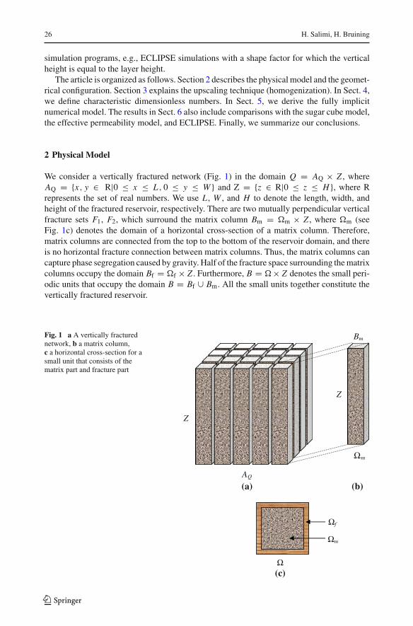
We consider a vertically fractured network (Fig. 1) in the domain Q = AQ × Z , whereAQ = {x, y ∈ R|0 ≤ x ≤ L , 0 ≤ y ≤ W } and Z = {z ∈ R|0 ≤ z ≤ H}, where Rrepresents the set of real numbers. We use L , W , and H to denote the length, width, andheight of the fractured reservoir, respectively. There are two mutually perpendicular verticalfracture sets F1, F2, which surround the matrix column Bm = m × Z , where m (seeFig. 1c) denotes the domain of a horizontal cross-section of a matrix column. Therefore,matrix columns are connected from the top to the bottom of the reservoir domain, and thereis no horizontal fracture connection between matrix columns. Thus, the matrix columns cancapture phase segregation caused by gravity. Half of the fracture space surrounding the matrixcolumns occupy the domain Bf = f × Z . Furthermore, B = × Z denotes the small peri-odic units that occupy the domain B = Bf ∪ Bm. All the small units together constitute thevertically fractured reservoir.
Fig. 1 a A vertically fracturednetwork, b a matrix column,c a horizontal cross-section for asmall unit that consists of thematrix part and fracture part
(a)
(c)
(b)AQ
Z
Bm
Ωm
Z
Ωf
Ω
Ωm
123

Upscaling in Vertically Fractured Oil Reservoirs 27
We simulate the injection of water into a vertically fractured oil reservoir. We apply conti-nuity of capillary pressure and continuity of fluid flow as boundary conditions on the verticalinterfaces between fracture and matrix columns. Flux continuity follows from fluid conserva-tion at the interface between fracture and matrix. There is capillary pressure continuity at theboundary of fractures and matrix columns unless one of the phases either in the matrix or infracture is immobile (Van Duijn et al. 1995). Indeed when one of the phases is immobile, thepressure of that phase depends on local conditions and cannot be determined globally. Hence,the capillary pressure, which is the difference between the phase pressure of the non-wettingphase and wetting phase, can be discontinuous. However, as residual saturations do not flow,this presents no difficulties for the modeling. Continuity of force, and hence continuity ofphase pressures, implies continuity of capillary pressure when both phases are mobile.
Moreover, we incorporate the gravity effect directly inside the matrix columns. As a result,there is a net flow within the matrix columns. The symmetry of the fracture pattern in thehorizontal plane is such that the fracture permeability can be considered isotropic. We onlyconsider a two-phase (oil and water) incompressible flow where water viscosity, μw, and oilviscosity, μo, are assumed to be constant. As the main purpose of this article is to illustrateonly the essential concepts, we assume that the fracture permeability is isotropic but thisassumption can be easily relaxed (see below).
2.1 Model Equations
We use the two-phase (α = o,w) extension of Darcy’s law for constant fluid densities:
u∗αf = −k∗
f krα,f
μαf∇ (Pαf + ραgz) := −λ∗
αf∇αf ,
uαm = −kmkrα,m
μαm∇αm := −λαm∇αm.
(1)
In these equations, the superscript (∗) denotes the intrinsic (local) fracture properties. Theintrinsic fracture permeability evaluated inside the fracture is denoted by k∗
f . We define theintrinsic fracture permeability k∗
f based on the fracture aperture. The matrix permeability isdenoted by km. Relative permeabilities are denoted by krw,ζ and kro,ζ , where ζ = f, m indi-cates the fracture or matrix systems. Here P is the pressure, ρ is the fluid density, g is thegravity acceleration factor, and z is the vertical upward direction. We define a phase mobilityλα = kkrα/μα as the ratio between the phase permeability and fluid viscosity. The phasepotential α is equal to the pressure plus the gravity term.
The mass conservation equation reads
∂
∂t
(ϕζ ραζ Sαζ
) + ∇ · (uαζ ραζ
) = 0, (2)
where ϕ is the porosity and Sα is the phase saturation. We obtain the governing equationsdescribing incompressible two-phase flow by combining Darcy’s Law (Eq. 1) and the massconversation (Eq. 2)
∂
∂t
(ϕ∗
f ραf Sαf) = ∇ · (
ραfλ∗αf∇αf
)in f , (3)
and
∂
∂t(ϕmραm Sαm) = ∇ · (ραmλαm∇αm) in m. (4)
123
28 H. Salimi, H. Bruining
We define a capillary pressure Pc = Po − Pw. At the interface between the fracture andmatrix systems, there is continuity of water and oil flow
(ραfλ
∗αf∇αf
) · n = (ραmλαm∇αm) · n on ∂m, (5)
where n denotes the outward unit normal vector to the surface (∂m) pointing from thematrix to the fracture. At the interface, there is also continuity of capillary pressure.
3 Upscaling Technique
We start with two-phase flow equations at the local scale to obtain the upscaled equations for avertically fractured reservoir at the global scale using homogenization theory. The upscalingtechnique (homogenization) consists of five major steps.
The first step in the homogenization is the subdivision of the horizontal coordinates of thevertically fractured reservoir into two scales (see Fig. 1): local (small units) scale of size (l)and the global scale of size (L) that is much larger than the local scale. This implies that acondition for the application of homogenization is that separation of scales is possible. Ourchoice for the small unit (SU) scale is a single matrix column of which vertical faces aresurrounded by fractures and its horizontal faces (e.g., top and bottom) are connected to thecap and base rock. We define L as the dimension of the grid block scale. Note that eachgrid block consists of a few hundred small units. We define a scaling ratio ε = l/L betweenthe local scale and the global scale. A very large difference between the size of the globalscale (grid block) and the local scale (SU) in addition to the low permeability of matrixcolumns, suggests that the oil flux from the matrix columns to fractures only leads to localscale variations of the fracture potential. As a consequence of the separation of scales, anyspace dependent quantity required to describe the physical process is a function of these twoscales. Therefore, we can split the gradient operator (∇) into a global scale (big) term, ∇b,and a local scale (small) term, ∇s, where ∇ = ∇b + ∇s. The matrix equation acts at thelocal scale. Thus, we do not apply the splitting procedure to the matrix domain. However,in a vertically fractured reservoir, there is no separation of scales in the vertical directionbecause the global scale is the same as the local scale. Therefore, we only apply the splittingprocedure to the x- and y-component of the fracture gradient operator. After applying thisstep to Eqs. 3–5, they read
∂∂t
(ϕ∗
f Sαf) = ∇b,xy · λ∗
αf
(∇b,xyαf + ∇s,xyαf)
+∇s,xy · λ∗αf
(∇b,xyαf + ∇s,xyαf)
+∇z · (λ∗
αf∇zαf)
in f , (6)∂∂t (ϕm Sαm) = ∇s,xy · (
λαm∇s,xyαm)
+∇z · (λαm∇zαm) in m, (7)(λ∗
αf
(∇b,xy + ∇s,xy,∇z)αf
) · n = (λαm
(∇s,xy,∇z)αm
) · n on ∂m. (8)
Equations 3–5 have ρα as a common factor; therefore, it can be dropped in Eqs. 6–8.The second step in the homogenization technique is writing the equations at the local scale
in a dimensionless form using characteristic reference quantities. In our model, we use l andL as the characteristic lengths for the differentiation. This results in ∇D = ∇b + ε−1∇s. Thereference potential, R, is the potential difference between the injection and production well(�). tR = L2μ/(k�) acts as the reference time for both the fracture and matrix systems.
123
Upscaling in Vertically Fractured Oil Reservoirs 29
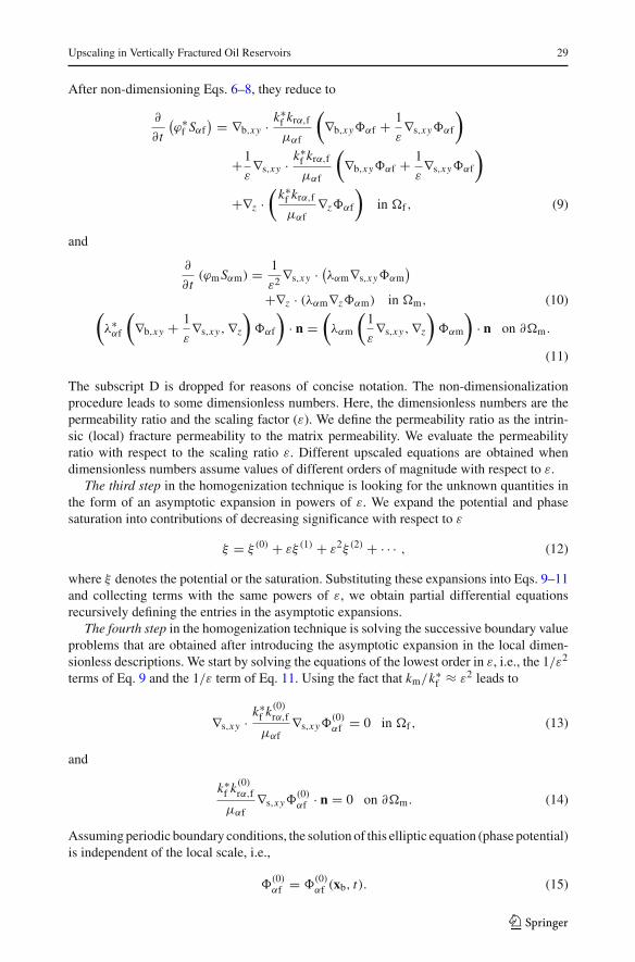
After non-dimensioning Eqs. 6–8, they reduce to
∂
∂t
(ϕ∗
f Sαf) = ∇b,xy · k∗
f krα,f
μαf
(∇b,xyαf + 1
ε∇s,xyαf
)
+1
ε∇s,xy · k∗
f krα,f
μαf
(∇b,xyαf + 1
ε∇s,xyαf
)
+∇z ·(
k∗f krα,f
μαf∇zαf
)in f , (9)
and
∂
∂t(ϕm Sαm) = 1
ε2 ∇s,xy · (λαm∇s,xyαm
)
+∇z · (λαm∇zαm) in m, (10)(
λ∗αf
(∇b,xy + 1
ε∇s,xy,∇z
)αf
)· n =
(λαm
(1
ε∇s,xy,∇z
)αm
)· n on ∂m.
(11)
The subscript D is dropped for reasons of concise notation. The non-dimensionalizationprocedure leads to some dimensionless numbers. Here, the dimensionless numbers are thepermeability ratio and the scaling factor (ε). We define the permeability ratio as the intrin-sic (local) fracture permeability to the matrix permeability. We evaluate the permeabilityratio with respect to the scaling ratio ε. Different upscaled equations are obtained whendimensionless numbers assume values of different orders of magnitude with respect to ε.
The third step in the homogenization technique is looking for the unknown quantities inthe form of an asymptotic expansion in powers of ε. We expand the potential and phasesaturation into contributions of decreasing significance with respect to ε
ξ = ξ (0) + εξ (1) + ε2ξ (2) + · · · , (12)
where ξ denotes the potential or the saturation. Substituting these expansions into Eqs. 9–11and collecting terms with the same powers of ε, we obtain partial differential equationsrecursively defining the entries in the asymptotic expansions.
The fourth step in the homogenization technique is solving the successive boundary valueproblems that are obtained after introducing the asymptotic expansion in the local dimen-sionless descriptions. We start by solving the equations of the lowest order in ε, i.e., the 1/ε2
terms of Eq. 9 and the 1/ε term of Eq. 11. Using the fact that km/k∗f ≈ ε2 leads to
∇s,xy · k∗f k(0)
rα,f
μαf∇s,xy
(0)αf = 0 in f , (13)
and
k∗f k(0)
rα,f
μαf∇s,xy
(0)αf · n = 0 on ∂m. (14)
Assuming periodic boundary conditions, the solution of this elliptic equation (phase potential)is independent of the local scale, i.e.,
(0)αf =
(0)αf (xb, t). (15)
123
30 H. Salimi, H. Bruining
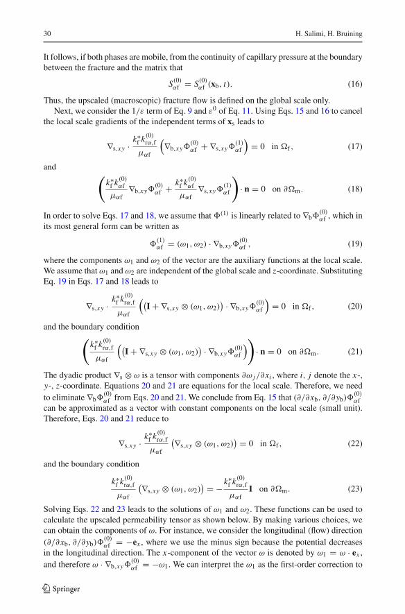
It follows, if both phases are mobile, from the continuity of capillary pressure at the boundarybetween the fracture and the matrix that
S(0)αf = S(0)
αf (xb, t). (16)
Thus, the upscaled (macroscopic) fracture flow is defined on the global scale only.Next, we consider the 1/ε term of Eq. 9 and ε0 of Eq. 11. Using Eqs. 15 and 16 to cancel
the local scale gradients of the independent terms of xs leads to
∇s,xy · k∗f k(0)
rα,f
μαf
(∇b,xy
(0)αf + ∇s,xy
(1)αf
)= 0 in f , (17)
and(
k∗f k(0)
αf
μαf∇b,xy
(0)αf + k∗
f k(0)αf
μαf∇s,xy
(1)αf
)
· n = 0 on ∂m. (18)
In order to solve Eqs. 17 and 18, we assume that (1) is linearly related to ∇b(0)αf , which in
its most general form can be written as
(1)αf = (ω1, ω2) · ∇b,xy
(0)αf , (19)
where the components ω1 and ω2 of the vector are the auxiliary functions at the local scale.We assume that ω1 and ω2 are independent of the global scale and z-coordinate. SubstitutingEq. 19 in Eqs. 17 and 18 leads to
∇s,xy · k∗f k(0)
rα,f
μαf
((I + ∇s,xy ⊗ (ω1, ω2)
) · ∇b,xy(0)αf
)= 0 in f , (20)
and the boundary condition(
k∗f k(0)
rα,f
μαf
((I + ∇s,xy ⊗ (ω1, ω2)
) · ∇b,xy(0)αf
))
· n = 0 on ∂m. (21)
The dyadic product ∇s ⊗ ω is a tensor with components ∂ω j/∂xi , where i, j denote the x-,y-, z-coordinate. Equations 20 and 21 are equations for the local scale. Therefore, we needto eliminate ∇b
(0)αf from Eqs. 20 and 21. We conclude from Eq. 15 that (∂/∂xb, ∂/∂yb)
(0)αf
can be approximated as a vector with constant components on the local scale (small unit).Therefore, Eqs. 20 and 21 reduce to
∇s,xy · k∗f k(0)
rα,f
μαf
(∇s,xy ⊗ (ω1, ω2)) = 0 in f , (22)
and the boundary condition
k∗f k(0)
rα,f
μαf
(∇s,xy ⊗ (ω1, ω2)) = −k∗
f k(0)rα,f
μαfI on ∂m. (23)
Solving Eqs. 22 and 23 leads to the solutions of ω1 and ω2. These functions can be used tocalculate the upscaled permeability tensor as shown below. By making various choices, wecan obtain the components of ω. For instance, we consider the longitudinal (flow) direction(∂/∂xb, ∂/∂yb)
(0)αf = −ex , where we use the minus sign because the potential decreases
in the longitudinal direction. The x-component of the vector ω is denoted by ω1 = ω · ex ,and therefore ω · ∇b,xy
(0)αf = −ω1. We can interpret the ω1 as the first-order correction to
123
Upscaling in Vertically Fractured Oil Reservoirs 31
the potential (0) when the system is subjected to a unit global gradient in the x-direction.The behavior of ω1 is therefore a measure of the potential fluctuation caused by the non-homogeneous nature of a porous medium.
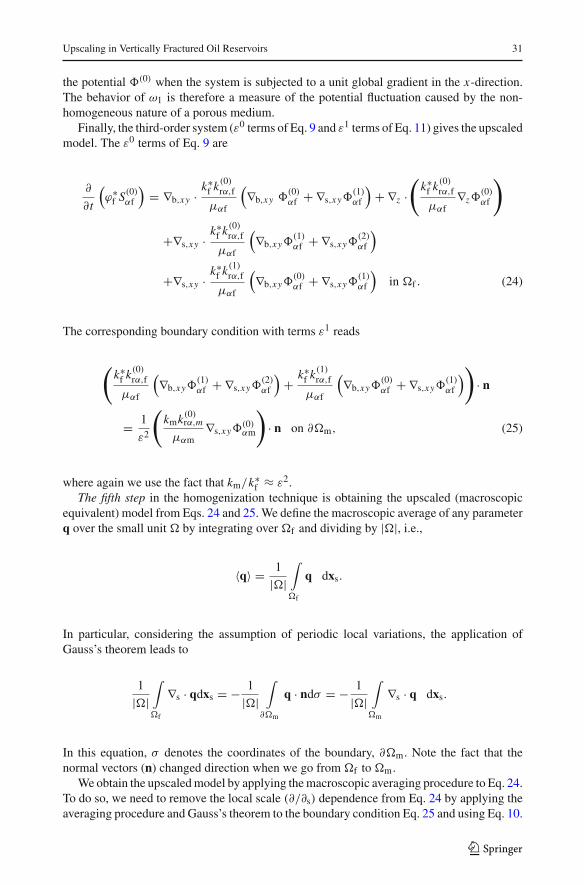
Finally, the third-order system (ε0 terms of Eq. 9 and ε1 terms of Eq. 11) gives the upscaledmodel. The ε0 terms of Eq. 9 are
∂
∂t
(ϕ∗
f S(0)αf
)= ∇b,xy · k∗
f k(0)rα,f
μαf
(∇b,xy
(0)αf + ∇s,xy
(1)αf
)+ ∇z ·
(k∗
f k(0)rα,f
μαf∇z
(0)αf
)
+∇s,xy · k∗f k(0)
rα,f
μαf
(∇b,xy
(1)αf + ∇s,xy
(2)αf
)
+∇s,xy · k∗f k(1)
rα,f
μαf
(∇b,xy
(0)αf + ∇s,xy
(1)αf
)in f . (24)
The corresponding boundary condition with terms ε1 reads
(k∗
f k(0)rα,f
μαf
(∇b,xy
(1)αf + ∇s,xy
(2)αf
)+ k∗
f k(1)rα,f
μαf
(∇b,xy
(0)αf + ∇s,xy
(1)αf
))
· n
= 1
ε2
(kmk(0)
rα,m
μαm∇s,xy
(0)αm
)
· n on ∂m, (25)
where again we use the fact that km/k∗f ≈ ε2.
The fifth step in the homogenization technique is obtaining the upscaled (macroscopicequivalent) model from Eqs. 24 and 25. We define the macroscopic average of any parameterq over the small unit by integrating over f and dividing by ||, i.e.,
〈q〉 = 1
||∫
f
q dxs.
In particular, considering the assumption of periodic local variations, the application ofGauss’s theorem leads to
1
||∫
f
∇s · qdxs = − 1
||∫
∂m
q · ndσ = − 1
||∫
m
∇s · q dxs.
In this equation, σ denotes the coordinates of the boundary, ∂m. Note the fact that thenormal vectors (n) changed direction when we go from f to m.
We obtain the upscaled model by applying the macroscopic averaging procedure to Eq. 24.To do so, we need to remove the local scale (∂/∂s) dependence from Eq. 24 by applying theaveraging procedure and Gauss’s theorem to the boundary condition Eq. 25 and using Eq. 10.
123

32 H. Salimi, H. Bruining
The third and fourth terms after the equal sign of Eq. 24 become
1
||∫
f
{
∇s,xy · k∗f k(0)
rα,f
μαf
(∇b,xy
(1)αf + ∇s,xy
(2)αf
)
+ ∇s,xy · k∗f k(1)
rα,f
μαf
(∇b,xy
(0)αf + ∇s,xy
(1)αf
)}
dxs
= − 1
||∫
∂m
{
∇s,xy · k∗f k(0)
rα,f
μαf
(∇b,xy
(1)αf + ∇s,xy
(2)αf
)
+ ∇s,xy · k∗f k(1)
rα,f
μαf
(∇b,xy
(0)αf + ∇s,xy
(1)αf
)}
.ndσ
= − 1
||∫
∂m
1
ε2
(kmk(0)
rα,m
μαm∇s,xy
(0)αm
)
.ndσ
= − 1
||∫
m
1
ε2
{
∇s,xy .
(kmk(0)
rα,m
μαm∇s,xy
(0)αm
)}
dxs
= − 1
||∫
m
{∂
∂t
(ϕm S(0)
αm
)− ∇z ·
(λ(0)
αm∇z(0)αm
)}dxs. (26)
This term is the exchange term of fluid flow at the interface between the fracture and matrix.In other words, it acts as an internal matrix source term in the upscaled fracture model, whichmeans it shows how much water imbibes to the matrix and how much oil is fed to the fractureby the matrix columns.
The first and second terms after the equal sign of Eq. 24 can be written with Eq. 19 as
1
||∫
f
{
∇b,xy · k∗f k(0)
rα,f
μαf
(∇b,xy
(0)αf + ∇s,xy
(1)αf
)+ ∇z ·
(k∗
f k(0)rα,f
μαf∇z
(0)αf
)}
dxs
= 1
||∫
f
{
∇b,xy ·(
k∗f k(0)
rα,f
μαf
(I + ∇s,xy ⊗ (ω1, ω2)
) · ∇b,xy(0)αf
)
+∇z ·(
k∗f k(0)
rα,f
μαf∇z
(0)αf
)}
dxs
= 1
||∫
f
{
∇b ·(
k∗f k(0)
rα,f
μαf(I + ∇s ⊗ (ω1, ω2, 0)) · ∇b
(0)αf
)}
dxs
= ∇b ·(
kf k(0)rα,f
μαf∇b
(0)αf
)
, (27)
where we define the effective fracture permeability tensor as follows:
kf = 1
||∫
f
k∗f (I + ∇s ⊗ (ω1, ω2, 0)) dxs. (28)
123
Upscaling in Vertically Fractured Oil Reservoirs 33
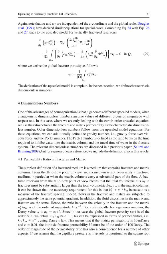
Again, note that ω1 and ω2 are independent of the z-coordinate and the global scale. Douglaset al. (1993) have derived similar equations for special cases. Combining Eq. 24 with Eqs. 26and 27 leads to the upscaled model for vertically fractured reservoirs
∂
∂t
(ϕf S(0)
αf
)− ∇b ·
(kf k(0)
rα,f
μαf∇b
(0)αf
)
+ 1
||∫
m
{∂
∂t
(ϕm S(0)
αm
)− ∂
∂z
(λ(0)
αm∂
∂z(0)
αm
)}dxs = 0 in Q, (29)
where we derive the global fracture porosity as follows:
ϕf = 1
||∫
f
ϕ∗f dxs.
The derivation of the upscaled model is complete. In the next section, we define characteristicdimensionless numbers.
4 Dimensionless Numbers
One of the advantages of homogenization is that it generates different upscaled models, whencharacteristic dimensionless numbers assume values of different orders of magnitude withrespect to ε. In this case, where we are only dealing with the zeroth-order upscaled equation,we use the ratio between the fracture and matrix permeability as the characteristic dimension-less number. Other dimensionless numbers follow from the upscaled model equations. Forthese equations, we can additionally define the gravity number, i.e., gravity force over vis-cous force and the Peclet number. The Peclet number is defined as the ratio between the timerequired to imbibe water into the matrix column and the travel time of water in the fracturesystem. The relevant dimensionless numbers are discussed in a previous paper (Salimi andBruining 2009), but for reasons of easy reference, we include the definition also in this article.
4.1 Permeability Ratio in Fractures and Matrix
The simplest definition of a fractured medium is a medium that contains fractures and matrixcolumns. From the fluid-flow point of view, such a medium is not necessarily a fracturedmedium, in particular when the matrix columns carry a substantial part of the flow. A frac-tured reservoir from the fluid-flow point of view means that the total volumetric flux uf infractures must be substantially larger than the total volumetric flux um in the matrix columns.It can be shown that the necessary requirement for this is that k∗
f ≈ ε−2 km because ε is ameasure of the fracture spacing. Indeed, flows in the fracture and matrix are subjected toapproximately the same potential gradient. In addition, the fluid viscosities in the matrix andfracture are the same. Hence, the ratio between the velocity in the fracture and the matrixu∗
f /um is of the order of magnitude ≈ ε−2. For a statistically homogeneous medium, theDarcy velocity is uf ≈ ϕf u∗
f . Since in our case the global fracture porosity (ϕf ) is of theorder ≈ ε, we obtain uf/um ≈ ε−1. This can be expressed in terms of permeabilities, i.e.,kf/km ≈ ε−1, using Darcy’s law. This means that if the matrix permeability is 10 mDarcyand ε ≈ 0.01, the intrinsic fracture permeability k∗
f must be of the order of 100 Darcy. Theorder of magnitude of the permeability ratio has also a consequence for a number of otheraspects. If we assume that the capillary pressure is inversely proportional to the square root
123
34 H. Salimi, H. Bruining
of the permeability√
k, it means that for the same saturation values, the capillary pressurein the matrix columns is 100 times as large as in the fracture.
4.2 Peclet Number
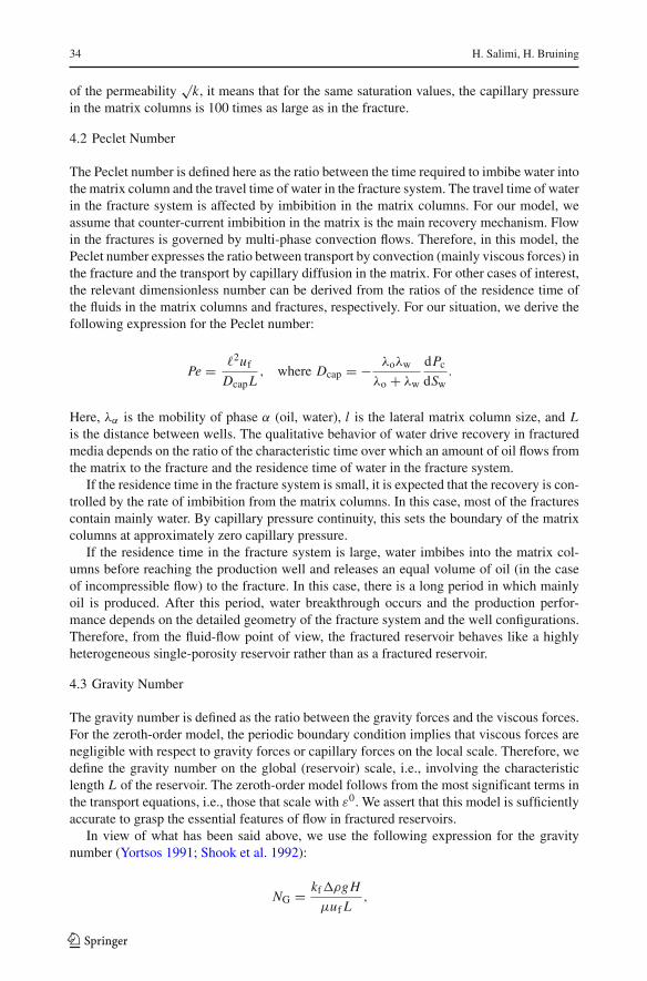
The Peclet number is defined here as the ratio between the time required to imbibe water intothe matrix column and the travel time of water in the fracture system. The travel time of waterin the fracture system is affected by imbibition in the matrix columns. For our model, weassume that counter-current imbibition in the matrix is the main recovery mechanism. Flowin the fractures is governed by multi-phase convection flows. Therefore, in this model, thePeclet number expresses the ratio between transport by convection (mainly viscous forces) inthe fracture and the transport by capillary diffusion in the matrix. For other cases of interest,the relevant dimensionless number can be derived from the ratios of the residence time ofthe fluids in the matrix columns and fractures, respectively. For our situation, we derive thefollowing expression for the Peclet number:
Pe = �2uf
DcapL, where Dcap = − λoλw
λo + λw
dPc
dSw.
Here, λα is the mobility of phase α (oil, water), l is the lateral matrix column size, and Lis the distance between wells. The qualitative behavior of water drive recovery in fracturedmedia depends on the ratio of the characteristic time over which an amount of oil flows fromthe matrix to the fracture and the residence time of water in the fracture system.
If the residence time in the fracture system is small, it is expected that the recovery is con-trolled by the rate of imbibition from the matrix columns. In this case, most of the fracturescontain mainly water. By capillary pressure continuity, this sets the boundary of the matrixcolumns at approximately zero capillary pressure.
If the residence time in the fracture system is large, water imbibes into the matrix col-umns before reaching the production well and releases an equal volume of oil (in the caseof incompressible flow) to the fracture. In this case, there is a long period in which mainlyoil is produced. After this period, water breakthrough occurs and the production perfor-mance depends on the detailed geometry of the fracture system and the well configurations.Therefore, from the fluid-flow point of view, the fractured reservoir behaves like a highlyheterogeneous single-porosity reservoir rather than as a fractured reservoir.
4.3 Gravity Number
The gravity number is defined as the ratio between the gravity forces and the viscous forces.For the zeroth-order model, the periodic boundary condition implies that viscous forces arenegligible with respect to gravity forces or capillary forces on the local scale. Therefore, wedefine the gravity number on the global (reservoir) scale, i.e., involving the characteristiclength L of the reservoir. The zeroth-order model follows from the most significant terms inthe transport equations, i.e., those that scale with ε0. We assert that this model is sufficientlyaccurate to grasp the essential features of flow in fractured reservoirs.
In view of what has been said above, we use the following expression for the gravitynumber (Yortsos 1991; Shook et al. 1992):
NG = kf�ρgH
μuf L,
123

Upscaling in Vertically Fractured Oil Reservoirs 35
where H is the height of the reservoir. As the Darcy velocity uf is increasing, the viscousforces of the fracture system start to dominate gravity forces in the fracture system. Onthe other hand, when the injection velocity is small, gravity forces become dominant in thefracture system. This means that for this case, water tends to under-ride especially for highmobility ratios and gravity segregation happens.
5 Numerical Solution
The numerical procedure described below is an extension of the method used by Arbogast(1997) and Salimi and Bruining (2009) for the sugar cube model. The difficulty arises dueto a coupling of flow in the vertical direction, which is important in the aggregated columnmodel. From the computational point of view, we consider a matrix column associated witheach point in the base plane of the reservoir. The horizontal cross-sectional position of anypoint rb = (xb, yb, zb) ∈ Q, is denoted by r′
b = (xb, yb) ∈ AQ. The matrix column atr′
b = (xb, yb) ∈ AQ is denoted by Bm(r′b) = m
(r′
b
) × H , where this matrix column isrepresentative of matrix columns in the vicinity of r′. We formulate our numerical methodin terms of the water potential, the capillary pressure, and the water saturation. Here, wealso define the capillary potential c = Pc + (ρo − ρw) gz. We assume that all externalsources, i.e., the production and injection wells, influence only the fractures. Equations 30and 32 below are called the saturation equations, and the sums over the phases of each of thetwo-phase equations are 31 and 33, the pressure equations. Then, the upscaled equations inthe fractured reservoir are
∂
∂t(ϕf Swf ) − ∇b · (λwf∇bwf )
+ 1
||∫
m
{∂
∂t(ϕm Swm) − ∂
∂z
(λwm
∂
∂zwm
)}dxs = qext,w in Q, (30)
−∇b · ((λwf + λof ) ∇bwf + λof∇bcf )
+ 1
||∫
m
{− ∂
∂z
((λwm + λom)
∂
∂zwm + λom
∂
∂zcm
)}dxs = qext,w + qext,o in Q,
(31)
where qext,w and qext,o are the external flow rates that come from the production and injectionwells. The superscript (0) is dropped for reasons of concise notation. The equations on thematrix columns at r′
b are
∂
∂t(ϕm Swm) − ∇s · (λwm∇swm) = 0 in Bm(r ′
b), (32)
−∇s · ((λwm + λom) ∇s wm + λom∇scm) = 0 in Bm(r ′b), (33)
The boundary conditions on the vertical faces of the matrix columns read
wm (t, xb, xs) = wf (t, xb) , and cm (t, xb, xs) = cf (t, xb) . (34)
There are no-flow boundary conditions on the top and bottom of the entire fracturedreservoir, i.e.,
−λαζ ∇αζ · n = 0, α = w, o, and ζ = f, m. (35)
123

36 H. Salimi, H. Bruining
Initially, there is capillary–gravity equilibrium both in the fracture system and in the matrixcolumn. This means that the fluid exchange term between fracture and matrix is zero initially.Since initial oil in place is known, we determine the initial fracture water potential by solvingthe fracture pressure equation (Eq. 31). Due to equilibrium, we can solve the matrix pressureequation (Eq. 33) to obtain the initial matrix water potential.
Equations 30–35 cannot be solved sequentially or explicitly, because a small change inthe boundary values on each matrix column can cause flow of a volume of fluid that is largein comparison to the volume of the fractures (Douglas et al. 1991). In other words, the matrixabsorbs more fluid from the surrounding fractures in one-step than can be resident there.Part of the excess volume in the matrix is returned to the fractures in the next step, how-ever, violating mass conservation. Therefore, the fracture–matrix interaction must be handledimplicitly.
We use a backward Euler, time approximation for the complete system of Eqs. 30–35. Wefurther use a fully implicit finite volume approach and first-order upwind scheme for spatialdiscretization. To facilitate the implementation of the no-flow boundary conditions and thecontinuity conditions of the potentials along the fracture–matrix interfaces, we discretize thespace variables in a cell-centered manner in the fractures and also cell-centered with respectto z in the matrix columns. However, the discretization in the xs and ys are vertex-centered.In this work, we use uniform grid cells in the fractures and in each matrix column. Fromthe computational perspective, we consider a case in which the vertical discretization in thematrix columns coincides with that in the fractures.
We discretize Q into Nxf × Nyf × Nzf grid cells, each grid cell of size dxf × dyf × dzf .The center of the fracture cell p = (px , py, pz) is then
xbp = ((px − 1/2)dxf , (py − 1/2)dyf , (pz − 1/2)dzf
),
and the set of all fracture grid cell centers is
Nf = {xbpi
: pi = 1, 2, 3, . . . , Nif , i = x, y, z}.
This reduces the system of the equations to a fully discrete, three-dimensional problem. Wedenote the vectors of unknowns in the fracture by
�nwf = {
nwf,i , i = 1, 2, 3, . . . , Nxf × Nyf × Nzf
},
�Snwf = {
Snwf,i , i = 1, 2, 3, . . . , Nxf × Nyf × Nzf
},
where superscript n denotes the time level n. In the vector, the potentials and saturations arestacked behind each other.
At each xbp ∈ Nf , there is a representative matrix column Bm(xbp′) = (0, dxm Nxm) ×(0, dym Nym) × (0, dzf Nzf ), where p′ = (px , py) is the projection of p on the x–y plane.Then, the center point of each matrix cell c = (cx , cy, cz) is
xsp′ = (cx dxm,p′ , cydym,p′ , (cz − 1/2)dxf )
and the set of all matrix cell center points at fracture point p is given by
Nm,p′ = {xsp′,ci : ci = 0, 1, . . . , Nim,p′ , i = x, y;cz = 1, 2, . . . , Nzf
}.
Then, associated with each grid point i = 1, 2, . . ., Nxf × Nyf × Nzf , we have two series ofmatrix unknowns
�nwm,i ′ =
{n
wm,i ′ j , i ′ = 1, 2, . . . , Nxf × Nyf , j = 1, 2, 3, . . . , Nxm × Nym × Nzf
},
�Snwm,i ′ =
{Sn
wm,i ′ j , i ′ = 1, 2, . . . , Nxf × Nyf , j = 1, 2, 3, . . . , Nxm × Nym × Nzf
},
123
Upscaling in Vertically Fractured Oil Reservoirs 37
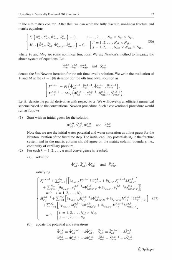
in the mth matrix column. After that, we can write the fully discrete, nonlinear fracture andmatrix equations
⎧⎪⎨
⎪⎩
Fi
( �nwf ,
�Snwf ,
�nwm, �Sn
wm
)= 0, i = 1, 2, . . . , Nxf × Nyf × Nzf ,
Mi ′ j
( �nwf ,
�Snwf ,
�nwm,i ′ ,
�Snwm,i ′
)= 0,
{i ′ = 1, 2, . . . , Nxf × Nyf ,
j = 1, 2, . . . , Nxm × Nym × Nzf ,
(36)
where Fi and Mi ′ j are some nonlinear functions. We use Newton’s method to linearize theabove system of equations. Let
�n,kwf , �Sn,k
wf , �n,kwm, and �Sn,k
wm,
denote the kth Newton iteration for the nth time level’s solution. We write the evaluation ofF and M at the (k − 1)th iteration for the nth time level solution as
⎧⎨
⎩
Fn,k−1i = Fi
( �n,k−1wf , �Sn,k−1
wf , �n,k−1wm , �Sn,k−1
wm
),
Mn,k−1i ′ j = Mi ′ j
( �n,k−1wf , �Sn,k−1
wf , �n,k−1wm,i ′ ,
�Sn,k−1wm,i ′
).
Let ∂π denote the partial derivative with respect to π . We will develop an efficient numericalscheme based on the conventional Newton procedure. Such a conventional procedure wouldrun as follows:
(1) Start with an initial guess for the solution
�n,0wf , �Sn,0
wf , �n,0wm, and �Sn,0
wm.
Note that we use the initial water potential and water saturation as a first guess for theNewton iteration of the first time step. The initial capillary potentials c in the fracturesystem and in the matrix column should agree on the matrix column boundary, i.e.,continuity of capillary pressure.
(2) For each k = 1, 2, . . . , n until convergence is reached:
(a) solve for
�n,kwf , �Sn,k
wf , �n,kwm, and �Sn,k
wm,
satisfying⎧⎪⎪⎪⎪⎪⎪⎪⎪⎪⎪⎪⎪⎪⎨
⎪⎪⎪⎪⎪⎪⎪⎪⎪⎪⎪⎪⎪⎩
Fn,k−1i + ∑Nf
i ′′=1
{[∂wf,i ′′ Fn,k−1
i δn,kwf,i ′′ + ∂Swf,i ′′ Fn,k−1
i δSn,kwf,i ′′
]
+ ∑Nmj ′=1
[∂wm,i ′′ j ′ Fn,k−1
i δn,kwm,i ′′ j ′ + ∂Swm,i ′′ j ′ Fn,k−1
i δSn,kwm,i ′′ j ′
]}
= 0, i = 1, 2, . . . , Nf ,
Mn,k−1i ′ j + ∑Nzf
l=1
[∂wf,(i ′,l) Mn,k−1
i ′ j δn,kwf,(i ′,l) + ∂Swf,(i ′,l) Mn,k−1
i ′ j δSn,kwf,(i ′,l)
]
+∑Nmj ′=1
[∂wm,i ′ j ′ Mn,k−1
i ′ j δn,kwm,i ′ j ′ + ∂Swm,i ′ j ′ Mn,k−1
i ′ j δSn,kwm,i ′ j ′
]
= 0,
{i ′ = 1, 2, . . . , Nxf × Nyf ,
j = 1, 2, . . . , Nm,
(37)
(b) update the potential and saturations
�n,kwf = �n,k−1
wf + δ �n,kwf , �Sn,k
wf = �Sn,k−1wf + δ �Sn,k
wf ,
�n,kwm = �n,k−1
wm + δ �n,kwm, �Sn,k
wm = �Sn,k−1wm + δ �Sn,k
wm.
123

38 H. Salimi, H. Bruining
This would complete the algorithm for a time step. The above linear system (Eq. 37) involvesthe solution of a (2×(Nf + Nxf × Nyf × Nm))×(2×(Nf + Nxf × Nyf × Nm)) matrix for eachNewton iteration at a time step, which is computationally expensive. Within the linearizedNewton problem (Eq. 37), the matrix solutions in the i th column depend on
n,kwf,(i ′,l) and
Sn,kwf,(i ′,l), where l = 1, 2, . . ., Nzf . In other words, the matrix solution in the i th column only
depends on all the fracture cells surrounding the matrix column of interest. It is thereforepossible to develop an efficient numerical scheme by decoupling the matrix and fractureproblems without affecting the implicit nature of the scheme. We replace the matrix problemin Eq. 37 by the following three types of problems for
(δ �n,m
wm,(i ′,l), δ�Sn,m
wm,(i ′,l)
),
(δ �n,m
wm,(i ′,l), δ�Sn,m
wm,(i ′,l)
), and
(δ �n,m
wm,i ′ , δ�Sn,m
wm,i ′)
,
where δ’s, δ’s, and δ’s satisfy three types of problems as follows:First, for each i ′ = 1, 2, . . . , Nxf × Nyf and j = 1, 2, 3, . . . , Nm,
Mn,k−1i ′ j +
Nm∑
j ′=1
[∂wm,i ′ j ′ Mn,k−1
i ′ j δn,kwm,i ′ j ′ + ∂Swm,i ′ j ′ Mn,k−1
i ′ j δSn,kwm,i ′ j ′
]= 0. (38)
Second, for l = 1, . . ., Nzf ,
∂wf,(i ′,l) Mn,k−1i ′ j +
Nm∑
j ′=1
[∂wm,i ′ j ′ Mn,k−1
i ′ j δn,kwm,(i ′,l), j ′ + ∂Swm,i ′ j ′ Mn,k−1
i ′ j δSn,kwm,(i ′,l), j ′
]= 0.
(39)
Third, for l = 1, . . . , Nzf ,
∂Swf,(i ′,l) Mn,k−1i ′ j +
Nm∑
j ′=1
[∂wm,i ′ j ′ Mn,k−1
i ′ j δn,kwm,(i ′,l), j ′ + ∂Swm,i ′ j ′ Mn,k−1
i ′ j δSn,kwm,(i ′,l), j ′
]= 0.
(40)
If we multiply Eq. 39 by δn,kwf,(i ′,l) and Eq. 40 by δSn,k
wf,(i ′,l) and then add these equationsto Eq. 38, the result is identical to the matrix problem in Eq. 37. As a result, the matrixunknowns can be calculated by
δn,kwm,i ′ j = δ
n,kwm,i ′ j +
Nzf∑
l=1
(δ
n,kwm,(i ′,l), jδ
n,kwf,(i ′,l) + δ
n,kwm,(i ′,l), jδSn,k
wf,(i ′,l)
), (41)
and
δSn,kwm,i ′ j = δSn,k
wm,i ′ j +Nzf∑
l=1
(δSn,k
wm,(i ′,l), jδn,kwf,(i ′,l) + δSn,k
wm,(i ′,l), jδSn,kwf,(i ′,l)
). (42)
Equations 38–40 can be solved independently of the fracture system. Thus, we modify step2(a) of the Newton Algorithm by first solving Eqs. 38–40. The changes in the fractureunknowns are then given by solving the fracture equations of 37, using implicitly definitionof Eqs. 41 and 42. Subsequently, we explicitly use the changes in the fracture unknowns andEqs. 41 and 42 to update the matrix δ-potential and matrix δ-saturation. Finally, the Newtoniteration can be continued. This efficient numerical method is inexpensive as it only involvesthe solution of many (2× Nm)× (2× Nm) matrices and the solution of a (2× Nf )× (2× Nf )
matrix as opposed to a single big matrix.
123
Upscaling in Vertically Fractured Oil Reservoirs 39
6 Results and Discussion
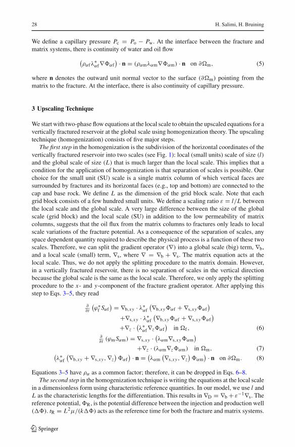
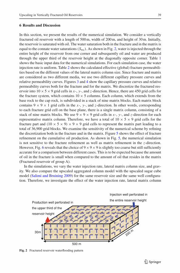
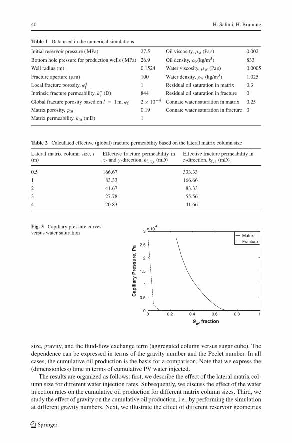
In this section, we present the results of the numerical simulation. We consider a verticallyfractured oil reservoir with a length of 500 m, width of 200 m, and height of 30 m. Initially,the reservoir is saturated with oil. The water saturation both in the fracture and in the matrix isequal to the connate water saturations (Swc). As shown in Fig. 2, water is injected through theentire height of the reservoir from one corner and subsequently oil and water are producedthrough the upper third of the reservoir height at the diagonally opposite corner. Table 1shows the basic input data for the numerical simulations. For each simulation case, the waterinjection rate is uniform. Table 2 shows the calculated effective (global) fracture permeabili-ties based on the different values of the lateral matrix column size. Since fracture and matrixare considered as two different media, we use two different capillary pressure curves andrelative permeability curves. Figures 3 and 4 show the capillary pressure curves and relativepermeability curves both for the fracture and for the matrix. We discretize the fractured res-ervoir into 10 × 5 × 9 grid cells in x-, y-, and z-direction. Hence, there are 450 grid cells forthe fracture system, which contains 10 × 5 columns. Each column, which extends from thebase rock to the cap rock, is subdivided in a stack of nine matrix blocks. Each matrix blockcontains 9 × 9 × 1 grid cells in the x-, y-, and z-direction. In other words, correspondingto each fracture grid cell on the base plane, there is a single matrix column, consisting of astack of nine matrix blocks. We use 9 × 9 × 9 grid cells in x-, y-, and z-direction for eachrepresentative matrix column. Therefore, we have a total of 10 × 5 × 9 grid cells for thefracture part and (10 × 5 × 9) × 9 × 9 grid cells to represent the matrix part leading to atotal of 36,900 grid blocks. We examine the sensitivity of the numerical scheme by refiningthe discretization both in the fracture and in the matrix. Figure 5 shows the effect of fracturerefinement on the cumulative oil production. As shown in Fig. 5, the numerical simulationis not sensitive to the fracture refinement as well as matrix refinement in the z-direction.However, Fig. 6 reveals that the choice of 9 × 9 × 9 is slightly too coarse but still sufficientlyaccurate for a comparison between different cases. This is to be expected because the amountof oil in the fracture is small when compared to the amount of oil that resides in the matrix(Fractured reservoir of group A).
In the simulations, we vary the water injection rate, lateral matrix column size, and grav-ity. We also compare the upscaled aggregated column model with the upscaled sugar cubemodel (Salimi and Bruining 2009) for the same reservoir size and the same well configura-tion. Therefore, we investigate the effect of the water injection rate, lateral matrix column
30m
500 m
Injection well perforated in
the entire reservoir height Production well perforated in
the upper third of the
reservoir height
200 m
Fig. 2 Fractured reservoir waterflooding pattern
123
40 H. Salimi, H. Bruining
Table 1 Data used in the numerical simulations
Initial reservoir pressure ( MPa) 27.5 Oil viscosity, μo (Pa s) 0.002
Bottom hole pressure for production wells ( MPa) 26.9 Oil density, ρo(kg/m3) 833
Well radius (m) 0.1524 Water viscosity, μw (Pa s) 0.0005
Fracture aperture (µm) 100 Water density, ρw (kg/m3) 1,025
Local fracture porosity, ϕ∗f 1 Residual oil saturation in matrix 0.3
Intrinsic fracture permeability, k∗f (D) 844 Residual oil saturation in fracture 0
Global fracture porosity based on l = 1 m, ϕf 2 × 10⁻⁴ Connate water saturation in matrix 0.25
Matrix porosity, ϕm 0.19 Connate water saturation in fracture 0
Matrix permeability, km (mD) 1
Table 2 Calculated effective (global) fracture permeability based on the lateral matrix column size
Lateral matrix column size, l(m)
Effective fracture permeability inx- and y-direction, kf,xy (mD)
Effective fracture permeability inz-direction, kf,z (mD)
0.5 166.67 333.33
1 83.33 166.66
2 41.67 83.33
3 27.78 55.56
4 20.83 41.66
Fig. 3 Capillary pressure curvesversus water saturation
0 0.2 0.4 0.6 0.8 10
0.5
1
1.5
2
2.5
3 x 10 4
S w , fraction
a P
, e r
u
s s e r P
y r a l l i
p
a C
Matrix Fracture
size, gravity, and the fluid-flow exchange term (aggregated column versus sugar cube). Thedependence can be expressed in terms of the gravity number and the Peclet number. In allcases, the cumulative oil production is the basis for a comparison. Note that we express the(dimensionless) time in terms of cumulative PV water injected.
The results are organized as follows: first, we describe the effect of the lateral matrix col-umn size for different water injection rates. Subsequently, we discuss the effect of the waterinjection rates on the cumulative oil production for different matrix column sizes. Third, westudy the effect of gravity on the cumulative oil production, i.e., by performing the simulationat different gravity numbers. Next, we illustrate the effect of different reservoir geometries
123

Upscaling in Vertically Fractured Oil Reservoirs 41
Fig. 4 Relative permeabilitycurves versus water saturation
0 0.2 0.4 0.6 0.8 10
0.2
0.4
0.6
0.8
1
Sw, fraction
Rel
ativ
e P
erm
eab
ility
, fra
ctio
n
Oil in MatrixWater in MatrixOil in FractureWater in Fracture
Fig. 5 Effect of fracturediscretization on the cumulativeoil production
0 0.5 1 1.5 20
0.05
0.1
0.15
0.2
0.25
0.3
0.35
0.4
Time, PV
V
P
, n
o
i t c
u
d
o
r P
l i
O
e v i t a l u
m
u
C
10 × 5 × 9
10 × 5 × 12
10 × 5 × 15
Fig. 6 Effect of matrixdiscretization on the cumulativeoil production
0 0.5 1 1.5 20
0.05
0.1
0.15
0.2
0.25
0.3
0.35
0.4
Time, PV
V
P
, n
o
i t c
u
d
o
r P
l i
O
e v i t a l u
m
u
C
9 × 9 × 9
11 × 11 × 9
13 × 13 × 9
(i.e., aggregated column versus sugar cube), which lead to two different fluid-flow exchangeterms in the upscaled models. After that, we define two different fluid-flow regimes by com-paring the aggregated column model with the effective permeability model. Here, we usethe Peclet number to distinguish different fluid-flow regimes. Finally, we investigate whetherthe aggregated column model can be solved with the current state of the art simulation pro-grams, e.g., ECLIPSE simulations (i.e., the BWR approach) with a shape factor for whichthe vertical height is equal to the layer height.
123

42 H. Salimi, H. Bruining
Fig. 7 Oil Saturation history, a time = 5 days, b time = 37.5 days, c time = 50 days, d time = 75 days,e time = 100 days, and f time = 200 days. The reservoir has a length of 500 m in the x-direction, 200 m inthe y-direction and 30 m in the z-direction. The water injection rate is 1 PV per year and the lateral matrixcolumn size is 2 m. First, the water occupies the bottom of the reservoir. Then, the water rises in the fracturesand finally the water rises in the columns. Due to gravity, the oil at the top of the reservoir is not fully depleted
Figure 7 shows the oil saturation history after water injection in the two NE corner col-umns, with production in the top 1/3 of the two SW corner columns. As opposed to the sugarcube model, the water saturation first expands via the bottom of the reservoir.
6.1 Effect of the Lateral Matrix Column Size
Figure 8a and b show the cumulative oil production for various lateral matrix column sizesat a water injection rate of 0.1 PV per year and 10 PV per year, respectively. We see fromFig. 8a and b that as the lateral matrix column size increases, the corresponding cumulative
123
Upscaling in Vertically Fractured Oil Reservoirs 43
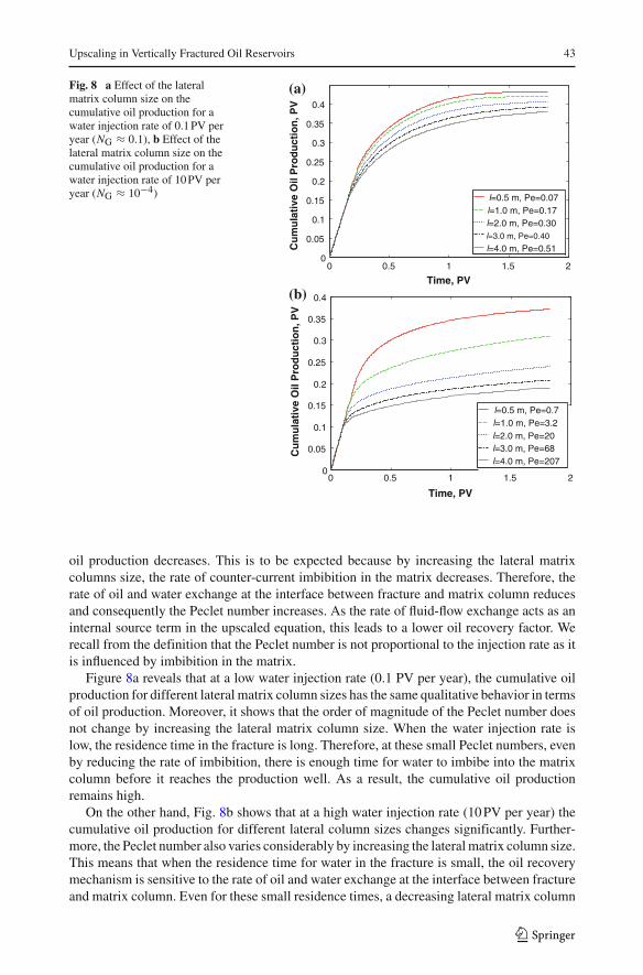
Fig. 8 a Effect of the lateralmatrix column size on thecumulative oil production for awater injection rate of 0.1 PV peryear (NG ≈ 0.1), b Effect of thelateral matrix column size on thecumulative oil production for awater injection rate of 10 PV peryear (NG ≈ 10−4)
0 0.5 1 1.5 20
0.05
0.1
0.15
0.2
0.25
0.3
0.35
0.4
Time, PVC
um
ula
tive
Oil
Pro
du
ctio
n, P
V
l=0.5 m, Pe=0.07l=1.0 m, Pe=0.17l=2.0 m, Pe=0.30l=3.0 m, Pe=0.40
l=4.0 m, Pe=0.51
0 0.5 1 1.5 20
0.05
0.1
0.15
0.2
0.25
0.3
0.35
0.4
Time, PV
Cu
mu
lati
ve O
il P
rod
uct
ion
, PV
l=0.5 m, Pe=0.7l=1.0 m, Pe=3.2l=2.0 m, Pe=20l=3.0 m, Pe=68l=4.0 m, Pe=207
(a)
(b)
oil production decreases. This is to be expected because by increasing the lateral matrixcolumns size, the rate of counter-current imbibition in the matrix decreases. Therefore, therate of oil and water exchange at the interface between fracture and matrix column reducesand consequently the Peclet number increases. As the rate of fluid-flow exchange acts as aninternal source term in the upscaled equation, this leads to a lower oil recovery factor. Werecall from the definition that the Peclet number is not proportional to the injection rate as itis influenced by imbibition in the matrix.
Figure 8a reveals that at a low water injection rate (0.1 PV per year), the cumulative oilproduction for different lateral matrix column sizes has the same qualitative behavior in termsof oil production. Moreover, it shows that the order of magnitude of the Peclet number doesnot change by increasing the lateral matrix column size. When the water injection rate islow, the residence time in the fracture is long. Therefore, at these small Peclet numbers, evenby reducing the rate of imbibition, there is enough time for water to imbibe into the matrixcolumn before it reaches the production well. As a result, the cumulative oil productionremains high.
On the other hand, Fig. 8b shows that at a high water injection rate (10 PV per year) thecumulative oil production for different lateral column sizes changes significantly. Further-more, the Peclet number also varies considerably by increasing the lateral matrix column size.This means that when the residence time for water in the fracture is small, the oil recoverymechanism is sensitive to the rate of oil and water exchange at the interface between fractureand matrix column. Even for these small residence times, a decreasing lateral matrix column
123

44 H. Salimi, H. Bruining
size, which reduces the imbibition time into the matrix column, can lead to a larger delay inwater breakthrough and thus a higher oil production.
6.2 Effect of the Water Injection Rate
Figure 9a and b show the cumulative oil production for a (square) lateral matrix columnsize of 0.5 and 4 m at different water injection rates. Note that we express the (dimension-less) time in terms of cumulative PV water injected. We observe from Fig. 9a and b that asthe water injection rate increases, the corresponding cumulative oil production decreases.When the water injection rate increases, the rate of transport by convection in the fracturealso increases meaning that the residence in the fracture decreases. Consequently, the Pecletnumber becomes larger and the oil recovery factor becomes lower.
As shown in Fig. 9a, the cumulative oil production for a small lateral matrix column size(0.5 m) at different water injection rates has the same qualitative behavior in terms of oilproduction. Figure 9a also reveals that the order of magnitude of the Peclet number does notchange with increasing water injection rate. When the lateral matrix column size is small,the characteristic time of the water imbibition inside the matrix is short, which means that amajor amount of oil in the matrix is depleted by water as soon as water reaches the boundaryof the matrix column because of capillary pressure continuity. Moreover, the characteristicimbibition time is much shorter than the characteristic time of transport by convection inthe fracture. Therefore, even by reducing the residence time in the fracture still the waterimbibition in the matrix is dominant over convection in the fracture. As a result, increasing
Fig. 9 a Effect of the waterinjection rate on the cumulativeoil production for a lateral matrixcolumn size of 0.5 m, b Effect ofthe water injection rate on thecumulative oil production for alateral matrix column size of 4 m
0 0.5 1 1.5 20
0.05
0.1
0.15
0.2
0.25
0.3
0.35
0.4
Time, PV
Cu
mu
lati
ve O
il P
rod
uct
ion
, PV
qw
=0.1 PV/year, Pe=0.07
qw
=1.0 PV/year, Pe=0.30
qw
=10 PV/year, Pe=0.72
0 0.5 1 1.5 20
0.05
0.1
0.15
0.2
0.25
0.3
0.35
0.4
Time, PV
Cu
mu
lati
ve O
il P
rod
uct
ion
, PV
qw
=0.1 PV/year, Pe=0.5
qw
=1.0 PV/year, Pe=5.6
qw
=10 PV/year, Pe=207
(a)
(b)
123
Upscaling in Vertically Fractured Oil Reservoirs 45
the water injection rate does not qualitatively influence the cumulative oil production forsmall lateral matrix column sizes (see Fig. 9a).
However, the cumulative oil production for a large lateral matrix column size (4 m) changessignificantly by varying the water injection rate (Fig. 9b). Moreover, we see from Fig. 9bthat the order of magnitude of the Peclet number also changes, which causes the differentoil production behavior. Here, the time required for water to imbibe into the matrix is longbecause of the large lateral matrix column size (4 m), meaning that the characteristic time ofwater imbibition is long. Furthermore, at a water injection rate of 0.1 PV per year the orderof magnitude of imbibition in the matrix is almost the same as the characteristic time ofconvection in the fracture, i.e., Pe = 0.5. Therefore, at a higher water injection rate (i.e., 1 PVper year and 10 PV per year), the time required for transport by convection in the fracturebecomes much shorter than the time needed for water to imbibe into the matrix column, i.e.,Pe=5.63 and Pe=207. Consequently, this leads to a lower oil recovery factor.
Based on the results shown in Fig. 9a and b, we distinguish two different practical pro-duction scenarios. (1) If a fractured reservoir has a large heterogeneity in matrix column size(fracture spacing), the best strategy to have a high oil recovery factor is to use a low waterinjection rate. (2) If a fractured reservoir contains matrix columns with a relatively smallsize, the best strategy to have a high net present value as well as a relatively high oil recoveryfactor is to use high water injection rates.
6.3 Effect of Gravity
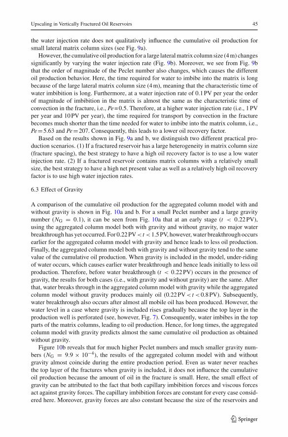
A comparison of the cumulative oil production for the aggregated column model with andwithout gravity is shown in Fig. 10a and b. For a small Peclet number and a large gravitynumber (NG = 0.1), it can be seen from Fig. 10a that at an early stage (t < 0.22 PV),using the aggregated column model both with gravity and without gravity, no major waterbreakthrough has yet occurred. For 0.22 PV< t <1.5 PV, however, water breakthrough occursearlier for the aggregated column model with gravity and hence leads to less oil production.Finally, the aggregated column model both with gravity and without gravity tend to the samevalue of the cumulative oil production. When gravity is included in the model, under-ridingof water occurs, which causes earlier water breakthrough and hence leads initially to less oilproduction. Therefore, before water breakthrough (t < 0.22 PV) occurs in the presence ofgravity, the results for both cases (i.e., with gravity and without gravity) are the same. Afterthat, water breaks through in the aggregated column model with gravity while the aggregatedcolumn model without gravity produces mainly oil (0.22 PV< t <0.8 PV). Subsequently,water breakthrough also occurs after almost all mobile oil has been produced. However, thewater level in a case where gravity is included rises gradually because the top layer in theproduction well is perforated (see, however, Fig. 7). Consequently, water imbibes in the topparts of the matrix columns, leading to oil production. Hence, for long times, the aggregatedcolumn model with gravity predicts almost the same cumulative oil production as obtainedwithout gravity.
Figure 10b reveals that for much higher Peclet numbers and much smaller gravity num-bers (NG = 9.9 × 10⁻⁴), the results of the aggregated column model with and withoutgravity almost coincide during the entire production period. Even as water never reachesthe top layer of the fractures when gravity is included, it does not influence the cumulativeoil production because the amount of oil in the fracture is small. Here, the small effect ofgravity can be attributed to the fact that both capillary imbibition forces and viscous forcesact against gravity forces. The capillary imbibition forces are constant for every case consid-ered here. Moreover, gravity forces are also constant because the size of the reservoirs and
123
46 H. Salimi, H. Bruining
Fig. 10 a Effect of gravity onthe cumulative oil production fora water injection rate of 0.1 PVper year and for a lateral matrixcolumn size of 0.5 m, b Effect ofgravity on the cumulative oilproduction for a water injectionrate of 1 PV per year and for alateral matrix column size of 4 m
0 0.5 1 1.5 20
0.05
0.1
0.15
0.2
0.25
0.3
0.35
0.4
NG=0
0 0.5 1 1.5 20
0.05
0.1
0.15
0.2
0.25
0.3
0.35
NG=9.9×10⁻⁴
NG=0
0 0.5 1 1.5 20
0.05
0.1
0.15
0.2
0.25
0.3
0.35
0.4
Time, PVC
um
ula
tive
Oil
Pro
du
ctio
n, P
V
NG=0.1
NG=0
0 0.5 1 1.5 20
0.05
0.1
0.15
0.2
0.25
0.3
0.35
Time, PV
Cu
mu
lati
ve O
il P
rod
uct
ion
, PV
NG=9.9×10⁻⁴
NG=0
(a)
(b)
the density difference between oil and water are kept constant. The viscous forces changeon the global scale because we vary the rate of water injection as well as the lateral matrixcolumn size. When the Peclet number is small and gravity number is large, the viscous forcesare small and therefore the effects of gravity forces can be observed. On the other hand, ata high Peclet number and very small gravity number, the viscous forces are at least oneorder of magnitude larger than gravity forces. Hence, the viscous forces become dominantand considering gravity forces for these cases does not have a large impact on the cumu-lative oil production. This result is very sensitive to the well outlay and other geometricalconditions.
6.4 Effect of the Fractured Reservoir Topology
Figure 11a and b show the difference in cumulative oil production for the aggregated columnmodel and the sugar cube model. Figure 11a shows the result at a low Peclet number. In thiscase, the sugar cube model and the aggregated column model lead to almost the same result.However, for high Peclet numbers, the sugar cube model (see Fig. 11b) shows a much higherrecovery than the aggregated column model. The reason is that at high Peclet numbers, theimbibition over the full column height is slow and hence oil production from the top of thecolumns is small.
123

Upscaling in Vertically Fractured Oil Reservoirs 47
Fig. 11 a Effect of the fracturedreservoir topology, i.e.,aggregated column versus sugarcube model, for a water injectionrate of 0.1 PV per year and for alateral matrix column size of0.5 m (Pe = 0.07, NG = 0.1),b Effect of the fractured reservoirtopology, i.e., aggregated verticalcolumn versus sugar cube model,for a water injection rate of 10 PVper year and for a lateral matrixcolumn size of 4 m (Pe = 207,NG = 10−4) 0 0.5 1 1.5 2
0
0.05
0.1
0.15
0.2
0.25
0.3
0.35
0.4
Time, PVC
um
ula
tive
Oil
Pro
du
ctio
n, P
V
Aggregated Column
Sugar Cube
0 0.5 1 1.5 20
0.05
0.1
0.15
0.2
0.25
Time, PV
Cu
mu
lati
ve O
il P
rod
uct
ion
, PV
Aggregated ColumnSugar Cube
(a)
(b)
6.5 Comparison Between the Aggregated Column Model and the Effective PermeabilityModel
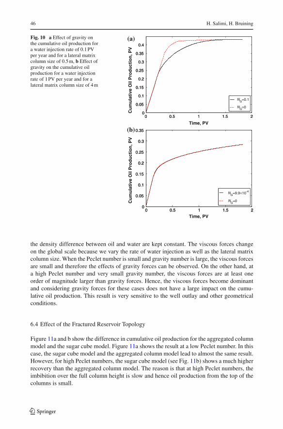
Figure 12a and b show a comparison of the cumulative oil production for the aggregatedcolumn model with the effective permeability model. For a low Peclet number (0.07) (seeFig. 12a), we observe that the aggregated column model predicts a smaller oil productionthan the effective permeability model when more than 0.22 PV of water is injected. Clearlyfor incompressible fluids, the oil production rate and water injection rate before breakthroughare the same, i.e., for t < 0.22 PV. The fracture volume is 0.001 PV, meaning that the oil ismainly produced from the matrix. After t > 1 PV, the results of the aggregated column modeland effective permeability model almost coincide. However, at higher Peclet numbers (e.g.,207 in Fig. 12b), the discrepancy between the aggregated column model and the effectivepermeability model significantly increases, where the aggregated column model predicts anoil recovery factor that is almost two times smaller than the oil recovery factor estimated bythe effective permeability model.
If the Peclet number is small, the rate of oil and water exchange at the interface betweenmatrix column and fracture is fast compared to the rate of convection in the fractures. Inthis case, the residence time in the fracture system is large and most water imbibes into thematrix columns and releases an equal volume of oil to the fracture. Therefore, there is a longperiod when mainly oil is produced at a rate equal to the injection rate (Fig. 12a). As a result,considering a precise rate of fluid exchange at the interface between matrix and fracture is not
123
48 H. Salimi, H. Bruining
Fig. 12 a A comparison of thecumulative oil production for theaggregated column model withthe effective permeability modelfor a water injection rate of0.1 PV per year and for a lateralmatrix column size of 0.5 m(Pe = 0.07, NG = 0.1), b Acomparison of the cumulative oilproduction for the aggregatedcolumn model with the effectivepermeability model for a waterinjection rate of 10 PV per yearand for a lateral matrix columnsize of 4 m (Pe = 207, NG = 10−4)
0 0.5 1 1.5 20
0.05
0.1
0.15
0.2
0.25
0.3
0.35
0.4
Time, PVC
um
ula
tive
Oil
Pro
du
ctio
n, P
V
Aggregated Column
Effective Permeability
0 0.5 1 1.5 20
0.05
0.1
0.15
0.2
0.25
0.3
0.35
0.4
Time, PV
Cu
mu
lati
ve O
il P
rod
uct
ion
, PV
Aggregated Column
Effective Permeability
(a)
(b)
required for the prediction of oil recovery from waterflooded vertically fractured reservoirs.For this reason, one can use the effective permeability model (see Fig. 12a) instead of usingthe aggregated column model. Note that for the effective permeability model, we solved theequations, which correspond to a single conventional porosity model, with porosity equalto the matrix porosity and permeability equal to the effective permeability obtained fromhomogenization. Therefore, the computation time of the effective permeability model is afew hundred times smaller than that of the homogenized model.
On the other hand, if the Peclet number is large, the rate of oil and water exchange atthe interface between the matrix column and the fracture is small compared to the rate ofconvection in the fractures. Consequently, the residence time in the fracture system is small.Therefore, it is expected that the recovery is controlled by the rate of counter-current imbibi-tion from the matrix columns. Hence, one must use the aggregated column model to improveoil recovery predictions from a waterflooded vertically fractured reservoir rather than usingthe effective permeability model. In this case, most of the fractures contain mainly water. Bycapillary continuity, this situation sets the boundary of the matrix columns at the approxi-mately zero capillary pressure or a water saturation of (1 − Sor). As a result of this, there is ashort period in which mainly oil is produced (Fig. 12b), after which oil production becomesvery slow.
123
Upscaling in Vertically Fractured Oil Reservoirs 49
6.6 Comparison Between the Aggregated Column Model and ECLIPSE Simulator (BWRApproach)
Figure 13a–c show a comparison of the cumulative oil and water production for the aggregatedcolumn model with the ECLIPSE simulator. For a small Peclet number (0.07, Fig. 13a), themodel and the simulator show the same breakthrough time, i.e., t = 0.22 PV. Subsequently,at 0.22 PV< t <0.67 PV, the ECLIPSE simulator predicts a higher oil production rate thanthe aggregated column model as illustrated by the fact that the slope of cumulative oil produc-tion curve for the ECLIPSE simulator at this stage is steeper than the slope of the cumulativeoil production curve for the aggregated column model. Finally, both the aggregated columnmodel and ECLIPSE results tend to different values of oil production. The discrepancy inFig. 13a between the aggregated column model and ECLIPSE is due to large gravity effects,which requires an accurate representation of the fracture–matrix interaction. For a slightlyhigher Peclet number (Fig. 13b), we see that the cumulative oil production for the aggregatedcolumn model and the ECLIPSE simulator almost coincide. Therefore, in this condition, theaggregated column model can be replaced by the BWR approach without appreciable lossof accuracy.
The results at still higher Peclet numbers are shown in Fig. 13c. In this case, the aggre-gated column model predicts a higher oil production at an early stage than the ECLIPSEsimulator because of fast depletion of oil from the part of the matrix column adjacent to thefracture resulting from continuity of capillary pressure. Afterwards, the predicted rate of oilproduction of ECLIPSE exceeds the rate of oil production of the aggregated column model,and gradually the cumulative oil production from the ECLIPSE simulator reaches the valueof the cumulative oil production for the aggregated column model.
The most important reason for the discrepancy between the aggregated column modeland ECLIPSE model is the difference between the BWR transfer function and the fluid-flow exchange term based on homogenization. The second most important reason is thatthree-dimensional matrix-block subgridding to the best of our knowledge is not availablein the ECLIPSE simulator. The third most important reason is that there is no option in theECLIPSE simulator for the aggregated column topology. We observe that most of the dis-crepancy between the aggregated column model and ECLIPSE simulator happens at higherand lower Peclet numbers. In these cases, accurate fluid-flow exchange terms are necessaryfor the accurate prediction of oil recovery because the oil recovery is controlled by the rate ofimbibition for high Peclet numbers and by gravity for high gravity numbers. Consequently,satisfying the continuity of the capillary pressure has a significant effect on the cumulativeoil production.
Figures 12a and 13b show a small difference between the aggregated column model andthe effective permeability model and ECLIPSE. We explain this observation as follows. Whenthe Peclet number is small but not so small that gravity starts to dominate (see Fig. 13a),the rate of fluid transport in the fracture controls the oil recovery mechanism. Therefore, inthis regime, considering an accurate rate of fluid exchange at the interface between matrixand fracture is not required for the prediction of oil recovery from waterflooded verticallyfractured reservoirs. For this reason, one can use either the effective permeability model orthe BWR approach (see Fig. 13b) instead of using the aggregated column model. Hence,when the Peclet number is small, but not so small that gravity starts to dominate, we can useeither the effective permeability model or the BWR approach (Fig. 13b), instead of usingthe aggregated column model. Note that the effective permeability model does not have anexchange term because it is a single-porosity model. Therefore, it can be easily implementedand uses little computational time compared to the other two models. On the other hand,
123

50 H. Salimi, H. Bruining
Fig. 13 a A comparison of thecumulative oil productionbetween the aggregated columnmodel and ECLIPSE simulator(BWR approach) for a waterinjection rate of 0.1 PV per yearand for a lateral matrix columnsize of 0.5 m (Pe = 0.07,NG = 0.1), b A comparison of thecumulative oil productionbetween the aggregated columnmodel and ECLIPSE simulator(BWR approach) for a waterinjection rate of 1 PV per year andfor a lateral matrix column size of1 m (Pe = 0.45, NG = 0.005), c Acomparison of the cumulative oilproduction between theaggregated column model andECLIPSE simulator (BWRapproach) for a water injectionrate of 1 PV per year and for alateral matrix column size of 2 m(Pe = 1.01, NG = 0.002)
0 0.5 1 1.5 20
0.1
0.2
0.3
0.4
0.5
Time, PVC
um
ula
tive
Oil
Pro
du
ctio
n, P
V
Aggregated ColumnECLIPSE
0 0.5 1 1.5 20
0.05
0.1
0.15
0.2
0.25
0.3
0.35
0.4
Time, PV
Cu
mu
lati
ve O
il P
rod
uct
ion
, PV
Aggregated Column
ECLIPSE
(a)
(b)
(c)
0 0.5 1 1.5 20
0.05
0.1
0.15
0.2
0.25
0.3
0.35
0.4
Time, PV
Cu
mu
lati
ve O
il P
rod
uct
ion
, PV
Aggregated ColumnECLIPSE
there is a critical Peclet number marking the boundary between the two regimes. If the Pecletnumber is large (as in Figs. 12b and 13c), there is a large difference between the homogenizedmodel and either the effective permeability model or the BWR approach. In this regime, theoil recovery mechanism is controlled by the rate of imbibition from the matrix columns. Inthis case, the exchange rate between matrix and fracture is better described by the physicallybased homogenization approach than by the semi-empirical BWR approach. Therefore, wemust use the aggregated column model when the Peclet number is large.
123
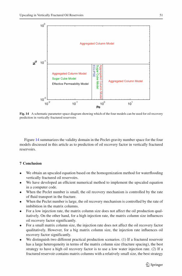
Upscaling in Vertically Fractured Oil Reservoirs 51
10-2
10-1
100
101
10-2
10-1
100
Pe
NG
Aggregated C
olumn M
odel S
ugar Cube M
odel E
CLIP
SE
Aggregated Column Model
Aggregated Column Model
Aggregated Column Model
Sugar Cube Model
Effective Permeability Model
Fig. 14 A schematic parameter-space diagram showing which of the four models can be used for oil recoveryprediction in vertically fractured reservoirs
Figure 14 summarizes the validity domain in the Peclet-gravity number space for the fourmodels discussed in this article as to prediction of oil recovery factor in vertically fracturedreservoirs.
7 Conclusion
• We obtain an upscaled equation based on the homogenization method for waterfloodingvertically fractured oil reservoirs.
• We have developed an efficient numerical method to implement the upscaled equationin a computer code.
• When the Peclet number is small, the oil recovery mechanism is controlled by the rateof fluid transport in the fracture.
• When the Peclet number is large, the oil recovery mechanism is controlled by the rate ofimbibition in the matrix columns.
• For a low injection rate, the matrix column size does not affect the oil production qual-itatively. On the other hand, for a high injection rate, the matrix column size influencesoil recovery factor significantly.
• For a small matrix column size, the injection rate does not affect the oil recovery factorqualitatively. However, for a big matrix column size, the injection rate influences oilrecovery factor significantly.
• We distinguish two different practical production scenarios. (1) If a fractured reservoirhas a large heterogeneity in terms of the matrix column size (fracture spacing), the beststrategy to have a high oil recovery factor is to use a low water injection rate. (2) If afractured reservoir contains matrix columns with a relatively small size, the best strategy
123

52 H. Salimi, H. Bruining
to have a high net present value as well as a relatively high oil recovery factor is to usea high water injection rate.
• At low gravity numbers, gravity does not affect oil production. On the other hand, atintermediate and large gravity numbers considering gravity is necessary.
• The results show that in spite of the difference between the fluid-flow exchange termin the homogenized sugar cube model and the fluid-flow exchange term in the homoge-nized aggregated column model, the cumulative oil productions predicted by these twomodels are almost the same at low Peclet numbers. However, at large Peclet numbers,the reservoir topology needs to be considered precisely.
• When the Peclet number is low, the vertically fractured reservoir behaves like a highlyheterogeneous single-porosity reservoir. Therefore, the effective permeability model canreplace the aggregated column model without appreciable loss of accuracy. The advan-tage of the effective permeability model is again that its computations are not time-con-suming as opposed to the aggregated column model.
• At a low Peclet number, gravity starts dominating; therefore, the aggregated columnmodel cannot be replaced by the BWR approach because in the vertically fractured res-ervoir (aggregated column) gravity plays an important role. However, at intermediatePeclet numbers, one can use the BWR model to predict oil recovery factor from water-flooded vertically fractured reservoirs without loss of accuracy. On the other hand, athigh Peclet numbers the aggregated column model, which represents the physics of theproblem better than the BWR approach, should be used.
• In view of homogenization’s physical basis, we assert that improved fracture model-ing can be achieved using the upscaled aggregated column model. Figure 14 presents a“phase diagram” that can be used as an indication for the appropriate model or indicateswhen traditional modeling is adequate.
Acknowledgments We thank Statoil-Hydro for supporting our research on oil recovery from fractured reser-voirs. We also thank Sharif University of Technology for their steady collaboration. We acknowledge MaryamNamdar Zanganeh, William R. Rossen, Stefan M. Luthi, and Giovanni Bertotti for many useful discussionsand comments. We also acknowledge SPE for granting the Nico van Wingen Memorial Graduate Fellowshipin Petroleum Engineering to Hamidreza Salimi.
Open Access This article is distributed under the terms of the Creative Commons Attribution Noncommer-cial License which permits any noncommercial use, distribution, and reproduction in any medium, providedthe original author(s) and source are credited.
References
Aguilera, R.: Geological aspects of naturally fractured reservoirs. Lead. Age 17(12), 1667–1670 (1998)AI-Harbi, M., Cheng, H., He, Z., Datta-Gupta, A.: Streamline-based production data integration in naturally
fractured reservoirs. Soc. Petrol. Eng. J. 10(4), 426–439 (2005)Al-Huthali, A., Datta-Gupta, A.: Streamline simulation of counter-current imbibition in naturally fractured
reservoirs. J. Petrol. Sci. Eng. 43(3–4), 271–300 (2004)Arbogast, T.: Gravitational forces in dual-porosity systems: I. Model derivation by homogenization. Transp.
Porous Media 13(2), 179–203 (1993a)Arbogast, T.: Gravitational Forces in Dual-Porosity Systems: II. Computational Validation of the Homogenized
Model. Transp. Porous Media 13(2), 205–220 (1993b)Arbogast, T. : Computational aspects of dual-porosity models. In: Hornung, U. (ed.) Homogenization and
Porous Media, Interdisciplinary Applied Mathematics, 6th edn, pp. 203–223. Springer, New York (1997)Arbogast, T., Douglas, J. Jr., Hornung, U.: Derivation of the double porosity model of single phase flow via
homogenization theory. SIAM J. Math. Anal. 21(4), 823–836 (1990)
123

Upscaling in Vertically Fractured Oil Reservoirs 53
Barenblatt, G.I., Zheltov, I.P., Kochina, I.N.: Basic concepts in the theory of seepage of homogenous liquidsin fissured rocks. J. Appl. Math. Mech. 24(5), 852–864 (1960)
Berkowitz, B., Kosakowski, G., Margolin, G., Scher, H.: Application of continuous time random walk theoryto tracer test measurements in fractured and heterogeneous porous media. Ground Water 39(4), 593–604 (2001)
Chen, Z.: Homogenization and simulation for compositional flow in naturally fractured reservoirs. J. Math.Anal. Appl. 326(1), 12–32 (2007)
De Dreuzy, J.-R., Davy, P., Bour, O.: Hydraulic properties of two-dimensional random fracture networksfollowing power law distributions of length and aperture. Water Resour. Res. 38(12), 121–129 (2002)
De Dreuzy, J.-R., Darcel, C., Davy, P., Bour, O.: Influence of spatial correlation of fracture centers on thepermeability of two-dimensional fracture networks following a power law length distribution. WaterResour. Res. 40(1), W015021–W0150211 (2004)
Di Donato, G., Blunt, M.: Streamline-based dual-porosity simulation of reactive transport and flow in fracturedreservoirs. Water Resour. Res. 40(4), W042031–W0420312 (2004)
Douglas, J. Jr., Hensley, J.L., Arbogast, T.: A dual-porosity model for waterflooding in naturally fracturedreservoirs. Comput. Methods Appl. Mech. Eng. 87(2–3), 157–174 (1991)
Douglas, J. Jr., Arbogast, T., Paes-Leme, P.J., Hensley, J.L., Hunes, N.P.: Immiscible displacement in verticalfractured reservoirs. Transp. Porous Media 12(1), 73–106 (1993)
Firoozabadi, A.: Recovery mechanisms in fractured reservoirs and field performance. J. Can. Petrol. Tech-nol. 39(11), 13–17 (2000)
Hornung, U.: Homogenization and Porous Media, Interdisciplinary Applied Mathematics, 6th edn.Springer, New York (1997)
Hoteit, H., Firoozabadi, A.: Compositional modeling of discrete-fractured media without transfer functionsby the discontinuous galerkin and mixed methods. Soc. Petrol. Eng. J. 11(3), 341–352 (2006)
Kazemi, H., Seth, M.S., Thomas, G.W.: The interpretation of interference tests in naturally fractured reservoirswith uniform fracture distribution. Soc. Petrol. Eng. J. 9(4), 463–472 (1969)
Kazemi, H., Gilman, J.R., Elasharkawy, A.M.: Analytical and numerical solution of oil recovery from fracturedreservoirs with empirical transfer functions. Soc. Petrol. Eng. Reserv. Eng. 7(2), 219–227 (1992)
Lewandowska, J., Szymkiewicz, A., Auriault, J.L.: Upscaling of Richards’ equation for soils containing highlyconductive inclusions. Adv. Water Resour. 28, 1159–1170 (2005)
Margolin, G., Berkowitz, B., Scher, H.: Structure, flow, and generalized conductivity scaling in fracture net-works. Water Resour. Res. 34(9), 2103–2121 (1998)
Nelson, R.A.: Geologic Analysis of Naturally Fractured Reservoirs. Gulf Publishing Co., Houston, TX (1985)Park, Y.-J., de Dreuzy, J.-R., Lee, K.-K., Berkowitz, B.: Transport and intersection mixing in random fracture
networks with power law length distributions. Water Resour. Res. 37(10), 2493–2501 (2001)Pooladi-Darvish, M., Firoozabadi, A.: Cocurrent and countercurrent imbibition in a water-wet matrix
block. Soc. Petrol. Eng. J. 5(1), 3–11 (2000)Salimi, H., Bruining, J.: Improved prediction of oil recovery from waterflooded fractured reservoirs using
homogenization. Soc. Petrol. Eng. Reserv. Eng. Eval. (2009). doi:10.2118/115361-PASarma, P., Aziz, K.: New transfer function for simulation of naturally fractured reservoirs with dual-porosity
models. Soc. Petrol. Eng. J. 11(3), 328–340 (2006)Shook, M., Li, D., Lake, L.W.: Scaling immiscible flow through permeable media by inspectional analysis. In
Situ 16(4), 311–349 (1992)Sonier, F., Souillard, P., Blaskovich, F.T. : Numerical simulation of naturally fractured reservoirs. Soc. Petrol.
Eng. Reserv. Eng. 3(4), 1114–1122 (1988)Tartar, L.: Incompressible fluid flow in a porous medium—convergence of the homogenization process. In:
Sanchez-Palencia, E. (ed.) Lecture Notes in Physics, vol. 127, pp. 368–377. Springer, New York (1980)Van Duijn, C.J., Molenaar, J., Neef, M.J.: The effect of capillary forces on immiscible two-phase flow in
heterogeneous porous media. Transp. Porous Media 21(1), 71–93 (1995)Van Duijn, C.J., Mikelic, A., Pop, I.S.: Effective equations for two-phase flow with trapping on the micro
scale. SIAM J. Appl. Math. 62(5), 1531–1562 (2002)Van Duijn, C.J., Mikelic, A., Pop, I.S., Rosier, C.: Effective dispersion equations for reactive flows with
dominant Péclet and Damkohler numbers. Adv. Chem. Eng. 34, 1–45 (2008)Warren, J.E., Root, P.J.: The behavior of naturally fractured reservoirs. Soc. Petrol. Eng. J. 3(3), 245–255 (1963)Wu, Y.S., Pan, L., Pruess, K.: A physically based approach for modeling multiphase fracture–matrix interaction
in fractured porous media. Adv. Water Resour. 27, 875–887 (2004)Yortsos, Y.C.: A theoretical analysis of vertical flow equilibrium. Paper SPE 22612 presented at the SPE annual
technical conference and exhibition, Dallas, TX, 6–9 October 1991. doi:10.2118/22612-MS
123