unstructured tetrahedral mesh generation...

ISSN 0965�5425, Computational Mathematics and Mathematical Physics, 2010, Vol. 50, No. 1, pp. 139–156. © Pleiades Publishing, Ltd., 2010.Original Russian Text © A.A. Danilov, 2010, published in Zhurnal Vychislitel’noi Matematiki i Matematicheskoi Fiziki, 2010, Vol. 50, No. 1, pp. 146–163.

139

INTRODUCTION

Unstructured tetrahedral meshes are widely used in mathematical modelling due to their simplicityand ability to represent complex domains. A tetrahedral mesh is called conformal, if each its two tetrahe�dra have one common vertex, one entire common edge, or one entire common face, or do not have anycommon points. The similar definition applies to conformal triangulations. Mesh conformity is an impor�tant and desirable property. In this paper we use a notion “triangulation” for both tetrahedral and trian�gular meshes, if it does not lead to an ambiguity.

Mesh generation process consists of two stages: surface meshing and volume meshing. At the first stagewe construct a surface conformal triangular mesh. The surface mesh can be produced in several differentways. At the second stage we mesh the volume inside the domain into tetrahedra while preserving givensurface triangular mesh on the boundary.

In 2D case, we can always construct a boundary conforming triangulation without insertion of newpoints inside a given polygon. In 3D case, for some polyhedra no triangulation is possible without inser�tion of additional points. An example of such polyhedron is shown in Fig. 1—Schönhardt prism [1].Insertion of just one point inside the convex polyhedron can solve the problem as shown by Joe [2].George [3] has shown the existence of a tetrahedral boundary conforming mesh for an arbitrary polyhe�dron with possible addition of several internal points. However, robust construction of a conformal tetra�hedral mesh with fixed boundary triangulation is a challenging problem.

There exist two main approaches for tetrahedral mesh generation: methods based on Delaunay trian�gulations (DT), and advancing front technique (AFT). The Delaunay triangulation approach does notguarantee the boundary conformity. Several techniques are proposed to match the boundary: local meshtransformations [4], mesh refinement [5], and constrained Delaunay triangulations (CDT) [6]. On theother hand, the advancing front technique does not have issues with boundary recovery since it starts fromthe given surface mesh [7]. However, AFT methods have difficulties in successfully closing up their fronts.Combining both AFT and DT ideas, one proposed hybrid methods [8]. Our volume mesh generationmethod is a combination of a conventional AFT method and a DT based fallback method.

In this paper we present several methods for defining and meshing domain boundaries, and a combi�nation of the two methods for volume meshing. In Section 1 we propose four methods for boundary mesh�ing using analytical boundary parameterization, interface with CAD systems, surface mesh refinement,and solid constructive geometry (SCG). In Section 2 we discuss a classical AFT method for volume mesh�ing. This method does not guarantee us a successful meshing. That is why we use a fallback method basedon DT and boundary faces recovery. A simplified version of this George’s method [9] is discussed in Sec�

Unstructured Tetrahedral Mesh Generation Technology1

A. A. DanilovInstitute of Numerical Mathematics of the Russian Academy of Sciences, ul. Gubkina, 8, Moscow, 119333 Russia

e�mail: [email protected] November 17, 2008

Abstract—We present a robust unstructured tetrahedral mesh generation technology. This technologyis a combination of boundary discretization methods, an advancing front technique and a Delaunay�based mesh generation technique. For boundary mesh generation we propose four differentapproaches using analytical boundary parameterization, interface with CAD systems, surface meshrefinement, and constructive solid geometry. These methods allow us to build a flexible grid generationtechnology with a user friendly interface.

DOI: 10.1134/S0965542510010124

Key words: advancing front technique, constrained Delaunay triangulations mesh generation.

1The article is published in the original.

140

COMPUTATIONAL MATHEMATICS AND MATHEMATICAL PHYSICS Vol. 50 No. 1 2010

DANILOV

tion 3. In Section 4 we briefly discuss robustness issues of volume meshing. In Section 5 we provide severalapplication examples.

The presented technology is implemented as a part of Ani3D package [10], the successor of Ani2Dpackage [11]. Both packages provide tools for unstructured mesh generation, anisotropic metric�basedadaptation, finite element discretization, and linear system solving. These packages are publicly available.In each section we pay special attention to our actual Ani3D implementations of discussed methods.Some technical information will be provided for our AFT method as well.

1. SURFACE MESH GENERATION

In this section we will discuss several methods for defining and meshing the surface, which representsa domain boundary. The main idea is to split the surface into several pieces sharing common boundarylines. Though in general these lines may be curves, for simplicity we just call them lines. Then, assumingthat we have discretization of the boundary lines, we can use an advancing front method on each piece.Since all pieces of the surface have the same discretization on the boundary lines, the resulting surfacemesh will be conformal.

Keeping this idea in mind we propose four different approaches for surface meshing. They are basedon:

(1) analytical boundary parameterization;(2) interface with CAD systems based on a boundary representation (BREP) model;(3) surface mesh refinement and coarsening; (4) surface meshing of solid constructive geometry models.Analytical boundary parameterization method is used for simple domains: spheres, boxes, cylinders,

and polyhedra with planar faces. Complex domains like a union or an intersection of several simple prim�itives can be processed with solid constructive geometry approach. More complex domains designed inCAD systems can be meshed with a help of an interface between a CAD system and a mesh generator. Adomain boundary can also be defined by a surface mesh produced by an unattainable CAD system. Sincethe resulting volume mesh quality strongly depends on surface mesh quality, an additional surface meshrefining may be required. On the other hand, too fine surface mesh can produce unnecessarily fine volumemesh, in this case an additional surface coarsening can be performed. These preprocessing tools allow usto adopt and use many available surface meshes.

1.1. Analytical Boundary Parameterization

This is a straightforward application of the general idea discussed above. We split the boundary surfaceof the domain into several pieces Σi called patches. Each of them is parameterized separately by a smoothfunction:

A boundary line Γk between two adjacent patches is also parameterized:

Σi x y z, ,( ) x y z, ,( ) fi u v,( ) u v,( ) Ωi �2

⊂∈,={ }.=

Γk x y z, ,( ) x y z, ,( ) gk t( ) t tk0

tk1

,[ ]∈,={ }.=

12

3

45

6

12

3

45

6

Fig. 1. The Schönhardt prism: convex prism and twisted non�convex prism (the hidden edge is 1–5). No conformal tri�angulation is possible without insertion of additional points.


UNSTRUCTURED TETRAHEDRAL MESH GENERATION TECHNOLOGY 141

We also need the mappings (uik, vik) from a boundary line parameterization space to the surface parame�terization space for each patch:

In general, for some functions fi, gk these mappings uik, vik may appear to be analytically non�computable.Thus this method is applicable only for very simple domains.

Alternatively, the user can define a separate boundary line parameterization in (u, v) space for eachseparate patch. Let us consider a patch i parameterized by function fi(u, v). We can represent its boundary

line Γk by a curve in (u, v) space. For instance, if we use the mapping u (u, vik(u)), then in �3 the

boundary line will be parameterized as follows:

These parameterizations of Γk will be different for different patches, but they should represent the samegeometry. The latter approach is the one used in Ani3D package for analytical boundary representation.

In order to create a surface mesh for each patch, boundary lines are discretized first. Let us consider aparameterized boundary line:

We create new points on the line:

Parameter points τi ∈ [u0, u1] are selected by an edge subdivision method according to desired distancebetween points Pi.

Once the boundary discretization on the patch is constructed, we use the 2D AFT method to constructa triangular mesh. In this AFT method we work simultaneously in both (u, v) space and (x, y, z) space.The 2D AFT method will be briefly discussed in Section 2.

This method for surface meshing is a general approach. Parameterization functions may be compli�cated for complex surfaces and especially for their intersection lines. Thus this method is applicable inrather simple cases. An example of initial geometry and generated surface mesh is presented in Fig. 2.

1.2. Interface with CAD System

In many cases a domain can be modeled in a CAD system. Most of CAD kernels use a boundary rep�resentation (BREP) model as an internal model representation. In this model four types of topologicalentities are used: vertices, edges, faces, and volumes. Beside this, the BREP model provides adjacencyrelationships between the entities. Each face and each edge have their own parameterization stored by theCAD kernel. For instance, NURBS are widely used in CAD kernels for surface parameterizations.

The topology model and the parameterizations of lines and surfaces provide all necessary data to applyanalytical boundary parameterization method. Several ways may be used to obtain this data. One optionis to implement a special file reader. This reader loads all data from CAD file, and works with NURBS orother types of used parameterizations. Another option is to query all data directly from the CAD kernel,or through a special abstracting interface layer between the CAD kernel and the AFT generator. The sec�

gk t( ) fi uik t( ) vik t( ),( ), t tk0

tk1

,[ ].∈=

Γk x y z, ,( ) x y z, ,( ) fi u vik u( ),( ) u uk0

uk1

,[ ]∈,={ }.=

x y z, ,( ) g u( ) f u v u( ),( ), u u0 u1,[ ].∈= =

Pi g τi( ), i 0 1 … n., , ,= =

(a) (b)

Fig. 2. Analytical boundary parameterization: (a) boundary lines discretization; (b) surface mesh.

142


DANILOV

ond option is more appealing, since there is no need to implement different file format readers and differ�ent parameterization types.

In Ani3D package we used the interface layer approach on the basis of a common functional interface.The layer can be easily used to switch between different CAD kernels without the need of rewriting themesh generator itself. The Common Geometry Module (CGM) [12] is chosen as an abstracting layer: itintegrates with OpenCASCADE [13], ACIS, and Pro/Engineer geometry kernels. Interfacing a CAD sys�tem with a mesh generator is mainly a technical task. An example of a CAD model and a surface mesh areillustrated in Fig. 3.

1.3. Surface Mesh Refinement and Coarsening

In some cases the domain already has a boundary mesh. However, the surface mesh may be ill�shaped,like meshes exported from CAD systems. In this case constructing a volume mesh inside the domain willbe hampered or will result in an ill�shaped volume mesh. In Ani3D package we introduced a new tech�nique for surface mesh modification [14]. The basic idea is to split the surface into several nearly flat poly�gons, and remesh them. In order to construct a nearly flat polygon, we define a criterion, and use it to addtriangles to the polygon. We use the following criterion. Triangle T nearly lies in plane P, if an anglebetween the normals to the triangle T and to the plane P is small enough, and a distance from the triangleT to the plane P is also small. The user can control the value of admissible deviation.

After the surface is split into several nearly flat polygons, we create a new boundary discretization ofthese polygons. This boundary discretization should be consistent across different polygons. To achievethis, we compute a mesh size function in the vertices and interpolate it on the edges. According to thismetric we discretize the edges, thus ensuring consistency across polygons.

For each polygon we construct a new triangular mesh. To this end, we make a projection of the polygonand its new boundary discretization on a plane, construct a new triangular mesh using planar AFT startingfrom the new boundary discretization, and project the new mesh from the plane back to the surface. Sincethe original polygon was nearly flat, a surface distortion caused by the projection will be insignificant.

At the end of this process a new conformal surface triangulation is created. The detailed algorithm ispresented in Algorithm 1.

Algorithm 1. Surface mesh modification

for all vertices Vi, do

Compute a mesh size function hi = h(Vi) based on the size of surrounding triangles

in the initial surface meshend forwhile there are unexamined triangles do

Pick an arbitrary triangle T0 from the initial mesh

Construct a plane P containing triangle T0

Initialize a new polygon M = {T0}

for all neighboring triangles Tk do

if Tk nearly lies in P then

(a) (b)

Fig. 3. Interface with CAD system: (a) model in CAD system; (b) surface mesh.



Add triangle Tk to the set M

end ifend forfor all boundary edges Ej of polygon M do

Linearly interpolate the mesh size values hi on the edge

Create an edge discretization based on the interpolated metricend forProject polygon M and its new boundary discretization on the plane PConstruct a new triangular mesh using planar AFTProject a new mesh from P back to MDiscard M from initial mesh

end whileThis method is useful for remeshing an ill�shaped surface mesh exported from CAD system into a more

regular surface mesh. This technique may also be used for coarsening an initial fine mesh. To this end, weuse a moderate admissible deviation for triangle normals. In this case polyregions will have much moretriangles. Then, for each polyregion we can construct a new coarse triangular mesh resulting in a new morecoarse surface mesh. Both examples of surface refinement and coarsening are presented in Figs. 4 and 5respectively.

1.4. Solid Constructive Geometry

Some domains are rather complex for analytical representation, but still simple enough for using hugeCAD systems. Important examples are intersections and unions of simple objects (primitives) like boxes,spheres, cylinders. This type of geometry representation is frequently called solid constructive geometry(SCG). The idea of implementing boundary meshing for SCG models is as follows [15]. For a simpleprimitive a surface mesh is generated using an analytical parameterization. Two surface meshes represent�ing two primitives are intersected to provide a new surface mesh for a union or an intersection of the twoprimitives. The new object is then treated as another primitive.

(a) (b)

Fig. 4. Surface mesh refinement: (a) initial surface mesh; (b) refined surface mesh.

(a) (b)

Fig. 5. Surface mesh coarsening: (a) initial surface mesh; (b) coarsened surface mesh.

144


DANILOV

The mesh intersection is performed in three stages.At the first stage we intersect two surface meshes, and construct a polyline of the intersection. This line

splits each surface mesh into three parts: two surface parts and an intersection band. Depending on a log�ical operation used (union, intersection or difference), one of two parts will lie either inside or outside theresulting object. The other surface part will lie on the surface of the object.

At the second stage we remove triangles from the intersection band, as well as triangles which do notlie on the new surface.

At the third stage we remesh the band near the intersection polyline ensuring conformity of the finalmesh, and perform local mesh optimizations in order to improve the mesh quality near the intersectionline.

The detailed algorithm is presented in Algorithm 2.

Algorithm 2. Surface mesh intersection

Intersect two meshes: Γ = M1 ∩ M2

for each mesh Mi do

for each triangle T doDetermine if T intersects Γ, or T lies inside the new surface, of T lies outside it

end for

Split Mi into three parts: triangles forming intersection band, triangles

lying inside the new surface, and triangles lying outside it

end for

Replace mesh parts with a new conformal mesh Mband

Unite the new intersection band mesh Mband with two other surface parts

An example of this approach application is shown in Fig. 6. In Ani3D package the user may create anduse his own arbitrary primitives by providing their boundary meshes. In particular, user may crop an inter�esting region from an already obtained surface mesh by intersecting it with a rectangular box.

2. ADVANCING FRONT TECHNIQUE

In this section we discuss an advancing front technique which is used to construct a volume mesh insidea bounded domain. We define the front as a set of oriented triangular faces forming a closed conformalsurface mesh. The idea of AFT is to exhaust this front by advancing it inside the domain and constructingnew tetrahedra. The front actually divides the domain into two parts: already meshed one and the remain�ing part. At each step a new tetrahedron is constructed and the front is advanced. If the front is void, thenthe mesh is fully constructed, and AFT algorithm terminates.

Let us discuss one step of this method. In Fig. 7 we show main substeps in 2D case.

Miband

Miin

Miout

Miband

Miin

(a) (b)

Fig. 6. Solid constructive geometry: (a) two surface meshes; (b) conformal surface mesh.



We start by selecting an unvisited face with the smallest area from the current front, we call it the cur�rent face. We construct a new tetrahedron based on the current face, i.e. we construct a normal vector fromthe center of the face, and place the fourth vertex on its end (see Fig. 7b). The length of the vector is basedeither on a user�defined mesh size, or on a product of a current face size and a user�defined stretching fac�tor k. In the latter case, AFT method will result in a quasi�uniform mesh with k = 1, and it will result inan automatic mesh coarsening away from the boundary with k > 1. Automatic mesh coarsening will be dis�cussed in the next subsection.

We are going to find a suitable tetrahedron and add it to the mesh. A tetrahedron is assumed to be suit�able if it does not intersect the front, does not degenerate, and does meet other user requirements. We startfrom just constructed tentative tetrahedra and check if it is suitable. If not, we iterate through the front ver�tices and try to use them as the fourth vertex of the tentative tetrahedron, until a suitable tetrahedron isfound (see Fig. 7c).

If no tetrahedron was found, then we skip and mark the current face as visited. These marks will becleared later and faces will be revisited. If a suitable tetrahedron was found, then we add it to the mesh andupdate the front: we delete the current face, and either delete from the front, or add to the front each ofthe other three faces (see Fig. 7d).

We repeat the whole process until the front is void or all faces are marked as visited. In the last case weclear the marks and restart the whole process. If the front can not be advanced further, then anothermethod should be used to mesh the remaining part of the domain. At the end we can perform a simplemesh smoothing in order to improve mesh quality.

The formal algorithm of AFT method is presented in Algorithm 3.The similar technique is used in 2D case. In planar 2D case the mesh can always be constructed using

just AFT method. The 2D case on a parameterized surface differs from

Algorithm 3. Advancing front technique

while front is not void doPick the smallest face F = �ABC from the current front Γif all faces are already visited then

Stop AFTend if

(a) (c)

(b) (d)

Fig. 7. One step of AFT method in 2D case: (a) current front; (b) constructed triangle; (c) suitable triangle; (d) updatedfront.

146


DANILOV

Determine the desired mesh size near F

Compute a tentative position for the new point P

Locate front triangles ΓB and front points VB in a vicinity of P

if there are front points near P then

Set D as the nearest front point

else

Set D = P

end if

while tetrahedron ABCD is tangled, or is degenerated, or intersects ΓB do

Pick another candidate D from VB,

if there are no more candidates then

Mark F as visited, and goto 2

end if

end while

Add tetrahedron ABCD to the mesh

for each oriented face Fi of ABCD do

if inverted face is in the front then

Remove from the front

else

Add to the front

end if

end for

end while

The similar technique is used in 2D case. In planar 2D case the mesh can always be constructed usingjust AFT method. The 2D case on a parameterized surface differs from the planar 2D case in that part,where a new point is constructed to form a triangle. A new point is searched in (u, v) space in such a waythat the resulting triangle will be isosceles in (x, y, z) space. An intersection between a new tentative trian�gle and the existing front is checked in (x, y, z) space.

2.1. Finiteness of AFT Algorithm

In this subsection we will go into the details of AFT method used in Ani3D package. Let us first con�sider the case, when an automatic mesh coarsening is used. In our AFT method we follow the next rule.Addition of a new vertex should not decrease the minimal pairwise distance ρ between vertices in themesh. On a regular AFT step we consider the front triangle ABC, where a, b, c are its edge lengths. Let Mbe a barycenter of the triangle. We construct a normal to plane ABC going through point M, and positionthe point D on its end. Distance MD = h is chosen automatically according to coarsening factor k. We usethe following formula for h:

According to mean inequality, h � , with equality being achieved only when a = b = c.

Keeping in mind that k � 1, we get h2 � . Now we consider the length of AD, AD2 =

Fi*

Fi*

Fi*

h a3

b3

c3

+ +3

��3 k 23�� .=

a2

b2

c2

+ +3

��k 23��

2a2

2b2

2c2

+ +9

��



AM2 + MD2. Length of AM is computed by median length formula: AM = . We get

AM2 = , and finally

Since triangle side lengths a, b, c are not less than ρ, then AD � ρ as well. In case of k = 1 and equilateraltriangle ABC we get AD = a = b = c. The same applies for other edges BD and CD. Thereby the fourth pointD will be distanced enough from the triangle.

Additionally, we will check that there are no other front points in ρ�vicinity of the fourth point D. Ifsuch points exist, then the point D is not considered, and the search is started from the nearest front point.Following these rules we can guarantee that the minimal pairwise distance between points is not less thanρ. In this case the total number of vertices will be bounded above, and the total number of tetrahedra willbe bounded above as well.

The case, when the value of h is defined according to the user�defined mesh size function F(x), is sim�ilar. If F(x) > F0 > 0 in the whole domain, then the minimal pairwise point distance is limited bellow, andthe number of tetrahedra is limited above. If F(x) may be arbitrary small, then AFT algorithm may end upin infinite refinement loop.

Summing up, if automatic mesh coarsening is used, or if user�defined mesh size function is isolatedfrom zero, then the total number of points and tetrahedra is bounded above, thus the number of AFT iter�ations is also bounded above.

2.2. Complexity of AFT Algorithm

In order to analyze the complexity of the proposed algorithm, we focus on the following operationswith the front:

(1) add a new face into the front;(2) delete an existing face from the front;(3) pick the face from the front with minimal area;(4) select the faces from the front in a specified search region.Effective implementation should use effective data structures. In Ani3D we use a heap of faces with the

smallest face in the root, and an octree�based search tree for searching faces in 3D space. Computationalcosts for adding and deleting a face are proportional to logN, where N is the number of faces in the front.Searching the face with minimal area takes a fixed number of operations, and searching the faces in spec�ified search region is proportional to (logN + K) operations, where K is the number of found faces in thesearch query. Let us examine the last estimate in detail.

An octree is organized as a conventional binary tree whose vertices have eight rather than two descen�dants. Each vertex of an octree is associated with a part of a bounding cube H × H × H. The root of the treeis associated with the entire cube, whereas its descendants correspond to the eights of the original cube.Transition from an ancestor to descendants implies a partition of the ancestor’s cell into eight equal sub�cells associated with eight descendants. The level of the tree vertex is the number of graph edges in the pathfrom the tree root to the vertex. The tree root has level 0, and its direct descendants have level 1. In eachvertex we keep a list of front triangles assigned to the vertex. For each triangle we define its center as a bary�center of a triangle, and its radius R as the largest distance from its center to its vertices. In order to choosethe octree vertex referring to the triangle with radius R, we

(1) compute the minimal n, such that R � 2–n · H; this number n will be the level of an octree vertex;(2) search an octree vertex with level n associated with the cubic cell containing the center of the trian�

gle.Advantages of the octree structure are as follows. One of the main operations in AFT is an intersection

check between a tetrahedron and the current front. Let us consider the sphere B covering the tetrahedron:if triangle Ti from the front intersects with tetrahedron, it intersects with B as well. For each front triangleTi we define the sphere Bi with the center in a center of the triangle, and radius equal to the radius of thetriangle. If Ti intersects with B, then Bi intersects with B. Clearly, B and Bi intersect iff the distance ρi

between their centers is less than the sum of their radii, R and Ri, respectively. Therefore, if a triangle inter�

23�� 2b

22c

2a

2–+

4��

2b2

2c2

a2

–+9

��

AD2 �

2b2

2c2

a2

–+9

�� 2a2

2b2

2c2

+ +9

��+ a2

4b2

4c2

+ +9

��.=

148


DANILOV

sects with the tetrahedron then ρi � R + Ri. Recall that Ri � 2–lev(i) · H, where lev(i) is the level of the octreevertex associated with the triangle Ti. The octree structure allows us to quickly find all triangles satisfyingρi � R + 2–lev(i) · H. Computational cost is proportional to (logN + K), where N is the total number of tri�angles in octree, and K is the number of triangles satisfying the search conditions.

Thus, the computational cost of AFT step k is proportional to logNk, where Nk is the number of trian�gles in the current front. Total computational costs will be bounded above by the value proportional toM logNmax, where M is the total number of constructed tetrahedra in the mesh, and Nmax = maxkNk Inpractice construction of quasi�uniform mesh with size h gives the following rule: Nmax ~ H2h–2.

3. DELAUNAY�BASED TECHNIQUE

In this section we discuss the DT based method for robust volume meshing preserving boundary faces.We use it as a fallback method in case AFT fails to fully mesh the domain. Though the DT method may beapplied to the entire domain, we use it only for the small parts remained after AFT meshing. The DTmethod is more time consuming than the AFT method, and does not provide convenient way to controlthe mesh size. The general idea of this method is proposed by George in [9]. We present here a simplifiedversion of this method. We start from the set of boundary points, consider the convex hull of this set, andcreate the Delaunay triangulation of this convex hull. In order to recover the boundary of the domain, weintersect the surface triangulation with the volume Delaunay mesh, and split the latter. In order to restorethe boundary mesh conformity, we shift newly created points inside the domain.

This algorithm is split into three independent stages: construction of the Delaunay triangulation,recovery of the domain geometry, and boundary conformity restoration. Each of these parts will be dis�cussed in detail in the following three sections.

3.1. Delaunay Triangulation

Given a finite point set S = {P1, …, Pn}, the 3D Delaunay triangulation is such tetrahedrizationM = {T1, …, Tm}, that for each tetrahedra Ti no points from S lie strictly inside the circumsphere of Ti. Dif�ferent methods exist to produce the Delaunay triangulation. In Ani3D package the conventional incre�mental algorithm [16] is used. We start from an auxiliary initial mesh, and add points Pj into it one at atime. At each step we check and modify the mesh in order to maintain the Delaunay criterion. At the endwe remove auxiliary tetrahedra from the mesh.

3.2. Geometry Recovery

At this stage we have two different meshes with the same sets of vertices. The first mesh is a tetrahedralvolume mesh of a convex hull, and the second mesh is a triangular surface mesh of a domain boundary. Anexample of these meshes is shown in Fig. 8. The objective of the stage is to intersect both meshes, addpoints of intersections to the set of vertices, and split tetrahedra and triangles in such a way, that the result�ing mesh will have the given boundary.

This objective is attained in two steps. First we check intersections of the tetrahedral mesh with theedges of the triangular mesh. For each edge of the surface mesh we split intersecting tetrahedra in the vol�ume mesh to ensure that the surface edge is present in the volume mesh either entirely, or as a union of

(a) (b)

Fig. 8. Two meshes with the same sets of vertices: (a) volume mesh of the convex hull; (b) triangular surface mesh.



several smaller edges. The second step is similar, we check intersections of the tetrahedral mesh with thetriangles of the surface mesh. For each triangle we split intersecting tetrahedra to ensure that the surfacetriangle is present in the volume mesh either entirely, or as a union of smaller faces. Detailed algorithm ispresented in Algorithm 4.

Each time an intersecting tetrahedron has to be split, we create an intersection point, and split only ele�ments of the volume mesh. At the end we will get a refined volume mesh, with its faces fully covering thesurface mesh.

Keeping the elements of the volume mesh lying inside the examined domain, we remove remainingelements. After that we will get the volume mesh representing the examined domain. In Fig. 9 we show therefined volume mesh, and mesh representing our geometry. We notice that the trace of this mesh on thesurface may not coincide with the given surface mesh: it may have several additional points on the surface(compare Fig. 8b and Fig. 9b). These points will be removed from the boundary in the third stage.

Algorithm 4. Geometry recovery

procedure Process_Edges(V1, V2)

Find tetrahedra incident to V1, which intersect edge V1V2

if new intersection point V is created thenSplit corresponding tetrahedra in the volume meshProcess_Edges(V, V2)

end ifend procedure

procedure Process_Faces(V1, V2)

for each face F in surface mesh doif face F intersects edge V1V2 then

Find the intersection point VSplit corresponding tetrahedra in the volume meshProcess_Faces(V1, V)

Process_Faces(V, V2)

Exitend if

end forend procedurefor each edge V1V2 in surface mesh do

Process_Edges(V1, V2)

end forfor each edge V1V2 in volume mesh do

Process_Faces(V1, V2)

end for

(a) (b)

Fig. 9. Geometry recovery: (a) refined volume mesh; (b) mesh representing examined geometry.

150


DANILOV

Locate and delete tetrahedra lying outside the domain.

3.3. Boundary Conformity Recovery

The third stage is the elimination of extra points from the boundary surface. This is done by shiftingthese points inside the domain.

All extra points are divided into two sets: those lying on the edges of the initial boundary and those lyinginside the input triangular faces. The elimination in both cases is performed in a similar way. We considerin detail the first case.

Let P be a point on the surface edge that should be removed from the surface. Let us assume for sim�plicity that our surface mesh is a 2�manifold. With several adjustments this algorithm may be applied ingeneral case. We shall work with a set of tetrahedra T surrounding the point P. The hull H of this set con�sists of triangles of two types: those lying on the surface of the domain, and those lying inside the domain.Moving P inside the domain will result in appearance of a “dent” on the surface. The dent is actually aunion of two polygonal cones. In general, the bases of those cones will lie in different planes. However, ifthe initial surface edge and two neighbouring triangles are lying in the same plane, then the cone bases willlie in the same plane as well. An example of the dents with coplanar cone bases is shown in Fig. 10a. Polyg�onal cones should be additionally meshed into tetrahedra. This can be easily done, if the polygonal baseof each cone is meshed into triangles without additional points. The latter is known to be always possible.These two polygonal bases form a surface part of the hull H.

We mesh these polygonal bases into triangles, and construct a new set of tetrahedra by connecting newtriangles with the vertex P. These tetrahedra will be degenerated at this moment. Then we move the pointP inside the domain maintaining the mesh conformity, and avoiding tangling the mesh. It is shown [9] thatthe point always may be shifted inside a nonempty part of the domain. The resulting volume mesh is shownin Fig. 10b.

The second case, when the point lies inside the surface triangle, differs by the fact that the dent is a sin�gle polygonal cone. The full algorithm is presented in Algorithm 5.

The proposed method always constructs the volume mesh preserving boundary faces. This mesh maycontain nearly flat and nearly degenerated elements, therefore a postprocessing optimization is required.

Algorithm 5. Boundary conformity recovery

for each extra vertex V on the surface edge doFind the set T of neighbouring tetrahedraDetermine two boundary parts of T corresponding to surface facesRemesh these parts into triangles eliminating vertex VCreate new tetrahedra based on these triangles and vertex VMove V inside the domain restoring conformity

end forfor each extra vertex V on the surface face do

Find the set T of neighbouring tetrahedra Determinate the boundary part of T corresponding to the surface faceRemesh this part into triangles eliminating vertex V

(a) (b)

Fig. 10. Boundary faces recovery: (a) “dents” on the surface; (b) final volume mesh.



Create new tetrahedra based on these triangles and vertex VMove V inside the domain restoring conformity

end for

4. ROBUSTNESS

In this section we will discuss robustness issues which may appear in the presented volume meshingtechnology. First, let us assume that all arithmetic operations are exact. In this case AFT method may failto construct a mesh for entire domain, but it will construct a valid conformal mesh for some part of thedomain. The other part will be meshed by DT based method. According to George [9] the method worksfor arbitrary fronts, but may create nearly flat elements, still not degenerated in case of exact arithmetic.

Now let us consider the case of inexact arithmetic. In AFT method only the intersection tests heavilydepend on arithmetic precision. In Ani3D package we use a fail�safe intersection test. It may wronglyreport non�intersecting triangles as intersection due to round�off issues. But it will never report actuallyintersecting triangles as non�intersecting. Thus we slightly narrow the possibility for front advance, but wewill always have a valid conformal mesh at the end. In DT based method roundoff errors may lead to wrongedge�to�face intersection, and also may result in degenerated elements after point movements. Intersec�tion problems are mainly due to very bad shaped front left after AFT method. We added several checks intoAFT method, preventing it from generating fronts with acute dihedral angles and nearly crossing edges.Still, in some rare pathological cases degenerated elements may appear after DT based method. In thiscase we only rely on a mesh post�processing which may untangle and improve the mesh. At the presentAni3D package does not provide any untangling post�processing tools. In practice surface remeshing ormesh size change may help to avoid degenerated elements.

A good quality surface mesh, and appropriately chosen mesh size or coarsening factor are the key fac�tors for valid volume mesh generation.

The overall technology combines several algorithms for surface meshing and volume meshing, but itdoes not guarantee construction of a good quality mesh. A good quality mesh is produced by additionalpost�processing of the mesh. It commonly consists of smoothing, remeshing, refinement and adaptation.In this section we will make a brief overview of available methods and strategies.

Smoothing is used to improve mesh quality by moving vertices and preserving the topology. Severalapproaches are available. The simplest one is a Laplacian smoothing: vertices are moved to the averagelocation of their neighbours. Instead of averaging techniques one may use some physically�based tech�niques, e.g. apply attraction or repulsion forces to the vertices. The above methods are heuristic: they donot guarantee quality improvement. One can use optimization�based methods to improve mesh quality asmuch as possible [17, 18]. However, this approach is generally more time consuming.

Remeshing is used to change the mesh topology by edge flipping, edge collapsing and other simpleoperations [16, 19]. It may also be used to refine the mesh in user�defined regions of interest, and otheradaptation purposes.

In Ani3D package we do not provide any post�processing inside mesh generation library (AniAFT).The powerful post�processing tool is available in the metric based adaptation library (AniMBA) from thesame Ani3D package. This tool may be readily applied to possibly ill�shaped meshes generated by theAFT/DT method.

5. APPLICATION EXAMPLES

In this section we present several examples of application of our technology. All the tests were carriedout using Ani3D package on a Pentium D 2.8 GHz machine. The first example is used to estimate the timecomplexity of AFT method. The second example illustrates both AFT and Delaunay�based methods usedtogether. In the third example we apply surface mesh coarsening on input and mesh optimization on out�put. The fourth example demonstrates the use of CGM interface with OpenCASCADE.

In each case we calculate the quality of the mesh. We use the following formula for tetrahedral cellquality:

In this formula V is the oriented volume of tetrahedron, and lij is the length of ij edge. The value of qT nor�mally lies in [0, 1]. For equilateral tetrahedra qT = 1, for degenerated tetrahedra qT = 0, and for tangled

qT 36 2 V

Σlij3

�� .=

152


DANILOV

tetrahedra qT < 0. With respect to entire mesh, we are interested in minimal cell quality qmin and in qualitydistribution. We use logarithmic scale, as it gives�better understanding of the distribution.

5.1. Time Complexity of AFT

In this section we estimate the average time complexity of AFT algorithm. We run series of tests andmeasure the computational time of AFT volume mesh generation. In all tests we use the same unit cubeas the geometrical domain. In each subsequent test we decrease the mesh size of the initial front by two.Therefore the number of triangles (NF) in initial front increases roughly by a factor of four. We use AFTmethod with automatic mesh coarsening inside the domain with coarsening factor c = 1.2. In this casemost of the tetrahedra are gathered near the boundary, and the number of tetrahedra (NT) increases aboutthe same speed as the number of triangles.

For each test run we measure the generation time and compute the average time per tetrahedron. Theresults are presented in Table 1. As we can see, the average time per one tetrahedron does not dependsstrongly on the number of front triangles.

In the last test AFT method started from the initial front with 537180 triangles and finished with2770 triangles in the front. It meshed only 99.87% of the volume. In Table 2 we present the quality distri�bution of the mesh. The minimal cell quality in the meshed part is qmin = 1.121 × 10–4. Only five tetrahedrahave quality smaller than 10–3, NF = 537180.

5.2. Combination of AFT and DT Methods

In this section we illustrate the combination of the two methods. We apply AFT method to constructmesh in the most part of the domain. Then we mesh the remaining parts using DT technique.

We start from an initial surface mesh of a 3D scanned dragon model, which is shown in Fig. 11a. It has54296 vertices and 108582 triangles. All vertices belong to the set of equally distanced XY�planes. In eachplane vertices are connected with edges forming a contour line of the model. Neighbouring contour linesare connected with triangles forming conformal surface mesh.

At the first stage, we apply AFT method with automatic coarsening inside the domain with coarseningfactor c = 1.3. AFT meshes only 99.67% of the volume constructing 250461 tetrahedra and leaving1718 triangles in the final front. The final front and the unmeshed part of the domain are shown inFig. 11b. The resulted mesh quality is presented in the first row of Table 3. The minimal tetrahedra qualityis qmin = 3.698 × 10–7.

At the second stage we apply DT based method in order to mesh the remaining part. The unmeshedpart consists of several compact regions with bad shape. Therefore the DT method provides the mesh withvery poor quality. However, this mesh is less than 1% of the volume. The quality of the whole mesh after

Table 1.

NF NT Time, s Time/NT, s

132 132 0.03 2.273 × 10–4

508 844 0.22 2.607 × 10–4

2034 4163 1.05 2.522 × 10–4

8074 18759 4.77 2.543 × 10–4

32874 84006 21.92 2.609 × 10–4

132832 357559 95.67 2.676 × 10–4

537180 1524614 429.58 2.818 × 10–4

Table 2.

NT q > 10–1 q > 10–2 q > 10–3 q > 10–4

1524614 1522691 1836 82 5



both AFT and DT methods is shown in the second row of Table 3. The minimal cell quality is nowqmin = 1.232 × 10–14.

At the final stage we apply postprocessing mesh smoothing based on AniMBA library from Ani3Dproject. Results are shown in the third row of Table 3. The minimal cell quality is qmin = 1.910 × 10–7,which is close to the minimal quality after AFT method, but in this case the whole domain is meshed. Thefinal mesh has 75 665 vertices, 108582 boundary faces, and 267 475 tetrahedra.

5.3. Surface Coarsening

In this section we illustrate the use of surface mesh pre�processing and volume mesh post�processing.We start from the same initial surface mesh used in the previous example (see Fig. 11a). Suppose we arenot interested in such fine surface mesh, and we want a more coarse mesh both on the surface and insidethe domain. The initial mesh has 108 582 triangles on the surface. We apply surface mesh coarseningmethod discussed in Section 1.3. The resulting mesh (see Fig. 12a) has only 54 412 triangles, nearly twotimes smaller.

The combination of AFT and DT methods is used for volume meshing. At the first stage, we apply AFTmethod with automatic coarsening inside the domain with coarsening factor c = 1.6. AFT meshes only99.36% of the volume constructing 102 094 tetrahedra and leaving 1536 triangles in the front. The meshquality after AFT method is presented in the first row of Table 4. The minimal cell quality is qmin = 1.965 ×

10–7.At the second stage we apply DT based method in order to mesh the remaining part. The mesh quality

after both AFT and DT methods is shown in the second row of Table 4. The minimal tetrahedra quality isnow qmin = 1.129 × 10–9.

At the post�processing stage we use mesh smoothing based on AniMBA library. Mesh quality is shownin the third row of Table 4. The minimal cell quality is qmin = 8.268 × 10–8. The final mesh has 39 417 ver�tices, 54 412 boundary faces, and 125383 tetrahedra. In Fig. 12b we present the cross section of the volumemesh.

(a) (b)

Fig. 11. Dragon model. Application of AFT method: (a) initial front; (b) final front.

Table 3.

Mesh qmin NT 10–1 10–2 10–3 10–4 10–5 10–6 10–7

AFT 3.699 × 10–7 250461 248359 1923 166 11 1 0 1

AFT + DT 1.232 × 10–14 254764 249674 3428 1020 340 138 71 93

Smoothing 1.910 × 10–7 267475 258449 8269 718 30 6 0 3

154


DANILOV

5.4. Interface with CAD System

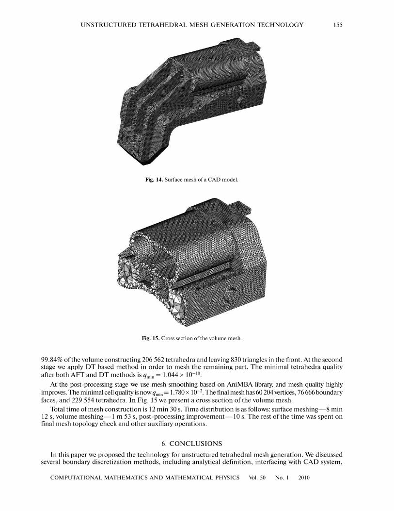
In this section we illustrate the use of an interface with OpenCASCADE CAD kernel. We tested ourCGM integration on a sample model 62_shaver1 from OpenCASCADE website [13]. The BREP modelhas 266 vertices, 403 edges, and 153 faces (see Fig. 13). The surface was meshed into a quasiuniform meshwith 38335 vertices and 76 666 triangles (see Fig. 14).

The combination of AFT and DT methods is used for volume meshing. At the first stage, we apply AFTmethod with automatic coarsening inside the domain with coarsening factor c = 1.0. AFT meshes only

(a) (b)

Fig. 12. Coarse dragon mesh: (a) coarsened survade mesh; (b) cross section of a volume.

Table 4.

Mesh qmin NT 10–1 10–2 10–3 10–4 10–5 10–6 10–7 10–8

AFT 1.965 × 10–7 102094 100733 1298 59 3 0 0 1 –

AFT + DT 1.129 × 10–9 105852 101942 2752 758 269 68 32 22 9

Smoothing 8.268 × 10–8 125383 115179 9945 244 13 0 0 0 2

Fig. 13. Original model in Open CASCADE CAD kernel.



99.84% of the volume constructing 206 562 tetrahedra and leaving 830 triangles in the front. At the secondstage we apply DT based method in order to mesh the remaining part. The minimal tetrahedra qualityafter both AFT and DT methods is qmin = 1.044 × 10–10.

At the post�processing stage we use mesh smoothing based on AniMBA library, and mesh quality highlyimproves. The minimal cell quality is now qmin = 1.780 × 10–2. The final mesh has 60 204 vertices, 76 666 boundaryfaces, and 229 554 tetrahedra. In Fig. 15 we present a cross section of the volume mesh.

Total time of mesh construction is 12 min 30 s. Time distribution is as follows: surface meshing—8 min12 s, volume meshing—1 m 53 s, post�processing improvement—10 s. The rest of the time was spent onfinal mesh topology check and other auxiliary operations.

6. CONCLUSIONS

In this paper we proposed the technology for unstructured tetrahedral mesh generation. We discussedseveral boundary discretization methods, including analytical definition, interfacing with CAD system,

Fig. 14. Surface mesh of a CAD model.

Fig. 15. Cross section of the volume mesh.

156


DANILOV

discrete surface modification, and CSG�based surface meshing. For robust volume meshing we proposedthe combination of two techniques: AFT as the primary method and DT as the fallback method. In com�bination with the post�processing tools, this technology produces tetrahedral meshes with good quality.Several application examples were demonstrated.

ACKNOWLEDGMENTS

This research was partly supported by the Russian Foundation for Basic Research through grant 08�01�00159�a and by RAS program “Optimal methods for problem of mathematical physics.”

The author thanks R. Garimella for the assistance with the abstracting interface layer with CAD sys�tems, and K. Nikitin for the CSG technology software. The author is grateful to Yu. Vassilevski for thelong�term support, fruitful discussions and valuable comments.

REFERENCES

1. E. Schönhardt, “Über die Zerlegung von Dreieckspolyedern in Tetraeder,” Math. Ann. 98, 309–312 (1928).2. B. Joe, “Three�Dimensional Boundary�Constrained Triangulations,” in Proc. 13th IMACS World Congress,

1992, pp. 215–222.3. P.�L. George and H. Borouchaki, “Maillage Simplicial d’un Polyédre Arbitraire,” C. R. Acad. Sci. Paris, Ser. I

338, 735–740 (2004).4. H. Borouchaki, F. Hecht, E. Saltel, and P.�L. George, “Reasonably Efficient Delaunay Based Mesh Generator

in 3 Dimensions,” in Proc. 4th Inernat. Meshing Roundtable, 1995, pp. 3–14.5. Q. Du and D. Wang, “Recent Progress in Robust and Quality Delaunay Mesh Generation,” J. Comput. Appl.

Math. 195, 8–23 (2006).6. J. R. Shewchuk, “Constrained Delaunay Tetrahedralizations and Provably Good Boundary Recovery,” in Proc.

11th Internat. Meshing Roundtable, 2002, pp. 193–204.7. Y. Ito, A. Shih, and B. Soni, “Reliable Isotropic Tetrahedral Mesh Generation Based on an Advancing Front

Method,” in Proc. 13th Internat. Meshing Roundtable, 2004, pp. 95–106.8. Y. Yang, J. Yong, and J. Sun, “An Algorithm for Tetrahedral Mesh Generation Based on Conforming Con�

strained Delaunay Tetrahedralization,” Comput. Graphics 29, 606–615 (2005).9. P.�L. George, H. Borouchaki, and E. Saltel, “Ultimate Robustness in Meshing an Arbitrary Polyhedron,” Inter�

nat. J. Numer. Meth. Engng. 58, 1061–1089 (2003).10. 3D Generator of Anisotropic Meshes, http://sourceforge.net/projects/ani3d/11. 2D Generator of Anisotropic Meshes, http://sourceforge.net/projects/ani2d/12. The Common Geometry Module, http://cubit.sandia.gov/cgm. html13. Open CASCADE Technology, http://www.opencascade.org/14. Yu. Vassilevski, A. Vershinin, A. Danilov, and A. Plenkin, Tetrahedral Mesh Generation in Domains Defined in

CAD Systems (Inst. Num. Math., Moscow, 2005), pp. 21–32 [in Russian].15. K. Nikitin, “Surface Meshing Technology for Domains Composed of Primitives,” Diploma Thesis (Dept. Mech.

Math., MSU, Moscow, 2007) [in Russian].16. P.�L. George and H. Borouchaki, “Delaunay Triangulation and Meshing,” in Application to Finite Elements

(Hermes, 1998).17. S. A. Ivanenko, “Variational Methods for Adaptive Grid Generation,” Comput. Math. Math. Phys. 42 (6),

830–844 (2003).18. V. Garanzha, “Max�Norm Optimization of Spatial Mappings with Application to Grid Generation, Construc�

tion of Surfaces and Shape Design,” in Proc. Minisymp. in Int. Conf. OFEA, 2001, pp. 61–74.19. A. Agouzal, K. Lipnikov, and Yu. Vassilevski, “Adaptive Generation of Quasi�Optimal Tetrahe�dral Meshes,”

East�West J. 7, 223–244 (1999).

unstructured tetrahedral mesh generation...

Documents