--

An Evaluation of Incentive Regulation

for Electric Utilities

by

Sanford V. BergUniversity of Florida

and

Jinook JeongUniversity of Florida

Abstract

This empirical study examines the determinants and impacts of incentive regulationsintroduced by utility commissions in the late '70s and early '80s. Rewards forgenerating plant utilization and low heat rates were found to have been introducedin states whose firms exhibited relatively high managerial slack (or relatively highercosts). However, the empirical results did not find that the introduction of specificcost component incentives improved overall operating cost Performance.

November 5, 1990(Revised)

The support of the Public Utility Research Center is gratefully acknowledged.Helpful suggestions were provided by Rashad Abdel-khalik, G.S. Maddala, DavidSappington and unidentified referees.

2

I. INTRODUCTION

In recent years, a number of state regulatory commissions have established "incentive regulation"

programs, to promote efficiency in electricity production. Unlike proposed price-cap regulations

which provide firms with a comprehensive incentive to control costs, these narrow incentive payment

programs condition financial rewards or penalties upon a specific measure of a utility's performance.

A program included in our data base is defined by the Edison Electric Institute (1987) as one which

"(i) is intended to improve regulated utilities' performance, (ii) evaluates utility performance against

specific, pre-defined standards, (iii) provides incentives (rewards) or disincentives (punishments),

depending on the utility's performance in relation to applicable standards," (p. 11).

These ~centivepayment programs take many forms and focus on different operating statistics:

they reward utilities which experience high levels of base load generating unit utilization and

availability, low heat rates (reflecting the efficient transformation of fuel into electricity), and keep

fuel and purchased power costs below externally-determined indices. For example, the State of

Florida adopted an incentive regulation entitled "Generating Performance Incentive Factor (GPIF)"

in 1980.1 The GPIF program sets the targets for many indicators including average heat rates, fuel

expenses, and past performance records etc. by complex formulas estimated by several computer

simulations of the utility system's economic dispatch. Rewards and penalties are imposed by

comparing actual performance with pre-set targets. Since we focus on an ex ante decoupling of prices

from cost components, expost prudence/efficiency reviews and management audits are excluded from

the programs examined here.

While the theoretical rationale for introducing incentive regulations is described elsewhere,2 the

1 For details, see Edison Electricity Institute (1987).

2 For example, see Joskow and Schmalensee (1986) or Johnson (1985).

3

effectiveness of incentive regulation has not been empirically tested. The purpose of this note is to

identify the determinants of regulatory initiatives in this area and to test the effectiveness of incentive

payment regulations in lowering electricity production costs. The questions asked in this paper

include:

1) What are the determinants of states adopting incentive regulations?

2) Did these incentive regulations accomplish their goal?

II. DATA

Annual data for 1973 - 1985 were collected from two sources: the Utility Compustat tape and

the Edison Electricity Institute's Incentive Regulation in the Electric Utility Industry - A Review of

Commissio,! Programs (1987). Although the overall sample included 53 utility companies for a 15

year period (795 potential observations), due to the missing data for some years, only 490

observations were actually available for estimation in a pooled data set. The firms in the data set are

listed in Table 1. Some descriptive statistics are reported in Table 2. Dropping the 14 firms with the

most missing observations entirely from the sample did not materially affect the results, so we report

the results for 53 firms.

ill. THE DETERMINANTS OF INCENTIVE REGULATION: UTILITY PERFORMANCE

The first issue to be addressed when evaluating incentive payment regulations for electric utilities

is the appropriate measure of utility performance. The actual measures which state commissions are

using vary, so a unique index is impossible to obtain.3 Two proxies for utility performance have

been utilized here: management slack and generation heat rate.

Selten (1986) and Abdel-khalik (1988) propose 'management slack' as an efficiency measure of

3 For details, see Edison Electricity Institute (1987).

utility's performance, defined as

Si == (CCCi*)/Ci

4

(1)

where Si is the managerial slack of firm i, Ci is log operating cost of firm i, and Ci* is the predicted

value of log operating cost for firm i. Si is the relative deviation of that firm's operating cost from

industry-wide average operating cost (at that output level). High Si would indicate that the firm's

performance is relatively inefficient, if all firms faced the same input prices and had available the

same technologies. Since a firm's generation mix at a given point of time depends on past and

projected demand growth and input price projections, operating costs can differ for reasons other

than managerial slack. However, we expect utility commissioners to compare costs of firms they

regulate wi~h those of comparable firms. Relatively high costs will trigger regulatory innovations

(Joskow, 1974).

Also, the heat rate, defined as the energy input in BTU used for 1 kwh electric generation, has

been widely used as a measure of operating efficiency.4 Higher heat rate has been interpreted as

inefficient performance. Of course, heat rates will differ across fJIttls due to many factors, including

average age of generating units (reflecting technological differences and historical demand growth

patterns), generating mix (base load vs. peaking capacity -- where the mix depends on seasonal and

daily demand patterns), and environmental regulations in place when capacity investments were made.

Thus, heat rates may not be a good proxy for relative efficiency.

Besides these proxies for utilities' performance, other variables can affect commissions' decisions

on the adoption of incentive regulations. First, we need to determine whether a commission's

adoption of incentive regulations depends on the firm's managerial slack or on heat rates, or both.

4 For example, Abdel-khalik (1988) and Landon (1985).

5

To test which one is the better proxy, the following Probit MLE model is estimated.

(2)

where, Ii = 1 when firm i is regulated by an incentive program

= 0 when firm i is not regulated by an incentive program

Si = the managerial slack of firm i (based on three years)

~ = the heat rate of firm i

MARi == (Total Revenue - Total Cost) / Total Cost

= firm i's margin

LOADF == total generation / (system capacity * 8760)

= the load factor of firm i

GENi = log of total generation of firm i.

A problem in the estimation of equation (2) is the endogeneity of Si. Si is endogenous in the

sense that the adoption of incentive regulations will affect utilities' managerial slack. To avoid the

endogeneity bias, observations are deleted in the following cases:5

1) For incentive-regulated firms, data are used only for the three years preceding incentive

regulation. For example, if incentive regulation starts in 1980, the firm's annual data for

1978, 1979 and 1980 are used. The firm is dropped from the sample in 1981 and beyond.

2) For non-incentive regulated firms, data after 1980 are deleted for estimating equation (2)

since incentive regulation lowered industry average oost--so that the non-regulated firms will

have higher measured managerial slack. 1980 is chosen because it is the mean of the starting

5 The remaining sample contains 156 observations.

6

year for payment incentive regulations. Note that non-incentive regulated firms are included

in the sample for the estimation of the operating cost equation.

The variables MAR, LOADF and GEN are included in equation (2) since other factors can also

trigger institutional innovations. We postulate that commissions will tend to adopt incentive

regulations if the electric utility has high prices relative to costs. In our model, higher margin does

not necessarily mean high cost of inefficiency because the margin is defined as "(revenue/cost) - 1"

and the average revenue varies more than the average cost in our data set. Thus, the margin is more

affected by the price (as approximated by average revenue) than the average cost (efficiency).6

Rate hearings can take a very long time to lower prices, while the introduction of an incentive which

targets gen<?rating unit availability or heat rates can. occur relatively quickly. The incentive regulation

can provide a mechanism for sharing further cost savings as well as for penalizing inefficiency.

Also, if a utility already has a high load factor, there is less opportunity for cost savings via rate

design changes which induce alterations in consumption patterns. Regulators would then press for

cost reductions via explicit incentive programs. In addition, we hypothesize that a large electric utility

(GEN) has greater political visibility. Furthermore, economic savings for large frrms will be greater

for equal percentage cost reductions. So we expect the signs on all three variables to be positive.

As noted earlier, the expected signs of a1 and a2 are also positive.

The slack index, Si (defined in equation 1) is obtained from the following operating cost function.

6 A reviewer noted that regulators might impose incentive payment regulation on firms with higher costsand low profits -- in order to provide an incentive for cost reduction and an opportunity for increasing therealized return on rate base. Thus, incentive regulation could be a disequilibrium phenomenon related to thechange in a firm's managerial slack relative to the industry average or to a change in the margin (holding allother factors constant). In such a situation, a continuing level of slack represents an improvement over whatmight have been a deteriorating trend. We interpret intervention as an equilibrium phenomenon, so relativelyhigher price-cost margins tends to trigger regulatory intervention. We did not investigate the impacts of changesin the explanatory variables.

7

where, Ci = log of the operating cost for firm i

RESCAPi = the reserve capacity of firm i

== (System Capacity - Peak Demand) / System Capacity

HYRi = log of the percentage of electricity produced by hydroelectric generation

NUC~ = log of the percentage of electricity produced by nuclear plants

YE~ = time variable (year), 1973-85

(3)

The es.timated parameters for the scale (GEN) variables will indicate the shape of the cost

function -- the extent of scale economies. High RESCAP can be interpreted as reflecting a

disequilibrium capacity situation--both level and mix. During this Period, most electric utilities had

forecasted substantial demand growth. When forecasts were not realized, firms were left with

excessive reserve margins. Hydro (HYR) and nuclear (NUCR) ought to be associated with lower

operating costs. The year was included to capture upward shifts in the cost function -- reflecting

wage inflation, rising fuel costs, and environmental expenses occurring during the second half of the

sample period.

The results of the cost function (3) are as follows:

C· = 17.221

(5.85)**- 5.59 GENi + 0.68 GENT - 0.02 GENI + 0.41 RESCAPi

(-5.35)** (5.58)** (-5.19)** (1.80)

+ 0.32 LOADFi + 0.009 HYRi - 0.02 NUC~ + 0.09~ + Vi(1.26) (0.938) (-4.80)** (19.86)** (4)

Adj. R2 = 0.81 F = 254.76 **

8

where the numbers in parenthesis are t-values and * (**) indicates the coefficient is significant at 5%

(1%) level. In (4), all the significant coefficients have expected signs and the model has good

explanatory power (adjusted R-squared is relatively high). Unless the model is seriously misspecified,

alternative specifications are not likely to affect our results?

Using Sj obtained from (4), the results obtained for equation (2) are the following:

~ = - 2.84(-1.14)

+ 277.10 Sj - 0.14 Hj + 1.14 MARj + 9.39 LOADFj(2.42)* (-1.11) (2.85)** (3.52)**

- 0.27 GENj + Uj(-1.72)

LR (LiJcelihood Ratio) = 20.034**Correct Prediction = 114/156 = 73.1 %

(5)

Equation (5) implies that state commissions adopt incentive regulation programs when the

utilities under their supervision exhibit high managerial slack. The other relevant variables have the

expected signs except GENj although it is not significant. The insignificant coefficient on GENj

indicates the size of electric utilities is not a key factor in the decision to introduce incentive

regulations.

In (5), the managerial slack is the better proxy for utilities' performance than heat rate. So, Sj

will be used as a proxy for electric utilities' performance in further estimation. Is the slack a proxy

for performance or a predictor of commissions' decision? In the analysis, commissions are assumed

to be efficient. In other words, they can precisely evaluate their utilities' performance. This

assumption is unavoidable in this kind of empirical study because the utilities' performances are not

7 To compare our results with other cost estimates, we re-estimated (4) without the cubic term. Explanatorypower drops, but the results are similar to those obtained by Atkinson and Halvorsen (1986). The re-calculationof Sj from this alternative specification does not change our conclusions.

·- .....~ '" .' ... ~ .- '" .- ..... ". '"." -.~" -----~....~:~~.

9

directly measurable. With this assumption, a good predictor of commissions' decision is, at the same

time, a good proxy for utilities' performance.

IV. EFFECTIVENESS OF INCENTIVE REGULATIONS

The second question in evaluating incentive regulations is whether or not they have been

successful. To test if the cost component incentive regulation programs have achieved their goals,

an ordinary dummy test can be conducted using the following equation.

(6)

where Di = 1 if the firm is under an incentive regulation

.Di .= 0 if the firm is not under an incentive regulation.

All the sample years are utilized in this test.

The parameter of interest is Y1 in equation (6). If Y1 is significantly negative, the adoption of

narrow incentive regulations has reduced the level of the utilities' slack. Thus, the hypothesis is

!Io:Yl=0 vs. H1:Yl<0.

However, the equation (6) cannot be estimated by OLS since Di is an endogenous variable. Di

is endogenous in the sense that the adoption of an incentive regulation depends on the level of the

managerial slack of the electric utilities. To obtain consistent estimators, the following simultaneous

equations model is considered.

(6)

(7)

where Ei and Wi are bivariate-normal and are independent of all the exogenous variables. This

10

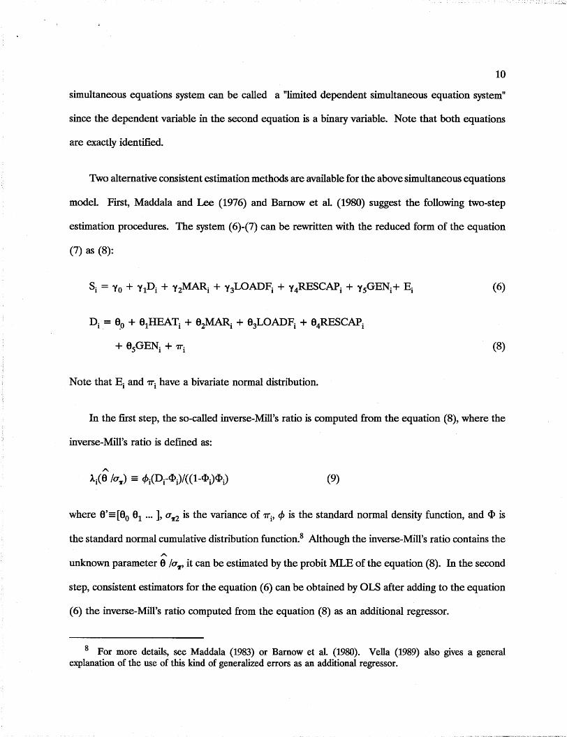
simultaneous equations system can be called a "limited dependent simultaneous equation system"

since the dependent variable in the second equation is a binary variable. Note that both equations

are exactly identified.

Two alternative consistent estimation methods are available for the above simultaneous equations

model. First, Maddala and Lee (1976) and Barnow et al. (1980) suggest the following two-step

estimation procedures. The system (6)-(7) can be rewritten with the reduced form of the equation

(7) as (8):

(6)

(8)

Note that E i and 7Ti have a bivariate normal distribution.

In the first step, the so-called inverse-Mill's ratio is computed from the equation (8), where the

inverse-Mill's ratio is defined as:

A.

li(8 luw) = c/>i(Dc<l>i)/«1-<I>i)<I>i) (9)

where 8'=[80 61 ••• ], uw2 is the variance of 7Ti, c/> is the standard normal density function, and <I> is

the standard normal cumulative distribution function.8 Although the inverse-Mill's ratio contains theA.

unknown parameter 8 luw' it can be estimated by the probit MLE of the equation (8). In the second

step, consistent estimators for the equation (6) can be obtained by OLS after adding to the equation

(6) the inverse-Mill's ratio computed from the equation (8) as an additional regressor.

8 For more details, see Maddala (1983) or Barnow et al. (1980). Vella (1989) also gives a generalexplanation of the use of this kind of generalized errors as an additional regressor.

11

An alternative consistent estimation proposed by Amemiya (1978), Heckman (1978), and Lee

(1979) is the following.9 First, estimate the equation (8) by probit MLE to obtain the predicted

values of Di, which are the predicted probabilities of the adoption of incentive regulation. Then, use

the predicted value as an instrumental variable for Di in the equation (6) to get consistent estimators

for 1/S. In this study, both estimation methods are used to test Ho : 11 = 0 vs. H1 : 11 < o.

v. ESTIMATION RESULTS

The profit MLE applied to the equation (8) gives the following results:

D. = ­1 6.4506

(-3.434)**- 0.1211 HEATi + 0.3877 MARi + 5.7033 LOADFi

(-1.315) (2.256)* (3.586)**

+ 1.5897 RESCAPi + 0.2827 GENi + 7Ti(1.840) (2.937)**

LR (Likelihood Ratio) = 36.728**Correct Prediction = 337/409 = 82.4 %

(10)

Note that this is the reduced form equation which is used as an intermediate result. Though the

structural parameters can be recovered from these reduced-form parameters, it is not necessary to

do since the equation of interest is the equation (6).

The two step estimation suggested by Maddala-Lee (1978) and Barnowet al. (1980) results in:

Si = - 0.0021 + OO2סס.0 Di - 0.0019 MARi - 0.0039 LOADFi(-1.777) (0.022) (-13.207)** (-3.441)**

+ OO2סס.0 RESCAPi + 0.0005 GENi + 0.0002 IMILLi + Ei(-0.033) (6.949)** (0.392)

Adj. R2 = 0.378110

(11)

9 The estimation method presented here is a simple version of Amemiya (1978), Heckman (1978), Lee(1979).

10 Note that the R2 in the two-step estimation does not have the same implications as in OLS because a'constructed'variable (inverse mill's ratio) is included in the second stage regression.

12

The hypothesis H o : Yl=0 vs. HI : Yl<0 is not rejected even at 10% significance level in (11).

This implies that the incentive regulations during 1973 - 1985 did not achieve the goal of reducing

the managerial slack of utility companies. We can also see in (11) that the slack is lower in more

profitable (higher margin) utilities, in high load factor utilities, and in smaller utilities. These results

seem reasonable. The results indicate that the reserve capacity of the utility does not affect the level

of managerial slack. This outcome may arise because slack is defined only in terms of operating costs.

The alternative N method produces a similar result. The estimated equation is:

Si = - 0.0013 + 0.0008 Di - 0.0020 MARi - 0.0047 LOADFi(-1.038) (0.843) (-13.305)** (-3.387)**

- 0.0002 RESCAPi + 0.0005 GENi. (-0.260) (6.148)**

Adj. R2 = 0.365011

(12)

The hypothesis Ho is not rejected with N method. Most of the parameters have the same sign

in both methods with an exception of RESCAP. The significance of explanatory variables are very

similar in both methods.

VI. SUMMARY AND CONCLUSIONS

The goal of specific target incentive payment regulations in electric production during 1968-1987

appears to be the reduction of managerial slack. However we did not find that the slack was

significantly reduced by narrow incentive regulations. A possible explanation is that by focusing on

specific categories or determinants of cost, regulators induce utilities to devote excessive resources

to ensuring that a narrow goal is reached--so no net cost savings are realized (Joskow and

11 This conventional R2 does not exactly measure the explained portion of the total variations since Di isan endogenous variable.

13

Schmalensee, 1986, p. 38; Berg and Tschirhart, 1988, p. 517-519).

One area for further research is investigating the duration of incentive programs. Some state

commissions discontinued their incentive regulation programs after several years. Our simultaneous

model only tested whether the existence of a program in that year had an impact -- yet some of these

programs were subsequently discontinued. By comparing these discontinued programs with the

continuing programs, one can better evaluate the impact of incentive regulations. It would also be

instructive to analyze the precise types of regulation in greater detail -- some types may have impacts

even if, on average, current incentive regulations fail to have measurable impacts. Similarly, patterns

within and across states could be examined. Although these are important questions, it is almost

impossible, .at this moment, to empirically analyze these issues because of data limitations.

Another direction for research is the introduction of political and administrative factors into the

model. For example Nowell and Tschirhart (1990) examined the determinants of state adoption of

PURPA, finding that political and interest group strength affect the probability of adopting the cost­

of service standard. Such factors could be introduced into the model. In another study of regulation,

Mathios and Rogers (1989) examined the impacts of different types of intra-state long distance

telephone regulation. They found that price-cap regimes lead to lower prices than rate-of return

regulation. However, their reduced form model does not take into account potential similaneity

problems regarding the determinants of states adopting different regulatory policies. The present

study of electricity regulation attempts to avoid that problem.

Joskow (1974) noted how regulatory innovations were introduced during economic dislocations

(the advent of inflation and new environmental laws). Similarly, we can identify early incentive

regulations as stemming from concerns with managerial slack. Our inability to find an impact of cost

component regulation suggests that either the factors affecting performance are not adequately

14

captured in our model specification, or that this particular type of regulatory innovation has failed

to achieve its goal of increased efficiency. If incentive regulation is to be adopted, more

comprehensive schemes (such as price caps) might warrant greater attention.

CUSIP

255374055541033

125896144141152357154051155033155771202795207597210615257470264399277173370550449495452092462416462470462524542671591894595832598319629140644001644188653522664397665772694308695114708696709051717537

Table 1Organizations in the data set

COMPANY

American Electric PowerArizona Public Service Co.Arkansas Power and LightCMS Energy Corp.Carolina Power and LightCentral and South West Corp.Central Maine Power Co.Central Power and LightCentral Vermont Pub. ServiceCommonwealth EdisonConnecticut Light and PowerConsumers Power Co..Dominion Resources Inc-VADuke Power Co.Eastern Utilities Assoc.General Public UtilitiesI.E. Industries Inc.Illinois Power Co.Iowa Electric Light and PowerIowa-lllinois Gas and Elec.Iowa Public Service Co.Long Island LightingMetropolitan EdisonMiddle South UtilitiesMidwest Energy Co.Nipsco Industries Inc.New England Electric SystemNew England PowerNiagara Mohawk PowerNortheast UtilitiesNorthern States Power-MNPacific Gas and ElectricPacificorpPennsylvania Electric Co.Pennsylvania Power and LightPhiladelphia Electric Co.

15

PERIOD OFINCENTIVE REG.

74 - present*84 - present81 - presentN/A**78 - 81N/AN/AN/AN/AN/A79 - present78 - 83N/A78 - 8181 - presentN/AN/AN/AN/AN/AN/AN/A80 - presentN/AN/AN/A81 - present81 - present82 - present81 - presentN/A83 - presentN/A80 - present80 - present85 - present

* 'present' means 1987.** N/A: no incentive regulation

CUSIP

723484736506736508744482771367805898837004842400842587880591906548927804929305958587976656976657976843

Table 1 (continued)

COMPANY

Pinnacle West Capital Corp.Portland General Corp.Portland General Electric Co.Public Service Co. of N. H.Rochester Gas and ElectricScana Corp.South Carolina Elec. & Gas Co.Southern Calif. Edison Co.Southern Co.Tennessee Valley AuthorityUnion Electric Co.Virginia Elec. and Power Co.WPL Holdings Inc.Western Massachusetts El. Co.Wisconsin Electric Power Co.Wisconsin Energy Corp.Wisconsin Public Service

16

PERIOD OFINCENTIVE REG.

N/AN/A80 - present82 - present83 - presentN/AN/A81 - presentN/AN/AN/AN/AN/A81 - presentN/AN/AN/A

* 'present'means 1987.** N/A: no incentive regulation

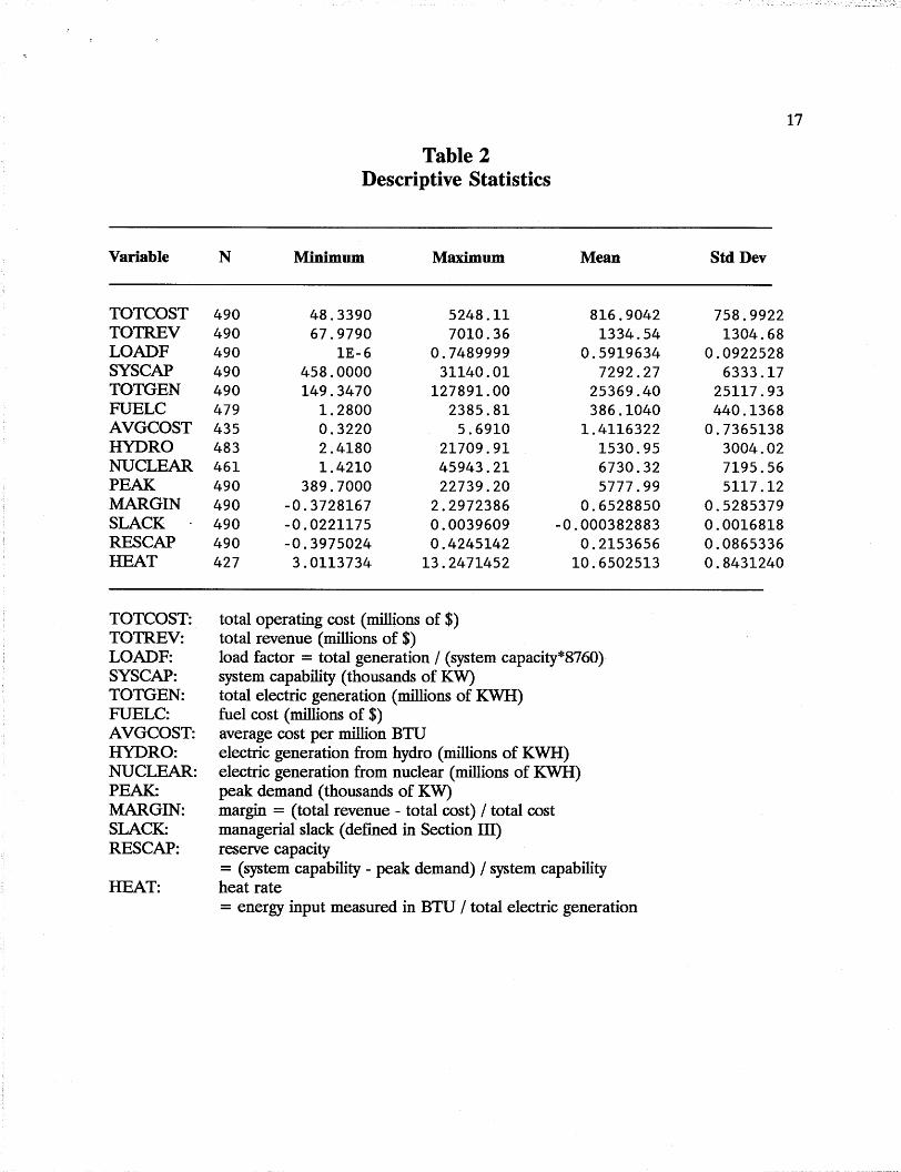
Table 2Descriptive Statistics

17

Variable N Minimum Maximum Mean Std Dev

TOTCOST 490 48.3390 5248.11 816.9042 758.9922TOTREV 490 67.9790 7010.36 1334.54 1304.68LOADF 490 lE-6 0.7489999 0.5919634 0.0922528SYSCAP 490 458.0000 31140.01 7292.27 6333.17TOTGEN 490 149.3470 127891.00 25369.40 25117.93FUELC 479 1.2800 2385.81 386.1040 440.1368AVGCOST 435 0.3220 5.6910 1.4116322 0.7365138HYDRO 483 2.4180 21709.91 1530.95 3004.02NUCLEAR 461 1.4210 45943.21 6730.32 7195.56PEAK 490 389.7000 22739.20 5777.99 5117.12MARGIN 490 -0.3728167 2.2972386 0.6528850 0.5285379SLACK 490 -0.0221175 0.0039609 -0.000382883 0.0016818RESCAP 490 -0.3975024 0.4245142 0.2153656 0.0865336HEAT 427 3.0113734 13.2471452 10.6502513 0.8431240

TOTCOST: total operating cost (millions of $)TOTREV: total revenue (millions of $)LOADF: load factor = total generation / (system capacity*8760)SYSCAP: system capability (thousands of KW)TOTGEN: total electric generation (millions of KWH)FUELC: fuel cost (millions of $)AVGCOST: average cost per million BTUHYDRO: electric generation from hydro (millions of KWH)NUCLEAR: electric generation from nuclear (millions of KWH)PEAK: peak demand (thousands of KW)MARGIN: margin = (total revenue - total cost) / total costSLACK: managerial slack (defined in Section ill)RESCAP: reserve capacity

= (system capability - peak demand) / system capabilityHEAT: heat rate

= energy input measured in BTU / total electric generation

18

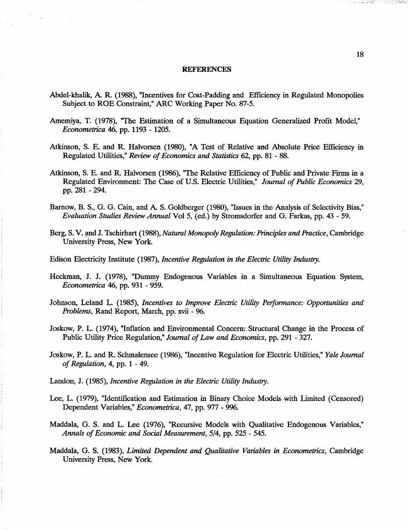
REFERENCES

Abdel-khalik, A R. (1988), "Incentives for Cost-Padding and Efficiency in Regulated MonopoliesSubject to ROE Constraint," ARC Working Paper No. 87-5.

Amemiya, T. (1978), "The Estimation of a Simultaneous Equation Generalized Profit Model,"Econometrica 46, pp. 1193 - 1205.

Atkinson, S. E. and R. Halvorsen (1980), "A Test of Relative and Absolute Price Efficiency inRegulated Utilities," Review ofEconomics and Statistics 62, pp. 81 - 88.

Atkinson, S. E. and R. Halvorsen (1986), "The Relative Efficiency of Public and Private Firms in aRegulated Environment: The Case of U.S. Electric Utilities," Journal of Public Economics 29,pp. 281 - 294.

Barnow, B. S., G. G. Cain, and A S. Goldberger (1980), "Issues in the Analysis of Selectivity Bias,"Evaluation Studies Review Annual Vol 5, (ed.) by Stromsdorfer and G. Farkas, pp. 43 - 59.

Berg, S. V. ~nd J. Tschirhart (1988), Natural Monopoly Regulation: Principles and Practice, CambridgeUniversity Press, New York.

Edison Electricity Institute (1987), Incentive Regulation in the Electric Utility Industry.

Heckman, J. J. (1978), "Dummy Endogenous Variables in a Simultaneous Equation System,Econometrica 46, pp. 931 - 959.

Johnson, Leland L. (1985), Incentives to Improve Electric Utility Performance: Opportunities andProblems, Rand Report, March, pp. xvii - 96.

Joskow, P. L. (1974), "Inflation and Environmental Concern: Structural Change in the Process ofPublic Utility Price Regulation," Journal ofLaw and Economics, pp. 291 - 327.

Joskow, P. L. and R. Schmalensee (1986), "Incentive Regulation for Electric Utilities," Yale Journalof Regulation, 4, pp. 1 - 49.

Landon, J. (1985), Incentive Regulation in the Electric Utility Industry.

Lee, L. (1979), "Identification and Estimation in Binary Choice Models with Limited (Censored)Dependent Variables," Econometrica, 47, pp. 977 - 996.

Maddala, G. S. and L. Lee (1976), "Recursive Models with Qualitative Endogenous Variables,"Annals ofEconomic and Social Measurement, 5/4, pp. 525 - 545.

Maddala, G. S. (1983), Limited Dependent and Qualitative Variables in Econometrics, CambridgeUniversity Press, New York.

19

Mathios, A D. and R. P. Rogers (1989), "The Impact of Alternative Forms of State Regulationof AT&T on Direct-Dial, Long Distance Telephone Rates," Rand Journal ofEconomics, Vol.20, No.3, pp. 437 - 453.

Nowell, C. and J. Tschirhart (1990), "The Public Utility Regulatory Policy Act and RegulatoryBehavior," Journal of Regulatory Economics, Vol. 2, No.1, pp. 21 - 36.

Selten, R. (1986), "Elementary Theory of Slack-ridden Imperfect Competition," New Developmentsin the Analysis ofMarket Structure, ed. by Stiglitz J.E. and G.F. Mathewson, MIT Press.

Vella, F. (1989), "A Simple Estimator for Simultaneous Models with Censored EndogenousRegressors," Unpublished Manuscript, University of Rochester.