university of pennsylvania 10/5/00cse 3801 cpu scheduling cse 380 lecture note 9 insup lee
Post on 19-Dec-2015
214 views
TRANSCRIPT

10/5/00 CSE 380 1
University of Pennsylvania
CPU Scheduling
CSE 380
Lecture Note 9
Insup Lee

10/5/00 CSE 380 2
University of Pennsylvania
CPU SCHEDULING
• The basic problem is as follows: How can OS schedule the allocation of CPU cycles to processes in system, to achieve “good performance”?
• Components of CPU scheduling subsystem of OS:
– Dispatcher - performs context switches
– Scheduler - selects next process from those in main memory (short-term scheduler)
– Swapper - manages transfer of processes between main memory and secondary storage (medium-term scheduler)
– Long-Term Scheduler - in a batch system, determines which and how many jobs to admit into system.

10/5/00 CSE 380 3
University of Pennsylvania
Behavior of Processes in Execution
• Useful concept in context of scheduling:
– CPU Burst - period of CPU time process is executing between I/O requests. The text also talks about “I/O burst”.
• Processes alternate between CPU & I/O bursts:
– CPU I/O CPU I/O CPU ... I/O CPU
• CPU-bound process uses CPU for long periods of time.
• I/O-bound process uses CPU briefly before it issues another I/O request.
• In interactive system, usually important to have fast response time. Accomplished by having scheduler favor I/O-bound processes.
• Necessary to determine as quickly as possible the nature (CPU-bound or I/O-bound) of a process, since usually not known in advance.

10/5/00 CSE 380 4
University of Pennsylvania
General Organization for CPU Scheduling
• Processes ready to use CPU are kept in a ready queue.
• Processes waiting for I/O are kept in wait queue associated with device on which they are performing I/O.
• Dispatcher: called from timer interrupt or when current process blocks for I/O performs a context switch to first process in ready queue
• Scheduler: called periodically, usually less often than dispatcher. Reorders ready queue to reflect changing priorities.
• Swapper: keeps track of “process mix'' in main memory. If CPU utilization not high enough, processes can be “swapped” between main memory and a swap area on secondary storage.
10/5/00 CSE 380 5
University of Pennsylvania
Types of Scheduling Algorithms
• Preemptive: process may have CPU taken away before completion of current CPU burst
• Non-preemptive: processes always run until CPU burst completes
• Static Priority
• Dynamic Priority

10/5/00 CSE 380 6
University of Pennsylvania
Performance Criteria for Scheduling
• Scheduling (as an Optimization task): How to best order the ready queue for efficiency purposes.
• CPU utilization: % of time CPU in use
• Throughput: # of jobs completed per time unit
• Turnaround Time: wall clock time required to complete a job
• Waiting Time: amount of time process is ready but waiting to run
• Response Time: in interactive systems, time until system responds to a command
• Response Ratio: (Turnaround Time)/(Execution Time) -- long jobs should wait longer
• The overhead of a scheduling algorithm (e.g., data kept about execution activity, queue management, context switches) should also be taken into account.

10/5/00 CSE 380 7
University of Pennsylvania
Kleinrock's Conservation Law
No matter what scheduling algorithm is used, you cannot help one class of jobs without hurting the other ones.
Example: A minor improvement for short jobs (say, on waiting time) causes a disproportionate degradation for long jobs.

10/5/00 CSE 380 8
University of Pennsylvania
Basic Scheduling Algorithm
• FCFS - First-Come, First-Served
– Non-preemptive
– Ready queue is a FIFO queue
– Jobs arriving are placed at the end of queue
– Dispatcher selects first job in queue and runs to completion of CPU burst
• Advantages: simple, low overhead
• Disadvantages: inappropriate for interactive systems, large fluctuations in average turnaround time are possible.

10/5/00 CSE 380 9
University of Pennsylvania
FCFS Example
Pid Arr CPU Start Finish Turna Wait Ratio---+---+---+-----+------+-----+----+----- A 0 3 0 3 3 0 1.0 B 1 5 3 8 7 2 1.4 C 3 2 8 10 7 5 3.5 D 9 5 10 15 6 1 1.2 E 12 5 15 20 8 3 1.6
---+---+---+-----+------+-----+----+----- A 0 1 0 1 1 0 1.00 B 0 100 1 101 101 1 1.01 C 0 1 101 102 102 101 102.00 D 0 100 102 202 202 102 2.02

10/5/00 CSE 380 10
University of Pennsylvania
RR - Round Robin
• Preemptive version FCFS
• Treat ready queue as circular
– arriving jobs are placed at end
– dispatcher selects first job in queue and runs until completion of CPU burst, or until time quantum expires
– if quantum expires, job is again placed at end

10/5/00 CSE 380 11
University of Pennsylvania
Properties of RR
Advantages: simple, low overhead, works for interactive systems
Disadvantages: if quantum too small, too much time wasted in context switching; if too large, approaches FCFS.Typical value: 10 - 100 msecRule of thumb: choose quantum so that large majority (80-90%) of jobs finish CPU burst in one quantum

10/5/00 CSE 380 12
University of Pennsylvania
SJF - Shortest Job First
• non-preemptive
• ready queue treated as a priority queue based on smallest CPU-time requirement
– arriving jobs inserted at proper position in queue
– dispatcher selects shortest job (1st in queue) and runs to completion
Advantages: provably optimal w.r.t. average turnaround time
Disadvantages: in general, unimplementable. Also, starvation possible!
Can do it approximately: use exponential averaging to predict length of next CPU burst ==> pick shortest predicted burst next!
10/5/00 CSE 380 13
University of Pennsylvania
Exponential Averaging
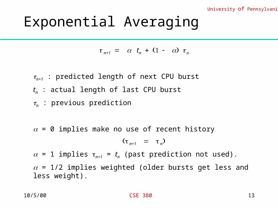
n+1 tn n
n+1 : predicted length of next CPU burst
tn : actual length of last CPU burst
n : previous prediction
= 0 implies make no use of recent history
n+1 n
= 1 implies n+1 = tn (past prediction not used).
= 1/2 implies weighted (older bursts get less and less weight).

10/5/00 CSE 380 14
University of Pennsylvania
SRTF - Shortest Remaining Time First
• Preemptive version of SJF
• Ready queue ordered on length of time till completion (shortest first)
• Arriving jobs inserted at proper position
• Dispatcher selects shortest job and runs to completion or until a job with a shorter remaining time arrives in the system.

10/5/00 CSE 380 15
University of Pennsylvania
Performance Evaluation
• Deterministic Modeling (vs. Probabilistic) Look at behavior of algorithm on a particular workload, and compute various performance criteria
Example:
workload - Job 1: 24 units Job 2: 3 units Job 3: 3 units
• Gantt chart for FCFS:
| Job 1 | Job 2 | Job 3 | 0 24 27 30
Total waiting time: 0 + 24 + 27 = 51
Average waiting time: 51/3 = 17
Total turnaround time: 24 + 27 + 30 = 81
Average turnaround time: 81/3 = 9

10/5/00 CSE 380 16
University of Pennsylvania
RR and SJF
• Chart for RR with quantum of 3:
| Job 1 | Job 2 | Job 3 | Job 1 | 0 3 6 9 30
Total waiting time: 6 + 6 + 3 = 15
Avg. waiting time: 15 / 3 = 5
• Chart for SJF:
| Job 2 | Job 3 | Job 1 | 0 3 6 30
Total waiting time: 6 + 0 + 3 = 9
Avg. waiting time: 9 / 3 = 3
• Can see that SJF gives minimum waiting time. RR is intermediate. (This can be proved in general.)

10/5/00 CSE 380 17
University of Pennsylvania
HPF - Highest Priority First
• general class of algorithms
• each job assigned a priority which may change dynamically
• may be preemptive or non-preemptive
Problem: how to compute priorities?
10/5/00 CSE 380 18
University of Pennsylvania
Multi-Level Feedback (FB)
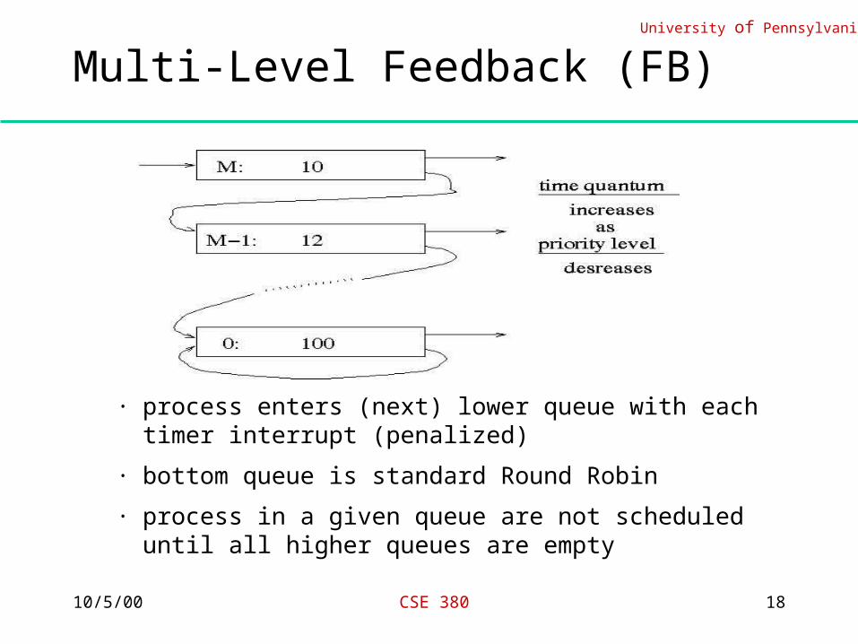
· process enters (next) lower queue with each timer interrupt (penalized)
· bottom queue is standard Round Robin
· process in a given queue are not scheduled until all higher queues are empty

10/5/00 CSE 380 19
University of Pennsylvania
FB Discussion
I/O-bound processes tend to congregate in higher-level queues. (Why?)
Nice, since obtain greater device utilization
Quantum in top queue should be large enough to satisfy majority of I/O-bound processes
Variations – Priority can assign a process a lower priority by starting it at a lower-level
queue
can raise priority by moving process to a higher queue can use in conjunction with aging
Adaptive to adjust priority of a process changing from CPU-bound to I/O-
bound, can move process to a higher queue each time it voluntarily relinquishes CPU.
10/5/00 CSE 380 20
University of PennsylvaniaShort-term Process Scheduling in 4.3 BSD• based on multi-level feedback queues
• priorities range from 0 to 127
• 0-49 reserved for processes executing in kernel mode
• 50-127 reserved for scheduling processes in user mode
• number of queues 127 in theory; 32 in VAX
• time quantum = 1/10 sec (empirically found to be the longest quantum that could be used without loss of the desired response for interactive jobs such as editors)
– short time quantum means better interactive response
– long time quantum means higher overall system throughput since less context switch overhead and less processor cache flush.
• priority dynamically adjusted to reflect
– resource requirement (e.g., blocked awaiting an event)
– resource consumption (e.g., CPU time)
10/5/00 CSE 380 21
University of Pennsylvania
Unix CPU scheduler (cont.)
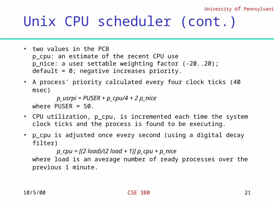
• two values in the PCBp_cpu: an estimate of the recent CPU usep_nice: a user settable weighting factor (-20..20); default = 0; negative increases priority.
• A process' priority calculated every four clock ticks (40 msec)p_usrpi = PUSER + p_cpu/4 + 2 p_nice
where PUSER = 50.
• CPU utilization, p_cpu, is incremented each time the system clock ticks and the process is found to be executing.
• p_cpu is adjusted once every second (using a digital decay filter)p_cpu = [(2 load)/(2 load + 1)] p_cpu + p_nice
where load is an average number of ready processes over the previous 1 minute.

10/5/00 CSE 380 22
University of Pennsylvania
Examples
Example 1. single compute-bound process which monopolizes CPU.
p_cpu = 0.66 p_cpu + p_nice
Example 2. this process accumulates Ti clock ticks every 1 second and p_nice is zero.
p_cpu = 0.66 T0
p_cpu = 0.66 (T1 + .66 T0) = .66 T1 + .44 T0
p_cpu = 0.66 T2 + .44 T1 + .30 T0
p_cpu = 0.66 T3 + ... + .20 T0
p_cpu = 0.66 T4 + ... + .13 T0
About 90 % of the CPU utilization is forgotten after 5 seconds.

10/5/00 CSE 380 23
University of Pennsylvania
For blocked process,
the system recomputes the priority of a process when the process is awakened and has been sleeping for longer than 1 second.
p_slptime is set to 0 when a process starts sleep and is incremented once every second.
when the process is awakened,
p_cpu = [2 load/(2 load +1)]p_slptime p_cpu
Then, computes p_usrpri as above.

10/5/00 CSE 380 24
University of Pennsylvania
Real-time Systems
• On-line transaction systems and interaction systems
• Real-time monitoring systems
• Signal processing systems
o typical computations
o timing requirements
o typical architectures
• Control systems
o computational and timing requirements of direct computer control
o hierarchical structure
o intelligent control

10/5/00 CSE 380 25
University of Pennsylvania
Desired characteristics of RTOS
Predictability, not speed, fairness, etc.
• Under normal load, all deterministic (hard deadline) tasks meet their timing constraints
• under overload conditions, failures in meeting timing constrains occur in a predictable manner.
Interrupt handling and context switching take bounded times
Application- directed resource management
• scheduling mechanisms allow different policies
• resolution of resource contention can be under explicit direction of the application.
10/5/00 CSE 380 26
University of Pennsylvania
Real-Time System Scheduling
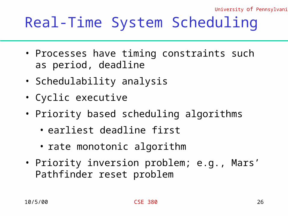
• Processes have timing constraints such as period, deadline
• Schedulability analysis
• Cyclic executive
• Priority based scheduling algorithms
• earliest deadline first
• rate monotonic algorithm
• Priority inversion problem; e.g., Mars’ Pathfinder reset problem

10/5/00 CSE 380 27
University of Pennsylvania
The Priority Inversion Problem
T1
T2
T3
blocked attempt lock R lock(R)
lock(R)
unlock(R)
unlock(R)
10/5/00 CSE 380 28
University of Pennsylvania
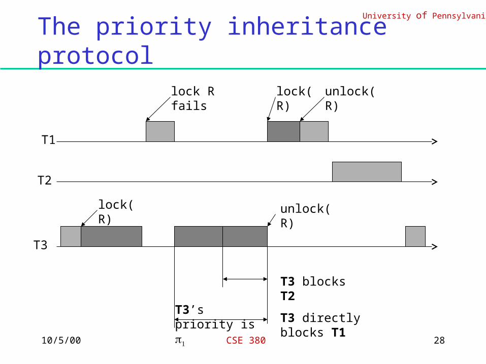
The priority inheritance protocol
T1
T2
T3
lock R fails lock(R)
lock(R)
unlock(R)
unlock(R)
T3 blocks T2
T3 directly blocks T1T3’s priority is