University of Groningen

A graph-theoretical approach for the analysis and model reduction of complex-balancedchemical reaction networksRao, Shodhan; Schaft, Arjan van der; Jayawardhana, Bayu

Published in:Journal of Mathematical Chemistry

DOI:10.1007/s10910-013-0218-8

IMPORTANT NOTE: You are advised to consult the publisher's version (publisher's PDF) if you wish to cite fromit. Please check the document version below.

Document VersionPublisher's PDF, also known as Version of record

Publication date:2013

Link to publication in University of Groningen/UMCG research database

Citation for published version (APA):Rao, S., Schaft, A. V. D., & Jayawardhana, B. (2013). A graph-theoretical approach for the analysis andmodel reduction of complex-balanced chemical reaction networks. Journal of Mathematical Chemistry,51(9), 2401-2422. https://doi.org/10.1007/s10910-013-0218-8

CopyrightOther than for strictly personal use, it is not permitted to download or to forward/distribute the text or part of it without the consent of theauthor(s) and/or copyright holder(s), unless the work is under an open content license (like Creative Commons).

Take-down policyIf you believe that this document breaches copyright please contact us providing details, and we will remove access to the work immediatelyand investigate your claim.

Downloaded from the University of Groningen/UMCG research database (Pure): http://www.rug.nl/research/portal. For technical reasons thenumber of authors shown on this cover page is limited to 10 maximum.

Download date: 21-04-2020

J Math Chem (2013) 51:2401–2422DOI 10.1007/s10910-013-0218-8

ORIGINAL PAPER

A graph-theoretical approach for the analysisand model reduction of complex-balancedchemical reaction networks

Shodhan Rao · Arjan van der Schaft ·Bayu Jayawardhana

Received: 25 March 2013 / Accepted: 18 June 2013 / Published online: 3 July 2013© Springer Science+Business Media New York 2013

Abstract In this paper we derive a compact mathematical formulation describingthe dynamics of chemical reaction networks that are complex-balanced and are gov-erned by mass action kinetics. The formulation is based on the graph of (substrateand product) complexes and the stoichiometric information of these complexes, andcrucially uses a balanced weighted Laplacian matrix. It is shown that this formulationleads to elegant methods for characterizing the space of all equilibria for complex-balanced networks and for deriving stability properties of such networks. We proposea method for model reduction of complex-balanced networks, which is similar to theKron reduction method for electrical networks and involves the computation of Schurcomplements of the balanced weighted Laplacian matrix.

Keywords Weighted Laplacian matrix · Linkage classes · Zero-deficiencynetworks · Persistence conjecture · Equilibria · Schur complement

Mathematics Subject Classification 05C50 · 34D05 · 34D20 · 93A15 · 93C15

S. Rao (B)Center for Systems Biology, University of Groningen, Groningen, The Netherlandse-mail: shodhanr@gmail.com; s.rao@umcg.nl

A. van der SchaftJohann Bernoulli Institute for Mathematics and Computer Science, University of Groningen,Groningen, The Netherlandse-mail: A.J.van.der.Schaft@rug.nl

B. JayawardhanaInstitute of Technology and Management, University of Groningen, Groningen,The Netherlandse-mail: b.jayawardhana@rug.nl

123

2402 J Math Chem (2013) 51:2401–2422

1 Introduction

One of the issues in formalizing the dynamics of chemical reaction networks is thefact that their graph representation is not immediate; due to the fact that chemicalreactions usually involve more than one substrate chemical species and more than oneproduct chemical species. This problem is resolved by associating the complexes of thereactions, i.e. the left-hand (substrate) and right-hand (product) sides of each reaction,with the vertices of a graph, and the reactions with the edges.1 The resulting directedgraph, called the graph of complexes, is characterized by its incidence matrix B.Furthermore the stoichiometric matrix S of the chemical reaction network, expressingthe basic balance laws of the reactions, can be factorized as S = Z B, with the complex-stoichiometric matrix Z encoding the expressions of the complexes in the variouschemical species. We note that an alternative graph formulation of chemical reactionnetworks is the species-reaction graph [2–4,7], which is a bipartite graph with one partof the vertices corresponding to the species and the remaining part to the reactions,and the edges expressing the involvement of the species in the reactions.

Using the graph of complexes formalism, we have developed in [23,28] a compactmathematical formulation for a class of mass-action kinetics chemical reaction net-works, which is characterized by the assumption of the existence of an equilibriumfor the reaction rates; a so-called thermodynamic equilibrium. This corresponds to thethermodynamically justified assumption of microscopic reversibility, with the result-ing conditions on the parameters of the mass action kinetics usually referred to as theWegscheider conditions. The resulting class of mass action kinetics reaction networksare called (detailed)-balanced. A main feature of the formulation of [28] is the fact thatthe dynamics of a detailed-balanced chemical reaction network is completely specifiedby a symmetric weighted Laplacian matrix, defined by the graph of complexes and theequilibrium constants, together with an energy function, which is subsequently usedfor the stability analysis of the network. In particular, the resulting dynamics is shown[23] to bear close similarity with consensus algorithms for symmetric multi-agentsystems. (In fact, it is shown in [28] that the so-called complex-affinities asymptoti-cally reach consensus.) Furthermore, as shown in [17], the framework can be readilyextended from mass action kinetics to (reversible) Michaelis-Menten reaction rates.

On the other hand, the assumption of existence of a thermodynamical equilibriumrequires reversibility of all the reactions of the network, while there are quite a fewwell-known irreversible chemical reaction network models, including the McKeithannetwork to be explained shortly afterwards. Motivated by such examples we will extendin this paper the results of [28] by considering the substantially larger class of complex-balanced reaction networks. A chemical reaction network is called complex-balancedif there exists a vector of species concentrations at which the combined rate of outgoingreactions from any complex is equal to the combined rate of incoming reactions tothe complex, or in other words each of the complexes involved in the network is atequilibrium. The notion of complex-balanced networks was first introduced in [16]

1 This approach is originating in the work of Horn and Jackson [16]; see also Othmer [21] and [2] for niceexposés and additional insights.

123

J Math Chem (2013) 51:2401–2422 2403

Fig. 1 McKeithan’s network

and studied in detail in [8,9,11,15,24]. These systems have also been called toricdynamical systems in the literature (see [8]).

An example of a complex-balanced network is the model of T-cell interactions dueto [19] (see also [25]) depicted in Fig. 1. This chemical reaction network model arisesin immunology and was proposed by McKeithan in order to explain the selectivityof T-cell interactions. With reference to Fig. 1, T and M represent a T-cell receptorand a peptide-major histocompatibility complex (MHC) respectively and T + M isa complex for the network. For i = 1, . . . , N , Ci represent various intermediatecomplexes in the phosphorylation and other intermediate modifications of the T-cellreceptor T ; kp,i represents the rate constant of the i th step of the phosphorylationand k−1,i is the dissociation rate of the i th complex. In the following, we denote by[A] the concentration of a species A participating in a chemical reaction network.The governing law of the reaction network is the law of mass action kinetics. Thisleads to the following set of differential equations describing the rate of change ofconcentrations of various species involved in the network:

d[T ]dt

= d[M]dt

= −kp,0[T ][M] +N∑

i=0

k−1,i [Ci ]

d[C0]dt

= kp,0[T ][M] − (k−1,0 + kp,1

) [C0]...

d[Ci ]dt

= kp,i [Ci−1] − (k−1,i + kp,i+1

) [Ci ]...

d[CN ]dt

= kp,N [CN−1] − k−1,N [CN ] (1)

Observe that if the left hand side of each of the above equations is set to zero, allthe concentrations [Ci ] for i = 0, . . . , N − 1, can be parametrized in terms of [CN ].Since all the rate constants and dissociation constants are positive, it is easy to seethat there exists a set of positive concentrations {[T ], [M], [C0], . . . , [CN ]} for whichthe right hand sides of the Eq. (1) vanish. This implies that McKeithan’s network iscomplex-balanced. On the other hand, all reactions in this network are irreversible,and thus McKeithan’s network is not detailed-balanced.

The main aim of this paper is to show how the compact mathematical formula-tion of detailed-balanced chemical reaction networks derived in [28] can be extendedto complex-balanced networks (such as McKeithan’s network). Indeed, the crucial

123

2404 J Math Chem (2013) 51:2401–2422

difference between detailed-balanced and complex-balanced networks will turn outto be that in the latter case the Laplacian matrix is not symmetric anymore, but stillbalanced (in the sense of the terminology used in graph theory and multi-agent dynam-ics). In particular, complex-balanced chemical networks will be shown to bear closeresemblance with asymmetric consensus dynamics with balanced Laplacian matrix.Exploiting this formulation it will be shown how the dynamics of complex-balancednetworks share important common characteristics with those of detailed-balanced net-works, including a similar characterization of the set of all equilibria and the samestability result stating that the system converges to an equilibrium point uniquely deter-mined by the initial condition. For the particular case when the complex-stoichiometricmatrix Z is injective as in the McKeithan’s network case, the same asymptotic sta-bility results were obtained before in [25]. Furthermore, while for detailed-balancednetworks it has been shown in [28] that all equilibria are in fact thermodynamic equi-libria in this paper the similar result will be proved that all equilibria of a complex-balanced network are complex-equilibria. Similar results have already been proved in[16]; however, the proofs presented in the current paper are much more concise andinsightful as compared to those presented in [16].

Furthermore, based on our formulation of complex-balanced networks exhibiting abalanced weighted Laplacian matrix associated to the graph of complexes, we will pro-pose a technique for model-reduction of complex-balanced networks. This techniqueis similar to the Kron reduction method for model reduction of resistive electrical net-works described in [18]; see also [10,27]. Our technique works by deleting complexesfrom the graph of complexes associated with the network. In other words, our reducednetwork has fewer complexes and usually fewer reactions as compared to the originalnetwork, and yet the behavior of a number of significant metabolites in the reducednetwork is approximately the same as in the original network. Thus our model reduc-tion method is useful from a computational point of view, specially when we need todeal with models of large-scale complex-balanced chemical reaction networks. Math-ematically our approach is based on the result that the Schur complement (with respectto the deleted complexes) of the balanced weighted Laplacian matrix of the full graphof complexes is again a balanced weighted Laplacian matrix corresponding to thereduced graph of complexes.

The paper is organized as follows. In Sect. 2, we introduce tools from graph theoryand stoichiometry of reactions that are required to derive our mathematical formu-lation. In Sect. 3, we explain mass action kinetics, define complex-equilibria andcomplex-balanced networks and then derive our formulation. In Sect. 4, we deriveequilibrium and stability properties of complex-balanced networks using our formula-tion. In Sect. 5, we propose a model reduction method for complex-balanced networks,while Sect. 6 presents conclusions based on our results.

Notation The space of n dimensional real vectors is denoted by Rn , and the space of

m ×n real matrices by Rm×n . The space of n dimensional real vectors consisting of all

strictly positive entries is denoted by Rn+ and the space of n dimensional real vectors

consisting of all nonnegative entries is denoted by Rn+. The rank of a real matrix A is

denoted by rank A. dim(V) denotes the dimension of a set V . Given a1, . . . , an ∈ R,

123

J Math Chem (2013) 51:2401–2422 2405

diag(a1, . . . , an) denotes the diagonal matrix with diagonal entries a1, . . . , an ; thisnotation is extended to the block-diagonal case when a1, . . . , an are real square matri-ces. Furthermore, ker A and span A denote the kernel and span respectively of a realmatrix A. If U denotes a linear subspace of R

m , then U⊥ denotes its orthogonalsubspace (with respect to the standard Euclidian inner product). 1m denotes a vectorof dimension m with all entries equal to 1. The time-derivative dx

dt (t) of a vector xdepending on time t will be usually denoted by x .

Define the mapping Ln : Rm+ → R

m, x �→ Ln(x), as the mapping whose i thcomponent is given as (Ln(x))i := ln(xi ). Similarly, define the mapping Exp : R

m →R

m+, x �→ Exp(x), as the mapping whose i th component is given as (Exp(x))i :=exp(xi ). Also, define for any vectors x, z ∈ R

m the vector x · z ∈ Rm as the element-

wise product (x · z)i := xi zi , i = 1, 2, . . . , m, and the vector xz ∈ R

m as the element-

wise quotient(

xz

)

i:= xi

zi, i = 1, · · · , m. Note that with these notations Exp(x +z) =

Exp(x) · Exp(z) and Ln(x · z) = Ln(x) + Ln(z), Ln(

xz

)= Ln(x) − Ln(z).

2 Chemical reaction network structure

In this section, we introduce the tools necessary in order to derive our mathematicalformulation of the dynamics of chemical reaction networks. We introduce the conceptof a complex graph, which was first introduced in the work of Feinberg [12], Horn[15] and Horn and Jackson [16].

Assume that m, c and r denote the number of species (metabolites), complexesand reactions respectively of a given chemical reaction network. The set of complexesof a network is simply defined as the union of all the different left- and righthandsides (substrates and products) of the reactions in the network. Thus, the complexescorresponding to the network (Fig. 2) are X1 + 2X2, X3, 2X1 + X2 and X4.

The expression of the complexes in terms of the chemical species is formalized byan m × c matrix Z , whose αth column captures the expression of the αth complex inthe m chemical species. For example, for the network depicted in Fig. 2,

Z =

⎡

⎢⎢⎣

1 0 2 02 0 1 00 1 0 00 0 0 1

⎤

⎥⎥⎦ .

We will call Z the complex stoichiometric matrix of the network. Note that by definitionall elements of the matrix Z are non-negative integers.

Since the complexes are the left- and righthand sides of the reactions, they can benaturally associated with the vertices of a directed graph G with edges corresponding

Fig. 2 Example of a reactionnetwork

123

2406 J Math Chem (2013) 51:2401–2422

to the reactions. Formally, the reaction α −→ β between the αth (reactant) and theβth (product) complex defines a directed edge with tail vertex being the αth complexand head vertex being the βth complex. The resulting graph will be called the graphof complexes.

Recall, see e.g. [5], that any graph is defined by its incidence matrix B. This is ac × r matrix, c being the number of vertices and r being the number of edges, with(α, j)th element equal to −1 if vertex α is the tail vertex of edge j and 1 if vertex α

is the head vertex of edge j , while 0 otherwise.The matrix S defined by S := Z B is called the stoichiometric matrix of the network.

The basic structure underlying the dynamics of the vector x ∈ Rm+ of concentrations

xi , i = 1, . . . , m, of the chemical species of a network is given by the balance laws

x = Sv(x); (2)

the elements of the vector v ∈ Rr are commonly called the (reaction) rates or fluxes.

In this paper, we focus only on closed chemical reaction networks meaning thosewithout external fluxes. Therefore unless otherwise mentioned, our chemical reactionnetworks do not have any external fluxes.

If there exists an m-dimensional row-vector k such that kS = 0, then the quantitykx is a conserved quantity or a conserved moiety for the dynamics x = Sv(x) for allpossible reaction rates v = v(x). Indeed, d

dt kx = kSv(x) = 0. Later on, in Remark3.3, it will be shown that law of conservation of mass leads to a conserved moiety ofa chemical reaction network.

Note that for all possible fluxes the solutions of the differential equations x = Sv(x)

starting from an initial state x0 will always remain within the affine space

Sx0 := {x ∈ R

m+ | x − x0 ∈ im S}. (3)

Sx0 has been referred to as the positive stoichiometric compatibility class (correspond-ing to x0) in [1,13,24].

3 The dynamics of complex-balanced networks governed by mass actionkinetics

In this section, we first recall the dynamics of species concentrations of reactionsgoverned by mass action kinetics. We then define complex-balanced networks andderive a compact mathematical formulation for their dynamics.

3.1 The general form of mass action kinetics

Recall that for a chemical reaction network, the relation between the reaction ratesand species concentrations depends on the governing laws of the reactions involved inthe network. In this section, we explain this relation for reaction networks governedby mass action kinetics. In other words, if v denotes the vector of reaction rates and xdenotes the species concentration vector, we show how to construct v(x). The reaction

123

J Math Chem (2013) 51:2401–2422 2407

rate of the j th reaction of a mass action chemical reaction network, from a substratecomplex S j to a product complex P j , is given as

v j (x) = k j

m∏

i=1

xZiS ji , (4)

where Ziρ is the (i, ρ)th element of the complex-stoichiometric matrix Z , and k j ≥ 0is the rate constant of the j th reaction. Without loss of generality we will assumethroughout that for every j , the constant k j is positive.

This can be rewritten in the following way. Let ZS j denote the column of thecomplex-stoichiometric matrix Z corresponding to the substrate complex of the j threaction. Using the mapping Ln : R

c+ → Rc as defined at the end of the Introduction,

the mass action reaction Eq. (4) for the j th reaction from substrate complex S j toproduct complex P j can be rewritten as

v j (x) = k j exp(

Z TS j

Ln(x)). (5)

Based on the formulation in (5), we can describe the complete reaction networkdynamics as follows. Let the mass action rate for the complete set of reactions begiven by the vector v(x) = [

v1(x) · · · vr (x)]T . For every σ, π ∈ {1, . . . , c}, define

Cπσ := {j ∈ {1, . . . , r} | (σ, π) = (S j ,P j )

}and aπσ := ∑

j∈Cπσk j . Thus if there

is no reaction σ → π , then aπσ = 0. Define the weighted adjacency matrix A of thegraph of complexes as the matrix with (π, σ )th element aπσ , where π, σ ∈ {1, . . . , c}.Furthermore, define L := � − A, where � is the diagonal matrix whose (ρ, ρ)th ele-ment is equal to the sum of the elements of the ρth column of A. Let B denote theincidence matrix of the graph of complexes associated with the network. By defini-tion of L , we have 1T

c L = 0. It can be verified that the vector Bv(x) for the massaction reaction rate vector v(x) is equal to −LExp

(Z T Ln(x)

), where the mapping

Exp : Rc → R

c+ has been defined at the end of the Introduction. Hence the dynamicscan be compactly written as

x = −Z LExp(

Z T Ln(x))

(6)

A similar expression of the dynamics corresponding to mass action kinetics, in lessexplicit form, was already obtained in [25].

3.2 Complex-balanced networks

We now define a class of reaction networks known as complex-balanced networks.This class was first defined in the work of Horn and Jackson (see p. 92 of [16]). Wefirst define a complex-equilibrium of a reaction network.

Definition 3.1 Consider a chemical reaction network with dynamics given by theEq. (2). A vector of concentrations x∗ ∈ R

m+ is called a complex-equilibrium if

123

2408 J Math Chem (2013) 51:2401–2422

Bv(x∗) = 0. Furthermore, a chemical reaction network is called complex-balancedif it admits a complex-equilibrium.

It is easy to see that any complex-equilibrium is an equilibrium for the network, butthe other way round need not be true (since Z need not be injective). We now explainthe physical interpretation of a complex-equilibrium. Observe that

Bv(x∗) = 0 (7)

consists of c equations where c denotes the number of complexes. Among all thereactions that the i th complex Ci is involved in, let Oi denote the set of all the reactionsfor which Ci is the substrate complex and let Ii denote the set of all reactions for whichCi is the product complex. The i th of Eq. (7) can now be written as

∑

k∈Ii

vk(x∗) =∑

k∈Oi

vk(x∗)

It follows that at a complex-equilibrium, the combined rate of outgoing reactions fromany complex is equal to the combined rate of incoming reactions to the complex. Inother words, at a complex-equilibrium, every complex involved in the network is atequilibrium.

In [15] and [9], conditions have been derived for a chemical reaction networkgoverned by mass action kinetics to be complex-balanced.

Remark 3.2 A thermodynamically balanced or detailed-balanced chemical reactionnetwork is one for which there exists a vector of positive species concentrations x∗ atwhich each of the reactions of the network is at equilibrium, that is, v(x∗) = 0, seee.g. [28]. Such networks are necessarily reversible. Clearly every thermodynamicallybalanced network is complex-balanced.

We now rewrite the dynamical equations for complex-balanced networks governedby mass action kinetics in terms of a known complex-equilibrium. It will be shownthat such a form of equations has advantages in deriving stability properties of and alsoa model reduction method for complex-balanced networks. Recall Eq. (6) for generalmass action reaction networks. Assume that the network is complex-balanced with acomplex-equilibrium x∗. Define

K (x∗) := diagci=1

(exp

(Z T

i Ln(x∗)))

where Zi denotes the i th column of Z . Equation (6) can be rewritten as

x = −Z L K (x∗)K (x∗)−1Exp(Z T Ln(x)

) = −ZL(x∗)Exp(

Z T Ln( x

x∗))

(8)

where L(x∗) := L K (x∗). Note that since 1Tc L = 0, also 1T

c L(x∗) = 0. Furthermoresince x∗ is a complex-equilibrium, we have

L(x∗)1c = L(x∗)Exp(

Z T Ln( x

x∗))

|x=x∗= 0

123

J Math Chem (2013) 51:2401–2422 2409

Hereafter, we refer to L(x∗) as the weighted Laplacian of the graph of complexesassociated with the given complex-balanced network. Both the row and column sumsof the weighted Laplacian L(x∗) are equal to zero.2 It is this special property of theweighted Laplacian that we make use of in deriving all the results stated further on inthis paper.

3.3 The linkage classes of a graph of complexes

A linkage class of a chemical reaction network is a maximal set of complexes{C1, . . . , Ck} such thatCi is connected by reactions toC j for every i, j ∈ {1, . . . , k}, i �=j . It can be easily verified that the number of linkage classes (�) of a network, which isequal to the number of connected components of the graph of complexes correspond-ing to the network, is given by � = c− rank(B) (the number of linkage classes in theterminology of [12,13,16]). The graph of complexes is connected, i.e., there is onelinkage class in the network if and only if ker(BT ) = span

(1c

).

Assume that the reaction network has � linkage classes. Assume that the i th linkageclass has ri reactions between ci complexes. Partition Z , B and L matrices accordingto the various linkage classes present in the network as follows:

Z = [Z1 Z2 . . . Z�

]

B =

⎡

⎢⎢⎢⎢⎢⎣

B1 0 0 . . . 00 B2 0 . . . 0...

.... . .

......

0 . . . 0 B�−1 00 . . . . . . 0 B�

⎤

⎥⎥⎥⎥⎥⎦

L(x∗) = diag(L1(x∗),L2(x∗), . . . ,L�−1(x∗),L�(x∗))

where for (i = 1, . . . , �), Zi ∈ Rm×ci+ , Bi ∈ R

ci ×ri and Li (x∗) ∈ Rci ×ci denote the

complex-stoichiometric matrix, incidence matrix and the weighted Laplacian matricescorresponding to equilibrium concentration x∗ respectively for the i th linkage class.Let Si denote the stoichiometric matrix of the i th linkage class. It is easy to see thatSi = Zi Bi . Observe that Eq. (8) can be written as

x = −�∑

i=1

ZiLi (x∗)Exp(

Z Ti Ln

( x

x∗))

(9)

Remark 3.3 The law of conservation of mass states that there exists u ∈ Rm+, such that

Z Ti u ∈ span

(1ci

)for i = 1, . . . , �. This implies that uT x is a conserved moiety for the

dynamics x = Z Bv, for all forms of the reaction rate v(x). Indeed, Z Ti u ∈ span

(1ci

)

implies uT Z B = 0, since BTi 1ci = 0.

2 In the literature on directed graphs (see e.g. [6]), L is called balanced. Note that the matrix L , havingzero column sums but not zero row sums, is similar to the ‘advection’ set-up considered in [6].

123

2410 J Math Chem (2013) 51:2401–2422

4 Equilibria and stability of complex-balanced networks

In this section, we make use of the compact mathematical formulation (8) in order toderive properties of equilibria and stability of complex-balanced networks.

4.1 Equilibria

Our first result is a characterization of the set of all positive equilibria3 of a complex-balanced network in terms of a known equilibrium.

Theorem 4.1 Consider a complex-balanced network governed by mass action kinet-ics. Let S ∈ R

m×r denote the stoichiometric matrix and assume that x∗ ∈ Rm+ is a

complex-equilibrium for the network. The following hold:

1. x∗∗ ∈ Rm+ is another equilibrium for the network iff ST Ln

(x∗∗x∗

)= 0.

2. Every positive equilibrium of the network is a complex-equilibrium.

The proof of this theorem crucially makes use of the following lemma, which willalso be the basis for the proof of Theorem 4.7.

Lemma 4.2 Let L(x∗) be a balanced weighted Laplacian matrix as before. Then forany γ ∈ R

c, γ T L(x∗)Exp(γ ) ≥ 0. Moreover γ T L(x∗)Exp(γ )=0 if and only if BT γ

= 0.

Proof Let γi denote the i th element of γ and let ki j denote the negative of the elementof L(x∗) corresponding to the j th row and i th column. Note that ki j ≥ 0, i, j =1, · · · , c. Using 1T

c L(x∗) = 0 the expression −γ T L(x∗)Exp(γ ) can be rewritten as

[∑i �=1(γi − γ1)k1i

∑i �=2(γi − γ2)k2i . . .

∑i �=c(γi − γc)kci

]

Exp(γ ) =c∑

j=1

∑

i �= j

(γi − γ j )k ji exp(γ j )

Furthermore, since the exponential function is strictly convex

(β − α)exp(α) ≤ exp(α) − exp(β)

for all α, β, with equality if and only if α = β. Hence

− γ T L(x∗)Exp(γ ) =c∑

j=1

∑

i �= j

(γi − γ j )k ji exp(γ j )

≤c∑

j=1

∑

i �= j

k ji(exp(γi ) − exp(γ j )

)

3 Note that the network may have equilibria on the boundary of Rm+.

123

J Math Chem (2013) 51:2401–2422 2411

= 1Tc

⎡

⎢⎣

∑i �=1 k1i

(exp(γi ) − exp(γ1)

)

...∑i �=c kci

(exp(γi ) − exp(γc)

)

⎤

⎥⎦

= −1Tc L(x∗)T Exp(γ ) = −(L(x∗)1c

)T Exp(γ ) = 0. (10)

since L(x∗) is balanced.Furthermore, equality occurs in inequality (10) only when each of the terms within

the summation on the left hand side is equal to the corresponding term within thesummation on the right hand side. Since ki j > 0, i �= j, if the i th complex reactsto the j th complex, it follows that γi = γ j for each such i, j , which is equivalent toBT γ = 0. �Proof (of Theorem 4.1) The dynamics of the complex-balanced network with c com-plexes are given by

x = −ZL(x∗)Exp(

Z T Ln( x

x∗))

where Z ∈ Rm×c+ and L(x∗) ∈ R

c×c are as defined in the previous section. LetB ∈ R

c×r denote the incidence matrix of the graph of complexes associated with thenetwork. Assume that the reaction network has � linkage classes. Assume that the i thlinkage class has ri reactions between ci complexes. Partition Z , B and L matricesaccording to the various linkage classes present in the network as in Sect. 3.3. DefineSi := Zi Bi for i = 1, . . . , �.

(1) (Only If ): Assume that x∗∗ ∈ Rm+ is an equilibrium, that is

− ZL(x∗)Exp

(Z T Ln

(x∗∗

x∗

))= 0 (11)

Define γ := Z T Ln(

x∗∗x∗

). Premultiplying Eq. (11) with Ln

(x∗∗x∗

), we get

−γ T L(x∗)Exp(γ ) = 0. Hence by Lemma 4.2, BT γ = 0 and thus ST Ln(

x∗∗x∗

)=

0.(If ) Assume that ST Ln

(x∗∗x∗

)= 0. Hence for every linkage class i = 1, . . . , �,

STi Ln

(x∗∗x∗

)= 0, or, equivalently, BT

i γ = 0. This implies that γi = γ j if the

i th complex reacts to the j th complex or vice-versa. This in turn implies that for

every linkage class i = 1, . . . , �, Z Ti Ln

(x∗∗x∗

)consists of equal entries, or in other

words it can be written as

Z Ti Ln

(x∗∗

x∗

)= i1ci

where i ∈ R.

123

2412 J Math Chem (2013) 51:2401–2422

Since x∗ is a complex-equilibrium, L(x∗)1c = 0. This implies that for i =1, . . . , �, Li (x∗)1ci = 0. Now, by evaluating the RHS of (9) at x∗∗, we have

−�∑

i=1

ZiLi (x∗)Exp

(Z T

i Ln

(x∗∗

x∗

))= −

�∑

i=1

exp(i )ZiLi (x∗)1ci = 0.

(2) Let x∗∗ ∈ Rm+ denote an equilibrium as in the proof of the earlier part. Then

ST Ln(

x∗∗x∗

)= 0. We prove that x∗∗ is a complex-equilibrium. As shown earlier,

Z Ti Ln

(x∗∗x∗

)= i1ci for i = 1, . . . , �. Since Li (x∗)1ci = 0, this implies that

(c.f., the discussion that preceeds (6) and the form in (9))

−Bv(x∗∗) = L(x∗)Exp

(Z T Ln

(x∗∗

x∗

))=

⎡

⎢⎢⎢⎣

L1(x∗)Exp(

Z T1 Ln

(x∗∗x∗

))

...

L�(x∗)Exp(

Z T� Ln

(x∗∗x∗

))

⎤

⎥⎥⎥⎦ = 0

From the above equation, it follows that x∗∗ is a complex-equilibrium.

�Remark 4.3 The steps followed in the proof of the above theorem are very similarto the proof of the characterization of the space of equilibria of a class of networksknown as zero-deficiency networks presented in [13]. In the next subsection, we definezero-deficiency networks and prove that every zero-deficiency network that admits anequilibrium is complex-balanced. We emphasize here that the proof of Theorem 4.1that is presented in this paper is much more simple as compared to similar proofsprovided in [13] due to the use of the properties of the weighted Laplacian in thepresent manuscript.

One may wonder to what extent the balanced weighted Laplacian matrix L(x∗)depends on the choice of the complex-equilibrium x∗. This dependency turns out to bevery minor, strengthening the importance of this matrix for the analysis of the network.Indeed, consider any other complex-equilibrium x∗∗. Then ST Lnx∗∗ = ST Lnx∗, orequivalently BT Z T Lnx∗∗ = BT Z T Lnx∗. Hence for the i th connected componentof the complex graph we have BT

i Z Ti Lnx∗∗ = BT

i Z Ti Lnx∗, or equivalently, since

ker BTi = span1,

Z Ti Lnx∗∗ = Z T

i Lnx∗ + ci1 (12)

for some constant ci . Thus from the definition of L, it follows that Li (x∗∗) = diLi (x∗)for some positive constant di . Hence, on every connected component of the graph ofcomplexes, the balanced weighted Laplacian matrix L(x∗) is unique up to multipli-cation by a positive constant.

123

J Math Chem (2013) 51:2401–2422 2413

4.2 Zero-deficiency networks

We now introduce the notion of zero-deficient chemical reaction networks mentionedin Remark 4.3. This notion was introduced in the work of Feinberg [11] in order torelate the stoichiometry of a given network to the structure of the associated graph ofcomplexes.

Definition 4.4 The deficiency δ of a chemical reaction network with complex-stoichiometric matrix Z , incidence matrix B and stoichiometric matrix S is definedas

δ := rank(B) − rank(Z B) = rank(B) − rank(S) ≥ 0 (13)

A reaction network has zero-deficiency if δ = 0.

Note that zero-deficiency is equivalent with ker(Z)∩ im(B) = 0, or with the mappingZ : im B ⊂ R

c → Rm being injective.

Remark 4.5 The deficiency of a chemical reaction network has been defined in adifferent way in [11]. Denote by � the number of linkage classes of a given chemicalreaction network. Note that � = c − rank(B) as explained in Sect. 3.3. In [11],deficiency δ is defined as

δ := c − � − rank(S) (14)

It is easy to see that definitions (13) and (14) are equivalent.

We now prove that every zero-deficiency network that admits an equilibrium iscomplex-balanced. Consequently all the results that we state for a complex-balancednetwork also hold for a zero-deficiency network that admits an equilibrium.

Lemma 4.6 If a chemical reaction network is zero-deficient and admits an equilib-rium, then it is complex-balanced.

Proof Consider a zero-deficient network with complex-stoichiometric matrix Z ∈R

m×c+ and incidence matrix B ∈ Rc×r . Let x∗ ∈ R

m+ denote an equilibrium forthe given network. Then Sv(x∗) = Z Bv(x∗) = 0 and hence by zero-deficiencyBv(x∗) = 0. Consequently x∗ is a complex-equilibrium and the network is complex-balanced. �

The above lemma has been stated and proved earlier in [11, Theorem 4.1, p. 192]in a different and more lengthy manner. For McKeithan’s network it is easily seen thatZ itself is already injective, thus implying zero-deficiency.

4.3 Asymptotic stability

The next theorem gives a Lyapunov function for (8).

123

2414 J Math Chem (2013) 51:2401–2422

Theorem 4.7 Consider a complex-balanced network with stoichiometric matrix S ∈R

m×r , an equilibrium x∗ ∈ Rm+ and dynamics given by Eq. (8). Define4

G(x) = xT Ln( x

x∗)

+ (x∗ − x)T1m (15)

Then G has a strict minimum at x∗ and for x ∈ Rm+,

G(x) ≤ 0, G(x) = 0 if and only if x ∈ E,

where

E :={

x∗∗ ∈ Rm+ | ST Ln(x∗∗) = ST Ln(x∗)

}. (16)

Proof Observe that G(x∗) = 0. We prove that

G(x) > 0 ∀x �= x∗, (17)

Let xi and x∗i denote the i th elements of x and x∗ respectively. From the strict concavity

of the logarithmic function,

z − ln(z) ≥ 1 (18)

∀z ∈ R+ with equality occuring only when z = 1. Putting z = x∗i

xiin Eq. (18), we get

x∗i − xi + xi ln

(xi

x∗i

)≥ 0

This implies that

G(x) =m∑

i=1

[x∗

i − xi + xi ln

(xi

x∗i

)]≥ 0.

with equality occuring only when x = x∗, thus proving (17). We now prove that

G(x) := ∂G

∂x(x)x ≤ 0 ∀x ∈ R

m+, (19)

and G(x) = 0 if and only if x ∈ E . Observe that

G(x) = −Ln( x

x∗)T

Z T L(x∗)Exp(

Z T Ln( x

x∗))

4 G defined by (15) is closed to the Gibbs’ free energy (see [28]) and is a standard Lyapunov function usedin chemical reaction network theory (see for example [13]).

123

J Math Chem (2013) 51:2401–2422 2415

Defining γ := Z T Ln( x

x∗)

we thus obtain G(x) = −γ T L(x∗)Exp(γ ) and the state-ment follows from Lemma 4.2. �

Remark 4.8 The crux of the proofs of Theorems 4.1 and 4.7 is the inequalityγ T L(x∗)Exp(γ ) ≥ 0, for all γ ∈ R. This inequality holds because of balanced-ness of L and we make use of the convexity of the exponential function in order toprove it.

With reference to Theorem 4.7, since the Lyapunov function G is proper (in Rm+), (19)

implies that the state trajectory x(·) is bounded in Rm+. We now show that correspond-

ing to every positive stoichiometric compatibility class (see Eq. (3) for a definition)of a complex-balanced chemical reaction network, there exists a unique complex-equilibrium in E defined by Eq. (16). The proof that we provide for this result is verysimilar to the proof of the zero-deficiency theorem provided in [13] and is based on thefollowing proposition therein. Recall from the Introduction that the product x · z ∈ R

m

is defined element-wise.

Proposition 4.9 Let U be a linear subspace of Rm, and let x∗, x0 ∈ R

m+. Then thereis a unique element μ ∈ U⊥, such that

(x∗ · Exp(μ) − x0

) ∈ U.

Proof See proof of [13, Proposition B.1, pp. 361–363]. �

Although it can be shown, using the same arguments as in [25], that the positive orthantR

m+ is forward invariant for (8), Theorem 4.7 does not directly prevent the solutiontrajectories of (8) to approach the boundary equilibria of (8) for t → ∞. The reactionnetwork is called persistent5 if for every x0 ∈ R

m+ the ω-limit set ω(x0) does notintersect the boundary of R

m+.

Theorem 4.10 Consider the complex-balanced chemical reaction network withdynamics given by Eq. (8) and equilibrium set E given by Eq. (16). Then for everyx0 ∈ R

m+ there exists a unique x1 ∈ E ∩ Sx0 with Sx0 given by (3). The equilibrium x1is (locally) asymptotically stable with respect to all initial conditions in S(x0) nearbyx1. Furthermore, if the network is persistent then x1 is globally asymptotically stablewith respect to all initial conditions in S(x0).

Proof With reference to Proposition 4.9, define U = im S, and observe that U⊥ =ker ST . By Proposition 4.9, there exists a unique μ ∈ ker ST such that x∗ · Exp(μ) −x0 ∈ im S. Define x1 := x∗ · Exp(μ) ∈ R

m+. It follows that ST μ = ST Ln( x1

x∗) = 0,

i.e., x1 ∈ E . Also, since x1 − x0 ∈ im S, x1 ∈ Sx0 which is an invariant set of thedynamics. Together with Theorem 4.7 it follows that the equilibrium x1 ∈ E is locallyasymptotically stable with respect to nearby initial conditions in S(x0), and globallyasymptotically stable with respect to all initial conditions in S(x0) if the network ispersistent. �

5 It is generally believed that most reaction networks are persistent. However, up to now this persistenceconjecture has been only partially proved (cf. [1,4,24] and the references quoted in there).

123

2416 J Math Chem (2013) 51:2401–2422

5 Model reduction

For chemical reaction networks, model-order reduction is still underdeveloped. Thesingular perturbation method and quasi steady-state approximation (QSSA) approachare the most commonly used techniques, where the reduced state contains a part of thespecies of the full model. In the thesis by Härdin [14], the QSSA approach is extendedby considering higher-order approximation in the computation of quasi steady-state.Sunnåker et al. in [26] proposed a reduction method by identifying variables that canbe lumped together and can be used to infer back the original state. In Prescott andPapachristodoulou [22], a method to compute the upper-bound of the error is proposedbased on sum-of-squares programming.

In this section, we propose a novel and simple method for model reduction ofcomplex-balanced chemical reaction networks governed by mass action kinetics. Ourmethod is based on the Kron reduction method for model reduction of resistive elec-trical networks described in [18]; see also [27]. Moreover, the resulting reduced-ordermodel retains the structure of the kinetics and gives result to a reduced complex bal-anced network, which enables a direct chemical interpretation.

5.1 Description of the method

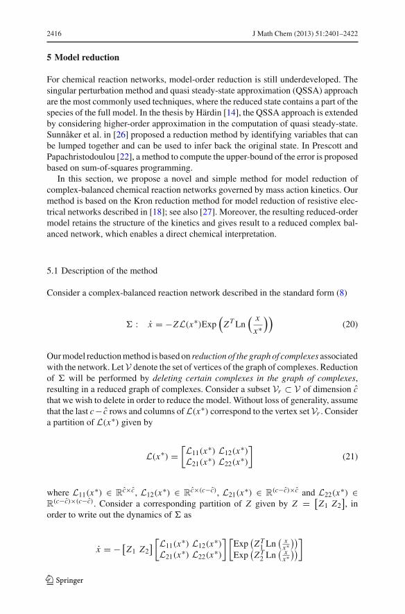
Consider a complex-balanced reaction network described in the standard form (8)

� : x = −ZL(x∗)Exp(

Z T Ln( x

x∗))

(20)

Our model reduction method is based on reduction of the graph of complexes associatedwith the network. Let V denote the set of vertices of the graph of complexes. Reductionof � will be performed by deleting certain complexes in the graph of complexes,resulting in a reduced graph of complexes. Consider a subset Vr ⊂ V of dimension cthat we wish to delete in order to reduce the model. Without loss of generality, assumethat the last c− c rows and columns of L(x∗) correspond to the vertex set Vr . Considera partition of L(x∗) given by

L(x∗) =[L11(x∗) L12(x∗)L21(x∗) L22(x∗)

](21)

where L11(x∗) ∈ Rc×c, L12(x∗) ∈ R

c×(c−c), L21(x∗) ∈ R(c−c)×c and L22(x∗) ∈

R(c−c)×(c−c). Consider a corresponding partition of Z given by Z = [

Z1 Z2], in

order to write out the dynamics of � as

x = − [Z1 Z2

] [L11(x∗) L12(x∗)L21(x∗) L22(x∗)

] [Exp

(Z T

1 Ln( x

x∗))

Exp(Z T

2 Ln( x

x∗))

]

123

J Math Chem (2013) 51:2401–2422 2417

Let L(x∗) denote the Schur complement of L(x∗) with respect to the indices corre-sponding to Vr . Consider now the auxiliary dynamical system

[y1y2

]= −

[L11(x∗) L12(x∗)L21(x∗) L22(x∗)

] [w1w2

]

where we impose the constraint y2 = 0. It follows that

w2 = −L22(x∗)−1L21(x∗)w1,

leading to the reduced auxiliary dynamics defined by the Schur complement

y1 = −(L11(x∗) − L12(x∗)L22(x∗)−1L21(x∗))w1 = −L(x∗)w1

Putting back in w1 = Exp(Z T

1 Ln( x

x∗))

, making use of x = Z1 y1 + Z2 y2 = Z1 y1,

we then obtain the reduced network � given by

� : x = −Z L(x∗)Exp(

Z T Ln( x

x∗))

. (22)

where Z := Z1. We now show that L(x∗) obeys all the properties of the weightedLaplacian matrix of a complex-balanced reaction network corresponding to a graphof complexes with vertex set V − Vr .

Proposition 5.1 Consider a complex-balanced network � with dynamics given byEq. (20). With V , Vr and L as defined above, the following properties hold:

1. All diagonal elements of L(x∗) are positive and off-diagonal elements are non-negative.

2. 1Tc L(x∗) = 0 and L(x∗)1c = 0, where c := c − dim(Vr ).

Proof (1) Follows from the proof of [20, Theorem 3.11]; see also [27] for the case ofsymmetric L.

(2) Without loss of generality, assume that the last c − c rows and columns of L(x∗)correspond to the vertex set Vr . Consider a partition of L(x∗) given by (21). Bydefinition,

L(x∗) = L11(x∗) − L12(x∗)L22(x∗)−1L21(x∗)

Since 1Tc L(x∗) = 0, we obtain

1Tc L11(x∗) + 1T

c−cL21(x∗) = 0; 1Tc L12(x∗) + 1T

c−cL22(x∗) = 0

Using the above equations, we get

1Tc L(x∗) = 1T

c

(L11(x∗) − L12(x∗)L22(x∗)−1L21(x∗)) = −1T

c−cL21(x∗)+1T

c−cL22(x∗)L22(x∗)−1L21(x∗) = 0

123

2418 J Math Chem (2013) 51:2401–2422

In a similar way, it can be proved that L(x∗)1c = 0. �We derive the following properties relating � and �.

Proposition 5.2 Consider the complex-balanced reaction network � and its reducedorder model � given by (22). Denote their sets of equilibria by E , respectively E . ThenE ⊆ E .

Proof Let B denote the incidence matrix for � and let c and c denote the number ofcomplexes in � and � respectively. Assume that the graph of complexes is connected;otherwise the same argument can be repeated for every component (linkage class). Itfollows that ker(BT ) = span(1c). Let x∗∗ ∈ E . We show that x∗∗ ∈ E . Let Z andZ denote the complex-stoichiometric matrices of � and � respectively. Let L(x∗)denote the weighted Laplacian of the graph of complexes of � corresponding to anequilibrium x∗. Let L(x∗) denote the Schur complement of L(x∗) corresponding tothe reduced model �.

Since x∗∗ ∈ E , BT Z T Ln(

x∗∗x∗

)= 0. It follows that Z T Ln

(x∗∗x∗

)∈ span(1c).

This implies that Z T Ln(

x∗∗x∗

)∈ span(1c) since the columns of Z form a subset of the

columns of Z . From Proposition 5.1, it now follows that L(x∗)Exp(Z T Ln

(x∗∗x∗

))=0.

Consequently x∗∗ ∈ E . This concludes the proof. �This proves that � is again a complex-balanced chemical reaction network governed

by mass action kinetics, with a reduced number of complexes and with, in general, adifferent set of reactions (edges of the complex graph). An appropriate choice of Vr

will ensure that some of the elements of x have derivative zero in � leading to lessernumber of state variables in � as compared to �.

We now give a chemical interpretation of our reduction scheme. When a complexbalanced chemical reaction network is perturbed from an equilibrium, it has certainspecies reaching their equilibrium much faster than the remaining ones. The principlebehind our model reduction method is to impose the condition that complexes entirelymade up of such species remain at constant concentrations.

5.2 Effect of model reduction

In this section, we show the effect of our model reduction method on two types ofcomplex-balanced networks with a single linkage class. In other words, we give aninterpretation of our reduced model in terms of its corresponding full model for twotypes of networks. Note that deletion of a set of complexes in one linkage class doesnot affect the reactions of the other linkage classes of the network.

Type 1:

Full Network: C1k1�

k−1C2

k2�k−2

C3k3�

k−3· · · kn−1�

k−(n−1)

Cn (23)

Reduced Network: C1

k1k2k−1+k2�k−1k−2k−1+k2

C3k3�

k−3· · · kn−1�

k−(n−1)

Cn (24)

123

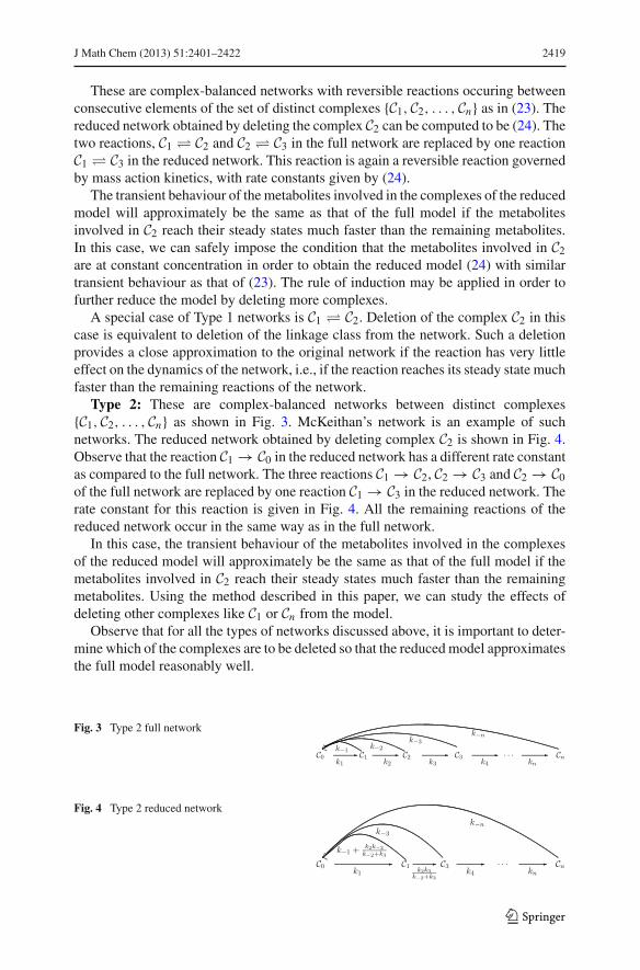
J Math Chem (2013) 51:2401–2422 2419

These are complex-balanced networks with reversible reactions occuring betweenconsecutive elements of the set of distinct complexes {C1, C2, . . . , Cn} as in (23). Thereduced network obtained by deleting the complex C2 can be computed to be (24). Thetwo reactions, C1 � C2 and C2 � C3 in the full network are replaced by one reactionC1 � C3 in the reduced network. This reaction is again a reversible reaction governedby mass action kinetics, with rate constants given by (24).

The transient behaviour of the metabolites involved in the complexes of the reducedmodel will approximately be the same as that of the full model if the metabolitesinvolved in C2 reach their steady states much faster than the remaining metabolites.In this case, we can safely impose the condition that the metabolites involved in C2are at constant concentration in order to obtain the reduced model (24) with similartransient behaviour as that of (23). The rule of induction may be applied in order tofurther reduce the model by deleting more complexes.

A special case of Type 1 networks is C1 � C2. Deletion of the complex C2 in thiscase is equivalent to deletion of the linkage class from the network. Such a deletionprovides a close approximation to the original network if the reaction has very littleeffect on the dynamics of the network, i.e., if the reaction reaches its steady state muchfaster than the remaining reactions of the network.

Type 2: These are complex-balanced networks between distinct complexes{C1, C2, . . . , Cn} as shown in Fig. 3. McKeithan’s network is an example of suchnetworks. The reduced network obtained by deleting complex C2 is shown in Fig. 4.Observe that the reaction C1 → C0 in the reduced network has a different rate constantas compared to the full network. The three reactions C1 → C2, C2 → C3 and C2 → C0of the full network are replaced by one reaction C1 → C3 in the reduced network. Therate constant for this reaction is given in Fig. 4. All the remaining reactions of thereduced network occur in the same way as in the full network.

In this case, the transient behaviour of the metabolites involved in the complexesof the reduced model will approximately be the same as that of the full model if themetabolites involved in C2 reach their steady states much faster than the remainingmetabolites. Using the method described in this paper, we can study the effects ofdeleting other complexes like C1 or Cn from the model.

Observe that for all the types of networks discussed above, it is important to deter-mine which of the complexes are to be deleted so that the reduced model approximatesthe full model reasonably well.

Fig. 3 Type 2 full network

Fig. 4 Type 2 reduced network

123

2420 J Math Chem (2013) 51:2401–2422

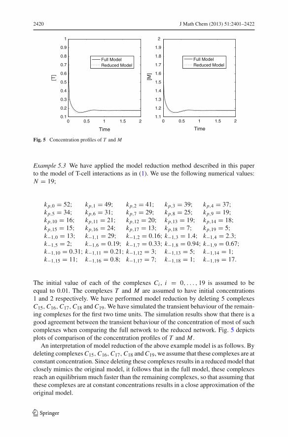
0 0.5 1 1.5 20.1

0.2

0.3

0.4

0.5

0.6

0.7

0.8

0.9

1

Time

[T]

0 0.5 1 1.5 21.1

1.2

1.3

1.4

1.5

1.6

1.7

1.8

1.9

2

Time

[M]

Full ModelReduced Model

Full ModelReduced Model

Fig. 5 Concentration profiles of T and M

Example 5.3 We have applied the model reduction method described in this paperto the model of T-cell interactions as in (1). We use the following numerical values:N = 19;

kp,0 = 52; kp,1 = 49; kp,2 = 41; kp,3 = 39; kp,4 = 37;kp,5 = 34; kp,6 = 31; kp,7 = 29; kp,8 = 25; kp,9 = 19;kp,10 = 16; kp,11 = 21; kp,12 = 20; kp,13 = 19; kp,14 = 18;kp,15 = 15; kp,16 = 24; kp,17 = 13; kp,18 = 7; kp,19 = 5;k−1,0 = 13; k−1,1 = 29; k−1,2 = 0.16; k−1,3 = 1.4; k−1,4 = 2.3;k−1,5 = 2; k−1,6 = 0.19; k−1,7 = 0.33; k−1,8 = 0.94; k−1,9 = 0.67;k−1,10 = 0.31; k−1,11 = 0.21; k−1,12 = 3; k−1,13 = 5; k−1,14 = 1;k−1,15 = 11; k−1,16 = 0.8; k−1,17 = 7; k−1,18 = 1; k−1,19 = 17.

The initial value of each of the complexes Ci , i = 0, . . . , 19 is assumed to beequal to 0.01. The complexes T and M are assumed to have initial concentrations1 and 2 respectively. We have performed model reduction by deleting 5 complexesC15, C16, C17, C18 and C19. We have simulated the transient behaviour of the remain-ing complexes for the first two time units. The simulation results show that there is agood agreement between the transient behaviour of the concentration of most of suchcomplexes when comparing the full network to the reduced network. Fig. 5 depictsplots of comparison of the concentration profiles of T and M .

An interpretation of model reduction of the above example model is as follows. Bydeleting complexes C15, C16, C17, C18 and C19, we assume that these complexes are atconstant concentration. Since deleting these complexes results in a reduced model thatclosely mimics the original model, it follows that in the full model, these complexesreach an equilibrium much faster than the remaining complexes, so that assuming thatthese complexes are at constant concentrations results in a close approximation of theoriginal model.

123

J Math Chem (2013) 51:2401–2422 2421

6 Conclusion

In this paper, we have provided a compact mathematical formulation for the dynamicsof complex-balanced networks. We have made use of this formulation for the determi-nation of equilibria and the asymptotic stability of such networks. The methods thathave been employed are very similar to the ones used in [13], but the difference is thatour proofs are much more concise than the ones presented in [13] due to the use ofproperties of balanced weighted Laplacian matrices of complex-balanced networks.Furthermore, we have made use of the formulation in order to derive a model reductiontechnique for complex-balanced networks.

A main challenge for further research is the extension of our results to chemicalreaction networks with external fluxes and/or externally controlled concentrations.This will change the stability analysis considerably, due to the nonlinearity of thedifferential equations. Furthermore, it will also lead to scrutinizing the model reductiontechnique proposed in this paper from an external (input-output) point of view.

Acknowledgements The research leading to these results has received funding from the Netherlandsorganization for Scientific Research and the European Union Seventh Framework Programme [FP7/2007-2013] under grant agreement No. 257462 HYCON2 Network of Excellence. We thank Anne Shiu for auseful discussion regarding persistence of reaction networks.

References

1. D.F. Anderson, A proof of the global attractor conjecture in the single linkage class case. SIAM J.Appl. Math. 71(4), 1487–1508 (2011)

2. D. Angeli, A tutorial on chemical reaction network dynamics. Eur. J. Control 15(3–4), 398–406 (2009)3. D. Angeli, P. De Leenheer, E.D. Sontag, Graph-theoretic characterizations of monotonicity of chemical

networks in reaction coordinates. J. Math. Biol. 61, 581–616 (2010)4. D. Angeli, P. De Leenheer, E.D. Sontag, Persistence results for chemical reaction networks with time-

dependent kinetics and no global conservation laws. SIAM J. Appl. Math. 71, 128–146 (2011)5. B. Bollobas, Modern Graph Theory,, vol. 184. Graduate Texts in Mathematics (Springer, New York,

1998)6. A. Chapman, M. Mesbahi, Advection on graphs 50th IEEE CDC-ECC (Orlando, USA, 2011), pp.

1461–14667. G. Craciun, M. Feinberg, Multiple equilibria in complex chemical reaction networks: I. The injectivity

property. SIAM J. Appl. Math. 65(5), 1526–1546 (2006)8. G. Craciun, A. Dickenstein, A. Shiu, B. Sturmfels, Toric dynamical systems. J. Symb. Comput. 44,

1551–1565 (2009)9. A. Dickenstein, M.P. Millán, How far is complex balancing from detailed balancing. Bull. Math. Biol.

73, 811–828 (2011)10. F. Dörfler, F. Bullo, Kron reduction of graphs with applications to electrical networks. IEEE Trans.

Circuits Syst. I 99, 1–14 (2012)11. M. Feinberg, Complex balancing in chemical kinetics. Arch. Ration. Mech. Anal. 49, 187–194 (1972)12. M. Feinberg, Chemical reaction network structure and the stability of complex isothermal reactors -I.

The deficiency zero and deficiency one theorems. Chem. Eng. Sci. 43(10), 2229–2268 (1987)13. M. Feinberg, The existence and uniqueness of steady states for a class of chemical reaction networks.

Arch. Ration. Mech. Anal. 132, 311–370 (1995)14. H.M. Härdin, Handling Biological Complexity: As Simple as Possible but not Simpler. Ph.D. Thesis,

(Vrije Universiteit Amsterdam, 2010)15. F.J.M. Horn, Necessary and sufficient conditions for complex balancing in chemical kinetics. Arch.

Ration. Mech. Anal. 49, 172–186 (1972)16. F. Horn, R. Jackson, General mass action kinetics. Arch. Ration. Mech. Anal. 47, 81–116 (1972)

123

2422 J Math Chem (2013) 51:2401–2422

17. B. Jayawardhana, S. Rao, A. van der Schaft, Balanced chemical reaction networks governed by generalkinetics. in Proceedings fo 20th Mathematical Theory of Networks and Systems, Melbourne, June(2012)

18. G. Kron, Tensor Analysis of Networks (Wiley, New York, 1939)19. T.W. McKeithan, Kinetic proofreading in T-cell receptor signal transduction. Proc. Natl. Acad. Sci.

USA 92, 5042–5046 (1995)20. N.M.D. Niezink, Consensus in Networked Multi-agent Systems. Master’s thesis in Applied Mathemat-

ics (Faculty of Mathematics and Natural Sciences, University of Groningen, August 2011)21. H.G. Othmer, Analysis of Complex Reaction Networks. Lecture Notes, (School of Mathematics, Uni-

versity of Minnesota, 9 December, 2003)22. T.P. Prescott, A. Papachristodoulou, Guaranteed error bounds for structured complexity reduction of

biochemical networks. J. Theor. Biol. 304, 172–182 (2012)23. S. Rao, B. Jayawardhana, A.J. van der Schaft, On the graph and systems analysis of reversible chemical

reaction networks with mass action kinetics. Proc. IEEE Am. Control Conf., Montreal, June 201224. D. Siegel, D. MacLean, Global stability of complex balanced mechanisms. J. Math. Chem. 27, 89–110

(2000)25. E.D. Sontag, Structure and stability of certain chemical networks and applications to the kinetic proof-

reading model of T-cell receptor signal transduction. IEEE Trans. Autom. Control 46(7), 1028–1047(2001)

26. M. Sunnåker, G. Cedersund, M. Jirstrand, A method for zooming of nonlinear models of biochemicalsystems. BMC Syst. Biol. 5, 140 (2011)

27. A.J. van der Schaft, Characterization and partial synthesis of the behavior of resistive circuits at theirterminals. Syst. Control Lett. 59, 423–428 (2010)

28. A.J. van der Schaft, S. Rao, B. Jayawardhana, On the mathematical structure of balanced chemicalreaction networks governed by mass action kinetics. SIAM J. Appl. Math. 73(2), 953–973 (2013)

123