1

A Survey of Graph Theoretical Approaches to Image Segmentation

Bo Penga,b, Lei Zhangb,1, and David Zhangb

a Dept. of Software Engineering, Southwest Jiaotong University, Chengdu, China bDept. of Computing, The Hong Kong Polytechnic University, Kowloon, Hong Kong, China

Abstract: Image segmentation is a fundamental problem in computer vision. Despite many years of

research, general purpose image segmentation is still a very challenging task because segmentation is

inherently ill-posed. Among different segmentation schemes, graph theoretical ones have several good

features in practical applications. It explicitly organizes the image elements into mathematically sound

structures, and makes the formulation of the problem more flexible and the computation more

efficient. In this paper, we conduct a systematic survey of graph theoretical methods for image

segmentation, where the problem is modeled in terms of partitioning a graph into several sub-graphs

such that each of them represents a meaningful object of interest in the image. These methods are

categorized into five classes under a uniform notation: the minimal spanning tree based methods,

graph cut based methods with cost functions, graph cut based methods on Markov random field

models, the shortest path based methods and the other methods that do not belong to any of these

classes. We present motivations and detailed technical descriptions for each category of methods. The

quantitative evaluation is carried by using five indices – Probabilistic Rand (PR) index, Normalized

Probabilistic Rand (NPR) index, Variation of Information (VI), Global Consistency Error (GCE) and

Boundary Displacement Error (BDE) – on some representative automatic and interactive

segmentation methods.

Keywords: image segmentation, graph theoretical methods, minimal spanning tree, graph cut

1 Corresponding author. Email: cslzhang@comp.polyu.edu.hk.

2

1. Introduction

Image segmentation is a classical and fundamental problem in computer vision. It refers to

partitioning an image into several disjoint subsets such that each subset corresponds to a meaningful

part of the image. As an integral step of many computer vision problems, the quality of segmentation

output largely influences the performance of the whole vision system. A rich amount of literature on

image segmentation has been published over the past decades. Some of them have achieved an

extraordinary success and become popular in a wide range of applications, such as medical image

processing [1-3], object tracking [4-5], recognition [6-7], image reconstruction [8-9] and so on.

Since the very beginning, image segmentation has been closely related to perceptual grouping or

data clustering. Such a relationship was clearly pointed out by Wertheimer’s gestalt theory [10] in

1938. In this theory, a set of grouping laws such as similarity, proximity and good continuation are

identified to explain the particular way by which the human perceptual system groups tokens together.

The gestalt theory has inspired many approaches to segmentation, and it is hoped that a good

segmentation can capture perceptually important clusters which reflect local and/or global properties

of the image. Early edge detection methods such as the Robert edge detector, the Sobel edge detector

[11] and the Canny edge detector [12-13] are based on the abrupt changes in image intensity or color.

Due to the distinguishable features of the objects and the background, a large number of thresholding

based methods [14-16] have been proposed to separate the objects from the background. In the partial

differential equations (PDE) based methods [17-18, 19-21], the segmentation of a given image is

calculated by evolving parametric curves in the continuous space such that an energy functional is

minimized for a desirable segmentation. Region splitting and merging is another popular category of

segmentation methods, where the segmentation is performed in an iterative manner until some

uniformity criteria [22-23] are satisfied. The reviews of various segmentation techniques can be found

for image thresholding methods [24], medical image segmentation [25-26], statistical level set

segmentation [27], 3D image segmentation [28], edge detection techniques [29] and so on.

Among the previous image segmentation techniques, many successful ones benefit from mapping

the image elements onto a graph. The segmentation problem is then solved in a spatially discrete

3

space by the efficient tools from graph theory. One of the advantages of formulating the segmentation

on a graph is that it might require no discretization by virtue of purely combinatorial operators and

thus incur no discretization errors. Despite the large amount of efforts devoted to image segmentation,

little work has been done to review the work in this field. In this paper, we conduct a systematic

survey of some influential graph theoretic techniques for image segmentation, where the problem is

generally modeled in term of partitioning a graph into several sub-graphs.

With a history dating back to 1960s, the earliest graph theoretic methods stress the importance of

the gestalt principles of similarity or proximity in capturing perceptual clusters. The graph is then

partitioned according to these criteria such that each partition is considered as an object segment in

the image. In these methods, fixed thresholds and local measures are usually used for computing the

segmentation results, while global properties of segmentation are hard to guarantee. The introduction

of graph as a general approach to segmentation with a global cost function was brought by Wu et al.

[30] in 1990s. From then on, much research attention was moved to the study of optimization

techniques on the graph. It is known that one of the difficulties in image segmentation is its ill-posed

nature. Since there are multiple possible interpretations of the image content, it might be difficult to

find a single correct answer for segmenting a given image. This suggests that image segmentation

should incorporate the mid- and high-level knowledge in order to accurately extract objects of interest.

In the late 1990s, a prominent graph technique emerged in the use of a combination of model-specific

cues and contextual information. An influential representation is the s/t graph cut algorithm [31]. Its

technical framework is closely related to some variational methods [17-18, 19-21] in terms of a

discrete manner. Up to now, s/t graph cut and its variants have been extended for solving many

computer vision problems, and eventually acting as an optimization tool in these areas.

This paper provides a systematic survey of graph theoretic techniques and distinguishes them by

broadly grouping them into five categories. (1) Minimal spanning tree based methods: the clustering

or grouping of image pixels are performed on the minimal spanning tree. The connection of graph

vertices satisfies the minimal sum on the defined edge weights, and the partition of a graph is

achieved by removing edges to form different sub-graphs. (2) Graph cut with cost functions: graph cut

is a natural description of image segmentation. Using different cut criteria, the global functions for

4

partitioning the graph will be different. Usually, by optimizing these functions, we can get the

desirable segmentation. (3) Graph cut on Markov random field models: the goal is to combine the

high level interactive information with the regularization of the smoothness in the graph cut function.

Under the MAP-MRF framework, the optimization of the function is obtained by the classical min-

cut/max-flow algorithms or its nearly optimal variants. (4) The shortest path based methods: the

object boundary is defined on a set of shortest path between pairs of graph vertices. These methods

require user interactions to guide the segmentation. Therefore, the process is more flexible and can

provide friendly feedback. (5) Other methods: we will refer to several efficient graph theoretic

methods that do not belong to any of the above categories, such as random walker [32] and dominant

set based method [33].

For each of the above categories, the principle of graph theory will be firstly introduced, and then

the theoretic formulation as well as their segmentation criteria will be reviewed. Performance

assessment of some well-known methods will also be given for the sake of completeness and

illustration. The outline of the paper is as follows. In Section 2, important notations and definitions in

graph theory are introduced. In Section 3, the methodologies of the five categories of methods are

reviewed. Explicit explanations are presented on the formulation of the problem and the details of

different segmentation criteria. In Section 4, some quantitative metrics of the segmentation quality are

described. The performances of some representative automatic and interactive segmentation

techniques are analyzed in Section 5 and Section 6, respectively. In Section 7, the applications of

graph based methods in medical image segmentation are discussed. Section 8 draws the conclusion.

2. Background

In this section we define some terminologies that will be used throughout the paper for explaining the

graph based segmentation methods.

Let G = (V, E) be a graph where V ={ v1 ,..., vn } is a set of vertices corresponding to the image

elements, which might represent pixels or regions in the Euclidean space. E is a set of edges

connecting certain pairs of neighboring vertices. Each edge (vi,vj)∈E has a corresponding weight

5

w(vi,vj) which measures a certain quantity based on the property between the two vertices connected

by that edge. For image segmentation, an image is partitioned into mutually exclusive components,

such that each component A is a connected graph G′=(V′, E′), where V′⊆ V, E′⊆ E and E' contains

only edges built from the nodes of V'. In other words, nonempty sets A1, …, Ak form a partition of the

graph G if Ai∩Aj =φ (i,j∈{1, 2, …, k}, i≠j) and A1∪…∪Ak=G. The well-accepted segmentation criteria

[10] require that image elements in each component should have uniform and homogeneous

properties in the form of brightness, color, or texture, etc., and elements in different components

should be dissimilar.

In graph theoretic definition, the degree of dissimilarity between two components can be

computed in the form of a graph cut. A cut is related to a set of edges by which the graph G will be

partitioned into two disjoint sets A and B. As a consequence, the segmentation of an image can be

interpreted in form of graph cuts, and the cut value is usually defined as:

∑ ∈∈=

BvAuvuwBAcut

,),(),( (1)

where u and v refer to the vertices in the two different components. In image segmentation, noise and

other ambiguities bring uncertainties into the understanding of image content. The exact solution to

image segmentation is hard to obtain. Therefore, it is more appropriate to solve this problem with

optimization methods. The optimization-based approach formulates the problem as a minimization of

some established criterion, whereas one can find an exact or approximate solution to the original

uncertain visual problem. In this case, the optimal bi-partitioning of a graph can be taken as the one

which minimizes the cut value in Eq. (1).

In a large amount of literature, image segmentation is also formulated as a labeling problem,

where a set of labels L is assigned to a set of sites in S. In two-class segmentation, for example, the

problem can be described as assigning a label fi from the set L={object, background} to site i∈S

where the elements in S are the image pixels or regions. Labeling can be performed separately from

image partitioning, while they achieve the same effect on image segmentation. We will see in this

survey that many methods perform both partitioning and labeling simultaneously. An example to

illustrate the relationship between graph cuts and the corresponding vertex labeling is given in Fig. 1,

6

where a graph is segmented by two cuts and thus has 3 labels in the final segmentation.

(a) Graph cuts (b) A labeling

Figure 1: An example of graph cuts and the corresponding vertex labeling. (a) shows a graph whose vertices are image pixels, and maintains the 4-neighborhood system. Graph cuts separate the graph into three subgraphs. A labeling shown in (b) assigns some label Lp∈{0,1,2} to each pixel w.r.t. the graph cuts. Thick lines show labeling discontinuities between neighboring pixels.

Methods in image segmentation can be categorized into automatic methods and interactive

methods. Automatic segmentation is desirable in many cases for its convenience and generality.

However, in many applications such as medical or biomedical imaging, objects of interest are often

ill-defined so that even sophisticated automatic segmentation algorithms will fail. Interactive methods

can improve the accuracy by incorporating prior knowledge from the user; however, in some practical

applications where a large number of images are needed to be handled, they can be laborious and time

consuming. Note that automatic and interactive methods are often used together to improve the

segmentation results. Some automatic segmentation methods may require interaction for setting initial

parameters and some interactive methods may start with the results from automatic segmentation as

an initial segmentation. In this survey, the methods we will introduce refer to either of the two

categories.

3. Methods

In this section, we review the representative methods on graph based image segmentation. For each

class of methods, we provide the formulation of the problem and present an overview of how the

methods are implemented. The advantages and disadvantages of these methods are discussed as well.

7

Although we classify the methods into five categories, some of them are often used in conjunction

with one another. The main differences between these methods lie in how they define the desirable

quality in the segmentation and how they achieve it using distinctive graph properties.

3.1 Minimal spanning tree (MST) based methods

The minimal spanning tree (MST) (also called shortest spanning tree) is an important concept in graph

theory. A spanning tree T of a graph G is a tree such that T = (V, E′), where E′⊆ E. A graph may have

several different spanning trees. The MST is then a spanning tree with the smallest weights among all

spanning trees. The algorithms for computing the MST can be found in [34-36]. For example, in

Prim’s algorithm [36], the MST is constructed by iteratively adding the frontier edge of the smallest

edge-weight. The algorithm is in a greedy style and runs in polynomial time.

MST based segmentation methods are essentially related to the graph based clustering. The

general study of graph clustering can be dated back to 1970s or earlier. In graph based clustering, the

data to be clustered are represented by an undirected adjacency graph. To represent the affinity, edges

with certain weights are defined between two vertices if they are neighbors according to a given

neighborhood system. Clustering is then achieved by removing edges of the graph to form mutually

exclusive subgraphs. The clustering process usually emphasizes the importance of the gestalt

principles of similarity or proximity in the graph vertices.

The early MST based methods [37] perform image segmentation in an implicit way, which is

based on the inherent relationship between the MST and cluster structure. The intuition underlying

this relationship is that the MST consists of edges with the minimal sum of weights among all

spanning trees, and as a result, it guarantees the connection of graph vertices which are most similar to

each other (i.e., at the lowest cost of weights). This nature makes MST spans all the vertices and at the

same time jump across the smaller gaps between different clusters. However, it is not enough to deal

with situations when there is a large variation inside a cluster. The complex scenes in real world

images often have perceptually meaningful clusters with non-uniform densities; therefore it is more

desirable to consider both the difference across the two clusters and the difference inside a cluster. The

8

gestalt principles play an important role in guiding the MST based image segmentation; however,

there lacks a precise measurement on the definition in the quantitative results.

Morris et al. [38] used MST to hierarchically partition images. Their method can obtain the

segmentation in different scales based on the principle that the most similar pixels should be grouped

together and dissimilar pixels should be separated. By cutting the MST at the highest edge weights,

partitions of a graph are formed with the maximal difference between neighboring sub-graphs. In [38],

some improved algorithms were also proposed based on MST, e.g., the recursive MST algorithm. In

each iteration, the segmentation is formed by partitioning one sub-graph. Therefore, the algorithm can

lead to a final segmentation with a given number of sub-graphs. Apparently, the algorithm in this form

is inefficient. Kwok et al. [39] proposed a fast recursive MST algorithm to speed up Morris et al.’s

method.

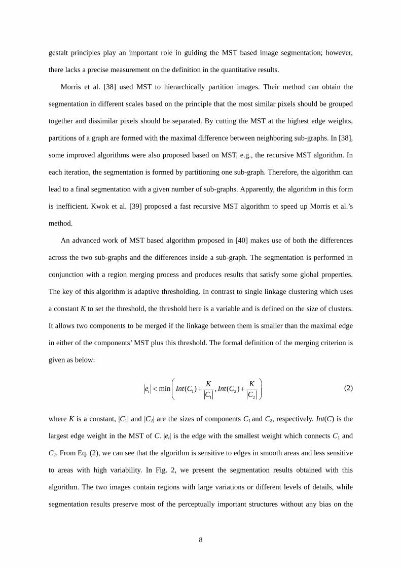
An advanced work of MST based algorithm proposed in [40] makes use of both the differences

across the two sub-graphs and the differences inside a sub-graph. The segmentation is performed in

conjunction with a region merging process and produces results that satisfy some global properties.

The key of this algorithm is adaptive thresholding. In contrast to single linkage clustering which uses

a constant K to set the threshold, the threshold here is a variable and is defined on the size of clusters.

It allows two components to be merged if the linkage between them is smaller than the maximal edge

in either of the components’ MST plus this threshold. The formal definition of the merging criterion is

given as below:

1 21 2

min ( ) , ( )tK Ke Int C Int CC C

⎛ ⎞< + +⎜ ⎟⎜ ⎟

⎝ ⎠ (2)

where K is a constant, |C1| and |C2| are the sizes of components C1 and C2, respectively. Int(C) is the

largest edge weight in the MST of C. |et| is the edge with the smallest weight which connects C1 and

C2. From Eq. (2), we can see that the algorithm is sensitive to edges in smooth areas and less sensitive

to areas with high variability. In Fig. 2, we present the segmentation results obtained with this

algorithm. The two images contain regions with large variations or different levels of details, while

segmentation results preserve most of the perceptually important structures without any bias on the

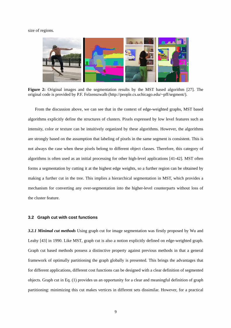
9

size of regions.

Figure 2: Original images and the segmentation results by the MST based algorithm [27]. The original code is provided by P.F. Felzenszwalb (http://people.cs.uchicago.edu/~pff/segment/).

From the discussion above, we can see that in the context of edge-weighted graphs, MST based

algorithms explicitly define the structures of clusters. Pixels expressed by low level features such as

intensity, color or texture can be intuitively organized by these algorithms. However, the algorithms

are strongly based on the assumption that labeling of pixels in the same segment is consistent. This is

not always the case when these pixels belong to different object classes. Therefore, this category of

algorithms is often used as an initial processing for other high-level applications [41-42]. MST often

forms a segmentation by cutting it at the highest edge weights, so a further region can be obtained by

making a further cut in the tree. This implies a hierarchical segmentation in MST, which provides a

mechanism for converting any over-segmentation into the higher-level counterparts without loss of

the cluster feature.

3.2 Graph cut with cost functions

3.2.1 Minimal cut methods Using graph cut for image segmentation was firstly proposed by Wu and

Leahy [43] in 1990. Like MST, graph cut is also a notion explicitly defined on edge-weighted graph.

Graph cut based methods possess a distinctive property against previous methods in that a general

framework of optimally partitioning the graph globally is presented. This brings the advantages that

for different applications, different cost functions can be designed with a clear definition of segmented

objects. Graph cut in Eq. (1) provides us an opportunity for a clear and meaningful definition of graph

partitioning: minimizing this cut makes vertices in different sets dissimilar. However, for a practical

10

graph partition problem, it also requires vertices in the same set to be similar. These two requirements

are studied by existing graph cut methods, which attempt to satisfy one or two of the requirements.

In Wu and Leahy’s work [43], they minimized a cost function formulated exactly in the form of

Eq. (1), namely minimal cut. According to the Ford-Fulkerson theorem [44], the maximum flow

between a pair of vertices equals to the value of the minimal s/t-cut, which could be solved efficiently.

In [43], the authors also discussed a more general case where a k-partition of graph G is identified by

using the Gomory-Hu algorithm [45], as an equivalent of “finding the maximal flow between k-pairs

of vertices”.

3.2.2. Normalized cut methods The minimal cut criterion is intuitive to illustrate the idea of gestalt

principle; however, it has a bias toward finding small components. To alleviate this problem, one

should consider to explicitly require that each individual set is “reasonably large”. Several studies

have been done to address this problem, which lead to various normalized objective functions.

One well-known objective function to avoid this unnatural bias is proposed by Shi et al. [46] in

terms of normalized cut (Ncut). The graph cut is measured by the weights of vol(⋅), which is the total

connection from vertices in a set (e.g., A) to all the vertices in the graph. Formally we have

∑ ∈∈= VjvAiv ji vvwAvol , ),()( , where weight w(vi,vj) measures a certain image quantity (e.g., intensity,

color, etc.) between the two vertices connected by that edge. Then Ncut cost function is defined as

follows:

∑

∑

∑

∑

<

><

>

<> −+

−=

+=

0

)0,0(

0

)0,0( ),(),(

)(),(

)(),(),(Ncut

ix i

jxix jiji

ix i

jxix jiji

dxxvvw

dxxvvw

BvolBAcut

AvolBAcutBA

(3)

where xi is the indicator variable, xi = 1 if vertex vi is in A and xi = -1 otherwise. ∑= j jii vvwd ),( is

the total connection from vi to all the other vertices. Note that with this definition, the partitions

containing small set of vertices will not have small Ncut value, and hence the minimal cut bias is

circumvented. The minimization of Eq. (3) can be formulated into a generalized eigenvalue problem,

which has been well-studied in the field of spectral graph theory. After a common matrix

11

transformation, the Ncut problem can be re-written into:

( )min Ncut( , ) minT

TA B −= y

y D W yy Dy

(4)

subject to y(i)∈{1,-b}, ∑

∑

<

>=0

0

ix i

ix i

dd

b and yTD1=0, where D and W are the degree matrix and the

adjacency matrix of G, respectively. We call L=D-W the graph Laplacian of G. It can be seen that -b

represents the ratio of connections which are from vi to vertices inside and outside the same set,

respectively. The relaxed optimization of Eq. (4) is obtained by discarding the discreteness condition

but allowing y to take arbitrary real values. According to the Rayleigh-Ritz theorem [47], the

eigenvector corresponding to the second smallest general eigenvalue of L is the real valued solution to

the relaxed version of Eq. (4). Finally, to partition the graph, one can perform a simple thresholding

on this eigenvector. The multi-class partitioning is also discussed in [46], where an iterative process of

2-way partition is implemented on the graph until a satisfactory result is achieved. Fig. 3 shows a

segmentation example of Ncut, where the Figs. 3 (c-h) are the eigenvectors corresponding to the

second smallest to the seventh smallest eigenvalues of the system. Partitioning the graph into 6 pieces

using the second smallest eigenvector, we obtain the segmentation result in Fig. 3(b).

(a) (b) (c) (d)

(e) (f) (g) (h)

Figure 3: (a) The original image. (b) The segmentation result of Ncut algorithm [46]. (c-h) The eigenvectors corresponding to the second smallest to the seventh smallest eigenvalues of the system. The eigenvectors are reshaped to be the size of the image. The code is provided by Shi et al. [46] (http://www.cis.upenn.edu/~jshi/software/).

In fact, not limited to image segmentation, there has been several existing works in spectral graph

12

clustering referring to the “graph cut” problem. The ratio cut [48] and MinMaxCut [49] define

different cut functions on other types of data and lead to different graph Laplacians for clustering.

These methods all overcome the drawback of Wu et al’s minimal cut criterion and achieve “balanced”

partitions. As a clustering method, spectral clustering often outperforms the traditional approaches in

its efficiency and simplicity in implementation.

Cox et al. [50] incorporated the interior region and boundary information in image segmentation.

To this end, the ratio between the exterior boundary cost and the enclosed interior benefit is

minimized using an efficient graph partitioning algorithm. Let P be a directed path in G that starts and

finishes at the same node v. Denote by cost(P) the length of the boundary, and by weight(P) the

segment-area cost. The graph cut cost function is then defined as:

( )Regioncut( , )( )

cost PA Bweight P

= (5)

Obviously, this cut criterion favorites large objects in the image and the object characteristic of

smoothness is induced via the area and perimeter measures. This definition is very similar to Eq. (3)

except that it is defined on a single region. Additionally, one can use different interior information

such as the intensity, texture or the size of the region in coding the area term. The limitation of this

method is that it can only segment enclosed objects due to the definition of cost function.

The mean cut [51] proposed by Wang et al. addresses the problem by defining an edge-weight

function:

)1|,()),(|,(),(Meancut

BAcutvuwBAcutBA = (6)

where cut(A,B|w(u,v)) is the cut cost between region A and region B given the edge weight w(u,v),

cut(A,B|1) is defined similarly with all edge weights to be 1. This cut function minimizes the average

edge weight in the cut boundary. It allows both open and closed boundaries and guarantees that

partitions are connected. However, the mean cut criterion does not explicitly introduce the bias on the

preference for large object regions or smooth boundaries. The authors argued that this lack of bias

allows producing segmentations that are better aligned with image edges. The global minimization is

13

performed in a polynomial time by graph theoretic algorithm, but limited to connected planar graphs.

To solve the cost function Eq. (6), there are three reductions in their algorithm: from minimal mean

cut to minimal mean simple cycle, from minimal mean simple cycle to negative simple cycle, and

from negative simple cycle to minimal weight perfect matching. Afterwards Wang and Siskind

extended the mean cut to a more general form called ratio cut [52]. The ratio cut inherits the merit of

mean cut but corresponds to the average affinity per unit length of the segmentation boundary instead

of the average affinity per element of the cut boundary. Furthermore, graph nodes in ratio cut method

correspond to regions which are created by iterated region-based segmentation. The cut function is

formulated as:

1

2

( , )Rcut( , )( , )

cut A BA Bcut A B

= (7)

where cut1(A,B) and cut2(A,B) are defined on the graphs of different iterations. Mean cut is the same

as ratio cut when cut2(A,B) contains the unit weights. Minimization of ratio cut for arbitrary graph is

NP-hard, and thus the same reduction process is used as in the mean cut.

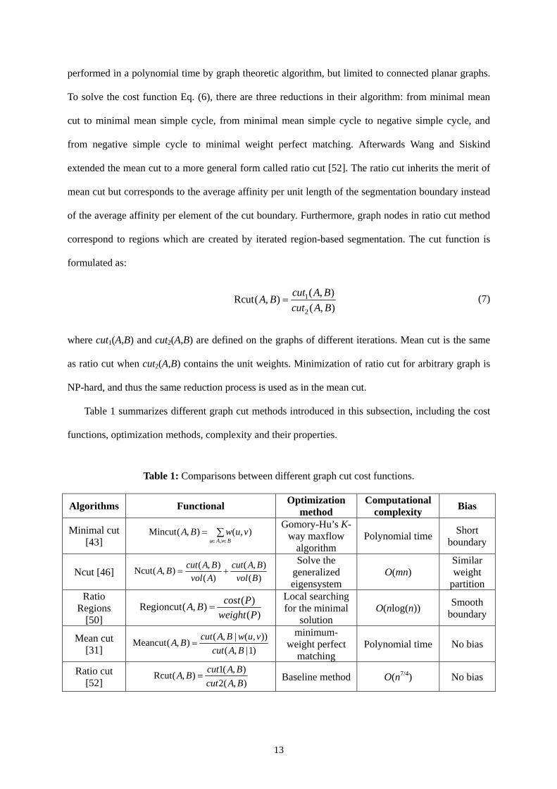
Table 1 summarizes different graph cut methods introduced in this subsection, including the cost

functions, optimization methods, complexity and their properties.

Table 1: Comparisons between different graph cut cost functions.

Algorithms Functional Optimization method

Computational complexity Bias

Minimal cut [43]

∑∈∈

=BvAu

vuwBA,

),(),(Mincut Gomory-Hu’s K-

way maxflow algorithm

Polynomial time Short boundary

Ncut [46] )(),(

)(),(),(Ncut

BvolBAcut

AvolBAcutBA +=

Solve the generalized eigensystem

O(mn) Similar weight

partition Ratio

Regions [50]

( )Regioncut( , )( )

cost PA Bweight P

= Local searching for the minimal

solution O(nlog(n)) Smooth

boundary

Mean cut [31] )1|,(

)),(|,(),(MeancutBAcut

vuwBAcutBA =minimum-

weight perfect matching

Polynomial time No bias

Ratio cut [52] ),(2

),(1),(RcutBAcutBAcutBA = Baseline method O(n7/4) No bias

14

Graph cut methods provide well-defined relationship between the segments, while the problem of

finding a cut in an arbitrary graph may be NP-hard. Efficient approximation of the solution needs to

be studied. Since these methods form good basis for general image segmentation problem, they can be

combined with other segmentation techniques for further extension.

3.3 Graph cut on Markov random field models

The study of psychology suggests that the use of contextual constraints is crucial for interpreting

visual information. For example, an image should be understood in both of the spatial and visual

contexts. The Markov random field (MRF) theory provides a useful and consistent way of modeling

contextual information such as image pixels and features. In this framework, the mutual influences

among pixels can be formulated into conditional MRF distributions. Due to the equivalence between

MRF’s and Gibbs distributions, a mathematically sound means is built for transforming the joint

distribution of an MRF into a simple form. In conjunction with the Bayesian maximum a posterior

(MAP) estimation, the MAP-MRF framework [53-56] formulates the labeling problem into a problem

of minimizing an energy function: f*=argminfE(f|d), where d is the observation of image elements, f is

the unknown labeling, and E(f|d) is thus the posterior energy function. Compared with the graph cut

methods introduced in Section 3.2.1, the methods discussed in this section will emphasize on the

MAP-MRF framework which tends to explicitly incorporate any desirable high-level contextual

information in the energy function.

3.3.1 Bi-labeling graph cut (s/t graph cut) methods Strategies for optimizing the energy functional

can be various. For those defined on discrete set of variables, the combinatorial min-cut/max-flow

graph cut algorithm [57] is a prominent one. Greig et al. [58] are the first to find out that powerful

min-cut/max-flow algorithms can be used to minimize certain energy functions in image restoration.

The energy functional they used is:

∑ ∑∈ ∈

+=Pp Nqp

qpqppp ffVfDfE),(

, ),()()( λ (8)

where fp is the label of an image pixel, Dp(⋅) is the regional term that measures the penalties for

15

assigning fp to p, Vp,q(⋅) is the boundary term for measuring the interaction potential, and N is the

neighborhood set. This graph energy functional is later brought attention in multi-camera stereo

problem [59] and further generalized to image segmentation for convex or non-convex problems.

The graph cut energy functional encodes both the constraints from user interaction and the

regularization of the image smoothness under the MAP-MRF framework. In the graph cut model,

edges E consist of two types of links to formulate these two constraints: t-links and n-links. Visual

terminal nodes are added in the graph to represent the user input information. For example, if one

attempts to partition an image into two classes (i.e., the object and the background), the class

information is then modeled as two visual terminal nodes based on the user input. With this setting,

each node is connected to the terminal nodes by t-links, and each pair of neighboring nodes is

connected by an n-link. The relationship between the energy functional and a graph cut model is

illustrated in Fig. 4, where the boundary term and the regional term of Eq. (8) define the n-links and t-

links in the graph, respectively. Fig. 4(a) shows an example of bi-labeling cut and Fig. 4(b) shows

graph cut with multi-labels. Some of the t-links are omitted for the convenience of illustration.

(a) 2-way cut (b) multi-way cut

Figure 4: Graph cut model and labeling for a 3×3 image. (a) An s/t graph cut model (left), where the boundary term in Eq. (8) defines the n-links and the regional term defines the t-links. A cut partitions the graph into two sets (right). (b) A multi-label graph cut model (left) and a multiway cut (right).

The work in [60] studies what energy functionals can be minimized via graph cut. In particular, it

provides a simple necessary and sufficient condition on energy functionals of binary variables with

double and triple cliques. The global optimal solution of minimal cut can be found by different

combinatorial min-cut/max-flow algorithms [44,61-64], where Boykov and Kolmogorov’s

augmenting-path based algorithm [62] has the best performance for common vision problems. For

huge 2D or 3D grids, the parallelizing of graph cut algorithm has also been studied [65-66, 67]. Fig. 5

16

demonstrates some examples of image segmentation by s/t graph cut.

Figure 5: Examples of s/t graph cut segmentation, where user interactively inputs objects seeds (red strokes) and background seeds (green strokes).

The most typical way to represent the object/background models is based on the intensity

distributions (e.g., histogram). Blake et al. [68] suggested using a Gaussian Mixture model (GMM) to

approximate the distributions. As the object/background models are updated interactively, the high-

level contextual information is enhanced for a stable representation of the objects of interest. A similar

way of iteratively updating the regional term was proposed in [69], where the information is obtained

progressively from the local image. In each iteration, only the local neighboring regions to the labeled

regions are involved in the optimization so that much interference from the far unknown regions can

be significantly reduced. Fig. 6 shows an example of segmentation with this method.

Figure 6: The iterated segmentation process of [69]. From left to right and top to bottom: user input seeds and initial segmentation by watershed method [70]; the intermediate segmentation results in the 1st, 2nd and 3rd iterations; the segmentation result; and the energy evolution of this process. The newly added regions in the sub-graphs are shown in red color and the background regions are in blue color. We can see that the target object is well segmented from the background. The graph cut energy decreases monotonically in the iterated process.

The boundary term of Eq. (8) reflects the smoothness of the segmentation, and hence the penalty

17

of neighboring graph elements will be small if they are similar. To describe such a penalty, local

intensity gradient or color histograms are the most commonly used criteria. Boykov et al. [71]

investigated geometric properties of segments. They showed that discrete topology of graph cut can

approximate any continuous Riemannian metric space. Thus many of the well-known geometric

methods based on level sets [18, 72] can also be studied in the discrete space by the combinatorial

graph cut.

3.3.2 Multi-labeling graph cut methods The standard s/t graph cut algorithm can find the exact

optimal solution for a certain class of energy functionals [60]; however, in many cases the number of

labels for assigning to graph nodes is more than two, and the minimization of energy functions

becomes NP-hard. For approximate optimization, Boykov et al. [31] developed the α-expansion-

move and αβ-swap-move algorithms to deal with multi-labeling problems for more general energy

functionals. Although the algorithms can only find local minimum solutions, their effectiveness has

been validated by extensive experiments. This work inspires more studies to incorporate various

constraints in the energy functional. In [73-75], the authors used ordering constraints in object

segmentation. By defining the spatial relationship between the objects, the impossible segmentation is

ruled out. The improved α-expansion-move algorithms make the optimization of energy functional

more effective under the constraints.

3.3.3 Graph cut with shape prior Incorporating the shape prior in graph cut has been proven very

useful for image segmentation. This visual cue can be added in either the regional term or the

boundary terms to force the segmented object to follow a certain pre-defined shape. The idea of using

a signed distance map function to represent some shape was proposed by Kolmogorov and Boykov

[60], where they pointed out that combining geometric concept of flux and length/area in the regional

term can improve the segmentation quality of long thin objects. In [76], the gradient flow evolution of

a surface was computed by the L2 distance of the drifting from its current position. It guarantees that

the shape is not very far from the previous position in the evolving process. Freedman et al. [77] used

a similar idea as in level-sets [21, 78] to specify the template as a distance function whose zero level

18

set corresponds to the template. The rigid and the scale transformations were also considered in this

work, where the shape term is integrated into the boundary term of the energy functional. Instead of

using the specific shape template, Das et al. [79] and Veksler [80] studied more generic shape priors

for image segmentation. These shapes are defined on the relative positions of neighboring pixel pairs,

thus the neighborhood system for incorporating the shape constraints is the same as for the boundary

constraints. In 2-labeling case, minimizing the shape based energy functionals can be accomplished

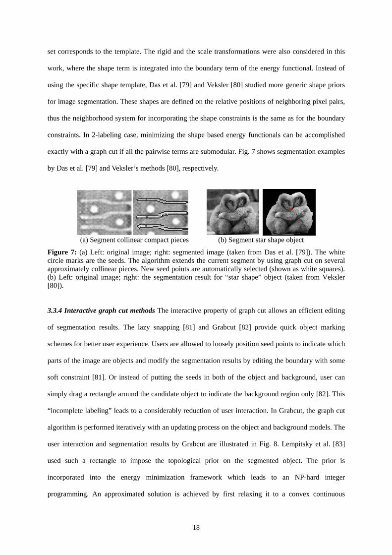
exactly with a graph cut if all the pairwise terms are submodular. Fig. 7 shows segmentation examples

by Das et al. [79] and Veksler’s methods [80], respectively.

(a) Segment collinear compact pieces (b) Segment star shape object

Figure 7: (a) Left: original image; right: segmented image (taken from Das et al. [79]). The white circle marks are the seeds. The algorithm extends the current segment by using graph cut on several approximately collinear pieces. New seed points are automatically selected (shown as white squares). (b) Left: original image; right: the segmentation result for “star shape” object (taken from Veksler [80]).

3.3.4 Interactive graph cut methods The interactive property of graph cut allows an efficient editing

of segmentation results. The lazy snapping [81] and Grabcut [82] provide quick object marking

schemes for better user experience. Users are allowed to loosely position seed points to indicate which

parts of the image are objects and modify the segmentation results by editing the boundary with some

soft constraint [81]. Or instead of putting the seeds in both of the object and background, user can

simply drag a rectangle around the candidate object to indicate the background region only [82]. This

“incomplete labeling” leads to a considerably reduction of user interaction. In Grabcut, the graph cut

algorithm is performed iteratively with an updating process on the object and background models. The

user interaction and segmentation results by Grabcut are illustrated in Fig. 8. Lempitsky et al. [83]

used such a rectangle to impose the topological prior on the segmented object. The prior is

incorporated into the energy minimization framework which leads to an NP-hard integer

programming. An approximated solution is achieved by first relaxing it to a convex continuous

19

optimization problem, and then using a new graph cut based algorithm as a rounding procedure for the

original problem. A more advanced user interactive tool was developed by Liu et al. [84], called

“Paint Selection”. It provides instant feedback to the users when they drag the mouse. This

progressive selection algorithm is implemented based on multicore graph-cut and adaptive band

upsampling. Experiment shows that a series of local optimization guarantees the segmentation quality,

since in each step the algorithm will match users’ directions as much as possible.

Figure 8: In Grabcut method [64], the interactive input from the user is a rectangle (shown in red) which contains the object of interest. Area outside the rectangle is taken as the background. Segmentation results are obtained after iterated running of graph cut algorithms.

From the discussion above, we can see that graph cut on MRF is a combinatorial optimization

technique and can be used as a general tool for exactly minimizing certain binary energies. It extends

the principle of graph cut (see the methods in section 3.2) to an interactive style. As a result the high-

level information can be introduced in the segmentation process. Iterated techniques based on graph

cut can produce good approximations for empirically efficient solutions. The theoretical properties of

graph cut will motivate its general applications in many applications for low-level vision problems.

3.4 Shortest path based methods

Finding the shortest path between two vertices is a classical problem in graph theory. In a weighted

graph, the shortest path will connect the two vertices with the minimized sum of edge weights.

Formally, let s and t be two vertices of a connected weighted graph G. The goal is to find a path from s

to t whose total edge weights is minimal. This is a single pair shortest path problem, and there are

several algorithms to solve it. The most well-known one is Dijkstra’s algorithm [35, 85] based on

dynamic programming. This algorithm is to grow a Dijkstra tree, staring at the vertex s, by adding at

each iteration, a frontier edge whose non-tree endpoint is as close to s as possible. After each iteration,

20

the vertices in the Dijkstra tree are those to which the shortest paths from s have been found [86]. In

the shortest path based image segmentation, the problem of finding the best boundary segment is

converted into finding the minimum cost path between the two vertices. In practical applications, the

modeling of this problem suggests an interactive guidance from the users such that the segmentation

process becomes more effective.

The livewire method [87-88] allows the user to select an initial point on the boundary. The

subsequent point is chosen such that the shortest path between the initial point and the current cursor

position will best fit the object of interest. In this setting, the boundary is represented as a sequence of

oriented pixel edges. Each oriented edge carries a single cost value to measure the quality of boundary.

Then boundary wraps around the object at a real-time speed. Compared with tedious manual tracing,

livewire provides a more accurate and more reproducible tool for segmentation task. The difficulty

with livewire is that the user has to accurately put the seeds near the desired boundary. When there is

texture or weak boundary, a lot of guidance from the user may be required to obtain an acceptable

segmentation. Fig. 9 shows the segmentation with the livewire method, where three seed points are

drawn to guide the segmentation process.

Figure 9: Livewire segmentation leads to open and close boundaries (shown in red). Three seeds points are drawn sequentially during the segmentation process. The livewire segment snaps to the object boundary as the cursor moves. It can jump of the gaps and result in continuous boundaries.

Livewire requires a searching over the whole graph for the shortest paths, therefore a large

amount of computational resource is needed when segmenting high resolution images. Live lane [87]

overcomes this limitation by confining the searching space in a much smaller range (5 to 100 pixels),

21

and largely reduces the computational time in most cases. As a matter of fact, the use of shortest path

in edge and contour detection has been investigated for many years. Early work in this area [89] tried

to improve the computing time by heuristic search methods. However, the computing time is still

dependent on the amount of noise in the picture. Other works [90-91] embed certain restrictions on

the form of the contour, which are useful in specific applications. One recent work was proposed by

Falcão et al. [92], who exploited some known properties of graphs to avoid the unnecessary shortest

path computation and proposed a fast algorithm called live-wire-on-the-fly. The acceleration of graph

searching is based on the fact that the results of computation from the selected point can make use of

the previous position of the cursor. Their algorithm has the advantages that there is no restriction on

the shape or size of the boundary and the boundary is oriented so that it has well defined inner and

outer parts of the boundary. The later property would be very useful when there are stronger

boundaries nearby. The same idea has been adopted by other segmentation methods such as graph cut

based algorithms [60]. A very similar technique called Intelligence Scissors [95] integrates the

boundary cooling and on-the-fly-training in the graph searching process, and as a result, it reduces the

amount of user interaction and makes the boundary adhere to the specific type of edges.

Bai et al. [96] used geodesics distance to assign the path weights and study the image

segmentation under a different framework. Instead of computing the shortest path on the boundary,

their algorithm is based on image regions. A pixel is assigned with a foreground label if there is a

shorter path from that pixel to a foreground seed than to any background seed. The algorithm can be

implemented very efficiently as the time complexity for geodesic is in linear time. However, it is

strongly dependent on the seed locations and is more likely to leak through weak boundaries.

Due to the increasing applications of 3D data in practice, researchers have been looking for the

3D extensions of the 2D shortest path techniques. The 3D examples of live wire was proposed in [93-

94] for medical image segmentation. Other 3D extensions of the shortest path algorithm can be found

in [127,128]. However, these extensions are not straightforward and fundamentally path-based

techniques. There is no guarantee that the shortest paths will lie on the minimal surface. To solve this

problem, Grady [129] adopted a mathematically elegant method to find the minimal surfaces and then

used them to segment the 3D data.

22

In comparison with the MST based methods, which focus on the clustering properties of a

segment, the shortest path can well describe certain nature of the object boundaries in the image. By

virtue of its computational reliability, the image segmentation problem can be solved intuitively and

effectively. Unlike contour evolution methods (e.g., active contour [97, 98]), livewire is based on a

user-driven process where image features are used to defined the graph model. In most circumstances,

livewire provides more freedom for user to control the segmentation process. It might be more

suitable for extracting complex objects with relatively explicit boundaries than other graph based

methods. As a robust technique for interactive segmentation, it can be extended to 2D sequences or

3D data.

3.5 Other methods

The random walker [32] is an interactive segmentation method that is formulated on a weighted graph

to assign a label to each pixel on an image. Each edge on the graph is assigned a real valued weight

defined as: ))(exp( 2jiij ggw −−= β , where gi is the image intensity at pixel i and β is a free parameter.

This weight can be taken as the likelihood that a random walker will go across that edge. As a

consequence, the label of a pixel is given by the seed point that the random walker first reaches. The

theoretical basis of random walker is an analogue of the discrete potential theory on electrical circuits

[99]. The solution of random walker probabilities has been found the same as minimizing a

combinatorial Dirichlet problem [100]:

[ ],

212 ( )

i jij i je E

D x w x x∈

= −∑ (9)

Minimizing D[x] equals to solving the harmonic function that satisfies the boundary condition, which

can be set by letting the seed point value be unit. Eq. (9) has an identical form to graph cut function in

Eq. (1); however, random walker will be more likely reaching the seed with the least steps, and thus it

might avoid segmentation leakage and shrinking bias. In Fig. 10, we show some example

segmentations on natural images, where the edge weights are based on the RGB color differences only.

Sinop et al. [130] unified the graph cuts [57] and random walker [32] into a general framework, which

23

is based on the minimization of lq norms. A new algorithm was therefore derived in the case of q=∞. It

exhibits the greatest robustness to seed quantity, but the least robustness to seed placement compared

with the graph cuts and random walker algorithms.

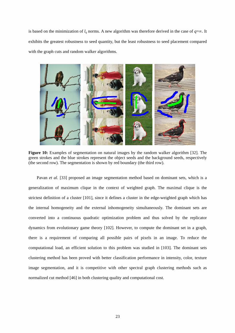
Figure 10: Examples of segmentation on natural images by the random walker algorithm [32]. The green strokes and the blue strokes represent the object seeds and the background seeds, respectively (the second row). The segmentation is shown by red boundary (the third row).

Pavan et al. [33] proposed an image segmentation method based on dominant sets, which is a

generalization of maximum clique in the context of weighted graph. The maximal clique is the

strictest definition of a cluster [101], since it defines a cluster in the edge-weighted graph which has

the internal homogeneity and the external inhomogeneity simultaneously. The dominant sets are

converted into a continuous quadratic optimization problem and thus solved by the replicator

dynamics from evolutionary game theory [102]. However, to compute the dominant set in a graph,

there is a requirement of comparing all possible pairs of pixels in an image. To reduce the

computational load, an efficient solution to this problem was studied in [103]. The dominant sets

clustering method has been proved with better classification performance in intensity, color, texture

image segmentation, and it is competitive with other spectral graph clustering methods such as

normalized cut method [46] in both clustering quality and computational cost.

24

4. Evaluation of Image Segmentation Methods

In previous sections, we have reviewed many graph based methods of image segmentation. It is well-

known that image segmentation is an ill-posed problem, which makes the evaluation of a candidate

algorithm a very challenging work. The most usual way of evaluation is to visually observe different

segmentation results by the user. However, it is time consuming and may result in different outcomes by

users. Quantitative evaluation of segmentation is hence more preferable in practice. In supervised

evaluation, the task is performed by measuring the similarity between the segmentation results and

some ground truth images, which are provided by human observers. This has been widely used by

researchers.

For most segmentation methods, an objective evaluation often requires a measure of

segmentation to have the following characteristics [104]:

Adaptive accommodation of refinement. Since human perceives images in different levels of

details, it is reasonable to compensate for the difference in granularity by allowing refinement

through the image.

Non-degeneracy. The measure will not give abnormally high value of similarity when

confronted unrealistic segments.

No assumption about data generation. The measure should be available for any class of labels

or region sizes.

Comparable scores. The measure gives scores that permit meaningful comparison between

different segmentations.

To quantitatively evaluate the segmentation results, as in [133-134]) we use five well-known

indices: Probabilistic Rand (PR) index [107], Normalized Probabilistic Rand (NPR) index [107],

Variation of Information (VI) [131], Global Consistency Error (GCE) [106] and Boundary

Displacement Error (BDE) [132].

Probabilistic Rand (PR) index. The PR index defines the correctness of segmentations under a

statistical point of view. It is supposed that the segmentation of an image can be described in the form

25

of binary numbers )( kSj

kSi ll =I on each pair of pixels (xi, xj). The distribution of these numbers

follows a Bernoulli distribution and gives a random variable with expected value denoted by pij. The

PR index of two segmentations is then defined as:

( ) 1,{ } ( ) ( )(1 )

2

test test test testS S S Stest K i j ij i j ijPR S S l l p l l p

N⎡ ⎤= = + ≠ −⎣ ⎦⎛ ⎞

⎜ ⎟⎝ ⎠

∑ I I (10)

where N is the number of pixels, {Sk} is the set of ground truth segmentations, pij is the ground truth

probability that the labels of (xi, xj) are the same. In practice, the mean pixel pair relationship in all

ground truth segmentations is used to compute pij. We could see that the penalization of segmentation

for being/not-being in the same region is dependent on the fraction of disagreeing with the ground

truth data. The PR index takes values in the range [0, 1], where a score of zero indicates the labeling

of test image is totally opposite to the ground truth segmentation and 1 indicates that they are the

same on every pixel pair. The PR index accommodates the region refinements appropriately in that it

accepts refinement only in regions that human observers find ambiguous. This property is more

preferable than the refinement-invariant measures for preventing the degenerate cases.

Normalized Probabilistic Rand (NPR) index. From the definition of PR index, however, it is

impossible to know if a given score is good or bad. By introducing an excepted value for a given

segmentation, the NPR is proposed by using a normalization scheme:

index Expectedindex Maximum

index ExpectedIndexindex Normalized−

−= (11)

The maximum index can be set to 1. The expected value of NPR is given as follows:

( ) ( ){ },

' '

,

1,{ } ( ) ( ) 1

21 (1 )(1 )

2

test test test testS S S Stest k i j ij i j ij

i ji j

ij ij ij iji ji j

E PR S S E l l p E l l pN

p p p pN

⎡ ⎤ ⎡ ⎤= = + ≠ −⎡ ⎤⎣ ⎦ ⎣ ⎦ ⎣ ⎦⎛ ⎞⎜ ⎟⎝ ⎠

⎡ ⎤= + − −⎣ ⎦⎛ ⎞⎜ ⎟⎝ ⎠

∑

∑

I I≺

≺

(12)

26

The 'ijp is to be estimated from segmentations of all images:

( )'

1

1 1k k

KS S

ij i jk

p II l lK

Φ Φ Φ

Φ =Φ

= =Φ∑ ∑ (13)

where Φ is the number of different images in the dataset, and KΦ is the number of ground truth

segmentations of image ϕ. NPR index overcomes the flaw of PR, and allows a comparison between

different segmentations of the same image or of different images.

Variation of Information (VI). Meila [131] proposed an information-theoretic distance of clustering.

For segmentations, it can be interpreted as the average conditional entropy of one segmentation given

the other:

)()(),( testKKtestKtest SSHSSHSSVI += (14)

The first term in Eq. (14) measures the amount of information about testS that we loose, while the

second term measures the amount of information about KS that we have to gain, when going from

segmentation testS to ground truth KS . An equivalent expression of Eq. (14) is:

),(2)()(),( KtestKtestKtest SSISHSHSSVI −+= (15)

where H and I are respectively the entropies of and the mutual information between the segmentation

testS and the ground truth KS .

VI is a distance metric since it satisfies the properties of non-negativity, symmetry and triangle

inequality. If two segmentations are identical, the VI value will be zero. The upper bound of VI is

finite and depends on the number of elements in the segments.

Global Consistency Error (GCE). This evaluation criterion is designed for computing the degree of

overlap of regions. Martin et al. [106] proposed the GCE measure to quantify the segmentation

quality in different granularities. This measure allows for refinement, but suffers from degeneracy. Let

),( ipSR be the set of pixels in segmentation S that contains pixel pi, the local refinement error is

defined as:

27

),(

),(\),(),,(

1

2121

i

iii pSR

pSRpSRpSSE = (16)

This error is not symmetric w.r.t. the compared segmentations, and takes the value of zero when S1 is a

refinement of S2 at pixel pi. GCE is then defined as:

⎭⎬⎫

⎩⎨⎧= ∑∑

ii

ii pSSEpSSE

nSSGCE ),,(),,,(min1),( 122121 (17)

Boundary Displacement Error (BDE). BDE is a boundary based metric to evaluate the

segmentation quality. It defines the error of one boundary pixel as the distance between the pixel and

its closest pixel in the other boundary image. Let B1 represent the boundary point in a segmentation,

an arbitrary point x in B1 to a boundary point B2 of the ground truth is defined as the minimum

absolute distance from x to all the points in B2. So a near-zero mean and a small standard deviation

will indicate a good quality of the image segmentation.

From the above introduction of the five indices, one should note that it is not possible to define a

criterion for comparing segmentations that fits every problem optimally. For example, PR and NPR

are based on examining the relationship between pairs of pixels. As a result, segmentation algorithms

which are concerned with pairs (e.g., graph partitioning) can better use PR and NPR for evaluation.

While for clustering algorithms (e.g., mean-shift) focus on the relationship between a point and its

clustering centroid, VI will be a better choice. A good segmentation will achieve large value of PR

and NPR indices while small values of GCE, VI and BDE. Note that these indices are not designed for

evaluating segmentation quality with multiple ground truths. More information on segmentation

quality evaluation with multiple ground truths can be found in [135].

5. Experiments on Automatic Image Segmentation

In this section, three well-known graph theoretic segmentation methods are selected for our

experiments due to their reasonable performance and publicly available implementations: the MST

based method by Felzenszwalb and Huttenlocher [40] (FH method), the normalized cut by Shi et al.

28

[46] (Ncut method), and the ratio cut by Wang et al. [52] (Rcut method). The FH method represents a

different category of graph based segmentation techniques against the Ncut and Rcut methods as we

introduced in Section 3. The evaluation also shows the consistency of segmentation quality produced

by them. We would like to see the stability of the methods and their variance or bias in different

parameter settings. In addition, we make a comparison with the well-known mean-shift method [108],

which does not belong to the graph theoretic category but has been accepted as a robust and efficient

segmentation approach.

All the experiments were performed on the Berkeley dataset [105], where all of the 500 images

are used for our evaluation. These images have 5 to 8 human-marked ground truths on each one of

them. Examples of images are shown in Fig. 11. We can see that there is a high degree of consistency

between different human subjects but a certain variance in the level of details.

Figure 11: Examples of images and their ground truths from the Berkeley image dataset [105].

For each image, we manually choose the optimal set of parameters in each algorithm to achieve

the best evaluation scores. Particularly, in FH method, the smoothing parameter σ was held constantly

to be 0.5, the threshold parameter K was varied through K∈[200, 1500] and the minimum component

size was in the interval of [100,1000]. For Ncut, the number of segments was the only parameter and

it was set from 2 to 20. For Rcut, the linear edge weights were used for both scales and the blending

factor was set as α=0.5. The termination criterion HT was set from 500 to 1200. For mean-shift, the

spatial band width was set from 7 to 25, the color band width was set from 7 to 18 and the minimum

29

region was set from 200 to 2000.

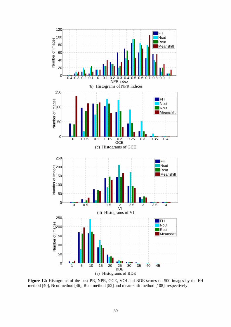
Fig. 12 shows the histograms of five criteria on the 500 natural images. In Fig. 12(a), we see that

the Ncut and Rcut methods have similar best score distributions, which demonstrates their roughly

equal performance on image segmentation. However, since Rcut does not have the shape or boundary-

length bias, it achieves more PR scores over 0.95 than Ncut. In the best performance, nearly all the

algorithms have PR index score above 0.5. And a large portion of segmentations achieves the score

above 0.75. This demonstrates that all the algorithms can produce reasonable results on the test

images. Comparing with the three graph based methods, the mean-shift method can produce more

segmentations whose PR index scores are above 0.85, showing that it performs slightly better than the

three graph based methods. Similar results can be observed in Figs. 12(b)-(e), the general performance

of the four algorithms is acceptable since only a small portion of the segmentation has below-zero

NPR scores. When evaluating the relationship of pixel pairs, Ncut and the Rcut methods have roughly

equal ability to segment the given images. While results by GCE, VOI and BDE show that Rcut

outperforms Ncut for producing more good segmentations, and the mean-shift method outperforms

the three graph based methods in that it produces more scores ranking among the good ones.

0.5 0.55 0.6 0.65 0.7 0.75 0.8 0.85 0.9 0.95 10

20

40

60

80

100

120

PR index

Num

ber o

f Im

ages

FHNcutRcutMeanshift

(a) Histograms of PR indices

30

-0.4 -0.3 -0.2 -0.1 0 0.1 0.2 0.3 0.4 0.5 0.6 0.7 0.8 0.9 10

20

40

60

80

100

120

NPR index

Num

ber o

f Im

ages

FHNcutRcutMeanshift

(b) Histograms of NPR indices

0 0.05 0.1 0.15 0.2 0.25 0.3 0.35 0.40

50

100

150

GCE

Num

ber o

f Im

ages

FHNcutRcutMeanshift

(c) Histograms of GCE

0 0.5 1 1.5 2 2.5 3 3.5 40

50

100

150

200

250

VI

Num

ber o

f Im

ages

FHNcutRcutMeanshift

(d) Histograms of VI

1 5 10 15 20 25 30 35 40 450

50

100

150

200

250

BDE

Num

ber o

f Im

ages

FHNcutRcutMeanshift

(e) Histograms of BDE

Figure 12: Histograms of the best PR, NPR, GCE, VOI and BDE scores on 500 images by the FH method [40], Ncut method [46], Rcut method [52] and mean-shift method [108], respectively.

31

In the second experiment, we test the stability of FH, Ncut and Rcut algorithms with different

parameter settings. Fig. 13 shows the segmentation results on 5 test images. For each of the competing

algorithms, the parameters were set so that they produce roughly the same number of segments for

comparison. The number of segments in the image ranges from 8 to 80. We can see that as the

parameters change, the FH has stronger ability to extract the main structure of objects than Ncut and

Rcut, especially when the number of segments is large. The quantitative measures of segmentation

quality of Fig. 13 are listed in Table 2. The NPR index is used for its ability to compare segmentations

of different images. It is shown that in most cases the Rcut method has better stability of performance

as the parameters changing for the same image. However, the FH method has better average

segmentation quality than Ncut and Rcut on most of the test images.

Table 2: NPR index for segmentation results in Figure 13.

Image #24077

Algorithms Number of regions Mean (NPR)

Variance (NPR) 8 16 26 38 42 68

FH 0.1646 0.7553 0.8409 0.6346 0.8373 0.8252 0.6764 0.0690 Normalized

cut 0.6720 0.7906 0.7942 0.7906 0.7876 0.7667 0.7670 0.0023

Ratio cut -0.113 0.5854 0.7021 0.7183 0.7339 0.68237 0.5516 0.1086

Image #86000

Algorithms Number of regions Mean (NPR)

Variance (NPR) 5 14 21 33 57 88

FH 0.2187 0.5971 0.5764 0.6064 0.5968 0.5922 0.5313 0.0235 Normalized

cut 0.3147 0.4966 0.4657 0.4674 0.4339 0.4171 0.54326 0.0041

Ratio cut 0.5326 0.5451 0.6076 0.6020 0.5874 0.5767 0.5753 0.0009

Image #219090

Algorithms Number of regions Mean (NPR)

Variance (NPR) 8 13 21 37 62 81

FH 0.5505 0.9080 0.9080 0.8729 0.8737 0.7205 0.8056 0.0205 Normalized

cut 0.6448 0.5902 0.5254 0.4563 0.4275 0.4133 0.5096 0.0089

Ratio cut 0.8063 0.7216 0.7418 0.6804 0.7403 0.7304 0.7368 0.0017

Image #296059

Algorithms Number of regions Mean (NPR)

Variance (NPR) 9 14 20 37 48 66

FH 0.4438 0.6181 0.5663 0.5693 0.7030 0.6674 0.5947 0.0083 Normalized

cut 0.4573 0.6189 0.5848 0.5619 0.5487 0.5302 0.5503 0.0030

Ratio cut 0.5931 0.5651 0.5599 0.6101 0.6010 0.5533 0.5804 0.0006

Image #42049

Algorithms Number of regions Mean (NPR)

Variance (NPR) 8 13 28 35 40 63

FH 0.9590 0.9781 0.9715 0.9672 0.9532 0.9161 0.9576 0.0005 Normalized

cut 0.6686 0.5777 0.4547 0.4197 0.4011 0.3709 0.4822 0.0135

Ratio cut 0.9110 0.9610 0.9479 0.9553 0.9408 0.9033 0.9366 0.0006

32

#24077 (a1) FH

(a2) Normalized cut

(a3) Ratio cut

#86000 (b1) FH

(b2) Normalized cut

(b3) Ratio cut

#219090 (c1) FH

(c2) Normalized cut

(c3) Ratio cut

#296059 (d1) FH

(d2) Normalized cut

(d3) Ratio cut

#42049 (e1) FH

33

(e2) Normalized cut

(e3) Ratio cut

Figure 13: Segmentation results under different sets of parameters for FH, Ncut and Rcut algorithms. The number of segments is the same for the three methods on the same image, and changes ascendingly from left to right.

6. Experiments on Interactive Image Segmentation

The goal of interactive image segmentation is to extract semantic objects from an image, and thus it

often turns out to be the form of foreground/background extraction. The comparison of interactive

segmentation methods is not as that objective as the automatic ones. Usually, the performance is

dependent not only on the computational strategies but also the user’s guidance. The user interactions

are often input in terms of brush strokes [1-2, 57, 62, 67, 69] or bounding box [82-83], where the

former is more flexible to achieve arbitrary segmentations. However, the lack of objective criteria for

performing user interaction may lead to the unrepeatability and excessive input provision for the

segmentation results. In general, the effort that a user makes in the interaction can be assessed from

several aspects, for example, the amount of seeds, the cognitive load and the precision requirement for

the user. Some extensive studies [109-110] have been made to evaluate interactive segmentation

methods. In this section, we adopt the similar principle for a consistent and fair evaluation, where the

selected interactive segmentation methods can be compared directly by the same interaction pattern.

The selected interactive segmentation methods in the comparison are graph cut (GC) [57],

iterated graph cut (IGC) [69], lazy snapping (LS) [81] and random walker (RW) [32]2. We consider

two criteria for comparing their performance: the segmentation accuracy and the number of

interactions required for the segmentation. The images we used in the experiments are from the

2 Codes of GC and IGC are provided by the authors. LS is implemented by Mohit Gupta and Krishnan Ramnath

http://www.cs.cmu.edu/~mohitg/segmentation.htm . The code of RW is from http://cns.bu.edu/~lgrady/software.html by Leo Grady.

34

Berkeley Segmentation Dataset, where 96 of the 500 images are selected with the ground truths of

100 objects3. Images are chosen so that each of them has one object that could be unambiguously

extracted by the human beings.

Some qualitative comparisons of the four interactive segmentation methods are shown in Fig. 14.

Given the same amount of user interaction, the performances of these methods are visually different.

We can see that IGC achieves better segmentation results than the other three methods. And most of

the segmentation results are acceptable.

Original Image GC IGC LS RW

Figure 14: Segmentation results of GC [57], IGC [69], LS [81] and RW [32] with the same input seeds. The first column shows the original images with seeds. The second to the fifth columns show the segmentation results obtained by GC, IGC, LS and RW, respectively.

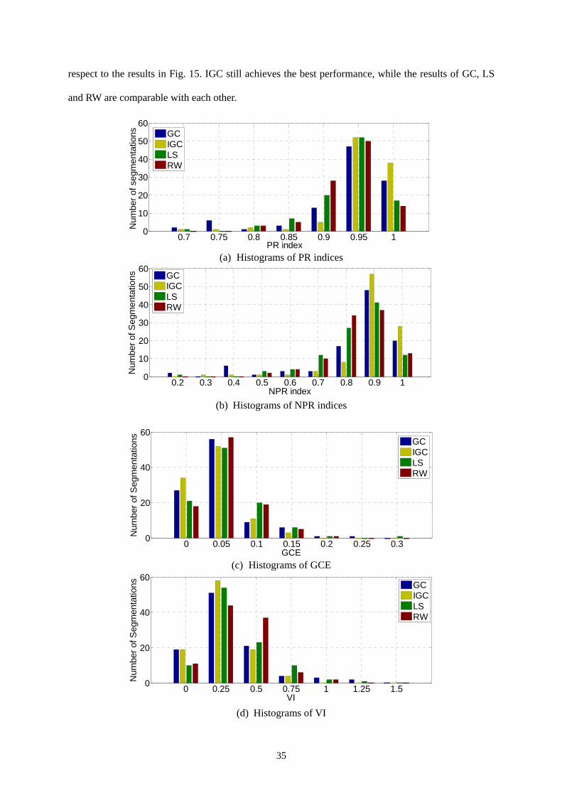
The best performance of each method on the 100 objects in terms of the five criteria are shown in

Fig. 15(a)-(e), respectively. We can see that IGC produces the most segmentations whose evaluation

scores are among the high quality. Both IGC and LS are the extended versions of the GC method.

However, with the iterated optimization of the graph cut energy function, IGC leads to better

segmentation results. Table 3 shows the average segmentation accuracy of the four methods with

3 http://kspace.cdvp.dcu.ie/public/interactive-segmentation/downloads.html

35

respect to the results in Fig. 15. IGC still achieves the best performance, while the results of GC, LS

and RW are comparable with each other.

0.7 0.75 0.8 0.85 0.9 0.95 10

10

20

30

40

50

60

PR index

Num

ber o

f seg

men

tatio

ns

GCIGCLSRW

(a) Histograms of PR indices

0.2 0.3 0.4 0.5 0.6 0.7 0.8 0.9 10

10

20

30

40

50

60

NPR index

Num

ber o

f Seg

men

tatio

ns

GCIGCLSRW

(b) Histograms of NPR indices

0 0.05 0.1 0.15 0.2 0.25 0.30

20

40

60

GCE

Num

ber o

f Seg

men

tatio

ns

GCIGCLSRW

(c) Histograms of GCE

0 0.25 0.5 0.75 1 1.25 1.50

20

40

60

VI

Num

ber o

f Seg

men

tatio

ns

GCIGCLSRW

(d) Histograms of VI

36

1 5 15 20 25 30 35 40 450

20

40

60

BDE

Num

ber o

f Seg

men

tatio

ns

GCIGCLSRW

(e) Histograms of BDE

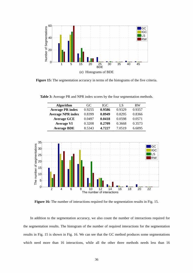
Figure 15: The segmentation accuracy in terms of the histograms of the five criteria.

Table 3: Average PR and NPR index scores by the four segmentation methods.

Algorithm GC IGC LS RW Average PR index 0.9255 0.9586 0.9329 0.9357

Average NPR index 0.8399 0.8949 0.8295 0.8366 Average GCE 0.0497 0.0418 0.0598 0.0571

Average VI 0.3208 0.2709 0.3668 0.3573 Average BDE 8.5343 4.7227 7.0519 6.6095

2 4 6 8 10 12 14 16 18 20 220

5

10

15

20

25

30

35

The number of interactions

The

num

ber o

f seg

men

tatio

ns

GCIGCLSRW

Figure 16: The number of interactions required for the segmentation results in Fig. 15.

In addition to the segmentation accuracy, we also count the number of interactions required for

the segmentation results. The histogram of the number of required interactions for the segmentation

results in Fig. 15 is shown in Fig. 16. We can see that the GC method produces some segmentations

which need more than 16 interactions, while all the other three methods needs less than 16

37

interactions. Table 4 gives the average number of interactions for the segmentations. IGC requires the

least number of interactions among all the methods, while LS requires the most in average. From the

experiments, it is also found that for GC, IGC and LS the seeds should be placed so that they can well

represent the color distribution of the foreground/background regions. For RW, the seeds should be

placed closely to the foreground to get the desirable segmentation.

Table 4: The average number of required interactions by the four segmentation methods.

Algorithm GC IGC LS RW Average number of interactions 6.8 6.71 7.47 6.89

7. Applications in Medical Image Segmentation

In the past years, many real world applications (e.g., medical diagnosis, video surveillance and image

retrieval) have largely benefitted from the graph based segmentation methods. One typical application

is the image based medical diagnosis where specific tissues or organs of interest need to be extracted.

In this section, we review some frequently used methods in medical image segmentation. Although

these methods are designed for specific biomedical imaging applications, most of them can be

classified into one of the five categories introduced in Section 3.

Graph cut based on MRF models (s/t graph cut) [57, 62] incorporates both of the region and

boundary information. It allows for the interactive guidance from the user and no prior model of

objects is required in initialization. More importantly, it can reach the global optima on some

specifically defined graph functions. These features make graph cut based methods produce pleasing

segmentation results for many medical applications. The earliest work was done by Y. Boykov et al.

[111], where the segmentation of one or more objects in both 2D and 3D environments was

implemented. Sophisticated extensions of the s/t graph cut were further proposed to solve the

computation problem on massive grid graph [67], to segment multiple interacting surfaces of a single

n-dimensional object [112-113], to segment multiple objects and surfaces on layered graph [114] and

to extract the multi-surface with some shape prior [115]. Simultaneously segmenting surfaces and

38

objects in a global consistent manner requires considering how the graph is constructed and the

relationship between each surface and object. Formulating the problem on specific graphs provides an

intuitive way to find the mathematically sound solution.

Segmentation of medical objects by extracting contours can be obtained as the shortest path on

the weighted graph. In order to well incorporate the object-related knowledge, the user interaction is

actively pursued and has resulted in better segmentation accuracy. In live-wire methods [116-117], all

possible minimum-cost paths from the seed point to all other points in the image are computed via

Dijkstra’s algorithm [35, 85]. To improve the efficiency, numerous modifications such as live lane [87]

and live wire on the fly [92], which reduce the algorithm’s graph search space, were proposed. The

extensions of live wire to 3D medical images can be found in [93-94, 118-121].

There are also hybrid methods based on the combination of graph theoretic techniques for

medical image segmentation. With the nature of evolution, many active contour models [19,122] find

the path of minimal weighted length within two end points for contour extraction. It has been proven

that under a specific framework, the boundary detection in active contour model is equivalent to the

minimal distance computation in a Riemannian space [98]. Incorporation of shape prior knowledge

has also been extensively studied in the active contour framework, with the statistical shape model

[122-123], the global shape model [124] and the shape of interest [125-126]. The graph search

methods solve the minimal path problems more directly than approximating the solution to PDEs in

the active contour model. With appropriately defined graph structure, the search time and the

computation accuracy are satisfactory to medical applications.

8. Conclusion

In this survey, we systematically discussed representative methods for graph based image

segmentation. These methods are proposed to partition an image into disjoint regions, such that each

region satisfies a certain predefined segmentation criterion. The use of graph as a representation of the

image provides us an effective way to study the problem of image segmentation. The close

relationship between them is not by accident and can be easily understood in two folds. First, the

39

graph is a good mathematical model to describe the discrete characteristics of the real world images.

Second, there are many mature graph theories available to solve the clustering problem, which is

another interpretation of the image segmentation problem. In the past decades, the study of graph

based image segmentation has been making large progress. Particularly, in recent years the emergence

of many new algorithms proves that this category of techniques is still a promising research direction

in the image segmentation community. Further study can refer to versatile graph based algorithms for

a wide range of practical applications. The choice of which method to use is often application specific,

and we argue that the successful ones should utilize appropriate graph models and guarantee good

properties of the segments.

Several open issues still exist in this area. Many graph based methods convert the image

segmentation into an optimization framework, while most of them are NP-hard to solve. Researchers

often try to find alternative solutions to approximate the original problems, and some of them might

result in unpredictable performance in general cases [60]. It is also not easy to find a single

quantitative measure for evaluating the segmentation quality, even with a group of ground truth given

beforehand. To some extent, the evaluation criterion might vary in different applications.

Acknowledgement

We thank the reviewers for their constructive comments in the writing of this survey paper.

References

1. G. Funka-Lea, Y. Boykov, C. Florin, M.-P. Jolly, R. Moreau-Gobard, R. Ramaraj, and D. Rinck. Automatic heart isolation for CT coronary visualization using graph-cut. In IEEE International Symposium on Biomedical Imaging (ISBI), pp.614-617, 2006.

2. L. Grady, Y. Sun and J. Williams. Three Interactive Graph-Based Segmentation Methods Applied to Cardiovascular Imaging. In Mathematical Models in Computer Vision: The Handbook, 453-469. Springer, 2006.

3. Marie-Pierre Jolly, Hui Xue, Leo Grady and Jens Guehring. Combining Registration and Minimum Surfaces for the Segmentation of the Left Ventricle in Cardiac Cine MR Images. Proc. of MICCAI. pp. 910-918, 2009.

4. K.H. Seo, J.H. Shin, W. Kim and J.J. Lee, Real-time object tracking and segmentation using adaptive color snake model, International Journal of Control, Automation, and Systems 4 (2), pp. 236–246, 2006.

40

5. Chun Leung Lam, Shiu Yin Yuen. An unbiased active contour algorithm for object tracking. Pattern Recognition Letters. 19(5-6): 491-498, 1998.

6. S. Yu, R. Gross and J. Shi. Concurrent Object Segmentation and Recognition with Graph Partitioning. Neural Information Processing Systems, NIPS, December 2002.

7. B. Russell, A. Efros, J. Sivic, W. Freeman, A. Zisserman. Using multiple segmentations to discover objects and their extent in image collections. In: CVPR, 2006.

8. P. Favaro and S. Soatto. A variational approach to scene reconstruction and image segmentation from motion blur cues. Proc. IEEE International Conference of Computer Vision and Pattern Recognition. pp. I- 631, 2004.

9. M. Bleyer and M. Gelautz. Graph-based surface reconstruction from stereo pairs using image segmentation. In SPIE, 5665: 288– 299, 2005.

10. M. Wertheimer, Laws of Organization in Perceptual Forms (partial translation). A Sourcebook of Gestalt Psycychology, W.B.Ellis, ed., pp. 71-88, Harcourt, Brace, 1938.

11. R.C. Gonzalez and R.E. Woods. Digital Image Processing. Addison Wesley, Reading, MA, 1992. 12. J. Canny. A Computational Approach to Edge Detection, IEEE Trans. Pattern Analysis and

Machine Intelligence, vol. 8, pp. 679-698, 1986. 13. B. Paul, L. Zhang and X. Wu. Canny edge detection enhancement by scale multiplication. IEEE.

Trans. on Pattern Analysis and Machine Intelligence. 27: 1485-1490, 2005. 14. J. S. Weszka and A. Rosenfeld. Threshold evaluation techniques. IEEE Trans. Syst. Man Cybern.

SMC-8, 627-629, 1978. 15. A. Rosenfeld and P. De la Torre, Histogram concavity analysis as an aid in threshold selection.

IEEE Trans. Syst. Man Cybern. SMC-13, 231-235. 1983 16. J. Weszka and A. Rosenfeld. Histogram modification for threshold selection. IEEE Trans. Syst.

Man Cybern. SMC-9, 38-52, 1979. 17. J.A. Sethian. Level Set Methods and Fast Marching Methods. Cambridge University Press. 1999. 18. S.J. Osher and R.P. Fedkiw. Level Set Methods and Dynamic Implicit Surfaces. Springer Verlag.

2002. 19. M. Kass, A. Witkin and D. Terzopoulos, Snakes: Active contour models. Int. J. of Computer

Vision, 1(4):321–331. 1988. 20. S.J. Osher and J.A. Sethian. Fronts propagation with curvature dependent speed: Algorithms

based on Hamilton–Jacobi formulations. J. of Comp. Phys., 79:12-49. 1988.. 21. D. Cremers, S.J. Osher and S. Soatto, Kernel density estimation and intrinsic alignment for shape

priors in level set segmentation. Int. J. of Computer Vision, 69(3):335-351. 2006. 22. J. Ning, L. Zhang, D. Zhang and C. Wu. Interactive Image Segmentation by Maximal Similarity

based Region Merging. Pattern Recognition, vol. 43, pp. 445-456, Feb, 2010 23. Abraham Duarte, Ángel Sánchez, Felipe Fernández and Antonio S. Montemayor. Improving

image segmentation quality through effective region merging using a hierarchical social metaheuristic. Pattern Recognition Letters. 27(11): 1239-1251, 2006.

24. M. Sezgin and B. Sankur. Survey over image thresholding techniques and quantitative performance evaluation. Journal of Electronic Imaging, 13(1):146-168, 2004.

25. D. L. Pham, C. Xu, J. L. Prince A Survey of Current Methods in Medical Image Segmentation. In Annual Review of Biomedical Engineering, 2: 315-338, 2000.

26. J. A. Noble, D. Boukerroui. Ultrasound image segmentation: a survey. IEEE Transactions on In Medical Imaging. 25(8): 987-1010. 2006.

27. D. Cremers, M. Rousson, R. Deriche. A review of statistical approaches to level set segmentation: Integrating color, texture, motion and shape. International Journal of Computer Vision. 72:195-215, 2007.

28. O. Wirjadi. Survey of 3d image segmentation methods. Technical Report, Fraunhofer ITWM, Kaiserslautern, 2007.

29. N. Senthilkumaran1 and R. Rajesh. Edge Detection Techniques for Image Segmentation-A Survey of Soft Computing Approaches. International Journal of Recent Trends in Engineering, 1(2):250-254, 2009.

30. Z. Wu and R. Leahy. An optimal graph theoretic approach to data clustering: Theory and its application to image segmentation. IEEE. Trans. on Pattern Analysis and Machine Intelligence.15(11):1101-1113, 1993.

41

31. Y. Boykov, O. Veksler and R. Zabih. Fast Approximate Energy Minimization via Graph Cuts. In International Conference on Computer Vision, I: 377-384, 1999.

32. L. Grady. Multilabel random walker segmentation using prior models. In IEEE Conference of Computer Vision and Pattern Recognition. 1: 763-770, 2005.

33. M. Pavan and M. Pelillo. A new graph-theoretic approach to clustering and segmentation. In Proc. IEEE Conf. Computer Vision and Pattern Recognition. 1: 145-152, 2003.

34. Joseph. B. Kruskal. On the Shortest Spanning Subtree of a Graph and the Traveling Salesman Problem. In: Proceedings of the American Mathematical Society, 7(1): 48-50, 1956.

35. E.W. Dijkstra. Some theorems on spanning subtrees of a graph. Indag. Math. 22(2): 196-199, 1960.

36. R.C. Prim. Shortest connection networks and some generalizations, Bell system technical journal. 36(6): 1389-1401, 1957.

37. C.T. Zahn. Graph-theoretic methods for detecting and describing gestalt clusters. IEEE Transactions on Computing. 20: 68-86, 1971.

38. O.J. Morris, M. de J. Lee, and A.G. Constantinides. Graph theory for image analysis: An approach based on the shortest spanning tree. In IEE Proc. F., Communications. Radar & Signal Processing. 133: 146–152, 1986.

39. S.H. Kwok and A.G. Constantinides. A Fast Recursive Shortest Spanning Tree for Image Segmentation and Edge Detection. IEEE Trans. on image processing. 6(2): 328-332, 1997.

40. P.F. Felzenszwalb and D.P. Huttenlocher. Efficient graph based image segmentation. International Journal of Computer Vision, 59(2): 167-181, 2004.

41. D. Hoiem, A. Efros, M. Hebert, Automatic photo pop-up. ACM Transactions on Graphics, 24(3):577-584. 2005.

42. D. Hoiem, A. Efros, M. Hebert, Geometric context from a single image. In International conference on computer vision. pp. 654-661, 2005.

43. Z. Wu and R. Leahy. Tissue classification in MR images using hierarchical segmentation. In Proc. IEEE Int. Conf: Medical Imaging.12(1):81-85, 1990.

44. L. R. Ford, Sr. and E. Fulkerson, Flows in Networks. Princeton NJ: Princeton Univ. Press, 1962. 45. R. E. Gomory and T. C. Hu. Multi-terminal network flows. Journal of the Society for Industrial

and Applied Mathematics, 9: 551-570, 1961. 46. J. Shi and J. Malik. Normalized Cuts and Image Segmentation. IEEE Transactions on Pattern

Analysis and Machine Intelligence. 22(8):888-905, 2000. 47. L¨utkepohl, H. Handbook of Matrices. Chichester: Wiley. 1997. 48. L. Hagen, and A. Kahng, New spectral methods for ratio cut partitioning and clustering. IEEE

Trans. Computer-Aided Design, 11 (9), 1074 -1085. 1992. 49. C. Ding, X. He, H. Zha, , M. Gu and H. Simon. A min-max cut algorithm for graph partitioning

and data clustering. In Proceedings of the first IEEE International Conference on Data Mining (ICDM) pp. 107-114. 2001.

50. I.J. Cox, S.B. Rao, Y. Zhong. Ratio Regions: A Technique for Image Segmentation. In Proceedings of the International Conference on Pattern Recognition, pp. 557-564, 1996.

51. S. Wang and J.M. Siskind. Image Segmentation with Minimum Mean Cut. Proc. Eighth Int’l Conf. Computer Vision, vol. 1, pp. 517-524, 2001.

52. S. Wang and J. M. Siskind. Image Segmentation with Ratio Cut, IEEE Transactions on Pattern Analysis and Machine Intelligence, 25(6):675-690, 2003.

53. S. Geman and D. Geman. Stochastic relaxation, Gibbs distribution and the Bayesian restoration of images. IEEE Transactions on Pattern Analysis and Machine Intelligence 6 (6), 721-741. (1984).

54. S. Geman, and D. McClure. Bayesian image analysis: An application to single photon emission tomography. In Proceedings of the Statistical Computing Section, pp. 12– 18. (1985).

55. S. Geman and C. Graffigne. Markov random field image models and their applications to computer vision. In A. M. Gleason (Ed.), Proceedings of the International Congress of Mathematicians: Berkeley. pp. 1496– 1517, 1987.

56. D. Geman, and B. Gidas. Image analysis and computer vision. National Academy Press. Chapter 2, pp. 9-36, 1991.

42

57. Y. Boykov, Gareth Funka-Lea. Graph Cuts and Efficient N-D Image Segmentation. In International Journal of Computer Vision. 70(2): 109-131, 2006.

58. D. Greig, B. Porteous, and A. Seheult, Exact maximum a posteriori estimation for binary images. Journal of the Royal Statistical Society, Series B, 51(2):271-279. 1989.

59. S. Roy and I. Cox. A maximum-flow formulation of the ncamera stereo correspondence problem. In IEEE Proc. of Int. Conference on Computer Vision, pp. 492-499. 1998.

60. V. Kolmogorov and R. Zabih. What energy functions can be minimized via graph cuts. IEEE Transactions on Pattern Analysis and Machine Intelligence, 26(2):147-159, 2004.

61. A.V. Goldberg, and R.E. Tarjan. A new approach to the maximum-flow problem. Journal of the Association for Computing Machinery, 35(4):921-940. 1988.

62. Y. Boykov and V. Kolmogorov. An experimental comparison of min-cut/max-flow algorithms for energy minimization in vision. IEEE Transactions on Pattern Analysis and Machine Intelligence, 26(9):1124-1137. 2004.

63. D.S. Hochbaum. The pseudoflow algorithm for the maximum flow problem. Manuscript, UC Berkeley, revised 2003, Extended abstract in: The pseudoflow algorithm and the pseudoflow-based simplex for the maximum flow problem. Proceedings of IPCO98, June 1998. Lecture Notes in Computer Science, Bixby, Boyd and Rios-Mercado (Eds.) 1412, Springer, pp. 325-337. 1998.

64. O. Juan and Y. Boykov. Active Graph Cuts. In IEEE Conference of Computer Vision and Pattern Recognition.1: 1023-1029, 2006.

65. P. Strandmark, F. Kahl. Parallel and distributed graph cuts by dual decomposition, In Conf. Computer Vision and Pattern Recognition, pp. 2085-2092. 2010.

66. J. Liu, J. Sun. Parallel Graph-cuts by Adaptive Bottom-up Merging. In Conf. Computer Vision and Pattern Recognition, 2010.

67. D. Andrew and Y. Boykov. A Scalable Graph-Cut Algorithm for N-D Grids. In IEEE Conference on Computer Vision and Pattern Recognition.pp:1-8, 2008.

68. A. Blake, C. Rother, M. Brown, P. Perez and P. Torr, Interactive image segmentation using an adaptive gmmrf model. In European Conference on Computer Vision. pp. 428-441 2004.

69. B. Peng, L. Zhang, D. Zhang and J. Yang, Image Segmentation by Iterated Region Merging with Localized Graph Cuts. Pattern Recognition. 44(10): 2527-2538, 2011.

70. L. Vincent, P. Soille. Watersheds in digital spaces: an efficient algorithm based on immersion simulations. IEEE Transactions on Pattern Analysis and Machine Intelligence, 13, 6, pp.583-598, 1991.

71. Y. Boykov, and V. Kolmogorov. Computing geodesics and minimal surfaces via graph cuts. In International Conference on Computer Vision, vol. I, pp. 26–33. 2003.

72. S. Osher and N. Paragios. Geometric Level Set Methods in Imaging, Vision, and Graphics. Springer Verlag, 2003.

73. X. Liu, O. Veksler and J. Samarabandu. Graph Cut with Ordering Constraints on Labels and its Applications. IEEE International Conference on Computer Vision and Pattern Recognition, pp.1-8, 2008.

74. J. Winn and J. Shotton. The layout consistent random field for recognizing and segmenting partially occluded objects. IEEE International Conference on Computer Vision and Pattern Recognition, pp. I: 37-44, 2006.

75. D. Hoiem, C. Rother, and J. Winn. 3d layout crf for multi-view object class recognition and segmentation. In Computer Vision and Pattern Recognition, pp. 1-8, 2007.

76. Y. Boykov, V. Kolmogorov, D. Cremers and A. Delong. An integral solution to surface evolution PDEs via geo-cuts. In European Conference on Computer Vision, LNCS 3953, 3: 409-422. 2006.

77. D. Freedman, T. Zhang. Interactive graph cut based segmentation with shape priors. In: Computer Vision and Pattern Recognition. I: 75-762, 2005.

78. D. Cremers. Dynamical statistical shape priors for level set based tracking. IEEE Trans. on Pattern Analysis and Machine Intelligence. Vol. 28, pp 1262-1273, 2006.

79. P. Das, O. Veksler, V. Zavadsky, Y. Boykov. Semiautomatic Segmentation with Compact Shape Prior., Canadian Conference on Computer and Robot Vision, pp. 26-38, 2006.

43

80. O. Veksler. Star Shape Prior for Graph-Cut Image Segmentation. European Conference on Computer Vision, pp. 454-467, 2008,

81. Y. Li, J. Sun, C. K Tang and H.Y Shum. Lazy Snapping. ACM Transaction on Graphics. 23(3):303-308, 2004.

82. C. Rother, V. Kolmogorov and A. Blake. Grabcut interactive foreground extraction using iterated graph cuts. In ACM Transactions on Graphics. 23(3):309-314, 2004.

83. V. Lempitsky, P. Kohli, C. Rother, and T. Sharp, Image Segmentation with a bounding box prior, IEEE International Conference on Computer Vision, pp.277-284,2009.

84. J. Liu, J. Sun, and H.Y. Shum. Paint Selection. SIGGRAPH 2009. 85. E. W. Dijkstra, A note on two problems in connexion with graphs, Numer. Math. 1, 269-271,

1959. 86. J. Gross and J. Yellen. Graph theory and its applications. CRC Press; 1 edition. 1998. 87. A.X. Falcão, J.K. Udupa, S. Samarasekara and S. Sharma. User-steered image segmentation

paradigms: Live wire and live lane. In Graphical Models and Image Processing. 60: 233-260, 1998.

88. A.X. Falcão, J.K. Udupa, S. Samarasekera and B.E. Hirsch. User steered image boundary segmentation. In SPIE Proc. Medical Imaging. 2710: 278-288, 1996.

89. A. Martelli. An application of heuristic search methods to edge and contour detection. Commun. ACM, vol. 19, pp. 73-83, 1971.

90. U. Montanari. On the optimal detection of curves in noisy pictures. Commun. ACM, vol. 14, no. 5, pp. 335-345, 1971.

91. D. Pope, D. Parker, D. Gustafson and P. Clayton. Dynamic search algorithms in left ventricular border recognition and analysis of coronary arteries. Comput. Cardiol., vol. 9, pp. 71-75, 1984.

92. A.X. Falcão, J.K. Udupa and F.K. Miyazawa. An ultra-fast user-steered image segmentation paradigm: live wire on the fly. IEEE Transactions on Medical Imaging, vol.19(1):55-62, 2000.

93. A. X. Falcão and J. K. Udupa. Segmentation of 3D objects using livewire. In SPIE Proc. Medical Imaging. vol. 3034, pp. 228-239, 1997.

94. G. Hamarneh, J. Yang, C. McIntosh, M. Langille. 3D live-wire-based semiautomatic segmentation of medical images. In: Proceedings of the SPIE medical imaging: image processing, vol. 5747. p. 1597–603. 2005.

95. E.N. Mortensen and W.A. Barrett. Intelligent scissors for image composition. In Proc. Computer Graphics, pp. 191–198. 1995.

96. X. Bai, G. Sapiro. A geodesic framework for fast interactive image and video segmentation and matting. International Conference on Computer Vision, pp.1-8, 2007.

97. L.D. Cohen and R. Kimmel. Global minimum for active contour models: A minimal path approach. International Journal of Computer Vision. 24(1): 57-78, 1997.

98. V. Caselles, R. Kimmel and G. Sapiro. Geodesic active contours. International Journal of Computer Vision. 22(1): 61-79, 1997.

99. P. Doyle and L. Snell, Random walks and electric networks, ser. Carus mathematical monographs. Washington, D.C.: Mathematical Association of America. no. 22, 1984.

100. S. Kakutani. Markov processes and the Dirichlet problem. Proc. Jap. Acad., vol. 21, pp. 227–233, 1945.

101. J.G. Auguston and J. Minker. An analysis of some graph theoretical clustering techniques. J. ACM, 17(4):571– 588, 1970.

102. J.W. Weibull. Evolutionary Game Theory. MIT Press, Cambridge, MA, 1995. 103. M. Pavan, M. Pelillo, Efficiently Segmenting Images with Dominant Sets. Rivista Lecture Notes

in Computer Science. 3212: 170-24. 2004. 104. R. Unnikrishnan, C. Pantofaru, and M. Hebert. A Measure for Objective Evaluation of Image

Segmentation Algorithms. Proc. CVPR Workshop Empirical Evaluation Methods in Computer Vision, pp.34-34, 2005.

105. D. Martin, C. Fowlkes, D. Tal, and J. Malik. A Database of Human Segmented Natural Images and Its Application to Evaluating Segmentation Algorithms and Measuring Ecological Statistics. Proc. Int’l Conf. Computer Vision, 2:416-423, 2001.

106. D. Martin. An Empirical Approach to Grouping and Segmentation. PhD dissertation, Univ. of California, Berkeley, 2002.

44

107. R. Unnikrishnan and M. Hebert. Measures of Similarity. Proc. IEEE Workshop Computer Vision Applications, 1:394-394, 2005.

108. D. Comanicu, P. Meer. Mean shift: A robust approach toward feature space analysis. IEEE Trans. on Pattern Analysis and Machine Intelligence, 24: 603-619, 2002.

109. K. McGuinness, N.E. O’Connor, A comparative evaluation of interactive segmentation algorithms, Pattern Recognition 43 (2) 434-444, 2010.

110. K. McGuinness, N.E. O’Connor. Toward automated evaluation of interactive segmentation. Computer Vision and Image Understanding, 115 (6):868-884, 2011.

111. Y. Boykov and M.P. Jolly. Interactive organ segmentation using graph cuts, Medical Image Computing and Computer-Assisted Intervention, pp.147-175, 2000.

112. X. Wu and D. Z. Chen. Optimal surface problem with applications. In Proc. 29th Int. Coll. Automata, Lang. Program. 2380: 1029-1042, 2002.

113. K. Li, X. Wu, D.Z. Chen and M. Sonka. Optimal surface segmentation in volumetric images- a graph-theoretic approach. IEEE Trans. Pattern Analysis and Machine Intelligence. 28(1), pp.119-134, 2006.

114. Y. Yin, X. Zhang, R. Williams, X. Wu, D.D. Anderson and M. Sonka. LOGISMOS-layered optimal graph image segmentation of multiple objects and surfaces: Cartilage segmentation in the knee joint. IEEE Transactions on Medical Imaging. 29(12): pp.2023-2037, 2010.

115. Q. Song, X. Wu, Y. Liu, M. Garvin and M. Sonka. Simultaneous searching of globally optimal interacting surfaces with shape priors. In Proceedings of CVPR, pp. 2879-2886, 2010.

116. W. Barrett and E. Mortensen. Interactive live-wire boundary extraction. Medical Image Analysis. 1:331-41,1997.

117. A. Chodorowski, U. Mattsson, M. Langille and G. Hamarneh. Color lesion boundary detection using live wire. SPIE Medical Imaging.15:89-96, 2005

118. A. Falcão and J. Udupa. A 3D generalization of user-steered live-wire segmentation. Medical Image Analysis. 4:389-402, 2000.

119. K. Lu and W. Higgins. Improved 3D live-wire method with application to 3D CT chest image analysis. SPIE Medical Imaging. pp. 189-203, 2006.

120. G. Hamarneh, J. Yang, C. McIntosh and M. Langille. 3D live-wire-based semi-automatic segmentation of medical images. SPIE Medical Imaging.1:597-603, 2005.

121. M. Poon, G. Hamarneh and R. Abugharbieh. Efficient interactive 3D Livewire segmentation of complex objects with arbitrary topology. Computerized Medical Imaging and Graphics. 32(8): 639-650, 2008.

122. T. F. Cootes, C. J. Taylor, D. H. Cooper and J. Graham, Active shape model-Their training and application. Computer Vision Image Understanding, 61(1):38-59, Jan. 1995.

123. M. E. Leventon, W. E. L. Grimson and O. Faugeras. Statistical shape influence in geodesic active contours. In Proc. IEEE Comput. Soc. Conf. CVPR. 1: 316-323, 2000

124. L. H. Staib and J. S. Duncan. Boundary finding with parametrically deformable models. IEEE Trans. Pattern Analysis and Machine Intelligence, 14(11): 1061-1075, 1992.

125. Y. Chen, S. Thiruvenkadam, H. D. Tagare, F. Huang, D. Wilson and E. A. Geiser. On the incorporation of shape priors into geometric active contours. In Proc. IEEE Workshop Variational Level Set Methods Computer Vision. pp. 145-152, 2001.

126. P. Yan and A. A. Kassim. Medical image segmentation using minimal path deformable models with implicit shape priors. IEEE Transactions on Information Technology in Biomedicine.10(4): 677-684, 2006.

127. R. Ardon and L.D. Cohen. Fast Constrained Surface Extraction by Minimal Paths. Int’l J. Computer Vision. 69(1): 127-136, 2006.

128. R. Ardon, L.D. Cohen and A. Yezzi. A New Implicit Method for Surface Segmentation by Minimal Paths: Applications in 3D Medical Images. Proc. Int’l Workshop Energy Minimization Methods in Computer Vision and Pattern Recognition, A. Rangarajan, ed., pp. 520-535, 2005.

129. L. Grady. Minimal Surfaces Extend Shortest Path Segmentation Methods to 3D. IEEE Trans. on Pattern Analysis and Machine Intelligence. 32(2): 321-334, 2010.

130. A. Sinop and L. Grady. A Seeded Image Segmentation Framework Unifying Graph Cuts and Random Walker Which Yields A New Algorithm. In Proc. of Int’l Conf. Computer Vision, pp.1-8, 2007.

45

131. M. Meila. Comparing clusterings: an axiomatic view. In ICML, pp. 577-584, 2005. 132. J. Freixenet, X. Muñoz, D. Raba, J. Martí and X. Cufí. Yet another survey on image

segmentation: Region and boundary information integration. In European Conference on Computer Vision, pp. 408-422, 2002.

133. Z. Li, X. Wu, S. Chang. Segmentation Using Superpixels: A Bipartite Graph Partitioning Approach. In IEEE International Conference on Computer Vision and Pattern Recognition, 2012.

134. T. Kim and K. Lee. Learning full pairwise affinities for spectral segmentation. IEEE International Conference on Computer Vision and Pattern Recognition, pp. 2101-2108, 2010.

135. B. Peng and L. Zhang. Evaluation of Image Segmentation Quality by Adaptive Ground Truth Composition. In European Conference on Computer Vision, Part III, LNCS 7574, pp. 287-300, 2012.