a graph theoretical model for the analysis...
TRANSCRIPT

A GRAPH THEORETICAL MODEL FOR THE ANALYSIS OF THE
GAME OF FOOTBALL AND A DISCUSSION OF
APPLICATIONS THEREOF
by
PATRICK TAYLOR
A DISSERTATION
Submitted in the partial fulfillment of the requirements
for the degree of Doctor of Philosophy
in the Department of Mathematics
in the Graduate School of
The University of Alabama
TUSCALOOSA, ALABAMA
2009

Copyright Patrick Taylor 2009
ALL RIGHTS RESERVED

ii
ABSTRACT
In this dissertation an epidemiological approach is used to develop a graph
theoretical model for the game of football. This model is a preliminary model due to the
limitation of available resources. Even in its preliminary form, it is evident that
significant information is obtained and easily displayed using graphs and adjacency
matrices. A similar approach may be used in other game-like situations where coaches
(manipulators) make decisions about strategy and tactics in order to prevail over
opponents. In our case, the goal is to create a package of tools for the working
professional in the field, i.e., the football coach and his assistants. As a study, this paper
discusses its construction and methods, including procedures used to collect the data,
analysis of the data, conclusions drawn, and commentary on future designs.

iii
LIST OF ABBREVIATIONS AND SYMBOLS
B Line backer
E Defensive end
T Defensive tackle
N Nose guard
C Corner back
F Free safety
SS Strong safety
X Offensive center
O Offensive player other than the center
Offensive ball carrier
Gi,k The (i,k) element of matrix G
Hi,k The (i,k) element of matrix H
Di,k The (i,k) element of the distance matrix D
TGI The total game index of a game
iTGI The total game index of game i
maxTGI The maximum total game index of all the games
minTGI The minimum total game index of all the games
scaledTGI The scaled total game index of a game

iv
V The set of Vertices
E The set of Edges
G = (V, E) A digraph consisting of the vertices from V and edges E
Vi Vertex i
E(Vi, Vj) The edge connecting vertex I to vertex j
Λ The index set
M The adjacency matrix for graph G
d(Vi, Vj) The distance between vertex i and vertex j
R A ring
R[x] The polynomial ring over R
g The Gould Accessibility Index function
l(Vi, Vj) The least weight path from vertex i to vertex j
wd(Vi, Vj) The wandering Distance from Vertex i to vertex j
S Subset of a set
acc(vi) Associated accessibility function of vertex i
Kn Complete weighted digraph
Km,n Complete weighted bipartite digraph
D(Vi) The degree of vertex i
)EV,( t=tG The transpose of G
e(Vi) The eccentricity of vertex Vi
C Covering set
)E(S,C ′= A Circuit
BA ∪ The union of sets A and B
v
BA ∩ The intersection of sets A and B
BA ⊆ A is a subset of B
|S| The Cardinality of set S
AxB The Cartesian product of Sets A and B
Aa ∈ a is an element of A
Aa ∉ a is not an element of A
)E(S,T ′= A tree
),V( E′=Ω The orientation of a graph
f(i, j) The flow from vertex i to vertex j
k(i) The capacity of vertex i
Xi The ith
element of the dominant eigenvector
Xmin The minimum entry of dominant eigenvector
Xmax The maximum entry of dominant eigenvector
Xnormal The Gould Accessibility Index Vector

vi
Definitions
1. Down – The one of four opportunities for an offensive team to gain 10 yards.
They are known as first down, second down, third down, and fourth
down.
2. Distance – The remaining distance that the offensive team must gain for a first
down.
3. Rushing play – An offensive play in which the offensive team chooses to run the
ball instead of passing it.
4. Passing play – An offensive play in which the offensive team attempts to throw
the ball forward in an attempt to gain yards.
5. Hash – A pair of marks that are located 53’4” from either sideline. They are used
to break the field into thirds.
6. Direction – The side of the offense to which the play is run.
7. Left – A play that is run to the left of the left guard.
8. Middle – A play that is run between the right guard and left guard.
9. Right – A play that is run to the right of the right guard.
10. Wide side of the field – The side of the field to which there is a greater distance
from the spot of the ball to the sideline. Any play run in
this direction is said to be ran to the wide side of the field.
11. Short side of the field –The side of the field to which there is a lesser distance
from the spot of the ball to the sideline. Any play run in

vii
this direction is said to be run to the short side of the
field.
12. Neither side of the field – A play that is run to neither the wide side nor short side
of the field. This could be because of two reasons. First,
the play is run up the middle. Second, the ball started in
the middle of the field so there is no wide or short side
since both directions are approximately the same distance
to the sideline.
13. Blown dead – A play that is ended prematurely due to the referee’s whistle.
14. Long – Any down in which the distance to gain is 7 or more yards.
15. Medium - Any down in which the distance to gain is between and including 4 and
6 more yards.
16. Short – Any down in which the distance to gain is 3 yards or less.
17. Snap – The act of passing the ball from the center to the quarterback to start the
play.
18. Pre-snap – Anything that occurs before the play is started.
19. Post-snap – Anything that occurs after the play is started.
20. Blowout Win – A game won by more than 14 points.
21. Blowout Losses – A game lost by more than 14 points.
22. Close Win – A game won by less than 14 points.
23. Close Loss – A game lost by less than 14 points.
24. Chains – The set of two sticks connected by a 10 yard chain that are used to
measure the distance needed for a first down.

viii
25. Adjacency Matrix – The n x n matrix representing a graph G with n vertices in
which aij = 1 if there exists a path from vi to vj and aij = 0
otherwise.
26. Digraph – A graph whose paths are assigned an orientation.
27. Gould Accessibility Index – The normalized eigenvector for the largest
eigenvalue where each vertex is associated with the
corresponding row in the normalized eigenvector.
28. Connected Graph – A digraph is said to be connected if for every pair of vertices
x,y there exists a path from x to y.
29. Weighted Graph – A graph having a weight, or number, associated with each
edge.
30. Weighted Adjacency Matrix – The n x n matrix representing a graph G with n
vertices in which aij = wij if there exists a path
from vi to vj where wij is the weight associated
with the particular edge and aij = 0 otherwise.

ix
ACKNOWLEDGEMENTS
Many people have been a tremendous help to me. Without their assistance, this
dissertation would never have been possible.
First of all, I would like to thank Dr. Joseph Neggers, my advisor, for helping me
through this process. His guidance has been invaluable. He has taught me so much during
my years at the University of Alabama.
Second, I would like to express my gratitude to my committee members: Dr.
Walter Teaff, Dr. Paul Allen, Dr. Wei-Shen Hsia, Dr. Layachi Hadji, and Dr. Zhijian Wu.
Also, I would like to thank the faculty and staff in the Mathematics Department.
Third, I would like to thank all the coaches who assisted me by participating in
the surveys. I am especially grateful to Coach Gene Mitchell, Coach Lonnie Robinson,
Coach Kenny Aycock, and Coach Jeremy Mitchell for teaching me the game of football.
In addition, I would like to thank Coach Jeff Peek for being my test audience and for
helping me convert game films to digital files.
Next, I want to thank my best friend, Coach Josh Sutton. During our many
discussions about this dissertation, he has been my sounding board. I appreciate all his
comments and suggestions.
Finally, I want to thank my family for their love and support. My parents, Andre
and Jeannette Taylor, have always pushed me to be the best person I can be. If not for the
work ethic which they instilled in me, I would not be where I am today. To my brother
Heath and my sister Leigh, thanks for all your help and encouragement.

x
CONTENTS
ABSTRACT ii
LIST OF ABBREVIATIONS AND SYMBOLS iii
DEFINITIONS vi
ACKNOWLEDGEMENTS ix
LIST OF FIGURES xii
CHAPTER 1 1
1.1 GRAPH THEORY REVIEW 1
CHAPTER 2 16
2.1 INTRODUCTION 16
2.2 SCALE 17
2.3 USEFULNESS 17
2.4 THE GAME OF FOOTBALL 18
2.5 SELECTION OF CANDIDATE TEAM 21
2.6 THE CHEROKEE INDIANS 22
CHAPTER 3 26
3.1 QUESTIONNAIRES 26
3.2 RESULTS OF THE QUESTIONNAIRES 28
3.3 CONSIDERATION OF THE FACTORS 29
3.4 RETRIEVAL OF DATA 31

xi
3.5 CONVERSION OF DATA 32
CHAPTER 4 33
4.1 THE ADJACENCY MATRICES 33
4.2 DIGRAPHS OF THE GAMES 34
CHAPTER 5 38
5.1 DISTANCE 38
5.2 DISTANCE ANALYSIS 38
5.3 CLOSE WINS AND LOSSES 40
5.4 TOTAL GAME INDEX 41
5.5 GOULD ACCESSIBILITY INDEX 45
CHAPTER 6 47
6.1 CONCLUSIONS 47
6.2 OTHER APPLICATIONS 48
6.3 FUTURE ENDEAVORS 49
BIBLIOGRAPHY 51
APPENDIX A ADJACENCY MATRICES 53
APPENDIX B DIGRAPHS OF THE GAMES 69
APPENDIX C DISTANCE MATRICES 76
APPENDIX D GOULD ACCESSIBILITY INDEX 88
APPENDIX E INSTITUTIONAL REVIEW BOARD APPROVAL 94

xii
LIST OF FIGURES
Figure 1.1 Example Digraph 2
Figure 1.2 Seven Bridges of Konigsberg Graph 2
Figure 1.3 Multigraph Example 1 3
Figure 1.4 Multidigraph Example 2 3
Figure 1.5 Weighed Euler Graph 3
Figure 1.6 Final Version of Euler Graph 4
Figure 1.7 Adjacency Matrix for Euler Graph 6
Figure 1.8 Adjacency Matrix for Squared Euler Graph 7
Figure 1.9 Squared Euler Graph 7
Figure 1.10 Weighted Digraph Example 11
Figure 2.4.1 Football Field Diagram 20
Figure 2.6.1 Single Wing – Blue 23
Figure 2.6.2 Double Wing – Red 23
Figure 2.6.3 Shotgun 24
Figure 2.6.4 Wishbone 24
Figure 2.6.5 Single Wing X Over – Blue Over 24
Figure 2.6.6 Wing Over – Black 25
Figure 2.6.7 Power I 25
Figure 4.2.1 Offensive Playbook Example Play 37

xiii
Figure 4.2.2 Defensive Alignment Example 37
Figure 5.4.1 Total Distance from Season Average, DT 42
Figure 5.4.2 Scaled Total Distance from Season Average, 43
Figure A.1 Cherokee vs. Colbert Heights Adjacency Matrix 54
Figure A.2 Cherokee vs. Addison Adjacency Matrix 55
Figure A.3 Cherokee vs. Cold Springs Adjacency Matrix 56
Figure A.4 Cherokee vs. Clements Adjacency Matrix 57
Figure A.5 Cherokee vs. Sheffield Adjacency Matrix 58
Figure A.6 Cherokee vs. Tanner Adjacency Matrix 59
Figure A.7 Cherokee vs. Hatton Adjacency Matrix 60
Figure A.8 Cherokee vs. Red Bay Adjacency Matrix 61
Figure A.9 Cherokee vs. Coffee Adjacency Matrix 62
Figure A.10 Cherokee vs. Vincent Adjacency Matrix 63
Figure A.11 Season Total Adjacency Matrix 64
Figure A.12 Blowout Wins Adjacency Matrix 65
Figure A.13 Close Wins Adjacency Matrix 66
Figure A.14 Close Losses Adjacency Matrix 67
Figure A.15 Blowout Losses Adjacency Matrix 68
Figure B.1 Complete Digraph Without Weights 70
Figure B.2 First Down for Season 71
Figure B.3 Second Down for Season 72
Figure B.4 Third Down for Season 73
Figure B.5 Fourth Down for Season 74

xiv
Figure B.6 Sub graph for Season 75
Figure C.1 Distance between Colbert Heights and Season Average 77
Figure C.2 Distance between Addison and Season Average 78
Figure C.3 Distance between Cold Springs and Season Average 79
Figure C.4 Distance between Clements and Season Average 80
Figure C.5 Distance between Sheffield and Season Average 81
Figure C.6 Distance between Tanner and Season Average 82
Figure C.7 Distance between Hatton and Season Average 83
Figure C.8 Distance between Red Bay and Season Average 84
Figure C.9 Distance between Coffee and Season Average 85
Figure C.10 Distance between Vincent and Season Average 86
Figure C.11 Distance between Close Wins and Close Losses 87
Figure D.1 Eigenvalues Part 1 88
Figure D.2 Eigenvalues Part 2 89
Figure D.3 Dominant Eigenvectors Part 1 90
Figure D.4 Dominant Eigenvectors Part 2 91
Figure D.5 Gould Accessibility Indices Part 1 92
Figure D.6 Gould Accessibility Indices Part 2 93
Figure E.1 Institutional Review Board Approval Letter 94

1
CHAPTER 1
1.1 GRAPH THEORY REVIEW
This dissertation is an application of graph theory to the game of football. Thus in
addition to some knowledge of the actual game of football, it will be necessary to discuss
graph theory in its various aspects including pointing out the actual connections
established below between the subject of graph theory and the game of football,
recognizing that in a wider context other and further and possible even deeper bounds
may be established. We begin with a short survey of some definitions and their
consequences in the subject of graph theory.
Graphs as defined in graph theory are usually considered as existing of two sets,
namely, a set V of vertices and a set E of edges. Depending on various specifications on
E, we may have to discuss various types of graphs, these themselves being represented in
a variety of ways for a variety of purposes, as we intend to illustrate below.
The most general type of graphs is what is usually considered to be a weighted
digraph which has a special type as a multidigraph and as a further specialization, a
digraph. If we permit weights which are only non-negative real numbers, then we may
consider the weighted digraph to consist of the set V as indicated above, and the edge set
as being a function E:VxV→[0,∞), the latter denoting the subset of the real numbers used
as the weight set. For those interested in more abstract and general versions of the idea of
what a graph may be, one should note that instead of a function E:VxV→[0,∞), we might
consider E:VxV→ S, where S may be any set with a suitable structure. The set [0,∞) is

2
considered to be equipped with the usual associative and commutative operations + and
*, which are distributive in the usual sense also.
If the set V is finite, then a conventional picture associated with the weighted
digraph often denoted as G = (V, E) is the following:
Figure 1.1 Example Digraph
where the fact that E(Vi, Vj) = 0 as there being no arrow at all.
The famous Euler graph connected with the Seven Bridges of Konigsberg [1]
problem can thus be pictured as shown below with the weights attached to the arrows
(directed edges).
Figure 1.2 Seven Bridges of Konigsberg Graph

3
In the case that the function E:VxV→[0,∞) takes on only integral values, then the
weighted digraph is considered to be a multidigraph, i.e. an arrow such as
Figure 1.3 Multigraph Example 1
is depicted as
Figure 1.4 Multidigraph Example 2
even though in the computational aspects, the effect of one version is completely
equivalent to the effect of the second version of any outcome.
If E(V1, V2) = E(V2, V1) in the edge function of a weighted digraph, then, instead
of a weighted digraph we consider it to be a weighted graph and the arrows become edges
with weights attached. Thus the Euler graph now becomes the figure shown below.
Figure 1.5 Weighed Euler Graph

4
If the weighted edges take on only integral values, then the graph is considered to
be a multigraph and the weighted edge is drawn as a number of edges (a multi-edge)
giving the Euler graph its final form shown below with the seven bridges now very
closely recognizable as the seven edges in the figure.
Figure 1.6 Final Version of Euler Graph
If G = (V, E) is a multigraph, then the degree of a vertex is the number of edges
incident on the vertex and the sequence d(V1) = 5, d(V2) = d(V3) = d(V4) = 3 is the degree
sequence of the Euler multigraph. It is then clear that the sum of the degrees in the degree
sequence is always even for any multigraph. The Havel-Hakini theorem permits one to
determine precisely when a sequence of non-negative integers is the degree sequence of
some multigraph which is usually not unique via an algorithmic method of descent which
permits one to replace a given sequence by a simpler one until one reaches a point where
the decision is obvious. Also, whether the seven bridges problem has a solution can be
decided on entirely graph theoretical principles explained below.
A final step in the organization of this terminology is to consider the case where
E:VxV → 0,1. Then, the weight on the digraph is an integer (a multigraph) and the
“graph” is then considered to be a digraph. If E(Vi, Vj) = E(Vj, Vi) as well, the structure is

5
considered to be a graph. If in addition it is the case that E(Vi, Vi) = 0, then the structure
is considered to be a simple graph. From the illustration above it follows that the Euler
graph is a multigraph where E(Vi, Vi) = 0 for i = 1,2,3, and 4, but it is not a simple graph.
We note that if E:VxV → [0,1] instead of 0,1, then the weighted digraph can be
also considered as a fuzzy subset of the set VxV. Where the value E(Vi, Vj) is considered
to be the “degree to which an arrow Vi → Vj may be present.” Although it is not true that
this represents a probability distribution on VxV unless the “sum” of the E(Vi, Vj) = 1 in
some way, it is also the case that useful modeling of probability flows can be handled by
using weighted digraphs of this type.
Suppose now that G = (V, E) with E:VxV → [0,∞) as given. Then, if
Λ∈= iiVV )( is labeled by the linearly ordered set, we may consider sums
),(),(,),(),(),( 2
jijVVEjiEkiEkjEjiE ==∑ Λ∈
. If Λ is finite then E2:
VxV→ [0,
∞) is always defined. If Λ is not finite, then restrictions is on E may yet guarantee that the
series ∑ Λ∈→
jkiEkjEjiE ),(),(),(
2 in some “reasonable” way. For example, If E has
the finite choice (finite exit) property, then E(i, j) = 0 for all but a finite number of Λ∈j ,
and E2(i, k) is defined. Thus, G
2(V, E
2) is also a weighted digraph, the weight E
2(i, k)
measuring the sum total of the weights of paths (of length 2) from Vi to Vk. If Λ is finite
or if E has the finite choice property then it is certainly the case that one may define a
sequence of mappings En+1
:VxV→ [0, ∞) via the formula
∑ Λ∈
+=j
nn kiEkjEjiE ),(),(),( 1, which in turn yields weighted digraphs
Gn+1
= (V, En+1
). If by ),0[:0 ∞→VxVE we mean that

6
0,0,),(0 =≠== iiijijji jiifVVE δδδ , then one establishes without problem
that nmnm EEE +=* , where m
E , n
E , and nm
E+
are defined according to the principles
established above. The function ),0[:)...( 2 ∞→+++ VxVEEEn
is also defined
in this case and represents a further weighted digraph of interest in many situations,
especially when the case n is very large (approaches ∞) is considered.
In the case that Λ is finite, the function E:VxV → [0,∞) may be represented as a
matrix, the adjacency matrix M(G) = M, where ),( jiEM ij = . Thus, it is easily seen that
),(),()*( kjEjiEMMMM jkijik ∑∑ ∗=∗= , that is the matrix
MMM ∗=2 represents the weighted digraph ),( 22 EVG . The condition that the
function E has the finite choice property then becomes the condition that the adjacency
matrix satisfies the row-finiteness condition.
In the case that ),( EVG is a multidigraph then ijM counts the number of arrows
from Vi to Vj. Similarly ijM )( 2counts the number of paths of length 2 from Vi to Vj.
The matrix ij
nMM )...( ++ then counts the number of paths of length at most n from
Vi to Vj.
The following matrix is the adjacency matrix of the Euler multigraph as pictured
above with M =
Figure 1.7 Adjacency Matrix for Euler Graph
V1 V2 V3 V4
V1 0 1 2 2
V2 1 0 1 1
V3 2 1 0 0
V4 2 1 0 0

7
and with M2 =
Figure 1.8 Adjacency Matrix for Squared Euler Graph
denoting the path length 2 matrix whose multigraph ),( 22 EVG can now be pictured as
show below.
Figure 1.9 Squared Euler Graph
If 0)...( >++ij
nMM for all Λ∈ji, , then pictorially there is a directed path
from Vi to Vj for any pair of vertices Vi and Vj (including i = j). We shall consider a
weighted digraph to be strongly connected if this is the case. If we let d(Vi, Vj) = k if k is
the smallest integer such that 0)( >ij
kM for i ≠ j, while we set d(Vi, Vi) = 0, then
k )V ,d(V ji = and l )V ,d(V tj = implies lk += )V ,d(V ti , that is
V1 V2 V3 V4
V1 9 4 1 1
V2 4 1 2 2
V3 1 2 5 5
V4 1 2 5 5

8
),(),(),( tjjiti VVdVVdVVd +≤ . Indeed, if 0),()...,(),( 1211 >− jaEaaEaiEk
and if
0),()...,(),( 1211 >− tbEbbEbjEl
, then also
0),()...,(),(),()...,(),( 12111211 >−− tbEbbEbjEjaEaaEaiElk
, that is the triangle inequality
holds for d. The condition )V,V(d )V ,d(V ji ij= will then hold if jiij MM = ,
that is E(i, j) = E(j, i), which is the case precisely when ),V( EG = is a weighted graph
so that the function d:VxV → [0, ∞) is a metric and incidentally d) V,(* =G becomes a
weighted digraph whose adjacency matrix *
M has )V ,d(V)( ji
* =ijM , that is, it is
symmetric with 0’s on the main diagonal.
Given a weighted digraph ),V( EG = , let [ )∞→ ,0VxV:tE be the function
),(),( ijEjiE t = and )EV,( t=tG the transpose of ),V( EG = . The if ( )
2
t
s
EEE
+= ,
it is certainly the case that )EV,( s=sG is a weighted digraph and because of the
symmetry, ),(),( ijEjiE s= , it is a weighted graph. If )EV,( s=sG is strongly
connected, then ),V( EG = is considered to be a connected weighted digraph.
The fact that the Euler multigraph is connected can be noted from the figure of
from the fact that 0)( 2 >ijM for all vertices Vi, Vj. Given the fact that
)EV,( s=sG is connected, the eccentricity, e(Vi), of a vertex Vi is )V,d(Vmax jij ,
where Vj ≠ Vi. The diameter of a ),V( EG = is )e(Vmax ii , while the radius of
),V( EG = is )e(Vmin ii , and the diameter is at most twice the radius by the triangle
inequality for the distance function.

9
In terms of modeling algebraic structures, if M is the adjacency matrix of a
weighted digraph ),V( EG = , then over a sub-ring of the complex numbers say R, M
generates a R-module by substitution of M into polynomials p(x) in R[x], the polynomial
ring (algebra) over R. The properties of R[M] then reflect properties of ),V( EG = and in
turn properties of ),V( EG = then determine properties of R[M]. Since by the Cayley-
Hamilton theorem M satisfies its characteristic equation if follows that R[M] is certainly
finitely generated with the powers of M, say,
=∑−
=
1
0
2,...,,
k
i
i
i
kMMMM λ providing a
generating set for R[M].
Given the adjacency matrix, M, of ),V( EG = the linear algebra associated with
M and through M of ),V( EG = has long been a subject of interest as should be clear
from what has already been said above. In particular, the interpretation of the meaning of
eigenvalues of M, that is, the spectrum of M (and of ),V( EG = ) has been of interest . If
),V( EG = is symmetric with E(i, i) = 0, then it follows that M has real eigenvalues. The
sum of these eigenvalues being 0, it also follows that the largest eigenvalue being
positive in the case that M is not the zero matrix corresponding to the set with E(i, j) = 0
indicating the absence of all weighted arrows, the associated (non-zero) eigenvector on
normalization presents a function RV: →g , the Gould accessibility index, whose
values represent an overall property of the paths leading to the given vertices representing
a notion of accessibility. There are other ways to model the concept of accessibility, but
this particular one is a common one used in the area. Given a weighted digraph
),V( EG = , the line graph LG has as vertices the set VxV and an edge function
[ )∞→× 0,VxV)()VxV(:E where 0)xV(V)xV(V:E lkji =× if j ≠ k and

10
l)E(j,j)E(i,)V,(V,)V,(V:E ljji = . Thus if 0)V,(V,)V,(V:E ljji > , then
0l)E(j,j)E(i, > , whence also 0j)E(i, > and 0l)E(j, > , that is , the arrows are incident
on one another. In the case ),V( EG = is a simple graph, then 1,0j)E(i, ∈ and
0k)j)E(j,E(i, > implies 1k)j)E(j,E(i, = as well, while 0j)j)E(j,E(i,l)i)E(i,E(i, == ,
so the vertices are not incident on edges. Eliminating pairs (Vi, Vi) from the discussion, it
is easy to see that for simple graphs ),V( EG = the line graph LG is also a simple graph.
Its eigenvalues are then real and greater than or equal to -2 for example.
Given a weighted digraph ),V( EG = there are various algorithms to determine
the least-weight path from a vertex Vi to a vertex Vj. If
)V,(...,),,(),,V( j1211i −kaEaaEaE all have positive value, then k)V ,d(V ji ≤ since the
product 0)V,()...,(),V( j1211i >−kaEaaEaE . Thus, one may consider
0)V,(...),V( j11i >++ −kaEaE the weight of the particular path from Vi to Vj. Thus, if the
weights of these paths are minimized to obtain the least-weight path, say l(Vi, Vj) > 0 is
the weight of such a path, then again l(Vi, Vj) + l(Vj, Vk) > l(Vi, Vk) and the triangle
inequality holds. If we set l(Vi, Vi) = 0, and if l(Vi, Vj) = l(Vj, Vi) for all I and j, then
[ )∞→ 0,VxV:l is again a metric which corresponds to the metric [ )∞→ 0,VxV:d if
0i) E(i,,0,1j) E(i, =∈ for all Λ∈j i, . Thus for simple graphs this is indeed the case.
An algorithm capable of doing so is the well known Dykstra’s Algorithm [2]. Based on
this parameter, one may then define and eccentricity function [ )∞→ 0,V:e and from
that derive a diameter and a radius with the usual property.
A last distance-like parameter is the wandering distance function
[ )∞→ ,0VxV:wd , where if )jE(i,...,),jE(i, l1 are all positive and 0h)E(i, = otherwise,

11
then )]jE(i,...,),j)/[E(i,jE(i,)j(i,E l1tt =~
represents a “probability” that a transition
from Vi to tj
V is to be made. Using these transition probabilities one can compute the
expected value of the random variable which measures the expected number of steps
required to move from a vertex Vi to a vertex Vj as wd(Vi, Vj). As a simple example, if
the weighted digraph has a diagram:
Figure 1.10 Weighted Digraph Example
then E(1, 1) = E(1, 2) = 1, 2
1(1,2)E
~(1,1)E
~== . Now the probability-generating function
g for this digraph has 2g(V1, V2) = xg(V1, V2) + xg(V2, V2), where g(V2, V2) = 1. Thus
)2( )V ,g(V 21 x
x−
= and )V ,wd(Vx
1)x (at )V ,Vg 21
x
21 ==−
==′
=
2)2(
2(
1
2.
If we consider the associated accessibility function, acc:V→[0, ∞), as
∑ ≠=
ij iji )V,wd(V)V(acc , then 2 )V ,wd(V)V(acc 212 == in the above case.
The game which is modeled is that of flipping a coin, the game ending when tails (T)
turns up. The smaller the acc(Vi), the more accessible the vertex.
A subset S of V in ),V( EG = is independent of E(i, j) = 0 for S Vj Vi, ∈ . The
independence number of a graph is the largest cardinal of a maximal independent subset,
where a maximal independent subset S has the property that if S∉jV , then E(i, j) > 0

12
for S∈iV . If E(i, j) > 0, then Vi covers Vj. A subset C of V is a covering set if C∉jV
implies E(i, j) > 0 for CVi ∈ . The covering number of ),V( EG = is the smallest
cardinal number of a minimal covering set. There are many interesting relations
connecting these two parameters and determination of these numbers is computationally
complex for general graphs. The coloring number is the cardinal number of a minimal
coloring set (also the chromatic number), where such a set has the property that if
0j) E(i, > then they may be colored with distinct colors form the set. The Heawood Four
Color Conjecture [3], (now a theorem) states that planar graphs have chromatic number at
most 4. Planar graphs are simple graphs which can be drawn in a plane without having
edges crossing. A simple graph is planar if and only if it does not contain a
(homeomorph) of K5 or K3,3 by Kuratowski’s Theorem [4]. A weighted digraph version
of K5 has E(i, j) > 0 for i ≠ j, VV,V,V,V,VV 54321i =∈ , while K3,3 has E(i, j) > 0 for i
≠ j, 321i V,V,VV ∈ and 654j V,V,VV ∈ , VV,V,V,V,V,V 654321 = . Kn for n > 3 is
a complete weighted digraph, while Km,n for m + n > 3 is a complete bipartite weighted
digraph.
Given a weighed digraph, ),V( EG = , a circuit (or cycle) is a subgraph
)E(S,C ′= , where VS ⊆ and E SxS) (E ∩⊆′ such that ∞<≤ S3 and such that for
some ordering of kV,...,VS 1= where kS = , 0k)E(k,1)1,-3)...E(kE(1,2)E(2, > , and
no proper subset of E′ has this property. A weighted digraph, ),V( EG = , is a tree if it
contains no circuits. A spanning tree of ),V( EG = is a subgraph )E(S,T ′= of
),V( EG = such that S = V and such that T is a tree. If Kn is a complete simple graph,

13
then it has nn-2
spanning trees by a result of Cayley. For a general simple graph
),V( EG = , its spanning trees may be counted using a formula developed by Poincaré.
Given a weighted digraph, ),V( EG = , an orientation on ),V( EG = is a
weighted digraph ),V( E′=Ω , where j)E(i,j)(i,E ≠′ implies 0j)(i,E =′ , and where
0i)(j,Ej)(i,E =′′ , and where 0i)E(j,j)E(i, >+ implies 0i)(j,Ej)(i,E >′+′ . An
orientated weighted digraph ),V( EG = has an orientation Ω=G . A flow on a
weighted digraph is a function [ )∞→ 0,E:f such that f(i, j) < E(i, j). A cut is a partition
21 V V V ∪= , 21 V V ∩ = . If ),V( EG = has an orientation ),V( E′=Ω and if f is a
flow, then if 0j)(i,E >′ (that is 0j)(i,E =′ ) the net flow with respect to orientation
is i)f(j,-j)f(i, . The capacity of the vertex Vi is 0k(i) with k(i) i)E(k, - j)E(i, == ∑∑∑ .
The capacity of a subset S is the sum ∑ ∈SVi
ik )( . The capacity of VxV )V ,(V ji ∈ is
E(i, j) and the capacity of a subset S of VxV is ∑ ∈SVV ji
jiE),(
),( .If f is a flow and
21 V V ∩ = V is a cut, then the cut determines a subset ( ) 2j1iji VV,VVV , VS ∈∈=
with ∑ ∈SVV ji
jiE),(
),( the capacity of the cut. The capacity of ),V( EG = is the
minimal capacity of a cutset. The flow with respect to any orientation on G is
∑ ∑ji, ij,
i)f(j,-j)f(i, and is at most the capacity of any cutset and thus at most the minimal
capacity of a cutset. This minimum can be reached on finite graphs. Applications of the
theory of flows are manifold in the real world.
Given a finite weighted digraph ),V( EG = , we will consider an ordering of the
set of “edges” ( (Vi, Vj) with E(i, j) > 0). With respect to an orientation ),V( E′=Ω of

14
),V( EG = , we construct an incidence matrix whose rows are labeled by the vertices,
m1 V , ,V … of V is mV = and whose columns are labeled by the “edges” of n1 e , ,e … ,
where )V ,(V e jit = and 0j)(i,E =′ . In that case, if M is the m x n incidence matrix, then
j)(i,EM it′= and j)(i,EM jt
′−= , 0t)(s,E =′ otherwise. Since the column sums are all
equal to 0, the row vectors are linearly dependent and if the weighted digraph ),V( EG =
is connected, its rank is (m-1) by a simple argument. Note that ( ) ∑=k
t
kjikij
t MM MM
and thus ( ) SSj
jk
==′== ∑∑∑ ∈1j)(i,EM MM
22
ikii
t, where 0j)(i,E | jS ≠′= , is
the degree of the vertex i. In that case too, ( ) 2
ijijiiij
t EEE MM −=−= ∑∑kk
, so that if
0,1j)E(i, ∈ , then A- MMt
= , where A is the adjacency matrix of the digraph
),V( EG = .
Using such incidence matrices one may decompose the edge space into the
orthogonal sum of the circuit space and cutest space and use this decomposition further in
applications such as deriving Kirchoff’s Equations [5] in circuit analysis and solving
other problems.
In conclusion, the above short survey of definitions, examples, and results ahs left
unmentioned a great many more possible points which might be discussed profitably. I
have meant to demonstrate that in modeling real world questions these graph theoretical
ideas have proven themselves to be most useful indeed. For example, if ),V( EG =
represents a map of a town, with E(i, j) denoting the length of a street from intersection
Vi to intersection Vj, then a question where one should put a fire station, or on which
intersections should put cameras so that all streets can be surveyed, are questions of the

15
type which may be addressed in the is setting in useful ways, that is, with a hope of one’s
being able to solve the problem posed in a reasonable fashion, that is, reasonable both
from a logical and from a cost conscious viewpoint. Being aware of the potential of graph
theory in such a great variety of settings, it seemed therefore natural to me that I might try
to make use of some graph theoretical ideas in the analysis of decision making processes
employed by coaches of football teams and their staffs. Doing so required me to become
involved with certain practices common to the field of epidemiology as well. What this
required in overcoming certain difficulties in order to arrive at sensible data for the actual
analysis will be discussed in the following along with the actual results obtained there.

16
CHAPTER 2
2.1 INTRODUCTION
The purpose of this dissertation is to find a new way to examine the game of
football. Coaches spend hours breaking down game tapes of the opposition to try to find
any advantage that they can exploit. Every coach uses a different method to break down
the film. Some coaches simply look at the different formations that the offense uses so
that plans can be made how to line up his defense for each formation. Other coaches
record which plays are run in certain situations, such as down and distance, so that they
can try to find a tendency in the offense. The coaches usually meet on the Sunday before
the game on Friday to break down the film and discuss game plans for the week. Then
they will communicate the game plan with the players starting with the practice on
Monday.
I have developed a new method to break down the game film. I have recorded
several factors, which will be discussed later, from the game film, extracted observational
data, and transformed the data into a useful mathematical model. I have then applied
graph theory techniques such as adjacency matrices [6], digraphs [7], and weighted
graphs to create a mathematical model of each game. Although an unusual approach, I
believe that we can gain valuable information from it.
I am limiting the study to the offensive play calls. I chose not to include the
defensive play calls because so much of what the defense does depends on what the
offense does. For example, if a team uses an offensive formation with five wide
17
receivers, a defense is not going to counter with a formation with four linemen and four
linebackers. Likewise, if a team uses an offensive formation with two tight ends and three
running backs, the defense is not going to counter with a formation with five or six
defensive backs. In essence, the defense depends on the offense, or in mathematical
terms, the defense is a function of the offense.
This paper uses many terms that may be unfamiliar to the reader. Since this is a
paper not only on mathematics, but also football, it was necessary to include a definitions
section in the preliminary sections of the paper. These definitions include terms from the
world of football, and graph theory terms. It is necessary to understand these definitions
to gain the full understanding of this paper. These definitions can be found starting on
page xii. Chapter 1 also reviews several graph theory topics that are also useful to the
reader.
2.2 SCALE
This paper is designed to be a small scale feasibility study. The resources necessary for a
full scale, in-depth study are just not available at this time, but hopefully the results found
here will help lead to a full scale study in the future. This study is limited not only by the
amount and quality of the game film, but also by the man-power available to completely
break down the game films, record the data, and sort the data into a usable form. Another
limiting factor is the forced omission of factors that do contribute to play calls, such as
time remaining.
2.3 USEFULLNESS
The first use of this study is to provide high school coaches with a tool to help
prepare their teams for their games. This model can be used to scout the opposition as

18
well as self scouting to make sure that the coaches are not becoming predictable in their
play calls. With further refinement, this model could also have applications as a tool for
football analysts on television. Another possible application is in the video game world.
Every year two of the most anticipated video games released are football games produced
by EA Sports. The two games are NCAA Football and Madden NFL Football. Madden
NFL Football grossed over 100 million dollars in the opening weekend. [8] The model
could lead to a more realistic computer opponent in the game. It would be relatively easy
to analyze a number of NFL or college coaches, and use their actual play calls in their
games to help determine the play calls in the video game.
2.4 THE GAME OF FOOTBALL
This is a brief overview of the game of football. It is only designed to provide the
reader the basic overview of the game. If the readier is interested in more detailed
information, including strategies of the game, there are several books available that
would be beneficial to the reader.
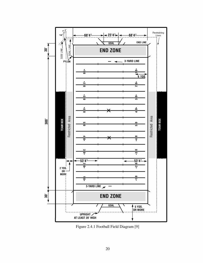
The game of football is played by two teams, each with 11 players on the field at
the same time. The playing field is 300 feet long by 160 feet wide with two end zones
that are 30 feet long by 160 feet wide. A diagram of the field can be seen in figure 2.4.1.
The game consists of 4 quarters that are each 12 minutes long in high school football.
The object of the game is to score more points than the opponent. A team can
score a touchdown, worth 6 points, by advancing the football past their opponent’s goal
line. After scoring a touchdown, the offensive team has the choice to try to kick the
football through the uprights for 1 point or try to advance the football past the goal line
from the three yard line for 2 points. The offensive team can also score by kicking a field

19
goal, worth 3 points. The defensive team can also score by tackling the opposing ball
carrier in the offensive team’s end zone, worth 2 points.
When the offensive team gains possession of the ball, it has 4 downs to gain 10
yards. If the offensive team does not gain 10 yards after these 4 downs, it must turn the
ball over to the defensive team. At this time, the defensive team will go on offense and
the offensive team will switch to defense. If at any time during the 4 downs, the offensive
team gains 10 yards, it will receive a new set of 4 downs to gain 10 more yards. This
process will repeat until either the defensive team stops the offensive team, the defensive
teams creates a turnover, the offensive team scores a touchdown, or the offensive team
attempts a field goal.
20
Figure 2.4.1 Football Field Diagram [9]

21
2.5 SELECTION OF CANDIDATE TEAM
For this dissertation, I decided to focus on one team. I chose the 2000 Cherokee
Indians from Cherokee High School in Cherokee, Alabama. I chose this team for several
reasons. The first reason I chose this team was the availability of game films. Coaches
closely guard their game film. They do not like to take the chance that a copy of a game
film could find its way into an opponent’s possession. It should be noted that the standard
procedure during the season is for each coach to swap the game film from the previous
two games, assuming that two have been played, with the coach of the team that they are
playing that week. This is a gentlemen’s agreement amongst the coaches. The game film
for the 2000 Cherokee Indians was the most easily obtained.
The second reason I chose this team was the simplicity of their offense. Their
offense consisted of approximately 50 plays. The size of the playbook makes it ideal for
study because it is large enough to have a nice balance of running and passing plays, but
is small enough to easily manage analysis. The offense used by the 2000 Cherokee
Indians will be discussed later.
The third reason that I chose this team was my familiarity with the 2000 Cherokee
Indians. As a senior starter on the team that year, I have detailed knowledge of the
playbook, the coaching staff, and the players on the team. This makes it easier to break
down the game films and obtain the most accurate data possible. I can easily recognize
formations and plays. I also know the strengths and weaknesses of the team.
The fourth and final reason that I chose this team was because they had a
balanced season. The Indians finished the year with a record of four wins and six losses,
including a first round loss in the state playoffs. Two of the wins would be classified as

22
blowouts since they won by fourteen points or more. These were against Clements and
Tanner. The other two wins would be classified as close wins since they were by less
than fourteen points. These were against Colbert Heights and Cold Springs. Three of the
losses would be classified as close losses since they were by less than fourteen points.
These were against Addison, Sheffield, and Red Bay. The other three losses would be
classified as blowouts since they were by fourteen points or more. These were against
Hatton, Coffee, and Vincent. This should be ideal for study since we will get a broad
spectrum of the team’s successes and its struggles.
2.6 THE CHEROKEE INDIANS
The 2000 Cherokee Indians were from a 2A school with approximately two
hundred twenty students from grades nine through twelve. The football team consisted of
33 players from grades seven through twelve. The primary offense of the 2000 Cherokee
Indians was the wing-T offense with multiple formations. The team also used a shotgun
formation to try to spread out the defense, a wishbone formation for short yardage and
goal line situations, and a power I formation. The formations can be seen in figures 2.6.1
through 2.6.7. However, the majority of the offensive formations used were wing-T
formations. The wing-T is a misdirection offense which is weighted more to running the
ball than passing the ball. It usually consists of one wide receiver, one tight end, and three
running backs. It usually consists of one wing back, a fullback, and a halfback. An
alternative lineup that consists of two wing backs was also used to try to balance out the
defensive line. The wing-T was a common offense used in high schools in 2000, which
makes it an ideal offense to study. It would be easy to extend the methods used on this
team to other teams using the same offense. The offensive players are designated with
23
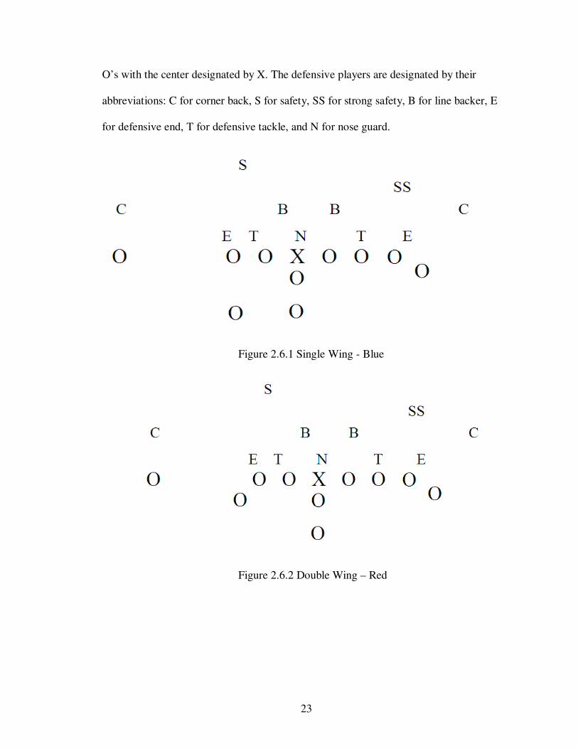
O’s with the center designated by X. The defensive players are designated by their
abbreviations: C for corner back, S for safety, SS for strong safety, B for line backer, E
for defensive end, T for defensive tackle, and N for nose guard.
Figure 2.6.1 Single Wing - Blue
Figure 2.6.2 Double Wing – Red

24
Figure 2.6.3 Shotgun
Figure 2.6.4 Wishbone
Figure 2.6.5 Single Wing X Over – Blue Over

25
Figure 2.6.6 Wing Over – Black
Figure 2.6.7 Power I

26
CHAPTER 3
3.1 QUESTIONNAIRES
The first step in the designing of the model was to create a list of factors that
affect offensive play calling to consider. To aid in the selection of factors to include, I
interviewed a sample of 19 high school coaches from various schools across the state of
Alabama. The sample included coaches at small, medium, and large high schools. At
each of these schools, I chose coaches to interview with a variety of backgrounds. I
interviewed new coaches fresh into the world of coaching, seasoned veterans, and a few
retired coaches. This also led to a variety of the levels of coaches interviewed. I
interviewed varsity head coaches, varsity assistants, junior varsity head coaches, junior
varsity assistants, junior high school head coaches, and junior high school assistants. I
feel that this sample creates a well balanced picture of what goes through a coach’s mind
when he calls a play.
I conducted the interviews by questionnaire. The questionnaire was designed to be
free response to encourage the coaches to elaborate on their responses instead of just
ranking predetermined choices that I made. I feel this is important because it allows the
coach to be free of any bias or influence that I may have subconsciously written into the
question. The questionnaire consisted of ten questions. The questions are listed below.
The Institutional Review Board approval letter can be found in appendix E.
1. How many years have you coached and at which schools?

27
2. How many years have you spent as the offensive coordinator/offensive play
caller and at which schools?
3. What factors do you consider when you decide to make a play call and discuss the
importance of each. If possible, please try to rank the importance of each
factor.
4. What is your offensive philosophy?
5. Do you try to call plays to your strengths or your opponents’ weaknesses?
6. 4th and goal from the 3 yard line with 3 seconds remaining, down by 5 what play
do you call? Why?
7. Do you prefer to run the ball more or pass the ball? Why? (Assuming that your
team is equally proficient at each.)
8. How do you use statistics to break down opposing game tape? Do you chart %
pass/run based on down and distance? Based on formations? Do you chart
what % of the time they go to the wide/short side of the field? To the
left/right/middle?
9. How do you use those statistics during the game?
10. Please give any comments that you would like to add that you think would be
valuable to this project.
The information gained in the survey was combined with my eight years of
experience coaching football at the high school level, as well as the limitations of the
process, to select the factors used to create the adjacency matrices. This will be discussed
further in the section titled “Consideration of Factors.”
28
3.2 RESULTS OF THE QUESTIONNAIRES
The responses to the questionnaires were very insightful into the world of
offensive play calling. It was amazing to see all of the different philosophies of the
coaches. It was also interesting to see how the coaches on the same staff differed in their
philosophies. Even though they have the same players, they often have very different
ideas on how to utilize those players most effectively. Even in this small sample, there
are philosophies on both ends of the spectrum. There is everything from the triple option
offense to a spread passing attack offense. What this tells us is that there is no universal
philosophy for offensive play calling. The whole system has to be modified to fit the
offensive philosophy of the coach who is being studied. For example, on the triple option
team, instead of just charting run versus pass, it would necessary to chart the type of run
since the triple option can be run up the middle to the fullback or outside to the
quarterback or running back, depending on how the defense reacts to the play.
A few of the responses were particularly interesting. The first one was concerning
the search for new technology in coaching. Coach Gene Mitchell responded, “More and
more, technology is becoming essential to success on the field.” This tells us that coaches
are not only aware of new technology, but are actively seeking it out. Therefore there is a
market for new ways to analyze the game. Another interesting quote was by Coach
Kenny Aycock. He responded, “You just have to play the percentages and hope the
numbers don’t lie.” This shows that coaches are aware of the mathematical percentages
and tendencies. So some coaches do believe that there is a certain amount of underlying
mathematics in the game. Unfortunately, the numbers will never be perfectly accurate
because of the human nature involved. When the game is on the line, as indicated in

29
several of the surveys as well as papers in the field of game theory [10], almost every
coach will go with what his “gut” tells him. Therefore, it is most probably impossible to
create a perfect model for every scenario. However, every coach surveyed that studied
opponents’ game film, used some type of statistical data collected from the film to help
prepare a game plan for the week. Therefore, there is already a practice in place of using
mathematics in the game of football. The practice just needs to be expanded and refined.
The main benefit of the questionnaires was to obtain a quality list of factors to
consider including in the model. After reading through all of the questionnaires, I was
able to formulate two lists of the most commonly used factors. The first list is a list of the
pre-snap factors. These are factors that are determined before the ball is snapped to start
the play. These factors are down and distance, hash, field position, score, formations,
player personnel, and time remaining. The second list consists of factors that take place
during the play. They are the type of play, direction of play, and which side of the field
the play went to, such as wide, short, or neither. The trimming down of these lists into
what was actually used in the model is discussed further in the next section.
3.3 CONSIDERATION OF THE FACTORS
The next step was to trim down the list to obtain the best model possible. I started
by eliminating the factors that were not feasible to record from the game film. The first
factor that I eliminated was time remaining. The time remaining could not be accurately
measured because high school tapes do not have the graphic in the corner of the screen
with the score and time remaining like a broadcast of a college or professional game
would. High school game tapes only show the scoreboard after a score or at the end of a
quarter. Also, a high school game film is not a continuous recording. The camera

30
operator usually only turns on the camera as the offense breaks the huddle and turns the
camera off after the play is concluded. Therefore, it is impossible to try to manually
recreate the time remaining from the tape. I do feel that time remaining is an important
factor in play calling; however, it is beyond the ability of this paper to include it in this
dissertation.
Another factor that I eliminated was personnel packages or player packages. In
college and professional games, player packages can be an indicator of what type of
formation and play is coming. For example, when three tight ends and a fullback enter
the game, the defense can expect a power formation and a running play. However, this is
not a big factor for the Cherokee Indians because of the size of the roster. There were
only 33 players on the roster of which approximately 20 core players played offense.
Therefore, the Indians did not bring in different players for different formations or play
types. They simply rearranged the players that were already in the game for new
formations. For example, when they went to a two tight end set, the starting wide receiver
simply moved to the second tight end position. Thus it was impossible to predict the
formation or play type based on the players on the field. Therefore this factor was
excluded from the paper.
Thus, I recorded the following pre-play factors when breaking down the film:
down and distance and which hash the ball was on. I recorded the following post play
factors: what type of play was run, in which the direction the play went, and which side
of the field the play went to. I also recorded the formation and position on the field for
organizational purposes, but I did not use this information when creating the digraph. By

31
including these extra factors, I feel the reader can get a better sense of the flow of the
game, so it would not be necessary to see the game film.
3.4 RETRIEVAL OF DATA
The data was retrieved from the game tapes that were filmed by the school. The
games were recorded onto standard Video Home System, VHS, tapes. The games were
filmed by Mr. Mark Weaver. Unfortunately, due to cameraman error and camera error
throughout the season, some plays were missed or cut off. In the event that an error
occurred, that particular play was removed from the analysis. It was simply treated as if it
didn’t exist. I consider this to be the only fair way to proceed, since in order to count the
play, I would have to guess as to some of the parameters which could lead to inaccuracies
in the data. If a penalty occurred on the play, the play was counted as long as the penalty
did not cause the play to be blown dead. For example, a false start penalty would cause
the play not to be counted, since it requires that the play be blown dead by the official.
Thus the play never gets a chance to be run. However, a holding or clipping penalty is not
blown dead by the official. Thus the play is run until completion. Therefore, the play can
be counted in the study. Plays on which the offense elected to punt the ball or kick a field
goal were not considered. These are special team’s plays and not offensive plays. Also
kneel downs, a play in which the quarterback snaps the ball and takes a knee, were not
counted since they are just designed to run out the clock at the end of a half or game. I
did include two point conversion attempts as fourth down plays since they are just like
any other offensive play just with one attempt to score, but I did not count extra point
kicks or fake kicks.

32
The observational data was recorded in an Excel spreadsheet. I chose Excel to
record the data because of the sort function built into the software. It made organizing the
data much more manageable. The recorded data, which I titled as the game scripts, was
withheld from the paper because of space concerns.
3.5 CONVERSION OF DATA
The data was then sorted by each factor to get the percentages that each of the
other factors occurred when the one factor occurred. The rows of the matrix were when a
given factor occurred. The columns were the percent that the column factor occurred
when the row factor occurred. The data was entered into the matrix which led to the
weighted adjacency matrices used in the paper which will be discussed further in the next
chapter.
The observational data, or game script, was sorted by down and distance. I then
counted the number of each type of plays that occurred during the game. For example, in
the Colbert Heights game, there were 22 plays which occurred on first down and long. I
then sorted that list of plays by which hash the ball was on. There were 12 plays on the
left hash, 2 plays on the middle hash, and 8 plays on the right hash. This led to the entries
in the matrix. Going across the first down and long row, the entry for left hash is
22
12545.0 ≈ , the entry for the middle hash is
22
2091.0 ≈ , and the entry for the right hash
is 22
8364.0 ≈ . This process was repeated to gain every entry in the matrix for each game.

33
CHAPTER 4
4.1 THE ADJACENCY MATRICES
The percentages were used to create the weighted adjacency matrix for the
graph for each game. The selected factors were the vertices, i.e. row and column
headings. The percentage that a column factor occurred in a play in which the row factor
occurred was the weighted path from the row vertex to the column vertex. I did not
include any vertices with paths to themselves since it is obvious that the percentage of
occurrence would be 100 percent. I feel that including the path would be redundant and
misleading since most coaches would be drawn to the 100 percent occurrence rate and
fail to realize why it is 100 percent. I did not include the paths from the same subgroup of
factors to each other, i.e. there is no path from first and long to second and short. I feel
that this has no bearing on what the play call other than a coach knowing how successful
that play has been in the game. It does not indicate the percent chance that a particular
play will be run in a certain situation.
First, I created a weighted adjacency matrix for each game. I then created a
weighted adjacency matrix for the entire season. I combined all of the game scripts into a
single script as if the ten different games were just a partition of a much larger game. This
provides an average to compare each of the individual games to. Finally, since a single
game can be an anomaly, I decided to break the games into four categories to try to get an
average of each. The categories were blowout wins, close wins, close losses, and blowout
losses. I then studied the differences in the groups and from the season averages.

34
The weighted adjacency matrices for each game and collection of games are
shown in appendix A in figures A.1 through A.15. Due to the large width of the matrices,
the matrices had to be split to fit onto the page. The adjacency matrices are good
diagnostic tools for the coaches that they can use during the game. They contain an
organized, full history of what play the team has called in certain situations in previous
games. A coach has less than a minute between each play, so he must be able to access
the information quickly. This is the main benefit of the adjacency matrices. The structure
provides quick access to past histories based on pre-snap factors. Depending on which
factors occur, he can find the percentages of each type of play run in the past to help aid
in the selection of a defensive play. The use of computers during a game is against NFHS
rule 1-6 article 1 [11] and NCAA rule 1-4 article 9a [12], so a coach would not be able to
do any new calculations during the game. They would only be able to use the adjacency
matrices from this study as a new tool. Another use of the weighted adjacency matrices is
using them to see how much one game differs from another, but this will be discussed
further in the next chapter.
4.2 DIGRAPHS OF THE GAMES
The next step was to create a visual display of the quantitative data in the
adjacency matrices. After considering a vast array of graphics [13], I decided that the best
way to visually represent the data was to create a collection of connected [14] digraphs
from the weighted adjacency matrices. Unfortunately, there was a problem with the
digraphs. Due to the complexity of the digraphs, it is impossible to make them fit on a
single page and still be legible. An example digraph without the weights can be seen in
figure B.1 in appendix B. Even though it is not readable, I felt it was necessary to include

35
it to give the reader a better understanding of the complexity of the model. To make the
digraphs useful, it was necessary to partition [15] the digraphs into five smaller sub
graphs [16]. Thus each game or collection of games is represented by five digraphs.
When choosing how to partition the digraphs, I decided to use the natural progressions of
the game of football. The first four digraphs are partitioned by down. The fifth digraph is
simply the remaining portion of the original digraph. The digraphs for season total can be
found in figures B.2 through B.6 in appendix B. I tried to show every weight to three
decimal places; however, due to size restrictions, I was forced to eliminate some of the
non-necessary zeroes at the ends of some of the weights. I did not round any of the
weights to less than three decimal places to make them fit into the digraphs.
It should be noted that this is a very basic high school offense and selection of
factors, but yet it yields a very complex model. It is very easy to see that the inclusion of
more factors such as formations, field position, score, and time remaining, or the study of
more intricate offenses will cause the complexity of the digraphs to grow significantly.
The main benefit of the digraphs over the adjacency matrices is that the digraphs
are easier to read by a coach and a high school player. Most high school coaches have
very little, if any, training with matrices and may initially have trouble understanding
how the adjacency matrices work. However, any coach or high school player should be
able to follow the arrows on the digraphs and be able to interpret the data relatively
easily. This makes the digraphs valuable during the preparation phase of game planning.
Coaches usually only have a week to prepare a game plan and instill the game plan into
the minds of their players, so it is essential that the coaches have the information written
up in a way that is easy to understand for an average high school student.

36
These digraphs are a natural extension of how coaches already use pictures to get
the information across to their players. Coaches have always employed the use of
playbooks to get their players to learn their plays. A playbook is simply a collection of
pictures of the plays that the coach wants to run with the player assignments drawn on
them. An example can be found in figure 4.2.1. Another common tactic using pictures is
drawing the opponent’s offensive formations and then drawing the coach’s desired
defensive alignment to each of those formations. An example can be found in figure
4.2.2. This usually takes place early in the week before practice has begun. Thus, a coach
should be able to use the digraphs that I have designed as a tool to aid them in preparation
for a game.
Another strength of the digraphs is their adaptability. Coaches can modify the
digraphs to only show the factors and weights that they want to stress to their players.
They can simplify the graphs to the level that they are confident that their players can
comprehend by just erasing the paths and vertices that they don’t want the players to
worry about with an image editing software program such as Microsoft Paint that comes
standard on most personal computers equipped with Microsoft Windows. This is an
attractive quality to coaches since they will not need to purchase an expensive program to
modify the digraphs to meet their needs.

37
Figure 4.2.1 Offensive Playbook Example Play
Figure 4.2.2 Defensive Alignment Example

38
CHAPTER 5
5.1 DISTANCE
The first step in the analysis is to calculate the distance between each graph. For
this study I have defined the distance between graphs to be the distance matrix D where
D = (Di,k) where kikiki HGD ,,, −= , or simply the absolute value of the
difference of each corresponding weight. A good place to start this analysis is to calculate
the distance between each individual game and the season average. These can be found in
figures C.1 through C.10 in appendix C.
After discussing what would be a significant difference from the season average
with several coaches, I determined that any weights with a distance greater than or equal
to 0.2 would be large enough to be considered significant. It should be noted, however,
that large distances should be investigated further since that particular situation may have
occurred only a few times, if any, during that particular game. Thus it is necessary to look
at the number of times that situation occurred as well when looking at the distances.
5.2 DISTANCE ANALYSIS
The first thing to be noticed is the large number of distances greater than or equal
to 0.2. This is an indicator that the Cherokee Indians modified their offensive game plan
each week to attack the weaknesses of their opponents, instead of simply playing to their
strengths, regardless of their opponent. Though this makes it impossible to predict their
plays based entirely on previous games, it is possible to predict their plays based on the
39
weaknesses of the team they are playing. Every coach knows the weaknesses of his
team, and can easily reason that the Cherokee Indians will attack their weaknesses.
Another noticeable trend is on the downs first and long and second and long.
There were only 6 distances on first and long that were greater than or equal to 0.2, and
no more than two of those in any particular game. Even more important is the fact that
there is only one distance that is a post snap weight. This occurred during the Clements
game. The wide weight on first and long was 0.308 compared to the season average of
0.517. This can possibly be explained by the fact that this game was a blowout win. It is
reasonable to conclude that Cherokee ran the ball more up the middle and to the short
side of the field to keep from trying to run the score up. With only 6 significant distances
out of 110 distances, it is very easy to see that the Cherokee Indians were extremely
predictable on first and long situations. They are going to stay relatively close to the
season averages. Thus by monitoring these percentages, the opposing coach will not only
have a good idea of what the chances are that the Indians will run a particular play and
which direction it will go, but also by tracking the plays already run during the game, the
coach can more accurately predict future plays since the coach knows what the season
averages are for the Indians and that based on studies of previous games, the final
percentages are likely to be close to the season averages.
On second and long, there were only fifteen distances greater than or equal to 0.2,
and only eleven of these were post snap distances. Ten of these occurred over three
games, with no game with more than four distances greater or equal to 0.2. This is
another small percentage of the distances. Thus, the Cherokee Indians were predictable

40
on second down and long. A coach can use the same techniques mentioned above and
apply them to second down and long.
Third down is an interesting down to analyze. What a team does on third down is
important because if a team can successfully stop their opponent on third down, they can
force them to punt the ball. Unfortunately, the number of weights with distances greater
than or equal to 0.2 is rather large on each of the subdivisions third and long, third and
medium, and third and short. Thus the only conclusion about third down that can be made
is that the Cherokee Indians successfully change their offensive game plan to attack the
weaknesses of their opponent on third down.
5.3 CLOSE WINS AND LOSSES
Another distance comparison of interest is the distance between close wins and
close losses. This is important because every coach wants to know the secret to turn a
close loss into a close win or keep a close win from turning into a close loss. Therefore it
is necessary to look at the distances between the two. The distance between close wins
and close losses can be found in figure C.11 in appendix C.
When comparing the distance between the two, several similarities and
differences were evident. First, on the downs first and long and second and long, there
were no distances greater than or equal to 0.2. The largest distance was 0.152, so there
were no significant distances on these two situations. This is not surprising since there
were very few significant distances on the two situations between each individual game
and the season average.
The most significant distances were on third down and long. The first noticeable
difference was on run and pass plays. In the close wins, Cherokee passed 88.9% of the

41
time compared to 50.0% in the close losses. This is an enormous difference, but it is not
entirely unexpected. It is much easier to pick up a first down by passing on third down
and long rather than running for it since passing plays generally go for more yardage than
running plays. By picking up first downs, the offense maintains possession of the
football. This not only gives the offense the opportunity to score, but also keeps the ball
away from the opposition so they can’t score without a turnover.
The other differences in post-snap factors on third down and long can be
explained by the distance in the pre-snap factors. The large distance on the middle hash is
a direct cause of the large distance on plays going to neither wide or short sides of the
field since plays run from the middle hash can not go to the wide or short side of the
field, since the wide and short side of the field do not exist since the ball starts in the
middle of the field. The distance of the left hash also explains the distances on plays to
the left and to the right. Since the distances on plays run to the wide and short side of the
field were relatively small, it is easy to conclude that the offense ran the usual plays, but
simply started on one hash more than the other. On close wins, the Indians started on the
left hash on third down and long 55.6% of the time compared to 22.7% of the time in
close losses. Thus, an increase in the percentage of plays run to the right should be
expected in the close wins.
5.4 TOTAL GAME INDEX
While the distance matrix provides a valuable technique to compare the
differences in each game from the season average, it is not easy to determine the overall
difference from the season average very quickly. A coach would have to compare every
entry in the distance matrix. Therefore, a tool is needed to be able to determine the

42
overall difference very quickly. I have defined the total game index to be
( )∑ −=ki
kiki HGTGI,
2
,, )( , or simply the total sum of the square of the difference of
each corresponding entry in the adjacency matrices. The total game index for each game
can be found in figure 5.4.1.
Game TGI
Addison 21.9
Clements 21.3
Coffee 15.1
Colbert Heights 13.8
Cold Springs 10.8
Hatton 18.8
Red Bay 18.3
Sheffield 19.8
Tanner 20.8
Vincent 19.1
Blowout Wins 11.9
Blowout Losses 8.16
Close Losses 12.1
Close Wins 4.02
Figure 5.4.1 Total Game Index from Season Average, TGI
I then scaled the total game indices for each game using the function
minmax
min
TGITGI
TGITGITGI i
Scaled−
−=
to get a better idea of how much each game
varied from the season average compared to each other. These can be found in figure
5.4.2.

43
Game scaledTGI
Addison 1.000
Clements 0.966
Coffee 0.620
Colbert Heights 0.547
Cold Springs 0.379
Hatton 0.827
Red Bay 0.799
Sheffield 0.883
Tanner 0.938
Vincent 0.843
Blowout Wins 0.441
Blowout Losses 0.232
Close Losses 0.452
Close Wins 0.000
Figure 5.4.2 Scaled Total Game Index from Season Average, scaledTGI
The total game index provides some interesting results. The first thing to be
noticed is that the close wins have the smallest total game index from the season average.
This suggests that in the close wins, the Cherokee Indians stuck closer to what worked
best for them. They focused more on their strengths rather than trying to take advantage
of their opponents’ weaknesses in these games. This is not completely unexpected. In a
close game whether it be a close win or loss, the final outcome will come down to a few
plays. The coach has to decide what type of play has the better chance to work in a
pressure packed situation. Does the coach call a play that is a strength of his team, a play
that they have practiced all year long, or a play that targets the weaknesses of his
opponent, a play that they may have only practiced for a week? Most coaches will
choose to go with the strength of his team over attacking a weakness of the opponent.
Another factor to consider is that in a close win, the Indians will try to run the clock out

44
when they have the football late in the game. The coach is going to stay with his team’s
strengths in an effort to give his team the best chance to pick up yards and avoid turning
the football over.
The next total game index to be noticed is the close losses. Since close wins and
losses are usually decided on a few plays, one would expect these games to have similar
total distances, but the close losses have a total game index almost three times as large as
the close wins. This can be explained rather easily when one considers the game
situation. In a close loss, the Indians were trailing late in the game. In this situation, a
coach has to preserve as much time as possible. In high school football, the clock stops
on incomplete passes and when the ball carrier goes out of bounds. The clock is also
temporarily stopped when the offensive team picks up a first down so that the referees
can move the chains that measure the distance needed for a first down. This is going to
lead to an increase not only in passing plays, but also plays into the short side of the field.
Coaches are going to throw the football because passing plays, when completed, have a
better chance to pick up more yards than a running play. Coaches are also going to call
plays into the short side of the field because it gives the ball carrier a better chance to get
out of bounds because it shortens the distance to the sideline. Another consideration is
that the coach is forced to attempt a play on fourth down in this situation rather than
punting the football. With only 30 fourth down plays on the season, any small deviation
from the season average on fourth down is skewed more than on any other down. This
has to be considered when utilizing the total game index for the games. All of these
factors are going to lead to the larger total game index observed in the close losses.

45
Though the total game index does not provide an in-depth comparison of each
game like the distance matrices in the previous sections, it does provide a quick
comparison of the differences of each game from the season average. This allows the
coach to compare how a game differs from the season average quicker and much easier
than using the distance matrices. This can be particularly useful for coaches who are
unfamiliar with matrices. They can be introduced to the differences by using the total
game index, and then eased into making good use of the matrices by a coach or math
teacher on staff at the school who is more familiar with matrices. This makes the total
distance a useful tool that a coach can take advantage of to compare the differences
between games.
5.5 GOULD ACCESSIBILITY INDEX
The next step was to calculate the Gould Accessibility Index [17] for each vertex
for each game and collection of games. Using Matlab, I was able to calculate the
eigenvalues for each adjacency matrix. These can be found in figures D.1 and D.2 in
Appendix D. Then I determined the eigenvector that corresponds with the dominant
eigenvalue for each adjacency matrix. The dominant eigenvectors can be found in figures
D.3 and D.4. To calculate the Gould Accessibility Index for each vertex, it was necessary
to normalize the dominant eigenvector by first taking the absolute value of each entry to
make every entry positive, and then to normalize the eigenvector by using the formula
minmax
min
XX
XXX i
normal−
−= . The Gould Accessibility Indices for each vertex for each
game and collection of games can be found in figures D.5 and D.6.

46
The first item to be noticed is that in almost every game each vertex had a Gould
Accessibility Index of 1 if the factor occurred during that particular game or collection of
games and 0 if it did not occur. This is a very surprising finding. This tells us that the
weights have very little effect on the accessibility of the vertex. If the vertex has a weight
other than zero, then it will more than likely have a Gould Accessibility Index of 1. Only
one game and two collections of games have vertices with Gould Accessibility Indices
other than 0 or 1. It is easy to postulate why the two collections of games have vertices
with Gould Accessibility Indices other than 0 or 1. The weighted adjacency matrices for
the season total and close wins have no rows or columns with a 0 for every entry. These
are the only two collections of games in which this occurs. However, there is no obvious
reason as to why the Cold Springs game has vertices with Gould Accessibility Indices
other than 0 or 1. Therefore, in general, it is impossible to use the Gould Accessibility
Index to gain any useful insight into the differences in each game or collection of games.
47
CHAPTER 6
6.1 CONCLUSIONS
The goal of this dissertation is to find new applications of graph theory in
real world situations. To this extent, I focused on the game of football. Football coaches
have always used statistics to aid in their decision making process. I have shown how it is
possible to apply graph theory topics and ideas to organize and analyze these statistics.
The weighted adjacency matrices are perhaps the easiest and simplest applications
to use. These matrices provide the coach with an easy to read collection of the data.
Almost every coach breaks down game film to collect data from the tape. The weighted
adjacency matrices provide the coaches with a new and useful way to record and store the
data they extract.
The weighted digraphs simply provide the coaches with a visual representation of
the data. These are much easier to read than the weighted adjacency matrices. It would be
very easy for a coach to forget how to read the weighted adjacency matrices in a stressful
situation in a game. It is very possible that a coach, untrained in mathematics, could
forget if he should read across the row or down the column. The weighted digraphs
eliminate this possible confusion. All a coach has to do is follow an arrow from one
vertex to another. The only difficulty is having five pages of weighted digraphs rather
than a one page weighted adjacency matrix. However, the most common factor used in
playmaking decisions, based on the survey results, is down and distance. The weighted
digraphs are partitioned by down and distance, so they are faster to read for a coach,

48
which is vital since there is usually less than a minute between plays. These new tools
provide coaches with a new technique to collect and store the data from the game films.
The collection and storage of data was just the first step of the process. The next
step was to analyze the data with graph theory techniques. By analyzing the distance
between the weighted adjacency matrices, it is easy to determine the changes from game
to game. This is a very useful tool to the coach. If there is a large distance between
games, the coach can easily infer that the team they are studying will attack its
opposition’s weaknesses rather than calling plays to their own strengths. Since most
coaches have a tendency to attack either their opponents’’ weaknesses or to their own
strengths more than the other, as stated in the surveys, it is very valuable to know which
one they will try to attack more. Knowing this information will give a coach a distinctive
advantage in the game.
Though this is only a small feasibility study, it is clear that there are graph theory
applications in the game of football. The weighted adjacency matrices and digraphs can
adequately represent the games in a way that is mathematically useful for analysis. The
distance analysis of the weighted adjacency matrices provides a new and useful way to
compare the differences between each individual game.
6.2 OTHER APPLICATIONS
It should also be noted that this study is not just a study of the game of football. It
is a study in the analysis of decision making process of a human being. It has been
designed for offensive play calling in the game of football, but it can easily be modified
to any decision making process. A person would only need to change the factors to
modify the model. The process of recording and sorting the data would be exactly the

49
same. This could be particularly interesting in gaming theory. For instance, poker has
become an extremely popular game to which this model could be applied. By simply
changing the factors to things like strength of hand, action to the player, skill level of
opponents, players left to act, and chip stack, just to name a few, it would be relatively
easy to create a model of an actual poker player. Of course this is just one of many
possible examples of ways in which the model can have applications outside the game of
football.
6.3 FUTURE ENDEAVORS
Since this model has been a small scale feasibility study, the next step is
obviously to increase the scale and complexity of the model. Factors such as score, field
position, and time remaining all play a role in the decision making process of an
offensive play caller. Offensive formations are also a good pre-snap factor to consider
since different formations tend to lead to different plays. These factors need to be
included in the next model in an effort to increase the accuracy of the model. Also, more
than one season needs to be included in future studies. It is important to see if a coach
stays consistent every year, or if his play calling changes, based on his players for that
particular season.
Another future endeavor is to create a program that can sort and compile the date
so that the user only has to enter the parameters of each play. Such a program would also
increase the marketability of the analysis. A coach is more likely to pay a licensing fee
for a computer program that he can install and use himself, rather than to pay for an
outside consultant to come in and make the analysis for him. This would also allow for a
larger customer base, since it would not be necessary to hand calculate every analysis. It

50
would also be possible to do multiple analyses at the same time since each coach would
actually be doing the analysis himself.
But these are questions left for future study. This study has only scratched the
surface, but hopefully future analysis will be able to be completed and provide new
insights into the world of football and its connections with graph theory.

51
BIBLIOGRAPHY
[1] Hopkins, Brian, and Robin J. Wilson. “The Truth about Königsberg.” The College
Mathematics Journal 35 (2004): 198-207
[2] Boyle, J. P., and R. L. Dykstra. “A Method for Finding Projections onto the
Intersection of Convex Sets in Hilbert Spaces.” Advances in order restricted
statistical inference 37 (1986): 28-47
[3] Bondy, J.A. “Balanced Colourings and the Four Colour Conjecture.” Proceedings of
the American Mathematical Society 33 ( 1972): 241-244.
[4] Harris, John M., Jeffry L. Hirst, and Michael J. Mossinghoff. Combinatorics and
Graph Theory. New York, NY: Springer-Verlag, 2000.
[5] Biggs, Norman. Algebraic Graph Theory. Cambridge, Great Britain: Cambridge
University Press, 1974.
[6] Chartrand, Gary, and Linda Lesniak. Graphs & Digraphs. Second. Belmont, CA:
Wadsworth & Brooks/Cole, 1986.
[7] Gibbons, Alan. Algorithmic Graph Theory. New York: Cambridge University Press,
1985.
[8] Wong, May. "EA's Madden football video game sales soar in first week." USA
TODAY 31 Aug. 2006 28 Jan 2009
<http://www.usatoday.com/tech/gaming/2006-08-31-madden-money-
maker_x.htm>.
[9] “Football Field Diagram.” Photo. Football Information 7 Aug. 2009
<http://www.nfhs.org/core/contentmanager/uploads/PDFs/Football/FB_Field_
Diagram1.pdf>
[10] Sally, David. “Dressing the Mind Properly for the Game.” Philosophical
Transactions: Biological Sciences 358 (2003): 583-592.
[11] National Federation of State High School Associations. Football Rules Book.
Indianapolis: NFHS Publications, 2007

52
[12] Redding, Rogers. "NCAA 2008 Football Rules and Interpretations."
http://www.ncaapublications.com. May 2008. National Collegiate Athletic
Association . 28 Jan 2009
<http://www.ncaapublications.com/Uploads/PDF/Football_Rulesadc982b5-
03fb-4e27-828c-c2d26b95e6c1.pdf>.
[13] Tufte, Edward R.. The Visual Display of Quantitative Information. Cheshire, CT:
Graphics Press, 1986.
[14] Berge, Claude. Graphs. Second Revised. Amsterdam: Elsevier Science Publishers
B.V., 1985.
[15] Agnarsson, Geir, and Raymond Greenlaw. Graph Theory Modeling, Applications,
and Algorithms. Upper Saddle River, NJ: Pearson Prentice Hall, 2007.
[16] Bollobas, Bela. Modern Graph Theory. New York: Springer, 1998.
[17] Gould, Peter. "The Geographical Interpretation of Eigenvalues." Institute of British
Geographers Transactions 42(1967): 53-85.

53
APPENDIX A
ADJACENCY MATRICES
This appendix contains the weighted adjacency matrices for each game and
collection of games. The weighted adjacency matrices have been split to fit onto the page.
Each entry is rounded to three decimal places.

54
1st
and
Long
1st
and
Med
1st
and
Short
2nd
and
Long
2nd
and
Med
2nd
and
Short
3rd
and
Long
3rd
and
Med
3rd
and
Short
4th
and
Long
4th
and
Med
4th
and
Short
1st and Long
1st and Med
1st and Short
2nd and Long
2nd and Med
2nd and Short
3rd and Long
3rd and Med
3rd and Short
4th and Long
4th and Med
4th and Short
Left Hash 0.500 0.000 0.000 0.208 0.125 0.000 0.083 0.042 0.000 0.000 0.000 0.042
Mid. Hash 0.400 0.000 0.000 0.000 0.000 0.400 0.000 0.000 0.200 0.000 0.000 0.000
Right Hash 0.421 0.000 0.000 0.158 0.053 0.053 0.105 0.053 0.053 0.000 0.053 0.053
Run 0.513 0.000 0.000 0.205 0.103 0.051 0.026 0.026 0.051 0.000 0.000 0.026
Pass 0.222 0.000 0.000 0.000 0.000 0.111 0.333 0.111 0.000 0.000 0.111 0.111
Left 0.647 0.000 0.000 0.059 0.000 0.118 0.059 0.059 0.000 0.000 0.059 0.000
Middle 0.545 0.000 0.000 0.273 0.091 0.091 0.000 0.000 0.000 0.000 0.000 0.000
Right 0.250 0.000 0.000 0.200 0.150 0.000 0.150 0.050 0.100 0.000 0.000 0.100
Wide 0.348 0.000 0.000 0.217 0.087 0.043 0.130 0.087 0.000 0.000 0.043 0.043
Neither 0.533 0.000 0.000 0.200 0.067 0.133 0.000 0.000 0.067 0.000 0.000 0.000
Short 0.600 0.000 0.000 0.000 0.100 0.000 0.100 0.000 0.100 0.000 0.000 0.100
Left
Hash
Mid.
Hash
Right
Hash Run Pass Left Middle Right Wide Neither Short
1st and Long 0.545 0.091 0.364 0.909 0.091 0.500 0.273 0.227 0.409 0.318 0.273
1st and Med 0.000 0.000 0.000 0.000 0.000 0.000 0.000 0.000 0.000 0.000 0.000
1st and Short 0.000 0.000 0.000 0.000 0.000 0.000 0.000 0.000 0.000 0.000 0.000
2nd and Long 0.625 0.000 0.375 1.000 0.000 0.125 0.375 0.500 0.625 0.375 0.000
2nd and Med 0.750 0.000 0.250 1.000 0.000 0.000 0.250 0.750 0.500 0.250 0.250
2nd and Short 0.000 0.667 0.333 0.667 0.333 0.667 0.333 0.000 0.333 0.667 0.000
3rd and Long 0.500 0.000 0.500 0.250 0.750 0.250 0.000 0.750 0.750 0.000 0.250
3rd and Med 0.500 0.000 0.500 0.500 0.500 0.500 0.000 0.500 1.000 0.000 0.000
3rd and Short 0.000 0.500 0.500 1.000 0.000 0.000 0.000 1.000 0.000 0.500 0.500
4th and Long 0.000 0.000 0.000 0.000 0.000 0.000 0.000 0.000 0.000 0.000 0.000
4th and Med 0.000 0.000 1.000 0.000 1.000 1.000 0.000 0.000 1.000 0.000 0.000
4th and Short 0.500 0.000 0.500 0.500 0.500 0.000 0.000 1.000 0.500 0.000 0.500
Left Hash 0.875 0.125 0.208 0.208 0.583 0.583 0.208 0.208
Mid. Hash 0.800 0.200 0.600 0.200 0.200 0.000 1.000 0.000
Right Hash 0.263 0.737 0.474 0.263 0.263 0.474 0.263 0.263
Run 0.538 0.103 0.359 0.308 0.282 0.410 0.410 0.359 0.231
Pass 0.333 0.111 0.556 0.556 0.000 0.444 0.778 0.111 0.111
Left 0.294 0.176 0.529 0.706 0.294 0.529 0.176 0.294
Middle 0.455 0.091 0.455 1.000 0.000 0.000 1.000 0.000
Right 0.700 0.050 0.250 0.800 0.200 0.700 0.050 0.250
Wide 0.609 0.000 0.391 0.696 0.304 0.391 0.000 0.609
Neither 0.333 0.333 0.333 0.933 0.067 0.200 0.733 0.067
Short 0.500 0.000 0.500 0.900 0.100 0.500 0.000 0.500
Figure A.1 Cherokee vs. Colbert Heights Adjacency Matrix

55
1st
and
Long
1st
and
Med
1st
and
Short
2nd
and
Long
2nd
and
Med
2nd
and
Short
3rd
and
Long
3rd
and
Med
3rd
and
Short
4th
and
Long
4th
and
Med
4th
and
Short
1st and Long
1st and Med
1st and Short
2nd and Long
2nd and Med
2nd and Short
3rd and Long
3rd and Med
3rd and Short
4th and Long
4th and Med
4th and Short
Left Hash 0.619 0.000 0.000 0.095 0.000 0.000 0.143 0.095 0.000 0.000 0.000 0.048
Mid. Hash 0.188 0.000 0.000 0.250 0.188 0.000 0.250 0.063 0.063 0.000 0.000 0.000
Right Hash 0.333 0.000 0.000 0.333 0.111 0.000 0.222 0.000 0.000 0.000 0.000 0.000
Run 0.500 0.000 0.000 0.200 0.100 0.000 0.067 0.067 0.033 0.000 0.000 0.033
Pass 0.250 0.000 0.000 0.188 0.063 0.000 0.438 0.063 0.000 0.000 0.000 0.000
Left 0.368 0.000 0.000 0.263 0.158 0.000 0.211 0.000 0.000 0.000 0.000 0.000
Middle 0.286 0.000 0.000 0.143 0.143 0.000 0.286 0.143 0.000 0.000 0.000 0.000
Right 0.500 0.000 0.000 0.150 0.000 0.000 0.150 0.100 0.050 0.000 0.000 0.050
Wide 0.650 0.000 0.000 0.100 0.050 0.000 0.100 0.050 0.000 0.000 0.000 0.050
Neither 0.167 0.000 0.000 0.222 0.167 0.000 0.278 0.111 0.056 0.000 0.000 0.000
Short 0.375 0.000 0.000 0.375 0.000 0.000 0.250 0.000 0.000 0.000 0.000 0.000
Left
Hash
Mid.
Hash
Right
Hash Run Pass Left Middle Right Wide Neither Short
1st and Long 0.684 0.158 0.158 0.789 0.211 0.368 0.105 0.526 0.684 0.158 0.158
1st and Med 0.000 0.000 0.000 0.000 0.000 0.000 0.000 0.000 0.000 0.000 0.000
1st and Short 0.000 0.000 0.000 0.000 0.000 0.000 0.000 0.000 0.000 0.000 0.000
2nd and Long 0.222 0.444 0.333 0.667 0.333 0.556 0.111 0.333 0.222 0.444 0.333
2nd and Med 0.000 0.750 0.250 0.750 0.250 0.750 0.250 0.000 0.250 0.750 0.000
2nd and Short 0.000 0.000 0.000 0.000 0.000 0.000 0.000 0.000 0.000 0.000 0.000
3rd and Long 0.333 0.444 0.222 0.222 0.778 0.444 0.222 0.333 0.222 0.556 0.222
3rd and Med 0.667 0.333 0.000 0.667 0.333 0.000 0.333 0.667 0.333 0.667 0.000
3rd and Short 0.000 1.000 0.000 1.000 0.000 0.000 0.000 1.000 0.000 1.000 0.000
4th and Long 0.000 0.000 0.000 0.000 0.000 0.000 0.000 0.000 0.000 0.000 0.000
4th and Med 0.000 0.000 0.000 0.000 0.000 0.000 0.000 0.000 0.000 0.000 0.000
4th and Short 1.000 0.000 0.000 1.000 0.000 0.000 0.000 1.000 1.000 0.000 0.000
Left Hash 0.571 0.429 0.286 0.048 0.667 0.667 0.048 0.286
Mid. Hash 0.750 0.250 0.438 0.313 0.250 0.000 1.000 0.000
Right Hash 0.667 0.333 0.667 0.111 0.222 0.667 0.111 0.222
Run 0.400 0.400 0.200 0.367 0.200 0.433 0.467 0.433 0.100
Pass 0.563 0.250 0.188 0.500 0.063 0.438 0.375 0.313 0.313
Left 0.316 0.368 0.316 0.579 0.421 0.316 0.368 0.316
Middle 0.143 0.714 0.143 0.857 0.143 0.000 1.000 0.000
Right 0.700 0.200 0.100 0.650 0.350 0.700 0.200 0.100
Wide 0.700 0.000 0.300 0.700 0.300 0.300 0.000 0.700
Neither 0.056 0.889 0.056 0.722 0.278 0.389 0.389 0.222
Short 0.750 0.000 0.250 0.375 0.625 0.750 0.000 0.250
Figure A.2 Cherokee vs. Addison Adjacency Matrix

56
1st
and
Long
1st
and
Med
1st
and
Short
2nd
and
Long
2nd
and
Med
2nd
and
Short
3rd
and
Long
3rd
and
Med
3rd
and
Short
4th
and
Long
4th
and
Med
4th
and
Short
1st and Long
1st and Med
1st and Short
2nd and Long
2nd and Med
2nd and Short
3rd and Long
3rd and Med
3rd and Short
4th and Long
4th and Med
4th and Short
Left Hash 0.304 0.043 0.043 0.261 0.087 0.000 0.130 0.087 0.043 0.000 0.000 0.000
Mid. Hash 0.313 0.000 0.000 0.063 0.188 0.125 0.063 0.000 0.125 0.063 0.000 0.063
Right Hash 0.423 0.000 0.000 0.231 0.077 0.077 0.038 0.000 0.038 0.077 0.000 0.038
Run 0.360 0.020 0.020 0.220 0.140 0.080 0.000 0.040 0.060 0.020 0.000 0.040
Pass 0.333 0.000 0.000 0.133 0.000 0.000 0.333 0.000 0.067 0.133 0.000 0.000
Left 0.348 0.000 0.000 0.217 0.087 0.000 0.087 0.000 0.130 0.087 0.000 0.043
Middle 0.538 0.000 0.000 0.154 0.077 0.077 0.077 0.000 0.000 0.000 0.000 0.077
Right 0.276 0.034 0.034 0.207 0.138 0.103 0.069 0.069 0.034 0.034 0.000 0.000
Wide 0.323 0.032 0.032 0.226 0.097 0.000 0.065 0.065 0.065 0.065 0.000 0.032
Neither 0.417 0.000 0.000 0.083 0.125 0.167 0.083 0.000 0.042 0.042 0.000 0.042
Short 0.286 0.000 0.000 0.429 0.000 0.143 0.143 0.000 0.000 0.000 0.000 0.000
Left
Hash
Mid.
Hash
Right
Hash Run Pass Left Middle Right Wide Neither Short
1st and Long 0.304 0.217 0.478 0.783 0.217 0.348 0.304 0.348 0.435 0.435 0.130
1st and Med 1.000 0.000 0.000 1.000 0.000 0.000 0.000 1.000 1.000 0.000 0.000
1st and Short 1.000 0.000 0.000 1.000 0.000 0.000 0.000 1.000 1.000 0.000 0.000
2nd and Long 0.462 0.077 0.462 0.846 0.154 0.385 0.154 0.462 0.538 0.154 0.308
2nd and Med 0.286 0.429 0.286 1.000 0.000 0.286 0.143 0.571 0.429 0.571 0.000
2nd and Short 0.000 0.500 0.500 1.000 0.000 0.000 0.250 0.750 0.000 0.750 0.250
3rd and Long 0.600 0.200 0.200 0.000 1.000 0.400 0.200 0.400 0.400 0.400 0.200
3rd and Med 1.000 0.000 0.000 1.000 0.000 0.000 0.000 1.000 1.000 0.000 0.000
3rd and Short 0.250 0.500 0.250 0.750 0.250 0.750 0.000 0.250 0.500 0.250 0.250
4th and Long 0.000 0.333 0.667 0.333 0.667 0.667 0.000 0.333 0.667 0.333 0.000
4th and Med 0.000 0.000 0.000 0.000 0.000 0.000 0.000 0.000 0.000 0.000 0.000
4th and Short 0.000 0.500 0.500 1.000 0.000 0.500 0.500 0.000 0.500 0.500 0.000
Left Hash 0.696 0.304 0.217 0.130 0.652 0.739 0.130 0.130
Mid. Hash 0.813 0.188 0.438 0.125 0.438 0.000 1.000 0.000
Right Hash 0.808 0.192 0.423 0.308 0.269 0.538 0.308 0.154
Run 0.320 0.260 0.420 0.300 0.240 0.460 0.440 0.420 0.140
Pass 0.467 0.200 0.333 0.533 0.067 0.400 0.600 0.200 0.200
Left 0.217 0.304 0.478 0.652 0.348 0.565 0.174 0.261
Middle 0.231 0.154 0.615 0.923 0.077 0.000 1.000 0.000
Right 0.517 0.241 0.241 0.793 0.207 0.621 0.241 0.138
Wide 0.548 0.000 0.452 0.710 0.290 0.419 0.000 0.581
Neither 0.125 0.667 0.333 0.875 0.125 0.167 0.542 0.292
Short 0.429 0.000 0.571 0.714 0.286 0.429 0.000 0.571
Figure A.3 Cherokee vs. Cold Springs Adjacency Matrix

57
1st
and
Long
1st
and
Med
1st
and
Short
2nd
and
Long
2nd
and
Med
2nd
and
Short
3rd
and
Long
3rd
and
Med
3rd
and
Short
4th
and
Long
4th
and
Med
4th
and
Short
1st and Long
1st and Med
1st and Short
2nd and Long
2nd and Med
2nd and Short
3rd and Long
3rd and Med
3rd and Short
4th and Long
4th and Med
4th and Short
Left Hash 0.647 0.000 0.000 0.118 0.000 0.118 0.059 0.059 0.000 0.000 0.000 0.000
Mid. Hash 0.500 0.000 0.000 0.125 0.000 0.125 0.125 0.125 0.000 0.000 0.000 0.000
Right Hash 0.478 0.000 0.043 0.174 0.174 0.000 0.043 0.000 0.043 0.000 0.000 0.043
Run 0.543 0.000 0.029 0.143 0.057 0.086 0.057 0.029 0.029 0.000 0.000 0.029
Pass 0.538 0.000 0.000 0.154 0.154 0.000 0.077 0.077 0.000 0.000 0.000 0.000
Left 0.571 0.000 0.000 0.214 0.214 0.000 0.000 0.000 0.000 0.000 0.000 0.000
Middle 0.538 0.000 0.077 0.000 0.077 0.154 0.154 0.000 0.000 0.000 0.000 0.000
Right 0.524 0.000 0.000 0.190 0.000 0.048 0.048 0.095 0.048 0.000 0.000 0.048
Wide 0.444 0.000 0.000 0.222 0.167 0.056 0.056 0.056 0.000 0.000 0.000 0.000
Neither 0.556 0.000 0.056 0.056 0.056 0.111 0.111 0.056 0.000 0.000 0.000 0.000
Short 0.667 0.000 0.000 0.167 0.000 0.000 0.000 0.000 0.083 0.000 0.000 0.083
Left
Hash
Mid.
Hash
Right
Hash Run Pass Left Middle Right Wide Neither Short
1st and Long 0.423 0.154 0.423 0.731 0.269 0.308 0.269 0.423 0.308 0.385 0.308
1st and Med 0.000 0.000 0.000 0.000 0.000 0.000 0.000 0.000 0.000 0.000 0.000
1st and Short 0.000 0.000 1.000 1.000 0.000 0.000 1.000 0.000 0.000 1.000 0.000
2nd and Long 0.286 0.143 0.571 0.714 0.286 0.429 0.000 0.571 0.571 0.286 0.143
2nd and Med 0.000 0.000 1.000 0.500 0.500 0.750 0.250 0.000 0.750 0.250 0.000
2nd and Short 0.667 0.333 0.000 1.000 0.000 0.000 0.667 0.333 0.333 0.667 0.000
3rd and Long 0.333 0.333 0.333 0.667 0.333 0.000 0.667 0.333 0.333 0.667 0.000
3rd and Med 0.500 0.500 0.000 0.500 0.500 0.000 0.000 1.000 0.500 0.500 0.000
3rd and Short 0.000 0.000 1.000 1.000 0.000 0.000 0.000 1.000 0.000 0.000 1.000
4th and Long 0.000 0.000 0.000 0.000 0.000 0.000 0.000 0.000 0.000 0.000 0.000
4th and Med 0.000 0.000 0.000 0.000 0.000 0.000 0.000 0.000 0.000 0.000 0.000
4th and Short 0.000 0.000 1.000 1.000 0.000 0.000 0.000 1.000 0.000 0.000 1.000
Left Hash 0.647 0.353 0.176 0.353 0.471 0.529 0.353 0.118
Mid. Hash 1.000 0.000 0.250 0.375 0.375 0.000 1.000 0.000
Right Hash 0.696 0.304 0.391 0.174 0.435 0.391 0.174 0.435
Run 0.314 0.229 0.457 0.200 0.371 0.429 0.286 0.514 0.200
Pass 0.462 0.000 0.538 0.538 0.000 0.462 0.615 0.000 0.385
Left 0.214 0.143 0.643 0.500 0.500 0.714 0.143 0.143
Middle 0.462 0.231 0.308 1.000 0.000 0.000 1.000 0.000
Right 0.381 0.143 0.476 0.714 0.286 0.381 0.143 0.476
Wide 0.500 0.000 0.500 0.556 0.444 0.556 0.000 0.444
Neither 0.333 0.444 0.222 1.000 0.000 0.111 0.722 0.167
Short 0.167 0.000 0.833 0.583 0.417 0.167 0.000 0.833
Figure A.4 Cherokee vs. Clements Adjacency Matrix

58
1st
and
Long
1st
and
Med
1st
and
Short
2nd
and
Long
2nd
and
Med
2nd
and
Short
3rd
and
Long
3rd
and
Med
3rd
and
Short
4th
and
Long
4th
and
Med
4th
and
Short
1st and Long
1st and Med
1st and Short
2nd
and Long
2nd
and Med
2nd
and Short
3rd and Long
3rd and Med
3rd and Short
4th and Long
4th and Med
4th and Short
Left Hash 0.235 0.000 0.000 0.412 0.059 0.000 0.118 0.176 0.000 0.000 0.000 0.000
Mid. Hash 0.250 0.000 0.000 0.250 0.250 0.000 0.000 0.000 0.250 0.000 0.000 0.000
Right Hash 0.429 0.000 0.000 0.143 0.048 0.000 0.143 0.095 0.143 0.000 0.000 0.000
Run 0.351 0.000 0.000 0.243 0.081 0.000 0.081 0.135 0.108 0.000 0.000 0.000
Pass 0.200 0.000 0.000 0.400 0.000 0.000 0.400 0.000 0.000 0.000 0.000 0.000
Left 0.444 0.000 0.000 0.111 0.056 0.000 0.167 0.167 0.056 0.000 0.000 0.000
Middle 0.200 0.000 0.000 0.400 0.200 0.000 0.000 0.000 0.200 0.000 0.000 0.000
Right 0.263 0.000 0.000 0.368 0.053 0.000 0.105 0.105 0.105 0.000 0.000 0.000
Wide 0.280 0.000 0.000 0.280 0.080 0.000 0.200 0.160 0.000 0.000 0.000 0.000
Neither 0.250 0.000 0.000 0.375 0.125 0.000 0.000 0.000 0.250 0.000 0.000 0.000
Short 0.556 0.000 0.000 0.111 0.000 0.000 0.000 0.111 0.222 0.000 0.000 0.000
Left
Hash
Mid.
Hash
Right
Hash Run Pass Left Middle Right Wide Neither Short
1st and Long 0.286 0.071 0.643 0.929 0.071 0.571 0.071 0.357 0.500 0.143 0.357
1st and Med 0.000 0.000 0.000 0.000 0.000 0.000 0.000 0.000 0.000 0.000 0.000
1st and Short 0.000 0.000 0.000 0.000 0.000 0.000 0.000 0.000 0.000 0.000 0.000
2nd
and Long 0.636 0.091 0.273 0.818 0.182 0.182 0.182 0.636 0.636 0.273 0.091
2nd
and Med 0.333 0.333 0.333 1.000 0.000 0.333 0.333 0.333 0.667 0.333 0.000
2nd
and Short 0.000 0.000 0.000 0.000 0.000 0.000 0.000 0.000 0.000 0.000 0.000
3rd and Long 0.400 0.000 0.600 0.600 0.400 0.600 0.000 0.400 1.000 0.000 0.000
3rd and Med 0.600 0.000 0.400 1.000 0.000 0.600 0.000 0.400 0.800 0.000 0.200
3rd and Short 0.000 0.250 0.750 1.000 0.000 0.250 0.250 0.500 0.000 0.500 0.500
4th and Long 0.000 0.000 0.000 0.000 0.000 0.000 0.000 0.000 0.000 0.000 0.000
4th and Med 0.000 0.000 0.000 0.000 0.000 0.000 0.000 0.000 0.000 0.000 0.000
4th and Short 0.000 0.000 0.000 0.000 0.000 0.000 0.000 0.000 0.000 0.000 0.000
Left Hash 0.824 0.176 0.235 0.059 0.706 0.765 0.059 0.176
Mid. Hash 0.750 0.250 0.500 0.250 0.250 0.000 1.000 0.000
Right Hash 0.952 0.048 0.571 0.143 0.286 0.571 0.143 0.286
Run 0.378 0.081 0.541 0.459 0.135 0.405 0.568 0.189 0.243
Pass 0.600 0.200 0.200 0.200 0.000 0.800 0.800 0.200 0.000
Left 0.222 0.111 0.667 0.944 0.056 0.722 0.111 0.167
Middle 0.200 0.200 0.600 1.000 0.000 0.000 1.000 0.000
Right 0.632 0.053 0.316 0.789 0.211 0.632 0.053 0.316
Wide 0.520 0.000 0.480 0.840 0.160 0.520 0.000 0.480
Neither 0.125 0.500 0.375 0.875 0.125 0.250 0.625 0.125
Short 0.333 0.000 0.667 1.000 0.000 0.333 0.000 0.667
Figure A.5 Cherokee vs. Sheffield Adjacency Matrix

59
1st
and
Long
1st
and
Med
1st
and
Short
2nd
and
Long
2nd
and
Med
2nd
and
Short
3rd
and
Long
3rd
and
Med
3rd
and
Short
4th
and
Long
4th
and
Med
4th
and
Short
1st and Long
1st and Med
1st and Short
2nd
and Long
2nd
and Med
2nd
and Short
3rd and Long
3rd and Med
3rd and Short
4th and Long
4th and Med
4th and Short
Left Hash 0.407 0.074 0.000 0.222 0.000 0.037 0.111 0.000 0.037 0.037 0.000 0.074
Mid. Hash 0.286 0.000 0.000 0.286 0.000 0.000 0.143 0.143 0.000 0.000 0.000 0.143
Right Hash 0.300 0.000 0.000 0.200 0.200 0.200 0.000 0.100 0.000 0.000 0.000 0.000
Run 0.444 0.037 0.000 0.222 0.037 0.037 0.074 0.074 0.037 0.000 0.000 0.037
Pass 0.235 0.059 0.000 0.235 0.059 0.118 0.118 0.000 0.000 0.059 0.000 0.118
Left 0.292 0.000 0.000 0.208 0.042 0.125 0.125 0.083 0.042 0.042 0.000 0.042
Middle 0.500 0.000 0.000 0.000 0.000 0.000 0.000 0.000 0.000 0.000 0.000 0.500
Right 0.444 0.111 0.000 0.278 0.056 0.000 0.056 0.000 0.000 0.000 0.000 0.056
Wide 0.435 0.087 0.000 0.261 0.043 0.043 0.043 0.043 0.000 0.000 0.000 0.043
Neither 0.333 0.000 0.000 0.222 0.000 0.000 0.111 0.111 0.000 0.000 0.000 0.222
Short 0.250 0.000 0.000 0.167 0.083 0.167 0.167 0.000 0.083 0.083 0.000 0.000
Left
Hash
Mid.
Hash
Right
Hash Run Pass Left Middle Right Wide Neither Short
1st and Long 0.688 0.125 0.188 0.750 0.250 0.438 0.063 0.500 0.625 0.188 0.188
1st and Med 1.000 0.000 0.000 0.500 0.500 0.000 0.000 1.000 1.000 0.000 0.000
1st and Short 0.000 0.000 0.000 0.000 0.000 0.000 0.000 0.000 0.000 0.000 0.000
2nd
and Long 0.600 0.200 0.200 0.600 0.400 0.600 0.000 0.400 0.600 0.200 0.200
2nd
and Med 0.000 0.000 1.000 0.500 0.500 0.500 0.000 0.500 0.500 0.000 0.500
2nd
and Short 0.333 0.000 0.667 0.333 0.667 1.000 0.000 0.000 0.333 0.000 0.667
3rd and Long 0.750 0.250 0.000 0.500 0.500 0.750 0.000 0.250 0.250 0.250 0.500
3rd and Med 0.000 0.500 0.500 1.000 0.000 1.000 0.000 0.000 0.500 0.500 0.000
3rd and Short 1.000 0.000 0.000 1.000 0.000 1.000 0.000 0.000 0.000 0.000 1.000
4th and Long 1.000 0.000 0.000 0.000 1.000 1.000 0.000 0.000 0.000 0.000 1.000
4th and Med 0.000 0.000 0.000 0.000 0.000 0.000 0.000 0.000 0.000 0.000 0.000
4th and Short 0.667 0.333 0.000 0.333 0.667 0.333 0.333 0.333 0.333 0.667 0.000
Left Hash 0.593 0.407 0.370 0.074 0.556 0.556 0.074 0.370
Mid. Hash 0.714 0.286 0.714 0.000 0.286 0.000 1.000 0.000
Right Hash 0.600 0.400 0.900 0.000 0.100 0.800 0.000 0.200
Run 0.593 0.185 0.222 0.556 0.074 0.370 0.519 0.259 0.222
Pass 0.647 0.118 0.235 0.529 0.000 0.471 0.529 0.118 0.353
Left 0.417 0.208 0.375 0.625 0.375 0.333 0.208 0.458
Middle 1.000 0.000 0.000 1.000 0.000 0.000 1.000 0.000
Right 0.833 0.111 0.056 0.556 0.444 0.833 0.111 0.056
Wide 0.652 0.000 0.348 0.609 0.391 0.348 0.000 0.652
Neither 0.222 0.778 0.000 0.778 0.222 0.556 0.222 0.222
Short 0.833 0.000 0.167 0.500 0.500 0.917 0.000 0.083
Figure A.6 Cherokee vs. Tanner Adjacency Matrix

60
1st
and
Long
1st
and
Med
1st
and
Short
2nd
and
Long
2nd
and
Med
2nd
and
Short
3rd
and
Long
3rd
and
Med
3rd
and
Short
4th
and
Long
4th
and
Med
4th
and
Short
1st and Long
1st and Med
1st and Short
2nd
and Long
2nd
and Med
2nd
and Short
3rd and Long
3rd and Med
3rd and Short
4th and Long
4th and Med
4th and Short
Left Hash 0.450 0.000 0.000 0.250 0.000 0.050 0.150 0.000 0.050 0.000 0.000 0.050
Mid. Hash 0.182 0.000 0.000 0.364 0.000 0.000 0.091 0.091 0.000 0.182 0.000 0.091
Right Hash 0.390 0.000 0.000 0.244 0.049 0.000 0.122 0.073 0.049 0.049 0.000 0.024
Run 0.469 0.000 0.000 0.306 0.020 0.020 0.061 0.020 0.061 0.000 0.000 0.041
Pass 0.174 0.000 0.000 0.174 0.043 0.000 0.261 0.130 0.000 0.174 0.000 0.043
Left 0.344 0.000 0.000 0.281 0.031 0.000 0.188 0.063 0.000 0.031 0.000 0.063
Middle 0.600 0.000 0.000 0.100 0.000 0.000 0.000 0.100 0.200 0.000 0.000 0.000
Right 0.333 0.000 0.000 0.300 0.033 0.033 0.100 0.033 0.033 0.100 0.000 0.033
Wide 0.415 0.000 0.000 0.220 0.024 0.024 0.195 0.049 0.024 0.000 0.000 0.049
Neither 0.381 0.000 0.000 0.238 0.000 0.000 0.048 0.095 0.095 0.095 0.000 0.048
Short 0.200 0.000 0.000 0.500 0.100 0.000 0.000 0.000 0.000 0.200 0.000 0.000
Left
Hash
Mid.
Hash
Right
Hash Run Pass Left Middle Right Wide Neither Short
1st and Long 0.333 0.074 0.593 0.852 0.148 0.407 0.222 0.370 0.630 0.296 0.074
1st and Med 0.000 0.000 0.000 0.000 0.000 0.000 0.000 0.000 0.000 0.000 0.000
1st and Short 0.000 0.000 0.000 0.000 0.000 0.000 0.000 0.000 0.000 0.000 0.000
2nd
and Long 0.263 0.211 0.526 0.789 0.211 0.474 0.053 0.474 0.526 0.263 0.211
2nd
and Med 0.000 0.000 1.000 0.500 0.500 0.500 0.000 0.500 0.500 0.000 0.500
2nd
and Short 1.000 0.000 0.000 1.000 0.000 0.000 0.000 1.000 1.000 0.000 0.000
3rd and Long 0.333 0.111 0.556 0.333 0.667 0.667 0.000 0.333 0.889 0.111 0.000
3rd and Med 0.000 0.250 0.750 0.250 0.750 0.500 0.250 0.250 0.500 0.500 0.000
3rd and Short 0.333 0.000 0.667 1.000 0.000 0.000 0.667 0.333 0.333 0.667 0.000
4th and Long 0.000 0.500 0.500 0.000 1.000 0.250 0.000 0.750 0.000 0.500 0.500
4th and Med 0.000 0.000 0.000 0.000 0.000 0.000 0.000 0.000 0.000 0.000 0.000
4th and Short 0.333 0.333 0.333 0.667 0.333 0.667 0.000 0.333 0.667 0.333 0.000
Left Hash 0.900 0.100 0.050 0.100 0.850 0.850 0.100 0.050
Mid. Hash 0.545 0.455 0.636 0.000 0.364 0.000 1.000 0.000
Right Hash 0.610 0.390 0.585 0.195 0.220 0.585 0.195 0.220
Run 0.367 0.122 0.510 0.327 0.204 0.469 0.531 0.327 0.143
Pass 0.087 0.217 0.696 0.696 0.000 0.304 0.652 0.217 0.130
Left 0.031 0.219 0.750 0.500 0.500 0.750 0.219 0.031
Middle 0.200 0.000 0.800 1.000 0.000 0.000 1.000 0.000
Right 0.567 0.133 0.300 0.767 0.233 0.567 0.133 0.300
Wide 0.415 0.000 0.585 0.634 0.366 0.585 0.000 0.415
Neither 0.095 0.524 0.381 0.762 0.238 0.333 0.476 0.190
Short 0.100 0.000 0.900 0.700 0.300 0.100 0.000 0.900
Figure A.7 Cherokee vs. Hatton Adjacency Matrix

61
1st
and
Long
1st
and
Med
1st
and
Short
2nd
and
Long
2nd
and
Med
2nd
and
Short
3rd
and
Long
3rd
and
Med
3rd
and
Short
4th
and
Long
4th
and
Med
4th
and
Short
1st and Long
1st and Med
1st and Short
2nd
and Long
2nd
and Med
2nd
and Short
3rd and Long
3rd and Med
3rd and Short
4th and Long
4th and Med
4th and Short
Left Hash 0.500 0.000 0.000 0.313 0.063 0.000 0.000 0.000 0.063 0.063 0.000 0.000
Mid. Hash 0.250 0.000 0.000 0.083 0.167 0.083 0.333 0.000 0.083 0.000 0.000 0.000
Right Hash 0.360 0.000 0.000 0.160 0.000 0.080 0.160 0.040 0.040 0.120 0.000 0.040
Run 0.381 0.000 0.000 0.238 0.071 0.048 0.143 0.024 0.071 0.000 0.000 0.024
Pass 0.364 0.000 0.000 0.000 0.000 0.091 0.182 0.000 0.000 0.364 0.000 0.000
Left 0.318 0.000 0.000 0.136 0.091 0.091 0.227 0.000 0.045 0.091 0.000 0.000
Middle 0.556 0.000 0.000 0.111 0.000 0.000 0.222 0.000 0.000 0.000 0.000 0.111
Right 0.364 0.000 0.000 0.273 0.045 0.045 0.045 0.045 0.091 0.091 0.000 0.000
Wide 0.346 0.000 0.000 0.308 0.000 0.038 0.115 0.000 0.077 0.115 0.000 0.000
Neither 0.389 0.000 0.000 0.056 0.111 0.056 0.278 0.000 0.056 0.000 0.000 0.056
Short 0.444 0.000 0.000 0.111 0.111 0.111 0.000 0.111 0.000 0.111 0.000 0.000
Left
Hash
Mid.
Hash
Right
Hash Run Pass Left Middle Right Wide Neither Short
1st and Long 0.400 0.150 0.450 0.800 0.200 0.350 0.250 0.400 0.450 0.350 0.200
1st and Med 0.000 0.000 0.000 0.000 0.000 0.000 0.000 0.000 0.000 0.000 0.000
1st and Short 0.000 0.000 0.000 0.000 0.000 0.000 0.000 0.000 0.000 0.000 0.000
2nd
and Long 0.500 0.100 0.400 1.000 0.000 0.300 0.100 0.600 0.800 0.100 0.100
2nd
and Med 0.333 0.667 0.000 1.000 0.000 0.667 0.000 0.333 0.000 0.667 0.333
2nd
and Short 0.000 0.333 0.667 0.667 0.333 0.667 0.000 0.333 0.333 0.333 0.333
3rd and Long 0.000 0.500 0.500 0.750 0.250 0.625 0.250 0.125 0.375 0.625 0.000
3rd and Med 0.000 0.000 1.000 1.000 0.000 0.000 0.000 1.000 0.000 0.000 1.000
3rd and Short 0.333 0.333 0.333 1.000 0.000 0.333 0.000 0.667 0.667 0.333 0.000
4th and Long 0.250 0.000 0.750 0.000 1.000 0.500 0.000 0.500 0.750 0.000 0.250
4th and Med 0.000 0.000 0.000 0.000 0.000 0.000 0.000 0.000 0.000 0.000 0.000
4th and Short 0.000 0.000 1.000 1.000 0.000 0.000 1.000 0.000 0.000 1.000 0.000
Left Hash 0.750 0.250 0.188 0.063 0.750 0.750 0.063 0.188
Mid. Hash 0.917 0.083 0.333 0.250 0.417 0.000 1.000 0.000
Right Hash 0.760 0.240 0.600 0.200 0.200 0.560 0.200 0.240
Run 0.286 0.262 0.452 0.381 0.214 0.405 0.429 0.405 0.167
Pass 0.364 0.091 0.545 0.545 0.000 0.455 0.727 0.091 0.182
Left 0.136 0.182 0.682 0.727 0.273 0.636 0.182 0.182
Middle 0.111 0.333 0.556 1.000 0.000 0.000 1.000 0.000
Right 0.545 0.227 0.227 0.773 0.227 0.545 0.227 0.227
Wide 0.462 0.000 0.538 0.692 0.308 0.538 0.000 0.462
Neither 0.056 0.667 0.278 0.944 0.056 0.222 0.500 0.278
Short 0.333 0.000 0.667 0.778 0.222 0.444 0.000 0.556
Figure A.8 Cherokee vs. Red Bay Adjacency Matrix

62
1st
and
Long
1st
and
Med
1st
and
Short
2nd
and
Long
2nd
and
Med
2nd
and
Short
3rd
and
Long
3rd
and
Med
3rd
and
Short
4th
and
Long
4th
and
Med
4th
and
Short
1st and Long
1st and Med
1st and Short
2nd
and Long
2nd
and Med
2nd
and Short
3rd and Long
3rd and Med
3rd and Short
4th and Long
4th and Med
4th and Short
Left Hash 0.476 0.000 0.000 0.238 0.095 0.000 0.095 0.048 0.048 0.000 0.000 0.000
Mid. Hash 0.400 0.000 0.000 0.300 0.000 0.000 0.100 0.100 0.100 0.000 0.000 0.000
Right Hash 0.455 0.000 0.000 0.182 0.000 0.091 0.182 0.000 0.000 0.045 0.045 0.000
Run 0.487 0.000 0.000 0.308 0.051 0.026 0.026 0.051 0.051 0.000 0.000 0.000
Pass 0.357 0.000 0.000 0.000 0.000 0.071 0.429 0.000 0.000 0.071 0.071 0.000
Left 0.429 0.000 0.000 0.238 0.000 0.095 0.143 0.000 0.000 0.048 0.048 0.000
Middle 0.444 0.000 0.000 0.111 0.111 0.000 0.000 0.111 0.222 0.000 0.000 0.000
Right 0.478 0.000 0.000 0.261 0.043 0.000 0.174 0.043 0.000 0.000 0.000 0.000
Wide 0.484 0.000 0.000 0.194 0.032 0.065 0.129 0.032 0.000 0.032 0.032 0.000
Neither 0.438 0.000 0.000 0.250 0.063 0.000 0.063 0.063 0.125 0.000 0.000 0.000
Short 0.333 0.000 0.000 0.333 0.000 0.000 0.333 0.000 0.000 0.000 0.000 0.000
Left
Hash
Mid.
Hash
Right
Hash Run Pass Left Middle Right Wide Neither Short
1st and Long 0.417 0.167 0.417 0.792 0.208 0.375 0.167 0.458 0.625 0.250 0.125
1st and Med 0.000 0.000 0.000 0.000 0.000 0.000 0.000 0.000 0.000 0.000 0.000
1st and Short 0.000 0.000 0.000 0.000 0.000 0.000 0.000 0.000 0.000 0.000 0.000
2nd
and Long 0.417 0.250 0.333 1.000 0.000 0.417 0.083 0.500 0.500 0.333 0.167
2nd
and Med 1.000 0.000 0.000 1.000 0.000 0.000 0.500 0.500 0.500 0.500 0.000
2nd
and Short 0.000 0.000 1.000 0.500 0.500 1.000 0.000 0.000 1.000 0.000 0.000
3rd and Long 0.286 0.143 0.571 0.143 0.857 0.429 0.000 0.571 0.571 0.143 0.286
3rd and Med 0.500 0.500 0.000 1.000 0.000 0.000 0.500 0.500 0.500 0.500 0.000
3rd and Short 0.500 0.500 0.000 1.000 0.000 0.000 1.000 0.000 0.000 1.000 0.000
4th and Long 0.000 0.000 1.000 0.000 1.000 1.000 0.000 0.000 1.000 0.000 0.000
4th and Med 0.000 0.000 1.000 0.000 1.000 1.000 0.000 0.000 1.000 0.000 0.000
4th and Short 0.000 0.000 0.000 0.000 0.000 0.000 0.000 0.000 0.000 0.000 0.000
Left Hash 0.810 0.190 0.095 0.190 0.714 0.714 0.190 0.095
Mid. Hash 0.800 0.200 0.300 0.300 0.400 0.000 1.000 0.000
Right Hash 0.636 0.364 0.727 0.091 0.182 0.727 0.091 0.182
Run 0.436 0.205 0.359 0.359 0.231 0.410 0.538 0.359 0.103
Pass 0.286 0.143 0.571 0.500 0.000 0.500 0.714 0.143 0.143
Left 0.095 0.143 0.762 0.667 0.333 0.762 0.143 0.095
Middle 0.444 0.333 0.222 1.000 0.000 0.000 1.000 0.000
Right 0.652 0.174 0.174 0.696 0.304 0.652 0.174 0.174
Wide 0.484 0.000 0.516 0.677 0.323 0.516 0.000 0.484
Neither 0.250 0.625 0.125 0.875 0.125 0.188 0.563 0.250
Short 0.333 0.000 0.667 0.667 0.333 0.333 0.000 0.667
Figure A.9 Cherokee vs. Coffee Adjacency Matrix

63
1st
and
Long
1st
and
Med
1st
and
Short
2nd
and
Long
2nd
and
Med
2nd
and
Short
3rd
and
Long
3rd
and
Med
3rd
and
Short
4th
and
Long
4th
and
Med
4th
and
Short
1st and Long
1st and Med
1st and Short
2nd
and Long
2nd
and Med
2nd
and Short
3rd and Long
3rd and Med
3rd and Short
4th and Long
4th and Med
4th and Short
Left Hash 0.467 0.000 0.000 0.267 0.067 0.000 0.000 0.067 0.067 0.000 0.000 0.067
Mid. Hash 0.429 0.000 0.000 0.286 0.000 0.000 0.143 0.000 0.143 0.000 0.000 0.000
Right Hash 0.250 0.000 0.000 0.313 0.063 0.063 0.188 0.000 0.063 0.000 0.000 0.063
Run 0.370 0.000 0.000 0.333 0.074 0.037 0.037 0.037 0.074 0.000 0.000 0.037
Pass 0.364 0.000 0.000 0.182 0.000 0.000 0.273 0.000 0.091 0.000 0.000 0.091
Left 0.462 0.000 0.000 0.231 0.000 0.000 0.154 0.000 0.154 0.000 0.000 0.000
Middle 0.200 0.000 0.000 0.400 0.100 0.100 0.200 0.000 0.000 0.000 0.000 0.000
Right 0.400 0.000 0.000 0.267 0.067 0.000 0.000 0.067 0.067 0.000 0.000 0.133
Wide 0.500 0.000 0.000 0.125 0.000 0.000 0.125 0.063 0.125 0.000 0.000 0.063
Neither 0.313 0.000 0.000 0.375 0.063 0.063 0.125 0.000 0.063 0.000 0.000 0.000
Short 0.167 0.000 0.000 0.500 0.167 0.000 0.000 0.000 0.000 0.000 0.000 0.167
Left
Hash
Mid.
Hash
Right
Hash Run Pass Left Middle Right Wide Neither Short
1st and Long 0.500 0.214 0.286 0.714 0.286 0.429 0.143 0.429 0.571 0.357 0.071
1st and Med 0.000 0.000 0.000 0.000 0.000 0.000 0.000 0.000 0.000 0.000 0.000
1st and Short 0.000 0.000 0.000 0.000 0.000 0.000 0.000 0.000 0.000 0.000 0.000
2nd
and Long 0.364 0.182 0.455 0.818 0.182 0.273 0.364 0.364 0.182 0.545 0.273
2nd
and Med 0.500 0.000 0.500 1.000 0.000 0.000 0.500 0.500 0.000 0.500 0.500
2nd
and Short 0.000 0.000 1.000 1.000 0.000 0.000 1.000 0.000 0.000 1.000 0.000
3rd and Long 0.000 0.250 0.750 0.250 0.750 0.500 0.500 0.000 0.500 0.500 0.000
3rd and Med 1.000 0.000 0.000 1.000 0.000 0.000 0.000 1.000 1.000 0.000 0.000
3rd and Short 0.333 0.333 0.333 0.667 0.333 0.667 0.000 0.333 0.667 0.333 0.000
4th and Long 0.000 0.000 0.000 0.000 0.000 0.000 0.000 0.000 0.000 0.000 0.000
4th and Med 0.000 0.000 0.000 0.000 0.000 0.000 0.000 0.000 0.000 0.000 0.000
4th and Short 0.500 0.000 0.500 0.500 0.500 0.000 0.000 1.000 0.500 0.000 0.500
Left Hash 0.600 0.400 0.200 0.200 0.600 0.600 0.200 0.200
Mid. Hash 0.857 0.143 0.429 0.143 0.429 0.000 1.000 0.000
Right Hash 0.750 0.250 0.438 0.375 0.188 0.438 0.375 0.188
Run 0.333 0.222 0.444 0.222 0.333 0.444 0.370 0.519 0.111
Pass 0.545 0.091 0.364 0.636 0.091 0.273 0.545 0.182 0.273
Left 0.231 0.231 0.538 0.462 0.538 0.538 0.231 0.231
Middle 0.300 0.100 0.600 0.900 0.100 0.000 1.000 0.000
Right 0.600 0.200 0.200 0.800 0.200 0.600 0.200 0.200
Wide 0.563 0.000 0.438 0.625 0.375 0.438 0.000 0.563
Neither 0.188 0.438 0.375 0.875 0.125 0.188 0.625 0.188
Short 0.500 0.000 0.500 0.500 0.500 0.500 0.000 0.500
Figure A.10 Cherokee vs. Vincent Adjacency Matrix

64
1st
and
Long
1st
and
Med
1st
and
Short
2nd
and
Long
2nd
and
Med
2nd
and
Short
3rd
and
Long
3rd
and
Med
3rd
and
Short
4th
and
Long
4th
and
Med
4th
and
Short
1st and Long
1st and Med
1st and Short
2nd
and Long
2nd
and Med
2nd
and Short
3rd and Long
3rd and Med
3rd and Short
4th and Long
4th and Med
4th and Short
Left Hash 0.458 0.015 0.005 0.234 0.050 0.020 0.095 0.055 0.030 0.010 0.000 0.030
Mid. Hash 0.302 0.000 0.000 0.198 0.094 0.063 0.146 0.052 0.083 0.031 0.000 0.031
Right Hash 0.396 0.000 0.005 0.208 0.066 0.047 0.118 0.038 0.047 0.038 0.009 0.028
Run 0.440 0.008 0.003 0.243 0.075 0.040 0.056 0.048 0.059 0.003 0.000 0.027
Pass 0.299 0.007 0.000 0.142 0.037 0.037 0.276 0.045 0.015 0.090 0.015 0.037
Left 0.404 0.000 0.000 0.202 0.064 0.044 0.143 0.039 0.039 0.034 0.010 0.020
Middle 0.461 0.000 0.011 0.169 0.079 0.056 0.101 0.034 0.056 0.000 0.000 0.034
Right 0.378 0.014 0.005 0.249 0.060 0.028 0.092 0.060 0.051 0.028 0.000 0.037
Wide 0.413 0.012 0.004 0.220 0.055 0.028 0.122 0.059 0.028 0.024 0.008 0.028
Neither 0.387 0.000 0.006 0.190 0.080 0.061 0.117 0.043 0.067 0.018 0.000 0.031
Short 0.404 0.000 0.000 0.247 0.056 0.045 0.090 0.022 0.056 0.045 0.000 0.034
Left
Hash
Mid.
Hash
Right
Hash Run Pass Left Middle Right Wide Neither Short
1st and Long 0.449 0.141 0.410 0.805 0.195 0.400 0.200 0.400 0.517 0.298 0.185
1st and Med 1.000 0.000 0.000 0.667 0.333 0.000 0.000 1.000 1.000 0.000 0.000
1st and Short 0.500 0.000 0.500 1.000 0.000 0.000 0.500 0.500 0.500 0.500 0.000
2nd
and Long 0.427 0.173 0.400 0.827 0.173 0.382 0.136 0.482 0.518 0.291 0.191
2nd
and Med 0.303 0.273 0.424 0.848 0.152 0.394 0.212 0.394 0.424 0.424 0.152
2nd
and Short 0.200 0.300 0.500 0.750 0.250 0.450 0.250 0.300 0.350 0.450 0.200
3rd and Long 0.328 0.241 0.431 0.362 0.638 0.500 0.155 0.345 0.534 0.328 0.138
3rd and Med 0.458 0.208 0.333 0.750 0.250 0.333 0.125 0.542 0.625 0.292 0.083
3rd and Short 0.250 0.333 0.417 0.917 0.083 0.333 0.208 0.458 0.292 0.458 0.250
4th and Long 0.154 0.231 0.615 0.077 0.923 0.538 0.000 0.462 0.462 0.231 0.308
4th and Med 0.000 0.000 1.000 0.000 1.000 1.000 0.000 0.000 1.000 0.000 0.000
4th and Short 0.400 0.200 0.400 0.667 0.333 0.267 0.200 0.533 0.467 0.333 0.200
Left Hash 0.726 0.274 0.209 0.139 0.652 0.672 0.139 0.189
Mid. Hash 0.792 0.208 0.448 0.198 0.354 0.000 1.000 0.000
Right Hash 0.679 0.321 0.557 0.198 0.245 0.561 0.198 0.241
Run 0.389 0.203 0.408 0.344 0.229 0.427 0.459 0.376 0.165
Pass 0.410 0.149 0.440 0.552 0.022 0.425 0.612 0.164 0.224
Left 0.207 0.212 0.581 0.635 0.365 0.591 0.197 0.212
Middle 0.315 0.213 0.472 0.966 0.034 0.000 1.000 0.000
Right 0.604 0.157 0.240 0.737 0.263 0.618 0.157 0.226
Wide 0.531 0.000 0.469 0.677 0.323 0.472 0.000 0.528
Neither 0.172 0.589 0.258 0.865 0.135 0.245 0.546 0.209
Short 0.427 0.000 0.573 0.674 0.326 0.449 0.000 0.551
Figure A.11 Season Total Adjacency Matrix

65
1st
and
Long
1st
and
Med
1st
and
Short
2nd
and
Long
2nd
and
Med
2nd
and
Short
3rd
and
Long
3rd
and
Med
3rd
and
Short
4th
and
Long
4th
and
Med
4th
and
Short
1st and Long
1st and Med
1st and Short
2nd
and Long
2nd
and Med
2nd
and Short
3rd and Long
3rd and Med
3rd and Short
4th and Long
4th and Med
4th and Short
Left Hash 0.500 0.045 0.000 0.182 0.000 0.068 0.091 0.023 0.023 0.023 0.000 0.045
Mid. Hash 0.400 0.000 0.000 0.200 0.000 0.067 0.133 0.133 0.000 0.000 0.000 0.067
Right Hash 0.424 0.000 0.030 0.182 0.182 0.061 0.030 0.030 0.030 0.000 0.000 0.030
Run 0.500 0.016 0.016 0.177 0.048 0.065 0.065 0.048 0.032 0.000 0.000 0.032
Pass 0.367 0.033 0.000 0.200 0.100 0.067 0.100 0.033 0.000 0.033 0.000 0.067
Left 0.395 0.000 0.000 0.211 0.105 0.079 0.079 0.053 0.026 0.026 0.000 0.026
Middle 0.533 0.000 0.067 0.000 0.067 0.133 0.133 0.000 0.000 0.000 0.000 0.067
Right 0.487 0.051 0.000 0.231 0.026 0.026 0.051 0.051 0.026 0.000 0.000 0.051
Wide 0.439 0.049 0.000 0.244 0.098 0.049 0.049 0.049 0.000 0.000 0.000 0.024
Neither 0.481 0.000 0.037 0.111 0.037 0.074 0.111 0.074 0.000 0.000 0.000 0.074
Short 0.458 0.000 0.000 0.167 0.042 0.083 0.083 0.000 0.083 0.042 0.000 0.042
Left
Hash
Mid.
Hash
Right
Hash Run Pass Left Middle Right Wide Neither Short
1st and Long 0.524 0.143 0.333 0.738 0.262 0.357 0.190 0.452 0.429 0.310 0.262
1st and Med 1.000 0.000 0.000 0.500 0.500 0.000 0.000 1.000 1.000 0.000 0.000
1st and Short 0.000 0.000 1.000 1.000 0.000 0.000 1.000 0.000 0.000 1.000 0.000
2nd
and Long 0.471 0.176 0.353 0.647 0.353 0.529 0.000 0.471 0.588 0.235 0.176
2nd
and Med 0.000 0.000 1.000 0.500 0.500 0.667 0.167 0.167 0.667 0.167 0.167
2nd
and Short 0.500 0.167 0.333 0.667 0.333 0.500 0.333 0.167 0.333 0.333 0.333
3rd and Long 0.571 0.286 0.143 0.571 0.429 0.429 0.286 0.286 0.286 0.429 0.286
3rd and Med 0.250 0.500 0.250 0.750 0.250 0.500 0.000 0.500 0.500 0.500 0.000
3rd and Short 0.500 0.000 0.500 1.000 0.000 0.500 0.000 0.500 0.000 0.000 1.000
4th and Long 1.000 0.000 0.000 0.000 1.000 1.000 0.000 0.000 0.000 0.000 1.000
4th and Med 0.000 0.000 0.000 0.000 0.000 0.000 0.000 0.000 0.000 0.000 0.000
4th and Short 0.500 0.250 0.250 0.500 0.500 0.250 0.250 0.500 0.250 0.500 0.250
Left Hash 0.614 0.386 0.295 0.182 0.523 0.545 0.182 0.273
Mid. Hash 0.867 0.133 0.467 0.200 0.333 0.000 1.000 0.000
Right Hash 0.667 0.333 0.545 0.121 0.333 0.515 0.121 0.364
Run 0.435 0.210 0.355 0.355 0.242 0.403 0.387 0.403 0.210
Pass 0.567 0.067 0.367 0.533 0.000 0.467 0.567 0.067 0.367
Left 0.342 0.184 0.474 0.579 0.421 0.474 0.184 0.342
Middle 0.533 0.200 0.267 1.000 0.000 0.000 1.000 0.000
Right 0.590 0.128 0.282 0.641 0.359 0.590 0.128 0.282
Wide 0.585 0.000 0.415 0.585 0.415 0.439 0.000 0.561
Neither 0.296 0.556 0.148 0.926 0.074 0.259 0.556 0.185
Short 0.500 0.000 0.500 0.542 0.458 0.542 0.000 0.458
Figure A.12 Blowout Wins Adjacency Matrix

66
1st
and
Long
1st
and
Med
1st
and
Short
2nd
and
Long
2nd
and
Med
2nd
and
Short
3rd
and
Long
3rd
and
Med
3rd
and
Short
4th
and
Long
4th
and
Med
4th
and
Short
1st and Long
1st and Med
1st and Short
2nd
and Long
2nd
and Med
2nd
and Short
3rd and Long
3rd and Med
3rd and Short
4th and Long
4th and Med
4th and Short
Left Hash 0.404 0.021 0.021 0.234 0.106 0.000 0.106 0.064 0.021 0.000 0.000 0.021
Mid. Hash 0.333 0.000 0.000 0.048 0.143 0.190 0.048 0.000 0.143 0.048 0.000 0.048
Right Hash 0.422 0.000 0.000 0.200 0.067 0.067 0.067 0.022 0.044 0.044 0.022 0.044
Run 0.427 0.011 0.011 0.213 0.124 0.067 0.011 0.034 0.056 0.011 0.000 0.034
Pass 0.292 0.000 0.000 0.083 0.000 0.042 0.333 0.042 0.042 0.083 0.042 0.042
Left 0.475 0.000 0.000 0.150 0.050 0.050 0.075 0.025 0.075 0.050 0.025 0.025
Middle 0.542 0.000 0.000 0.208 0.083 0.083 0.042 0.000 0.000 0.000 0.000 0.042
Right 0.265 0.020 0.020 0.204 0.143 0.061 0.102 0.061 0.061 0.020 0.000 0.041
Wide 0.333 0.019 0.019 0.222 0.093 0.019 0.093 0.074 0.037 0.037 0.019 0.037
Neither 0.429 0.000 0.000 0.119 0.095 0.143 0.048 0.000 0.048 0.024 0.000 0.024
Short 0.471 0.000 0.000 0.176 0.059 0.059 0.118 0.000 0.059 0.000 0.000 0.059
Left
Hash
Mid.
Hash
Right
Hash Run Pass Left Middle Right Wide Neither Short
1st and Long 0.422 0.156 0.422 0.844 0.156 0.422 0.289 0.289 0.422 0.378 0.200
1st and Med 1.000 0.000 0.000 1.000 0.000 0.000 0.000 1.000 1.000 0.000 0.000
1st and Short 1.000 0.000 0.000 1.000 0.000 0.000 0.000 1.000 1.000 0.000 0.000
2nd
and Long 0.524 0.048 0.429 0.905 0.095 0.286 0.238 0.476 0.571 0.238 0.190
2nd
and Med 0.455 0.273 0.273 1.000 0.000 0.182 0.182 0.636 0.455 0.455 0.091
2nd
and Short 0.000 0.571 0.429 0.857 0.143 0.286 0.286 0.429 0.143 0.714 0.143
3rd and Long 0.556 0.111 0.333 0.111 0.889 0.333 0.111 0.556 0.556 0.222 0.222
3rd and Med 0.750 0.000 0.250 0.750 0.250 0.250 0.000 0.750 1.000 0.000 0.000
3rd and Short 0.167 0.500 0.333 0.833 0.167 0.500 0.000 0.500 0.333 0.333 0.333
4th and Long 0.000 0.333 0.667 0.333 0.667 0.667 0.000 0.333 0.667 0.333 0.000
4th and Med 0.000 0.000 1.000 0.000 1.000 1.000 0.000 0.000 1.000 0.000 0.000
4th and Short 0.250 0.250 0.500 0.750 0.250 0.250 0.250 0.500 0.500 0.250 0.250
Left Hash 0.787 0.213 0.213 0.170 0.617 0.660 0.170 0.170
Mid. Hash 0.810 0.190 0.476 0.143 0.381 0.000 1.000 0.000
Right Hash 0.578 0.422 0.444 0.289 0.267 0.511 0.289 0.200
Run 0.416 0.191 0.393 0.303 0.258 0.438 0.427 0.393 0.180
Pass 0.417 0.167 0.417 0.542 0.042 0.417 0.667 0.167 0.167
Left 0.250 0.250 0.500 0.675 0.325 0.550 0.175 0.275
Middle 0.333 0.125 0.542 0.958 0.042 0.000 1.000 0.000
Right 0.592 0.163 0.245 0.796 0.204 0.653 0.163 0.184
Wide 0.574 0.000 0.426 0.704 0.296 0.407 0.000 0.593
Neither 0.190 0.500 0.310 0.833 0.095 0.167 0.571 0.190
Short 0.471 0.000 0.529 0.824 0.176 0.471 0.000 0.529
Figure A.13 Close Wins Adjacency Matrix

67
1st
and
Long
1st
and
Med
1st
and
Short
2nd
and
Long
2nd
and
Med
2nd
and
Short
3rd
and
Long
3rd
and
Med
3rd
and
Short
4th
and
Long
4th
and
Med
4th
and
Short
1st and Long
1st and Med
1st and Short
2nd
and Long
2nd
and Med
2nd
and Short
3rd and Long
3rd and Med
3rd and Short
4th and Long
4th and Med
4th and Short
Left Hash 0.463 0.000 0.000 0.259 0.037 0.000 0.093 0.093 0.019 0.019 0.000 0.019
Mid. Hash 0.219 0.000 0.000 0.188 0.188 0.031 0.250 0.031 0.094 0.000 0.000 0.000
Right Hash 0.382 0.000 0.000 0.182 0.036 0.036 0.164 0.055 0.073 0.055 0.000 0.018
Run 0.404 0.000 0.000 0.229 0.083 0.018 0.101 0.073 0.073 0.000 0.000 0.018
Pass 0.281 0.000 0.000 0.156 0.031 0.031 0.344 0.031 0.000 0.125 0.000 0.000
Left 0.373 0.000 0.000 0.169 0.102 0.034 0.203 0.051 0.034 0.034 0.000 0.000
Middle 0.381 0.000 0.000 0.190 0.095 0.000 0.190 0.048 0.048 0.000 0.000 0.048
Right 0.377 0.000 0.000 0.262 0.033 0.016 0.098 0.082 0.082 0.033 0.000 0.016
Wide 0.408 0.000 0.000 0.239 0.042 0.014 0.141 0.070 0.028 0.042 0.000 0.014
Neither 0.273 0.000 0.000 0.182 0.136 0.023 0.227 0.045 0.091 0.000 0.000 0.023
Short 0.462 0.000 0.000 0.192 0.038 0.038 0.077 0.077 0.077 0.038 0.000 0.000
Left
Hash
Mid.
Hash
Right
Hash Run Pass Left Middle Right Wide Neither Short
1st and Long 0.472 0.132 0.396 0.830 0.170 0.415 0.151 0.434 0.547 0.226 0.226
1st and Med 0.000 0.000 0.000 0.000 0.000 0.000 0.000 0.000 0.000 0.000 0.000
1st and Short 0.000 0.000 0.000 0.000 0.000 0.000 0.000 0.000 0.000 0.000 0.000
2nd
and Long 0.467 0.200 0.333 0.833 0.167 0.333 0.133 0.533 0.567 0.267 0.167
2nd
and Med 0.200 0.600 0.200 0.900 0.100 0.600 0.200 0.200 0.300 0.600 0.100
2nd
and Short 0.000 0.333 0.667 0.667 0.333 0.667 0.000 0.333 0.333 0.333 0.333
3rd and Long 0.227 0.364 0.409 0.500 0.500 0.545 0.182 0.273 0.455 0.455 0.091
3rd and Med 0.556 0.111 0.333 0.889 0.111 0.333 0.111 0.556 0.556 0.222 0.222
3rd and Short 0.125 0.375 0.500 1.000 0.000 0.250 0.125 0.625 0.250 0.500 0.250
4th and Long 0.250 0.000 0.750 0.000 1.000 0.500 0.000 0.500 0.750 0.000 0.250
4th and Med 0.000 0.000 0.000 0.000 0.000 0.000 0.000 0.000 0.000 0.000 0.000
4th and Short 0.500 0.000 0.500 1.000 0.000 0.000 0.500 0.500 0.500 0.500 0.000
Left Hash 0.704 0.296 0.241 0.056 0.704 0.722 0.056 0.222
Mid. Hash 0.813 0.188 0.406 0.281 0.313 0.000 1.000 0.000
Right Hash 0.818 0.182 0.600 0.164 0.236 0.582 0.164 0.255
Run 0.349 0.239 0.413 0.404 0.183 0.413 0.486 0.339 0.174
Pass 0.500 0.188 0.313 0.469 0.031 0.500 0.563 0.219 0.219
Left 0.220 0.220 0.559 0.746 0.254 0.559 0.220 0.220
Middle 0.143 0.429 0.429 0.952 0.048 0.000 1.000 0.000
Right 0.623 0.164 0.213 0.738 0.262 0.623 0.164 0.213
Wide 0.549 0.000 0.451 0.746 0.254 0.465 0.000 0.535
Neither 0.068 0.727 0.205 0.841 0.159 0.295 0.477 0.227
Short 0.462 0.000 0.538 0.731 0.269 0.500 0.000 0.500
Figure A.14 Close Losses Adjacency Matrix

68
1st
and
Long
1st
and
Med
1st
and
Short
2nd
and
Long
2nd
and
Med
2nd
and
Short
3rd
and
Long
3rd
and
Med
3rd
and
Short
4th
and
Long
4th
and
Med
4th
and
Short
1st and Long
1st and Med
1st and Short
2nd
and Long
2nd
and Med
2nd
and Short
3rd and Long
3rd and Med
3rd and Short
4th and Long
4th and Med
4th and Short
Left Hash 0.464 0.000 0.000 0.250 0.054 0.018 0.089 0.036 0.054 0.000 0.000 0.036
Mid. Hash 0.321 0.000 0.000 0.321 0.000 0.000 0.107 0.071 0.071 0.071 0.000 0.036
Right Hash 0.380 0.000 0.000 0.241 0.038 0.038 0.152 0.038 0.038 0.038 0.013 0.025
Run 0.452 0.000 0.000 0.313 0.043 0.026 0.043 0.035 0.061 0.000 0.000 0.026
Pass 0.271 0.000 0.000 0.125 0.021 0.021 0.313 0.063 0.021 0.104 0.021 0.042
Left 0.394 0.000 0.000 0.258 0.015 0.030 0.167 0.030 0.030 0.030 0.015 0.030
Middle 0.414 0.000 0.000 0.207 0.069 0.034 0.069 0.069 0.138 0.000 0.000 0.000
Right 0.397 0.000 0.000 0.279 0.044 0.015 0.103 0.044 0.029 0.044 0.000 0.044
Wide 0.455 0.000 0.000 0.193 0.023 0.034 0.159 0.045 0.034 0.011 0.011 0.034
Neither 0.377 0.000 0.000 0.283 0.038 0.019 0.075 0.057 0.094 0.038 0.000 0.019
Short 0.227 0.000 0.000 0.455 0.091 0.000 0.091 0.000 0.000 0.091 0.000 0.045
Left
Hash
Mid.
Hash
Right
Hash Run Pass Left Middle Right Wide Neither Short
1st and Long 0.400 0.138 0.462 0.800 0.200 0.400 0.185 0.415 0.615 0.292 0.092
1st and Med 0.000 0.000 0.000 0.000 0.000 0.000 0.000 0.000 0.000 0.000 0.000
1st and Short 0.000 0.000 0.000 0.000 0.000 0.000 0.000 0.000 0.000 0.000 0.000
2nd
and Long 0.333 0.214 0.452 0.857 0.143 0.405 0.143 0.452 0.429 0.357 0.214
2nd
and Med 0.500 0.000 0.500 0.833 0.167 0.167 0.333 0.500 0.333 0.333 0.333
2nd
and Short 0.250 0.000 0.750 0.750 0.250 0.500 0.250 0.250 0.750 0.250 0.000
3rd and Long 0.250 0.150 0.600 0.250 0.750 0.550 0.100 0.350 0.700 0.200 0.100
3rd and Med 0.286 0.286 0.429 0.571 0.429 0.286 0.286 0.429 0.571 0.429 0.000
3rd and Short 0.375 0.250 0.375 0.875 0.125 0.250 0.500 0.250 0.375 0.625 0.000
4th and Long 0.000 0.400 0.600 0.000 1.000 0.400 0.000 0.600 0.200 0.400 0.400
4th and Med 0.000 0.000 1.000 0.000 1.000 1.000 0.000 0.000 1.000 0.000 0.000
4th and Short 0.400 0.200 0.400 0.600 0.400 0.400 0.000 0.600 0.600 0.200 0.200
Left Hash 0.786 0.214 0.107 0.161 0.732 0.732 0.161 0.107
Mid. Hash 0.714 0.286 0.464 0.143 0.393 0.000 1.000 0.000
Right Hash 0.646 0.354 0.595 0.203 0.203 0.595 0.203 0.203
Run 0.383 0.174 0.443 0.313 0.243 0.443 0.496 0.383 0.122
Pass 0.250 0.167 0.583 0.625 0.021 0.354 0.646 0.188 0.167
Left 0.091 0.197 0.712 0.545 0.455 0.712 0.197 0.091
Middle 0.310 0.138 0.552 0.966 0.034 0.000 1.000 0.000
Right 0.603 0.162 0.235 0.750 0.250 0.603 0.162 0.235
Wide 0.466 0.000 0.534 0.648 0.352 0.534 0.000 0.466
Neither 0.170 0.528 0.302 0.830 0.170 0.245 0.547 0.208
Short 0.273 0.000 0.727 0.636 0.364 0.273 0.000 0.727
Figure A.15 Blowout Losses Adjacency Matrix

69
APPENDIX B
DIGRAPHS OF THE GAMES
This appendix contains the example digraphs for the season total. Each digraph is
broken down into 5 sub graphs in order to decrease the size of the graphs enough to make
them legible.

70
Figure B.1 Complete Digraph Without Weights

71
Figure B.2 First Down for Season
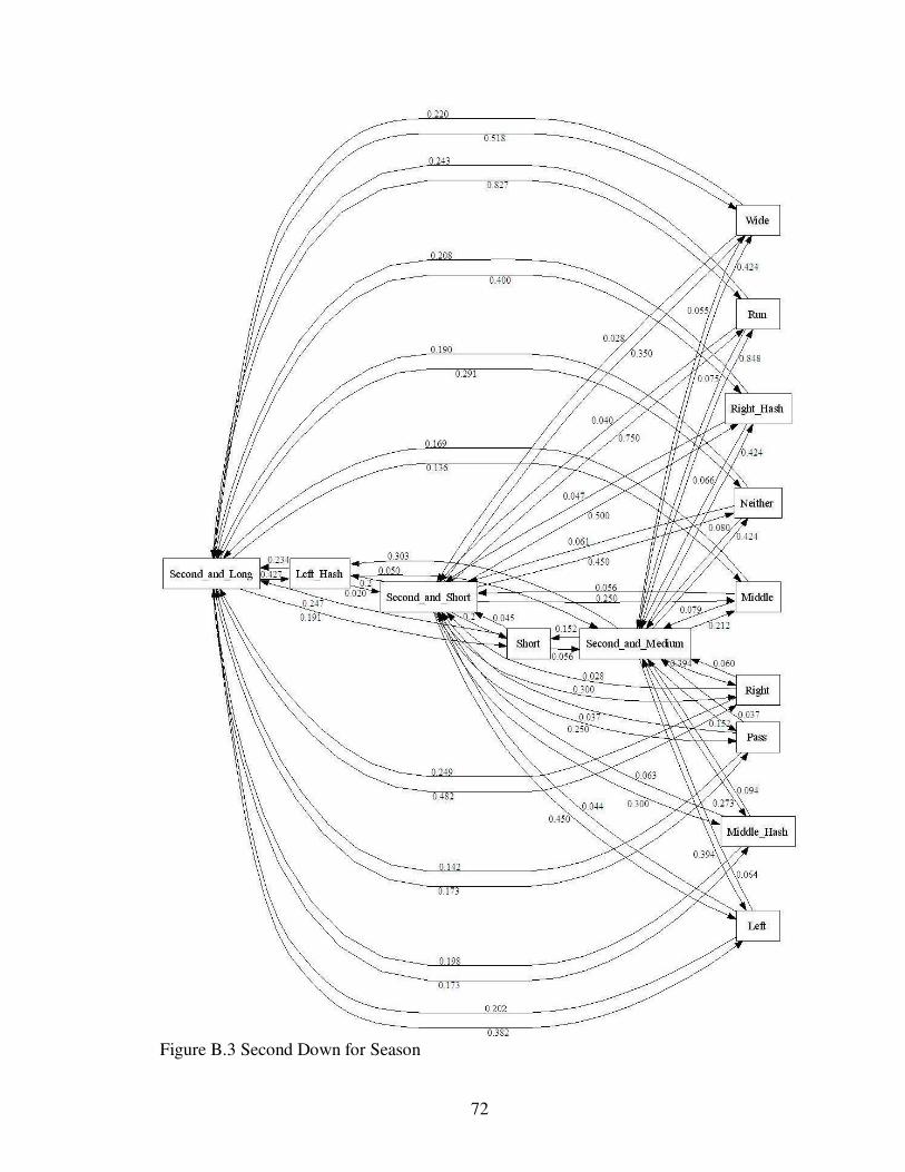
72
Figure B.3 Second Down for Season

73
Figure B.4 Third Down for Season

74
Figure B.5 Fourth Down for Season

75
Figure B.6 Sub graph for Season

76
APPENDIX C
DISTANCE MATRICES
This appendix contains the distance matrices calculated using the formula
discussed in chapter 4.

77
1st
and
Long
1st
and
Med
1st
and
Short
2nd
and
Long
2nd
and
Med
2nd
and
Short
3rd
and
Long
3rd
and
Med
3rd
and
Short
4th
and
Long
4th
and
Med
4th
and
Short
1st and Long
1st and Med
1st and Short
2nd and Long
2nd and Med
2nd and Short
3rd and Long
3rd and Med
3rd and Short
4th and Long
4th and Med
4th and Short
Left Hash 0.04 0 0 0.03 0.1 0.02 0.01 0 0.03 0.01 0 0.01
Mid. Hash 0.1 0 0 0.2 0.1 0.34 0.15 0.1 0.12 0.03 0 0.03
Right Hash 0.02 0 0 0.05 0 0.01 0.01 0 0.01 0.04 0 0.02
Run 0.07 0 0 0.04 0 0.01 0.03 0 0.01 0 0 0
Pass 0.08 0 0 0.14 0 0.07 0.06 0.1 0.01 0.09 0.1 0.07
Left 0.24 0 0 0.14 0.1 0.07 0.08 0 0.04 0.03 0 0.02
Middle 0.08 0 0.01 0.1 0 0.03 0.1 0 0.06 0 0 0.03
Right 0.13 0 0 0.05 0.1 0.03 0.06 0 0.05 0.03 0 0.06
Wide 0.07 0 0 0 0 0.02 0.01 0 0.03 0.02 0 0.02
Neither 0.15 0 0.01 0.01 0 0.07 0.12 0 0 0.02 0 0.03
Short 0.2 0 0 0.25 0 0.04 0.01 0 0.04 0.04 0 0.07
Left
Hash
Mid.
Hash
Right
Hash Run Pass Left Middle Right Wide Neither Short
1st and Long 0.1 0.05 0.05 0.1 0.1 0.1 0.073 0.17 0.11 0.0206 0.09
1st and Med 1 0 0 0.7 0.3 0 0 1 1 0 0
1st and Short 0.5 0 0.5 1 0 0 0.5 0.5 0.5 0.5 0
2nd and Long 0.2 0.17 0.03 0.2 0.2 0.3 0.239 0.02 0.11 0.0841 0.19
2nd and Med 0.45 0.27 0.17 0.2 0.2 0.4 0.038 0.36 0.08 0.1742 0.1
2nd and Short 0.2 0.37 0.17 0.1 0.1 0.2 0.083 0.3 0.02 0.2167 0.2
3rd and Long 0.17 0.24 0.07 0.1 0.1 0.3 0.155 0.41 0.22 0.3276 0.11
3rd and Med 0.04 0.21 0.17 0.3 0.3 0.2 0.125 0.04 0.38 0.2917 0.08
3rd and Short 0.25 0.17 0.08 0.1 0.1 0.3 0.208 0.54 0.29 0.0417 0.25
4th and Long 0.15 0.23 0.62 0.1 0.9 0.5 0 0.46 0.46 0.2308 0.31
4th and Med 0 0 0 0 0 0 0 0 0 0 0
4th and Short 0.1 0.2 0.1 0.2 0.2 0.3 0.2 0.47 0.03 0.3333 0.3
Left Hash 0.1 0.1 0 0.069 0.07 0.09 0.069 0.02
Mid. Hash 0 0 0.2 0.002 0.15 0 0 0
Right Hash 0.4 0.4 0.1 0.065 0.02 0.09 0.065 0.02
Run 0.15 0.1 0.05 0 0.053 0.02 0.05 0.017 0.07
Pass 0.08 0.04 0.12 0 0.022 0.02 0.17 0.0531 0.11
Left 0.09 0.04 0.05 0.1 0.1 0.06 0.0206 0.08
Middle 0.14 0.12 0.02 0 0 0 0 0
Right 0.1 0.11 0.01 0.1 0.1 0.08 0.1067 0.02
Wide 0.08 0 0.08 0 0 0.1 0 0.08
Neither 0.16 0.26 0.08 0.1 0.1 0 0.187 0.14
Short 0.07 0 0.07 0.2 0.2 0.1 0 0.05
Figure C.1 Distance between Colbert Heights and Season Average

78
1st
and
Long
1st
and
Med
1st
and
Short
2nd
and
Long
2nd
and
Med
2nd
and
Short
3rd
and
Long
3rd
and
Med
3rd
and
Short
4th
and
Long
4th
and
Med
4th
and
Short
1st and Long
1st and Med
1st and Short
2nd and Long
2nd and Med
2nd and Short
3rd and Long
3rd and Med
3rd and Short
4th and Long
4th and Med
4th and Short
Left Hash 0.16 0 0 0.14 0 0.02 0.05 0 0.03 0.01 0 0.02
Mid. Hash 0.11 0 0 0.05 0.1 0.06 0.1 0 0.02 0.03 0 0.03
Right Hash 0.06 0 0 0.13 0 0.05 0.1 0 0.05 0.04 0 0.03
Run 0.06 0 0 0.04 0 0.04 0.01 0 0.03 0 0 0.01
Pass 0.05 0 0 0.05 0 0.04 0.16 0 0.01 0.09 0 0.04
Left 0.04 0 0 0.06 0.1 0.04 0.07 0 0.04 0.03 0 0.02
Middle 0.17 0 0.01 0.03 0.1 0.06 0.18 0.1 0.06 0 0 0.03
Right 0.12 0 0 0.1 0.1 0.03 0.06 0 0 0.03 0 0.01
Wide 0.24 0 0 0.12 0 0.03 0.02 0 0.03 0.02 0 0.02
Neither 0.22 0 0.01 0.03 0.1 0.06 0.16 0.1 0.01 0.02 0 0.03
Short 0.03 0 0 0.13 0.1 0.04 0.16 0 0.06 0.04 0 0.03
Left
Hash
Mid.
Hash
Right
Hash Run Pass Left Middle Right Wide Neither Short
1st and Long 0.24 0.02 0.25 0 0 0 0.095 0.13 0.17 0.1397 0.03
1st and Med 1 0 0 0.7 0.3 0 0 1 1 0 0
1st and Short 0.5 0 0.5 1 0 0 0.5 0.5 0.5 0.5 0
2nd and Long 0.21 0.27 0.07 0.2 0.2 0.2 0.025 0.15 0.3 0.1535 0.14
2nd and Med 0.3 0.48 0.17 0.1 0.1 0.4 0.038 0.39 0.17 0.3258 0.15
2nd and Short 0.2 0.3 0.5 0.8 0.3 0.5 0.25 0.3 0.35 0.45 0.2
3rd and Long 0.01 0.2 0.21 0.1 0.1 0.1 0.067 0.01 0.31 0.228 0.08
3rd and Med 0.21 0.13 0.33 0.1 0.1 0.3 0.208 0.13 0.29 0.375 0.08
3rd and Short 0.25 0.67 0.42 0.1 0.1 0.3 0.208 0.54 0.29 0.5417 0.25
4th and Long 0.15 0.23 0.62 0.1 0.9 0.5 0 0.46 0.46 0.2308 0.31
4th and Med 0 0 1 0 1 1 0 0 1 0 0
4th and Short 0.6 0.2 0.4 0.3 0.3 0.3 0.2 0.47 0.53 0.3333 0.2
Left Hash 0.2 0.2 0.1 0.092 0.01 0 0.0917 0.1
Mid. Hash 0 0 0 0.115 0.1 0 0 0
Right Hash 0 0 0.1 0.087 0.02 0.11 0.087 0.02
Run 0.01 0.2 0.21 0 0.029 0.01 0.01 0.0573 0.07
Pass 0.15 0.1 0.25 0.1 0.04 0.01 0.24 0.1483 0.09
Left 0.11 0.16 0.27 0.1 0.1 0.28 0.1714 0.1
Middle 0.17 0.5 0.33 0.1 0.1 0 0 0
Right 0.1 0.04 0.14 0.1 0.1 0.08 0.0433 0.13
Wide 0.17 0 0.17 0 0 0.2 0 0.17
Neither 0.12 0.3 0.2 0.1 0.1 0.1 0.157 0.01
Short 0.32 0 0.32 0.3 0.3 0.3 0 0.3
Figure C.2 Distance between Addison and Season Average

79
1st
and
Long
1st
and
Med
1st
and
Short
2nd
and
Long
2nd
and
Med
2nd
and
Short
3rd
and
Long
3rd
and
Med
3rd
and
Short
4th
and
Long
4th
and
Med
4th
and
Short
1st and Long
1st and Med
1st and Short
2nd and Long
2nd and Med
2nd and Short
3rd and Long
3rd and Med
3rd and Short
4th and Long
4th and Med
4th and Short
Left Hash 0.15 0 0.04 0.03 0 0.02 0.04 0 0.01 0.01 0 0.03
Mid. Hash 0.01 0 0 0.14 0.1 0.06 0.08 0.1 0.04 0.03 0 0.03
Right Hash 0.03 0 0 0.02 0 0.03 0.08 0 0.01 0.04 0 0.01
Run 0.08 0 0.02 0.02 0.1 0.04 0.06 0 0 0.02 0 0.01
Pass 0.03 0 0 0.01 0 0.04 0.06 0 0.05 0.04 0 0.04
Left 0.06 0 0 0.02 0 0.04 0.06 0 0.09 0.05 0 0.02
Middle 0.08 0 0.01 0.01 0 0.02 0.02 0 0.06 0 0 0.04
Right 0.1 0 0.03 0.04 0.1 0.08 0.02 0 0.02 0.01 0 0.04
Wide 0.09 0 0.03 0.01 0 0.03 0.06 0 0.04 0.04 0 0
Neither 0.03 0 0.01 0.11 0 0.11 0.03 0 0.03 0.02 0 0.01
Short 0.12 0 0 0.18 0.1 0.1 0.05 0 0.06 0.04 0 0.03
Left
Hash
Mid.
Hash
Right
Hash Run Pass Left Middle Right Wide Neither Short
1st and Long 0.14 0.08 0.07 0 0 0.1 0.104 0.05 0.08 0.1372 0.05
1st and Med 0 0 0 0.3 0.3 0 0 0 0 0 0
1st and Short 0.5 0 0.5 0 0 0 0.5 0.5 0.5 0.5 0
2nd and Long 0.03 0.1 0.06 0 0 0 0.017 0.02 0.02 0.1371 0.12
2nd and Med 0.02 0.16 0.14 0.2 0.2 0.1 0.069 0.18 0 0.1472 0.15
2nd and Short 0.2 0.2 0 0.3 0.3 0.5 0 0.45 0.35 0.3 0.05
3rd and Long 0.27 0.04 0.23 0.4 0.4 0.1 0.045 0.06 0.13 0.0724 0.06
3rd and Med 0.54 0.21 0.33 0.3 0.3 0.3 0.125 0.46 0.38 0.2917 0.08
3rd and Short 0 0.17 0.17 0.2 0.2 0.4 0.208 0.21 0.21 0.2083 0
4th and Long 0.15 0.1 0.05 0.3 0.3 0.1 0 0.13 0.21 0.1026 0.31
4th and Med 0 0 1 0 1 1 0 0 1 0 0
4th and Short 0.4 0.3 0.1 0.3 0.3 0.2 0.3 0.53 0.03 0.1667 0.2
Left Hash 0 0 0 0.009 0 0.07 0.0089 0.06
Mid. Hash 0 0 0 0.073 0.08 0 0 0
Right Hash 0.1 0.1 0.1 0.11 0.02 0.02 0.1096 0.09
Run 0.07 0.06 0.01 0 0.011 0.03 0.02 0.044 0.03
Pass 0.06 0.05 0.11 0 0.044 0.03 0.01 0.0358 0.02
Left 0.01 0.09 0.1 0 0 0.03 0.0231 0.05
Middle 0.08 0.06 0.14 0 0 0 0 0
Right 0.09 0.08 0 0.1 0.1 0 0.0847 0.09
Wide 0.02 0 0.02 0 0 0.1 0 0.05
Neither 0.05 0.08 0.08 0 0 0.1 0.004 0.08
Short 0 0 0 0 0 0 0 0.02
Figure C.3 Distance between Cold Springs and Season Average

80
1st
and
Long
1st
and
Med
1st
and
Short
2nd
and
Long
2nd
and
Med
2nd
and
Short
3rd
and
Long
3rd
and
Med
3rd
and
Short
4th
and
Long
4th
and
Med
4th
and
Short
1st and Long
1st and Med
1st and Short
2nd and Long
2nd and Med
2nd and Short
3rd and Long
3rd and Med
3rd and Short
4th and Long
4th and Med
4th and Short
Left Hash 0.19 0 0 0.12 0 0.1 0.04 0 0.03 0.01 0 0.03
Mid. Hash 0.2 0 0 0.07 0.1 0.06 0.02 0.1 0.08 0.03 0 0.03
Right Hash 0.08 0 0.04 0.03 0.1 0.05 0.07 0 0 0.04 0 0.02
Run 0.1 0 0.03 0.1 0 0.05 0 0 0.03 0 0 0
Pass 0.24 0 0 0.01 0.1 0.04 0.2 0 0.01 0.09 0 0.04
Left 0.17 0 0 0.01 0.2 0.04 0.14 0 0.04 0.03 0 0.02
Middle 0.08 0 0.07 0.17 0 0.1 0.05 0 0.06 0 0 0.03
Right 0.15 0 0 0.06 0.1 0.02 0.04 0 0 0.03 0 0.01
Wide 0.03 0 0 0 0.1 0.03 0.07 0 0.03 0.02 0 0.03
Neither 0.17 0 0.05 0.13 0 0.05 0.01 0 0.07 0.02 0 0.03
Short 0.26 0 0 0.08 0.1 0.04 0.09 0 0.03 0.04 0 0.05
Left
Hash
Mid.
Hash
Right
Hash Run Pass Left Middle Right Wide Neither Short
1st and Long 0.03 0.01 0.01 0.1 0.1 0.1 0.069 0.02 0.21 0.0871 0.12
1st and Med 1 0 0 0.7 0.3 0 0 1 1 0 0
1st and Short 0.5 0 0.5 0 0 0 0.5 0.5 0.5 0.5 0
2nd and Long 0.14 0.03 0.17 0.1 0.1 0 0.136 0.09 0.05 0.0052 0.05
2nd and Med 0.3 0.27 0.58 0.3 0.3 0.4 0.038 0.39 0.33 0.1742 0.15
2nd and Short 0.47 0.03 0.5 0.3 0.3 0.5 0.417 0.03 0.02 0.2167 0.2
3rd and Long 0.01 0.09 0.1 0.3 0.3 0.5 0.511 0.01 0.2 0.3391 0.14
3rd and Med 0.04 0.29 0.33 0.3 0.3 0.3 0.125 0.46 0.13 0.2083 0.08
3rd and Short 0.25 0.33 0.58 0.1 0.1 0.3 0.208 0.54 0.29 0.4583 0.75
4th and Long 0.15 0.23 0.62 0.1 0.9 0.5 0 0.46 0.46 0.2308 0.31
4th and Med 0 0 1 0 1 1 0 0 1 0 0
4th and Short 0.4 0.2 0.6 0.3 0.3 0.3 0.2 0.47 0.47 0.3333 0.8
Left Hash 0.1 0.1 0 0.214 0.18 0.14 0.2136 0.07
Mid. Hash 0.2 0.2 0.2 0.177 0.02 0 0 0
Right Hash 0 0 0.2 0.024 0.19 0.17 0.0242 0.19
Run 0.08 0.03 0.05 0.1 0.142 0 0.17 0.1383 0.03
Pass 0.05 0.15 0.1 0 0.022 0.04 0 0.1642 0.16
Left 0.01 0.07 0.06 0.1 0.1 0.12 0.0542 0.07
Middle 0.15 0.02 0.16 0 0 0 0 0
Right 0.22 0.01 0.24 0 0 0.24 0.0138 0.25
Wide 0.03 0 0.03 0.1 0.1 0.1 0 0.08
Neither 0.16 0.14 0.04 0.1 0.1 0.1 0.176 0.04
Short 0.26 0 0.26 0.1 0.1 0.3 0 0.28
Figure C.4 Distance between Clements and Season Average

81
1st
and
Long
1st
and
Med
1st
and
Short
2nd
and
Long
2nd
and
Med
2nd
and
Short
3rd
and
Long
3rd
and
Med
3rd
and
Short
4th
and
Long
4th
and
Med
4th
and
Short
1st and Long
1st and Med
1st and Short
2nd
and Long
2nd
and Med
2nd
and Short
3rd and Long
3rd and Med
3rd and Short
4th and Long
4th and Med
4th and Short
Left Hash 0.22 0 0 0.18 0 0.02 0.02 0.1 0.03 0.01 0 0.03
Mid. Hash 0.05 0 0 0.05 0.2 0.06 0.15 0.1 0.17 0.03 0 0.03
Right Hash 0.03 0 0 0.06 0 0.05 0.02 0.1 0.1 0.04 0 0.03
Run 0.09 0 0 0 0 0.04 0.03 0.1 0.05 0 0 0.03
Pass 0.1 0 0 0.26 0 0.04 0.12 0 0.01 0.09 0 0.04
Left 0.04 0 0 0.09 0 0.04 0.02 0.1 0.02 0.03 0 0.02
Middle 0.26 0 0.01 0.23 0.1 0.06 0.1 0 0.14 0 0 0.03
Right 0.11 0 0 0.12 0 0.03 0.01 0 0.05 0.03 0 0.04
Wide 0.13 0 0 0.06 0 0.03 0.08 0.1 0.03 0.02 0 0.03
Neither 0.14 0 0.01 0.18 0 0.06 0.12 0 0.18 0.02 0 0.03
Short 0.15 0 0 0.14 0.1 0.04 0.09 0.1 0.17 0.04 0 0.03
Left
Hash
Mid.
Hash
Right
Hash Run Pass Left Middle Right Wide Neither Short
1st and Long 0.16 0.07 0.23 0.1 0.1 0.2 0.129 0.04 0.02 0.1547 0.17
1st and Med 1 0 0 0.7 0.3 0 0 1 1 0 0
1st and Short 0.5 0 0.5 1 0 0 0.5 0.5 0.5 0.5 0
2nd
and Long 0.21 0.08 0.13 0 0 0.2 0.045 0.15 0.12 0.0182 0.1
2nd
and Med 0.03 0.06 0.09 0.2 0.2 0.1 0.121 0.06 0.24 0.0909 0.15
2nd
and Short 0.2 0.3 0.5 0.8 0.3 0.5 0.25 0.3 0.35 0.45 0.2
3rd and Long 0.07 0.24 0.17 0.2 0.2 0.1 0.155 0.06 0.47 0.3276 0.14
3rd and Med 0.14 0.21 0.07 0.3 0.3 0.3 0.125 0.14 0.18 0.2917 0.12
3rd and Short 0.25 0.08 0.33 0.1 0.1 0.1 0.042 0.04 0.29 0.0417 0.25
4th and Long 0.15 0.23 0.62 0.1 0.9 0.5 0 0.46 0.46 0.2308 0.31
4th and Med 0 0 1 0 1 1 0 0 1 0 0
4th and Short 0.4 0.2 0.4 0.7 0.3 0.3 0.2 0.53 0.47 0.3333 0.2
Left Hash 0.1 0.1 0 0.08 0.05 0.09 0.0805 0.01
Mid. Hash 0 0 0.1 0.052 0.1 0 0 0
Right Hash 0.3 0.3 0 0.055 0.04 0.01 0.0553 0.05
Run 0.01 0.12 0.13 0.1 0.094 0.02 0.11 0.1868 0.08
Pass 0.19 0.05 0.24 0.4 0.022 0.37 0.19 0.0358 0.22
Left 0.02 0.1 0.09 0.3 0.3 0.13 0.0859 0.05
Middle 0.11 0.01 0.13 0 0 0 0 0
Right 0.03 0.1 0.08 0.1 0.1 0.01 0.1041 0.09
Wide 0.01 0 0.01 0.2 0.2 0 0 0.05
Neither 0.05 0.09 0.12 0 0 0 0.079 0.08
Short 0.09 0 0.09 0.3 0.3 0.1 0 0.12
Figure C.5 Distance between Sheffield and Season Average

82
1st
and
Long
1st
and
Med
1st
and
Short
2nd
and
Long
2nd
and
Med
2nd
and
Short
3rd
and
Long
3rd
and
Med
3rd
and
Short
4th
and
Long
4th
and
Med
4th
and
Short
1st and Long
1st and Med
1st and Short
2nd
and Long
2nd
and Med
2nd
and Short
3rd and Long
3rd and Med
3rd and Short
4th and Long
4th and Med
4th and Short
Left Hash 0.05 0.1 0 0.01 0 0.02 0.02 0.1 0.01 0.03 0 0.04
Mid. Hash 0.02 0 0 0.09 0.1 0.06 0 0.1 0.08 0.03 0 0.11
Right Hash 0.1 0 0 0.01 0.1 0.15 0.12 0.1 0.05 0.04 0 0.03
Run 0 0 0 0.02 0 0 0.02 0 0.02 0 0 0.01
Pass 0.06 0.1 0 0.09 0 0.08 0.16 0 0.01 0.03 0 0.08
Left 0.11 0 0 0.01 0 0.08 0.02 0 0 0.01 0 0.02
Middle 0.04 0 0.01 0.17 0.1 0.06 0.1 0 0.06 0 0 0.47
Right 0.07 0.1 0 0.03 0 0.03 0.04 0.1 0.05 0.03 0 0.02
Wide 0.02 0.1 0 0.04 0 0.02 0.08 0 0.03 0.02 0 0.02
Neither 0.05 0 0.01 0.03 0.1 0.06 0.01 0.1 0.07 0.02 0 0.19
Short 0.15 0 0 0.08 0 0.12 0.08 0 0.03 0.04 0 0.03
Left
Hash
Mid.
Hash
Right
Hash Run Pass Left Middle Right Wide Neither Short
1st and Long 0.24 0.02 0.22 0.1 0.1 0 0.138 0.1 0.11 0.1101 0
1st and Med 0 0 0 0.2 0.2 0 0 0 0 0 0
1st and Short 0.5 0 0.5 1 0 0 0.5 0.5 0.5 0.5 0
2nd
and Long 0.17 0.03 0.2 0.2 0.2 0.2 0.136 0.08 0.08 0.0909 0.01
2nd
and Med 0.3 0.27 0.58 0.3 0.3 0.1 0.212 0.11 0.08 0.4242 0.35
2nd
and Short 0.13 0.3 0.17 0.4 0.4 0.6 0.25 0.3 0.02 0.45 0.47
3rd and Long 0.42 0.01 0.43 0.1 0.1 0.3 0.155 0.09 0.28 0.0776 0.36
3rd and Med 0.46 0.29 0.17 0.3 0.3 0.7 0.125 0.54 0.13 0.2083 0.08
3rd and Short 0.75 0.33 0.42 0.1 0.1 0.7 0.208 0.46 0.29 0.4583 0.75
4th and Long 0.85 0.23 0.62 0.1 0.1 0.5 0 0.46 0.46 0.2308 0.69
4th and Med 0 0 1 0 1 1 0 0 1 0 0
4th and Short 0.27 0.13 0.4 0.3 0.3 0.1 0.133 0.2 0.13 0.3333 0.2
Left Hash 0.1 0.1 0.2 0.065 0.1 0.12 0.0652 0.18
Mid. Hash 0.1 0.1 0.3 0.198 0.07 0 0 0
Right Hash 0.1 0.1 0.3 0.198 0.15 0.24 0.1981 0.04
Run 0.2 0.02 0.19 0.2 0.155 0.06 0.06 0.1167 0.06
Pass 0.24 0.03 0.21 0 0.022 0.05 0.08 0.0465 0.13
Left 0.21 0 0.21 0 0 0.26 0.0113 0.25
Middle 0.69 0.21 0.47 0 0 0 0 0
Right 0.23 0.05 0.18 0.2 0.2 0.22 0.0456 0.17
Wide 0.12 0 0.12 0.1 0.1 0.1 0 0.12
Neither 0.05 0.19 0.26 0.1 0.1 0.3 0.324 0.01
Short 0.41 0 0.41 0.2 0.2 0.5 0 0.47
Figure C.6 Distance between Tanner and Season Average

83
1st
and
Long
1st
and
Med
1st
and
Short
2nd
and
Long
2nd
and
Med
2nd
and
Short
3rd
and
Long
3rd
and
Med
3rd
and
Short
4th
and
Long
4th
and
Med
4th
and
Short
1st and Long
1st and Med
1st and Short
2nd
and Long
2nd
and Med
2nd
and Short
3rd and Long
3rd and Med
3rd and Short
4th and Long
4th and Med
4th and Short
Left Hash 0.01 0 0 0.02 0 0.03 0.06 0.1 0.02 0.01 0 0.02
Mid. Hash 0.12 0 0 0.17 0.1 0.06 0.05 0 0.08 0.15 0 0.06
Right Hash 0.01 0 0 0.04 0 0.05 0 0 0 0.01 0 0
Run 0.03 0 0 0.06 0.1 0.02 0.01 0 0 0 0 0.01
Pass 0.12 0 0 0.03 0 0.04 0.02 0.1 0.01 0.08 0 0.01
Left 0.06 0 0 0.08 0 0.04 0.04 0 0.04 0 0 0.04
Middle 0.14 0 0.01 0.07 0.1 0.06 0.1 0.1 0.14 0 0 0.03
Right 0.04 0 0 0.05 0 0.01 0.01 0 0.02 0.07 0 0
Wide 0 0 0 0 0 0 0.07 0 0 0.02 0 0.02
Neither 0.01 0 0.01 0.05 0.1 0.06 0.07 0.1 0.03 0.08 0 0.02
Short 0.2 0 0 0.25 0 0.04 0.09 0 0.06 0.16 0 0.03
Left
Hash
Mid.
Hash
Right
Hash Run Pass Left Middle Right Wide Neither Short
1st and Long 0.12 0.07 0.18 0 0 0 0.022 0.03 0.11 0.0013 0.11
1st and Med 1 0 0 0.7 0.3 0 0 1 1 0 0
1st and Short 0.5 0 0.5 1 0 0 0.5 0.5 0.5 0.5 0
2nd
and Long 0.16 0.04 0.13 0 0 0.1 0.084 0.01 0.01 0.0278 0.02
2nd
and Med 0.3 0.27 0.58 0.3 0.3 0.1 0.212 0.11 0.08 0.4242 0.35
2nd
and Short 0.8 0.3 0.5 0.3 0.3 0.5 0.25 0.7 0.65 0.45 0.2
3rd and Long 0.01 0.13 0.12 0 0 0.2 0.155 0.01 0.35 0.2165 0.14
3rd and Med 0.46 0.04 0.42 0.5 0.5 0.2 0.125 0.29 0.13 0.2083 0.08
3rd and Short 0.08 0.33 0.25 0.1 0.1 0.3 0.458 0.13 0.04 0.2083 0.25
4th and Long 0.15 0.27 0.12 0.1 0.1 0.3 0 0.29 0.46 0.2692 0.19
4th and Med 0 0 1 0 1 1 0 0 1 0 0
4th and Short 0.07 0.13 0.07 0 0 0.4 0.2 0.2 0.2 0 0.2
Left Hash 0.2 0.2 0.2 0.039 0.2 0.18 0.0393 0.14
Mid. Hash 0.2 0.2 0.2 0.198 0.01 0 0 0
Right Hash 0.1 0.1 0 0.003 0.03 0.02 0.003 0.02
Run 0.02 0.08 0.1 0 0.025 0.04 0.07 0.0495 0.02
Pass 0.32 0.07 0.26 0.1 0.022 0.12 0.04 0.0532 0.09
Left 0.18 0.01 0.17 0.1 0.1 0.16 0.0217 0.18
Middle 0.11 0.21 0.33 0 0 0 0 0
Right 0.04 0.02 0.06 0 0 0.05 0.0233 0.07
Wide 0.12 0 0.12 0 0 0.1 0 0.11
Neither 0.08 0.07 0.12 0.1 0.1 0.1 0.07 0.02
Short 0.33 0 0.33 0 0 0.3 0 0.35
Figure C.7 Distance between Hatton and Season Average

84
1st
and
Long
1st
and
Med
1st
and
Short
2nd
and
Long
2nd
and
Med
2nd
and
Short
3rd
and
Long
3rd
and
Med
3rd
and
Short
4th
and
Long
4th
and
Med
4th
and
Short
1st and Long
1st and Med
1st and Short
2nd
and Long
2nd
and Med
2nd
and Short
3rd and Long
3rd and Med
3rd and Short
4th and Long
4th and Med
4th and Short
Left Hash 0.04 0 0 0.08 0 0.02 0.09 0.1 0.03 0.05 0 0.03
Mid. Hash 0.05 0 0 0.11 0.1 0.02 0.19 0.1 0 0.03 0 0.03
Right Hash 0.04 0 0 0.05 0.1 0.03 0.04 0 0.01 0.08 0 0.01
Run 0.06 0 0 0 0 0.01 0.09 0 0.01 0 0 0
Pass 0.07 0 0 0.14 0 0.05 0.09 0 0.01 0.27 0 0.04
Left 0.09 0 0 0.07 0 0.05 0.08 0 0.01 0.06 0 0.02
Middle 0.09 0 0.01 0.06 0.1 0.06 0.12 0 0.06 0 0 0.08
Right 0.01 0 0 0.02 0 0.02 0.05 0 0.04 0.06 0 0.04
Wide 0.07 0 0 0.09 0.1 0.01 0.01 0.1 0.05 0.09 0 0.03
Neither 0 0 0.01 0.13 0 0.01 0.16 0 0.01 0.02 0 0.02
Short 0.04 0 0 0.14 0.1 0.07 0.09 0.1 0.06 0.07 0 0.03
Left
Hash
Mid.
Hash
Right
Hash Run Pass Left Middle Right Wide Neither Short
1st and Long 0.05 0.01 0.04 0 0 0.1 0.05 0 0.07 0.0524 0.01
1st and Med 1 0 0 0.7 0.3 0 0 1 1 0 0
1st and Short 0.5 0 0.5 1 0 0 0.5 0.5 0.5 0.5 0
2nd
and Long 0.07 0.07 0 0.2 0.2 0.1 0.036 0.12 0.28 0.1909 0.09
2nd
and Med 0.03 0.39 0.42 0.2 0.2 0.3 0.212 0.06 0.42 0.2424 0.18
2nd
and Short 0.2 0.03 0.17 0.1 0.1 0.2 0.25 0.03 0.02 0.1167 0.13
3rd and Long 0.33 0.26 0.07 0.4 0.4 0.1 0.095 0.22 0.16 0.2974 0.14
3rd and Med 0.46 0.21 0.67 0.3 0.3 0.3 0.125 0.46 0.63 0.2917 0.92
3rd and Short 0.08 0 0.08 0.1 0.1 0 0.208 0.21 0.38 0.125 0.25
4th and Long 0.1 0.23 0.13 0.1 0.1 0 0 0.04 0.29 0.2308 0.06
4th and Med 0 0 1 0 1 1 0 0 1 0 0
4th and Short 0.4 0.2 0.6 0.3 0.3 0.3 0.8 0.53 0.47 0.6667 0.2
Left Hash 0 0 0 0.077 0.1 0.08 0.0768 0
Mid. Hash 0.1 0.1 0.1 0.052 0.06 0 0 0
Right Hash 0.1 0.1 0 0.002 0.05 0 0.0019 0
Run 0.1 0.06 0.04 0 0.015 0.02 0.03 0.0288 0
Pass 0.05 0.06 0.11 0 0.022 0.03 0.12 0.0733 0.04
Left 0.07 0.03 0.1 0.1 0.1 0.05 0.0152 0.03
Middle 0.2 0.12 0.08 0 0 0 0 0
Right 0.06 0.07 0.01 0 0 0.07 0.0706 0
Wide 0.07 0 0.07 0 0 0.1 0 0.07
Neither 0.12 0.08 0.02 0.1 0.1 0 0.046 0.07
Short 0.09 0 0.09 0.1 0.1 0 0 0
Figure C.8 Distance between Red Bay and Season Average

85
1st
and
Long
1st
and
Med
1st
and
Short
2nd
and
Long
2nd
and
Med
2nd
and
Short
3rd
and
Long
3rd
and
Med
3rd
and
Short
4th
and
Long
4th
and
Med
4th
and
Short
1st and Long
1st and Med
1st and Short
2nd
and Long
2nd
and Med
2nd
and Short
3rd and Long
3rd and Med
3rd and Short
4th and Long
4th and Med
4th and Short
Left Hash 0.02 0 0 0 0 0.02 0 0 0.02 0.01 0 0.03
Mid. Hash 0.1 0 0 0.1 0.1 0.06 0.05 0 0.02 0.03 0 0.03
Right Hash 0.06 0 0 0.03 0.1 0.04 0.06 0 0.05 0.01 0 0.03
Run 0.05 0 0 0.07 0 0.01 0.03 0 0.01 0 0 0.03
Pass 0.06 0 0 0.14 0 0.03 0.15 0 0.01 0.02 0.1 0.04
Left 0.02 0 0 0.04 0.1 0.05 0 0 0.04 0.01 0 0.02
Middle 0.02 0 0.01 0.06 0 0.06 0.1 0.1 0.17 0 0 0.03
Right 0.1 0 0 0.01 0 0.03 0.08 0 0.05 0.03 0 0.04
Wide 0.07 0 0 0.03 0 0.04 0.01 0 0.03 0.01 0 0.03
Neither 0.05 0 0.01 0.06 0 0.06 0.05 0 0.06 0.02 0 0.03
Short 0.07 0 0 0.09 0.1 0.04 0.24 0 0.06 0.04 0 0.03
Left
Hash
Mid.
Hash
Right
Hash Run Pass Left Middle Right Wide Neither Short
1st and Long 0.03 0.03 0.01 0 0 0 0.033 0.06 0.11 0.0476 0.06
1st and Med 1 0 0 0.7 0.3 0 0 1 1 0 0
1st and Short 0.5 0 0.5 1 0 0 0.5 0.5 0.5 0.5 0
2nd
and Long 0.01 0.08 0.07 0.2 0.2 0 0.053 0.02 0.02 0.0424 0.02
2nd
and Med 0.7 0.27 0.42 0.2 0.2 0.4 0.288 0.11 0.08 0.0758 0.15
2nd
and Short 0.2 0.3 0.5 0.3 0.3 0.6 0.25 0.3 0.65 0.45 0.2
3rd and Long 0.04 0.1 0.14 0.2 0.2 0.1 0.155 0.23 0.04 0.1847 0.15
3rd and Med 0.04 0.29 0.33 0.3 0.3 0.3 0.375 0.04 0.13 0.2083 0.08
3rd and Short 0.25 0.17 0.42 0.1 0.1 0.3 0.792 0.46 0.29 0.5417 0.25
4th and Long 0.15 0.23 0.38 0.1 0.1 0.5 0 0.46 0.54 0.2308 0.31
4th and Med 0 0 0 0 0 0 0 0 0 0 0
4th and Short 0.4 0.2 0.4 0.7 0.3 0.3 0.2 0.53 0.47 0.3333 0.2
Left Hash 0.1 0.1 0.1 0.051 0.06 0.04 0.0512 0.09
Mid. Hash 0 0 0.1 0.102 0.05 0 0 0
Right Hash 0 0 0.2 0.107 0.06 0.17 0.1072 0.06
Run 0.05 0 0.05 0 0.001 0.02 0.08 0.017 0.06
Pass 0.12 0.01 0.13 0.1 0.022 0.07 0.1 0.0213 0.08
Left 0.11 0.07 0.18 0 0 0.17 0.0542 0.12
Middle 0.13 0.12 0.25 0 0 0 0 0
Right 0.05 0.02 0.07 0 0 0.03 0.0172 0.05
Wide 0.05 0 0.05 0 0 0 0 0.04
Neither 0.08 0.04 0.13 0 0 0.1 0.016 0.04
Short 0.09 0 0.09 0 0 0.1 0 0.12
Figure C.9 Distance between Coffee and Season Average

86
1st
and
Long
1st
and
Med
1st
and
Short
2nd
and
Long
2nd
and
Med
2nd
and
Short
3rd
and
Long
3rd
and
Med
3rd
and
Short
4th
and
Long
4th
and
Med
4th
and
Short
1st and Long
1st and Med
1st and Short
2nd
and Long
2nd
and Med
2nd
and Short
3rd and Long
3rd and Med
3rd and Short
4th and Long
4th and Med
4th and Short
Left Hash 0.01 0 0 0.03 0 0.02 0.09 0 0.04 0.01 0 0.04
Mid. Hash 0.13 0 0 0.09 0.1 0.06 0 0.1 0.06 0.03 0 0.03
Right Hash 0.15 0 0 0.1 0 0.02 0.07 0 0.02 0.04 0 0.03
Run 0.07 0 0 0.09 0 0 0.02 0 0.02 0 0 0.01
Pass 0.07 0 0 0.04 0 0.04 0 0 0.08 0.09 0 0.05
Left 0.06 0 0 0.03 0.1 0.04 0.01 0 0.11 0.03 0 0.02
Middle 0.26 0 0.01 0.23 0 0.04 0.1 0 0.06 0 0 0.03
Right 0.02 0 0 0.02 0 0.03 0.09 0 0.02 0.03 0 0.1
Wide 0.09 0 0 0.1 0.1 0.03 0 0 0.1 0.02 0 0.03
Neither 0.07 0 0.01 0.18 0 0 0.01 0 0 0.02 0 0.03
Short 0.24 0 0 0.25 0.1 0.04 0.09 0 0.06 0.04 0 0.13
Left
Hash
Mid.
Hash
Right
Hash Run Pass Left Middle Right Wide Neither Short
1st and Long 0.05 0.07 0.12 0.1 0.1 0 0.057 0.03 0.05 0.0596 0.11
1st and Med 1 0 0 0.7 0.3 0 0 1 1 0 0
1st and Short 0.5 0 0.5 1 0 0 0.5 0.5 0.5 0.5 0
2nd
and Long 0.06 0.01 0.05 0 0 0.1 0.227 0.12 0.34 0.2545 0.08
2nd
and Med 0.2 0.27 0.08 0.2 0.2 0.4 0.288 0.11 0.42 0.0758 0.35
2nd
and Short 0.2 0.3 0.5 0.3 0.3 0.5 0.75 0.3 0.35 0.55 0.2
3rd and Long 0.33 0.01 0.32 0.1 0.1 0 0.345 0.34 0.03 0.1724 0.14
3rd and Med 0.54 0.21 0.33 0.3 0.3 0.3 0.125 0.46 0.38 0.2917 0.08
3rd and Short 0.08 0 0.08 0.3 0.3 0.3 0.208 0.13 0.38 0.125 0.25
4th and Long 0.15 0.23 0.62 0.1 0.9 0.5 0 0.46 0.46 0.2308 0.31
4th and Med 0 0 1 0 1 1 0 0 1 0 0
4th and Short 0.1 0.2 0.1 0.2 0.2 0.3 0.2 0.47 0.03 0.3333 0.3
Left Hash 0.1 0.1 0 0.061 0.05 0.07 0.0607 0.01
Mid. Hash 0.1 0.1 0 0.055 0.07 0 0 0
Right Hash 0.1 0.1 0.1 0.177 0.06 0.12 0.1769 0.05
Run 0.06 0.02 0.04 0.1 0.104 0.02 0.09 0.1425 0.05
Pass 0.14 0.06 0.08 0.1 0.069 0.15 0.07 0.0176 0.05
Left 0.02 0.02 0.04 0.2 0.2 0.05 0.0337 0.02
Middle 0.01 0.11 0.13 0.1 0.1 0 0 0
Right 0 0.04 0.04 0.1 0.1 0.02 0.0433 0.03
Wide 0.03 0 0.03 0.1 0.1 0 0 0.03
Neither 0.02 0.15 0.12 0 0 0.1 0.079 0.02
Short 0.07 0 0.07 0.2 0.2 0.1 0 0.05
Figure C.10 Distance between Vincent and Season Average

87
1st
and
Long
1st
and
Med
1st
and
Short
2nd
and
Long
2nd
and
Med
2nd
and
Short
3rd
and
Long
3rd
and
Med
3rd
and
Short
4th
and
Long
4th
and
Med
4th
and
Short
1st and Long
1st and Med
1st and Short
2nd
and Long
2nd
and Med
2nd
and Short
3rd and Long
3rd and Med
3rd and Short
4th and Long
4th and Med
4th and Short
Left Hash 0.06 0 0.02 0.03 0.1 0 0.01 0 0 0.02 0 0
Mid. Hash 0.11 0 0 0.14 0 0.16 0.2 0 0.05 0.05 0 0.05
Right Hash 0.04 0 0 0.02 0 0.03 0.1 0 0.03 0.01 0 0.03
Run 0.02 0 0.01 0.02 0 0.05 0.09 0 0.02 0.01 0 0.02
Pass 0.01 0 0 0.07 0 0.01 0.01 0 0.04 0.04 0 0.04
Left 0.1 0 0 0.02 0.1 0.02 0.13 0 0.04 0.02 0 0.03
Middle 0.16 0 0 0.02 0 0.08 0.15 0 0.05 0 0 0.01
Right 0.11 0 0.02 0.06 0.1 0.04 0 0 0.02 0.01 0 0.02
Wide 0.08 0 0.02 0.02 0.1 0 0.05 0 0.01 0.01 0 0.02
Neither 0.16 0 0 0.06 0 0.12 0.18 0 0.04 0.02 0 0
Short 0.01 0 0 0.02 0 0.02 0.04 0.1 0.02 0.04 0 0.06
Left
Hash
Mid.
Hash
Right
Hash Run Pass Left Middle Right Wide Neither Short
1st and Long 0.05 0.02 0.03 0 0 0 0.138 0.15 0.12 0.1514 0.03
1st and Med 1 0 0 1 0 0 0 1 1 0 0
1st and Short 1 0 0 1 0 0 0 1 1 0 0
2nd
and Long 0.06 0.15 0.1 0.1 0.1 0 0.105 0.06 0 0.0286 0.02
2nd
and Med 0.25 0.33 0.07 0.1 0.1 0.4 0.018 0.44 0.15 0.1455 0.01
2nd
and Short 0 0.24 0.24 0.2 0.2 0.4 0.286 0.1 0.19 0.381 0.19
3rd and Long 0.33 0.25 0.08 0.4 0.4 0.2 0.071 0.28 0.1 0.2323 0.13
3rd and Med 0.19 0.11 0.08 0.1 0.1 0.1 0.111 0.19 0.44 0.2222 0.22
3rd and Short 0.04 0.13 0.17 0.2 0.2 0.3 0.125 0.13 0.08 0.1667 0.08
4th and Long 0.25 0.33 0.08 0.3 0.3 0.2 0 0.17 0.08 0.3333 0.25
4th and Med 0 0 1 0 1 1 0 0 1 0 0
4th and Short 0.25 0.25 0 0.3 0.3 0.3 0.25 0 0 0.25 0.25
Left Hash 0.1 0.1 0 0.115 0.09 0.06 0.1147 0.05
Mid. Hash 0 0 0.1 0.138 0.07 0 0 0
Right Hash 0.2 0.2 0.2 0.125 0.03 0.07 0.1253 0.05
Run 0.07 0.05 0.02 0.1 0.075 0.03 0.06 0.0538 0.01
Pass 0.08 0.02 0.1 0.1 0.01 0.08 0.1 0.0521 0.05
Left 0.03 0.03 0.06 0.1 0.1 0.01 0.0453 0.05
Middle 0.19 0.3 0.11 0 0 0 0 0
Right 0.03 0 0.03 0.1 0.1 0.03 0.0007 0.03
Wide 0.02 0 0.02 0 0 0.1 0 0.06
Neither 0.12 0.23 0.1 0 0.1 0.1 0.094 0.04
Short 0.01 0 0.01 0.1 0.1 0 0 0.03
Figure C.11 Distance between Close Wins and Close Losses

88
APPENDIX D
GOULD ACCESSIBILITY INDEX
This appendix contains the data for the eigenvalues, eigenvectors, and Gould
Accessibility Indices as discussed in section 5.5. These were calculated using Matlab.
Colbert Heights Addison Cold Springs Clements Sheffield Tanner Hatton Red Bay
4.00000 + 0i 4 4.00952 + 0i 4 4 4 4 4
1.40513 + 0i 1.582017 1.29508 + 0i 1.612698 1.35704 1.266589 1.05964 1.49206
0.99754 + 0i 0.854547 0.73934 + 0i 0.803309 0.855117 1.030334 1.05630 0.78209
0.47214 + 0i 0.453191 0.50168 + 0i 0.529 0.466826 0.663762 0.66984 0.46067
0.41128 + 0i -0.70216 0.31994 + 0.01595i 0.209488 0.248734 0.345362 0.47560 0.43040
-0.97608 + 0i -0.59447 0.31994 - 0.01595i 0.084835 0.004667 0.319283 -0.79785 0.29451
-0.68917 + 0.04454i -0.41852 0.09721 + 0i 0.049154 -0.00546 -0.87149 -0.65155 -0.93946
-0.68918 - 0.04454i 0.137117 0.00225 + 0i 0.007021 -0.07851 0.023681 -0.46823 -0.67968
-0.52528 + 0i 0.066232 0 + 0i -0.26133 -0.30097 0 0.17746 -0.63581
-0.42015 + 0i 0.004211 -0.15989 + 0i -0.3479 -0.622 -0.15987 -0.29657 -0.53635
0.20378 + 0i -0.04535 -0.20055 + 0i -0.41281 -0.50005 -0.21666 -0.13432 -0.40658
-0.20337 + 0i -0.10619 -0.31674 + 0i -0.56468 -0.45893 -0.39709 -0.09217 -0.29376
0.05442 + 0i -0.2768 -0.40141 + 0i -0.76582 -0.96646 -0.52716 0.00184 0.06908
-0.04165 + 0i -0.95383 -0.50662 + 0i -0.94297 -1 -0.47674 0 -0.0389
-0 + 0i -1 -0.65854 + 0i -1 -1 -1 0 0
0.00060 + 0i -1 -1.06740 + 0i -1 -1 -1 -1 0.001744
-1 + 0i -1 -0.97382 + 0i 0 -1 0 -1 -1
-0.99999 + 0i -1 -0.99999 + 0i 0 0 0 -1 -1
-1 + 0i 0 -1 + 0i -1 0 -1 -1 -1
-1 + 0i 0 -1 + 0i -1 0 -1 -1 -1
0 + 0i 0 0 + 0i 0 0 -1 0 0
0 + 0i 0 -0 + 0i 0 0 0 0 0
0 + 0i 0 0 + 0i 0 0 0 0 0
Figure D.1 Eigenvalues Part 1

89
Coffee Vincent Blowout Wins Close Wins Close Losses Blowout Losses Season
4 4 4 3.98508 + 0i 4 4 4.001181
1.67246 1.324199 1.330887 1.21259 + 0i 1.328554 1.128717 1.127771
0.78357 0.797664 0.573404 0.73272 + 0i 0.540617 0.762446 0.586991
0.47117 0.553641 -0.95223 -0.94973 + 0i -0.92964 -0.96168 -0.95267
0.28485 -0.97655 0.377844 -1.01609 + 0i 0.390524 0.413121 -1.00213
-0.94311 -0.72395 0.332111 0.40648 + 0i -0.54802 -0.64974 -0.47483
-0.71818 -0.62445 -0.53234 -0.59586 + 0i -0.4773 -0.5038 -0.40131
-0.65028 -0.41995 0.205323 -0.47545 + 0i -0.36335 0.270829 0.277849
-0.50292 0.302929 -0.41144 0.27463 + 0i -0.12565 -0.30921 0.135536
-0.30715 -0.19446 -0.35737 0.16844 + 0i 0.139653 0.135257 -0.1584
0.09549 -0.13713 -0.28185 -0.30296 + 0i 0.106206 -0.17655 -0.11203
-0.10932 0.067042 -0.21355 -0.25781 + 0i -0.0695 -0.0792 0.060421
-0.08226 0.04023 -0.11637 -0.17816 + 0i 0.017193 -0.03543 -0.07116
0.005681 0.000838 0.043694 0.04915 + 0i -0.00985 0.005068 -0.02851
0 -0.01004 0 -0.05417 + 0i 0 0.000158 0.011235
0 -1 0.001893 0.00112 + 0i 0.00056 0 3.62E-05
-1 -1 -1 -0 + 0i -1 0 0
-1 -1 -1 -0 - 0i -1 -1 0
-1 -1 0 -1.0000 + 0i -1 -1 -1
-1 0 0 -1 + 0i -1 -1 -1
0 0 -1 -1 + 0i 0 -1 -1
0 0 -1 -0 + 0i 0 0 0
0 0 0 -0 + 0i 0 0 0
Figure D.2 Eigenvalues Part 2

90
Colbert Heights Addison Cold Springs Clements Sheffield Tanner Hatton Red Bay
-0.22361 -0.2357 -0.21315 -0.22361 -0.24254 0.218218 -0.22361 -0.22361
0 0 -0.21215 0 0 0.218218 0 0
0 0 -0.21215 -0.22361 0 0 0 0
-0.22361 -0.2357 -0.21254 -0.22361 -0.24254 0.218218 -0.22361 -0.22361
-0.22361 -0.2357 -0.21343 -0.22361 -0.24254 0.218218 -0.22361 -0.22361
-0.22361 0 -0.21385 -0.22361 0 0.218218 -0.22361 -0.22361
-0.22361 -0.2357 -0.2129 -0.22361 -0.24254 0.218218 -0.22361 -0.22361
-0.22361 -0.2357 -0.21215 -0.22361 -0.24254 0.218218 -0.22361 -0.22361
-0.22361 -0.2357 -0.21279 -0.22361 -0.24254 0.218218 -0.22361 -0.22361
0 0 -0.21286 0 0 0.218218 -0.22361 -0.22361
-0.22361 0 0 0 0 0 0 0
-0.22361 -0.2357 -0.21348 -0.22361 0 0.218218 -0.22361 -0.22361
-0.22361 -0.2357 -0.21246 -0.22361 -0.24254 0.218218 -0.22361 -0.22361
-0.22361 -0.2357 -0.21413 -0.22361 -0.24254 0.218218 -0.22361 -0.22361
-0.22361 -0.2357 -0.21292 -0.22361 -0.24254 0.218218 -0.22361 -0.22361
-0.22361 -0.2357 -0.21311 -0.22361 -0.24254 0.218218 -0.22361 -0.22361
-0.22361 -0.2357 -0.21259 -0.22361 -0.24254 0.218218 -0.22361 -0.22361
-0.22361 -0.2357 -0.21265 -0.22361 -0.24254 0.218218 -0.22361 -0.22361
-0.22361 -0.2357 -0.21416 -0.22361 -0.24254 0.218218 -0.22361 -0.22361
-0.22361 -0.2357 -0.21274 -0.22361 -0.24254 0.218218 -0.22361 -0.22361
-0.22361 -0.2357 -0.21229 -0.22361 -0.24254 0.218218 -0.22361 -0.22361
-0.22361 -0.2357 -0.21949 -0.22361 -0.24254 0.218218 -0.22361 -0.22361
-0.22361 -0.2357 -0.21233 -0.22361 -0.24254 0.218218 -0.22361 -0.22361
Figure D.3 Dominant Eigenvectors Part 1
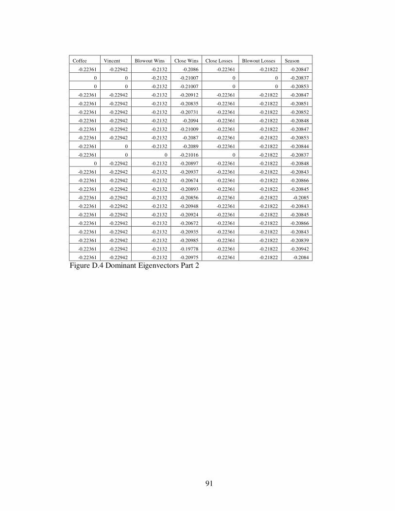
91
Coffee Vincent Blowout Wins Close Wins Close Losses Blowout Losses Season
-0.22361 -0.22942 -0.2132 -0.2086 -0.22361 -0.21822 -0.20847
0 0 -0.2132 -0.21007 0 0 -0.20837
0 0 -0.2132 -0.21007 0 0 -0.20853
-0.22361 -0.22942 -0.2132 -0.20912 -0.22361 -0.21822 -0.20847
-0.22361 -0.22942 -0.2132 -0.20835 -0.22361 -0.21822 -0.20851
-0.22361 -0.22942 -0.2132 -0.20731 -0.22361 -0.21822 -0.20852
-0.22361 -0.22942 -0.2132 -0.2094 -0.22361 -0.21822 -0.20848
-0.22361 -0.22942 -0.2132 -0.21009 -0.22361 -0.21822 -0.20847
-0.22361 -0.22942 -0.2132 -0.2087 -0.22361 -0.21822 -0.20853
-0.22361 0 -0.2132 -0.2089 -0.22361 -0.21822 -0.20844
-0.22361 0 0 -0.21016 0 -0.21822 -0.20837
0 -0.22942 -0.2132 -0.20897 -0.22361 -0.21822 -0.20848
-0.22361 -0.22942 -0.2132 -0.20937 -0.22361 -0.21822 -0.20843
-0.22361 -0.22942 -0.2132 -0.20674 -0.22361 -0.21822 -0.20866
-0.22361 -0.22942 -0.2132 -0.20893 -0.22361 -0.21822 -0.20845
-0.22361 -0.22942 -0.2132 -0.20856 -0.22361 -0.21822 -0.2085
-0.22361 -0.22942 -0.2132 -0.20948 -0.22361 -0.21822 -0.20843
-0.22361 -0.22942 -0.2132 -0.20924 -0.22361 -0.21822 -0.20845
-0.22361 -0.22942 -0.2132 -0.20672 -0.22361 -0.21822 -0.20866
-0.22361 -0.22942 -0.2132 -0.20935 -0.22361 -0.21822 -0.20843
-0.22361 -0.22942 -0.2132 -0.20985 -0.22361 -0.21822 -0.20839
-0.22361 -0.22942 -0.2132 -0.19778 -0.22361 -0.21822 -0.20942
-0.22361 -0.22942 -0.2132 -0.20975 -0.22361 -0.21822 -0.2084
Figure D.4 Dominant Eigenvectors Part 2

92
Colbert
Heights Addison
Cold
Springs Clements Sheffield Tanner Hatton
1st and Long 1 1 0.9711 1 1 1 1
1st and Med 0 0 0.96655 0 0 1 0
1st and Short 0 0 0.96655 1 0 0 0
2nd and Long 1 1 0.96833 1 1 1 1
2nd and Med 1 1 0.97239 1 1 1 1
2nd and Short 1 0 0.9743 1 0 1 1
3rd and Long 1 1 0.97001 1 1 1 1
3rd and Med 1 1 0.96655 1 1 1 1
3rd and Short 1 1 0.96946 1 1 1 1
4th and Long 0 0 0.9698 0 0 1 1
4th and Med 1 0 0 0 0 0 0
4th and Short 1 1 0.97261 1 0 1 1
Left Hash 1 1 0.968 1 1 1 1
Mid. Hash 1 1 0.9756 1 1 1 1
Right Hash 1 1 0.97008 1 1 1 1
Run 1 1 0.97095 1 1 1 1
Pass 1 1 0.96859 1 1 1 1
Left 1 1 0.96886 1 1 1 1
Middle 1 1 0.97574 1 1 1 1
Right 1 1 0.96924 1 1 1 1
Wide 1 1 0.96722 1 1 1 1
Neither 1 1 1 1 1 1 1
Short 1 1 0.96738 1 1 1 1
Figure D.5 Gould Accessibility Indices Part 1

93
Red
Bay Coffee Vincent
Blowout
Wins
Blowout
Losses
Close
Wins
Close
Losses Season
1st and Long 1 1 1 1 1 0.874276 1 0.0996
1st and Med 0 0 0 1 0 0.992803 0 0.0033
1st and Short 0 0 0 1 0 0.992803 0 0.1596
2nd and Long 1 1 1 1 1 0.916108 1 0.0965
2nd and Med 1 1 1 1 1 0.854189 1 0.1389
2nd and Short 1 1 1 1 1 0.770006 1 0.1476
3rd and Long 1 1 1 1 1 0.938812 1 0.1029
3rd and Med 1 1 1 1 1 0.994602 1 0.0962
3rd and Short 1 1 1 1 1 0.88272 1 0.1512
4th and Long 1 1 0 1 1 0.8982 1 0.0668
4th and Med 0 1 0 0 1 1 0 0
4th and Short 1 0 1 1 1 0.903942 1 0.1087
Left Hash 1 1 1 1 1 0.936567 1 0.0575
Mid. Hash 1 1 1 1 1 0.723691 1 0.2738
Right Hash 1 1 1 1 1 0.900592 1 0.076
Run 1 1 1 1 1 0.870914 1 0.1225
Pass 1 1 1 1 1 0.944992 1 0.0561
Left 1 1 1 1 1 0.925717 1 0.0753
Middle 1 1 1 1 1 0.722525 1 0.277
Right 1 1 1 1 1 0.93514 1 0.0625
Wide 1 1 1 1 1 0.975485 1 0.0261
Neither 1 1 1 1 1 0 1 1
Short 1 1 1 1 1 0.967279 1 0.0272
Figure D.6 Gould Accessibility Indices Part 2

94
APPENDIX E
INSTITUTIONAL REVIEW BOARD APPROVAL
Figure E.1 Institutional Review Board Approval Letter