universitat ulm˜
TRANSCRIPT
Universitat Ulm
Institut fur Theoretische Physik
Open Quantum Systems and
Quantum Information Dynamics
Angel Rivas Vargas
Dissertation zur Erlangung des Doktorgrades Dr. rer. nat. der Fakultat furNaturwissenschaften der Universitat Ulm
January 2011
Amtierender Dekan Prof. Dr. Axel Groß
Erstgutachter Prof. Dr. Martin B. Plenio
Zweitgutachter Prof. Dr. Joachim Ankerhold
Tag der Promotion 16. Marz 2011
Dedication
A mis abuelos, Felix, Gertrudis, Carlos y Luisa.
Et si habuero prophetiam,et noverim mysteria omnia, et omnem scientiam,
[. . .] caritatem autem non habuero, nihil sum.1 Cor 13, 2.

Abstract
Just like other theories of physics, quantum theory was developed to explain someexperimental facts that were incomprehensible within the previously existing theo-ries (e.g. the black-body radiation or the photoelectric effect). After the Planck’sintroduction of the concept of quanta at the beginning of the XX century [1], manyphysical situations have been explained by means of quantum mechanics, rangingfrom the behavior of elementary particles to the operational mechanism of stars.Nowadays, about 100 years from its foundation, a lot of effort is being made in try-ing to exploit the genuine features of quantum systems as a resource to solve a widevariety of problems, such as the secure transmission of information, its processingin a more efficient way or to make extremely accurate measurements of physicalquantities.
To carry out this task we require an unprecedented control in the fabricationand manipulation of devices operating in the quantum regime. However, quantumsystems are much more fragile in the presence of noise than their classical coun-terparts, and relevant quantum states allowing novel forms to store, transmit andprocess information vanish very easily. Actually, this is the ultimate reason why wecannot see systems exhibiting quantum behavior in our daily life. As a result, thestudy of the properties of quantum systems in the presence of noise is a fundamentalissue in order to develop any form of reliable quantum technology.
Noise in physical systems can be explained theoretically using the concept of“open system”. Noise arises due to a lack of insulation, in such a way that it is theresult of an effective interaction between our system and its environment. In thisthesis, we present new results concerning the dynamics of open quantum systems.We propose to define rigourously the concept of quantum Markov processes andintroduce quantitative, novel, ways to detect deviations from strict Markovianity.We explore the validity of the usual techniques employed to describe simple openquantum systems, and their extrapolation to more complicated scenarios involvinginteracting and driven systems. In addition we present examples of noise assistedprocesses, and transformations to make these usually tricky problems more efficientlytractable.
In the first part of this thesis we extensively review the general theory of openquantum systems. We introduce new approaches to describe, in a hopefully moretransparent way, some aspects which are usually misleading in a broad range of theliterature. In addition, we revise new concepts and methods developed in recentyears that complement the general theory mainly developed in the 1970s.
In the second part, we focus our attention on the so-called Markovian processeswhich have been described in the previous part. We study the validity of typicalequations used in simple systems such as harmonic oscillators, and propose proposeand check different strategies to describe Markovian dynamics in more complicated
interacting systems. Finally we propose a counterintuitive situation where somelevel of noise can be actually useful for information tasks.
In the third and last part, we approach the problem of the non-Markovian de-scription of open quantum systems. To quantify how non-Markovian an open quan-tum system is we introduce a computable measure and apply it to some relevantsituations. We also propose a way of probing the complexity of an environment byvisualizing properties of a pair of qubits embedded in it. In addition, we developa technique based on orthogonal polynomial theory to transform a wide range ofenvironments into simple chains of particles which can be efficiently simulated withnumerical techniques.
Contents
Acknowledgments 13
1 Introduction 15
I Time Evolution Theory of Open Quantum Systems 19
2 Mathematical tools 212.1 Banach spaces, norms and linear operators . . . . . . . . . . . . . . . 212.2 Exponential of an operator . . . . . . . . . . . . . . . . . . . . . . . . 222.3 Semigroups of operators . . . . . . . . . . . . . . . . . . . . . . . . . 25
2.3.1 Contraction semigroups . . . . . . . . . . . . . . . . . . . . . 272.4 Evolution families . . . . . . . . . . . . . . . . . . . . . . . . . . . . . 30
3 Quantum time evolutions 353.1 Time evolution in closed quantum systems . . . . . . . . . . . . . . . 353.2 Time evolution in open quantum systems. . . . . . . . . . . . . . . . 37
3.2.1 Dynamical maps . . . . . . . . . . . . . . . . . . . . . . . . . 393.2.2 Universal dynamical maps . . . . . . . . . . . . . . . . . . . . 423.2.3 Universal dynamical maps as contractions . . . . . . . . . . . 443.2.4 The inverse of a universal dynamical map . . . . . . . . . . . 463.2.5 Temporal continuity. Markovian evolutions . . . . . . . . . . . 47
3.3 Quantum Markov process: mathematical structure . . . . . . . . . . . 503.3.1 Classical Markovian processes . . . . . . . . . . . . . . . . . . 503.3.2 Quantum Markov evolution as a differential equation . . . . . 513.3.3 Kossakowski conditions . . . . . . . . . . . . . . . . . . . . . . 553.3.4 Steady states of homogeneous Markov processes . . . . . . . . 58
4 Microscopic derivations 654.1 Markovian case . . . . . . . . . . . . . . . . . . . . . . . . . . . . . . 65
4.1.1 Nakajima-Zwanzig equation . . . . . . . . . . . . . . . . . . . 66
7
4.1.2 Weak coupling limit . . . . . . . . . . . . . . . . . . . . . . . 69
4.1.3 Singular coupling limit . . . . . . . . . . . . . . . . . . . . . . 86
4.1.4 Extensions of the weak coupling limit . . . . . . . . . . . . . . 89
4.2 Non-Markovian case . . . . . . . . . . . . . . . . . . . . . . . . . . . 93
4.2.1 Integro-differential models . . . . . . . . . . . . . . . . . . . . 94
4.2.2 Time-convolutionless forms . . . . . . . . . . . . . . . . . . . . 95
4.2.3 Dynamical coarse graining method . . . . . . . . . . . . . . . 97
II Interacting Systems under Markovian Dynamics 101
5 Composite systems of harmonic oscillators 103
5.1 A closer look into the damped harmonic oscillator . . . . . . . . . . . 103
5.1.1 Gaussian states . . . . . . . . . . . . . . . . . . . . . . . . . . 103
5.1.2 Damped harmonic oscillator . . . . . . . . . . . . . . . . . . . 106
5.2 Markovian master equations for interacting systems . . . . . . . . . . 116
5.2.1 Two coupled damped harmonic oscillators . . . . . . . . . . . 117
5.2.2 Driven damped harmonic oscillator . . . . . . . . . . . . . . . 125
5.2.3 Some conclusions . . . . . . . . . . . . . . . . . . . . . . . . . 132
6 Stochastic resonance phenomena in spin chains 135
6.1 Introduction . . . . . . . . . . . . . . . . . . . . . . . . . . . . . . . . 135
6.2 Steady state entanglement in qubit chains subject to longitudinaldecoherence (pure decay) . . . . . . . . . . . . . . . . . . . . . . . . . 136
6.3 XXZ Heisenberg interaction . . . . . . . . . . . . . . . . . . . . . . . 139
6.4 Steady state entanglement under transverse decoherence (pure de-phasing) . . . . . . . . . . . . . . . . . . . . . . . . . . . . . . . . . . 140
6.5 SR phenomena under both longitudinal and transverse decoherence . 142
6.6 Conclusion . . . . . . . . . . . . . . . . . . . . . . . . . . . . . . . . . 144
III Identifying Elements of non-Markovianity 147
7 Measures of non-Markovianity 149
7.1 Introduction . . . . . . . . . . . . . . . . . . . . . . . . . . . . . . . . 149
7.2 Previous attempts . . . . . . . . . . . . . . . . . . . . . . . . . . . . . 149
7.2.1 Proposal of Wolf et. al. . . . . . . . . . . . . . . . . . . . . . . 150
7.2.2 Proposal of Breuer et. al. . . . . . . . . . . . . . . . . . . . . 150
7.2.3 Geometric measures . . . . . . . . . . . . . . . . . . . . . . . 150
7.2.4 Microscopic approach . . . . . . . . . . . . . . . . . . . . . . . 150
7.3 Witnessing non-Markovianity . . . . . . . . . . . . . . . . . . . . . . 151
7.4 Measuring non-Markovianity . . . . . . . . . . . . . . . . . . . . . . . 154
7.5 Conclusions . . . . . . . . . . . . . . . . . . . . . . . . . . . . . . . . 157
8 Probing a composite spin-boson environment 1598.1 Introduction . . . . . . . . . . . . . . . . . . . . . . . . . . . . . . . . 1598.2 System . . . . . . . . . . . . . . . . . . . . . . . . . . . . . . . . . . . 161
8.2.1 Master equation . . . . . . . . . . . . . . . . . . . . . . . . . . 1628.2.2 Observable quantities . . . . . . . . . . . . . . . . . . . . . . . 164
8.3 Results: detecting the presence of coupling between the TLFs . . . . 1648.3.1 Power spectrum of 〈Mx〉 . . . . . . . . . . . . . . . . . . . . . 1658.3.2 Probe entanglement . . . . . . . . . . . . . . . . . . . . . . . . 1678.3.3 Discussion of the results . . . . . . . . . . . . . . . . . . . . . 169
8.4 Decoherence of entangled states . . . . . . . . . . . . . . . . . . . . . 1718.5 Effect of spin-boson environment on entangling gate operations . . . . 1738.6 Some conclusions . . . . . . . . . . . . . . . . . . . . . . . . . . . . . 174
9 Mapping reservoirs to semi-infinite discrete chains 1779.1 Introduction . . . . . . . . . . . . . . . . . . . . . . . . . . . . . . . . 1779.2 Orthogonal polynomials . . . . . . . . . . . . . . . . . . . . . . . . . 179
9.2.1 Basic concepts . . . . . . . . . . . . . . . . . . . . . . . . . . . 1799.2.2 Recurrence relations . . . . . . . . . . . . . . . . . . . . . . . 1809.2.3 Boundness properties of the recurrence coefficients . . . . . . . 182
9.3 System-reservoir structures . . . . . . . . . . . . . . . . . . . . . . . . 1859.4 Applications . . . . . . . . . . . . . . . . . . . . . . . . . . . . . . . . 189
9.4.1 Continuous spin-boson spectral densities . . . . . . . . . . . . 1899.4.2 Discrete spectral densities. The logarithmically discretized
spin-boson model . . . . . . . . . . . . . . . . . . . . . . . . . 1919.4.3 Linearly-discretised baths . . . . . . . . . . . . . . . . . . . . 196
9.5 Conclusions . . . . . . . . . . . . . . . . . . . . . . . . . . . . . . . . 198
Prospects 201
Bibliography 203
Journal Publications
Parts of this thesis are based on material published in the following papers:
• Introduction to the time evolution theory of open quantum systemsA. Rivas and S. F. HuelgaIn preparation(Part I)
• Markovian Master Equations: A Critical StudyA. Rivas, A. D. K. Plato, S. F. Huelga and M. B. PlenioNew J. Phys. 12 113032 (2010)(Chapter 5)
• Exact mapping between system-reservoir quantum models and semi-infinite discrete chains using orthogonal polynomialsA. W. Chin, A. Rivas, S. F. Huelga and M. B. PlenioJ. Math. Phys. 51, 092109 (2010)(Chapter 9).
• Entanglement and non-Markovianity of quantum evolutionsA. Rivas, S. F. Huelga and M. B. PlenioPhys. Rev. Lett. 105, 050403 (2010)(Chapter 7).
• Probing a composite spin-boson environmentN. P. Oxtoby, A. Rivas, S. F. Huelga and R. FazioNew J. Phys. 11, 063028 (2009)(Chapter 8).
• Stochastic resonance phenomena in spin chainsA. Rivas, N. P. Oxtoby and S. F. HuelgaEur. Phys. J. B 69, 51 (2009)(Chapter 6).
Other papers not covered in this thesis to which the author contributed:
• Precision quantum metrology and nonclassicality in linear and non-linear detection schemesA. Rivas and A. LuisPhys. Rev. Lett. 105, 010403 (2010).
10
• Nonclassicality of states and measurements by breaking classicalbounds on statisticsA. Rivas and A. LuisPhys. Rev. A 79, 042105 (2009).
• Practical schemes for the measurement of angular-momentum co-variance matrices in quantum opticsA. Rivas and A. LuisPhys. Rev. A 78, 043814 (2008).
• Intrinsic metrological resolution as a distance measure and nonclas-sical lightA. Rivas and A. LuisPhys. Rev. A 77, 063813 (2008).
• Characterization of angular momentum fluctuations via principalcomponentsA. Rivas and A. LuisPhys. Rev. A 77, 022105 (2008).
11

Acknowledgments
First of all, I wish to express my most heartfelt thanks to my supervisors SusanaHuelga and Martin Plenio. They gave me the opportunity to do research abroad inan extraordinary scientific atmosphere to develop this thesis in the best conditionswhich I could imagine. Their advice and friendship during these years have madethe work of doing a PhD much easier.
It is unavoidable to say many thanks to the people of the Institut fur TheoretischePhysik of the University of Ulm, especially to my corridor-mates Alexandra Liguori,Alex Chin and Ines de Vega, but also to Alex Retzker, Harald Wunderlich, Adolfo delCampo, Marcus Cramer, Javier Prior, Filippo Caruso, Masaki Owari, Shai Machnes,Gor Nikoghosyan, Javier Almeida, Javier Cerrillo-Moreno, Clara Javaherian, MischaWoods, Andreas Albrecht, Tilmann Baumgratz, Robert Rosenbach, Antonio Gentileand particularly to Barbara Bender-Palm (sorry if I forget someone else). I have alsoto give all my thanks to the Herts’ people; Shashank Virmani, Neil Oxtoby, DimitrisTsomokos and Bruce Christianson; and to the Imperial’s guys, Daniel Burgarth,Doug Plato, Fernando Brandao and Animesh Datta.
Furthermore, these years I have met many scientist during visits, meetings andconferences. I got much benefit from discussions with Ramon Aguado, FatithBayazit, Tobias Brandes, Heinz-Peter Breuer, Dariusz Chruscinski, Rosario Fazio,Alberto Galindo, Andrzej Kossakowski, Sabrina Maniscalco, Jyrki Piilo, MiguelAngel Rodriguez, David Salgado, Alessio Serafini, Robert Silbey, Fernando Sols,Herbert Spohn and Michael Wolf.
At this stage, it is impossible to forget my mentors in Complutense Universityof Madrid, Alfredo Luis, Miguel Angel Martın-Delgado and Isabel Gonzalo; thankyou very much for the confidence and support you gave me, I will never forget it.
I would also like to acknowledge the financial and logistic support from theUniversitat Ulm, University of Hertfordshire, the EU projects, CORNER, QAP andQESSENCE.
Of course I am grateful to the members of my examination panel, the chairmanWerner Lutkebohmert, my referees Martin B. Plenio and Joachim Ankerhold, andexaminers Tommaso Calarco and Simone Montangero.
To finalize, let me write in my mother language:
13
La tarea que me propuse de doctorarme en el extranjero hubiera sido imposiblesin el constante apoyo y comprension de mi familia, en especial, de mis padres, JoseMarıa y Marıa Pilar, quienes nunca dejaron que decayera mi animo por poner en talobjetivo lo mejor de mı mismo. Tambien agradezco a mi hermana Pilar por todoslos buenos momentos que hemos pasado juntos, en especial en la etapa de Inglaterra.Del mismo modo, no puedo dejar de agradecer a cada uno de vosotros, tıos, primosy amigos varios que no dejasteis de prestar atencion a lo que hacıa y como andabapor estos “mundos de Dios” con el mejor de los deseos de volver a vernos pronto. Ygracias a quien hace que este trabajo no sea la mayor ilusion de mi vida.
Me gustarıa dedicar esta tesis a mis abuelos, tanto a los que conocı de cerca comoa los que apenas tuve oportunidad de conocer. De ellos y su ejemplo he aprendidotanto que no sabrıa destacar algo, quiza la importancia de formarse tanto academicacomo humanamente para tener mayor oportunidades de vivir con plenitud. Alladonde moreis, y con la esperanza de que el destino nos junte algun dıa, de vuestronieto, Angel.
Laus Deo.
14
Chapter 1
Introduction
This thesis explores the dynamics of open quantum systems, a fundamental, still yetintriguing facets of quantum mechanics. Any real quantum system behaves as anopen quantum system because it is very difficult to find a way to isolate it from itssurroundings. In contrast to classical open systems, it is far more difficult to protecta quantum system from external noise, especially if we wish to control it. Theparadigmatic example is the omnipresence of the quantum vacuum. Although wecan remove all excitations from the surroundings of an atom, the vacuum itself stillposses zero-point energy and, unlike the classical vacuum, dynamical fluctuations.These quantum fluctuations induce processes like spontaneous emission, which arecompletely absent in the classical description of energy dissipation.
Unfortunately, or fortunately, depending on the point of view, all phenomenaarising from quantum coherence are very fragile due to the lack of insulation. Thismakes the implementation of the most fascinating quantum technologies, such asquantum information, quantum computation, or quantum metrology, an extraordi-nary difficult task. However, recent results suggest that a better understanding ofthe dynamics of open quantum systems provides strategies to deal with the presenceof noise in more efficient and promising ways. This is the spirit in which the presentwork has been done.
The necessary background for this thesis is familiarity with the basics of quantummechanics, quantum optics, and quantum information theory.
In Part I a general review of the current theory of open quantum systems ispresented. Despite the existence of very good textbooks on this topic (see for exam-ple [2–15]), they are typically divided into mathematical physics, quantum optics,quantum chemistry and condensed matter, which have very different approaches tothe problem. This part of the thesis gives a unified description of the open systemdynamics which takes into account new concepts and explains carefully the smallsubtleties usually omitted in the literature of open quantum systems. It consists ofchapters 2, 3, and 4.
Chapter 2 presents the mathematical formalism used throughout this thesis.Some fundamental properties of Banach spaces are explained, like norm, spec-
15
trum and resolvent of linear operators. Next the exponential operator is de-fined and some of its properties are analyzed; this will lead us to the intro-duction of the concept of the one-parameter semigroup. In particular, theso-called contraction semigroups will be carefully explained and the main the-orems about them (in finite dimensions) presented. Finally, the evolutionfamilies, which are more general structures which appear in the analysis ofnon-autonomous differential problems, will also be briefly reviewed.
Chapter 3 gives a brief recapitulation of the main features of the dynamics ofclosed quantum systems. These are described by the Schrodinger equationand unitary evolutions. These concepts will be the starting point for theanalysis of more general dynamics. Then an overview of the dynamics ofopen quantum systems is presented. The view of an open quantum systemas a part of a larger closed systems leads to the concept of partial trace anddynamical maps. Determining the circumstances under which an induceddynamical map is universal, i.e. it transforms any quantum state in anothervalid quantum state is an important problem which has not received muchattention in the literature. Here this issue will be discussed in detail, andthe universal dynamical maps will be introduced in an alternative way. Inaddition we explain some important properties of the universal dynamics asthey provide us with a physical definition of Markovianity in the quantum case.This concept will be fundamental in the rest of the thesis. Next, it is explainedhow, apart of a physical point of view, there is an analogy of the concept ofquantum Markovianity with the classical Markovianity, and enumerates someof the most important mathematical properties. On one hand, a simplifiedproof is presented which shows that an evolution is Markovian if and only ifit can be written as a time dependent Kossakowski-Lindblad master equation.Details of the traditional derivation of the homogeneous case by Kossakowskiare also given. On the other hand we provide a brief introduction to therelaxing properties of homogeneous Markovian dynamics.
Chapter 4 deals with the way to the evolution of an open quantum system froma microscopic point of view, i.e. starting from a Hamitonian for the wholeclosed system and tracing out the environmental degrees of freedom. Werecall that a Markovian model is a good approximation of the real dynamicsin two limits, namely, the weak coupling and the singular coupling limit. Bothof these are explained, but we pay special attention to the weak coupling limitbecause it is used the most in practical situations. Furthermore we avoidsome arguments which are usually given to justify this limit, showing thatthey can be misleading. In addition, the extension of the weak coupling limitto situations with interacting systems is partially described. Finally it is alsoprovided an introduction to non-Markovian dynamics from a microscopic pointof view. Some integro-differential models and the time-convolutionless formsare presented. Furthermore we also explain the so-called dynamical coarsegraining method.
16
After the general introduction to open quantum systems in Part I, we analyzenew results concerning Markovian dynamics in Part II of the thesis. It consist ofchapters 5 and 6.
Chapter 5 has two main objectives. The first is to introduce how to do an exactnumerical simulation of a set of coupled harmonic oscillators by using Gaus-sian states. The second aim is to make a thorough study of the dynamics ofdamped harmonic oscillators. We check the limits where the exact dynamicsbecomes Markovian, finding that the Markovian master equation is quite agood description even for regimes where the literature claims that the Marko-vian approximation fails, e.g. at low temperatures. Furthermore we extendthe analysis for the case of interacting systems. We derive Markovian mas-ter equations for interacting harmonic systems in different scenarios, includingstrong internal coupling and classically driven. By comparing the dynamics re-sulting from the corresponding master equations with numerical simulations ofthe global system’s evolution, we determine the regimes where the Markovianapproximation is valid, and assess the robustness of the assumptions made inthe process of deriving the reduced Markovian dynamics.
Chapter 6 changes the topic slightly. We analyze the steady state behavior quan-tum correlations (entanglement) as well as the global correlations in the systemwhen subject to different forms of local Markovian decoherence. In the pres-ence of decay, it has been shown that the system displays quantum correlationsonly when the noise strength is above a certain threshold. We extend this re-sult to the case of a Heisenberg XXZ interaction and revise and clarify themechanisms underlying this behavior. In the presence of pure dephasing, weshow that the system always remains separable in the steady state. Whenboth types of noise are present, the system can still exhibit entanglement forlong times, provided that the pure dephasing rate is not too large.
As we explain during Part I of the thesis, the study of non-Markovian dynam-ics is more complicated than the Markovian case. However no real dynamics areexactly Markovian and experimental data from solid-state devices or soft-mattersystems strongly suggest that the non-Markovian properties of the dynamics arevery important. Therefore new results in the field of non-Markovian dynamics areattaching increasing attention. Part III of this thesis concerns new methods relatedto the description of non-Markovian systems and consists of chapters 7, 8 and 9.
Chapter 7 the problem of quantifying the non-Markovian character of quantumtime evolutions of general systems in contact with an environment is addressed.We introduce two different measures of non-Markovianity that exploit the spe-cific traits of quantum correlations and which are suitable for opposite experi-mental contexts. When complete tomographic knowledge about the evolutionis available, our measure lies in a necessary and sufficient condition to quan-tify strictly the non-Markovianity. In the opposite case, when no information
17
whatsoever is available, we propose a sufficient condition for non-Markovianity.Remarkably, no optimization procedure underlies our derivation, which greatlyenhances the practical relevance of the proposed criteria.
Chapter 8 deals with the problem of environmental characterization. We considernon-interacting multi-qubit systems as controllable probes of an environmentof defects/impurities modeled as a composite spin-boson environment. Thiscomposite spin-boson environment consists of a small number of quantum-coherent two-level fluctuators damped by independent bosonic baths. We dis-cuss how correlation measurements in the probe system encode informationabout the environment structure, and how they could be exploited to dis-criminate efficiently between different experimental preparation techniques.Particular attention is given to the quantum correlations (entanglement) thatbuild up in the probe as a result of the environment-mediated interaction.We also investigate the harmful effects of the composite spin-boson environ-ment on initially prepared entangled bipartite qubit states of the probe andon entangling gate operations. Our results offer insights in the area of quan-tum computation using superconducting devices, where defects/impurities arebelieved to be a major source of decoherence.
Chapter 9 presents an exact unitary transformation that maps the Hamiltonianof a quantum system coupled linearly to a continuum of bosonic or fermionicmodes to a Hamiltonian that describes a one-dimensional chain with onlynearest-neighbor interactions, which can be efficiently simulated. The keypoint is the use of the properties of orthogonal polynomials. This analyticaltransformation predicts a simple set of relations between the parameters ofthe chain and the recurrence coefficients of the orthogonal polynomials usedin the transformation and allows the chain parameters to be computed usingnumerically stable algorithms that have been developed to compute recur-rence coefficients. We then prove some general properties of this chain systemfor a wide range of spectral functions and give examples drawn from physi-cal systems where exact analytic expressions for the chain properties can beobtained.
Finally, in the section on prospects, we suggest potential applications of the ideasand methods contained in this thesis. We also give in advance partial results whichare being prepared for publication, and furthermore we discuss several unansweredquestions about the dynamics of open quantum system for which the aforementionedmethods may be applied.
18
Part I
Time Evolution Theory of OpenQuantum Systems
19

Chapter 2
Mathematical tools
2.1 Banach spaces, norms and linear operators
In different parts within this work, we will make use of properties of Banach spaces.For our interest it is sufficient to restrict our analysis to finite dimensional spaces.In what follows we revise some basic concepts [16–18].
2.1.1. Definition. A Banach space B is a complete linear space with a norm ‖ ·‖.
Recall that an space is complete if every Cauchy sequence converges in it. Anexample of Banach space is provided by the set of self-adjoint trace-class linearoperators over a Hilbert space H. This is, the self-adjoint operators whose tracenorm is finite ‖ · ‖1
‖A‖1 = Tr√
A†A = Tr√
A2, A ∈ B.
Now we focus our attention onto possible linear transformations over a Banachspace, that we will denote by T (B) : B 7→ B. The set of all of them form the dualspace B∗.
2.1.2. Proposition. The dual space of B, B∗ is a (finite) Banach space with theinduced norm
‖T‖ = supx∈B,x 6=0
‖T (x)‖‖x‖ = sup
x∈B,‖x‖=1
‖T (x)‖, T ∈ B∗.
Proof : The proof is basic.Apart from the triangle inequality, the induced norm fulfills some other useful
inequalities. For example, immediately from the definition one obtains that
‖T (x)‖ ≤ ‖T‖‖x‖, ∀x ∈ B. (2.1)
Moreover,
21
2.1.3. Proposition. Let T1 and T2 be two linear operators in B∗, then
‖T1T2‖ ≤ ‖T1‖‖T2‖ (2.2)
Proof. This is just a consequence of the inequality (2.1); indeed,
‖T1T2‖ = supx∈B,‖x‖=1
‖T1T2(x)‖ ≤ supx∈B,‖x‖=1
‖T1‖‖T2(x)‖ = ‖T1‖‖T2‖.
2
The next concept will appear quite often in the coming sections.
2.1.4. Definition. A linear operator T over a Banach space B, is said to be acontraction if
‖T (x)‖ ≤ ‖x‖, ∀x ∈ B,
this is ‖T‖ ≤ 1.
Finally, we briefly revise some additional basic concepts that will be featured insubsequent sections.
2.1.5. Definition. For any linear operator T in a (finite) Banach space B, itsresolvent operator is defined as
RT (λ) = (λ1− T )−1, λ ∈ C.
It is said that λ ∈ C belongs to the (point) spectrum of T , λ ∈ σ(T ), if RT (λ) doesnot exist; otherwise λ ∈ C belongs to the resolvent set of T , λ ∈ %(T ). As a resultσ(T ) and %(T ) are said to be complementary sets.
The numbers λ ∈ σ(T ) are called eigenvalues of T , and each element in thekernel x ∈ ker(λ1 − T ), which is obviously different from 0 as (λ1 − T )−1 doesnot exist, will be called the eigenvector associated with the eigenvalue λ.
2.2 Exponential of an operator
The operation of exponentiation of an operator is of special importance in relationwith linear differential equations.
2.2.1. Definition. The exponential of a linear operator L in a finite Banach spaceis defined as
eL =∞∑
n=0
Ln
n!. (2.3)
The following proposition shows that this definition is indeed meaningful.
2.2.2. Proposition. The series defining eL is absolutely convergent.
22
Proof. The following chain of inequalities holds
‖eL‖ =
∥∥∥∥∥∞∑
n=0
Ln
n!
∥∥∥∥∥ ≤∞∑
n=0
‖Ln‖n!
≤∞∑
n=0
‖L‖n
n!= e‖L‖.
Since e‖L‖ is a numerical series which is convergent, the norm of eL is upper boundedand therefore the series converges absolutely.
2
2.2.3. Proposition. If L1 and L2 commute with each other, then e(L1+L2) = eL1eL2 =eL2eL1.
Proof. By using the binomial formula as in the case of a numerical series, weobtain
e(L1+L2) =∞∑
n=0
(L1 + L2)n
n!=
∞∑n=0
1
n!
n∑
k=0
(n
k
)Lk
1Ln−k2
=∞∑
n=0
n∑
k=0
1
k!(n− k)!Lk
1Ln−k2 =
∞∑p=0
∞∑q=0
1
p!q!Lp
1Lq2 = eL1eL2 = eL2eL1 .
2
The above result does not hold when L1 and L2 are not commuting operators,in that case there is a formula which is sometimes useful.
2.2.4. Theorem (Lie-Trotter product formula). Let L1 and L2 be linearoperators in a finite Banach space, then:
e(L1+L2) = limn→∞
(e
L1n e
L2n
)n
Proof. We present a two-step proof inspired by [19]. First let us prove that forany two linear operators A and B the following identity holds:
An −Bn =n−1∑
k=0
Ak(A−B)Bn−k−1. (2.4)
We observe that, at the end, we are only adding and subtracting the products ofpowers of A and B in the right hand side of (2.4), so that
An −Bn = An + (An−1B − An−1B)−Bn
= An + (An−1B − An−1B + An−2B2 − An−2B2)−Bn =
= An + (An−1B − An−1B + An−2B2 − An−2B2 + . . .
· · ·+ ABn−1 − ABn−1)−Bn.
23
Now we can add terms with positive sign to find:
An + An−1B + . . . + ABn−1 =n−1∑
k=0
Ak+1Bn−k−1,
and all terms with negative sign to obtain:
−An−1B − . . .− ABn−1 −Bn = −n−1∑
k=0
AkBn−k.
Finally, by adding both contributions one gets that
An −Bn =n−1∑
k=0
Ak+1Bn−k−1 − AkBn−k =n−1∑
k=0
Ak(A−B)Bn−k−1,
as we wanted to prove.Now, we name
Xn = e(L1+L2)/n, Yn = eL1/neL2/n,
and take A = Xn and B = Yn in formula (2.4),
Xnn − Y n
n =n−1∑
k=0
Xkn(Xn − Yn)Y n−k−1
n .
On the one hand,
‖Xkn‖ = ‖ (
e(L1+L2)/n)k ‖ ≤ ‖e(L1+L2)/n‖k ≤ e‖L1+L2‖k/n
≤ e(‖L1‖+‖L2‖)k/n ≤ e‖L1‖+‖L2‖, ∀k ≤ n.
Similarly, one proves that
‖Y kn ‖ ≤ e‖L1‖+‖L2‖, ∀k ≤ n.
So we get
‖Xnn − Y n
n ‖ ≤n−1∑
k=0
‖Xkn(Xn − Yn)Y n−k−1
n ‖ ≤n−1∑
k=0
‖Xkn‖‖Xn − Yn‖‖Y n−k−1
n ‖
≤n−1∑
k=0
‖Xn − Yn‖e2(‖L1‖+‖L2‖) = n‖Xn − Yn‖e2(‖L1‖+‖L2‖).
On the other hand, by expanding the exponential we find that
limn→∞
n‖Xn − Yn‖ = limn→∞
n
∥∥∥∥∥∞∑
k=0
1
k!
(L1 + L2
n
)k
−∞∑
k,j=0
1
k!j!
(L1
n
)k (L2
n
)j∥∥∥∥∥
≤ limn→∞
n
∥∥∥∥1
2n2[L2, L1] +O
(1
n3
)∥∥∥∥ = 0.
24
Therefore we finally arrive at the result that:
limn→∞
∥∥∥eL1+L2 − (eL1/neL2/n
)n∥∥∥ = lim
n→∞‖Xn
n − Y nn ‖ = 0.
2
Using a similar procedure one can also show that for a sum of N general operators,the following identity holds:
e∑N
k=1 Lk = limn→∞
(N∏
k=1
eLkn
)n
. (2.5)
2.3 Semigroups of operators
2.3.1. Definition. [Semigroup] A family of linear operators Tt (t ≥ 0) on a finiteBanach Space forms a one-parameter semigroup if
1. TtTs = Tt+s, ∀t, s2. T0 = 1.
2.3.2. Definition. [Uniformly Continuous Semigroup] A one-parameter semigroupTt is said to be uniformly continuous if the map
t 7→ Tt
is continuous, this is, if lima→b ‖Ta − Tb‖ = 0. This kind of continuity is normallyreferred to as “continuity in the uniform operator topology” [16], and it is sufficientto analyze the finite dimensional case, which is the focus of this work.
2.3.3. Theorem. If Tt forms a uniformly continuous one-parameter semigroup,then the map t 7→ Tt is differentiable, and the derivative of Tt is given by
dTt
dt= LTt,
with L = dTt
dt|t=0.
Proof. Since Tt is uniformly continuous on t, the function V (t) defined by
V (t) =
∫ t
0
Tsds, t ≥ 0,
is differentiable with dV (t)dt
= Tt (to justify this it is enough to consider the well-known arguments used for the case of R, see for example [20], but substituting nowthe absolute value by the concept of norm). In particular,
limt→0
V (t)
t= lim
t→0
V (t)− V (0)
t=
dV (t)
dt
∣∣∣∣t=0
= T0 = 1,
25
this implies that there exist some t0 > 0 small enough such that V (t0) is invertible.Then,
Tt = V −1(t0)V (t0)Tt = V −1(t0)
∫ t0
0
TsTtds = V −1(t0)
∫ t0
0
Tt+sds
= V −1(t0)
∫ t+t0
t
Tsds = V −1(t0) [V (t + t0)− V (t)] ,
since the difference of differentiable functions is differentiable, Tt is differentiable.Moreover, its derivative is
dTt
dt= lim
h→0
Tt+h − Tt
h= lim
h→0
Th − 1h
Tt = LTt.
2
2.3.4. Theorem. The exponential operator T (t) = eLt is the only solution of thedifferential problem
dT (t)dt
= LT (t), t ∈ R+
T (0) = 1,
Proof. From the definition of exponential given by Eq. (2.3), it is clear thatT (0) = 1, and because of the commutativity of the exponents we find
deLt
dt= lim
h→0
eL(t+h) − eLt
h=
(limh→0
eLh − 1h
)eLt.
By expanding the exponential one obtains
limh→0
eLh − 1h
= limh→0
1+ Lh +O(h2)− 1h
= L.
At this point, it just remains to prove uniqueness. Let us consider another functionS(t) and assume that it also satisfies the differential problem. Then we define
Q(s) = T (s)S(t− s), for t ≥ s ≥ 0,
for some fixed t > 0, so Q(s) is differentiable with derivative
dQ(s)
ds= LT (s)S(t− s)− T (t)LS(t− s) = LT (s)S(t− s)− LT (t)S(t− s) = 0.
Q(s) is therefore a constant function. In particular Q(s) = Q(0) for any t ≥ s ≥ 0,which implies that
T (t) = T (t)S(t− t) = Q(t) = Q(0) = S(t).
2
26
2.3.1. Collolary. Any uniformly continuous semigroup can be written in the formTt = T (t) = eLt, where L is called the generator of the semigroup and it is the onlysolution to the differential problem
dTt
dt= LTt, t ∈ R+
T0 = 1.(2.6)
Given the omnipresence of differential equations describing time-evolution inphysics, it is now evident why semigroups are important. If we can extend thedomain of t to negative values, then Tt forms a one-parameter group whose inversesare given by T−t, so that TtT−t = 1 for all t ∈ R.
There is a special class of semigroups which is important for our proposes, andthat will be the subject of the next section.
2.3.1 Contraction semigroups
2.3.5. Definition. A one-parameter semigroup satisfying ‖Tt‖ ≤ 1 for every t ≥ 0,is called a contraction semigroup.
Now one question arises, namely, which properties does the generator L have tofulfill to generate a contraction semigroup? This is an intricate question in generalthat is treated with more detail in functional analysis textbooks such as [21–23]. Forfinite dimensional Banach spaces, the proofs of the main theorems can be drasticallysimplified, and they are presented in the following. The main condition are basedin properties of the resolvent set and the resolvent operator.
2.3.6. Theorem (Hille-Yoshida). A necessary and sufficient condition for alinear operator L to generate a contraction semigroup is that
1. λ, Re λ > 0 ⊂ %(L).
2. ‖RL(λ)‖ ≤ (Re λ)−1.
Proof. Let L be the generator of a contraction semigroup and λ a complex number.For a ≥ b we define the operator
L(a, b) =
∫ b
a
e(−λ1+L)tdt.
Since the exponential series converges uniformly (to see this one uses again tools ofthe elementary analysis, specifically the M-test of Weierstrass [20], over the Banachspace B) it is possible to integrate term by term in the previous definition
L(a, b) =
∫ b
a
∞∑n=0
(−λ1+ L)ntn
n!dt =
∞∑n=0
(−λ1+ L)n
n!
(∫ b
a
tndt
)
=∞∑
n=0
(−λ1+ L)n
n!
[bn+1
n + 1− an+1
n + 1
].
27
Thus by multiplying L(a, b) by (λ1− L) we get
(λ1− L)L(a, b) = L(a, b)(λ1− L) =[e(−λ1+L)a − e(−λ1+L)b
].
Now assume Re λ > 0 and take the limit a → 0, b →∞, then as
limb→∞
‖e(−λ1+L)b‖ = limb→∞
‖e−λ1beLb‖ ≤ limb→∞
‖e−λ1b‖‖eLb‖≤ lim
b→∞‖e−λ1b‖ = 0,
andlima→0
e−λ1aeLa = 1,
we get
(λ1− L)
[∫ ∞
0
e−λ1teLtdt
]=
[∫ ∞
0
e−λ1teLtdt
](λ1− L) = 1.
So if Reλ > 0 then λ ∈ %(L) and from the definition of the resolvent operator weget
RL(λ) =
∫ ∞
0
e−λ1teLtdt.
Moreover,
‖RL(λ)‖ =
∥∥∥∥∫ ∞
0
e−λ1teLtdt
∥∥∥∥ ≤∫ ∞
0
‖e−λ1teLt‖dt ≤∫ ∞
0
‖e−λ1t‖‖eLt‖dt
≤∫ ∞
0
‖e−λ1t‖dt =
∫ ∞
0
|e−λt|dt =
∫ ∞
0
e−Re(λ)tdt =1
Re(λ).
Conversely, suppose that L satisfies the above conditions 1 and 2. Let λ be somereal number in the resolvent set of L, which means it is also a real positive number.We define the operator
Lλ = λLRL(λ),
it turns out that Lλ → L as λ →∞. Indeed, it is enough to show that λRL(λ) → 1.Since (0,∞) ⊂ %(L) there is no problem with the resolvent operator taking the limit,so by writing λRL(λ) = LRL(λ) + 1 we obtain
limλ→∞
‖λRL(λ)− 1‖ = limλ→∞
‖LRL(λ)‖ ≤ limλ→∞
‖L‖‖RL(λ)‖ ≤ limλ→∞
‖L‖λ
= 0,
where we have used 2. Moreover,
‖eLλt‖ = ‖eλLRL(λ)t‖ = ‖e[λ2RL(λ)−λ1]t‖ ≤ e−λt‖eλ2RL(λ)t‖≤ e−λteλ2‖RL(λ)‖t ≤ e−λteλt = 1,
and thereforeeLt = lim
λ→∞eLλt
28
is a contraction semigroup.2
Apart from imposing conditions such that L generates a contraction semigroup,this theorem is of vital importance in general operator theory over arbitrary dimen-sional Banach spaces. If the conditions of the theorem 2.3.6 are fulfilled then Lgenerates a well-defined semigroup; note that for general operators L the exponen-tial cannot be rigourously defined as a power series, and more complicated tools areneeded. On the other hand, to apply this theorem directly can be complicated inmany cases, so one needs more manageable equivalent conditions.
2.3.7. Definition. A semi-inner product is an operation in which for each pairx1, x2 of elements of a Banach space B there is a complex number [x1, x2] associatedwith it such that
[x1, λx2 + µx3] = λ[x1, x2] + µ[x1, x3], (2.7)
[x1, x1] = ‖x1‖2 (2.8)
|[x1, x2]| ≤ ‖x1‖‖x2‖. (2.9)
for any x1, x2, x3 ∈ B and λ, µ ∈ C.
2.3.8. Definition. A linear operator L in B is called dissipative if
Re[x, Lx] ≤ 0 ∀x ∈ B. (2.10)
2.3.9. Theorem (Lumer-Phillips). A necessary and sufficient condition for alinear operator L in B (of finite dimension) to be the generator of a contractionsemigroup is that L be dissipative.
Proof. Suppose that Tt, t ≥ 0 is a contraction semigroup, then just by usingthe properties of a semi-inner product we have that:
Re[x, (Tt − 1)x] = Re[x, Ttx]− ‖x‖2 ≤ |[x, Ttx]| − ‖x‖2
≤ ‖x‖‖Ttx‖ − ‖x‖2 ≤ ‖x‖2‖Tt‖ − ‖x‖2 ≤ 0
since ‖Tt‖ ≤ 1. So L is dissipative
Re[x, Lx] = limt→0
1
tRe[x, (Tt − 1)x] ≤ 0.
Conversely, let L be dissipative. Considering a point within its spectrum λ ∈ σ(L)and a corresponding eigenvector x ∈ ker(λ1− L), since [x, (λ1− L)x] = 0 we have
Re[x, (λ1− L)x] = Re(λ)‖x‖2 − Re[x, Lx] = 0,
29
given that Re[x, Lx] ≤ 0, Re(λ) ≤ 0. Thus any complex number Re(λ) > 0 is inthe resolvent of L. Moreover, let λ ∈ %(L), we have again from the properties of asemi-inner product that
Re(λ)‖x‖2 = Re(λ)[x, x] ≤ Re(λ[x, x]− [x, Lx]) = Re[x, (λ1− L)x]
≤ |[x, (λ1− L)x]| ≤ ‖x‖‖(λ1− L)x‖so ‖(λ1 − L)x‖ ≥ Re(λ)‖x‖, ∀x 6= 0. Then, by setting x = (λ1 − L)x in theexpression for the norm of RL(λ) we can write that
‖RL(λ)‖ = supx∈B,x 6=0
‖RL(λ)x‖‖x‖ = sup
x∈B,x/∈ker(λ1−L)
‖x‖‖(λ1− L)x‖
≤ ‖x‖Re(λ)‖x‖ =
1
Re(λ),
and therefore L satisfies the conditions of the theorem 2.3.6.2
2.4 Evolution families
As we have seen semigroups arise naturally in the context of problems involving lin-ear differential equations, as exemplified by Eq. (2.6), with time-independent gen-erators L. However some situations in physics require solving time-inhomogeneousdifferential problems,
dxdt
= L(t)x, x ∈ B
x(t0) = x0,
where L(t) is a time-dependent linear operator. Given that the differential equationis linear, its solution must depend linearly on the initial conditions, so we can write
x(t) = T(t,t0)x(t0), (2.11)
where T(t,t0) is a linear operator often referred to as the evolution operator. Obvi-ously, T(t0,t0) = 1 and the composition of two consecutive evolution operators is welldefined, since for t2 ≥ t1 ≥ t0
x(t1) = T(t1,t0)x(t0) and x(t2) = T(t2,t1)x(t1).
As a result, the evolution operator between t2 and t0 is given by
T(t2,t0) = T(t2,t1)T(t1,t0), (2.12)
and the two-parameter family of operators T (t, s) fulfills the properties
T(t,s) = T(t,r)T(r,s), t ≥ r ≥ sT(s,s) = 1.
(2.13)
30
These operators are sometimes called evolution families, propagators, or funda-mental solutions. One important fact to realize is that if the generator is time-independent, L, the evolution family is reduced to a one-parameter semigroup intime difference T(t,s) = Tτ=t−s. However, in contrast to general semigroups, it is notenough (even in finite dimension) to require that the map (t, s) 7→ T(t,s) be contin-uous to ensure that it is differentiable [24], although in practice we usually assumethat the temporal evolution is smooth enough and families fulfilling Eq. (2.13) willalso considered to be differentiable. Under these conditions we can formulate thefollowing result.
2.4.1. Theorem. A differentiable family T(t,s) obeying the condition (2.13) is theonly solution to the differential problems
dT(t,s)
dt= L(t)T(t,s), t ≥ s
T(s,s) = 1,
and dT(t,s)
ds= −T(t,s)L(t), t ≥ s
T(s,s) = 1.
Proof. If the evolution family T(t,s) is differentiable
dT(t,s)
dt= lim
h→0
T(t+h,s) − T(t,s)
h= lim
h→0
T(t+h,t) − 1h
T(t,s) = L(t)T(t,s).
Analogously one proves that
dT(t,s)
ds= −T(t,s)L(t).
To show that this solution is unique, as in theorem 2.3.4, let us assume that thereexist some other S(t,s) solving the differential problems. Then, for every fixed t ands, we define now Q(r) = T(t,r)S(r,s) for t ≥ r ≥ s. It is immediate to show thatdQ(r)
dr= 0 and therefore
T(t,s) = Q(s) = Q(t) = S(t,s).
2
Again opposed to the case of semigroups, to give a general expression for anevolution family T(t,s) in terms of the generator L(t) is complicated. To illustratewhy let us define first the concept of time-ordering operator.
2.4.2. Definition. The time-ordered operator T of a product of two operatorsL(t1)L(t2) is defined by
T L(t1)L(t2) = θ(t1 − t2)L(t1)L(t2) + θ(t2 − t1)L(t2)L(t1),
31
where θ(x) is the Heaviside step function. Similarly, for a product of three operatorsL(t1)L(t2)L(t3), we have
T L(t1)L(t2)L(t3) = θ(t1 − t2)θ(t2 − t3)L(t1)L(t2)L(t3)
+ θ(t1 − t3)θ(t3 − t2)L(t1)L(t3)L(t2)
+ θ(t2 − t1)θ(t1 − t3)L(t2)L(t1)L(t3)
+ θ(t2 − t3)θ(t3 − t1)L(t2)L(t3)L(t1)
+ θ(t3 − t1)θ(t1 − t2)L(t3)L(t1)L(t2)
+ θ(t3 − t2)θ(t2 − t1)L(t3)L(t2)L(t1)
so that for a product of k operators L(t1) · · ·L(tk) we can write:
T L(t1) · · ·L(tk) =∑
π
θ[tπ(1) − tπ(2)] · · · θ[tπ(k−1) − tπ(k)]L[tπ(1)] · · ·L[tπ(k)] (2.14)
where π is a permutation of k indexes and the sum extends over all k! differentpermutations.
2.4.3. Theorem (Dyson Series). Let be the generator L(t′) bounded in the in-terval [t, s], i.e. ‖L(t′)‖ < ∞, t′ ∈ [t, s]. Then the evolution family T(t,s) admits thefollowing series representation
T (t, s) = 1+∞∑
m=1
∫ t
s
∫ t1
s
· · ·∫ tm−1
s
L(t1) · · ·L(tm)dtm · · · dt1, (2.15)
where t ≥ t1 ≥ . . . ≥ tm ≥ s, and it can be written symbolically as
T (t, s) = T e∫ t
s L(t′)dt′ ≡ 1+∞∑
m=1
1
m!
∫ t
s
· · ·∫ t
s
T L(t1) · · ·L(tm)dt1 · · · dtm (2.16)
Proof. To prove that expression (2.15) can be formally written as (2.16) note thatby introducing the time-ordering definition Eq. (2.14), the kth term of this seriescan be written as
1
k!
∫ t
s
· · ·∫ t
s
T L(t1) · · ·L(tk)dt1 · · · dtk
=1
k!
∑π
∫ t
s
∫ tπ(1)
s
· · ·∫ tπ(k−1)
s
L[tπ(1)] · · ·L[tπ(k)]dt1 · · · dtk
=
∫ t
s
∫ t1
s
· · ·∫ tk−1
s
L(t1) · · ·L(tk)dtk · · · dt1,
where in the last step we have used that t ≥ tπ(1) ≥ . . . ≥ tπ(k) ≥ s, and that thename of the variables does not matter, so the sum over π is the addition of the sameintegral k! times.
32
To prove Eq. (2.15), we need first of all to show that the series is convergent,but this is simple because by taking norms in (2.16) we get the upper bound
‖T (t, s)‖ ≤∞∑
m=0
|t− s|mm!
(sup
t′∈[s,t]
‖L(t′)‖)m
= exp
[sup
t′∈[s,t]
‖L(t′)‖|t− s|]
which is convergent as a result of L(t′) being bounded in [t, s]. Finally, the fact that(2.15) is the solution of the differential problem is easy to verify by differentiatingthe series term by term since it converges uniformly and so does its derivative (tosee this one use again the M-test of Weierstrass [20] over the Banach space B). 2
This result is the well-known Dyson expansion, which is widely used for instancein scattering theory. We have proved its convergence for finite dimensional systemsand bounded generator. This is normally difficult to prove in the infinite dimensionalcase, but the expression is still used in this context in a formal sense.
Apart from the Dyson expansion, there is an approximation formula for evolutionfamilies which will be useful in this work.
2.4.4. Theorem (Time-Splitting formula). The evolution family T(t,s) can begiven by the formula
T(t,s) = limmax |tj+1−tj |→0
0∏j=n−1
e(tj+1−tj)L(tj) for t = tn ≥ . . . ≥ t0 = s, (2.17)
where L(tj) is the generator evaluated in the instantaneous time tj (note the de-scending order in the product symbol).
Proof. The idea for this proof is taken from [25], more rigorous and general proofscan be found in [21, 22]. Given that the product in (2.17) is already temporallyordered, nothing happens if we introduce the temporal-ordering operator
T(t,s) = limmax |tj+1−tj |→0
T0∏
j=n−1
e(tj+1−tj)L(tj),
= limmax |tj+1−tj |→0
T e∑n−1
j=0 (tj+1−tj)L(tj),
where one realizes that the time ordering operator is then making the work ofordering the terms in the exponential series on the bottom term in order to obtainthe same series expansion as on the top term. Now it only remains to recognize theRiemann sum [20] in the exponent to arrive at the expression
T(t,s) = T e∫ t
s L(t′)dt′ ,
which is Eq. (2.16). 2
In analogy to the case of contraction semigroups, one can define contractionevolution families. However, since we now have two parameters, there is not aunique possible definition, as illustrated below.
33
2.4.5. Definition. An evolution family T(t,s) is called contractive if ‖T(t,s)‖ ≤ 1for every t and every s such that t ≥ s.
2.4.6. Definition. An evolution family T(t,s) is called eventually contractive ifthere exist a s0 such that ‖T(t,s0)‖ ≤ 1 for every t ≥ s0.
It is clear that contractive families are also eventually contractive, but in thissecond case there exist a privileged initial time s0, such that one can have ‖T(t,s)‖ > 1for some s 6= s0. This distinction is relevant and will allow us later on to discriminateuniversal dynamical maps given by differential equations which are Markovian fromthose which are not.
34
Chapter 3
Quantum time evolutions
3.1 Time evolution in closed quantum systems
Probably time evolution of physical systems is the main factor in order to understandtheir nature and properties. In classical systems time evolution is usually formu-lated in terms of differential equations (i.e. Euler-Lagrange’s equations, Hamilton’sequations, Liouville equation, etc.), which can present very different characteristicsdepending on which physical system they correspond to. From the beginning of thequantum theory, physicists have been often trying to translate the methods whichwere useful in the classical case to the quantum one, so was that Erwin Schrodingerobtained the first evolution equation for a quantum system in 1926 [26].
This equation, called Schrodinger’s equation since then, describes the behaviorof an isolated or closed quantum system, that is, by definition, a system which doesnot interchanges information (i.e. energy and/or matter [27]) with another system.So if our isolated system is in some pure state |ψ(t)〉 ∈ H at time t, where Hdenotes the Hilbert space of the system, the time-evolution of this state (betweentwo consecutive measurements) is according to
d
dt|ψ(t)〉 = − i
~H(t)|ψ(t)〉, (3.1)
where H(t) is the Hamiltonian operator of the system. In the case of mixed statesρ(t) the last equation naturally induces
dρ(t)
dt= − i
~[H(t), ρ(t)], (3.2)
sometimes called von Neumann or Liouville-von Neumann equation, mainly in thecontext of statistical physics. From now on we consider units where ~ = 1.
There are several ways to justify the Schrodinger equation, some of them relatedwith heuristic approaches or variational principles, however in all of them it is nec-essary to make some extra assumptions apart from the postulates about states andobservables; for that reason the Schrodinger equation can be taken as another postu-late. Of course the ultimate reason for its validity is that the experimental tests are
35
in accordance with it [28–30]. In that sense, the Schrodinger equation is for quantummechanics as fundamental as the Maxwell’s equations for electromagnetism or theNewton’s Laws for classical mechanics.
An important property of Schrodinger equation is that it does not change thenorm of the states, indeed
d
dt〈ψ(t)|ψ(t)〉 =
(d〈ψ(t)|
dt
)|ψ(t)〉+ 〈ψ(t)|
(d|ψ(t)〉
dt
)=
= i〈ψ(t)|H†(t)|ψ(t)〉 − i〈ψ(t)|H(t)|ψ(t)〉 = 0 (3.3)
since the Hamiltonian is self-adjoint, H(t) = H†(t). In view of the fact that theSchrodinger equation is linear, its solution is given by an evolution family U(t, r),
|ψ(t)〉 = U(t, t0)|ψ(t0)〉, (3.4)
where U(t0, t0) = 1.The equation (3.3) implies that the evolution operator is an isometry (i.e. norm-
preserving map), which means it is a unitary operator in case of finite dimensionalsystems. In infinite dimensional systems one has to prove that U(t, t0) map thewhole H onto H in order to exclude partial isometries, this is easy to verify from thecomposition law of evolution families [31] and then for any general Hilbert space
U †(t, t0)U(t, t0) = U(t, t0)U†(t, t0) = 1⇒ U−1 = U †. (3.5)
On the other hand, according to these definitions for pure states, the evolutionof some density matrix ρ(t) is
ρ(t1) = U(t1, t0)ρ(t0)U†(t1, t0). (3.6)
We can also rewrite this relation as
ρ(t1) = U(t1,t0)[ρ(t0)] (3.7)
where U(t1,t0) is a linear (unitary [32]) operator acting as
U(t1,t0)[·] = U(t1, t0)[·]U †(t1, t0). (3.8)
Of course the specific form of the evolution operator in terms of the Hamiltoniandepends on the properties of the Hamiltonian itself. In the simplest case in whichH is time-independent (conservative system), the formal solution of the Schodingerequation is straightforwardly obtained as
U(t, t0) = e−i(t−t0)H/~. (3.9)
When H is time-dependent (non-conservative system) we can formally write theevolution as a Dyson expansion,
U(t, t0) = T e∫ t
t0H(t′)dt′
. (3.10)
36
Note now that if H(t) is self-adjoint, −H(t) is also self-adjoint, so in this casewe have physical inverses for every evolution. In fact when the Hamiltonian is time-independent, U(t1, t0) = U(t1 − t0). So the evolution operator is not only a one-parameter semigroup, but a one-parameter group, with an inverse for every elementU−1(τ) = U(−τ) = U †(τ), such that U−1(τ)U(τ) = U(τ)U−1(τ) = 1. Of course incase of time-dependent Hamiltonians, every member of the evolution family U(t, s)has the inverse U−1(t, s) = U(s, t) = U †(t, s), being this one also unitary.
If we look into the equation (3.8), we can identify ρ as a member of the Banachspace of the set of trace-class self-adjoint operators, and U(t1,t0) as some linear op-erator acting over this Banach space. Then everything considered for pure statesconcerning the form of the evolution operator is also applicable for general mixedstates, actually the general solution to the equation (3.2) can be written as
ρ(t) = U(t,t0)ρ(t0) = T e∫ t
t0Lt′dt′
ρ(t0) (3.11)
where the generator is given by the commutator Lt(·) = −i[H(t), ·]. This is some-times called the Liouvillian, and by taking the derivative one immediately arrivesto (3.2).
3.2 Time evolution in open quantum systems.
Consider now the case where the total Hilbert space can be decomposed into twoparts, in the form H = HA ⊗HB, each subspace corresponding to a certain quan-tum system; the question to answer is then, what properties does each subsystemevolution have?.
First of all, the relation between the total density matrix ρ ∈ H and the densitymatrix of a subsystem, say A, is established by means of the partial trace over theother subsystem B:
ρA = TrB(ρ). (3.12)
There are several ways to justify this; see for example [33, 34]. Let us focus first inthe description of a measurement of the system HA viewed from the whole systemH = HA ⊗ HB. For the system HA a measurement is given by a set self-adjointpositive operators Mk each of them associated with a possible result k. Supposethat we are blind to the system B, and we see the state of system A as some ρA.Then the probability to get the result k when we make the measure Mk will be
pA(k) = Tr(MkρA).
Now one argues that if we are viewing only the part A through the measurementMk, we are in fact observers of an extended system H through some measurermentMk such that, for physical consistency, for any state of the composed system ρcompatible with ρA from A which is seen (see figure 3.1), the following holds
pA(k) = Tr(Mkρ).
37
But assuming this as true for every state ρA, we assume that Mk is a genuinemeasurement operator on H, which implicitly implies that is independent of thestate ρ of the whole system on which we are making the measurement. Now considerthe special case where the state of the whole system has the form ρ = ρA⊗ ρB, thenthe above equation is clearly satisfied with the choice Mk = Mk ⊗ 1
pA(k) = Tr(MkρA) = Tr[(Mk ⊗ 1)ρA ⊗ ρB] = Tr(MkρA)Tr(ρB).
Actually this is the only possible choice such that Mk is independent of the particularstates ρA and ρB (and so of ρ). Indeed, imagine that there exist another solution,Mk, independent of ρ, which is also a genuine measure on H, then from the linearityof the trace we would get
pA(k) = Tr(MkρA) = Tr(Mk ⊗ 1ρ) = Tr(Mkρ) ⇒ Tr[(Mk −Mk ⊗ 1)ρ] = 0
for all ρA and so for all ρ. This means
Tr[(Mk −Mk ⊗ 1)σ] = 0,
for any self-adjoint operator σ, therefore as the set of self-adjoint operators forms aBanach space this implies Mk −Mk ⊗ 1 = 0 and then Mk = Mk ⊗ 1.
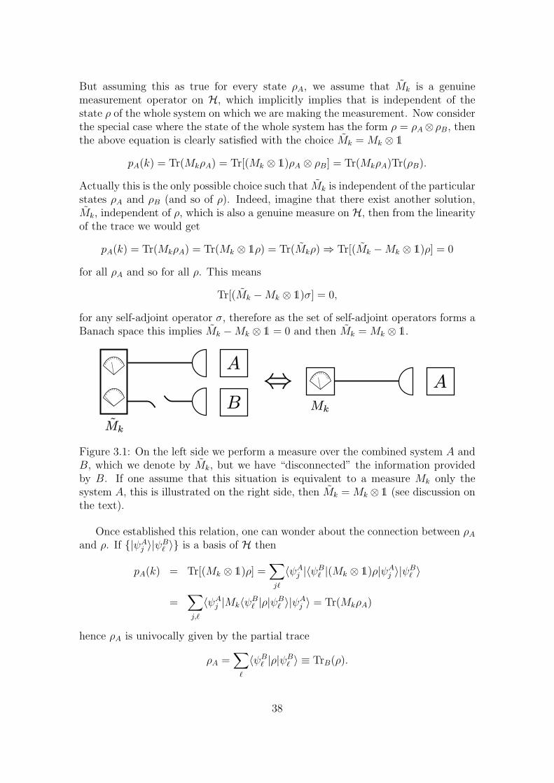
Figure 3.1: On the left side we perform a measure over the combined system A andB, which we denote by Mk, but we have “disconnected” the information providedby B. If one assume that this situation is equivalent to a measure Mk only thesystem A, this is illustrated on the right side, then Mk = Mk ⊗ 1 (see discussion onthe text).
Once established this relation, one can wonder about the connection between ρA
and ρ. If |ψAj 〉|ψB
` 〉 is a basis of H then
pA(k) = Tr[(Mk ⊗ 1)ρ] =∑
j`
〈ψAj |〈ψB
` |(Mk ⊗ 1)ρ|ψAj 〉|ψB
` 〉
=∑
j,`
〈ψAj |Mk〈ψB
` |ρ|ψB` 〉|ψA
j 〉 = Tr(MkρA)
hence ρA is univocally given by the partial trace
ρA =∑
`
〈ψB` |ρ|ψB
` 〉 ≡ TrB(ρ).
38
One important property of the partial trace operation is that, even if ρ = |ψ〉〈ψ|was pure, ρA can be mixed, this occurs if |ψ〉 is entangled. Given the total densitymatrix ρ(t0), by taking the partial trace in (3.6), the state of A at time t1, ρA(t1),is given by
ρA(t1) = TrB[U(t1, t0)ρ(t0)U†(t1, t0)]. (3.13)
If the total evolution is not factorized U(t1, t0) = UA(t1, t0) ⊗ UB(t1, t0), thenboth quantum subsystems A and B are interchanging information with each other(they are interacting), and so they are open quantum systems.
3.2.1 Dynamical maps
Let us set A as our system to study. A natural task arising from the equation (3.13)is trying to rewrite it as a dynamical map acting on HA which connects the statesof the subsystem A at times t0 and t1:
E(t1,t0) : ρA(t0) → ρA(t1),
the problem with this map is that in general it does not only depend on the globalevolution operator U(t1, t0) and on the properties of the subsystem B, but also onthe system A itself.
In order to clarify this, let us write the total initial state as the sum of twocontributions [35]:
ρ(t0) = ρA(t0)⊗ ρB(t0) + ρcorr(t0), (3.14)
where the term ρcorr(t0) is not a quantum state, satisfies
TrA[ρcorr(t0)] = TrB[ρcorr(t0)] = 0,
and contains all correlations (classical as well as quantum) between the two subsys-tems. The substitution of (3.14) in (3.13) provides
ρA(t1) = TrBU(t1, t0)[ρA(t0)⊗ ρB(t0) + ρcorr(t0)]U†(t1, t0)
=∑
i
λiTrBU(t1, t0)[ρA(t0)⊗ |ψi〉〈ψi|]U †(t1, t0)
+ TrB[U(t1, t0)ρcorr(t0)U†(t1, t0)]
=∑
α
Kα(t1, t0)ρA(t0)K†α(t1, t0) + δρ(t1, t0)
≡ E(t1,t0)[ρA(t0)], (3.15)
where α = (i, j), Ki,j(t1, t0) =√
λi〈ψj|U(t1, t0)|ψi〉 and we have used the spectral de-composition of ρB(t0) =
∑i λi|ψi〉〈ψi|. Apparently the operators Kα(t1, t0) depend
only on the global unitary evolution and on the initial state of the subsystem B, butthe inhomogeneous part δρ(t1, t0) = TrB[U(t1, t0)ρcorr(t0)U
†(t1, t0)] may no longerbe independent of ρA because of the correlation term ρcorr [36]. That is, becauseof the positivity requirement of the total density matrix ρ(t0), given some ρA(t0)
39
and ρB(t0) not any ρcorr(t0) is allowed such that ρ(t0) given by (3.14) is a positiveoperator; in the same way, given ρA(t0) and ρcorr(t0) not any ρB(t0) is allowed.
A paradigmatic example of this is the case of reduced pure states. Then thefollowing theorem is fulfilled.
3.2.1. Theorem. Let one of the reduced states of a bipartite quantum system bepure, say ρA = |ψ〉A〈ψ|, then ρcorr = 0.
Proof. Indeed, let us consider the spectral decomposition of the whole state
ρ =∑
j,k
pjk|ψAj 〉|ψB
k 〉〈ψAj |〈ψB
k |,
here |ψAj 〉 and |ψB
k 〉 are orthonormal basis of the spacesHA andHB respectively.Now we take the partial trace with respect to one system, say B,
ρA = TrB(ρ) =∑
j,k,`
pjk|ψAj 〉〈ψA
j ||〈ψB` |ψB
k 〉|2 =∑
j,k,`
pjkδ`,k|ψAj 〉〈ψA
j |
=∑
j,k
pjk|ψAj 〉〈ψA
j | =∑
j
pj|ψAj 〉〈ψA
j |,
wherepj =
∑
k
pjk.
So if ρA is a pure state then it is elementary to show that it cannot be written asnon-trivial convex combination of another two states [37, 38]; then one coefficient,say pj′ must be one, and the rest be zero pj = δjj′ . But for j 6= j′ we get that a sumof positive quantities pjk is zero, so every of them has to be zero,
pj 6=j′ = 0 =∑
k
pjk ⇔ pjk = 0, j 6= j′, ∀k,
which implies that pjk = δjj′pj′k. By inserting this in the spectral decomposition ofthe global state we get
ρ =∑
j,k
δjj′pj′k|ψAj 〉|ψB
k 〉〈ψAj |〈ψB
k |
= |ψAj′〉〈ψA
j′ | ⊗∑
k
pj′k|ψBk 〉〈ψB
k | ≡ |ψ〉A〈ψ| ⊗ ρB
and hence ρcorr = 0.2
As a result the positivity requirement forces each term in the dynamical mapto be interconnected and dependent on the state upon which they act; this means
40
that a dynamical map with some values of Kα(t1, t0) and δρ(t1, t0) can describe aphysical evolution for some states ρA(t0) and an unphysical evolution for others.
Given this fact, a possible approach to the dynamics of open quantum systemsis by means of the study of dynamical maps and their positivity domains [39–42],however that will not be our aim here.
On the other hand, the following interesting result given independently by D.Salgado et al. [43] and D. M. Tong et al. [44] provides an equivalent parametrizationof dynamical maps.
3.2.2. Theorem. Any kind of time-evolution of a quantum state ρA can always bewritten in the form
ρA(t1) =∑
α
Kα (t1, t0, ρA) ρA(t0)K†α (t1, t0, ρA) , (3.16)
where Kα (t1, t0, ρA) are operators which depend on the state ρA at time t0.
Proof. We give here a very simple proof based on an idea presented in [42]. LetρA(t0) and ρA(t1) be the states of a quantum system at times t0 and t1 respectively.Consider formally the product ρA(t0)⊗ ρA(t1) ∈ HA ⊗HA, and a unitary operationUSWAP which interchanges the states in a tensor product USWAP|ψ1〉⊗ |ψ2〉 = |ψ2〉⊗|ψ1〉, so USWAP(A⊗B)U †
SWAP = B⊗A. It is evident that the time evolution betweenρA(t0) and ρA(t1) can be written as
E(t1,t0)[ρA(t0)] = Tr2
[USWAPρA(t0)⊗ ρA(t1)U
†SWAP
]= ρA(t1),
where Tr2 denotes the partial trace with respect to the second member of the com-posed state. By taking the spectral decomposition of ρA(t1) in the central term ofthe above equation we obtain an expression of the form (3.16). 2
Note that the decomposition of (3.16) is clearly not unique. For more details seereferences [43] and [44].
It will be convenient for us to understand the dependence on ρA of the operatorsKα (t1, t0, ρA) in (3.16) as a result of limiting the action of (3.15). That is, theabove theorem asserts that restricting the action of any dynamical map (3.15) fromits positivity domain to a small enough set of states, actually to one state “ρA”if necessary, is equivalent to another dynamical map without inhomogeneous termδρ(t1, t0). However this fact can also be visualized as a by-product of the specificnonlinear features of a dynamical map as (3.15) [45, 46].
As one can already guess, the absence of the inhomogeneous part will play a keyrole. Before we move on to examine this in the next section, it is worth remarkingthat C. A. Rodrıguez et al. [47] have found that for some classes of initial separablestates ρ(t0) (the ones which have vanishing quantum discord), the dynamical map(3.16) is the same for a set of commuting states of ρA. So we can remove thedependence on ρA of Kα (t1, t0, ρA) when applying (3.16) inside of the set of statescommuting with ρA. The converse statement turns out to be also true [48].
41
3.2.2 Universal dynamical maps
We shall call a universal dynamical map (UDM) to a dynamical map which is inde-pendent of the state it acts upon, and so it describes a plausible physical evolutionfor any state ρA. In particular, since for pure ρA(t0), ρcorr(t0) = 0, according to(3.15) the most general form of a UDM is given by
ρA(t1) = E(t1,t0)[ρA(t0)] =∑
α
Kα (t1, t0) ρA(t0)K†α (t1, t0) , (3.17)
in addition, the equality
∑α
K†α (t1, t0) Kα (t1, t0) = 1 (3.18)
is fulfilled because Tr[ρA(t1)] = 1 for any initial state ρA(t0). Compare (3.16) and(3.17).
An important result is the following (see figure 3.2):
3.2.3. Theorem. A dynamical map is a UDM if only if it is induced from anextended system with the initial condition ρ(t0) = ρA(t0) ⊗ ρB(t0) where ρB(t0) isfixed for any ρA(t0).
Proof. Given such an initial condition the result is elementary to check. Con-versely, given a UDM (3.17) one can always consider the extended state ρ(t0) =ρA(t0) ⊗ |ψ〉B〈ψ|, with |ψ〉B ∈ HB fixed for every state ρA(t0), and so Kα (t1, t0) =
B〈φα|U(t1, t0)|ψ〉B, where |φα〉B is a basis of HB. Since Kα (t1, t0) only fixes a fewpartial elements of U(t1, t0) and the requirement (3.18) is consistent with the uni-tarity condition
∑α
B〈ψ|U †(t1, t0)|φα〉B〈φα|U(t1, t0)|ψ〉B = B〈ψ|U †(t1, t0)U(t1, t0)|ψ〉B
= B〈ψ|1⊗ 1|ψ〉B = 1,
such a unitary operator U(t1, t0) always exists.2
Moreover UDMs possess other interesting properties. For instance they are linearmaps, that is for ρA(t0) =
∑i λiρ
(i)A (t0) (with λi ≥ 0 and
∑i λi = 1) we have
E(t1,t0)[ρA(t0)] =∑
i
λiE(t1,t0)[ρ(i)A (t0)],
this is a simple consequence from the definition, and UDMs are positive operations(i.e. the image of a positive operator is also a positive operator).
Furthermore, a UDM holds another remarkable mathematical property. Considerthe following “Gedankenexperiment”; imagine that the system AB is actually part
42

Figure 3.2: Schematic illustration of the result presented in the theorem 3.2.3.
of another larger system ABW , where the W component does not interact with Aand B, and so it is hidden from our eyes, playing the role of a simple bystanderof the motion of A and B. Then let us consider the global dynamics of the threesubsystems. Since W is disconnected from A and B, the unitary evolution of thewhole system is of the form UAB(t1, t0)⊗UW (t1, t0), where UW (t1, t0) is the unitaryevolution of the subsystem W . If the initial state is ρABW (t0) then
ρABW (t1) = UAB(t1, t0)⊗ UW (t1, t0)ρABW (t0)U†AB(t1, t0)⊗ U †
W (t1, t0).
Note that by taking the partial trace with respect to W we get
ρAB(t1) = UAB(t1, t0)TrW
[UW (t1, t0)ρABW (t0)U
†W (t1, t0)
]U †
AB(t1, t0)
= UAB(t1, t0)TrW
[U †
W (t1, t0)UW (t1, t0)ρABW (t0)]U †
AB(t1, t0)
= UAB(t1, t0)ρAB(t0)U†AB(t1, t0),
so indeed the presence of W does not perturb the dynamics of A and B. Since weassume that the evolution of A is described by a UDM, according to the theorem3.2.3 the initial condition must be ρAB(t0) = ρA(t0) ⊗ ρB(t0), and then the mostgeneral initial condition of the global system which is compatible with that has tobe of the form ρABW (t0) = ρAW (t0)⊗ ρB(t0), where ρB(t0) is fixed for any ρAW (t0).Now let us direct our attention to the dynamics of the subsystem AW :
ρAW (t1) = TrB [UAB(t1, t0)⊗ UW (t1, t0)ρAW (t0)⊗ ρB(t0)
U †AB(t1, t0)⊗ U †
W (t1, t0)],
by using the spectral decomposition of ρB(t0), as we have already done a couple oftimes, one obtains
ρAW (t1) =∑
α
Kα (t1, t0)⊗ UW (t1, t0)ρAW (t0)K†α (t1, t0)⊗ U †
W (t1, t0)
= E(t1,t0) ⊗ U(t1,t0) [ρAW (t0)] ,
43

here E(t1,t0) is a dynamical map over the subsystem A and the operator U(t1,t0)[·] =
UW (t1, t0)[·]U †W (t1, t0) is the unitary evolution of W . As we see, the dynamical map
over the system AW is the tensor product of each individual dynamics. So if theevolution of a system is given by a UDM, E(t1,t0), then for any unitary evolutionU(t1,t0) of any dimension, E(t1,t0) ⊗ U(t1,t0) is also a UDM; and in particular is apositive-preserving operation. By writing
E(t1,t0) ⊗ U(t1,t0) =[E(t1,t0) ⊗ 1
] [1⊗ U(t1,t0)
],
as 1 ⊗ U(t1,t0) is an unitary operator, the condition for positivity-preserving assertsthat E(t1,t0)⊗1 is positive. Linear maps fulfilling this property are called completelypositive maps [49].
Since we can never dismiss the possible existence of some extra system W , out ofour control, a UDM must always be completely positive. This may be seen directlyfrom the decomposition (3.17), the reverse statement, i.e. any completely positivemap can be written as (3.17), is a famous result proved by Kraus [50]; thus theformula (3.17) is referred as the Kraus decomposition of a completely positive map.Therefore another definition of a UDM is a (trace-preserving) linear map which iscompletely positive, see for instance [11,33].
Complete positivity is a stronger requirement than positivity, the best knownexample of a map which is positive but not completely positive is the transpositionmap (see for example [33]), so it cannot represent a UDM. It is appropriate to stressthat, despite the crystal-clear reasoning about the necessity of complete positivity inthe evolution of a quantum system, it is only required if the evolution is given by aUDM, a general dynamical map may not possess this property [39–43,45,46]. Indeed,if δρ(t1, t0) 6= 0, E(t1,t0) given by (3.15) is not positive for every state, so certainly itcannot be completely positive. In addition note that if ρABW (t0) 6= ρAW (t0)⊗ρB(t0)we can no longer express the dynamical map on AW as E(t1,t0) ⊗ U(t1,t0), so thephysical requirement for complete positivity is missed.
3.2.3 Universal dynamical maps as contractions
Let us consider now the Banach space B of the trace-class operators with the tracenorm (see comments to the definition 2.1.1). Then, as we know, an operator ρ ∈ B
is a quantum state if it is positive-semidefinite, this is
〈ψ|ρ|ψ〉 ≥ 0, |ψ〉 ∈ H,
and it has trace one, which is equal to the trace norm because the positivity of itsspectrum,
ρ ∈ B is a quantum state ⇔ ρ ≥ 0 and ‖ρ‖1 = 1.
We denote the set of quantum states by B+ ⊂ B, actually the Banach space B
the smallest linear space which contains B+; in other words, any other linear spacecontaining B+ also contains to B, this is easy to check.
44
We now focus our attention in possible linear transformations on the Banachspace E(B) : B 7→ B, and in particular, as we have said in section 2.1, the set ofthese transformations is the dual Banach space B∗, in this case with the inducednorm
‖E‖1 = supρ∈B,ρ 6=0
‖E(ρ)‖1
‖ρ‖1
.
Particularly we are interested in linear maps which leave invariant the subsetB+, i.e. they connect any quantum state with another quantum state, as a UDMdoes. The following theorem holds
3.2.4. Theorem. A linear map E ∈ B∗ leaves invariant B+ if and only if it pre-serves the trace and is a contraction on B
‖E‖1 ≤ 1.
Proof. Assume that E ∈ B∗ leaves invariant the set of quantum states B+, thenit is obvious that it preserves the trace; moreover, it implies that for every positiveρ the trace norm is preserved, so ‖E(ρ)‖1 = ‖ρ‖1. Let σ ∈ B but σ /∈ B+, then bythe spectral decomposition we can split σ = σ+ − σ−, where
σ+ =
∑λj|ψj〉〈ψj|, for λi ≥ 0,
σ− = −∑λj|ψj〉〈ψj|, for λj < 0,
here λj are the eigenvalues and |ψj〉〈ψj| the corresponding eigenstates. Note thatσ+ and σ− are both positive operators. Because |ψj〉〈ψj| are orthogonal projectionswe get (in other words as ‖σ‖1 =
∑j |λj|):
‖σ‖1 = ‖σ+‖1 + ‖σ−‖1,
but then
‖E(σ)‖1 = ‖E(σ+)− E(σ−)‖1 ≤ ‖E(σ+)‖+ ‖E(σ−)‖1 = ‖σ+‖1 + ‖σ−‖1 = ‖σ‖1,
so E is a contraction.Conversely, assume that E is a contraction and preserve the trace, then for
ρ ∈ B+ we have the next chain of inequalities:
‖ρ‖1 = Tr(ρ) = Tr[E(ρ)] ≤ ‖E(ρ)‖1 ≤ ‖ρ‖1,
so ‖E(ρ)‖1 = ‖ρ‖1 and Tr[E(ρ)] = ‖E(ρ)‖1. Since ρ ∈ B+ if and only if ‖ρ‖1 =Tr(ρ) = 1, the last equality implies that E(ρ) ∈ B+ for any ρ ∈ B+. 2
This theorem was first proven by A. Kosakowski in the references [51, 52], lateron, M. B. Ruskai also analyzed the necessary condition in [53].
45
3.2.4 The inverse of a universal dynamical map
Let us come back to the scenario of dynamical maps. Given a UDM, E(t1,t0), onecan wonder if there is another UDM describing the evolution in the opposite timereversed sense E(t0,t1) in such a way that
E(t0,t1)E(t1,t0) = E−1(t1,t0)E(t1,t0) = 1.
Note, first of all, that it is quite easy to build a UDM which is not bijective (forinstance, take |ψn〉 to be an orthonormal basis of the space, then define: E(ρ) =∑
n |φ〉〈ψn|ρ|ψn〉〈φ| = Tr(ρ)|φ〉〈φ|, being |φ〉 an arbitrary fixed state), and so theinverse does not always exist. But even if it is mathematically possible to invert amap, we are going to see that in general the inverse is not another UDM.
3.2.5. Theorem. A UDM, E(t1,t0), can be inverted by another UDM if and only ifit is unitary E(t1,t0) = U(t1,t0).
Proof. The proof is easy (assuming Wigner’s theorem) but lengthy. Let usremove the temporal references to make the notation less cumbersome, so we writeE ≡ E(t1,t0). Since we have shown that UDMs are contractions on B,
‖E(σ)‖1 ≤ ‖σ‖1, σ ∈ B.
Let us suppose that there exists a UDM, E−1, which is the inverse of E ; then byapplying the above inequality twice
‖σ‖1 = ‖E−1E(σ)‖1 ≤ ‖E(σ)‖1 ≤ ‖σ‖1,
and we conclude that‖E(σ)‖1 = ‖σ‖1, ∀σ ∈ B. (3.19)
Next, note that such an invertible E would connect pure stares with pure states.Indeed, if |ψ〉〈ψ| is a pure state, suppose that E(|ψ〉〈ψ|) is not a pure state, then itcan be written as
E(|ψ〉〈ψ|) = pρ1 + (1− p)ρ2, 1 > p > 0,
for some ρ1 6= ρ2 6= E(|ψ〉〈ψ|). But taking the inverse this equation yields
|ψ〉〈ψ| = pE−1(ρ1) + (1− p)E−1(ρ2),
as E−1 is a (bijective) UDM, E−1(ρ1) 6= E−1(ρ2) are quantum states; so such adecomposition is impossible as |ψ〉〈ψ| is pure by hypothesis; and a pure state cannotbe decomposed as a non-trivial convex combination of another two states.
Now consider σ = 12(|ψ1〉〈ψ1| − |ψ2〉〈ψ2|) for two arbitrary pure states |ψ1〉〈ψ1|
and |ψ2〉〈ψ2|. Then if we calculate its eigenvalues and eigenvectors we can restringthe computation to the two dimensional subspace spanned by |ψ1〉 and |ψ2〉, because
46
any other state |ψ〉 can be decomposed as a linear combination of |ψ1〉, |ψ2〉 and|ψ⊥〉, such that σ|ψ⊥〉 = 0. Thus the eigenvalue equation reads
σ(α|ψ1〉+ β|ψ2〉) = λ(α|ψ1〉+ β|ψ2〉),
for some λ, α and β. By taking the scalar product with respect to 〈ψ1| and 〈ψ2|and solving the two simultaneous equations one finds
λ = ±1
2
√1− |〈ψ2|ψ1〉|2,
so the trace norm ‖σ‖1 =∑
j |λj| turns out to be
‖σ‖1 =√
1− |〈ψ2|ψ1〉|2. (3.20)
However, since E connects pure states with pure states,
E(σ) =1
2[E(|ψ1〉〈ψ1|)− E(|ψ2〉〈ψ2|)] =
1
2(|ψ1〉〈ψ1| − |ψ2〉〈ψ2|)
and therefore from equations (3.19) and (3.20) we conclude that
|〈ψ2|ψ1〉| = |〈ψ2|ψ1〉|.
Invoking Wigner’s theorem [31, 37], the transformation E have to be implementedby
E = V ρV †
where V is a unitary or anti-unitary operator. Finally since the effect of an anti-unitary operator involves the complex conjugation [31], that is equivalent to thetranspose of the elements in Banach space B of trace-class self-adjoint operators,which is not a completely positive map; we conclude that V has to be unitary,E(t1,t0) = U(t1,t0).
2
From another perspective, the connection between the failure of an inverse for aUDM to exist just denotes irreversibility of the universal open quantum systemsdynamics.
3.2.5 Temporal continuity. Markovian evolutions
One important problem of the dynamical maps given by UDM is related with theircontinuity in time. This can be formulated as follows: assume that we know theevolution of a system between t0 and t1, E(t1,t0), and between t1 and a posterior timet2, E(t2,t1). From the continuity of time, one could expect that the evolution be-tween t0 and t2 was given by the composition of applications, E(t2,t0) = E(t2,t1)E(t1,t0).However, the exact meaning of this equation has to be analyzed carefully.
47
Indeed, let the total initial state be ρ(t0) = ρA(t0) ⊗ ρB(t0), and the unitaryevolution operators U(t2, t1), U(t1, t0) and U(t2, t0) = U(t2, t1)U(t1, t0). Then theevolution of the subsystem A between t0 and any subsequent t is clearly given by,
E(t1,t0)[ρA(t0)] = TrB[U(t1, t0)ρA(t0)⊗ ρB(t0)U†(t1, t0)]
=∑
α
Kα (t1, t0) ρA(t0)K†α (t1, t0) ,
E(t2,t0)[ρA(t0)] = TrB[U(t2, t0)ρA(t0)⊗ ρB(t0)U†(t2, t0)]
=∑
α
Kα (t2, t0) ρA(t0)K†α (t2, t0) .
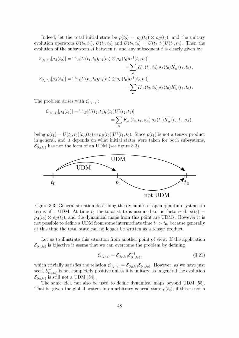
The problem arises with E(t2,t1):
E(t2,t1)[ρA(t1)] = TrB[U(t2, t1)ρ(t1)U†(t2, t1)]
=∑
α
Kα (t2, t1, ρA) ρA(t1)K†α (t2, t1, ρA) ,
being ρ(t1) = U(t1, t0)[ρA(t0)⊗ ρB(t0)]U†(t1, t0). Since ρ(t1) is not a tensor product
in general, and it depends on what initial states were taken for both subsystems,E(t2,t1) has not the form of an UDM (see figure 3.3).
Figure 3.3: General situation describing the dynamics of open quantum systems interms of a UDM. At time t0 the total state is assumed to be factorized, ρ(t0) =ρA(t0)⊗ ρB(t0), and the dynamical maps from this point are UDMs. However it isnot possible to define a UDM from some intermediate time t1 > t0, because generallyat this time the total state can no longer be written as a tensor product.
Let us to illustrate this situation from another point of view. If the applicationE(t1,t0) is bijective it seems that we can overcome the problem by defining
E(t2,t1) = E(t2,t0)E−1(t1,t0), (3.21)
which trivially satisfies the relation E(t2,t0) = E(t2,t1)E(t1,t0). However, as we have justseen, E−1
(t1,t0) is not completely positive unless it is unitary, so in general the evolution
E(t2,t1) is still not a UDM [54].The same idea can also be used to define dynamical maps beyond UDM [55].
That is, given the global system in an arbitrary general state ρ(t0), if this is not a
48
tensor product, we know that at least in some past time tinitial, before the subsystemsstarted to interact, the state was factorized ρ(tinitial) = ρA(tinitial) ⊗ ρB(tinitial). Ifwe manage to find a unitary operation U−1(t0, tinitial) which maps ρ(t0) to the stateρ(tinitial) = ρA(tinitial) ⊗ ρB(tinitial) for every reduced state ρA(t0) compatible withρ(t0), having ρB(tinitial) the same for all ρA(t0), we can describe any posterior evolu-tion from t0 to t1 as the composition of the inverse map and the UDM from tinitial tot1 as in (3.21). However to find such an unitary operator can be complicated, andit will not always exist.
On the other hand, as a difference with the dynamics of closed systems, it isclear that these difficulties arising from the continuity of the time for UDMs makeit impossible to formulate the general dynamics of open quantum systems by meansof differential equations which generate contractive families on B (i.e. families ofUDMs). However, sometimes one can write down a differential form for the evolutionfrom a fixed time origin t0, which is only a valid UDM to describe the evolutionfrom that time t0. In other words, the differential equation generates an eventuallycontractive family from t0 on B (see definition 2.4.6).
To illustrate this, consider a bijective UDM, E(t,t0), then by differentiation (with-out the aim to be very rigorous here)
dρA(t)
dt=
dE(t,t0)
dt[ρA(t0)] =
dE(t,t0)
dtE−1
(t,t0)[ρA(t)] = Lt[ρA(t)], (3.22)
where Lt =dE(t,t0)
dtE−1
(t,t0). This is the ultimate idea behind the “time convolutionless”method which will be briefly described in section 4.2.2. If the initial condition isgiven at t0, then, by construction, the solution to the above equation is ρA(t) =E(t,t0)[ρA(t0)]. Nevertheless, there is not certainty that the evolution from any otherinitial time is a UDM. Indeed, as we may guess, it is not difficult to write solutionsgiven the initial condition ρ(t1) (t1 > t0) as (3.21).
3.2.6. Definition. We will say that a quantum systems undergoes a Markovianevolution if it is described by a contractive evolution family on B and thus werecover the law of composition for the UDMs
E(t2,t0) = E(t2,t1)E(t1,t0), (3.23)
which is the quantum analogue to the Chapman-Kolgomorov equation in classicalMarkovian process (see next section 3.3.1). This property is sometimes also referredas “divisibility condition”.
Of course, no open quantum system dynamics is exactly Markovian, because aswe have already said both systems A and B develop correlations ρcorr during theirevolution and so the reduced dynamical map is not a UDM from any intermediatetime t1. However when the term which goes with ρcorr does not affect so muchthe dynamics, a Markovian model can be a good approximate description of thetime-evolution. We will analyze this deeply in section 4.1.
49
3.3 Quantum Markov process: mathematical struc-
ture
Before studying under which conditions can an open quantum system be approxi-mately described by a Markovian evolution, we examine in this section the structureand properties of quantum Markovian process.
3.3.1 Classical Markovian processes
To motivate the adopted definition of a quantum Markov process, let us recall thedefinition of classical Markov processes. More detailed explanations can be foundin [11, 56–58]; here we just sketch the most interesting properties for our purposeswithout getting too concern with mathematical rigor.
On a probability space, a stochastic process is a family of random variablesX(t), t ∈ I ⊂ R. Roughly speaking, a stochastic process is specified by a randomvariable X depending on a parameter t which usually represents the time. Assumethat I is a countable set labeled by n, then a stochastic process is a Markov processif the probability that the random variable X takes a value xn at any arbitrary timetn, is conditioned only by the value xn−1 that it took at time tn−1, and does notdepend on the values at earlier times. This condition is formulated in terms of theconditioned probabilities as follows:
p(xn, tn|xn−1, tn−1; . . . ; x0, t0) = p(xn, tn|xn−1), ∀tn ∈ I. (3.24)
This property is sometimes expressed in the following way: a Markov process doesnot have memory of the history of past values of X. They are so-named after theRussian mathematician A. Markov.
Consider now the process on a continuous interval I, then tn−1 is time infinitesi-mally close to tn. So for any t > t′ just from the definition of conditional probability
p(x, t; x′, t′) = p(x, t|x′, t′)p(x′, t′),
where p(x, t; x′, t′) is the joint probability that random variable X takes the valuex at time t and x′ at time t′. By integrating on x′ we find the relation betweenunconditional probabilities
p(x, t) =
∫dx′p(x, t|x′, t′)p(x′, t′),
and let us write it as
p(x, t) =
∫dx′K(x, t|x′, t′)p(x′, t′) with K(x, t|x′, t′) = p(x, t|x′, t′). (3.25)
The Markov process is called homogeneous if K(x, t|x′, t′) is only a function of thedifference between the two times involved K(x, t|x′, t′) = Kt−t′(x|x′).
50
Next, take the joint probability for any three consecutive times t3 > t2 > t1 andapply again the definition of conditional probability twice
p(x3, t3; x2, t2; x1, t1) = p(x3, t3|x2, t2; x1, t1)p(x2, t2; x1; t1)
= p(x3, t3|x2, t2; x1, t1)p(x2, t2|x1, t1)p(x1, t1).
The Markov condition implies that p(x3, t3|x2, t2; x1, t1) = p(x3, t3|x2, t2), then byintegrating over x2 and dividing both sides by p(x1, t1) one gets
p(x3, t3|x1, t1) =
∫dx2p(x3, t3|x2, t2)p(x2, t2|x1, t1),
which is called Chapman-Kolgomorov equation. Observe that with the notation of(3.25) this is
K(x3, t3|x1, t1) =
∫dx2K(x3, t3|x2, t2)K(x2, t2|x1, t1). (3.26)
Thinking of K(x, t|x′, t′) as propagators of the time evolution between t′ and t (3.25),equation (3.26) express that they form evolution families with that compositionlaw. Moreover, since K(x, t|x′, t′) are conditional probabilities they connect anyprobability p(x′, t′) with another probability p(x, t) so in this sense they are universal(preserve the positivity of p(x′, t′) and the normalization).
We can now draw a clear parallelism with a quantum setting. In the definitionof quantum Markov process (definition 3.2.6), the role played by the probabilitiesp(x, t) is played by the density operators ρ(t) and the role of conditional probabilitiesp(x, t|x′, t′) is played by UDMs E(t,t′), such that (3.23) is the quantum analog to theclassic Chapman-Kolgomorov equation (3.26).
3.3.2 Quantum Markov evolution as a differential equation
For positive ε, consider the difference
ρ(t + ε)− ρ(t) = [E(t+ε,0) − E(t,0)]ρ(0) = [E(t+ε,t) − 1]E(t,0)[ρ(0)] = [E(t+ε,t) − 1]ρ(t),
provided that the limit ε → 0 is well defined (we assume that the time-evolution issmooth enough). We can obtain a linear differential equation for ρ(t) (called MasterEquation)
dρ(t)
dt= lim
ε→0
ρ(t + ε)− ρ(t)
ε= lim
ε→0
[E(t+ε,t) − 1]
ερ(t) = Ltρ(t), (3.27)
where by definition the generator of the evolution is
Lt = limε→0
[E(t+ε,t) − 1]
ε.
If the quantum evolution is Markovian according to our definition 3.2.6, we maywonder what is the form of these differential equations. The answer is given by thefollowing theorem, which is the main result of the section.
51
3.3.1. Theorem. A differential equation is a Markovian master equation if andonly if it can be written in the form
dρ(t)
dt= −i[H(t), ρ(t)] +
∑
k
γk(t)
[Vk(t)ρ(t)V †
k (t)− 1
2V †
k (t)Vk(t), ρ(t)]
, (3.28)
where H(t) and Vk(t) are time-dependent operators, with H(t) self-adjoint, andγk(t) ≥ 0 for every k and time t.
Proof. For sake of simplicity we restrict the proof to finite d-dimensional systems.Let us show the necessity first (for this we follow a generalization of the argumentgiven in [59] and [11] for time-independent generators). If E(t2,t1) is a UDM for anyt2 ≥ t1 it admits a decomposition of the form
E(t2,t1)[ρ] =∑
α
Kα(t2, t1)ρK†α(t2, t1).
Actually, let Fj, j = 1, . . . , N2 be a complete orthonormal basis with respect to the
Hilbert-Schmidt inner product (Fj, Fk)HS = Tr(F †j Fk) = δjk, in such a way that we
chose FN2 = 1/√
N and the rest of operators are then traceless. Now the expansionof the Kraus operators in this basis yields
E(t2,t1)[ρ] =∑
j,k
cjk(t2, t1)FjρF †k ,
where the elements
cjk(t2, t1) =∑
α
(Fj, Kα(t2, t1))HS (Fk, Kα(t2, t1))∗HS
form a positive semidefinite matrix c(t2, t1). Indeed, for any N2-dimensional vectorv we have that
(v, c(t2, t1)v) =∑
j,k
v∗j cjk(t2, t1)vk =∑
α
∣∣∣∣∣
(∑
k
vk (Fk, Kα(t2, t1))HS
)∣∣∣∣∣
2
≥ 0.
Since this holds for any t2 ≥ t1, let us take t1 = t and t2 = t + ε, then the generatorreads
Lt(ρ) = limε→0
∑
j,k
cjk(t + ε, t)FjρF †k − 1
ε= lim
ε→0
[1
N
cN2N2(t + ε, t)−N
ερ
+1√N
N2−1∑j=1
(cjN2(t + ε, t)
εFjρ +
cN2j(t + ε, t)
ερF †
j
)
+N2−1∑
j,k=1
cjk(t + ε, t)
εFjρF †
k
]. (3.29)
52
Now, we define the time-dependent coefficients ajk(t) by
aN2N2(t) = limε→0
cN2N2(t + ε, t)−N
ε,
ajN2(t) = limε→0
cjN2(t + ε, t)
ε, j = 1, . . . , N2,
ajk(t) = limε→0
cjk(t + ε, t)
ε, j, k = 1, . . . , N2,
the following operators,
F (t) =1√N
N2−1∑j=1
ajN2(t)Fj,
G(t) =aN2N2
2N1+
1
2
[F †(t) + F (t)
],
and
H(t) =1
2i
[F †(t)− F (t)
],
which is self-adjoint. In terms of these operators the generator (3.29) can be writtenlike
Lt(ρ) = −i[H(t), ρ] + G(t), ρ+N2−1∑
j,k=1
ajk(t)FjρF †k .
Since the UDMs preserve the trace for every density matrix ρ,
0 = Tr [Lt(ρ)] = Tr
[2G(t) +
N2−1∑
j,k=1
ajk(t)F†kFj
]ρ
,
and therefore we conclude that
G(t) = −1
2
N2−1∑
j,k=1
ajk(t)F†kFj.
Note that this is nothing but the condition∑
α K†α(t2, t1)Kα(t2, t1) = 1 expressed in
differential way. Thus the generator adopts the form
Lt(ρ) = −i[H(t), ρ] +N2−1∑
j,k=1
ajk(t)
[FjρF †
k −1
2F †
kFj, ρ]
.
Finally note that because of the positive semidefiniteness of cjk(t + ε, t), the matrixajk(t), j, k = 1, . . . , N2 is also positive semidefinite, so for any t it can be diagonal-ized by mean of a unitary matrix u(t); that is,
∑
j,k
umj(t)ajk(t)u∗nk(t) = γm(t)δmn
53
where each eigenvalue is positive γm(t) ≥ 0. Introducing a new set of operatorsVk(t),
Vk(t) =N2−1∑j=1
u∗kj(t)Fj, Fj =N2−1∑
k=1
ukj(t)Vk(t)
we obtain the desired result
Lt(ρ) = −i[H(t), ρ] +∑
k
γk(t)
[Vk(t)ρV †
k (t)− 1
2V †
k (t)Vk(t), ρ]
,
with γk(t) ≥ 0,∀k, t.Assume now that a dynamics is given by a differential equation as (3.28). Since
it is a first order linear equation, there exists a continuous family of propagatorssatisfying
E(t2,t0) = E(t2,t1)E(t1,t0),
E(t,t) = 1,
for every time t2 ≥ t1 ≥ t0. It is clear that these propagators are trace preserving(as for any ρ, Tr(Ltρ) = 0). So we have to prove that for any times t2 ≥ t1 thedynamical maps E(t2,t1) are UDMs, or equivalently completely positive maps. Forthat we use the approximation formulas introduced in chapter 2; firstly the time-splitting formula (2.17) allow us to write the propagator like
E(t2,t1) = limmax |t′j+1−t′j |→0
0∏j=n−1
eLt′
j(t′j+1−t′j) (3.30)
where t2 = t′n ≥ t′n−1 ≥ . . . ≥ t′0 = t1. Next, take any element of this product
eLt′
`τ` , τ` = t′`+1 − t′` ≥ 0,
and since the constants γk(t) are positive for any time, we can write this generatorevaluated in the instant t′` as
Lt′`(·) = −i[H(t′`), (·)] +∑
k
[Vk(t
′`)(·)V †
k (t′`)−1
2V †
k (t′`)Vk(t′`), (·)
],
where Vk(t′`) =
√γk(t′`)Vk(t
′`). Now we split this generator in several parts,
Lt′` =M∑
k=0
Lk,
where
L0(·) = −i[H(t′`), (·)]−M∑m
1
2V †
m(t′`)Vm(t′`), (·), (3.31)
Lk(·) = Vk(t′`)(·)V †
k (t′`), k = 1, . . . ,M, (3.32)
54

and here M is the upper limit in the sum over k in (3.28). On one hand, differenti-ating with respect to τ one can easily check that
eL0τρ = e[−iH(t′`)−∑
k12V †k (t′`)Vk(t′`)]τρe[iH(t′`)−
∑k
12V †k (t′`)Vk(t′`)]τ
which has the form OρO†, so it is completely positive for all τ . On the other hand,for τ ≥ 0
eLkτρ =∞∑
m=0
τm
m!V m
k (t′`)ρV †mk (t′`),
has also the Kraus form∑
m OmρO†m, so it is completely positive for all k. Now
everything is ready to invoke the Lie-Trotter product formula (2.5), since
eLt′
`τ
= e(∑M
k=0 Lk)τ = limn→∞
(N∏
k=1
eLkn
)n
is the composition (infinite product) of completely positive maps eLkτ/n, it is com-pletely positive for all τ . Finally, because this is true for every instantaneous t′` the“time-splitting” formula (3.30) asserts that E(t2,t1) is completely positive for any t2and t1, because it is just another composition of completely positive maps [60].
2
This result can be taken as a global consequence of the works of A. Kossakowski[51, 52, 61] and G. Lindblad [62], who analyzed this problem for the case of time-homogeneous equations, that is, when the UDMs depend only on the differenceτ = t2 − t1, E(t2,t1) = Eτ and so they form a one-parameter semigroup (not a groupbecause the inverses are generally not a UDM, see theorem 3.2.5). As we know,under the continuity assumption, Eτ = eLτ can be defined and the generator L istime-independent, thus it has the form
Lρ(t) = −i[H, ρ(t)] +∑
k
γk
[Vkρ(t)V †
k −1
2V †
k Vk, ρ(t)]
. (3.33)
This is the result proven by Gorini, Kossakowski and Sudarshan [61] for finite di-mensional semigroups and by Lindblad [62] for infinite dimensional systems withbounded generators, that is, for uniformly continuous semigroups [23].
3.3.3 Kossakowski conditions
It is probably worthwhile to dedicate a small section to revise the original idea ofKossakowski’s seminal work [51, 52, 61], as it has clear analogies with some resultsin classical Markov processes. The route that A. Kossakowski and collaboratorsfollowed to arrive at (3.33) was to derive some analogue to the classical Markovian
55
conditions on the generator L. That is, for classical Markov process in finite dimen-sional systems, a matrix Q is the generator of an evolution stochastic matrix eQτ forany τ if only if the following conditions in its elements are satisfied:
Qii ≤ 0, ∀i, (3.34)
Qij ≥ 0, ∀i 6= j, (3.35)∑j
Qij = 0, ∀i. (3.36)
The proof can be found in [57]. To define similar conditions in the quantum case,one uses the Lumer-Phillips theorem 2.3.9, as Eτ = eLτ has to be a contractionsemigroup in the Banach space of self-adjoint matrices with respect to the tracenorm. For that aim, consider the next definition.
3.3.2. Definition. Let σ ∈ B, with spectral decomposition σ =∑
j σjPj. Wedefine the linear operator sign of σ as
sgn(σ) =∑
j
sgn(σj)Pj,
where sgn(σj) is the sign function of each eigenvalue, that is
sgn(σj) =
1, σj > 00, σj = 0
−1, σj < 0
.
3.3.3. Definition. We define the following product of two element σ, ρ ∈ B,
[σ, ρ]K = ‖σ‖Tr[sgn(σ)ρ]. (3.37)
3.3.4. Proposition. The product (3.37) is a semi-inner product. In addition it isa real number.
Proof. The proof is quite straightforward. It is evident that for the product (3.37),(2.7) and (2.8) hold. Finally (2.9) also follows easily. By introducing the spectraldecomposition of σ =
∑j σjP
σj ,
|[σ, ρ]K | = ‖σ‖∣∣∣∣∣∑
j
sgn(σj)Tr(P σj ρ)
∣∣∣∣∣ ≤ ‖σ‖∑
j
|sgn(σj)||Tr(P σj ρ)|
≤ ‖σ‖∑
j
|Tr(P σj ρ)|;
56
and we also use the spectral decomposition of ρ =∑
j ρjPρj , to obtain
∑j
|Tr(P σj ρ)| =
∑j
∣∣∣∣∣∑
k
ρkTr(P σj P ρ
k )
∣∣∣∣∣ ≤∑
k,j
|ρk||Tr(P ρj P σ
k )|
=∑
k,j
|ρk|Tr(P σj P ρ
k ) =∑
k
|ρk|Tr(P ρk ) =
∑
k
|ρk| = ‖ρ‖.
The reality of [σ, ρ]K is clear from the fact that both sgn(σ) and ρ are self-adjoint.2
Now we can formulate the equivalent to the conditions (3.34), (3.35) and (3.36) inthe quantum case.
3.3.5. Theorem (Kossakowski Conditions). A linear operator L on B (of fi-nite dimension N) is the generator of a trace preserving contraction semigroup ifand only if for every resolution of the identity P = (P1, P2, . . . , PN), 1 =
∑j Pj, the
relations
Aii(P) ≤ 0 (i = 1, 2, . . . , N), (3.38)
Aij(P) ≥ 0 (i 6= j = 1, 2, . . . , N), (3.39)N∑
i=1
Aij(P) = 0 (j = 1, 2, . . . , N) (3.40)
are satisfied, whereAij(P) = Tr[PiL(Pj)].
Proof. The condition (3.40) is just the trace preserving requirement Tr[L(σ)] = 0,σ ∈ B. We have
N∑i=1
Aij(P) =N∑i
Tr[PiL(Pj)] = Tr[L(Pj)] = 0, ∀Pj ∈ P
⇔ Tr[L(σ)] = 0, ∀σ ∈ B.
On the other hand, the theorem of Lumer-Phillips 2.3.9 asserts that
[σ,L(σ)]K ≤ 0, (3.41)
taking σ to be some projector P we obtain
Tr[P,L(P )] ≤ 0, (3.42)
so (3.38) is necessary. Furthermore (3.41) can be rewritten as
[σ,L(σ)]K =∑
k,j
sgn(σk)σjTr[PkL(Pj)] =∑
j
|σj|Tr[PjL(Pj)]
+∑
k 6=j
sgn(σk)σjTr[PkL(Pj)] ≤ 0, (3.43)
57
here we have used the spectral decomposition σ =∑
j σjPj again. By splitting(3.40) in a similar way
Tr[PjL(Pj)] = −∑
k 6=j
Tr[PkL(Pj)], for each j = 1, . . . , N.
Note that on the right hand side here the sum is just over the index k (not on j).Inserting this result in (3.43) yields
∑
k 6=j
αkjTr[PkL(Pj)] ≥ 0 (3.44)
where the sum is over the two indexes, with
αkj = |σj|[1− sgn(σk) sgn(σj)] ≥ 0.
Thus for trace-preserving semigroups the condition (3.43) is equivalent to (3.38) and(3.44). Therefore if (3.38), (3.39) and (3.40) are satisfied L is the generator of atrace preserving contraction semigroup because of (3.42) and (3.44). It only remainsto prove the necessity of (3.39), that can be seen directly from (3.44). However, itis also possible to show it from the definition of the generator:
Tr[PkL(Pj)] = limτ→0
Tr[Pk(Eτ − 1)Pj]
τ= lim
τ→0
Tr[PkEτ (Pj)]
τ≥ 0,
since Eτ (Pj) ≥ 0 as Eτ is a trace preserving and completely positive map.2
Finally from this result, one can prove (3.33). For that one realizes (similarlyto the necessity proof of theorem 3.3.1) that a trace and self-adjoint preservinggenerator can be written as
Lρ = −i[H, ρ] +N2−1∑
j,k=1
ajk
[FjρF †
k −1
2F †
kFj, ρ]
where H = H† and the coefficients ajk form a Hermitian matrix. Eτ is completelypositive (not just positive) if and only if L ⊗ 1 (in the place of L) satisfies theconditions (3.38), (3.39) and (3.40). It is easy to see [61] that this implies that ajk
is positive semidefinite, and then one obtains (3.33) by diagonalization. The matrixajk is sometimes called Kossakowski matrix [63,64].
3.3.4 Steady states of homogeneous Markov processes
In this section we give a brief introduction to the steady state properties of homoge-neous Markov processes, i.e. completely positive semigroups. This is a complicatedtopic and still an active area of research, so we only expose here some simple butimportant results.
58
3.3.6. Definition. A semigroup Eτ is relaxing if there exist a unique (steady) stateρss such that Eτ (ρss) = ρss for all τ and
limτ→∞
Eτ (ρ) = ρss,
for every initial state ρ.
Of course if one state ρss is a steady state of a semigroup Eτ then it is aneigenoperator of the operator Eτ with eigenvalue 1,
Eτ (ρss) = eLτρss = ρss,
and by differentiating it is an eigenoperator of the generator with zero eigenvalue,
L(ρss) = 0. (3.45)
If this equation admits more than one solution then the semigroup is obviously notrelaxing, and the final state will depend on the initial state, or might even oscillateinside of the set of convex combinations of solutions. However, the uniqueness ofthe solution of equation (3.45) is not a warranty for the semigroup to be relaxing.First of all let us point out the next result.
3.3.7. Theorem. A completely positive semigroup Eτ = eLτ in a finite dimensionalBanach space B has always at least one steady state, this is, there exists at least astate ρss which is a solution of (3.45).
Proof. We prove this by construction. Take any initial state ρ(0); we calculatethe average state of its evolution by (this is sometimes called “ergodic average”)
ρ = limT→∞
1
T
∫ T
0
eLτ ′ρ(0)dτ ′.
It is simple to show that the integral converges just by taking norms
limT→∞
∥∥∥∥1
T
∫ T
0
eLτρ(0)dτ
∥∥∥∥ ≤ limT→∞
1
T
∫ T
0
‖eLτ‖‖ρ(0)‖dτ ≤ 1.
Because eLτ is completely positive, it is obvious that ρ is a state. Moreover, ρ isclearly a steady state
eLτ ρ = ρ.
2
The easiest way to show the steady state properties of a finite dimensional semi-group is by writing the generator and the exponential in matrix form. In order to do
59
that, let us consider again the Hilbert-Schmidt inner product on B and a set of mu-tually orthonormal basis Fj, j = 1, . . . , N2, that is (Fj, Fk)HS = Tr(F †
j Fk) = δjk.Then the matrix elements of the generator L in that basis will be
Ljk = (Fj,LFk)HS = Tr[F †jL(Fk)].
To calculate the exponential of Ljk one uses the Jordan block form (in general Ljk
is not diagonalizable). That is, we look for a basis such that Ljk can be written asa block-diagonal matrix S−1LS = L(1) ⊕L(2) ⊕ . . .⊕L(M), of M blocks where S isthe matrix for the change of basis, and each block has the form
L(i) =
λi 1 0 . . . 0
0 λi 1. . .
......
. . . . . . . . . 0...
. . . . . . 10 . . . . . . 0 λi
.
Here λi denotes some eigenvalue of L and the size of the block coincides with itsalgebraic multiplicity ki. It is a well-know result (see for example references [23,65])that the exponential of L can be explicitly computed as
eLτ = SeL(1)τ ⊕ eL(2)τ ⊕ . . .⊕ eL(M)τS−1
= S(eλ1τeN1τ
)⊕ (eλ2τeN2τ
)⊕ . . .⊕ (eλM τeNM τ
)S−1, (3.46)
where the matrices Ni = L(i) − λi1 are nilpotent matrices, (Ni)ki = 0, and thus
their exponentials are easy to deal with. If L is a diagonalizable matrix, Ni = 0 forevery eigenvalue.
Now we move on to the principal result of this section.
3.3.8. Theorem. A completely positive semigroup is relaxing if and only if the zeroeigenvalue of L is non-degenerate and the rest of eigenvalues have negative real part.
Proof. For the “only if” part. The condition of non-degenerate zero eigenvalueof L is trivial, otherwise the semigroup has more than one steady state and is notrelaxing by definition. But even if this is true, it is necessary that the rest ofeigenvalues have negative real part. Indeed, consider some eigenvalue with purelyimaginary part L(σ) = iφσ, where σ is the associated eigenvector. By using the factthat eLτ is trace preserving
eLτ (σ) = eiφτσ ⇒ Tr[eLτ (σ)
]= Tr(σ) = eiφτTr(σ) ⇔ Tr(σ) = 0.
So we can split σ as a difference of positive operators σ = σ+ − σ−, given by itsspectral decomposition as in the proof of theorem 3.2.4. Since Tr(σ) = 0, Tr(σ+) =
60
Tr(σ−) = c, and we can write σ/c = ρ+ − ρ−, where ρ± are now quantum states.The triangle inequality with the steady state ρss reads
‖eLτ (σ/c)‖ = ‖eLτ (ρ+ − ρ−)‖ ≤ ‖eLτ (ρ+ − ρss)‖+ ‖eLτ (ρ− − ρss)‖= ‖eLτ (ρ+)− ρss‖+ ‖eLτ (ρ−)− ρss‖.
Thus if the semigroup is relaxing we obtain ‖eLτ (σ/c)‖ = 0, but this is impossibleas eLτ (σ) = eiφτσ and
‖eLτ (ρ+ − ρ−)‖ = ‖eLτ (σ/c)‖ = |eiφτ |‖(σ/c)‖ = ‖σ/c‖ > 0.
Conversely, let us denote λ1 = 0 the non-degenerate zero eigenvalue of L, sincethe remaining ones have negative real part, according to (3.46) in the limit τ →∞the matrix form of the semigroup will be
E∞ = limτ→∞
eLτ = limτ→∞
S(eλ1τ
)⊕ (eλ2τeN2τ
)⊕ . . .⊕ (eλM τeNM τ
)S−1
= S (1⊕ 0⊕ . . .⊕ 0)S−1 = SD1S−1, (3.47)
where
D1 =
1 0 · · · 00 0 · · · 0...
.... . .
...0 0 · · · 0
coincides with the projector over the eigenspace associated with the eigenvalue 1.From here it is quite simple to see that the application of E∞ on any initial state ρwritten as a vector in the basis of Fj, j = 1, . . . , N2 will give us just the steadystate. More explicitly, if ρss is the steady state, its vector representation will be
vss = [(F1, ρss)HS, . . . , (FN2 , ρss)HS]t ,
and the condition eLτρss = ρss is of course expressed in this basis as
eLτvss = vss. (3.48)
On the other side, as we already have said D1 is the projector over the eigenspaceassociated with the eigenvalue 1, which is expanded by vss, so we can write D1 =vss(vss, ·) or D1 = |vss〉〈vss| in Dirac notation.
As a particular case (τ → ∞) of (3.48), we have E∞vss = vss, after making alittle bit of algebra with this condition
E∞vss = SD1S−1vss = vss ⇒ Svss(vss,S
−1vss) = vss
⇒ Svss = 1(vss,S−1vss)
vss, (3.49)
therefore vss is eigenvector of S with eigenvalue 1(vss,S−1vss)
.
61
Finally consider any initial state ρ written as a vector vρ in the orthonormalbasis Fj, j = 1, . . . , N2. We have
limτ→∞
eLτvρ = E∞vρ = SD1S−1vρ = Svss(vss,S
−1vρ),
so using (3.49),
E∞vρ =(vss,S
−1vρ)
(vss,S−1vss)vss = C(ρ)vss, C(ρ) ≡ (vss,S
−1vρ)
(vss,S−1vss),
and in the notation of states and operators this equation reads
limτ→∞
eLτρ = C(ρ)ρss, for all ρ.
One can compute C(ρ) explicitly and find that C(ρ) = 1 for every ρ, however thisfollows from the condition that eLτ is a trace preserving semigroup.
2
There are some cases where the properties of the one dimensional eigenspace ofsteady states gives enough information about the convergence of the semigroup. Aparticular simple result is that if the unique steady state is a pure state ρss = |ψ〉〈ψ|then there are no eigenvalues of L with purely imaginary part and the semigroup isrelaxing. The proof of this statement is given by theorem 8 of reference [66].
On the other hand, it is desirable to have some condition on the structure of thegenerator which assures that the semigroup is relaxing as well as a characterizationof the steady states; there are several results on this topic (see [67–76] and referencestherein). Here we will only present an important result given by Spohn in [70].
3.3.9. Theorem (Spohn). Consider a completely positive semigroup, Eτ = eLτ ,in B with generator
Lρ = −i[H, ρ] +∑
k∈I
γk
[VkρV †
k −1
2V †
k Vk, ρ]
,
for some set of indexes I. Provided that the set Vk, k ∈ I is self-adjoint (this is,the adjoint of every element of the set is inside of the set) and the only operatorscommuting with all of them are proportional to the identity, which is expressed asVk, k ∈ I′ = c1, the semigroup Eτ is relaxing.
Proof. Since Vk, k ∈ I is self-adjoint we can consider a self-adjoint orthonormalbasis with respect to the Hilbert-Schmidt product Fj, j = 1, . . . , N2, such that asin the proof of theorem 3.3.1 we chose FN2 = 1/
√N , and so the remaining elements
are traceless. Expanding
Vk =N2−1∑m=1
vkmFm +vk,N2√
N1, (3.50)
62
we rewrite the generator as
Lρ = −i[H + H, ρ] +N2−1∑m,n=1
amn
[FmρFn − 1
2FnFm, ρ
], (3.51)
where H is the self-adjoint operator
H =∑
k∈I
γk
2i√
N
N2−1∑m=1
(vk,N2v∗km − v∗k,N2vkm
)Fm,
and the Hermitian matrix is amn =∑
k∈I γkvkmv∗kn. Now note that we can triviallychose amn to be strictly positive, for that it is enough to diagonalize again amn andignore the members in the sum of (3.51) which goes with zero eigenvalue as theydo not contribute, and write again the less dimensional matrix amn in terms of thenumbers of elements of the basis strictly necessary, say p ≤ N2 − 1
Lρ = −i[H + H, ρ] +
p∑m,n=1
amn
[FmρFn − 1
2FnFm, ρ
].
Next, consider some α > 0 to be smaller than the smallest eigenvalue of the strictlypositive amn, and divide the generator in two pieces L = L1 + L2 with
L2 = α
p∑m=1
[FmρFm − 1
2FmFm, ρ
].
It is clear that L2 is the generator of a completely positive semigroup, and the samefor L1 since amn−αδmn is still a positive semidefinite matrix. Next, for some σ ∈ B
we compute
(σ,L2(σ))HS = Tr[σL2(σ)] = α
p∑m=1
Tr[(σFm)2 − σ2F 2m]
=α
2
p∑m=1
Tr ([Fm, σ][Fm, σ]) = −α
2
p∑m=1
Tr([Fm, σ]†[Fm, σ]
) ≤ 0,
so L2 has only real eigenvalues smaller or equal to zero. Moreover for the eigenvalue0 we have Tr[σL2(σ)] = 0 which requires [Fm, σ] = 0 for m = 1, ..., p. But, becauseof the equation (3.50), it implies that [Vk, σ] = 0 for k ∈ I and therefore σ = c1 bypresupposition.
Now, let L, L1 and L2 denote the restriction of L, L1 and L2 to the subspacegenerated by Fj, j = 1, . . . , N2 − 1, this is the subspace of traceless self-adjointoperators. Then since L1 is the generator of a contracting semigroup all the eigen-values of L1 have real part smaller or equal to zero. On the other hand from theforegoing we conclude that the spectrum of L2 is composed only of strictly negative
63
real numbers, this implies that L = L1 + L2 has only eigenvalues with strictly nega-tive real part. Indeed, writing L, L1 and L2 in its matrix representation, L, L1 andL2, we can split them in their Hermitian and anti-Hermitian parts, e.g.
L = LA + iLB
where LA =(L + L†)
/2 and LB =(L− L†)
/2i are Hermitian matrices. Simi-
larly for L1 and L2. It is quite evident that the real part of the spectrum of L is
strictly negative if and only if LA is a negative definite matrix,(vσ, LAvσ
)< 0
for any σ ∈ SpanFj, j = 1, . . . , N2 − 1. But, since LA = LA1 + LA2 where
LA1 =(L1 + L†
1
)/2 and LA2 =
(L2 + L†
2
)/2, we obtain
(vσ, LAvσ
)=
(vσ, LA1vσ
)+
(vσ, LA2vσ
)< 0,
as(vσ, LA1vσ
)≤ 0 and
(vσ, LA2vσ
)< 0. Thus all the eigenvalues of L have
strictly negative real part.Finally since the eigenvalues of L are just the ones of L plus one (this is obvious
because the dimension of the subspace of traceless operators is just one less than thewhole state dimension N2), and this extra eigenvalue has to be equal to 0 becausethe theorem 3.3.7 asserts that there exists always at least one steady state. ThereforeL fulfills the conditions of the theorem 3.3.8 and the semigroup eLτ is relaxing.
2
For checking if some semigroup satisfies the conditions of this theorem it is usefulto explore if we can generate a group with the operators Vk, k ∈ I to invoke theSchur’s lemma [77].
64
Chapter 4
Microscopic derivations
4.1 Markovian case
As we have already pointed out, the dynamics of an open quantum system is notablydifferent from that of a closed system; both from practical and fundamental pointsof view. Issues so fundamental as the existence of universally valid dynamics or thecontinuity in time of these, become non-trivial matters for the evolution of openquantum systems.
Generally it would be necessary to describe the evolution in the extended closedsystem, and trace out the state at the end of the evolution. Unfortunately, inmany occasions, one of the systems is out of our control, and/or it has an infinitenumber of degrees of freedom, such that the task of calculating the associated Krausoperators can be difficult and impractical. That is the case for example of a finiteN -dimensional system coupled with an infinite dimensional one; according to Eq.(3.17), we would obtain, in principle, infinite terms in the sum. However it can beeasily shown that any completely positive map over a N -dimensional system can bewritten with at most N2 Kraus operators (of course; since the dimension of B∗ isN2, this is implicitly showed when using the Hilbert-Schmidt product in the proofof the theorem 3.3.1), so the use of the infinite terms is unnecessary.
For that reason other techniques apart from the “brute force” strategy will be-come very useful and they will be the subject of this chapter.
First, we analyze some conditions under which a UDM can be approximatelyrepresented by a quantum Markov process. We will start from a microscopic Hamil-tonian and apply some approximations leading to UDMs which fulfill the divisibilityproperty (3.23). Note that, in principle, as we have already said, the reduced evolu-tion of a quantum system is never exactly Markovian. This is because as discussedin section 3.2.5, there is always a privileged time, let say t0 where the both systemsA and B start to interact being then the global state a product ρ = ρA ⊗ ρB anddefining a UDM for ρA. At later times since the global state can no longer be fac-torized, and the dynamical map from there is not a UDM, the divisibility property(3.23) is violated.
65
4.1.1 Nakajima-Zwanzig equation
Let assume that A is our open system while B plays the role of the environment;the Hamiltonian of the whole system is given by
H = HA + HB + V, (4.1)
where HA and HB are the Hamiltonians which govern the local dynamics of A andB respectively, and V stands for the interaction between both systems.
We will follow the approach initroduced by Nakajima [78] and Zwanzig [79]using projection operators, which for instance, is also explained in [10, 11, 80]. Inthis method we define in the combined Hilbert space “system plus environment”H = HA ⊗ HB, two orthogonal projection operators, P and Q, P2 = P , Q2 = Qand PQ = QP = 0, given by
Pρ = TrB(ρ)⊗ ρB, (4.2)
Qρ = (1− P)ρ, (4.3)
where ρ ∈ H is the whole state of the system and environment and ρB ∈ HB is afixed state of the environment. In fact, we choose ρB to be the real initial state ofthe environment, this is not necessary but simplifies the computation. In addition,we assume that the system B is initially in thermal equilibrium, this is
ρB = ρth = e−βHB [Tr(e−βHB
)]−1,
where β = 1/T . Note that Pρ give all necessary information about the reducedsystem state ρA, so to know the dynamics of Pρ implies that one knows the timeevolution of the reduced system.
If we start from the von Neumann equation (3.2) for the whole system
dρ(t)
dt= −i[HA + HB + V, ρ(t)], (4.4)
and take projection operators we get
d
dtPρ(t) = −iP [HA + HB + V, ρ(t)], (4.5)
d
dtQρ(t) = −iQ[HA + HB + V, ρ(t)]. (4.6)
As usual in perturbation theory we shall work in interaction picture with respect tothe free Hamiltonians
ρ(t) = ei(HA+HB)tρ(t)e−i(HA+HB)t.
Since ρB is a thermal state and commutes with eiHBt the projection operators arepreserved under this operation
ei(HA+HB)tPρ(t)e−i(HA+HB)t = ei(HA+HB)tTrB[ρ(t)]⊗ ρBe−i(HA+HB)t
= eiHAρA(t)e−iHA ⊗ eiHBtρBe−iHBt
= ρA(t)⊗ ρB = P ρ(t),
66
because
TrB[ρ(t)] = TrB
[ei(HA+HB)tρ(t)e−i(HA+HB)t
]
= eiHAtTrB
[eiHBtρ(t)e−iHBt
]eiHAt = eiHAtTrB[ρ(t)]eiHAt = ρA(t).
For this reason equations (4.5) and (4.6) can be written in interaction picturejust like
d
dtP ρ(t) = −iP [V (t), ρ(t)], (4.7)
d
dtQρ(t) = −iQ[V (t), ρ(t)], (4.8)
which coincide of course with the result of transforming first the equation (4.4) tointeraction picture and take the projection operators P andQ over it. However, notethat these two operations do not commute if the chosen state ρB is not stationarywith respect to the local Hamiltonian HB. Then the projection operators in theinteraction picture become time-dependent Ptρ(t) = TrB[ρ(t)]⊗ ρB(t),
ei(HA+HB)tPρ(t)e−i(HA+HB)t = ρA(t)⊗ ρB(t).
A typical example of this situation is encountered for an initially squeezed environ-ment, see for example [11,13,81].
Let us use the notation V(t)· ≡ −i[V (t), ·], then by introducing the identity1 = P +Q between V(t) and ρ(t) the equations (4.7) and (4.8) may be rewritten as
d
dtP ρ(t) = PV(t)P ρ(t) + PV(t)Qρ(t), (4.9)
d
dtQρ(t) = QV(t)P ρ(t) +QV(t)Qρ(t). (4.10)
The formal integration of the first of these equations gives
P ρ(t) = Pρ(0) +
∫ t
0
dsPV(s)P ρ(s) +
∫ t
0
dsPV(s)Qρ(s), (4.11)
where we have set 0 as the origin of time without losing generality. On the otherhand, the solution of the second equation can be written formally as
Qρ(t) = G(t, 0)Qρ(0) +
∫ t
0
dsG(t, s)QV(s)P ρ(s). (4.12)
This is nothing but the operational version of variation of parameters formula forordinary differential equations (see for example [82, 83]), where the solution to thehomogeneous equation
d
dtQρ(t) = QV(t)Qρ(t)
67
is given by the propagator
G(t, s) = T e∫ t
s dt′QV(t′).
Inserting (4.12) in (4.11) yields
P ρ(t) = Pρ(0) +
∫ t
0
dsPV(s)P ρ(s) +
∫ t
0
dsPV(s)G(s, 0)Qρ(0)
+
∫ t
0
ds
∫ s
0
duPV(s)G(s, u)QV(u)P ρ(u). (4.13)
This is the integrated version of the so-called generalized Nakajima-Zwanzig equation
d
dtP ρ(t) = PV(t)P ρ(t) + PV(t)G(t, 0)Qρ(0)
+
∫ t
0
duPV(t)G(t, u)QV(u)P ρ(u). (4.14)
Next two assumptions are usually made. First one is that PV(t)P = 0, thismeans,
PV(t)Pρ = −iTrB[V (t), ρA ⊗ ρB]⊗ ρB = −i[TrB
(V (t)ρB
), ρA
]⊗ ρB = 0
for every ρ and then every ρA, which implies TrB
(V (t)ρB
)= 0. If this is not fulfilled
(which is not the case in the most practical situations), one can always define a newinteraction Hamiltonian with a shifted origin of the energy for A provided that ρB
commutes with HB [4, 84]; just choose
V ′ = V − TrB[V ρB]⊗ 1, and H ′A = HA + TrB[V ρB]⊗ 1, (4.15)
then the total Hamiltonian is the same and
TrB
[V ′(t)ρB
]= TrB
[ei(H′
A+HB)tV ′e−i(H′A+HB)tρB
]
= eiH′AtTrB[eiHBtV e−iHBtρB]e−iH′
At
− eiH′AtTrB[V ρB]e−iH′
AtTrB[eiHBtρBe−iHBt]
= eiH′AtTrB[V ρB]e−iH′
At − eiH′AtTrB[V ρB]e−iH′
At = 0,
as we wished.The second assumption consists in accepting that initially ρ(0) = ρA(0)⊗ ρB(0),
which is the necessary assumption to get a UDM. Of course some skepticism mayarise thinking that if one of the systems, say B, is not under control, there is notwarranty that this assumption is fulfilled. Nonetheless the control on the system Ais enough to assure this condition, for that it will be enough to prepare a pure statein A, for instance by making a projective measurement as argued in [85], to assureby theorem 3.2.1 that at the initial time the global system is in a product state.
68
These two assumptions make vanish the second and the third term in equation(4.13), and the integro-differential equation yields
d
dtP ρ(t) =
∫ t
0
duK(t, u)P ρ(u), (4.16)
whereK(t, u) = PV(t)G(t, u)QV(u).
If this kernel is homogeneous K(t, u) = K(t − u), which is the case for stationarystates ρB (as exemplified in next section), this equation can be formally solved bya Laplace transformation [3], but this usually turns out into an intractable problemin practice.
In order to transform this integro-differential equation in an Markovian masterequation one would wish that the integral on the right hand side of (4.16) turns intoa generator of the form of (3.28). For that aim, the first intuitive guess is to trythat K(t, u) behaves as a delta function with respect to ρ(u). For that to be truethe typical variation time τA of ρ(u) (which is only due to the interaction with Bbecause we have removed the rest of the dynamics by taking integration picture) hasto be much longer than some time τB, which characterizes the speed at which thekernel K(t, u) is decreasing when |t−u| À 1. Of course this kind of approximationsintrinsically involve some assumptions on the size of B and the “strength” of theHamiltonians, and there is in principle not warranty that the resulting differentialequation has the form of (3.28). However, several works [86–90] studied carefullytwo limiting procedures where τA/τB → ∞ so that this turns out to be the case.These two limits are
• The week coupling limit. Let us rewrite V → αV , where α accounts for thestrength of the interaction. Since for α small the variation of ρ(u) is going tobe slow, in the limit α → 0 one would get τA → ∞, and so τA/τB → ∞ forevery fixed τB. Of course for α = 0 there is not interaction, and so we will needto rescale the time appropriately before taking the limit. This is discussed inmore detail in next section 4.1.2.
• The singular coupling limit. This corresponds to somehow the opposite case;here we get τB → 0, by making K(t, u) to tend to a delta function. We willdiscuss this limit in the forthcoming section 4.1.3.
We should stress that one can construct Markovian models ad hoc which try todescribe a system from a microscopic picture without involving these procedures;see for example [91, 92]. In this sense, these two cases are sufficient conditions toget a Markovian evolution, but not necessary.
4.1.2 Weak coupling limit
As we said above, if we assume the weak coupling limit, the change of ρ(u) isnegligible within the typical time τB where the kernel K(t, u) is varying. To perform
69
this limit, consider again Eq. (4.13) under the assumptions of PV(t)P = 0 andρ(0) = ρA(0)⊗ ρB(0):
P ρ(t) = Pρ(0) + α2
∫ t
0
ds
∫ s
0
duPV(s)G(s, u)QV(u)P ρ(u), (4.17)
where we have redefined V → αV (so V → αV). Since in the interaction picturethe whole state satisfies a von Neumann equation of the form
d
dtρ(t) = −iα[V (t), ρ(t)], (4.18)
we can connect the whole state at times s and u (note u ≤ s) by the unitary solution
ρ(s) = U(s, u)ρ(u)U †(s, u) = U(s, u)ρ(u)
⇒ ρ(u) = U †(s, u)ρ(u)U(s, u) ≡ U(u, s)ρ(s).
By introducing this operator in the last term of (4.17) we find
P ρ(t) = Pρ(0) + α2
∫ t
0
ds
∫ s
0
duPV(s)G(s, u)QV(u)PU(u, s)ρ(s).
Now the term in the double integral admits an expansion in powers of α given bythe time-ordered series of
G(s, u) = T eα∫ t
s dt′QV(t′) and,
U(u, s) =[U(s, u)
]†=
[T eα
∫ su dt′V(t′)
]†= T ?eα
∫ su dt′V†(t′), (4.19)
where the adjoint is taken over every element of the expansion and T ? denotes theantichronological time-ordering operator. This is defined similarly as T in (2.14)but ordering in the opposite sense, this is, the operators evaluated at later timesappear first in the product. Thus, at lowest order we get
P ρ(t) = Pρ(0) + α2
∫ t
0
ds
∫ s
0
duPV(s)QV(u)P ρ(s) +O(α3)
= Pρ(0) + α2
∫ t
0
ds
∫ s
0
duPV(s)V(u)P ρ(s) +O(α3).
where we have used again that PV(t)P = 0. After a change of variable u → s − uand writing explicitly the projector P , and the operators V we conclude that
ρA(t) = ρA(0)− α2
∫ t
0
ds
∫ s
0
duTrB
[V (s), [V (s− u), ρA(s)⊗ ρB]
]+O(α3). (4.20)
70
Decomposition of V
In order to continue with the derivation, we write the interaction Hamiltonian as
V =∑
k
Ak ⊗Bk, (4.21)
with A†k = Ak and B†
k = Bk. Note that since V † = V , one can always chose Ak andBk to be self-adjoint. Indeed, assume that V is a sum of products of any generaloperators Xk and Yk, it will be written then like
V =n∑
k=1
X†k ⊗ Yk + Xk ⊗ Y †
k . (4.22)
Any operator can be decomposed like
Xk = X(a)k + iX
(b)k ,
where
X(a)k =
(X†k + Xk)
2, X
(b)k =
i(X†k −Xk)
2
are self-adjoint. This and the same kind of decomposition for Yk = Y(a)k + iY
(b)k
inserted in equation (4.22) gives
V =n∑
k=1
(X
(a)k − iX
(b)k
)⊗
(Y
(a)k + iY
(b)k
)
+(X
(a)k + iX
(b)k
)⊗
(Y
(a)k − iY
(b)k
)
= 2n∑
k=1
X(a)k ⊗ Y
(a)k + X
(b)k ⊗ Y
(b)k ,
so one can make the choice
Ak = 2X(a)k , Bk = 2Y
(a)k , for k = 1, . . . , n
Ak = 2X(b)k−n, Bk = 2Y
(b)k−n, for k = n + 1, . . . , 2n
to arrive at (4.21).Now we focus on the operators Ak, let us assume for the moment that the
spectrum of HA is discrete, and let |ψε〉 be an eigenstate associate with the eigenvalueε, then we define
Ak(ω) =∑
ε′−ε=ω
|ψε〉〈ψε|Ak|ψε′〉〈ψε′|,
where the sum is over every ε′ and ε such that their difference is ω. The operatorso defined is an eigenoperator of L] = i[HA, ·] with eigenvalue −iω; indeed,
L]Ak(ω) = i[HA, Ak(ω)] = i∑
ε′−ε=ω
(ε− ε′)|ψε〉〈ψε|Ak|ψε′〉〈ψε′| = −iωAk(ω).
71
As a result,L]A†
k(ω) = iωA†k(ω),
withA†
k(ω) = Ak(−ω),
and this holds for every k. In addition, it is straightforward to verify that
[HA, A†k(ω)A`(ω)] = 0. (4.23)
On the other hand, to write Ak(ω) and A†k(ω) in the interaction picture with
respect to HA is quite easy:
eL]tAk(ω) = eiHAtAk(ω)e−iHAt = e−iωtAk(ω),
eL]tA†
k(ω) = eiHAtA†k(ω)e−iHAt = eiωtA†
k(ω).
Moreover, note that∑
ω
Ak(ω) =∑
ε′,ε
|ψε〉〈ψε|Ak|ψε′〉〈ψε′| = Ak,
and similarly that ∑ω
A†k(ω) = Ak.
Therefore, by introducing these two decompositions for Ak in (4.21) and taking theinteraction picture, one gets
V (t) =∑
ω,k
e−iωtAk(ω)⊗ Bk(t) =∑
ω,k
eiωtA†k(ω)⊗ B†
k(t). (4.24)
Now, coming back to the equation (4.20) the use of the above first equality withV (s− u) and the second one with V (s) yields
ρA(t) = ρA(0) + α2
∫ t
0
ds∑
ω,ω′
∑
k,`
ei(ω′−ω)sΓsk`(ω)[A`(ω)ρA(s), A†
k(ω′)]
+ ei(ω−ω′)sΓs∗`k(ω)[A`(ω
′), ρA(s)A†k(ω)] +O(α3). (4.25)
Here we have introduced the quantities
Γsk`(ω) =
∫ s
0
dueiωuTr[Bk(s)B`(s− u)ρB
]
=
∫ s
0
dueiωuTr[Bk(u)B`ρB
], (4.26)
where the last step is justified because ρB commutes with eiHBt. Next, we rescalethe time τ = α2t and σ = α2s, obtaining
ρA(t) = ρA(τ/α2)
= ρA(0) +
∫ τ
0
dσ∑
ω,ω′
∑
k,`
ei(ω′−ω)σ/α2
Γσ/α2
k` (ω)[A`(ω)ρA(σ/α2), A†k(ω
′)]
+ ei(ω−ω′)σ/α2
Γσ/α2∗`k (ω)[A`(ω
′), ρA(σ/α2)A†k(ω)] +O(α).
72
From this equation we see that in the limit α → 0 (keeping finite τ and σ) thetime scale of change of ρ(τ/α2) is just τ . This is merely because the dependencywith α2 of ρ(τ/α2) enters only in the free evolution which we remove by takingthe interaction picture. The remaining time scale due to the interaction with theenvironment is τ , as expressed in the above equation (the integral runs from 0 toτ), so we write
limα→0
ρA(t) = limα→0
eiHAτ/α2
ρA(τ/α2)e−iHAτ/α2 ≡ ρA(τ),
and thus
ρA(τ) = ρA(0) + limα→0
∫ τ
0
dσ∑
ω,ω′
∑
k,`
ei(ω′−ω)σ/α2
Γσ/α2
k` (ω)[A`(ω)ρA(σ/α2), A†k(ω
′)]
+ ei(ω−ω′)σ/α2
Γσ/α2∗`k (ω)[A`(ω
′), ρA(σ/α2)A†k(ω)] +O(α)
= ρA(0) + limα→0
∫ τ
0
dσ∑
ω,ω′
∑
k,`
ei(ω′−ω)σ/α2
Γσ/α2
k` (ω)[A`(ω)ρA(σ), A†k(ω
′)]
+ ei(ω−ω′)σ/α2
Γσ/α2∗`k (ω)[A`(ω
′), ρA(σ)A†k(ω)]. (4.27)
Before going further in the derivation, a mathematical result which will be par-ticularly useful from now on is the following.
4.1.1. Proposition (Riemann-Lebesgue lemma). Let f(t) be integrable in [a, b]then
limx→∞
∫ b
a
eixtf(t)dt = 0.
Proof. There are several methods to prove this, here we define g(t) = f(t)[θ(t −a)− θ(t− b)] and so
∫ b
a
eixtf(t)dt =
∫ ∞
−∞eixtg(t)dt = g(x),
where g(x) denotes the Fourier transform of g(t). Now it is evident that g(t) is squareintegrable, then as the Fourier transform preserve norms [22] (this is sometimesreferred as Parseval’s theorem):
∫ ∞
−∞|g(t)|2dt =
∫ ∞
−∞|g(x)|2dx,
which implies that g(x) is also square integrable and then limx→∞ g(x) = 0.2
Because of this result (applied on the Banach space B, to be concise) in thelimit α → 0 the oscillatory factors in (4.27) with ω′ 6= ω are going to vanish. This
73
so-called secular approximation is done in the same spirit that well known rotatingwave approximation in the context of quantum optics [10,11,13,63,84]. We obtain
ρA(τ) = ρA(0) +
∫ τ
0
dσ∑
ω
∑
k,`
Γ∞k`(ω)[A`(ω)ρA(σ), A†k(ω)]
+ Γ∞∗`k (ω)[A`(ω), ρA(σ)A†k(ω)]
≡ ρA(0) +
∫ τ
0
dσL [ρA(σ)] . (4.28)
Here the coefficients are given by the one-sided Fourier transform
Γ∞k`(ω) =
∫ ∞
0
dueiωuTr[Bk(u)B`ρB
].
Correlation functions
In order to make convergent the above integrals, the environmental correlation func-
tions Tr[Bk(u)B`ρB
]have to decrease as u is increasing. However, if we also use
the corresponding eigenoperator decomposition of Bk for the Hamiltonian HB wefind
Tr[Bk(u)B`ρB
]=
∑ω
e−iωuTr [Bk(ω)B`ρB] ,
which shows that the correlation functions are periodic in u and their integral ex-tended to infinity will diverge. The only possible loophole to break the periodicityis the assumption that the system B has infinite degrees of freedom, in such a waythat HB has a continuous spectrum. Then everything is essentially the same butthe sums are substituted by integrals, i.e. the decomposition in eigenoperators willbe
Bk =
∫ a
−a
dωBk(ω), (4.29)
where a is the maximum eigenfrequency (it can be infinite). So the correlationfunctions become
Tr[Bk(u)B`ρB
]=
∫ a
−a
dωe−iωuTr [Bk(ω)B`ρB] ,
and of course now they are not periodic as
limu→∞
Tr[Bk(u)B`ρB
]= 0,
because of the proposition (4.1.1).
74
Davies’ theorem
We have just seen that a necessary condition for the weak limit to exist is thatthe environmental system B has infinite degrees of freedom. However this is nota sufficient condition because the decreasing behavior of the correlation functionsmay be not fast enough for the one-sided Fourier transform to exist. A sufficientcondition was pointed out by Davies.
4.1.2. Theorem (Davies). If there exist some ε > 0 such that
∫ ∞
0
dt∣∣∣Tr
[Bk(t)B`ρB
]∣∣∣ (1− t)ε < ∞, (4.30)
then the weak coupling is strictly well defined (for a bounded interaction V ) and
limα→0,τ=α2t
‖E(τ,0) [ρA(0)]− eLτ [ρA(0)] ‖1 = 0
for all ρA(0) and uniformly in every finite interval [0, τ0], where E(τ,0) denotes theexact reduced dynamics in the interaction picture.
Proof. To prove the condition (4.30) is beyond the scope of this work, it wasdeveloped in [86,87]. Under (4.30) the convergency to the above result is clear fromequation (4.28) which is the integrated version of
dρA(τ)
dτ= LρA(τ) ⇒ ρA(τ) = eLτ [ρA(0)] .
2
On one hand, note that the method works because there are no eigenfrequencies,ω, arbitrary close to one another, as a result of the discreteness of the spectrum ofHA, otherwise the secular approximation is jeopardized. For the infinite dimensionalcase where this is not satisfied, recently D. Taj and F. Rossi [93] have proposedanother approximation method which substitute the secular approximation and alsoleads to a completely positive semigroup.
On the other hand, an important consequence of the secular approximation isthat it guaranties that the generator L has the correct form of a Markovian homoge-nous master equation (theorem 3.3.1). To see this, let us decompose the matricesΓ∞k`(ω) in sum of Hermitian and anti-Hermitian matrices
Γ∞k`(ω) =1
2γk`(ω) + iSk`(ω), (4.31)
where the coefficients
Sk`(ω) =1
2i[Γ∞k`(ω)− Γ∞∗`k (ω)]
75
and
γk`(ω) = Γ∞k`(ω) + Γ∞∗`k (ω)
=
∫ ∞
0
dueiωuTr[Bk(u)B`ρth
]+
∫ ∞
0
due−iωuTr[Bk(−u)B`ρth
]
=
∫ ∞
−∞dueiωuTr
[Bk(u)B`ρth
], (4.32)
form Hermitian matrices. In terms of these quantities, the generator L can bewritten as
L [ρA(τ)] = − i[HLS, ρA(τ)]
+∑
ω
∑
k,`
γk`(ω)
[A`(ω)ρA(τ)A†
k(ω)− 1
2A†
k(ω)A`(ω), ρA(τ)]
,
where the Hamiltonian part is given by
HLS =∑
ω
∑
k,`
Sk`(ω)A†k(ω)A`(ω). (4.33)
In order to prove that L has the form of a generator of a Markovian homogenousevolution, it is required just to show that the matrix γk`(ω) is positive semidefinitefor all ω. This is a consequence of the Bochner’s theorem [17,22], which asserts thatthe Fourier transform of a function of “positive type” is a positive quantity. Notethat a function f(t) is of positive type if for any tm and tn the matrix constructedas fmn = f(tm − tn) is positive semidefinite.
For any vector v we have
(v,γv) =∑
k,`
v∗kγk`(ω)v` =
∫ ∞
−∞dueiωu
∑
k,`
v∗kTr[Bk(u)B`ρth
]v`
=
∫ ∞
−∞dueiωu
∑
k,`
v∗kTr[eiHBuBke
−iHBuB`ρth
]v`
=
∫ ∞
−∞dueiωuTr
[eiHBuC†e−iHBuCρth
],
where C =∑
k Bkvk.
4.1.3. Proposition. The function f(t) = Tr[eiHBtC†e−iHBtCρth
]is of “positive
type” and then the matrix γk` is positive semidefinite (v, γv) ≥ 0.
Proof. The positivity of (v,γv) ≥ 0 follows from the Bochner’s theorem if f(t)is of “positive type” because it is its Fourier transform. For the proof of the firststatement, let us take the trace in the eigenbasis of HB (remember that the spectrumis continuous):
f(t) =
∫dε〈ϕε|eiHBtC†e−iHBtCρth|ϕε〉 =
∫dεeiεtpε〈ϕε|C†e−iHBtC|ϕε〉,
76
here we have used that
ρth|ϕε〉 =e−βε
Tr [e(−βHB)]|ϕε〉 ≡ pε|ϕε〉,
with pε ≥ 0 since ρth is a positive operator. Now introducing the identity 1 =∫dε′|ϕε′〉〈ϕε′|,
f(t) =
∫dεdε′eiεtpε〈ϕε|C†e−iHBt|ϕε′〉〈ϕε′|C|ϕε〉
=
∫dεdε′ei(ε−ε′)tpε |〈ϕε′ |C|ϕε〉|2 ;
finally we take another arbitrary vector w and the inner product
(w, fw) =∑m,n
w∗mf(tm − tn)wn
=
∫dεdε′
∑m,n
w∗mei(ε−ε′)(tm−tn)wnpε |〈ϕε′|C|ϕε〉|2
=
∫dεdε′
∣∣∣∣∣∑m
w∗mei(ε−ε′)tm
∣∣∣∣∣
2
pε |〈ϕε′|C|ϕε〉|2 ≥ 0,
because the integrand is positive in the whole domain of integration.
2
As a conclusion of these results, if for a small, but finite α, we substitute theexact reduced dynamics E(t,0) by the Markovian one eLτ = eα2Lt, the error which wemake is bounded and tends to zero as α decrease provided that the assumptions ofthe Davies’ theorem are fulfilled.
Of course one can write α2L and immediately go back to Schrodinger picture byusing the unitary operator eiHAt to obtain
dρA(t)
dt= −i[HA + α2HLS, ρA(t)] (4.34)
+ α2∑
ω
∑
k,`
γk`(ω)
[A`(ω)ρA(t)A†
k(ω)− 1
2A†
k(ω)A`(ω), ρA(t)]
.
Note that because of (4.23), the Hamiltonian HLS commutes with HA, so it justproduces a shift in the energy levels of the system A. Thus this sometimes it iscalled Lamb shift Hamiltonian. However, note that HLS is not only influencedby an environment in the vacuum state (zero temperature) but also by thermalfluctuations.
77
Explicit expressions for γk` and Sk`
We can give explicit expressions for γk` and Sk` by using the decomposition of theoperators Bk in eigenoperators. For the decay rates
γk`(ω) =
∫ ∞
−∞dueiωuTr
[Bk(u)B`ρth
]
=
∫ a
−a
dω′∫ ∞
−∞duei(ω−ω′)uTr [Bk(ω
′)B`ρth]
= 2π
∫ a
−a
dω′δ(ω − ω′)Tr [Bk(ω′)B`ρth]
= 2πTr [Bk(ω)B`ρth] , (4.35)
provided that ω ∈ (−a, a). So γk`(ω) is just proportional to the correlation functionof the eigenoperator Bk(ω) with the same frequency ω, unless this frequency is notinside of the spectrum of [HB, ·], then γk`(ω) will be zero.
To get an explicit expression for the shifts Sk` is a little bit more complicated.From (4.31) we have
Sk`(ω) = −iΓ∞k`(ω) +i
2γk`(ω),
the substitution of the decomposition in eigenoperators in Γ∞k,`(ω) and the previousresult (4.35) for γk,`(ω) yields
Sk`(ω) = −i
∫ a
−a
dω′∫ ∞
0
duei(ω−ω′)uTr [Bk(ω′)B`ρB] + πiTr [Bk(ω)B`ρth] . (4.36)
Note that the integral∫∞
0duei(ω−ω′)u in not well-defined. Similarly it happens with∫∞
−∞ duei(ω−ω′)u but we know this integral is proportional to the delta function. Themathematical theory which provides a meaningful interpretation of these integralsis the theory of distributions or generalized functions. Here we will not dwell on it,references [17,18] provide introductions and further results can be found in [94,95].For us it is enough to show that these integrals can have a meaning if we definethem as a limit of ordinary functions; for instance if we define
∫ ∞
−∞duei(ω−ω′)u = lim
ε→0+
∫ ∞
0
duei(ω−ω′)u−εu + limε→0−
∫ 0
−∞duei(ω−ω′)u+εu
by making the elementary integrals,
∫ ∞
−∞duei(ω−ω′)u = lim
ε→0+
i
(ω − ω′) + εi+ lim
ε→0−
i
εi− (ω − ω′)
= limε→0
i
(ω − ω′) + εi+
i
εi− (ω − ω′)
= limε→0
2ε
ε2 + (ω − ω′)2≡ 2πδ(ω − ω′).
78
We identify the well-known family of functions fε(ω−ω′) = επ[ε2+(ω−ω′)2]
which tend
to the delta function as ε → 0 [96] because for any (regular enough) integrablefunction g(ω)
limε→0
∫ b
a
dω′fε(ω − ω′)g(ω′) = g(ω), (a < ω < b).
So, if we do the same procedure but just with the one-sided Fourier transform∫∞0
duei(ω−ω′)u, we obtain in equation (4.36)
Sk`(ω) = limε→0+
∫ a
−a
dω′1
(ω − ω′) + εiTr [Bk(ω
′)B`ρB] + πiTr [Bk(ω)B`ρth] .
Multiplying by the complex conjugate of the denominator in the integral of the righthand side, we obtain
limε→0+
∫ a
−a
dω′Tr [Bk(ω
′)B`ρB]
(ω − ω′) + εi= lim
ε→0+
∫ a
−a
dω′ (ω−ω′)(ω−ω′)2+ε2
Tr [Bk(ω′)B`ρB]
− limε→0+
i
∫ a
−a
dω′ ε(ω−ω′)2+ε2
Tr [Bk(ω′)B`ρB]
= limε→0+
∫ a
−a
dω′ (ω−ω′)(ω−ω′)2+ε2
Tr [Bk(ω′)B`ρB]
− iπTr [Bk(ω)B`ρB] .
Therefore the last term is canceled in the shifts, which read
Sk`(ω) = limε→0+
∫ a
−a
dω′ (ω−ω′)(ω−ω′)2+ε2
Tr [Bk(ω′)B`ρB] .
Now we decompose the integration interval (−a, a) in three subintervals (−a, ω−δ),(ω − δ, ω + δ) and (ω + δ, a) and take the limit δ → 0
Sk`(ω) = limε,δ→0+
∫ ω−δ
−a
dω′ (ω−ω′)(ω−ω′)2+ε2
Tr [Bk(ω′)B`ρB]
+ limε,δ→0+
∫ a
ω+δ
dω′ (ω−ω′)(ω−ω′)2+ε2
Tr [Bk(ω′)B`ρB]
+ limε,δ→0+
∫ ω+δ
ω−δ
dω′ (ω−ω′)(ω−ω′)2+ε2
Tr [Bk(ω′)B`ρB] .
The last integral just goes to zero because for any ε as small as we want the integrandis an integrable function without singularities. Whereas, since limε→0+
(ω−ω′)(ω−ω′)2+ε2
=1
(ω−ω′) , the limiting process in δ is just the definition of the Cauchy principal value
of the integral [96]:
Sk`(ω) = limδ→0+
∫ ω−δ
−a
dω′Tr [Bk(ω
′)B`ρB]
(ω − ω′)+
∫ a
ω+δ
dω′Tr [Bk(ω
′)B`ρB]
(ω − ω′)
= P.V.
∫ a
−a
dω′Tr [Bk(ω
′)B`ρB]
(ω − ω′). (4.37)
79
In theory of distributions, this result is sometimes referred as Sochozki’s formulae[95].
Typical examples
It is not worth to dwell on examples of the application of the above results, as inthe books are plenty of them. Just for sake of comparison, we sketch some of themost common cases and the correspondence with the notation above expressed.
• Two-level system damped by a bath of harmonic oscillators. The total Hamil-tonian is
H = Hsys + Hbath + V
≡ ω0
2σz +
∫ ωmax
0
dωa†ωaω +
∫ ωmax
0
dωh(ω)(σ+aω + σ−a†ω
),
where σz is the corresponding Pauli matrix, σ± = (σx ± iσy)/2, and aω ac-
counts for the continuous bosonic operators [aω, a†ω′ ] = δ(ω − ω′), here ω isthe frequency of each mode. The upper limit ωmax is the maximum frequencypresent in the bath of harmonic oscillators, it could be infinity provided thatthe coupling function h(ω) decreases fast enough. Here we have taken the con-tinuous limit from the beginning, however it is common to do it in the courseof the computation.
The interaction Hamiltonian may be written in the form V = A1⊗B1+A2⊗B2
where it is easy to check that the system operators and their eigendecomposi-tions are given by
A1 = σx = σ+ + σ−, A1(ω0) = σ−, A1(−ω0) = σ+,
A2 = σy = i(σ+ − σ−), A2(ω0) = −iσ−, A2(−ω0) = iσ+.
Similarly for the bath operators,
B1 =
∫ ωmax
0
dωh(ω) (aω+a†ω)2
=
∫ ωmax
−ωmax
dωB1(ω),
with B1(ω) = h(ω)aω
2, B1(−ω) = h(ω)a†ω
2, and
B2 =
∫ ωmax
0
dωh(ω) i(a†ω−aω)2
=
∫ ωmax
−ωmax
dωB2(ω),
with B2(ω) = −ih(ω)aω
2, B2(−ω) = ih(ω)a†ω
2.
The decay rates are given by γk,`(ω0) = 2πTr[Bk(ω0)B`ρB], particularly
γ11(ω0) = 2πTr[B1(ω0)B1ρB]
=π
2h(ω0)
∫ ωmax
0
dωh(ω)Tr[aω0(aω + a†ω)ρB]
=π
2h2(ω0)Tr[aω0a
†ω0
ρB] =π
2J(ω0)[n(ω0) + 1].
80
Here J(ω0) = h2(ω0) is the so-called spectral density of the bath (which ac-counts for the strength of the coupling per frequency, see more in chapter 9)at frequency ω0 and n(ω0) is the mean number of bosons in the thermal stateρB of the bath with frequency ω0; i.e. the expected number of particles of theBose-Einstein statistics
n(ω0) =[e(ω0/T ) − 1
]−1,
where T is the temperature of the thermal state ρB. For the rest of the elementsone obtains essentially the same
γ(ω0) =π
2J(ω0)[n(ω0) + 1]
(1 i−i 1
).
Similarly for γk,`(−ω0),
γ(−ω0) =π
2J(ω0)n(ω0)
(1 i−i 1
).
Let us make the analog for the shifts Sk`; the first element is given by
S11(ω0) = P.V.
∫ ωmax
−ωmax
dω′Tr [B1(ω
′)B1ρB]
(ω0 − ω′)
= P.V.
∫ ωmax
0
dω′Tr [Bk(ω
′)B`ρB]
(ω0 − ω′)
+ P.V.
∫ ωmax
0
dω′Tr [Bk(−ω′)B`ρB]
(ω0 + ω′)
=1
4P.V.
∫ ωmax
0
dω′J(ω′)[n(ω′) + 1
(ω0 − ω′)+
n(ω′)(ω0 + ω′)
],
the rest of the elements are
S22(ω0) = S11(ω0),
S12(ω0) = S∗21(ω0) =i
4P.V.
∫ ωmax
0
dω′J(ω′)[n(ω′) + 1
(ω0 − ω′)− n(ω′)
(ω0 + ω′)
].
For the shifts with −ω0:
S11(−ω0) = S22(−ω0) =−1
4P.V.
∫ ωmax
0
dω′J(ω′)[n(ω′) + 1
(ω0 + ω′)+
n(ω′)(ω0 − ω′)
],
S12(−ω0) = S∗21(−ω0) =−i
4P.V.
∫ ωmax
0
dω′J(ω′)[n(ω′) + 1
(ω0 + ω′)+
n(ω′)(ω0 − ω′)
].
81
Therefore according to (4.33) the shift Hamiltonian is
HLS = P.V.
∫ ωmax
0
dω′J(ω′)n(ω′)(ω0 − ω′)
[σ+, σ−] + P.V.
∫ ωmax
0
dω′J(ω′)
(ω0 − ω′)σ+σ−
= P.V.
∫ ωmax
0
dω′J(ω′)n(ω′)(ω0 − ω′)
σz + P.V.
∫ ωmax
0
dω′J(ω′)
(ω0 − ω′)(σz + 1)
2
≡(
∆′ +∆
2
)σz,
where ∆′ is the integral depending on n(ω′) which leads to a shift due to thepresence of the thermal field (Stark-like shift), and ∆ is the second integralindependent of n(ω′) which lead to a Lamb-like shift effect. Of course theidentity 1 do not contribute to the dynamics as it commutes with any ρ, sowe can forget it.
For the total equation we immediately obtain
dρsys(t)
dt= −i
[(ω0 + ∆
2+ ∆′
)σz, ρsys(t)
]
+ Γ[n(ω0) + 1]
[σ−ρsys(t)σ+ − 1
2σ+σ−, ρsys(t)
]
+ Γn
[σ+ρsys(t)σ− − 1
2σ−σ+, ρsys(t)
],
where Γ = 2πJ(ω0).
• Harmonic oscillator damped by a bath of harmonic oscillators. This case isactually quite similar to the previous one, but the two level system is nowsubstituted by another harmonic oscillator:
H = Hsys + Hbath + V
≡ ω0a†a +
∫ ωmax
0
dωa†ωaω +
∫ ωmax
0
dωh(ω)(a†aω + aa†ω
).
The bath operators B1 and B2 are the same as above and the system operatorsare now
A1 = a† + a, A1(ω0) = a, A1(−ω0) = a†,
A2 = i(a† − a), A2(ω0) = −ia, A2(−ω0) = ia†.
Thus by mimicking the previous steps we obtain
dρsys(t)
dt= −i [(ω0 + ∆) σz, ρsys(t)]
+ Γ[n(ω0) + 1]
[aρsys(t)a
† − 1
2a†a, ρsys(t)
]
+ Γn
[a†ρsys(t)a− 1
2aa†, ρsys(t)
].
82
Note in this case that, on one hand, the Stark-like shift ∆′ does not contributebecause of the commutation rule of a and a†; and on the other hand thedimension of the system is infinite and the interaction with the environment ismediated by an unbounded operator. However as long as domain problems donot arise one expects that this is the correct approximation to the dynamics(and actually it is, see chapter 5).
• Pure dephasing of a two-level system. In this case the interaction commuteswith the system Hamiltonian and so the populations of the initial systemdensity matrix remain invariant,
H = Hsys + Hbath + V
≡ ω0
2σz +
∫ ωmax
0
dωa†ωaω +
∫ ωmax
0
dωh(ω)σz
(aω + a†ω
).
This is an interesting case to explore because it involves some subtleties, butit is exactly solvable (see for example chapter 4 of [11]). The interactionHamiltonian is decomposed as V = A ⊗ B, where A = A(ω = 0) = σz (σz iseigenoperator of [σz, ·] with zero eigenvalue!) and
B =
∫ ωmax
−ωmax
dωB(ω), with
B(ω) = h(ω)aω,B(−ω) = h(ω)a†ω,
for ω > 0.
So some problem arises when we calculate the decay rates because B(ω = 0)is not well-defined. The natural solution to this is the interpretation of theω = 0 as a limit in such a way that
γ(0) = 2π limω→0
Tr[B(ω)BρB],
but then there is a further problem because depending on which side weapproach to 0 the function Tr[B(ω)BρB] takes the value 2πJ(ω)[n(ω) + 1]for ω > 0 or 2πJ(|ω|)n(|ω|) for ω < 0. Thus the limit in principle wouldnot be well-defined, except in the high temperature limit where n(|ω|) 'n(|ω|)+1. However both limits give the same result provided that one assumeslimω→0 J(|ω|) = 0. This is a natural physical assumption because a mode with0 frequency does not have any energy and influence on the system. Thus iflimω→0 J(|ω|) = 0 we find
γ(0) = 2π limω→0
J(|ω|)n(|ω|).
Actually, since n(|ω|) goes to infinity as 1/|ω| when ω decreases, if J(|ω|) doesnot tend to zero linearly in ω (this is called Ohmic-type spectral density [15])this constant γ(0) will be either 0 or infinity. This fact restricts quite a lotthe spectral densities which can be treated for the pure dephasing problemin the weak coupling framework with significant results (which is not a majorproblem because this model is exactly solvable as we have already pointed
83
out). On the other hand, shifts do not occur because HLS ∝ σzσz = 1, andfinally the Master equations is
dρsys(t)
dt= −i
[ω0
2σz, ρsys(t)
]+ γ(0) [σzρsys(t)σz − ρsys(t)] .
Some remarks on the secular approximation and positivity preservingrequirement
As we have seen, the weak coupling limit provides a rigorous mathematical procedureto derive Markovian master equations. Nonetheless for some situations in solidstate or chemical physics, where the interactions are typically stronger than forelectromagnetic environments, it is sometimes preferred to use the perturbativetreatment without performing the secular approximation. However, this methodjeopardizes the positivity of the dynamics [97] (see also [85, 98]) and several trickshave been proposed to cure this drawback. For example, one possibility is takingin consideration just the subset of the whole possible states of the system whichremain positive in the evolution [99], or describing the evolution by the inclusion ofa “slippage” operator [100]. These proposals can be useful just in some situations;in this regard it seems they do not work well for multipartite systems [101,102].
We have already explained in detail the requirement of the complete positivityfor a universal dynamics. The option to proceed without it may be useful but risky,and actually the risk seems to be quite high as the positivity of the density matrixsupports the whole consistency of the quantum theory. We believe the secularapproximation should be used as it is mathematically correct in the weak couplinglimit. In case of the failure of a completely positive semigroup to describe correctlythe dynamics of the physical system, it is probably more appropriate the use of non-Markovian methods as the “Dynamical coarse graining” (see section 4.2.3) whichpreserves complete positivity.
Failure of the assumption of factorized dynamics
In some derivations of the weak coupling limit it is common to use the followingargument. One makes the formal integration of the von Neumann equation in theinteraction picture (4.18)
d
dtρ(t) = −iα[V (t), ρ(t)],
to give
ρ(t) = ρ(0)− iα
∫ t
0
ds[V (s), ρ(s)].
By iterating this equation twice one gets
ρ(t) = ρ(0)− iα
∫ t
0
ds[V (t), ρ(0)]− α2
∫ t
0
ds
∫ s
0
du[V (s), [V (u), ρ(u)]].
84
If we take partial trace and under the usual aforementioned assumptions of ρ(0) =
ρA(0)⊗ ρB(0), and TrB
[V (t)ρB(0)
]= 0 this equation is simplified to
ρA(t) = ρA(0)− α2
∫ t
0
ds
∫ s
0
duTrB[V (s), [V (u), ρ(u)]].
Now, one argues that the system B is typically much larger than A and so, providedthat the interaction is weak, the state of B remains unperturbed by the presenceof the A and the real whole state can be approximated as ρ(u) ≈ ρA(u) ⊗ ρB(u).By making this substitution in the above equation one arrives at equation (4.20)(modulo some small details which one can consult in most of the textbooks of the ref-erences), and henceforth proceed to derive the Markovian master equation withoutany mention to projection operators.
This method can be considered as an effective model for arriving at equation(4.20), however it does not make any sense to assume that the physical state of thesystem factorizes for all times. Otherwise how would it be possible the interactionbetween both subsystems?. Moreover, why not making the substitution ρ(u) ≈ρA(u)⊗ρB(u) directly in the von Neumann equation (4.18) instead of in its integratedand iterated version?.
The validity of the substitution ρ(u) ≈ ρA(u)⊗ ρB(u) is justified because of thefactorized initial condition and the perturbative approach of the weak coupling limit.Of course we pointed out previously that the weak coupling approach makes senseonly if the coupling is small and the environment has infinite degrees of freedom.This fits in the above argument about the size of B, but it can dismissed even bynumerical simulations (see section 5.1.2) that the real total state ρ(u) is close toρA(u) ⊗ ρB(u). It should be therefore be considered as an ansatz to arrive at thecorrect equation rather than a physical requirement on the evolution.
Steady state properties
In this section we shall analyze the steady state properties of the Markovian masterequation obtained in the weak coupling limit (4.34). The most important result isthat the thermal state of the system
ρthA =
e(−HA/T )
Tr[e(−HA/T )],
with the same temperature as the bath thermal state is a steady state. To see thisone notes that the bath correlation functions satisfies the so-called Kubo-Martin-Schwinger (KMS) condition [103], namely
〈Bk(u)B`〉 = Tr[ρthBk(u)B`
]=
1
Tr (e−βHA)Tr
[eiHB(u+iβ)Bke
−iHBuB`
]
=1
Tr (e−βHA)Tr
[B`e
iHB(u+iβ)Bke−iHB(u+iβ)e−βHB
]
= Tr[B`e
iHB(u+iβ)Bke−iHB(u+iβ)ρth
]= 〈B`Bk(u + iβ)〉. (4.38)
85
By decomposing Bk in eigenoperators B(ω′) of [HB, ·], we obtain similarly to (4.35)the following relation between their Fourier transforms
γk`(ω) =
∫ ∞
−∞dueiωuTr
[Bk(u)B`ρth
]
=
∫ ∞
−∞dueiωuTr
[B`Bk(u + iβ)ρth
]
=
∫ a
−a
dω′eβω′∫ ∞
−∞duei(ω−ω′)uTr [B`Bk(ω
′)ρth]
= 2π
∫ a
−a
dω′eβω′δ(ω − ω′)Tr [B`Bk(ω′)ρth]
= 2πeβωTr [B`Bk(ω)ρth] = 2πeβω
Tr[B†
k(ω)B`ρth
]∗
= 2πeβω Tr [Bk(−ω)B`ρth]∗= eβωγ∗k`(−ω) = eβωγ`k(−ω). (4.39)
On the other hand, since A(ω′) are eigenoperators of [HA, ·] one easily obtains therelations
ρthA Ak(ω) = eβωAk(ω)ρth
A , (4.40)
ρthA A†
k(ω) = e−βωA†k(ω)ρth
A . (4.41)
Now one can check thatdρth
A
dt= 0 according to equation (4.34). Indeed, it is obvious
that ρthA commutes with the Hamiltonian part and for the remaining one, we have
dρthA
dt=
∑ω
∑
k,`
γk`(ω)
[A`(ω)ρth
A A†k(ω)− 1
2A†
k(ω)A`(ω), ρthA
]
=∑
ω
∑
k,`
γk`(ω)[e−βωA`(ω)A†
k(ω)ρthA − A†
k(ω)A`(ω)ρthA
]
=∑
ω
∑
k,`
[γk`(ω)e−βωA†
`(−ω)Ak(−ω)− γk`(ω)A†k(ω)A`(ω)
]ρth
A
=∑
ω
∑
k,`
[γ`k(−ω)A†
`(−ω)Ak(−ω)− γk`(ω)A†k(ω)A`(ω)
]ρth
A = 0,
as the sum in ω is goes from −ωmax to ωmax for some maximum difference betweenenergies ωmax. This proves that ρth
A is a steady state. Of course this does not impliesthe convergency of any initial state to it (an example is the pure dephasing equationderived in section 4.1.2), sufficient conditions for that were given in the section 3.3.4.
4.1.3 Singular coupling limit
As explained in section 4.1.1, the singular coupling limit is somehow the comple-mentary situation to the weak coupling limit, since in this case we get τB → 0 by
86
making the correlation functions to tend to a delta function. However, as a differ-ence with the weak coupling limit, the singular coupling limit is not so useful inpractice because as its own name denotes, it requires some “singular” situation. Forthat reason and for sake of comparison, we sketch here the ideas about this methodfrom our concepts previously defined, for more details the reader will be referred tothe literature.
There are several ways to implement the singular coupling limit, one consists inrescaling the total Hamiltonian as [11,59,63]
H = HA + α−2HB + α−1V
and perform the “singular limit” by taking α → 0. Starting from the equation (4.13)under the assumptions of PV(t)P = 0 and ρ(0) = ρA(0)⊗ρB(0) in this case we have
P ρ(t) = Pρ(0) +1
α2
∫ t
0
ds
∫ s
0
duPV(s)G(s, u)QV(u)P ρ(u). (4.42)
For a moment, let us take a look to the expression at first order in the expansion ofG(s, u):
P ρ(t) = Pρ(0) +1
α2
∫ t
0
ds
∫ s
0
duPV(s)V(u)P ρ(u) +O(α−3),
which we rewrite as
ρA(t) = ρA(0)− 1
α2
∫ t
0
ds
∫ s
0
du[V (s)[V (u)ρA(u)⊗ ρB]
]+O(α−3).
By introducing the general form of the interaction Eq. (4.21),
ρA(t) = ρA(0) +
∫ t
0
ds
∫ s
0
duCk`(s, u)[A`(u)ρA(u), Ak(s)
]
+ C∗k`(s, u)
[Ak(s), ρA(u)A`(u)
]+O(α−3), (4.43)
here the correlation functions are
Ck`(s, u) =1
α2Tr[Bk(s)B`(u)ρB].
If we assume that ρB is again some eigenstate of the free Hamiltonian we get
Ck`(s− u) =1
α2Tr[Bk(s− u)B`ρB], (4.44)
and by using the eigendecomposition (4.29) of Bk and taking into account the factorα−2 in the free Hamiltonian HB, we find
Ck`(s− u) =1
α2
∫ a
−a
dωe−iω(s−u)
α2 Tr[Bk(ω)B`ρB].
87
Because the proposition 4.1.1, in the limit α → 0 the above integral tends to zeroas a square integrable function in x = α−2(s− u). It implies that it tends to zero atleast as α2 and so we expect this convergence to be faster than the prefactor 1
α2 in thecorrelation functions. However in the peculiar case of s = u the correlation functionsgo to infinity, so indeed in this limit they tend to a delta function Ck`(s − u) ∝δ(s− u). Next, by making again the change of variable u → s− u, equation (4.43)reads
ρA(t) = ρA(0) +
∫ t
0
ds
∫ s
0
duCk`(u)[A`(s− u)ρA(s− u), Ak(s)
]
+ C∗k`(u)
[Ak(s), ρA(s− u)A`(s− u)
]+O(α−3).
Therefore in the limit of α → 0, we can substitute u by 0 in the A` operators andextend the integration to infinite without introducing an unbounded error
ρA(t) = ρA(0) +
∫ t
0
dsΓk`
[A`(s)ρA(s), Ak(s)
]
+ Γ∗`k[A`(s), ρA(s)Ak(s)
]+O(α−3),
where
Γk` =
∫ ∞
0
duCk`(u).
We may split this matrix in Hermitian γk` =∫∞0
duCk`(u) and anti-Hermitian partiSk` as in equation (4.31), and differentiate to obtain
dρA(t)
dt= − i[HLS(t), ρ(t)]
+ γk`
[A`(t)ρA(t)Ak(t)− 1
2
Ak(t)A`(t), ρA(t)
]+O(α−3),
where HLS(t) =∑
k,` Sk`Ak(t)A`(t). Since γk` is just the same expression as in (4.32)with ω = 0 it is always a positive semidefinite matrix and up to second order theevolution equation has the form of a Markovian master equation. However, fromthe former it is not clear what happens with the higher order terms; a completetreatment of them can be found in [88–90], where it is proven that they vanish.The idea behind this fact is that by using the property that for a Gaussian state(which ρB is assumed to be) the correlation functions of any order can be written asa sum of products of two time correlation functions (4.44). Particularly odd ordercorrelation functions vanish because of the condition PV(t)P = 0, and we obtaina product of deltas for even order. Actually the expansion is left only with thoseproducts in which some time arguments appear in “overlapping order” such as
δ(t1 − t3)δ(t2 − t4),
for t4 ≥ t3 ≥ t2 ≥ t1, and so because of the time ordered integration in the expansionof G(s, u) they do not give any contribution.
88
Finally by coming back to Schrodinger picture we obtain that in the singularcoupling limit
dρA(t)
dt= − i[HA + HLS, ρ(t)]
+ γk`
[A`ρA(t)Ak − 1
2AkA`, ρA(t)
],
note that HLS =∑
k,` Sk`AkA` does not commute in general with HA.
Despite the singular coupling limit is not very realistic, it is possible to findeffective equations for the evolution in which self-adjoint operators Ak also appear.For example under interactions with classic stochastic external fields [88] or in thestudy of the continuous measurement processes [11,104].
4.1.4 Extensions of the weak coupling limit
Here we will discuss briefly some extensions of the weak coupling limit for interactingsystems, the reader can consult further details of these situations in the examplesanalyzed in section 5.2.
Weak coupling for multipartite systems
Consider two equal (for simplicity) quantum systems and some environment, suchthat the total Hamiltonian is given by
H = HA1 + HA2 + HE + αV.
Here HA1 (HA2) is the free Hamiltonian of the subsystem 1 (2), HE is the free Hamil-tonian of the environment and αV denotes the interaction between the subsystemsand the environment. This interaction term can be written as V =
∑k A
(1)k ⊗Bk +
A(2)k ⊗Bk, where A
(1)k (A
(2)k ) are operators acting on the subsystem 1 (2), and Bk on
the environment. So the weak coupling limit for the whole state of both subsystemsρ12 leads to a Markovian master equation like
dρ12(t)
dt= −i[HA1 + HA2 + α2HLS, ρ12(t)] (4.45)
+ α2∑
ω
∑
k,`
γk`(ω)
[A`(ω)ρ12(t)A
†k(ω)− 1
2A†
k(ω)A`(ω), ρ12(t)]
,
where Ak(ω) are linear combinations of A(1)k and A
(2)k decomposed in eigenoperators
of [HA1 + HA2, ·]. Of course the form of these operators depend on the form of thecoupling. For instance, suppose that we have two identical environments that act
89
locally on each subsystem V =∑
k A(1)k ⊗B
(1)k + A
(2)k ⊗B
(2)k then we will obtain
dρ12(t)
dt= −i
2∑j=1
[HA1 + HA2 + α2H(j)LS , ρ12(t)]
+ α2∑
ω
∑
k,`
γ(j)k` (ω)
[A
(j)` (ω)ρ12(t)A
(j)†k (ω)− 1
2A(j)†
k (ω)A(j)` (ω), ρ12(t)
].
Consider now the case in which we perturb the free Hamiltonian of the subsys-tems by an interaction term between them of the form βV12 (where β accountsfor the strength). Instead of using the interaction picture with respect to thefree evolution HA1 + HA2 + HB, the general strategy to deal with this problemis considering the interaction picture including the interaction between subsystemsHA1 + HA2 + βV12 + HB, and then proceeds with the weak coupling method.
However if β is small, one can follow a different route. First, taking the interac-tion picture with respect to HA1+HA2+HB, the evolution equation for the completesystem is
d
dtρ(t) = −iβ[V12(t), ρ(t)]− iα[V (t), ρ(t)] ≡ βV12(t)ρ(t) + αV(t)ρ(t).
Similarly as in section 4.1.1, we take projection operators
d
dtP ρ(t) = βPV12(t)ρ(t) + αPVSB(t)ρ(t), (4.46)
d
dtQρ(t) = βQV12(t)ρ(t) + αQVSB(t)ρ(t), (4.47)
and find the formal solution to the second equation
Qρ(t) = G(t, 0)Qρ(0) + β
∫ t
0
dsG(t, s)QV12(s)P ρ(s)
+α
∫ t
0
dsG(t, s)QV(s)P ρ(s), (4.48)
whereG(t, s) = T e
∫ ts dt′Q[βV12(t′)+αV(t′)].
Now the procedure is as follows, we introduce the identity 1 = P + Q just in thelast term of equation (4.46),
d
dtP ρ(t) = βPV12(t)ρ(t) + αPV(t)P ρ(t) + αPV(t)Qρ(t),
whose formal integration yields
P ρ(t) = Pρ(0) + β
∫ t
0
dsPV12(s)ρ(s) + α
∫ t
0
dsPV(s)Qρ(s), (4.49)
90

here we have used the condition PV(t)P = 0. Next we insert the formal so-lution (4.48) into the last term. By assuming again an initial factorized state“subsystems⊗enviroment” (Qρ(t0) = 0) we find
P ρ(t) = Pρ(0) + β
∫ t
0
dsPV12(s)ρ(s)
+
∫ t
0
ds
∫ s
0
duK1(s, u)P ρ(u) +
∫ t
0
ds
∫ s
0
duK2(s, u)P ρ(u),
where the kernels are
K1(s, u) = αβPV(s)G(s, u)QV12(u)P = 0,
K2(s, u) = α2PV(s)G(s, u)QV(u)P .
The first one vanishes because V12(s) commutes with P and QP = 0, and the secondkernel up to second order in α and β becomes
K2(s, u) = α2PV(s)QV(u)P +O(α3, α2β) = α2PV(s)V(u)P +O(α3, α2β).
Therefore the integrated equation of motion reads
P ρ(t) = Pρ(0) + β
∫ t
0
dsPV12(s)ρ(s)
+ α2
∫ t
0
ds
∫ s
0
duPV(s)V(u)P ρ(u) +O(α3, α2β).
If we consider small intercoupling β such that α & β, we can neglect the higherorders and the weak coupling procedure of this expression (c.f. section 4.1.2) willlead to the usual weak coupling generator with the Hamiltonian part βV12 added.This is in Schrodinger picture
dρ12(t)
dt= −i[HA1 + HA2 + βV12 + α2HLS, ρ12(t)] (4.50)
+ α2∑
ω
∑
k,`
γk`(ω)
[A`(ω)ρ12(t)A
†k(ω)− 1
2A†
k(ω)A`(ω), ρ12(t)]
.
Compare equations (4.45) and (4.50).Surprisingly, this method can provide good results also for large β under some
conditions, as discussed in section 5.2.
Weak coupling under external driving
Let us consider now a system A subject to an external time-dependent perturbationβHext(t) and weakly coupled to some environment B, in such a way that the totalHamiltonian is
H = HA + βHext(t) + HB + αV.
91
In order to derive a Markovian master equation for this system we must take intoaccount of a couple of details. First, since the Hamiltonian is time-dependent thegenerator of the master equation will also be time-dependent,
dρA(t)
dt= LtρA(t),
whose solution defines a family of propagators E(t2, t1) such that
ρS(t2) = E(t2, t1)ρS(t1),
E(t3, t1) = E(t3, t2)E(t2, t1).
This family may be contractive (i.e. Markovian inhomogeneous) or just eventuallycontractive (see section 2.4). Secondly, there is an absence of rigorous methodsto derive at a Markovian master equation (i.e. contractive family) in the weakcoupling limit when the system Hamiltonian is time-dependent, with the exceptionof adiabatic regimes of external perturbations [105, 106]. Fortunately if the Hext(t)is periodic in t one is able to obtain Markovian master equations, even though thecomplexity of the problem increases.
On one hand, if β is small, in the spirit of the previous section we can expectthat the introduction of βHext(t) just in the Hamiltonian part of the evolution wouldprovide a good approximation to the motion,
dρA(t)
dt= −i[HA + βHext(t) + α2HLS, ρA(t)] (4.51)
+ α2∑
ω
∑
k,`
γk`(ω)
[A`(ω)ρA(t)A†
k(ω)− 1
2A†
k(ω)A`(ω), ρA(t)]
.
which has the form of a Markovian master equation (3.28).On the other hand, for larger β the only loophole seems to work in the interaction
picture generated by the unitary propagator
U(t1, t0) = T e−i∫ t1
t0[HA+βHext(t′)]dt′ .
Taking t0 = 0 without loss of generality, the time-evolution equation for ρ(t) =U †(t, 0)ρ(t)U(t, 0) is
dρ(t)
dt= −iα[V (t), ρ(t)]. (4.52)
Following an analogous procedure than that in section 4.1.2 for time-independentgenerators, one immediately deals with the problem that it is not clear whether thereexists something similar to the eigenoperator decomposition of V (t) = U †(t, 0)V U(t, 0)as in (4.24). Note however that since the dependency of the operator Hext(t) with tis periodical one would obtain a differential problem for each Ak in (4.21)
dAk(t)
dt= −i[Ak(t), HA + βHext(t)]. (4.53)
92

with periodic terms. This kind of equations can be studied with the well-establishedFloquet theory (see for example [82, 83]), particularly it is possible to predict if itssolution is a periodic function. In such a case, the operator in the new picture willhave a formal decomposition similar to (4.24), Ak(t) =
∑ω Ak(ω)eiωt, where now
Ak(ω) are some operators which do not necessarily satisfy a concrete eigenvalueproblem. However note that the importance of such a decomposition is that theoperators Ak(ω) are time-independent. This allows us to follow a similar procedureto that used for time-independent Hamiltonians with the secular approximation,and we will obtain the following
dρA(t)
dt= − i[α2HLS, ρA(t)]
+ α2∑
ω
∑
k,`
γk`(ω)
[A`(ω)ρA(t)A†
k(ω)− 1
2A†
k(ω)A`(ω), ρA(t)]
,
where HLS =∑
ω
∑k,` Sk`(ω)A†
k(ω)A`(ω) of course. By coming back to Schrodingerpicture,
dρA(t)
dt= − i[HA + βHext(t) + α2HLS(t), ρA(t)]
+ α2∑
ω
∑
k,`
γk`(ω)
[A`(ω, t)ρA(t)A†
k(ω, t)− 1
2A†
k(ω, t)A`(ω, t), ρA(t)]
here Ak(ω, t) = U(t, 0)Ak(ω)U †(t, 0). For these manipulations it is very useful to de-compose (when possible) the unitary propagator as product of non-commuting expo-
nential operators U(t, 0) = e−iH0te−iHt where the transformation eiH0tH(t)e−iH0t =H remove the explicit time-dependence of the Hamiltonian.
A more systematic approach to this method based on the Floquet theory can befound for instance in the work of H. -P. Breuer and F. Petruccione [11, 107], andin [108].
There is a very important thing to note here. The change of picture given by atime-dependent Hamiltonian can affect the “strength” α of V in a non-trivial way,compared to the usual interaction picture with respect to time-independent Hamil-tonians. Typically the α becomes multiplied and/or divided for some quantities likethe frequency of the time-dependence of Hext(t), and this can jeopardize the weakcoupling limit for some singular values of this quantities. For example one may ob-tain things like “1/0” inside of V (t). A detailed study of this situation for a drivenharmonic oscillator can be found in section 5.2.2.
4.2 Non-Markovian case
The microscopic description of non-Markovian dynamics is much more involved thanthe Markovian one, and developing efficient methods to deal with it is actually an
93
active area of research nowadays. One of the reasons for this difficulty is that the al-gebraic properties like contraction semigroups and/or evolution families are lost andmore complicated structures arise, e.g. evolution families which are only eventuallycontractive. We have already mentioned the advantages of being consistent withthe UDM description if we start from a global product state. According to section3.2.3 if the evolution family E(t,s) describes the evolution from s to t and the initialglobal product state occurs at time t0, then it must be eventually contractive fromthat point, i.e. ‖E(t,t0)‖ ≤ 1 for t ≥ t0. However it is possible that ‖E(t2,t1)‖ > 1 forarbitrary t1 and t2. Up to date, there is not a clear mathematical characterizationof evolution families which are only eventually contractive and this makes it difficultto check whether some concrete model is consistent.
There are non-Markovian cases where the environment is made of a few degreesof freedom (see for example [109, 110], chapter 8, and references therein). Thisallows one to make efficient numerical simulations of the whole closed system andafter that, just tracing out the environmental degrees of freedom, we obtain thedesired evolution of the open system.
However when the environment is large, a numerical simulation is completelyinefficient, unless the number of parameters involved in the evolution can be re-duced, for example in case of Gaussian states (see chapter 5) or using numericalrenormalization group procedures [111–113]. For remaining situation, the choice ofa particular technique really depends on the context. For concreteness, we sketchjust a few of them in the following sections.
4.2.1 Integro-differential models
As we have seen in section 4.1.1 the exact evolution of a reduced system can beformally written as an integro-differential equation (4.16),
d
dtP ρ(t) =
∫ t
0
duK(t, u)P ρ(u),
with a generally very complicated kernel
K(t, u) = PV(t)G(t, u)QV(u).
Typically this kernel cannot be written in a closed form and, furthermore, theintegro-differential equation is not easily solvable. On the other hand, it is pos-sible to perform a perturbative expansion of the kernel on the strength of V(t)and proceed further than in the Markovian case, where the series is shortened atthe first non-trivial order (for an example of this see [114]). Of course, by makingthis the complete positivity of the reduced dynamics is not usually conserved; andone expects a similar accuracy for the time convolutionless method (at the sameperturbative order) explained in the next section, which is simpler to solve.
As an alternative to the exact integro-differential equation, several phenomeno-logical approaches which reduce to a Markovian evolution in some limits has been
94
proposed. For example, if L is the generator of a Markovian semigroup, an integro-differential equation can be formulated as
dρ(t)
dt=
∫ t
0
k(t− t′)L[ρ(t′)], (4.54)
where k(t− t′) is some function which accounts for “memory” effects, and simplifiesthe complicated Nakajima-Zwanzig kernel. Of course, in the limit k(t − t′) →δ(t − t′) the Markovian evolution is recovered. The possible choices for this kernelwhich assure that the solution, E(t,0), is a UDM have been studied in several works[115–117], being the exponential ansazt k(t− t′) ∝ geg(t−t′) the most popular.
Another interesting phenomenological integro-differential model is the so-calledpost-Markovian master equation, proposed by A. Shabani and D. A. Lidar [118],
dρ(t)
dt= L
∫ t
0
k(t− t′)eL(t−t′)[ρ(t′)], (4.55)
which also tends to the Markovian master equation when k(t−t′) → δ(t−t′). Furtherstudies about the application of these models and the conditions to get UDMs canbe found in [119–121].
Apart from these references, the structure of kernels which preserve completepositivity has been analyzed in [122].
We should note however that, it has been recently questioned whether thesephenomenological integro-differential equations reproduce some typical features ofnon-Markovian dynamics [123].
4.2.2 Time-convolutionless forms
The convolution in integro-differential models is usually an undesirable character-istic because even when the equation can be formulated, the methods to find itssolution are complicated. The idea of the time-convolutionless (TCL) forms consistof removing this convolution from the evolution equation to end up with an ordinarydifferential equation. Behind this technique lies the property already expressed insection 3.2.5 that a UDM, E(t,t0), can be expressed as the solution of the differentialequation (3.22)
dρA(t)
dt= Lt[ρA(t)],
with generator Lt =dE(t,t0)
dtE−1
(t,t0). In general this equation generates an evolution
family that is not contractive, ‖E(t2,t1)‖ > 1, for some t1 and t2 and so non-Markovian.However, it generates an eventually contractive family from t0 ‖E(t,t0)‖ ≤ 1, as themap starting from t0, E(t,t0), is usually assumed to be UDM by hypothesis.
To formulate this class of equations from a microscopic model is not simple, al-though it can been done exactly in some cases such as, the damped harmonic oscil-lator [124,125] or the spontaneous emission of a two level atom [126,127]. In generalrecipe is following again a perturbative approach. The details of this treatment are
95
carefully explained in the original work [128] or in some textbooks (see [10, 11] forinstance). The key ingredient is to insert the backward unitary operator U(s, t)where s ≤ t defined in (4.19), ρ(s) = U(s, t)ρ(t), into the formal solution of theQρ(t), Eq. (4.12),
Qρ(t) = G(t, 0)Qρ(0) +
∫ t
0
dsG(t, s)QV(s)PU(s, t)ρ(t).
Now, by introducing the identity 1 = P+Q between U(s, t) and ρ(t), and consideringa factorized initial condition we obtain
[1−Υ(t)]Qρ(t) = Υ(t)P ρ(t),
here
Υ(t) = α
∫ t
0
dsG(t, s)QV(s)PU(s, t),
where we have rewritten V as αV .Next, note that Υ(0) = 0 and Υ(t)|α=0 = 0, so that the operator [1−Υ(t)] may
be inverted at least for not too large couplings and/or too large t. In such a case wewould obtain
Qρ(t) = [1−Υ(t)]−1Υ(t)P ρ(t).
Introducing this in the second member of equation (4.9), the first term vanishessince PV(t)P = 0, obtaining the differential equation
dPρ(t)
dt= Lt[Pρ(t)],
whereLt = αPV(t)[1−Υ(t)]−1Υ(t)P .
We can formally write the inverse operator as a geometric series
[1−Υ(t)]−1 =∞∑
n=0
Υn(t),
and then the generator as
Lt = αPV(t)∞∑
n=1
Υn(t)P .
On the other hand, Υn(t) can be expanded in powers of α by introducing the ex-pressions of G(t, s) and U(s, t), in such a way that we can construct successiveapproximations to Lt in powers of α,
Lt =∑n=2
αnL(n)t .
96
Here the sum starts from n = 2 because at lowest order Υ(t) ' α∫ t
0dsQV(s)P so
L(2)t =
∫ t
0
dsPV(t)QV(s)P =
∫ t
0
dsPV(t)V(s)P ,
which leads actually to the differentiated version of equation (4.20), as expected atlowest order. After a little bit of algebra, the next term in the expansion turns outto be
L(3)t =
∫ t
0
ds
∫ t
s
dt1PV(t)V(t1)V(s)P ,
and further terms can be calculated in the same fashion.In addition, D. Chruscinski and A. Kossakowski [129] have recently shown the
equivalence between integro-differential equations and TCL equations. They con-nect both generators by means of a Laplace transformation showing some kind ofcomplementarity between both methods. That is, if the integral kernel is simple,the TCL generator is highly singular, and viceversa.
On the other hand, given a TCL equation and an initial condition at time t0, theproblem of knowing whether its solution E(t,t0) is a UDM, i.e. a completely positivemap, is an open question for non-Markovian regime. Note that the perturbativeexpansion at finite order of the TCL generator can generally break the completepositivity (in the same fashion as a finite perturbative expansion of a Hamiltoniandynamics breaks the unitary character). So the classification of the TCL generatorswhich are just eventually contractive from a given time t0 is an important openproblem in the field of the dynamics of open quantum systems. Partial solutionshave been given in the qubit case [130] and in the case of commutative generatorsLt [131, 132]. For this latter case [Lt1 ,Lt2 ] = 0, for all t1 and t2, so that the timeordering operator has no effect and the solution is given by
E(t,t0) = e∫ t
t0Lt′dt′
.
Therefore, certainly E(t,t0) is completely positive if and only if∫ t
t0Lt′dt′ has the
standard form (3.33) for every final t.
4.2.3 Dynamical coarse graining method
The dynamical coarse-graining method was recently proposed by G. Schaller and T.Brandes [133,134] as a way to avoid the secular approximation under weak couplingwhile keeping the complete positivity in the dynamics. Later on this method hasbeen used in other works [135, 136]. Here we briefly explain the main idea andresults.
Consider the total Hamiltonian (4.1) and the usual product initial state ρ(0) =ρA(0)⊗ρB, where ρB is a stationary state of the environment. At interaction picturethe reduced state of the system at time t as a function of the total initial state is
ρA(t) = TrB
[U(t, 0)ρA(0)⊗ ρBU †(t, 0)
], (4.56)
97
where
U(t, 0) = T e−iα∫ t0 V (t′)dt′ ,
is the unitary propagator, and α again denotes the strength of the interaction. Nextwe introduce the expansion of the propagator up to the first non-trivial order inequation (4.56)
ρA(t) = ρA(0)− α2
2T
∫ t
0
dt1
∫ t
0
dt2TrB
[V (t1),
[V (t2), ρA(0)⊗ ρB
]]+O(α3),
here we have assumed again that the first order vanishes Tr[V (t)ρB] = 0 like in(4.15). Let us take a closer look to structure of the double time-ordered integral
T∫ t
0
dt1
∫ t
0
dt2TrB
[V (t1),
[V (t2), ρA(0)⊗ ρB
]]
=
∫ t
0
dt1
∫ t
0
dt2θ(t1 − t2)TrB
[V (t1),
[V (t2), ρA(0)⊗ ρB
]]
+
∫ t
0
dt1
∫ t
0
dt2θ(t2 − t1)TrB
[V (t2),
[V (t1), ρA(0)⊗ ρB
]]
≡ L(2)1 [ρA(0)] + L(2)
2 [ρA(0)] + L(2)3 [ρA(0)],
where by expanding the double commutators we find the three kind of terms, L(2)1 ,
L(2)2 and L(2)
3 . The first one appears twice, it is
L(2)1
2[ρA(0)] = −
∫ t
0
dt1
∫ t
0
dt2θ(t1 − t2)TrB
[V (t1)ρA(0)⊗ ρBV (t2)
]
+θ(t2 − t1)TrB
[V (t1)ρA(0)⊗ ρBV (t2)
]
= −∫ t
0
dt1
∫ t
0
dt2[θ(t1 − t2) + θ(t2 − t1)]
TrB
[V (t1)ρA(0)⊗ ρBV (t2)
]
= −∫ t
0
dt1
∫ t
0
dt2TrB
[V (t1)ρA(0)⊗ ρBV (t2)
],
because obviously the step functions cancel each other. Taking in account the otheranalogous term (that is the corresponding to interchange t1 ↔ t2 in the doublecommutators) we can write the total contribution as
L(2)1 [ρA(0)] = −2TrB [ΛρA(0)⊗ ρBΛ] ,
where Λ =∫ t
0V (t′)dt′.
98
The second term goes like
L(2)2 [ρA(0)] =
∫ t
0
dt1
∫ t
0
dt2θ(t1 − t2)TrB
[V (t1)V (t2)ρA(0)⊗ ρB
]
+θ(t2 − t1)TrB
[V (t2)V (t1)ρA(0)⊗ ρB
]
=
∫ t
0
dt1
∫ t
0
dt2[θ(t1 − t2) + θ(t2 − t1)]
TrB
[V (t2)V (t1)ρA(0)⊗ ρB
]
+θ(t1 − t2)TrB
[V (t1), V (t2)]ρA(0)⊗ ρB
= TrB
[Λ2ρA(0)⊗ ρB
]
+
∫ t
0
dt1
∫ t
0
dt2θ(t1 − t2)TrB
[V (t1), V (t2)]ρA(0)⊗ ρB
.
And similarly the remaining term can be expressed as
L(2)3 [ρA(0)] = TrB
[ρA(0)⊗ ρBΛ2
]
−∫ t
0
dt1
∫ t
0
dt2θ(t1 − t2)TrB
ρA(0)⊗ ρB[V (t1), V (t2)]
.
Thus putting everything together ρA(t) ≡ ρA(0) + Lt[ρA(0)] +O(α3) with
Lt[ρA(0)] = −α2
2
(L(2)
1 [ρA(0)] + L(2)2 [ρA(0)] + L(2)
3 [ρA(0)])
≡ −i[H tLS, ρA(0)] +Dt[ρA(0)].
Here the self-adjoint operator H tLS is
H tLS =
α2
2i
∫ t
0
dt1
∫ t
0
dt2θ(t1 − t2)TrE
[V (t1), V (t2)]ρB
,
and the “dissipative” part is given by
Dt[ρA(0)] = α2TrB
[ΛρA(0)⊗ ρBΛ− 1
2
Λ2, ρA(0)⊗ ρB
].
By using the spectral decomposition of ρB it is immediate to check that for anyfixed t, Lt has the Kossakowski-Lindblad form (3.33).
Since at first order
ρA(t) = (1+ Lt)ρA(0) +O(α3) ' eLt
ρA(0), (4.57)
the “dynamical coarse graining method” consists of introducing a “coarse grainingtime” τ and defining a family of generators of semigroups by
Lτ ≡ Lτ
τ.
99
And the corresponding family of differential equations
ρτA(t) = Lτ ρτ
A(t),
which solutionρτ
A(t) = etLτ
ρA(0), (4.58)
will obviously coincide with (4.58) up to second order when taking τ = t, this isρτ=t
A (t) = ρA(t).Therefore we have found a family of semigroups (4.57) which have the Kossakowski-
Lindblad form for every τ and give us the answer to the evolution for a particularvalue of τ (τ = t). This implies that the complete positivity of the dynamics ispreserved as we desire. In addition, one may want to write this evolution as a TCLequation, i.e. to find the generator Lt such that the solution of
d
dtρA(t) = Lt[ρA(t)]
fulfills ρA(t) = ρtA(t). That is given as in (3.22),
Lt =
[d
dteL
tt
]e−L
tt =
[d
dteL
t
]e−L
t
.
Particularly for large times t → ∞, this generator Lt tends to the usual weakcoupling generator (4.34) (in the interaction picture). This is expected because theupper limit of the integrals in the perturbative approach will tend to infinity and thenon-secular terms ei(ω′−ω)t will disappear for large t (because of proposition 4.1.1),which is actually equivalent to what we obtain by taking the limit α → 0 in therescaled time. Details are found in [133].
100
Part II
Interacting Systems underMarkovian Dynamics
101

Chapter 5
Composite systems of harmonicoscillators
5.1 A closer look into the damped harmonic os-
cillator
Despite the weak coupling limit is mathematically well defined, from the practicalpoint of view the conditions under which these Markovian master equations arederived are not always entirely clear. In most of the literature, and particularlyin quantum optics, they generally involve informal approximations motivated by avariety of microscopic models. This makes the range of validity of these equations tobe not totally well defined. The situation becomes even worse as the complexity ofthe open system increases. In particular, it is not an easy question to decide whetherthe dynamics of a composite, possibly driven, quantum system can be described viaa Markovian master equation, and if so, in what parameter regime.
The main purpose of this section is to take closer look into the damped harmonicoscillator problem, showing in which parameter regime the Markovian master equa-tion precisely approximates the real dynamics. We leave the case of the interactingharmonic systems for the next section 5.2. To make such a study we compare theevolution generated by the Markovian master equation with the results of an exactsimulation of the unitary dynamics of system plus environment. We take advantagethat there exist a particular, but wide class of simple states, the so-called Gaussianstates, which are entirely characterized by the first and second moments of theirposition and momentum operators. The evolution inside this class of states is there-fore particularly simple to track. Next we review some of the basic properties of theGaussian states [137].
5.1.1 Gaussian states
For any system of n canonical degrees of freedom, such as n harmonic oscillators,or n modes of a field, we can combine the 2n conjugate operators corresponding to
103
position and momentum into a convenient row vector,
R = (x1, x2, ..., xn, p1, p2, ..., pn)T. (5.1)
The usual canonical commutation relations (CCR) then take the form
[Rk, Rl] = i~σkl, (5.2)
where the skew-symmetric real 2n × 2n matrix σ is called the symplectic matrix.For the choice of R above, σ is given by,
σ =
[0 1n
−1n 0
]. (5.3)
One may also choose a mode-wise ordering of the operators, R = (x1, p1, ..., xn, pn)T,in which case the symplectic matrix takes on the form,
σ =n⊕
j=1
[0 1−1 0
]. (5.4)
Canonical transformations of the vectors S : R → R′ are then the real 2n−dimensionalmatrices S which preserve the kinematic relations specified by the CCR. That is,the elements transform as R′
a = SabRb, under the restriction,
SσST = σ. (5.5)
This condition defines the real 2n-dimensional symplectic group Sp(2n,R). For anyelement S ∈ Sp(2n,R), the transformations −S, ST and S−1 are also symplecticmatrices, and the inverse can be found from S−1 = σSTσ−1. The phase spacethen adopts the structure of a symplectic vector space, where (5.4) expresses theassociated symplectic form. Rather than considering unitary operators acting ondensity matrices in a Hilbert space, we can instead think of all the quantum dynamicstaking place on the symplectic vector space. Quantum states are then representedby functions defined on phase space, the choice of which is not unique, and commonexamples include the Wigner function, Q-function and the P -function [13,81]. Oftenone has a particular benefit for a given physical problem, however for our purposeswe shall consider the (Wigner) characteristic function χρ(ξ), which we define throughthe Weyl operator
Wξ = eiξTσR, ξ ∈ R2n (5.6)
asχρ(ξ) = Tr[ρWξ]. (5.7)
Each characteristic function uniquely determines a quantum state. These are relatedthrough a Fourier-Weyl transform, and so the state ρ can be obtained as
ρ =1
(2π)2n
∫d2nξχρ(−ξ)Wξ. (5.8)
104
We then define the set of Gaussian states as those with Gaussian characteristicfunctions. Equivalent definitions based on other phase space functions also exist,but for our choice we consider characteristic functions of the form,
χρ(ξ) = χρ(0)e−14ξTCξ+DTξ, (5.9)
where C is a 2n× 2n real symmetric matrix and D ∈ R2n is a vector. Thus, a Gaus-sian characteristic function, and therefore any Gaussian state, can be completelyspecified by 2n2 + 3n real parameters. The first moments give the expectation val-ues of the canonical coordinates dj = Tr[Rjρ] and are related to D by d = σ−1D,while the second moments make up the covariance matrix defined by
Cj,k = 2Re Tr[ρ(Rj − 〈Rj〉ρ)(Rk − 〈Rk〉ρ)]. (5.10)
These are related to C by the relation C = σTCσ. It is often the case that onlythe entanglement properties of a given state are of interest. As the vector d can bemade zero by local translations in phase space, one can specify the state entirelyusing the simpler relation,
Cj,k = 2Re Tr[ρRjRk]. (5.11)
However, in this work we shall predominantly use the relation (5.10). Using thisconvention, we mention two states of particular interest; the vacuum state, and then-mode thermal state. Both take on a convenient diagonal form. In case of thevacuum this is simply the identity C = 12n, while for the thermal state the elementsare given by
Cj,k = δjk
(1 +
2
eωj/T − 1
), (5.12)
where ωj is the frequency of the jth mode, and the equilibrium temperature is givenby T .
Operations on Gaussian states
We now consider Gaussian transformations. As the Rj are self-adjoint and irre-ducible, given any real symplectic transform S, the Stone-von Neumann theoremtells us there exists a unique unitary transformation US acting on H such thatUSWξU
†S = WSξ. Of particular interest are those operators, UG, which transform
Gaussian states to Gaussian states. To this end, we consider the infinitesimal gen-erators G, of Gaussian unitaries UG = e−iεG = 1 − iεG + O(ε2). Then to preservethe (Weyl) canonical commutation relations, the generators G must have the formG =
∑2nj,k=1 gjk(RjRk − RkRj)/2 [137]. It follows that Hamiltonians quadratic in
the canonical position and momentum operators (and correspondingly the creationand annihilation operators) will be Gaussian preserving, in particular, the Hamilto-nian for n simple harmonic oscillators, H =
∑nj=1 ωja
†jaj. It is for this reason that
harmonic oscillators provide such a useful testing ground for many body systems.An additional, though simple, property worth highlighting is the action of the
partial trace. Using the expression for the density matrix (5.8), it is straightforward
105
to see the effect of the partial trace operation on the characteristic function. If wetake a mode-wise ordering of the vector R = (R1, R2), where R1 and R2 split twosubspaces of n1 and n2 conjugate variables corresponding to partitions of the statespace of ρ into H = H1 ⊗H2, then the partial trace over H2 is given by
Tr2(ρ) =1
(2π)2n1
∫d2n1ξ1χρ(−ξ1)Wξ1 . (5.13)
That is, we need only consider the characteristic function χ(ξ1) associated to the
vector ~R1. At the level of covariance matrices, we simply discard elements corre-sponding to variances including any operators in ~R2, and so the partial trace of aGaussian state will itself remain Gaussian.
Finally, we make some remarks regarding closeness of two Gaussian states. Given
ρ1 and ρ2 the fidelity between them is defined as F (ρ1, ρ2) =(Tr
√√ρ1ρ2
√ρ1
)2, and
is a measure of how close both quantum system are each other. Actually a distancemeasure can be defined as DB =
√1− F which is essentially the same as the Bures
distance [138](D2
Bures(ρ1, ρ2) = 2− 2√
F (ρ1, ρ2)). This distance will be very useful
for quantifying how well the dynamics generated by a Markovian master equationapproximate the real one.
In general the fidelity is quite difficult to compute, however in the case of Gaus-sian states Scutaru has given closed formulas in terms of the covariance matrix [139].For example, in case of one mode Gaussian states ρG1 and ρG2, with covariance ma-trices C(1) and C(2) and displacement vectors d(1) and d(2) respectively, their fidelityis given by the formula
F (ρG1, ρG2) =2√
Λ + Φ−√Φexp
[−δT
(C(1) + C(2))−1
δ], (5.14)
where Λ = det[C(1) + C(2)
], Φ = det
(C(1) − 1)det
(C(2) − 1)
and δ =(d(1) − d(2)
).
5.1.2 Damped harmonic oscillator
We now first consider a single harmonic oscillator damped by an environment con-sisting of M oscillators (see figure 5.1). We want to know under which conditionsthe Markovian master equation that we derived in section 4.1.2. To this aim we willapproach the exact dynamical equations of the whole system when M is large; thesewill be solved via computer simulation, and we can then compare this solution withthe one obtained using the master equation.
The Hamiltonian for the whole system will be given by (~ = 1)
H = Ωa†a +M∑
j=1
ωja†jaj +
M∑j=1
gj(a†aj + aa†j). (5.15)
Note that the coupling to the bath has been considered in the rotating wave approx-imation (RWA), which is a good description of the real dynamics for small dampingΩ À maxgj, j = 1, . . . , M (e.g. in the weak coupling limit) [140].
106
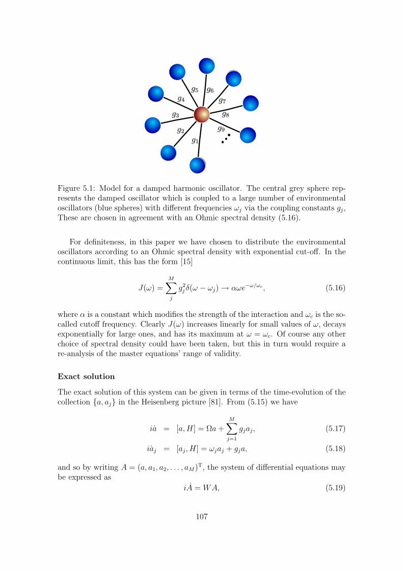
Figure 5.1: Model for a damped harmonic oscillator. The central grey sphere rep-resents the damped oscillator which is coupled to a large number of environmentaloscillators (blue spheres) with different frequencies ωj via the coupling constants gj,These are chosen in agreement with an Ohmic spectral density (5.16).
For definiteness, in this paper we have chosen to distribute the environmentaloscillators according to an Ohmic spectral density with exponential cut-off. In thecontinuous limit, this has the form [15]
J(ω) =M∑j
g2j δ(ω − ωj) → αωe−ω/ωc , (5.16)
where α is a constant which modifies the strength of the interaction and ωc is the so-called cutoff frequency. Clearly J(ω) increases linearly for small values of ω, decaysexponentially for large ones, and has its maximum at ω = ωc. Of course any otherchoice of spectral density could have been taken, but this in turn would require are-analysis of the master equations’ range of validity.
Exact solution
The exact solution of this system can be given in terms of the time-evolution of thecollection a, aj in the Heisenberg picture [81]. From (5.15) we have
ia = [a,H] = Ωa +M∑
j=1
gjaj, (5.17)
iaj = [aj, H] = ωjaj + gja, (5.18)
and so by writing A = (a, a1, a2, . . . , aM)T, the system of differential equations maybe expressed as
iA = WA, (5.19)
107
where W is the matrix
W =
Ω g1 g2 · · · gM
g1 ω1
g2 ω2...
. . .
gM ωM
, (5.20)
and the solution of the system will be given by
A(t) = TA(0), T = e−iWt. (5.21)
Analogously, the evolution of the creation operator will be
−iA† = WA† ⇒ A†(t) = T †A†(0), T † = eiWt, (5.22)
where A† = (a†, a†1, . . . , a†M)T.
We can also compute the evolution of position and momentum operators X =12(A + A†) and P = 1
2i(A− A†),
X(t) =1
2[TA(0) + T †A†(0)]
=1
2T [X(0) + iP (0)] + T †[X(0)− iP (0)]
= TRX(0)− TIP (0), (5.23)
and similarly
P (t) = TIX(0) + TRP (0), (5.24)
in these expressions, TR and TI are the self-adjoint matrices defined by
T = TR + iTI ⇒
TR = T+T †2
= cos(Wt)
TI = T−T †2i
= − sin(Wt). (5.25)
So, the time-evolution of the vector R = (x, x1, . . . , xM , p, p1, . . . , pM)T will be givenby
R(t) = MR(0) =
(TR −TI
TI TR
)R(0), (5.26)
note that the size of M is 2(M + 1)× 2(M + 1).
Due to the linearity in the couplings in H, an initial (global) Gaussian stateρG will remain Gaussian at all times t, and so we can restrict our attention to theevolution of its covariance matrix
Ci,j = 〈RiRj + RjRi〉 − 2〈Ri〉〈Rj〉. (5.27)
108
Particularly, since we are interested in just the first oscillator, we only need theevolution of the 2 × 2 submatrix Cij; i, j = 1,M + 2. The evolution of pairs ofposition and momentum operators is
〈Ri(t)Rj(t)〉 =∑
k,`
Mi,kMj,`〈Rk(0)R`(0)〉, (5.28)
and similarly for products of expectation values 〈Ri(t)〉〈Rj(t)〉. So the elements ofthe covariance matrix at time t will be
Ci,j(t) = 〈Ri(t)Rj(t) + Rj(t)Ri(t)〉 − 2〈Ri(t)〉〈Rj(t)〉=
∑
k,`
Mi,kMj,`[〈Rk(0)R`(0) + R`(0)Rk(0)〉 − 2〈Rk(0)〉〈R`(0)〉]
=∑
k,`
Mi,kMj,`Ck,`(0),
and for the first oscillator we have
C1,1(t) =∑
k,`
M1,kM1,`Ck,`(0) = (M1, CM1), (5.29)
C1,M+2(t) = CM+2,1(t) =∑
k,`
M1,kMM+2,`Ck,`(0) = (M1, CMM+2),(5.30)
CM+2,M+2(t) =∑
k,`
MM+2,kMM+2,`Ck,`(0) = (MM+2, CMM+2), (5.31)
here (·, ·) denotes the scalar product, and the vectors M1 and MM+2 are given by
M1 = (M1,1,M1,2, . . . ,M1,2M+2)T, (5.32)
MM+2 = (MM+2,1,MM+2,2, . . . ,MM+2,2M+2)T. (5.33)
Markovian master equation
The damped harmonic oscillator is a standard example for the derivation of masterequations (see for example [4,11,81,141]). The Markovian master equation is givenby (see section 4.1.2)
d
dtρ(t) = −iΩ[a†a, ρ(t)] + γ(n + 1)
(2aρ(t)a† − a†aρ(t)− ρ(t)a†a
)
+γn(2a†ρ(t)a− aa†ρ(t)− ρ(t)aa†
), (5.34)
where Ω is a renormalized oscillator energy arising for the coupling to the environ-ment
Ω = Ω + ∆, ∆ = P.V.
∫ ∞
0
dωJ(ω)
Ω− ω, (5.35)
109
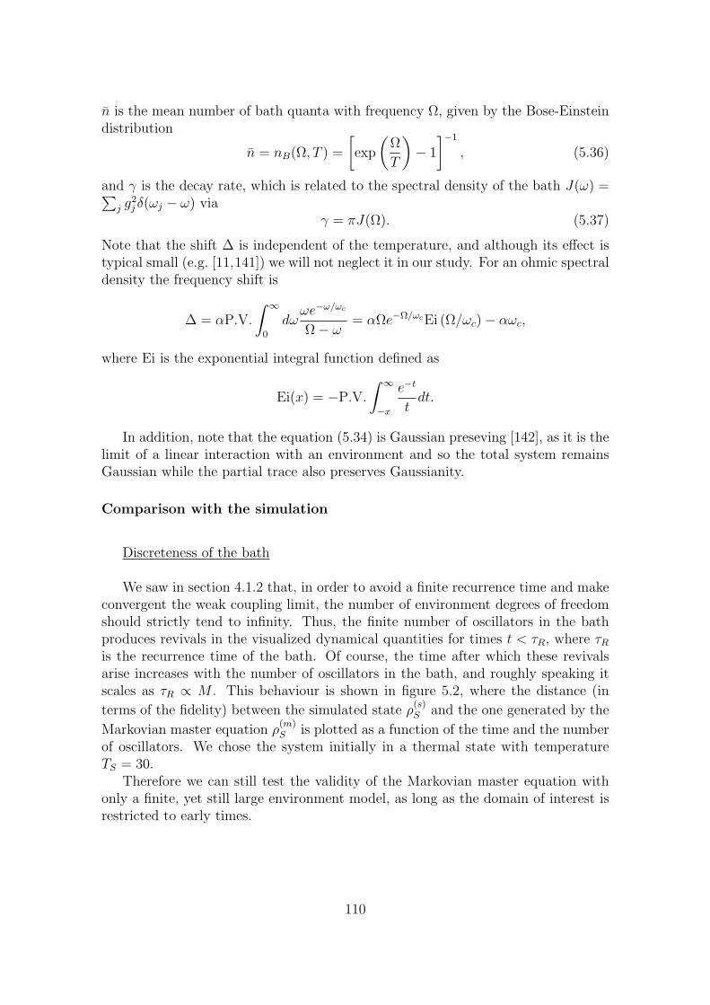
n is the mean number of bath quanta with frequency Ω, given by the Bose-Einsteindistribution
n = nB(Ω, T ) =
[exp
(Ω
T
)− 1
]−1
, (5.36)
and γ is the decay rate, which is related to the spectral density of the bath J(ω) =∑j g2
j δ(ωj − ω) viaγ = πJ(Ω). (5.37)
Note that the shift ∆ is independent of the temperature, and although its effect istypical small (e.g. [11,141]) we will not neglect it in our study. For an ohmic spectraldensity the frequency shift is
∆ = αP.V.
∫ ∞
0
dωωe−ω/ωc
Ω− ω= αΩe−Ω/ωcEi (Ω/ωc)− αωc,
where Ei is the exponential integral function defined as
Ei(x) = −P.V.
∫ ∞
−x
e−t
tdt.
In addition, note that the equation (5.34) is Gaussian preseving [142], as it is thelimit of a linear interaction with an environment and so the total system remainsGaussian while the partial trace also preserves Gaussianity.
Comparison with the simulation
Discreteness of the bath
We saw in section 4.1.2 that, in order to avoid a finite recurrence time and makeconvergent the weak coupling limit, the number of environment degrees of freedomshould strictly tend to infinity. Thus, the finite number of oscillators in the bathproduces revivals in the visualized dynamical quantities for times t < τR, where τR
is the recurrence time of the bath. Of course, the time after which these revivalsarise increases with the number of oscillators in the bath, and roughly speaking itscales as τR ∝ M . This behaviour is shown in figure 5.2, where the distance (in
terms of the fidelity) between the simulated state ρ(s)S and the one generated by the
Markovian master equation ρ(m)S is plotted as a function of the time and the number
of oscillators. We chose the system initially in a thermal state with temperatureTS = 30.
Therefore we can still test the validity of the Markovian master equation withonly a finite, yet still large environment model, as long as the domain of interest isrestricted to early times.
110
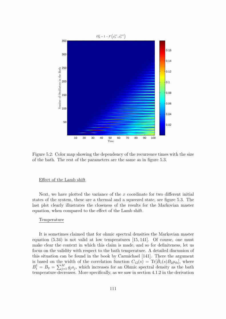
Time
D2B = 1 − F
(
ρ(s)S
, ρ(m)S
)
Num
ber
ofO
scilla
tors
inthe
Bath
10 20 30 40 50 60 70 80 90 100
50
100
150
200
250
300
350
0.02
0.04
0.06
0.08
0.1
0.12
0.14
0.16
Figure 5.2: Color map showing the dependency of the recurrence times with the sizeof the bath. The rest of the parameters are the same as in figure 5.3.
Effect of the Lamb shift
Next, we have plotted the variance of the x coordinate for two different initialstates of the system, these are a thermal and a squeezed state, see figure 5.3. Thelast plot clearly illustrates the closeness of the results for the Markovian masterequation, when compared to the effect of the Lamb shift.
Temperature
It is sometimes claimed that for ohmic spectral densities the Markovian masterequation (5.34) is not valid at low temperatures [15, 141]. Of course, one mustmake clear the context in which this claim is made, and so for definiteness, let usfocus on the validity with respect to the bath temperature. A detailed discussion ofthis situation can be found in the book by Carmichael [141]. There the argumentis based on the width of the correlation function C12(s) = Tr[B1(s)B2ρth], whereB†
1 = B2 =∑M
j=1 gjaj, which increases for an Ohmic spectral density as the bathtemperature decreases. More specifically, as we saw in section 4.1.2 in the derivation
111
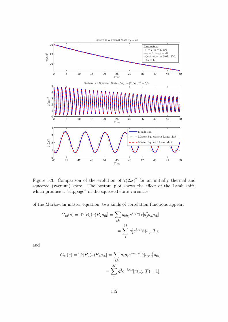
0 5 10 15 20 25 30 35 40 45 50
20
25
30
System in a Themal State TS = 30
Time
2(∆
x)2
0 5 10 15 20 25 30 35 40 45 500
1
2
3
4
5System in a Squeezed State (∆x)2 = [2(∆p)]−2 = 5/2
2(∆
x)2
Time
40 41 42 43 44 45 46 47 48 49 500
1
2
3
4
2(∆
x)2
Time
Simulation
Master Eq. without Lamb shift
Master Eq. with Lamb shift
Parameters:- Ω = 2, α = 1/500- ωc = 3, ωmax = 20,- Oscillators in Bath: 350,- TB = 1.
Figure 5.3: Comparison of the evolution of 2(∆x)2 for an initially thermal andsqueezed (vacuum) state. The bottom plot shows the effect of the Lamb shift,which produce a “slippage” in the squeezed state variances.
of the Markovian master equation, two kinds of correlation functions appear,
C12(s) = Tr[B1(s)B2ρth] =∑
j,k
gkgjeiωjsTr[a†jakρth]
=M∑j
g2j e
iωjsn(ωj, T ),
and
C21(s) = Tr[B2(s)B1ρth] =∑
j,k
gkgje−iωjsTr[aja
†kρth]
=M∑j
g2j e−iωjs[n(ωj, T ) + 1].
112
We may call C12(s) ≡ C(−s, T ) and C21(s) ≡ C(s, T ) + C0(s), and so in the contin-uous limit
C0(s) =
∫ ∞
0
J(ω)e−iωsdω = α
∫ ∞
0
ωe−iω(s−ω−1c )dω =
αω2c
(isωc + 1)2,
and
C(s, T ) =
∫ ∞
0
J(ω)e−iωsn(ω, T )dω = αT 2ζ
(2, 1− isT +
T
ωc
),
where here ζ(z, q) =∑∞
k=01
[(q+k)2]z/2 is the so-called Hurwitz Zeta function, which is
a generalization of the Riemann zeta function ζ(z) = ζ(z, 1) [143].
−50 0 500
0.02
0.04
0.06
0.08
0.1
0.12
s
|C(s
,T
)|
TB = 20TB = 10TB = 2
0 20 40 60 80 1000
5
10
15
20
25
TB
FW
HH
|C(s, T )||C0(s)|
50 60 70 80 90 1000.5
1
1.5
Figure 5.4: On the left, the absolute value of the correlation function is plotted forseveral temperatures while the FWHH as a function of temperature is representedon the right.
In the left plot of figure 5.4, the absolute value of C(s, T ) is plotted for differenttemperatures. Note that the spreading of the correlation function is mainly causedby its “height” decrease, that is, in the limit T → 0, C(s, T ) → 0. So one mayalso expect that the contribution of these correlations to the motion becomes lessimportant as T → 0, in such a way that the problem of the infinite width canbe counteracted, and this is indeed what seems to happen. To visualize this morecarefully we have plotted in the right of figure 5.4 the full weight at half height(FWHH) for both C0(s) and C(s, T ). Recall that in order to make valid the Marko-vian approximation, the typical time scale for the evolution of the system due toits interaction with the bath τS must be large in comparison with the decay timeτB of the correlation functions. Loosely speaking, this can be characterized by theFWHH.
From figure 5.4 one sees that for small temperatures τB (i.e. FWHH) is quitelarge, so it is expected that the Markovian approximation breaks down for values of
113
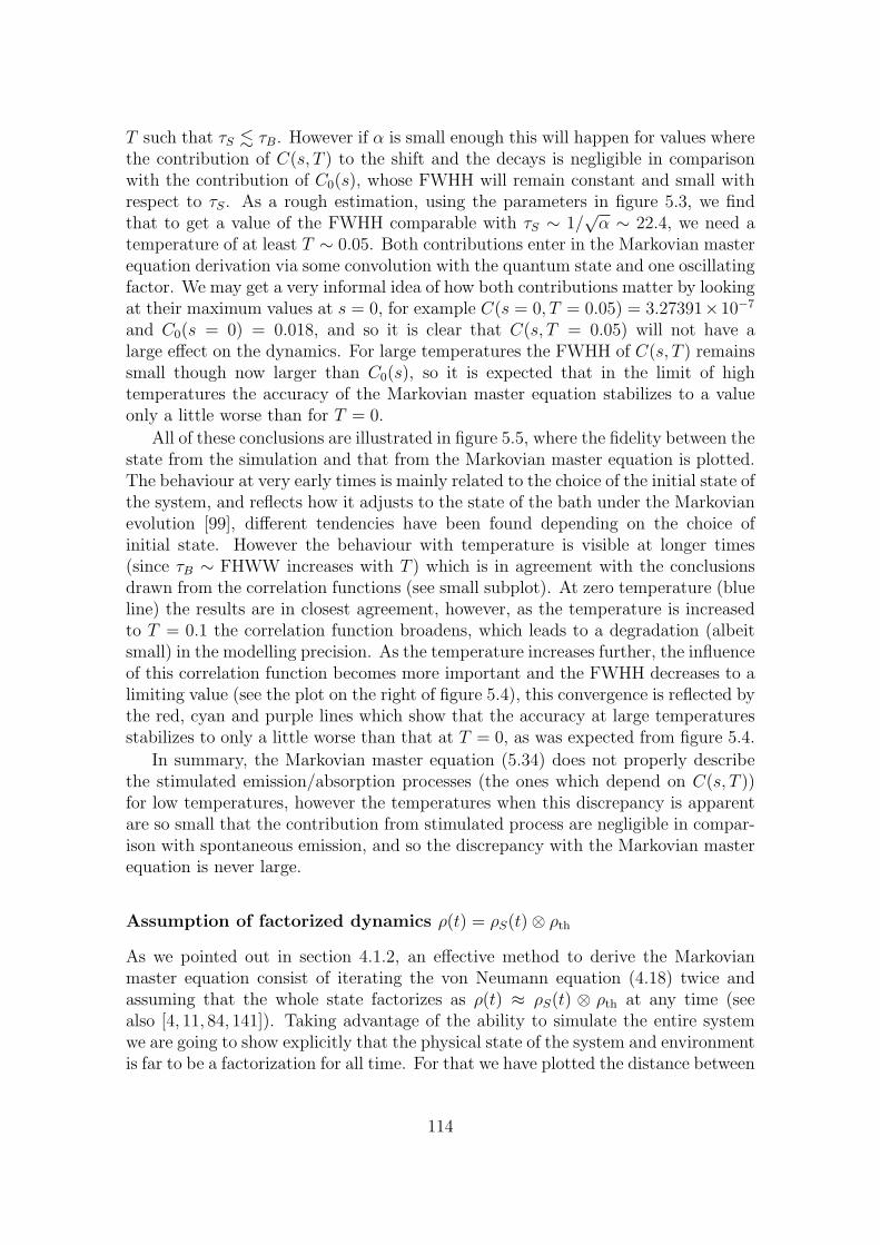
T such that τS . τB. However if α is small enough this will happen for values wherethe contribution of C(s, T ) to the shift and the decays is negligible in comparisonwith the contribution of C0(s), whose FWHH will remain constant and small withrespect to τS. As a rough estimation, using the parameters in figure 5.3, we findthat to get a value of the FWHH comparable with τS ∼ 1/
√α ∼ 22.4, we need a
temperature of at least T ∼ 0.05. Both contributions enter in the Markovian masterequation derivation via some convolution with the quantum state and one oscillatingfactor. We may get a very informal idea of how both contributions matter by lookingat their maximum values at s = 0, for example C(s = 0, T = 0.05) = 3.27391×10⁻⁷
and C0(s = 0) = 0.018, and so it is clear that C(s, T = 0.05) will not have alarge effect on the dynamics. For large temperatures the FWHH of C(s, T ) remainssmall though now larger than C0(s), so it is expected that in the limit of hightemperatures the accuracy of the Markovian master equation stabilizes to a valueonly a little worse than for T = 0.
All of these conclusions are illustrated in figure 5.5, where the fidelity between thestate from the simulation and that from the Markovian master equation is plotted.The behaviour at very early times is mainly related to the choice of the initial state ofthe system, and reflects how it adjusts to the state of the bath under the Markovianevolution [99], different tendencies have been found depending on the choice ofinitial state. However the behaviour with temperature is visible at longer times(since τB ∼ FHWW increases with T ) which is in agreement with the conclusionsdrawn from the correlation functions (see small subplot). At zero temperature (blueline) the results are in closest agreement, however, as the temperature is increasedto T = 0.1 the correlation function broadens, which leads to a degradation (albeitsmall) in the modelling precision. As the temperature increases further, the influenceof this correlation function becomes more important and the FWHH decreases to alimiting value (see the plot on the right of figure 5.4), this convergence is reflected bythe red, cyan and purple lines which show that the accuracy at large temperaturesstabilizes to only a little worse than that at T = 0, as was expected from figure 5.4.
In summary, the Markovian master equation (5.34) does not properly describethe stimulated emission/absorption processes (the ones which depend on C(s, T ))for low temperatures, however the temperatures when this discrepancy is apparentare so small that the contribution from stimulated process are negligible in compar-ison with spontaneous emission, and so the discrepancy with the Markovian masterequation is never large.
Assumption of factorized dynamics ρ(t) = ρS(t)⊗ ρth
As we pointed out in section 4.1.2, an effective method to derive the Markovianmaster equation consist of iterating the von Neumann equation (4.18) twice andassuming that the whole state factorizes as ρ(t) ≈ ρS(t) ⊗ ρth at any time (seealso [4, 11, 84, 141]). Taking advantage of the ability to simulate the entire systemwe are going to show explicitly that the physical state of the system and environmentis far to be a factorization for all time. For that we have plotted the distance between
114
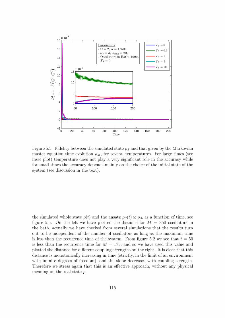
0 20 40 60 80 100 120 140 160 180 200−2
0
2
4
6
8
10
12
14
16
18x 10
−4
Time
D2 B
=1−
F(
ρ(s
)S
,ρ(m
)S
)
TB = 0
TB = 0.1
TB = 1
TB = 5
TB = 10
50 100 150 200
0
5
10
15x 10
−6
Parameters:
- Ω = 2, α = 1/500
- ωc = 3, ωmax = 20,
- Oscillators in Bath: 1000,
- TS = 0.
Figure 5.5: Fidelity between the simulated state ρS and that given by the Markovianmaster equation time evolution ρM , for several temperatures. For large times (seeinset plot) temperature does not play a very significant role in the accuracy whilefor small times the accuracy depends mainly on the choice of the initial state of thesystem (see discussion in the text).
the simulated whole state ρ(t) and the ansatz ρS(t)⊗ ρth as a function of time, seefigure 5.6. On the left we have plotted the distance for M = 350 oscillators inthe bath, actually we have checked from several simulations that the results turnout to be independent of the number of oscillators as long as the maximum timeis less than the recurrence time of the system. From figure 5.2 we see that t = 50is less than the recurrence time for M = 175, and so we have used this value andplotted the distance for different coupling strengths on the right. It is clear that thisdistance is monotonically increasing in time (strictly, in the limit of an environmentwith infinite degrees of freedom), and the slope decreases with coupling strength.Therefore we stress again that this is an effective approach, without any physicalmeaning on the real state ρ.
115
0 10 20 30 40 500
0.1
0.2
0.3
0.4
0.5
0.6
0.7
0.8
0.9
Time
DB
[
ρS(t
)⊗
ρth
,ρ(s
)]
0 10 20 30 40 500
0.1
0.2
0.3
0.4
0.5
0.6
0.7
0.8
0.9
Time
α = 10−3
α = 10−2
α = 10−1
Parameters:- Ω = 2, α = 1/500- ωc = 3, ωmax = 20,- Oscillators in Bath: 350,- TS = 1, TB = 30
Parameters:- Ω = 2- ωc = 3, ωmax = 20,- Oscillators in Bath: 175,- TS = 1, TB = 30
Figure 5.6: Distance between the simulated states ρS(t)⊗ ρth and ρ(t) as a functionof time; on the left side, different numbers of oscillators in the bath are plotted(obtaining the same result on that time scale), and on the right side, different valuesof the coupling constant have been taken.
5.2 Markovian master equations for interacting
systems
The damped harmonic oscillator is the canonical example used in most referencesto discuss both Markovian and non-Markovian open system dynamics (see for in-stance [4, 11, 13, 15, 80, 81, 141] and references therein) and exact solutions in thepresence of a general environment are known [124, 144]. However the dynamics ofcoupled damped oscillators, including those interacting with a semiclassical field, aresignificantly less studied, with most analysis focusing on evaluating the decoherenceof initially entangled states provided that certain dynamical evolution, Markovianor not, is valid [145]. Recently, an exact master equation for two interacting har-monic oscillators subject to a global general environment was derived [146]. In thissection we will focus on the derivation of Markovian master equations for interactingsystems.
We have extensively studied two damped systems. We start our analysis byanalyzing the dynamics of two interacting harmonic oscillators (section 5.2.1), find-ing Markovian master equations for both weak and strong internal coupling. Wefinally address the dynamics of an harmonic oscillator driven by a semiclassical field(section 5.2.2), where different Markovian master equations have been obtained andstudied depending on the values of the external Rabi frequency and the detuningfrom the oscillator’s natural frequency.
116
5.2.1 Two coupled damped harmonic oscillators
We now consider two coupled harmonic oscillators, which for simplicity we take tohave the same frequency Ω1 = Ω2 = Ω, and each locally damped by their ownreservoir (see figure 5.7), the Hamiltonian of the whole system is
H = H01 + H02 + V12 + HB1 + HB2 + V1B1 + V2B2, (5.38)
where the free Hamiltonians are given by
H01 = Ωa†1a1, H02 = Ωa†2a2,
HB1 =M∑
j=1
ω1ja†1ja1j, HB2 =
M∑j=1
ω2ja†2ja2j,
with the couplings to the baths,
V1B1 =M∑
j=1
g1j(a†1a1j + a1a
†1j),
V2B2 =M∑
j=1
g2j(a†2a2j + a2a
†2j),
and the coupling between oscillators,
V12 = β(a†1a2 + a1a†2).
As in the previous section we have employed here the rotating wave approximation,and so we assume Ω À β. For the case of Ω ∼ β we must keep the antirotatingterms a1a2 and a†1a
†2. However note that the eigenfrequencies of the normal modes
become imaginary if ω < 2β (see for example [147]) and the system then becomesunstable, so even when keeping the antirotating terms, we must limit β if we wishto keep the oscillatory behaviour.
Exact solution
For the exact solution, the extension to two oscillators follows closely that of a singledamped harmonic oscillator (see section 5.1.2). Again, we work in the Heisenbergpicture, and wish to solve for the vector A = (a1, a11, . . . , a1M , a2, a21, . . . , a2M)T,given the differential equation,
iA = WA, (5.39)
117
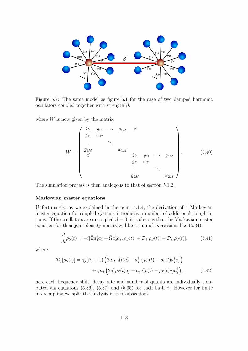
Figure 5.7: The same model as figure 5.1 for the case of two damped harmonicoscillators coupled together with strength β.
where W is now given by the matrix
W =
Ω1 g11 · · · g1M βg11 ω12...
. . .
g1M ω1M
β Ω2 g21 · · · g2M
g21 ω21...
. . .
g2M ω2M
. (5.40)
The simulation process is then analogous to that of section 5.1.2.
Markovian master equations
Unfortunately, as we explained in the point 4.1.4, the derivation of a Markovianmaster equation for coupled systems introduces a number of additional complica-tions. If the oscillators are uncoupled β = 0, it is obvious that the Markovian masterequation for their joint density matrix will be a sum of expressions like (5.34),
d
dtρS(t) = −i[Ωa†1a1 + Ωa†2a2, ρS(t)] +D1[ρS(t)] +D2[ρS(t)], (5.41)
where
Dj[ρS(t)] = γj(nj + 1)(2ajρS(t)a†j − a†jajρS(t)− ρS(t)a†jaj
)
+γjnj
(2a†jρS(t)aj − aja
†jρ(t)− ρS(t)aja
†j
), (5.42)
here each frequency shift, decay rate and number of quanta are individually com-puted via equations (5.36), (5.37) and (5.35) for each bath j. However for finiteintercoupling we split the analysis in two subsections.
118
Small intercoupling β
If β is sufficiently small to not affect the shift and decay rates, we deduced insection 4.1.4 that a Markovian master equation of the form
d
dtρS(t) = −i[Ωa†1a1 + Ωa†2a2 + V12, ρS(t)] +D1[ρS(t)] +D2[ρS(t)], (5.43)
will be a good description of the real dynamics. In addition, this kind of approxi-mation is often made in other contexts such as with damped systems driven by aclassical field [141]. Such a case will be analyzed in detail in section 5.2.2.
Large intercoupling β
To go further we must work in the interaction picture generated by the Hamil-tonian H0 = Hfree + V12 and apply the procedure of the weak coupling limit.
First, let us write the Hamiltonian of the two oscillator system in a more conve-nient way
H12 = H01 + H02 + V12 = (a†1, a†2)
(Ω1 ββ Ω2
)(a1
a2
).
We can diagonalize this quadratic form by means of a rotation to get
H12 = Ω+b†1b1 + Ω−b†2b2,
where
Ω± =(Ω1 + Ω2)±
√4β2 + (Ω1 − Ω2)2
2,
and the creation and annihilation operators in the rotated frame are given by
b1 = a1 cos(α)− a2 sin(α),
b2 = a1 sin(α) + a2 cos(α),
with the angle specified by
tan(α) =2β
(Ω1 − Ω2)−√
4β2 + (Ω1 − Ω2)2.
The new operators satisfy the standard bosonic commutation rules [bi, b†j] = δij, and
so this is nothing more than the decomposition of an oscillatory system in normalmodes. For simplicity, let us now take Ω1 = Ω2 = Ω, and so
Ω± = Ω± β,
b1 = 1√
2(a1 + a2)
b2 = 1√2(a1 − a2)
,
note that RWA approximation implies Ω À β so both normal mode frequencies arepositive.
119
We can reexpress the interactions with the baths in terms of these new operators,
V1B1 =M∑
j=1
g1j√2[(b†1 + b†2)a1j + (b1 + b2)a
†1j],
V2B2 =M∑
j=1
g2j√2[(b†1 − b†2)a2j + (b1 − b2)a
†2j],
the benefit of this is that it allows us to easily deal with the interaction picture withrespect to H0 = H12 + HB1 + HB2. In the weak coupling limit we obtain,
d
dtρS(t) = −
∫ ∞
0
dt′TrB1[V1B1(t), [V1B1(t− s), ρS(t)⊗ ρth1]]
−∫ ∞
0
dsTrB2[V2B2(t), [V2B2(t− s), ρS(t)⊗ ρth2]], (5.44)
where we have noted PV1B1V2B2P = PV2B2V1B1P = 0. Each of the above termscorrespond, essentially, to one of a pair of two free harmonic oscillators with fre-quencies Ω+ and Ω−, coupled to a common bath. Consequently, we can deal withthem separately. Starting with the first term
L1(ρS) = −∫ ∞
0
dsTrB1[V1B1(t), [V1B1(t− s), ρS(t− s)⊗ ρth1]], (5.45)
we decompose the interaction in to eigenoperators of [H12, ·] (see section 4.1.2)
V1B1 =∑
k
Ak ⊗Bk, (5.46)
with
A1 =1√2(b1 + b2), A2 =
1√2(b†1 + b†2),
B1 =M∑
j=1
g1ja†1j, B2 =
M∑j=1
g1ja1j. (5.47)
Notice the A1 operator can be written as A1 = A1(Ω+) + A1(Ω−), where A1(Ω+) =b1/√
2 and A1(Ω−) = b2/√
2 are already the eigenoperators of [H12, ·] with eigen-values −Ω+ and −Ω− respectively. Similarly A2 = A2(−Ω+) + A2(−Ω−), withA2(−Ω+) = b†1/
√2 and A2(−Ω−) = b†2/
√2, and so we can write (5.46) as
V1B1 =∑
k
Ak ⊗Bk =∑
ν,k
Ak(ν)⊗Bk =∑
ν,k
A†k(ν)⊗B†
k, (5.48)
which in interaction picture becomes
V1B1(t) =∑
ν,k
e−iνtAk(ν)⊗ Bk(t) =∑
ν,k
eiνtA†k(ν)⊗ B†
k(t).
120
Now, for the first element of Eq. (4.26) (in the limit s →∞), we have
Γ1,1(ν) =∑
j,j′g1jg1j′
∫ ∞
0
dsei(ν−ω1j)sTr(ρth
B1a1ja†1j′
)
=M∑
j=1
g21j
∫ ∞
0
dsei(ν−ω1j)s[n1(ω1j) + 1], (5.49)
where the mean number of quanta in the first bath n1(ω1j) with frequency ω1j,is given by the Bose-Einstein distribution (5.36). Going to the continuous limitwe take M → ∞ and introduce the spectral density of the first bath J1(ω) =∑
j g21jδ(ω − ω1j),
Γ1,1(ν) =
∫ ∞
0
dωJ1(ω)
∫ ∞
0
dsei(ν−ω)s[n1(ω) + 1].
Assuming ν > 0, we split into real and imaginary parts,
Γ1,1(ν) = γ1(ν)[n1(ν) + 1] + i[∆1(ν) + ∆′1(ν)],
where according to section 4.1.2
γ1(ν) = πJ1(ν),
∆1(ν) = P.V.
∫ ∞
0
dωJ1(ω)
ν − ω,
∆′1(ν) = P.V.
∫ ∞
0
dωJ1(ω)n1(ω)
ν − ω. (5.50)
Similar calculations give (ν > 0)
Γ1,2(−ν) = Γ2,1(ν) = 0, (5.51)
Γ2,2(−ν) = γ1(ν)n1(ν)− i∆′1(ν). (5.52)
Thus, equation (5.45) becomes
L1(ρS) =∑
ν,ν′ei(ν′−ν)tΓ1,1(ν)[A1(ν)ρS(t), A†
1(ν′)]
+ ei(ν−ν′)tΓ∗1,1(ν)[A1(ν′), ρS(t)A†
1(ν)]
+ ei(ν′−ν)tΓ2,2(ν)[A2(ν)ρS(t), A†2(ν
′)]
+ ei(ν−ν′)tΓ∗2,2(ν)[A2(ν′), ρS(t)A†
2(ν)]. (5.53)
Next we perform the secular approximation; the cross terms ν ′ 6= ν in the above ex-pression, which go as e±2βti, can be neglected provided that 2β is large in comparison
121
with the inverse of the relaxation rate (β À α) and so we obtain
L1(ρS) = − i∆1(Ω+)
2[b†1b1, ρS(t)]− i
∆1(Ω−)
2[b†2b2, ρS(t)]
+ γ1(Ω+)[n1(Ω+) + 1]
(b1ρS(t)b†1 −
1
2b†1b1, ρS(t)
)
+ γ1(Ω+)n1(Ω+)
(b†1ρS(t)b1 − 1
2b1b
†1, ρS(t)
)
+ γ1(Ω−)[n1(Ω−) + 1]
(b2ρS(t)b†2 −
1
2b†2b2, ρS(t)
)
+ γ1(Ω−)n1(Ω−)
(b†2ρS(t)b2 − 1
2b2b
†2, ρS(t)
). (5.54)
Returning to equation (5.44), for the second term,
L2(ρS) = −∫ ∞
0
dsTrB1[V2B2(t), [V2B2(t− s), ρS(t)⊗ ρth2]],
the situation is essentially the same, since the minus sign in b2 only modifies the crossterms, which we neglect in the secular approximation. Following similar steps as inthe above we obtain the same form (5.54) for L2, with the replacements γ1 → γ2,∆1 → ∆2 and n1 → n2, where the subscript 2 refers to the corresponding expressionwith the spectral density and temperature of the second bath. Therefore puttingtogether both quantities, and returning to the Schrodinger picture
d
dtρS(t) = − i [Ω1 + ∆1(Ω+)/2 + ∆2(Ω+)/2] [b†1b1, ρS(t)]
− i [Ω2 + ∆1(Ω−)/2 + ∆2(Ω−)/2] [b†2b2, ρS(t)]
+ γ1(Ω+)[n1(Ω+) + 1]
+ γ2(Ω+)[n2(Ω+) + 1](
b1ρS(t)b†1 −1
2b†1b1, ρS(t)
)
+ [γ1(Ω+)n1(Ω+) + γ2(Ω+)n2(Ω+)]
(b†1ρS(t)b1 − 1
2b1b
†1, ρS(t)
)
+ γ1(Ω−)[n1(Ω−) + 1]
+ γ2(Ω−)[n2(Ω−) + 1](
b2ρS(t)b†2 −1
2b†2b2, ρS(t)
)
+ [γ1(Ω−)n1(Ω−) + γ2(Ω−)n2(Ω−)]
(b†2ρS(t)b2 − 1
2b2b
†2, ρS(t)
).
It is manifestly clear that this equation is of the Kossakowski-Lindblad form. Finally,we rewrite the operators b1 and b2 in terms of a1 and a2 to arrive at
122
d
dtρS(t) = −i[Ωa†1a1 + Ωa†2a2 + β
(a1a
†2 + a†1a2
), ρS(t)]
+2∑
j,k
K(E)jk
[ajρS(t)a†k +
1
2a†kaj, ρS(t)
]
+2∑
j,k
K(A)jk
[a†jρS(t)ak +
1
2aka
†j, ρS(t)
], (5.55)
here
Ω = Ω + [∆1(Ω+) + ∆2(Ω+) + ∆1(Ω−) + ∆2(Ω−)]/4,
β = β + [∆1(Ω+) + ∆2(Ω+)−∆1(Ω−)−∆2(Ω−)]/4,
and K(E)jk and K
(A)jk are two positive semidefinite Hermitian matrices with coefficients
K(E)11 = K
(E)22 = γ1(Ω+)[n1(Ω+) + 1] + γ2(Ω+)[n2(Ω+) + 1]
+ γ1(Ω−)[n1(Ω−) + 1] + γ2(Ω−)[n2(Ω−) + 1]/2, (5.56)
K(E)12 = K
(E)∗21 = γ1(Ω+)[n1(Ω+) + 1] + γ2(Ω+)[n2(Ω+) + 1]
− γ1(Ω−)[n1(Ω−) + 1]− γ2(Ω−)[n2(Ω−) + 1]/2, (5.57)
K(A)11 = K
(A)22 = [γ1(Ω+)n1(Ω+) + γ2(Ω+)n2(Ω+)
+ γ1(Ω−)n1(Ω−) + γ2(Ω−)n2(Ω−)]/2, (5.58)
K(A)12 = K
(A)∗21 = [γ1(Ω+)n1(Ω+) + γ2(Ω+)n2(Ω+)
− γ1(Ω−)n1(Ω−)− γ2(Ω−)n2(Ω−)]/2, (5.59)
where γj, ∆j and nj are evaluated according to the spectral density and temperatureof the bath j and Ω± = Ω± β.
Note that in order to neglect the non-secular terms which oscillate with a phasee±2iβt, we must impose β À α, therefore the resultant equation is, in some sense,complementary to (5.43) valid if α & β.
It is worth mentioning that similar equations for coupled harmonic oscillatorshave been given previously (see for example [148,149]), but not in the Kossakowski-Lindblad form, since in those derivations the secular approximation is not taken.
Comparison with the simulation
By virtue of the derivation, equations (5.43) and (5.55) preserve both completepositivity and Gaussianity (because they arise from a linear interaction with theenvironment). Thus we can test their regimes of validity using simulations of Gaus-sian states, and the appropriate fidelity formulas. In figure 5.8 we have plotted the
123
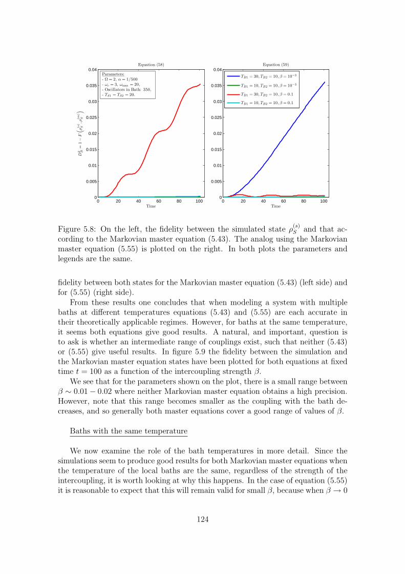
0 20 40 60 80 1000
0.005
0.01
0.015
0.02
0.025
0.03
0.035
0.04Equation (58)
Time
D2 B
=1−
F(
ρ(s
)S
,ρ(m
)S
)
1
0 20 40 60 80 1000
0.005
0.01
0.015
0.02
0.025
0.03
0.035
0.04
Time
Equation (59)
TB1 = 30, TB2 = 10, β = 10−3
TB1 = 10, TB2 = 10, β = 10−3
TB1 = 30, TB2 = 10, β = 0.1
TB1 = 10, TB2 = 10, β = 0.1
Parameters:- Ω = 2, α = 1/500- ωc = 3, ωmax = 20,- Oscillators in Bath: 350,- TS1 = TS2 = 20.
Figure 5.8: On the left, the fidelity between the simulated state ρ(s)S and that ac-
cording to the Markovian master equation (5.43). The analog using the Markovianmaster equation (5.55) is plotted on the right. In both plots the parameters andlegends are the same.
fidelity between both states for the Markovian master equation (5.43) (left side) andfor (5.55) (right side).
From these results one concludes that when modeling a system with multiplebaths at different temperatures equations (5.43) and (5.55) are each accurate intheir theoretically applicable regimes. However, for baths at the same temperature,it seems both equations give good results. A natural, and important, question isto ask is whether an intermediate range of couplings exist, such that neither (5.43)or (5.55) give useful results. In figure 5.9 the fidelity between the simulation andthe Markovian master equation states have been plotted for both equations at fixedtime t = 100 as a function of the intercoupling strength β.
We see that for the parameters shown on the plot, there is a small range betweenβ ∼ 0.01− 0.02 where neither Markovian master equation obtains a high precision.However, note that this range becomes smaller as the coupling with the bath de-creases, and so generally both master equations cover a good range of values of β.
Baths with the same temperature
We now examine the role of the bath temperatures in more detail. Since thesimulations seem to produce good results for both Markovian master equations whenthe temperature of the local baths are the same, regardless of the strength of theintercoupling, it is worth looking at why this happens. In the case of equation (5.55)it is reasonable to expect that this will remain valid for small β, because when β → 0
124
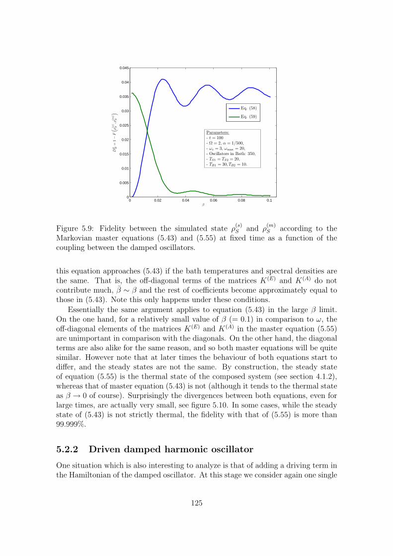
0 0.02 0.04 0.06 0.08 0.10
0.005
0.01
0.015
0.02
0.025
0.03
0.035
0.04
0.045
β
D2 B
=1−
F(
ρ(s
)S
,ρ(m
)S
)
Eq. (58)
Eq. (59)
Parameters:- t = 100- Ω = 2, α = 1/500,- ωc = 3, ωmax = 20,- Oscillators in Bath: 350,- TS1 = TS2 = 20,- TB1 = 30, TB2 = 10.
Figure 5.9: Fidelity between the simulated state ρ(s)S and ρ
(m)S according to the
Markovian master equations (5.43) and (5.55) at fixed time as a function of thecoupling between the damped oscillators.
this equation approaches (5.43) if the bath temperatures and spectral densities arethe same. That is, the off-diagonal terms of the matrices K(E) and K(A) do notcontribute much, β ∼ β and the rest of coefficients become approximately equal tothose in (5.43). Note this only happens under these conditions.
Essentially the same argument applies to equation (5.43) in the large β limit.On the one hand, for a relatively small value of β (= 0.1) in comparison to ω, theoff-diagonal elements of the matrices K(E) and K(A) in the master equation (5.55)are unimportant in comparison with the diagonals. On the other hand, the diagonalterms are also alike for the same reason, and so both master equations will be quitesimilar. However note that at later times the behaviour of both equations start todiffer, and the steady states are not the same. By construction, the steady stateof equation (5.55) is the thermal state of the composed system (see section 4.1.2),whereas that of master equation (5.43) is not (although it tends to the thermal stateas β → 0 of course). Surprisingly the divergences between both equations, even forlarge times, are actually very small, see figure 5.10. In some cases, while the steadystate of (5.43) is not strictly thermal, the fidelity with that of (5.55) is more than99.999%.
5.2.2 Driven damped harmonic oscillator
One situation which is also interesting to analyze is that of adding a driving term inthe Hamiltonian of the damped oscillator. At this stage we consider again one single
125
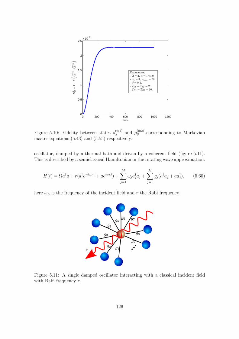
0 200 400 600 800 1000 12000
0.5
1
1.5
2
2.5x 10
−6
Time
D2 B
=1−
F(
ρ(m
1)
S,ρ
(m2)
S
)
Parameters:
- Ω = 2, α = 1/500
- ωc = 3, ωmax = 20,
- β = 0.1,
- TS1 = TS2 = 20.
- TB1 = TB2 = 10.
Figure 5.10: Fidelity between states ρ(m1)S and ρ
(m2)S corresponding to Markovian
master equations (5.43) and (5.55) respectively.
oscillator, damped by a thermal bath and driven by a coherent field (figure 5.11).This is described by a semiclassical Hamiltonian in the rotating wave approximation:
H(t) = Ωa†a + r(a†e−iωLt + aeiωLt) +M∑
j=1
ωja†jaj +
M∑j=1
gj(a†aj + aa†j), (5.60)
here ωL is the frequency of the incident field and r the Rabi frequency.
Figure 5.11: A single damped oscillator interacting with a classical incident fieldwith Rabi frequency r.
126
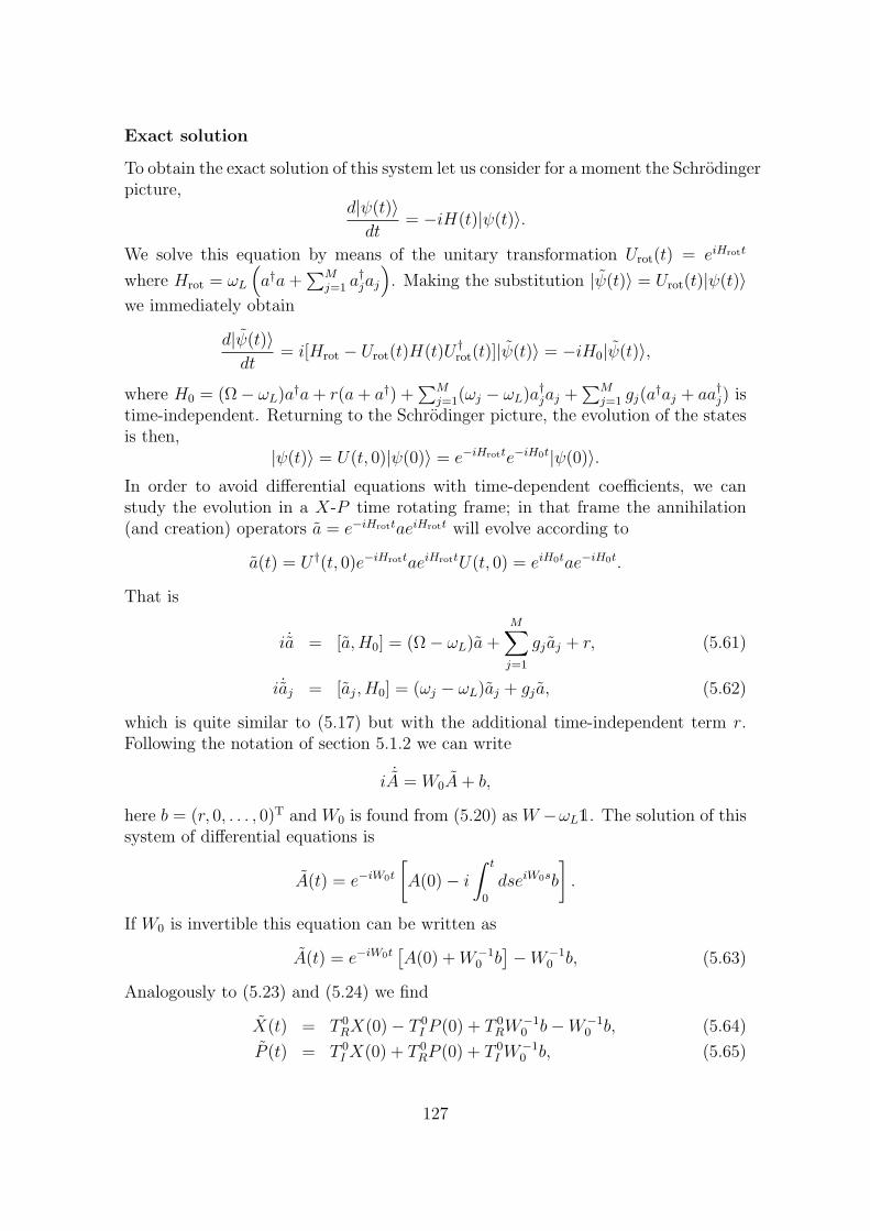
Exact solution
To obtain the exact solution of this system let us consider for a moment the Schrodingerpicture,
d|ψ(t)〉dt
= −iH(t)|ψ(t)〉.We solve this equation by means of the unitary transformation Urot(t) = eiHrott
where Hrot = ωL
(a†a +
∑Mj=1 a†jaj
). Making the substitution |ψ(t)〉 = Urot(t)|ψ(t)〉
we immediately obtain
d|ψ(t)〉dt
= i[Hrot − Urot(t)H(t)U †rot(t)]|ψ(t)〉 = −iH0|ψ(t)〉,
where H0 = (Ω− ωL)a†a + r(a + a†) +∑M
j=1(ωj − ωL)a†jaj +∑M
j=1 gj(a†aj + aa†j) is
time-independent. Returning to the Schrodinger picture, the evolution of the statesis then,
|ψ(t)〉 = U(t, 0)|ψ(0)〉 = e−iHrotte−iH0t|ψ(0)〉.In order to avoid differential equations with time-dependent coefficients, we canstudy the evolution in a X-P time rotating frame; in that frame the annihilation(and creation) operators a = e−iHrottaeiHrott will evolve according to
a(t) = U †(t, 0)e−iHrottaeiHrottU(t, 0) = eiH0tae−iH0t.
That is
i ˙a = [a, H0] = (Ω− ωL)a +M∑
j=1
gj aj + r, (5.61)
i ˙aj = [aj, H0] = (ωj − ωL)aj + gj a, (5.62)
which is quite similar to (5.17) but with the additional time-independent term r.Following the notation of section 5.1.2 we can write
i ˙A = W0A + b,
here b = (r, 0, . . . , 0)T and W0 is found from (5.20) as W −ωL1. The solution of thissystem of differential equations is
A(t) = e−iW0t
[A(0)− i
∫ t
0
dseiW0sb
].
If W0 is invertible this equation can be written as
A(t) = e−iW0t[A(0) + W−1
0 b]−W−1
0 b, (5.63)
Analogously to (5.23) and (5.24) we find
X(t) = T 0RX(0)− T 0
I P (0) + T 0RW−1
0 b−W−10 b, (5.64)
P (t) = T 0I X(0) + T 0
RP (0) + T 0I W−1
0 b, (5.65)
127
where T 0R and T 0
I are as in (5.25) for W0. Thus, by writing
M0 =
(T 0
R −T 0I
T 0I T 0
R
), B =
((T 0
R − 1)W−10 b
T 0I W−1
0 b
),
we find that the position and momentum expectation values evolve as
R(t) = M0R(0) + B. (5.66)
Note that in this case the first moments of the state change, despite 〈R(0)〉 = 0.To calculate the evolution of the covariance matrix, we proceed in the same way asbefore,
〈Ri(t)Rj(t)〉 =∑
k,`
M0i,kM0
j,`〈Ri(0)Rj(0)〉+∑
k
M0i,k〈Rk(0)〉Bj
+Bj
∑
k
M0j,`〈R`(0)〉+ BiBj, (5.67)
and analogously for the solutions for 〈Rj(t)Ri(t)〉 and 〈Ri(t)〉〈Rj(t)〉. Combiningthese terms, we find the B cancel and so, in a similar fashion to (5.29),(5.30) and(5.31),
C1,1(t) = (M01, C(0)M0
1),
C1,M+2(t) = CM+2,1(t) = (M01, CM0
M+2)
CM+2,M+2(t) = (M0M+2, CM0
M+2), (5.68)
where, of course, M01 and M0
2 are as in (5.33) for M0.
Markovian master equations
Following the method explained in section 4.1.4 we will be able to obtain Markovianmaster equations valid for large (to some degree) Rabi frequencies, even thoughthe complexity of the problem has increased. In our derivation, we will distinguishbetween three cases: these will be when the Rabi frequency is very small; when thedriving is far off resonance (|ωL−Ω| À 0) and finally the identical case without thesecular approximation.
In these three cases we find a Markovian master equation with the structure
d
dtρS = −i[Ωa†a + reiωLta + r∗e−iωLta†, ρS] +D(ρS),
where D is given by (5.42) (for one oscillator), Ω = Ω+∆ is the same as for a singledamped oscillator, and r is a renormalized Rabi frequency due to the effect of thebath. Note that as the incident field alters the position operator of the oscillator,which in turn couples to the bath, one should expect that the field is itself also
128
affected by the environment. For small Rabi frequencies an argument similar tosection 5.2.1 gives simply
r = r, (5.69)
whereas, when the driving field is far from resonance, |ωL − Ω| À 0, we obtain
r = r
[1 +
∆(Ω) + iγ(Ω)
Ω− ωL
]. (5.70)
Finally, if we do not make the secular approximation, the renormalized Rabi fre-quency yields
r = r
[1 +
∆(Ω) + iγ(Ω)
Ω− ωL
− ∆(ωL) + iγ(ωL)
Ω− ωL
]. (5.71)
To derive a completely positive Markovian master equation valid for large Rabifrequencies r we work in the interaction picture generated by the unitary propagator
U(t1, t0) = T e−i∫ t1
t0H1(t′)dt′ , where
H1(t) = Ωa†a + r(a†e−iωLt + aeiωLt) +M∑
j=1
ωja†jaj. (5.72)
Taking t0 = 0 without lost of generality, the time-evolution equation for ρ(t) =U †(t, 0)ρ(t)U(t, 0) is
˙ρ(t) = −i[V (t), ρ(t)], (5.73)
so by following the analogous procedure for time-independent generators, to getsomething similar to the eigenoperator decomposition for V (t) = U †(t, 0)V U(t, 0)(V =
∑Mj=1 gj(a
†aj + aa†j)). We note that the operator A1(t) = a(t) satisfies adifferential equation with periodic terms
i ˙a(t) = [a(t), H0(t)] = Ωa(t) + re−iωLt. (5.74)
Thus, provided that its solution is also periodic Ak(t) =∑
ν Ak(ν)eiνt (see section4.1.4) there is not further problem in the derivation. Note once more that theimportance of such a decomposition is that the operators Ak(ν) are themselvestime-independent.
The solution to equation (5.74), with the initial condition a(0) = a and forΩ 6= ωL is given by
a(t) =r(e−iωLt − e−iΩt) + a(ωL − Ω)e−iΩt
ωL − Ω, (5.75)
so in this case the solution is periodic and the desired decomposition A1(t) =∑ν A1(ν)eiνt is
A1(t) = A1(ωL)e−iωLt + A2(Ω)e−iΩt,
where A1(ωL) = rωL−Ω
1 and A1(Ω) = a− rωL−Ω
1 = a− A1(ωL). Similarly
A2(t) = A2(−ωL)eiωLt + A2(−Ω)eiΩt,
129
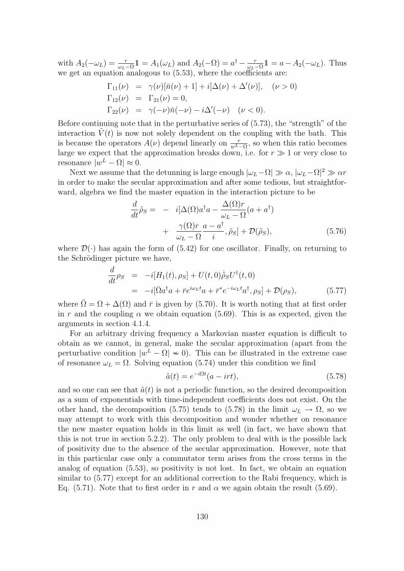
with A2(−ωL) = rωL−Ω
1 = A1(ωL) and A2(−Ω) = a†− rωL−Ω
1 = a−A2(−ωL). Thuswe get an equation analogous to (5.53), where the coefficients are:
Γ11(ν) = γ(ν)[n(ν) + 1] + i[∆(ν) + ∆′(ν)], (ν > 0)
Γ12(ν) = Γ21(ν) = 0,
Γ22(ν) = γ(−ν)n(−ν)− i∆′(−ν) (ν < 0).
Before continuing note that in the perturbative series of (5.73), the “strength” of theinteraction V (t) is now not solely dependent on the coupling with the bath. Thisis because the operators A(ν) depend linearly on r
wL−Ω, so when this ratio becomes
large we expect that the approximation breaks down, i.e. for r À 1 or very close toresonance |wL − Ω| ≈ 0.
Next we assume that the detunning is large enough |ωL−Ω| À α, |ωL−Ω|2 À αrin order to make the secular approximation and after some tedious, but straightfor-ward, algebra we find the master equation in the interaction picture to be
d
dtρS = − i[∆(Ω)a†a− ∆(Ω)r
ωL − Ω(a + a†)
+γ(Ω)r
ωL − Ω
a− a†
i, ρS] +D(ρS), (5.76)
where D(·) has again the form of (5.42) for one oscillator. Finally, on returning tothe Schrodinger picture we have,
d
dtρS = −i[H1(t), ρS] + U(t, 0) ˙ρSU †(t, 0)
= −i[Ωa†a + reiωLta + r∗e−iωLta†, ρS] +D(ρS), (5.77)
where Ω = Ω + ∆(Ω) and r is given by (5.70). It is worth noting that at first orderin r and the coupling α we obtain equation (5.69). This is as expected, given thearguments in section 4.1.4.
For an arbitrary driving frequency a Markovian master equation is difficult toobtain as we cannot, in general, make the secular approximation (apart from theperturbative condition |wL − Ω| 0). This can be illustrated in the extreme caseof resonance ωL = Ω. Solving equation (5.74) under this condition we find
a(t) = e−iΩt(a− irt), (5.78)
and so one can see that a(t) is not a periodic function, so the desired decompositionas a sum of exponentials with time-independent coefficients does not exist. On theother hand, the decomposition (5.75) tends to (5.78) in the limit ωL → Ω, so wemay attempt to work with this decomposition and wonder whether on resonancethe new master equation holds in this limit as well (in fact, we have shown thatthis is not true in section 5.2.2). The only problem to deal with is the possible lackof positivity due to the absence of the secular approximation. However, note thatin this particular case only a commutator term arises from the cross terms in theanalog of equation (5.53), so positivity is not lost. In fact, we obtain an equationsimilar to (5.77) except for an additional correction to the Rabi frequency, which isEq. (5.71). Note that to first order in r and α we again obtain the result (5.69).
130
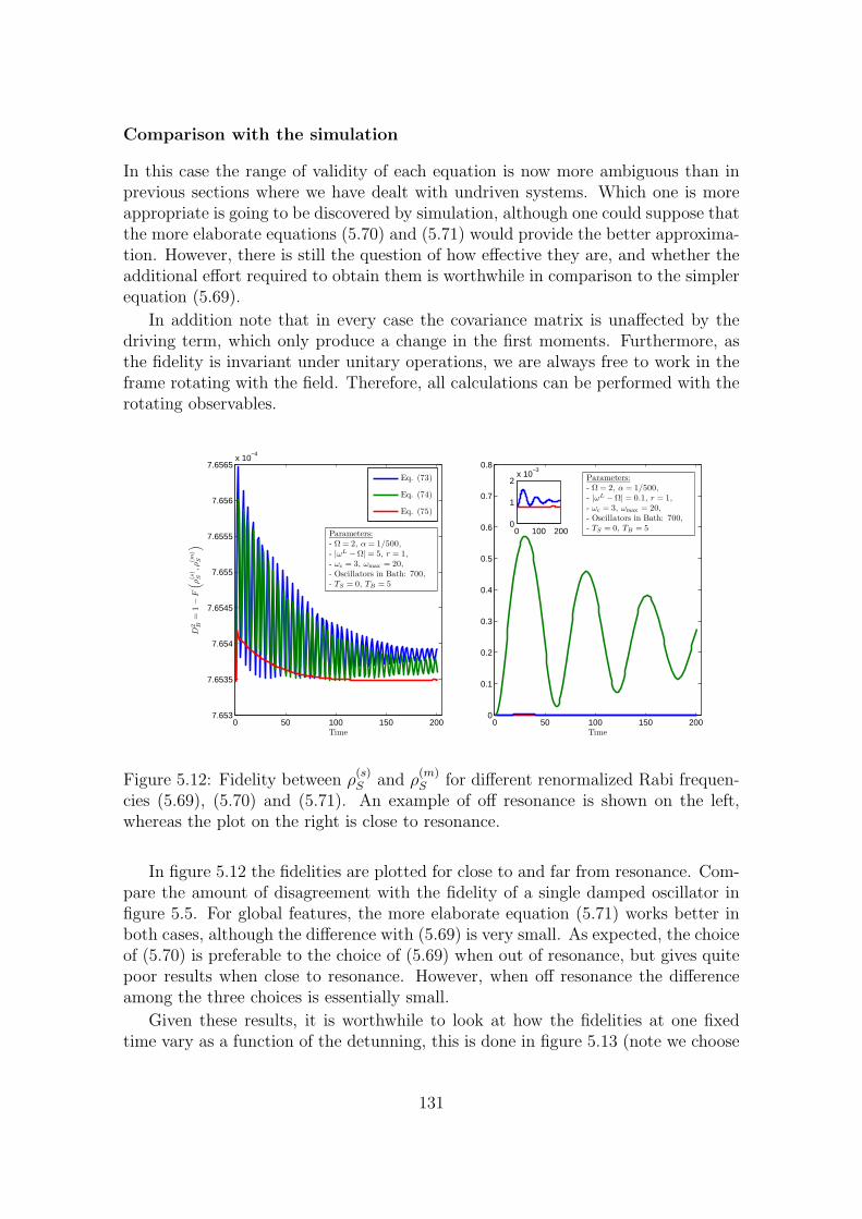
Comparison with the simulation
In this case the range of validity of each equation is now more ambiguous than inprevious sections where we have dealt with undriven systems. Which one is moreappropriate is going to be discovered by simulation, although one could suppose thatthe more elaborate equations (5.70) and (5.71) would provide the better approxima-tion. However, there is still the question of how effective they are, and whether theadditional effort required to obtain them is worthwhile in comparison to the simplerequation (5.69).
In addition note that in every case the covariance matrix is unaffected by thedriving term, which only produce a change in the first moments. Furthermore, asthe fidelity is invariant under unitary operations, we are always free to work in theframe rotating with the field. Therefore, all calculations can be performed with therotating observables.
0 50 100 150 2007.653
7.6535
7.654
7.6545
7.655
7.6555
7.656
7.6565x 10
−4
Time
D2 B
=1−
F(
ρ(s
)S
,ρ(m
)S
)
1
Eq. (73)
Eq. (74)
Eq. (75)
0 50 100 150 2000
0.1
0.2
0.3
0.4
0.5
0.6
0.7
0.8
Time
0 100 2000
1
2x 10
−3
Parameters:- Ω = 2, α = 1/500,- |ωL −Ω| = 0.1, r = 1,- ωc = 3, ωmax = 20,- Oscillators in Bath: 700,- TS = 0, TB = 5
Parameters:- Ω = 2, α = 1/500,- |ωL −Ω| = 5, r = 1,- ωc = 3, ωmax = 20,- Oscillators in Bath: 700,- TS = 0, TB = 5
Figure 5.12: Fidelity between ρ(s)S and ρ
(m)S for different renormalized Rabi frequen-
cies (5.69), (5.70) and (5.71). An example of off resonance is shown on the left,whereas the plot on the right is close to resonance.
In figure 5.12 the fidelities are plotted for close to and far from resonance. Com-pare the amount of disagreement with the fidelity of a single damped oscillator infigure 5.5. For global features, the more elaborate equation (5.71) works better inboth cases, although the difference with (5.69) is very small. As expected, the choiceof (5.70) is preferable to the choice of (5.69) when out of resonance, but gives quitepoor results when close to resonance. However, when off resonance the differenceamong the three choices is essentially small.
Given these results, it is worthwhile to look at how the fidelities at one fixedtime vary as a function of the detunning, this is done in figure 5.13 (note we choose
131
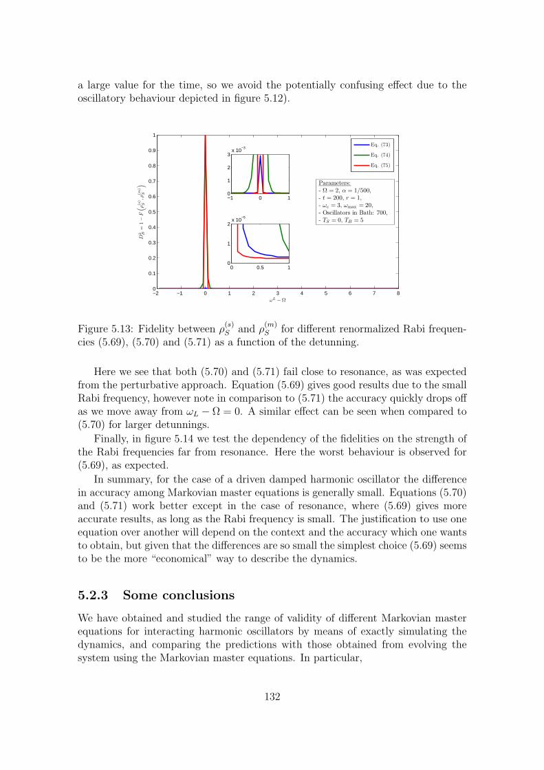
a large value for the time, so we avoid the potentially confusing effect due to theoscillatory behaviour depicted in figure 5.12).
−2 −1 0 1 2 3 4 5 6 7 80
0.1
0.2
0.3
0.4
0.5
0.6
0.7
0.8
0.9
1
ωL−Ω
D2 B
=1−
F(
ρ(s
)S
,ρ(m
)S
)
−1 0 10
1
2
3x 10
−3
0 0.5 10
1
2x 10
−5
Eq. (73)
Eq. (74)
Eq. (75)
Parameters:- Ω = 2, α = 1/500,- t = 200, r = 1,- ωc = 3, ωmax = 20,- Oscillators in Bath: 700,- TS = 0, TB = 5
Figure 5.13: Fidelity between ρ(s)S and ρ
(m)S for different renormalized Rabi frequen-
cies (5.69), (5.70) and (5.71) as a function of the detunning.
Here we see that both (5.70) and (5.71) fail close to resonance, as was expectedfrom the perturbative approach. Equation (5.69) gives good results due to the smallRabi frequency, however note in comparison to (5.71) the accuracy quickly drops offas we move away from ωL − Ω = 0. A similar effect can be seen when compared to(5.70) for larger detunnings.
Finally, in figure 5.14 we test the dependency of the fidelities on the strength ofthe Rabi frequencies far from resonance. Here the worst behaviour is observed for(5.69), as expected.
In summary, for the case of a driven damped harmonic oscillator the differencein accuracy among Markovian master equations is generally small. Equations (5.70)and (5.71) work better except in the case of resonance, where (5.69) gives moreaccurate results, as long as the Rabi frequency is small. The justification to use oneequation over another will depend on the context and the accuracy which one wantsto obtain, but given that the differences are so small the simplest choice (5.69) seemsto be the more “economical” way to describe the dynamics.
5.2.3 Some conclusions
We have obtained and studied the range of validity of different Markovian masterequations for interacting harmonic oscillators by means of exactly simulating thedynamics, and comparing the predictions with those obtained from evolving thesystem using the Markovian master equations. In particular,
132
0 10 20 30 40 50 60 70 80 90 1000
0.2
0.4
0.6
0.8
1
1.2x 10
−4
r
D2 B
=1−
F(
ρ(s
)S
,ρ(m
)S
)
Eq. (73)
Eq. (74)
Eq. (75)
Parameters:- Ω = 2, α = 1/500,- |ωL −Ω| = 5, t = 200,- ωc = 3, ωmax = 20,- Oscillators in Bath: 700,- TS = 0, TB = 5
Figure 5.14: Fidelity between ρ(s)S and ρ
(m)S for different renormalized Rabi frequen-
cies (5.69), (5.70) and (5.71) as a function of the Rabi frequency.
• We analysed two strategies for finding completely positive Markovian masterequations for two harmonic oscillators coupled together under the effect oflocal baths, indicating that both are complementary in their range of validity.Moreover, when the temperature of the local baths is the same the differencebetween them is quite small.
• In the same spirit, we derived time inhomogeneous completely positive Marko-vian master equations for a damped oscillator which is driven by an externalsemi-classical field. We studied the validity of each one and pointed out thatcompletely positive dynamics can be obtained even without secular approxi-mation (for these kinds of inhomogeneous equations).
Despite the fact that we have focused on harmonic oscillator systems, the proposedmethod is general and we expect that non-harmonic systems should behave in asimilar manner with respect to the validity of the equations. This suggest that thegeneral conclusions made here are widely applicable to any other settings involvinga weak interaction with an environment.
In this regard, we hope that the present results may help in providing a betterunderstanding and a transparent description of noise in interacting systems, includ-ing those situations where the strength of the internal system interaction is large.There are currently many quantum scenarios open to the use of these techniques, in-cluding realizations of harmonic and spin chains in systems of trapped ions [150,151],superconducting qubits [152] and nitrogen-vacancy (NV) defects in diamond [153].
Moreover, interacting systems subject to local reservoirs have been recentlytreated under the assumption of weak internal system interaction in theoretical
133

studies ranging from the excitation transport properties of biomolecules [154–159]to the stability of topological codes for quantum information [160–162].
134
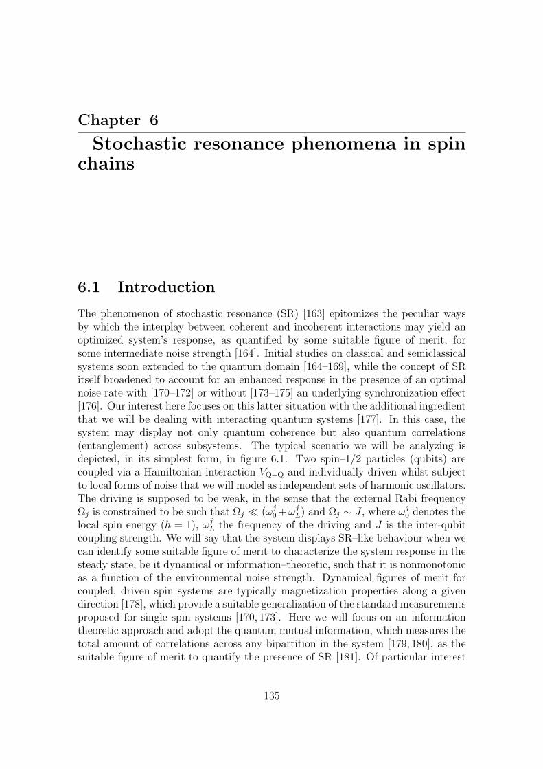
Chapter 6
Stochastic resonance phenomena in spinchains
6.1 Introduction
The phenomenon of stochastic resonance (SR) [163] epitomizes the peculiar waysby which the interplay between coherent and incoherent interactions may yield anoptimized system’s response, as quantified by some suitable figure of merit, forsome intermediate noise strength [164]. Initial studies on classical and semiclassicalsystems soon extended to the quantum domain [164–169], while the concept of SRitself broadened to account for an enhanced response in the presence of an optimalnoise rate with [170–172] or without [173–175] an underlying synchronization effect[176]. Our interest here focuses on this latter situation with the additional ingredientthat we will be dealing with interacting quantum systems [177]. In this case, thesystem may display not only quantum coherence but also quantum correlations(entanglement) across subsystems. The typical scenario we will be analyzing isdepicted, in its simplest form, in figure 6.1. Two spin–1/2 particles (qubits) arecoupled via a Hamiltonian interaction VQ−Q and individually driven whilst subjectto local forms of noise that we will model as independent sets of harmonic oscillators.The driving is supposed to be weak, in the sense that the external Rabi frequencyΩj is constrained to be such that Ωj ¿ (ωj
0 +ωjL) and Ωj ∼ J , where ωj
0 denotes thelocal spin energy (~ = 1), ωj
L the frequency of the driving and J is the inter-qubitcoupling strength. We will say that the system displays SR–like behaviour when wecan identify some suitable figure of merit to characterize the system response in thesteady state, be it dynamical or information–theoretic, such that it is nonmonotonicas a function of the environmental noise strength. Dynamical figures of merit forcoupled, driven spin systems are typically magnetization properties along a givendirection [178], which provide a suitable generalization of the standard measurementsproposed for single spin systems [170, 173]. Here we will focus on an informationtheoretic approach and adopt the quantum mutual information, which measures thetotal amount of correlations across any bipartition in the system [179, 180], as thesuitable figure of merit to quantify the presence of SR [181]. Of particular interest
135
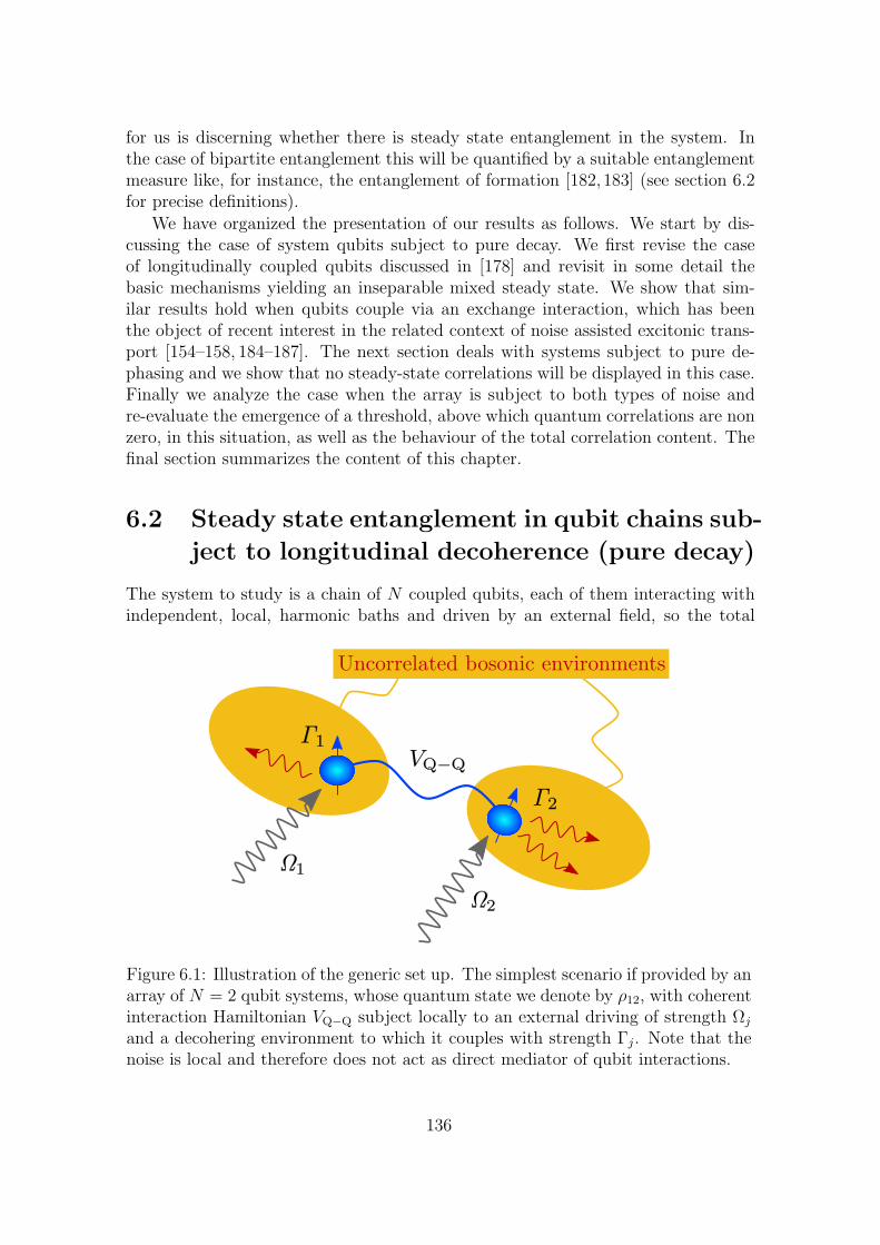
for us is discerning whether there is steady state entanglement in the system. Inthe case of bipartite entanglement this will be quantified by a suitable entanglementmeasure like, for instance, the entanglement of formation [182, 183] (see section 6.2for precise definitions).
We have organized the presentation of our results as follows. We start by dis-cussing the case of system qubits subject to pure decay. We first revise the caseof longitudinally coupled qubits discussed in [178] and revisit in some detail thebasic mechanisms yielding an inseparable mixed steady state. We show that sim-ilar results hold when qubits couple via an exchange interaction, which has beenthe object of recent interest in the related context of noise assisted excitonic trans-port [154–158, 184–187]. The next section deals with systems subject to pure de-phasing and we show that no steady-state correlations will be displayed in this case.Finally we analyze the case when the array is subject to both types of noise andre-evaluate the emergence of a threshold, above which quantum correlations are nonzero, in this situation, as well as the behaviour of the total correlation content. Thefinal section summarizes the content of this chapter.
6.2 Steady state entanglement in qubit chains sub-
ject to longitudinal decoherence (pure decay)
The system to study is a chain of N coupled qubits, each of them interacting withindependent, local, harmonic baths and driven by an external field, so the total
Figure 6.1: Illustration of the generic set up. The simplest scenario if provided by anarray of N = 2 qubit systems, whose quantum state we denote by ρ12, with coherentinteraction Hamiltonian VQ−Q subject locally to an external driving of strength Ωj
and a decohering environment to which it couples with strength Γj. Note that thenoise is local and therefore does not act as direct mediator of qubit interactions.
136
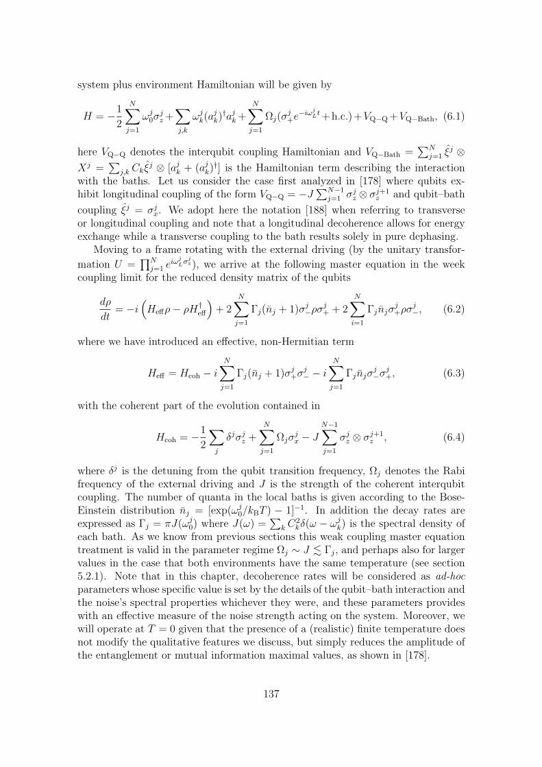
system plus environment Hamiltonian will be given by
H = −1
2
N∑j=1
ωj0σ
jz +
∑
j,k
ωjk(a
jk)†aj
k +N∑
j=1
Ωj(σj+e−iωj
Lt +h.c.)+VQ−Q +VQ−Bath, (6.1)
here VQ−Q denotes the interqubit coupling Hamiltonian and VQ−Bath =∑N
j=1 ξj ⊗Xj =
∑j,k Ckξ
j ⊗ [ajk + (aj
k)†] is the Hamiltonian term describing the interaction
with the baths. Let us consider the case first analyzed in [178] where qubits ex-hibit longitudinal coupling of the form VQ−Q = −J
∑N−1j=1 σj
z ⊗ σj+1z and qubit–bath
coupling ξj = σjx. We adopt here the notation [188] when referring to transverse
or longitudinal coupling and note that a longitudinal decoherence allows for energyexchange while a transverse coupling to the bath results solely in pure dephasing.
Moving to a frame rotating with the external driving (by the unitary transfor-
mation U =∏N
j=1 eiωjLσj
z), we arrive at the following master equation in the weekcoupling limit for the reduced density matrix of the qubits
dρ
dt= −i
(Heffρ− ρH†
eff
)+ 2
N∑j=1
Γj(nj + 1)σj−ρσj
+ + 2N∑
i=1
Γjnjσj+ρσj
−, (6.2)
where we have introduced an effective, non-Hermitian term
Heff = Hcoh − i
N∑j=1
Γj(nj + 1)σj+σj
− − i
N∑j=1
Γjnjσj−σj
+, (6.3)
with the coherent part of the evolution contained in
Hcoh = −1
2
∑j
δjσjz +
N∑j=1
Ωjσjx − J
N−1∑j=1
σjz ⊗ σj+1
z , (6.4)
where δj is the detuning from the qubit transition frequency, Ωj denotes the Rabifrequency of the external driving and J is the strength of the coherent interqubitcoupling. The number of quanta in the local baths is given according to the Bose-Einstein distribution nj = [exp(ωj
0/kBT ) − 1]−1. In addition the decay rates areexpressed as Γj = πJ(ωj
0) where J(ω) =∑
k C2kδ(ω − ωj
k) is the spectral density ofeach bath. As we know from previous sections this weak coupling master equationtreatment is valid in the parameter regime Ωj ∼ J . Γj, and perhaps also for largervalues in the case that both environments have the same temperature (see section5.2.1). Note that in this chapter, decoherence rates will be considered as ad-hocparameters whose specific value is set by the details of the qubit–bath interaction andthe noise’s spectral properties whichever they were, and these parameters provideswith an effective measure of the noise strength acting on the system. Moreover, wewill operate at T = 0 given that the presence of a (realistic) finite temperature doesnot modify the qualitative features we discuss, but simply reduces the amplitude ofthe entanglement or mutual information maximal values, as shown in [178].
137

Let us consider the simplest case where the arrays consist of only two qubitswhose state we will denote by ρ12, as depicted in figure 6.1, and let us assume, forsimplicity, that Ω1 = Ω2 = Ω and Γ1 = Γ2 = Γ. At perfect tuning δj = 0 and zerotemperature, the steady state of the master equation given by equation (6.2) can becomputed analytically to be [178]
ρss12 =
1
k
t2 + 4s2r2, 2sr2 + irt, 2sr2 + irt, 2irs− r2
2sr2 − irt, t, r2, ir2sr2 − irt, r2, t, ir−2irs− r2, −ir, −ir, 1
(6.5)
where k = 3 + 2r2 + t2 + 4r2s2, r = Γ/Ω, s = J/Ω and t = r2 + 1. This state isseparable if, and only if, its partial transpose is a positive operator [189]. We findthat ρss
12 is entangled for values of the noise strength Γ such that
Γ > Γth, where Γth =Ω2
2J. (6.6)
As a result, the systems exhibit quantum correlations in the steady state only if thenoise strength, encapsulated in the parameter Γ, is above the threshold value Γth.Otherwise, the steady state is fully separable. In order to shed light onto this rathercounterintuitive behaviour, it is useful to analyze the structural form of the steadystate density matrix by calculating its spectral resolution. One can easily evaluatethe eigenvalues of the density matrix specifying the steady state equation (6.5) tobe
λ1,2 =1
4r2s2 + (1 + t)2,
λ3,4 =1 + r2 (2 + 4s2) + t2 ∓
√4r2 (1 + s2) + (t− 1)2
√4r2s2 + (1 + t)2
2 (4r2s2 + (1 + t)2).
The corresponding expressions for the eigenvectors are not so compact. Figure 6.2shows these eigenvalues as a function of the noise strength as well as the steadystate entanglement as measured by the entanglement of formation EF (ρ12). Thisquantity represents the minimal possible average entanglement over all pure statedecomposition of ρ and as such, its evaluation requires solving a variational problem.However, in the case of two qubits, the entanglement of formation has a simpleclosed form in terms of the so-called two-qubit concurrence, defined as C(ρ) =max0, µ1 − µ2 − µ3 − µ4, where the µi are, in decreasing order, the eigenvalues ofthe matrix ρσy ⊗ σyρ
∗σy ⊗ σy, where ρ∗ is the matrix obtained by element complexconjugation of ρ [182]. For any bipartite qubit state,
EF (ρ) = s
(1 +
√1− C2(ρ)
2
), (6.7)
where s(x) = −x log2 x − (1 − x) log2(1 − x). We see in figure 6.2 that the entan-glement of formation is zero for noise values below threshold, while displaying the
138
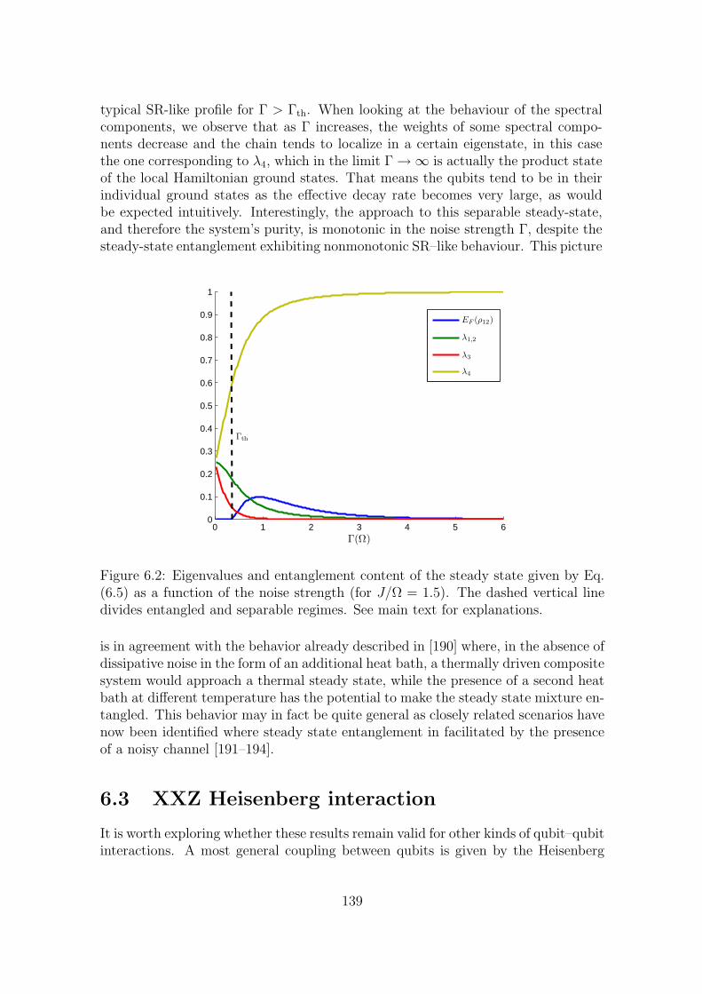
typical SR-like profile for Γ > Γth. When looking at the behaviour of the spectralcomponents, we observe that as Γ increases, the weights of some spectral compo-nents decrease and the chain tends to localize in a certain eigenstate, in this casethe one corresponding to λ4, which in the limit Γ →∞ is actually the product stateof the local Hamiltonian ground states. That means the qubits tend to be in theirindividual ground states as the effective decay rate becomes very large, as wouldbe expected intuitively. Interestingly, the approach to this separable steady-state,and therefore the system’s purity, is monotonic in the noise strength Γ, despite thesteady-state entanglement exhibiting nonmonotonic SR–like behaviour. This picture
0 1 2 3 4 5 60
0.1
0.2
0.3
0.4
0.5
0.6
0.7
0.8
0.9
1
Γ(Ω)
EF (ρ12)
λ1,2
λ3
λ4
Γth
Figure 6.2: Eigenvalues and entanglement content of the steady state given by Eq.(6.5) as a function of the noise strength (for J/Ω = 1.5). The dashed vertical linedivides entangled and separable regimes. See main text for explanations.
is in agreement with the behavior already described in [190] where, in the absence ofdissipative noise in the form of an additional heat bath, a thermally driven compositesystem would approach a thermal steady state, while the presence of a second heatbath at different temperature has the potential to make the steady state mixture en-tangled. This behavior may in fact be quite general as closely related scenarios havenow been identified where steady state entanglement in facilitated by the presenceof a noisy channel [191–194].
6.3 XXZ Heisenberg interaction
It is worth exploring whether these results remain valid for other kinds of qubit–qubitinteractions. A most general coupling between qubits is given by the Heisenberg
139
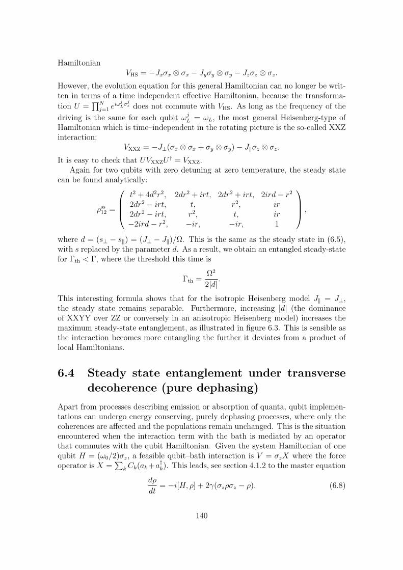
HamiltonianVHS = −Jxσx ⊗ σx − Jyσy ⊗ σy − Jzσz ⊗ σz.
However, the evolution equation for this general Hamiltonian can no longer be writ-ten in terms of a time independent effective Hamiltonian, because the transforma-
tion U =∏N
j=1 eiωjLσj
z does not commute with VHS. As long as the frequency of the
driving is the same for each qubit ωjL = ωL, the most general Heisenberg-type of
Hamiltonian which is time–independent in the rotating picture is the so-called XXZinteraction:
VXXZ = −J⊥(σx ⊗ σx + σy ⊗ σy)− J‖σz ⊗ σz.
It is easy to check that UVXXZU† = VXXZ.
Again for two qubits with zero detuning at zero temperature, the steady statecan be found analytically:
ρss12 =
t2 + 4d2r2, 2dr2 + irt, 2dr2 + irt, 2ird− r2
2dr2 − irt, t, r2, ir2dr2 − irt, r2, t, ir−2ird− r2, −ir, −ir, 1
,
where d = (s⊥ − s‖) = (J⊥ − J‖)/Ω. This is the same as the steady state in (6.5),with s replaced by the parameter d. As a result, we obtain an entangled steady-statefor Γth < Γ, where the threshold this time is
Γth =Ω2
2|d| .
This interesting formula shows that for the isotropic Heisenberg model J‖ = J⊥,the steady state remains separable. Furthermore, increasing |d| (the dominanceof XXYY over ZZ or conversely in an anisotropic Heisenberg model) increases themaximum steady-state entanglement, as illustrated in figure 6.3. This is sensible asthe interaction becomes more entangling the further it deviates from a product oflocal Hamiltonians.
6.4 Steady state entanglement under transverse
decoherence (pure dephasing)
Apart from processes describing emission or absorption of quanta, qubit implemen-tations can undergo energy conserving, purely dephasing processes, where only thecoherences are affected and the populations remain unchanged. This is the situationencountered when the interaction term with the bath is mediated by an operatorthat commutes with the qubit Hamiltonian. Given the system Hamiltonian of onequbit H = (ω0/2)σz, a feasible qubit–bath interaction is V = σzX where the forceoperator is X =
∑k Ck(ak +a†k). This leads, see section 4.1.2 to the master equation
dρ
dt= −i[H, ρ] + 2γ(σzρσz − ρ). (6.8)
140

0 0.2 0.4 0.6 0.8 1 1.2 1.4 1.6 1.8 20
0.02
0.04
0.06
0.08
0.1
0.12
0.14
0.16
Γ(Ω)
EF(ρ
12)
|d| = 4|d| = 3|d| = 2|d| = 1|d| = 0
Figure 6.3: Increasing behaviour of the steady-state entanglement for |d| growingfrom 0 to 4. The system is separable when d = 0 (isotropic Heisenberg model).When d increases, and the term XXYY dominates, the range of values of Γ forwhich the steady state is separable shrinks, while the maximum achievable steadystate entanglement grows.
This process can be embedded in our framework provided that the Rabi frequen-cies of the external driving Ωj and the interqubit coupling J are small enough. Themaster equation in the rotating picture for N qubits is then given by
dρ
dt= −i[Hcoh, ρ] + 2
N∑j=1
γj(σjzρσj
z − ρ). (6.9)
In this situation the system no longer exhibits quantum correlations in the steadystate. Indeed, the steady state of equation (6.9) is unique and it is the completelymixed state ρss = 1/N . This result follows from theorem 5.2 in [67] which assertsthat given a steady state ρss of a master equation written in the standard form
dρ
dt= −i[H, ρ] +
∑j
(VjρV †
j −1
2V †
j Vjρ− 1
2ρV †
j Vj
),
such that rank(ρss) = N , the given steady state is unique if the only operatorscommuting with H and every Vj are multiples of the identity. This is true for ourcase since the only operators that commute with both σx and σz (and therefore withσy as well because of the Jacobi identity) are proportional to the identity becauseof Schur’s lemma.
141
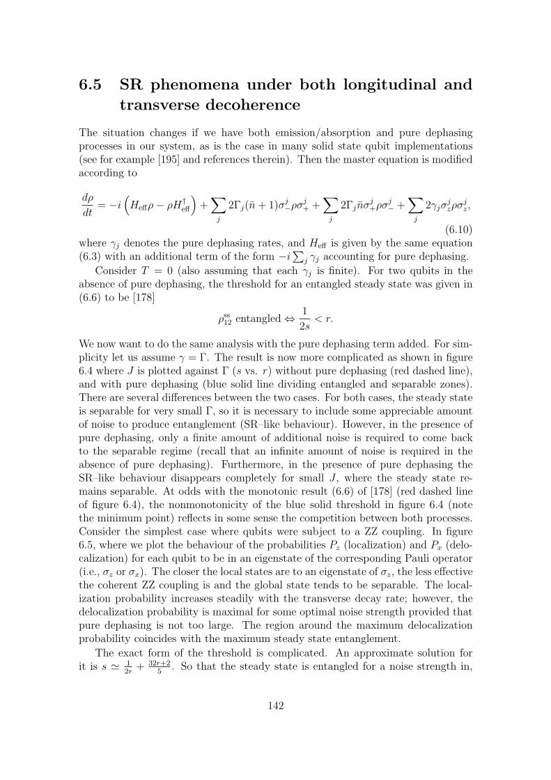
6.5 SR phenomena under both longitudinal and
transverse decoherence
The situation changes if we have both emission/absorption and pure dephasingprocesses in our system, as is the case in many solid state qubit implementations(see for example [195] and references therein). Then the master equation is modifiedaccording to
dρ
dt= −i
(Heffρ− ρH†
eff
)+
∑j
2Γj(n + 1)σj−ρσj
+ +∑
j
2Γjnσj+ρσj
− +∑
j
2γjσjzρσj
z,
(6.10)where γj denotes the pure dephasing rates, and Heff is given by the same equation(6.3) with an additional term of the form −i
∑j γj accounting for pure dephasing.
Consider T = 0 (also assuming that each γj is finite). For two qubits in theabsence of pure dephasing, the threshold for an entangled steady state was given in(6.6) to be [178]
ρss12 entangled ⇔ 1
2s< r.
We now want to do the same analysis with the pure dephasing term added. For sim-plicity let us assume γ = Γ. The result is now more complicated as shown in figure6.4 where J is plotted against Γ (s vs. r) without pure dephasing (red dashed line),and with pure dephasing (blue solid line dividing entangled and separable zones).There are several differences between the two cases. For both cases, the steady stateis separable for very small Γ, so it is necessary to include some appreciable amountof noise to produce entanglement (SR–like behaviour). However, in the presence ofpure dephasing, only a finite amount of additional noise is required to come backto the separable regime (recall that an infinite amount of noise is required in theabsence of pure dephasing). Furthermore, in the presence of pure dephasing theSR–like behaviour disappears completely for small J , where the steady state re-mains separable. At odds with the monotonic result (6.6) of [178] (red dashed lineof figure 6.4), the nonmonotonicity of the blue solid threshold in figure 6.4 (notethe minimum point) reflects in some sense the competition between both processes.Consider the simplest case where qubits were subject to a ZZ coupling. In figure6.5, where we plot the behaviour of the probabilities Pz (localization) and Px (delo-calization) for each qubit to be in an eigenstate of the corresponding Pauli operator(i.e., σz or σx). The closer the local states are to an eigenstate of σz, the less effectivethe coherent ZZ coupling is and the global state tends to be separable. The local-ization probability increases steadily with the transverse decay rate; however, thedelocalization probability is maximal for some optimal noise strength provided thatpure dephasing is not too large. The region around the maximum delocalizationprobability coincides with the maximum steady state entanglement.
The exact form of the threshold is complicated. An approximate solution forit is s ' 1
2r+ 32r+2
5. So that the steady state is entangled for a noise strength in,
142
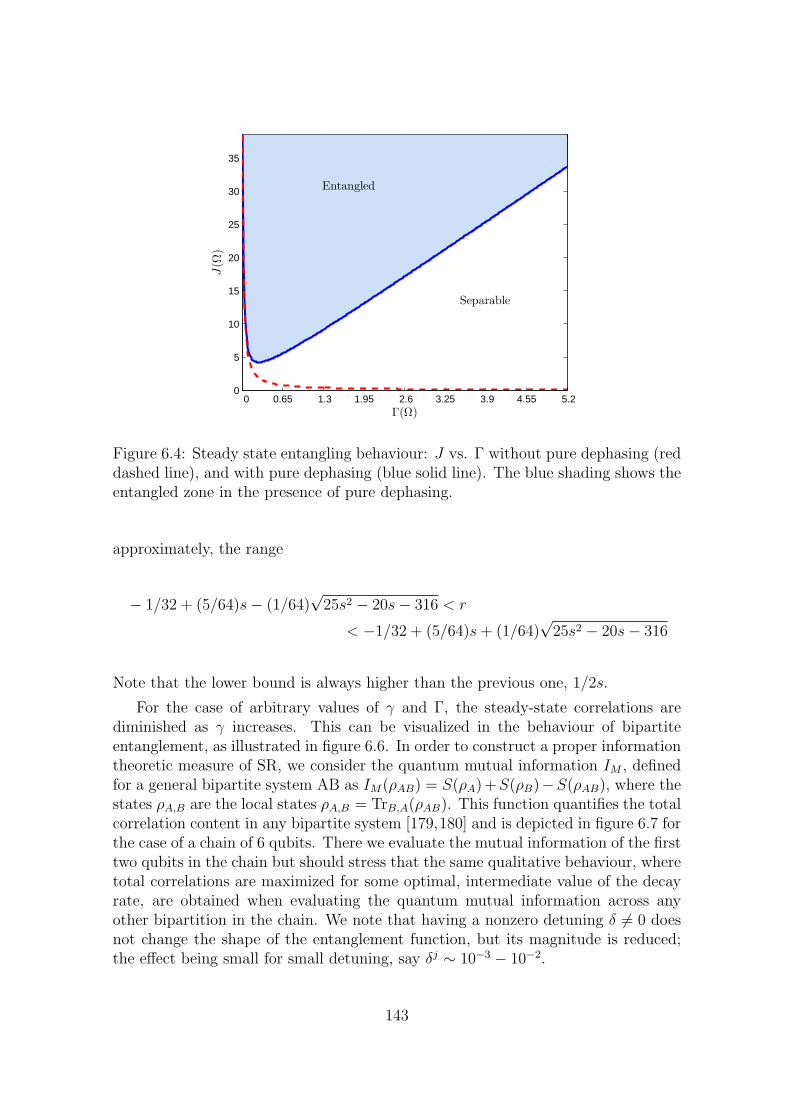
0 0.65 1.3 1.95 2.6 3.25 3.9 4.55 5.20
5
10
15
20
25
30
35
Γ(Ω)
J(Ω
)
Entangled
Separable
Figure 6.4: Steady state entangling behaviour: J vs. Γ without pure dephasing (reddashed line), and with pure dephasing (blue solid line). The blue shading shows theentangled zone in the presence of pure dephasing.
approximately, the range
− 1/32 + (5/64)s− (1/64)√
25s2 − 20s− 316 < r
< −1/32 + (5/64)s + (1/64)√
25s2 − 20s− 316
Note that the lower bound is always higher than the previous one, 1/2s.
For the case of arbitrary values of γ and Γ, the steady-state correlations arediminished as γ increases. This can be visualized in the behaviour of bipartiteentanglement, as illustrated in figure 6.6. In order to construct a proper informationtheoretic measure of SR, we consider the quantum mutual information IM , definedfor a general bipartite system AB as IM(ρAB) = S(ρA)+S(ρB)−S(ρAB), where thestates ρA,B are the local states ρA,B = TrB,A(ρAB). This function quantifies the totalcorrelation content in any bipartite system [179,180] and is depicted in figure 6.7 forthe case of a chain of 6 qubits. There we evaluate the mutual information of the firsttwo qubits in the chain but should stress that the same qualitative behaviour, wheretotal correlations are maximized for some optimal, intermediate value of the decayrate, are obtained when evaluating the quantum mutual information across anyother bipartition in the chain. We note that having a nonzero detuning δ 6= 0 doesnot change the shape of the entanglement function, but its magnitude is reduced;the effect being small for small detuning, say δj ∼ 10−3 − 10−2.
143
0 1 2 3 4 50.5
0.6
0.7
0.8
0.9
1
Γ(Ω)
Pz(ρ1)
Px(ρ1)
γ(Ω) = 0γ(Ω) = 2/3γ(Ω) = 4/3γ(Ω) = 2
Figure 6.5: Illustration of the combined action of transverse and longitudinal deco-herence on an array of N = 2 qubits with a ZZ interqubit Hamiltonian. Increasingthe pure dephasing rate keeps the delocalization probability of single qubits Px closeto 1/2 so that the qubits are in a state close to an eigenstate of their local Hamil-tonians (σz) which reduces the entangling power of the coherent ZZ coupling.
6.6 Conclusion
In this chapter we have discussed the emergence of SR–like effects in compositespin systems subject to both decay (longitudinal decoherence) and pure dephasing(transverse decoherence). We have shown that quantum correlations vanish in thesteady state if the local noise is purely transverse. Under pure dephasing, thesystem evolves into a maximally mixed state. When transverse and longitudinalnoise are simultaneously present, for fixed dephasing, one encounters a decay ratethreshold for steady–state entanglement to exist, provided that dephasing noiseremains moderate. In the special case where Γ = γ, an approximate analyticalthreshold condition can be derived.
To quantitatively characterize the presence of stochastic resonance, we computethe total correlation content of the system, as quantified by its mutual informationfor bipartitions of arbitrary size, and show that it is a non-monotonic function ofthe decay rate Γ (for fixed γ). We therefore argue that the system displays SR asmeasured by an information–theoretic figure of merit.
In this regard we have focussed our interest on the correlations content and, inparticular, on the entanglement content of the steady state. These results show thata noisy environment does not just monotonically degrade the amount of entangle-
144
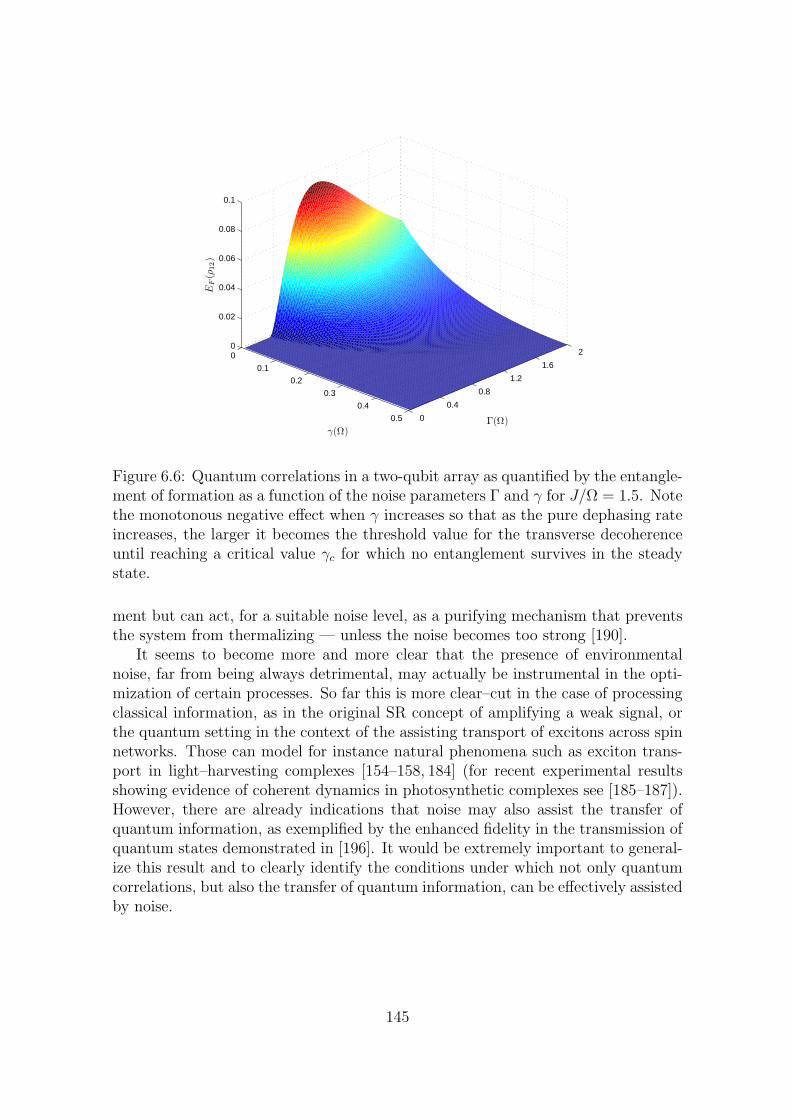
0
0.1
0.2
0.3
0.4
0.5 0
0.4
0.8
1.2
1.6
20
0.02
0.04
0.06
0.08
0.1
Γ(Ω)γ(Ω)
EF(ρ
12)
Figure 6.6: Quantum correlations in a two-qubit array as quantified by the entangle-ment of formation as a function of the noise parameters Γ and γ for J/Ω = 1.5. Notethe monotonous negative effect when γ increases so that as the pure dephasing rateincreases, the larger it becomes the threshold value for the transverse decoherenceuntil reaching a critical value γc for which no entanglement survives in the steadystate.
ment but can act, for a suitable noise level, as a purifying mechanism that preventsthe system from thermalizing — unless the noise becomes too strong [190].
It seems to become more and more clear that the presence of environmentalnoise, far from being always detrimental, may actually be instrumental in the opti-mization of certain processes. So far this is more clear–cut in the case of processingclassical information, as in the original SR concept of amplifying a weak signal, orthe quantum setting in the context of the assisting transport of excitons across spinnetworks. Those can model for instance natural phenomena such as exciton trans-port in light–harvesting complexes [154–158, 184] (for recent experimental resultsshowing evidence of coherent dynamics in photosynthetic complexes see [185–187]).However, there are already indications that noise may also assist the transfer ofquantum information, as exemplified by the enhanced fidelity in the transmission ofquantum states demonstrated in [196]. It would be extremely important to general-ize this result and to clearly identify the conditions under which not only quantumcorrelations, but also the transfer of quantum information, can be effectively assistedby noise.
145
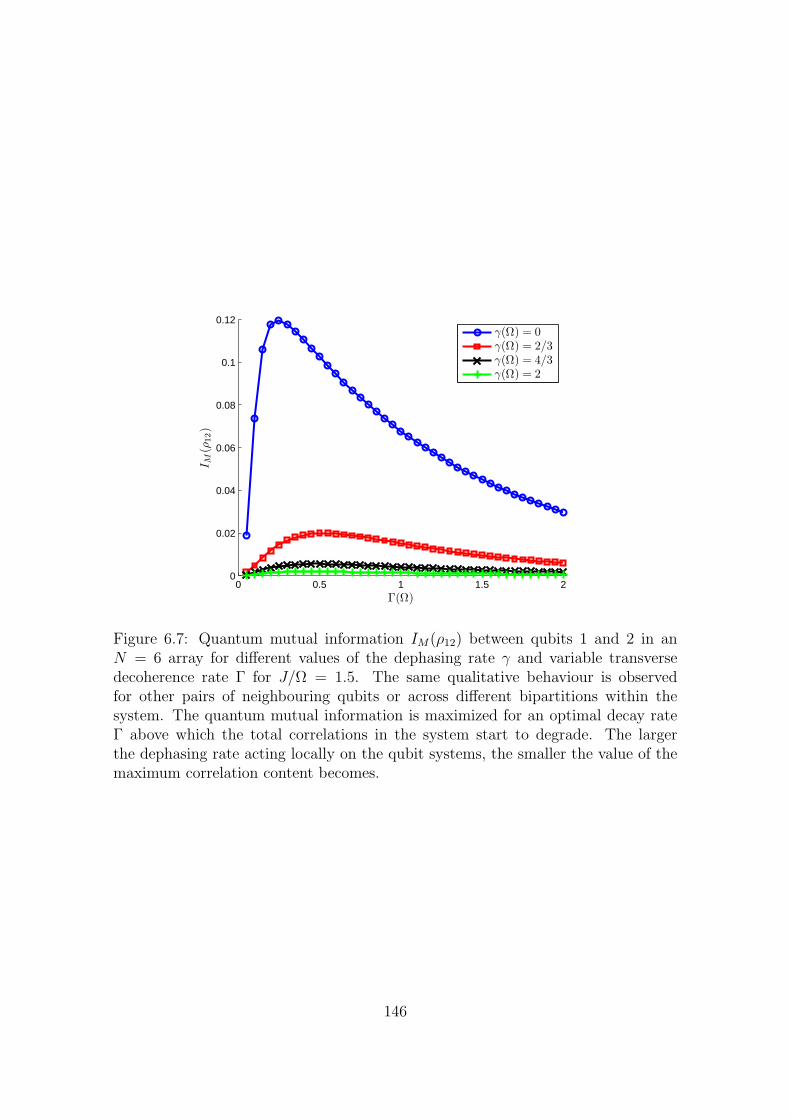
0 0.5 1 1.5 20
0.02
0.04
0.06
0.08
0.1
0.12
Γ(Ω)
I M(ρ
12)
γ(Ω) = 0γ(Ω) = 2/3γ(Ω) = 4/3γ(Ω) = 2
Figure 6.7: Quantum mutual information IM(ρ12) between qubits 1 and 2 in anN = 6 array for different values of the dephasing rate γ and variable transversedecoherence rate Γ for J/Ω = 1.5. The same qualitative behaviour is observedfor other pairs of neighbouring qubits or across different bipartitions within thesystem. The quantum mutual information is maximized for an optimal decay rateΓ above which the total correlations in the system start to degrade. The largerthe dephasing rate acting locally on the qubit systems, the smaller the value of themaximum correlation content becomes.
146
Part III
Identifying Elements ofnon-Markovianity
147

Chapter 7
Measures of non-Markovianity
7.1 Introduction
As we know, the actual dynamics of any real open quantum system is expectedto deviate to some extent from the idealized Markovian evolution that arises fromthe conditions of weak (or singular) coupling to a memoryless reservoir. Whilequantum optics provides realizations that are extremely well approximated by suchan evolution, soft or condensed matter systems evolve subject to conditions that aregenerally unsuited to be treated within the Markovian framework. The exact detailsof what makes a given quantum evolution non-Markovian may be complicated, andin many cases, especially when thinking about many-body systems, an accuratemicroscopic model of the system-bath interaction may actually be unfeasible. Itwould therefore be very useful to define some simple measure that captures, in someform, the fact that the evolution departs from strict Markovianity.
Here, we propose two possible ways to quantify the non-Markovian character ofa quantum evolution which avoid the definition of an optimization problem. Ourkey element will be exploiting the specific behavior of quantum correlations whena part of a composite system is subject to a local interaction that can be modeledas a trace-preserving CP map. This will allow us to give a necessary condition tomeasure deviations from Markovianity even when the actual form of the dynamics iscompletely unknown, although some non-Markovian evolutions may be undetected.A necessary and sufficient condition can be provided in the case when the dynamicsis amenable to complete characterization, for instance, via quantum process tomog-raphy. In this case, we are able to quantify strictly the Markovian character of theevolution and deviations from strict Markovianity can be unambiguously character-ized.
7.2 Previous attempts
Before explaining our proposal, for the sake of completeness we revise some otherapproaches for the assessment of non-Markovianity in this section.
149
7.2.1 Proposal of Wolf et. al.
The problem of quantifying non-Markovinity was addressed by Wolf and collabora-tors in the context of abstract quantum channels [197]. In their case, a “snapshot”of the dynamics at some time t1 is given, E ≡ E(t1,t0), and they ask whether sucha quantum channel E can be written as part of a completely positive semigroup,this is, E = eL, where L is of the form of (3.33). For that purpose, they take thelogarithm of E , and look if any of its branches is of the form of (3.33). If the answeris negative, they quantify the amount of non-Markoviniaty as the minimum amountµ of isotropic noise Eiso(ρ) = e−µρ + (1 − e−µ)1/d, such that log(E) + log(Eiso) isa generator of the form (3.33). Unfortunately the extension of this approach totime-dependent Markovian process is not available.
7.2.2 Proposal of Breuer et. al.
Very recently, Breuer and collaborators proposed an optimization-based measure ofnon-Markovianity founded upon the behavior of the trace distance under completelypositive and trace-preserving maps (CPT) [198]. They consider the evolution of thetrace distance of two quantum states ‖ρ1(t) − ρ2(t)‖ under some evolution. As weproved in section 3.2.3, UDMs are contractions for the trace norm, and in particularthey are contractions for the trace distance. Since Markovian evolutions are divisiblein UDMs (see definition 3.2.6) the trace distance has to be monotonically decreasingwith the time. Breuer et. al. suggested considering as a degree of non-Markovianitythe maximum increment of the trace distance for arbitrary pairs of initial statesρ1,2(0). Leaving aside minor considerations, the main problem of this approach isthe hard optimization which is required.
7.2.3 Geometric measures
Conceptually, one could think of introducing a Markovianity measure via some typeof geometric optimization problem, such as evaluating a quantity of the form
maxε>0
minEM
‖E(t0+ε,t0) − EM(t0+ε,t0)‖,
where ‖ · ‖ denotes some appropriate operator norm. The minimum is taken overthe set of Markovian maps EM , while the maximum over final times accounts forthe time-continuous dependence of the dynamical maps (note that E(t0,t0) = 1 in-dependently of E , and 1 is trivially Markovian). However, this quantity is hard tocompute in practice due to the nonconvex structure of the set of Markovian mapsEM [197].
7.2.4 Microscopic approach
If the starting point is some microscopic model, a different approach would be toexploit the fact that the dynamics will tend to be Markovian when it is possible
150
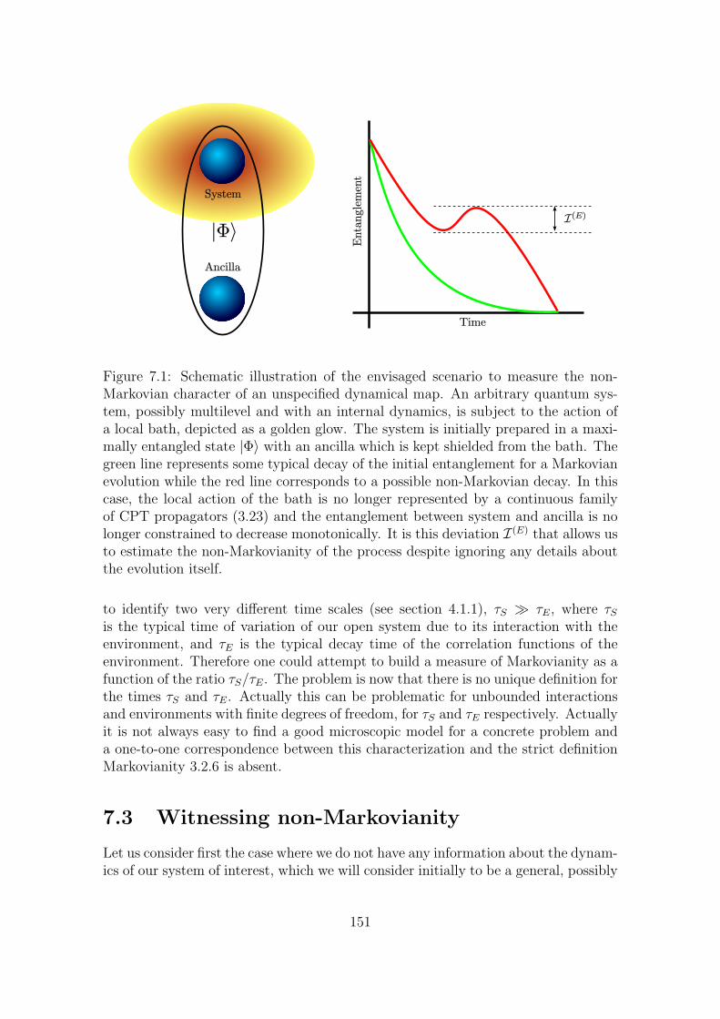
Figure 7.1: Schematic illustration of the envisaged scenario to measure the non-Markovian character of an unspecified dynamical map. An arbitrary quantum sys-tem, possibly multilevel and with an internal dynamics, is subject to the action ofa local bath, depicted as a golden glow. The system is initially prepared in a maxi-mally entangled state |Φ〉 with an ancilla which is kept shielded from the bath. Thegreen line represents some typical decay of the initial entanglement for a Markovianevolution while the red line corresponds to a possible non-Markovian decay. In thiscase, the local action of the bath is no longer represented by a continuous familyof CPT propagators (3.23) and the entanglement between system and ancilla is nolonger constrained to decrease monotonically. It is this deviation I(E) that allows usto estimate the non-Markovianity of the process despite ignoring any details aboutthe evolution itself.
to identify two very different time scales (see section 4.1.1), τS À τE, where τS
is the typical time of variation of our open system due to its interaction with theenvironment, and τE is the typical decay time of the correlation functions of theenvironment. Therefore one could attempt to build a measure of Markovianity as afunction of the ratio τS/τE. The problem is now that there is no unique definition forthe times τS and τE. Actually this can be problematic for unbounded interactionsand environments with finite degrees of freedom, for τS and τE respectively. Actuallyit is not always easy to find a good microscopic model for a concrete problem anda one-to-one correspondence between this characterization and the strict definitionMarkovianity 3.2.6 is absent.
7.3 Witnessing non-Markovianity
Let us consider first the case where we do not have any information about the dynam-ics of our system of interest, which we will consider initially to be a general, possibly
151
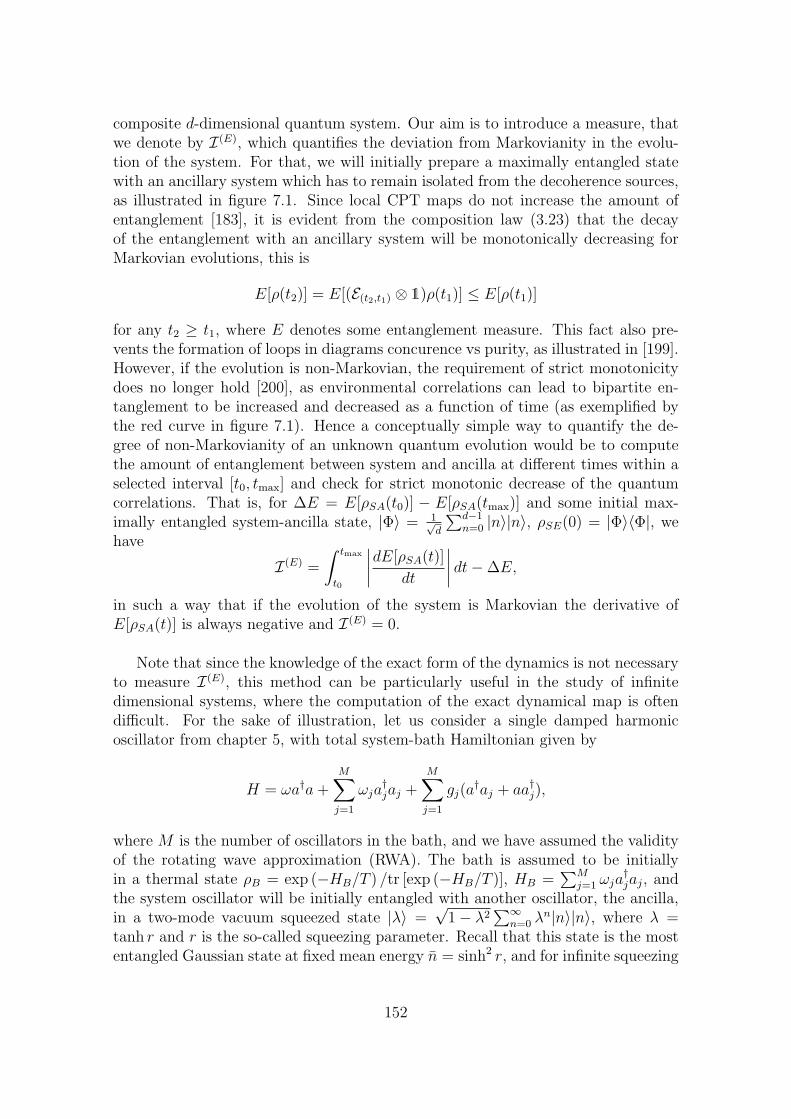
composite d-dimensional quantum system. Our aim is to introduce a measure, thatwe denote by I(E), which quantifies the deviation from Markovianity in the evolu-tion of the system. For that, we will initially prepare a maximally entangled statewith an ancillary system which has to remain isolated from the decoherence sources,as illustrated in figure 7.1. Since local CPT maps do not increase the amount ofentanglement [183], it is evident from the composition law (3.23) that the decayof the entanglement with an ancillary system will be monotonically decreasing forMarkovian evolutions, this is
E[ρ(t2)] = E[(E(t2,t1) ⊗ 1)ρ(t1)] ≤ E[ρ(t1)]
for any t2 ≥ t1, where E denotes some entanglement measure. This fact also pre-vents the formation of loops in diagrams concurence vs purity, as illustrated in [199].However, if the evolution is non-Markovian, the requirement of strict monotonicitydoes no longer hold [200], as environmental correlations can lead to bipartite en-tanglement to be increased and decreased as a function of time (as exemplified bythe red curve in figure 7.1). Hence a conceptually simple way to quantify the de-gree of non-Markovianity of an unknown quantum evolution would be to computethe amount of entanglement between system and ancilla at different times within aselected interval [t0, tmax] and check for strict monotonic decrease of the quantumcorrelations. That is, for ∆E = E[ρSA(t0)] − E[ρSA(tmax)] and some initial max-imally entangled system-ancilla state, |Φ〉 = 1√
d
∑d−1n=0 |n〉|n〉, ρSE(0) = |Φ〉〈Φ|, we
have
I(E) =
∫ tmax
t0
∣∣∣∣dE[ρSA(t)]
dt
∣∣∣∣ dt−∆E,
in such a way that if the evolution of the system is Markovian the derivative ofE[ρSA(t)] is always negative and I(E) = 0.
Note that since the knowledge of the exact form of the dynamics is not necessaryto measure I(E), this method can be particularly useful in the study of infinitedimensional systems, where the computation of the exact dynamical map is oftendifficult. For the sake of illustration, let us consider a single damped harmonicoscillator from chapter 5, with total system-bath Hamiltonian given by
H = ωa†a +M∑
j=1
ωja†jaj +
M∑j=1
gj(a†aj + aa†j),
where M is the number of oscillators in the bath, and we have assumed the validityof the rotating wave approximation (RWA). The bath is assumed to be initiallyin a thermal state ρB = exp (−HB/T ) /tr [exp (−HB/T )], HB =
∑Mj=1 ωja
†jaj, and
the system oscillator will be initially entangled with another oscillator, the ancilla,in a two-mode vacuum squeezed state |λ〉 =
√1− λ2
∑∞n=0 λn|n〉|n〉, where λ =
tanh r and r is the so-called squeezing parameter. Recall that this state is the mostentangled Gaussian state at fixed mean energy n = sinh2 r, and for infinite squeezing
152
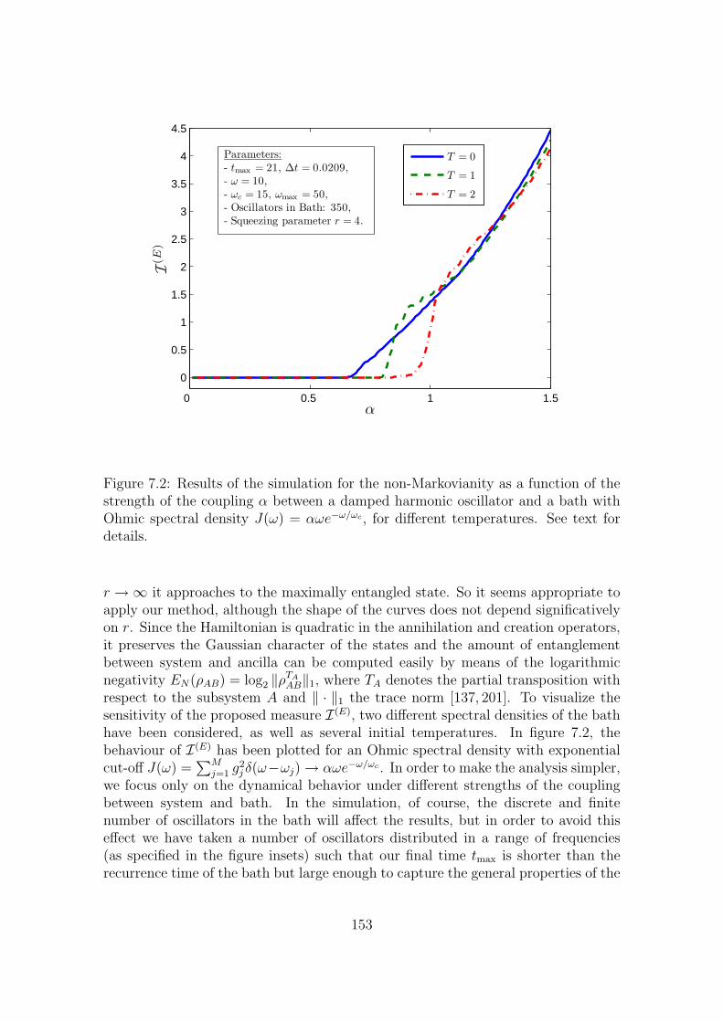
0 0.5 1 1.5
0
0.5
1
1.5
2
2.5
3
3.5
4
4.5
α
I(E
)
T = 0
T = 1
T = 2
Parameters:
- tmax = 21, ∆t = 0.0209,
- ω = 10,
- ωc = 15, ωmax = 50,
- Oscillators in Bath: 350,
- Squeezing parameter r = 4.
Figure 7.2: Results of the simulation for the non-Markovianity as a function of thestrength of the coupling α between a damped harmonic oscillator and a bath withOhmic spectral density J(ω) = αωe−ω/ωc , for different temperatures. See text fordetails.
r →∞ it approaches to the maximally entangled state. So it seems appropriate toapply our method, although the shape of the curves does not depend significativelyon r. Since the Hamiltonian is quadratic in the annihilation and creation operators,it preserves the Gaussian character of the states and the amount of entanglementbetween system and ancilla can be computed easily by means of the logarithmicnegativity EN(ρAB) = log2 ‖ρTA
AB‖1, where TA denotes the partial transposition withrespect to the subsystem A and ‖ · ‖1 the trace norm [137, 201]. To visualize thesensitivity of the proposed measure I(E), two different spectral densities of the bathhave been considered, as well as several initial temperatures. In figure 7.2, thebehaviour of I(E) has been plotted for an Ohmic spectral density with exponentialcut-off J(ω) =
∑Mj=1 g2
j δ(ω−ωj) → αωe−ω/ωc . In order to make the analysis simpler,we focus only on the dynamical behavior under different strengths of the couplingbetween system and bath. In the simulation, of course, the discrete and finitenumber of oscillators in the bath will affect the results, but in order to avoid thiseffect we have taken a number of oscillators distributed in a range of frequencies(as specified in the figure insets) such that our final time tmax is shorter than therecurrence time of the bath but large enough to capture the general properties of the
153
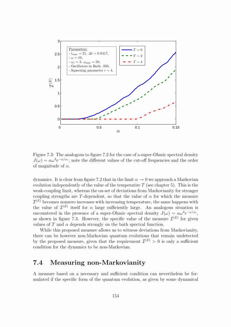
0 0.5 0.1 0.15
0
0.5
1
1.5
2
2.5
3
α
I(E
)
T = 0
T = 2
T = 4
Parameters:
- tmax = 21, ∆t = 0.0417,
- ω = 10,
- ωc = 3, ωmax = 50,
- Oscillators in Bath: 350,
- Squeezing parameter r = 4.
Figure 7.3: The analogous to figure 7.2 for the case of a super-Ohmic spectral densityJ(ω) = αω3e−ω/ωc ; note the different values of the cut-off frequencies and the orderof magnitude of α.
dynamics. It is clear from figure 7.2 that in the limit α → 0 we approach a Markovianevolution independently of the value of the temperatire T (see chapter 5). This is theweak-coupling limit, whereas the on-set of deviations from Markovianity for strongercoupling strengths are T -dependent, so that the value of α for which the measureI(E) becomes nonzero increases with increasing temperature, the same happens withthe value of I(E) itself for α large sufficiently large. An analogous situation isencountered in the presence of a super-Ohmic spectral density J(ω) = αω3e−ω/ωc ,as shown in figure 7.3. However, the specific value of the measure I(E) for givenvalues of T and α depends strongly on the bath spectral function.
While this proposed measure allows us to witness deviations from Markovianity,there can be however non-Markovian quantum evolutions that remain undetectedby the proposed measure, given that the requirement I(E) > 0 is only a sufficientcondition for the dynamics to be non-Markovian.
7.4 Measuring non-Markovianity
A measure based on a necessary and sufficient condition can nevertheless be for-mulated if the specific form of the quantum evolution, as given by some dynamical
154
map E(t,t0), is amenable to exact reconstruction between the some initial time t0 anda final time t. This can in principle be done by means of process tomography orperhaps resorting to a theoretical microscopic model. In order to construct such ameasure avoiding optimization problems, we will resort to the Choi-JamioÃlkowskicriterion [202] about completely positive maps which asserts the following:
7.4.1. Theorem (Choi-JamioÃlkowski criterion). A linear map E on the op-erators acting on a Hilbert space H (of finite dimension d) is completely positive ifand only if
(E ⊗ 1) |Φ〉〈Φ| ≥ 0, (7.1)
where |Φ〉 is the maximally entangled state in the space H⊗H.
Proof. By definition if E is completely positive then (7.1) is fulfilled as |Φ〉〈Φ| isa positive semidefinite matrix.
Conversely, assume that a map E satisfies the condition (7.1). Then consider anarbitrary state |ψ〉 =
∑i ci|i〉 and its complex conjugate |ψ∗〉 =
∑i c∗i |i〉, and notice
that
d〈ψ∗| [(E ⊗ 1) |Φ〉〈Φ|] |ψ∗〉 = d〈ψ∗|[
1
d
∑i,j
E (|i〉〈j|)⊗ |i〉〈j|]|ψ∗〉
=∑i,j
E (|i〉〈j|) 〈ψ∗|i〉〈j|ψ∗〉
=∑i,j
cic∗jE (|i〉〈j|) = E (|ψ〉〈ψ|) . (7.2)
In addition, using the spectral decomposition
d (E ⊗ 1) |Φ〉〈Φ| =∑
i
λi|si〉〈si|,
with λi ≥ 0 by presupposition, allows us to define the linear maps
Ki|ψ〉 =√
λi〈ψ∗|si〉,
for every state |ψ〉, and we have
∑i
Ki|ψ〉〈ψ|K†i =
∑i
λi〈ψ∗|si〉〈si|ψ∗〉 = d〈ψ∗| [(E ⊗ 1) |Φ〉〈Φ|] |ψ∗〉.
Thus by equation (7.2), E (|ψ〉〈ψ|) =∑
i Ki|ψ〉〈ψ|K†i . Finally by linearity the result
follows for any state ρ =∑
i pi|ψi〉〈ψi|,
E (ρ) =∑
i
KiρK†i ,
155
which is the Kraus decomposition of E and therefore completely positive (see section3.2.2). 2
Now, let us come back to the problem of constructing a measure of non-Markov-ianity, for definiteness take our initial time as t0 = 0 without loss of generality.Then, because of the continuity of time, we can split the known dynamical mapE(t,0) as
E(t+ε,0) = E(t+ε,t)E(t,0) (7.3)
for any times t and ε. If the time evolution implemented by E(t,0) is Markovian,E(t2,t1) is CPT for any intermediate times (t + ε) ≥ t2 ≥ t1 ≥ 0 (that is equivalent toE(t,0) be infinitesimally divisible in the sense of [197] for any t). However if and onlyif there exist times t and ε such that E(t+ε,t) is not completely positive, the dynamicswill be non-Markovian. Note that this is the ultimate reason behind the possibleincrease of the system-ancilla entanglement at some local times, which is the basisof our previous measure. This partition can be extracted from the known dynamicalmap E(t,0) as a function of t just by applying E−1
(t,0) (which may not be a completely
positive map) to the Eq. (7.3),
E(t+ε,t) = E(t+ε,0)E−1(t,0).
Since E(t→0,0) → 1, for t small enough, E(t,0) will be invertible. If for larger timesE(t,0) is not invertible, this means that we do not have enough information to defineE(t+ε,t) in an unequivocal way. This is one consequence of being blind to one partof the whole system, typically, the non-Markovianity will turn out to be infinity inthat case.
Next, the Choi-JamioÃlkowski criterion ensures that E(t+ε,t) is completely positiveif and only if
(E(t+ε,t) ⊗ 1) |Φ〉〈Φ| ≥ 0. Hence, given the trace-preserving property,
we can take the following definition as a measure of the non-CP character of E(t+ε,t),
fNCP (t + ε, t) = ‖ (E(t+ε,t) ⊗ 1)(|Φ〉〈Φ|) ‖1.
Thus, E(t+ε,t) is CPT if and only if fNCP (t + ε, t) = 1, otherwise fNCP (t + ε, t) > 1.Now fNCP (t + ε, t) will be the building block of our measure of non-Markovianity.To construct it we leave ε to be infinitesimal to define the (right) derivative offNCP (t + ε, t):
g(t) = limε→0+
fNCP (t + ε, t)− 1
ε,
noticing that g(t) ≥ 0, with g(t) = 0 if and only if E(t+ε,t) is CPT. Therefore theintegral
I =
∫ tf
0
g(t)dt
can be taken as a measure of non-Markovianity between 0 and some final time tf(in fact, if we know completely the dynamics, we can take tf → ∞). Actually a
normalized version of this measure may be D(ratio)NM = I
I+1or D(exp)
NM = 1 − e−I , in
156
such a way that DNM = 0 for I = 0 (i.e. Markovian evolution) and DNM → 1 forI → ∞.
To illustrate the behaviour of I, let us consider the dynamics of one qubit mod-eled by a possibly non-Markovian differential master equation dρ
dt= Lt(ρ), since in
the limit ε → 0 the solution of this equation formally tends to E(t+ε,t) → eLtε [22],we only need to expand it inside of trace norm up to first order to calculate g(t),
g(t) = limε→0+
‖ [1+ (Lt ⊗ 1)ε] |Φ〉〈Φ|‖1 − 1
ε.
This formula makes it quite easy to compute in practice the function g(t). Forinstance, for a pure dephasing model for a qubit dρ
dt= γ(t)(σzρσz−ρ) we immediately
obtain
g(t) =
0 for γ(t) ≥ 0−2γ(t) for γ(t) < 0
and finally
I = −2
∫
γ(t)<0
γ(t)dt. (7.4)
Therefore, for this kind of evolution, I is proportional to the area of γ(t) which isbelow zero. In particular, if the negative values of γ(t) do not tend to zero fastenough I → ∞ [This is actually the case in the second example of [198] whereγ(t) ∼ tan(t)] [203].
7.5 Conclusions
In this chapter, we have proposed two different approaches for the problem of quan-tifying non-Markovianity of general quantum evolutions; one is based on a sufficientcondition whose evaluation does not require any prior knowledge of the quantumevolution itself, and the other provides a measure which quantifies strictly the non-Markovianity, provided that the structural form of the dynamical map is known.Remarkably, the evaluation of the proposed measures does not require solving anoptimization problem and would be suitable for providing information on the devia-tions from Markovianity in the experimental implementation of effective spin modelsusing controllable systems, as for instance, trapped ions [204]. This type of experi-ments can prove extremely valuable in the subsequent formulation of detailed modelsof system-environment coupling in complex systems, both in condensed matter and,potentially, in some biological aggregates. These compounds have recently becomeexperimentally probable at the femtosecond scale [186, 205] but, given their com-plexity, no detailed microscopic models for the interaction with their surroundingsare currently available.
157

Chapter 8
Probing a composite spin-bosonenvironment
8.1 Introduction
In this chapter we consider the problem of probing some characteristics of a com-plicated non-Markovian environment. The physical scenario is sited in supercon-ducting qubits [206]. These consist of electronic nanocircuits embedding Josephsonjunctions whose dynamics can, in certain parameter regimes, be restricted to a two-dimensional manifold. These qubits can be used as test-beds for studying quantummechanics at its most fundamental level [207], and are also potential candidates forthe practical implementation of quantum information processors [208].
In the case of a superconducting charge qubit, such as the Cooper-pair box(CPB), dephasing (phase decoherence) is dominated by low-frequency noise thoughtto be caused by interactions with two-level fluctuators [209–212] (TLFs) in the localenvironment. These TLFs may be charge traps caused by defects/impurities in theJosephson junction or in the substrate. There has been a substantial amount ofresearch on TLFs causing single qubit decoherence in Josephson junction systems.Theoretical works have concerned larger ensembles of TLFs, both incoherent [213–219] and coherent [210], that randomly switch between two configurations, producinglow-frequency fluctuations in the relevant qubit parameters. As discussed in detailin all these works, whenever a large number of TLFs are very weakly coupled to thequbit, their effect can be described by a conventional boson bath with a suitablechosen spectral density. This is however not always the case; there may be situationswhen only one or a few impurities are important. Indeed, Neeley et al. [211] havedemonstrated the existence of coherent TLFs. Lupascu et al. [212] provide evidencethat these TLFs are in fact genuine two-level systems. In Neeley’s experiment [211]a single TLF that was coupled to the qubit led to an avoided crossing in the qubitenergy spectrum. The TLF was used as a proof-of-principle memory qubit, but suchTLFs will in general be detrimental to the operation of superconducting qubits.It is therefore desirable to understand the behaviour of TLFs in the vicinity of
159
superconducting qubits in order to better-equip quantum information scientists tomanage the challenge of decoherence.
A single qubit coupled to a single coherent TLF, that was in turn damped by abosonic bath was already considered in [220]. We find this type of non-equilibriumand non-Markovian environment [221] to be an appealing model of the environmentof a Josephson junction qubit because TLFs may be damped by phonons in thesubstrate, for example. We refer to this as a composite spin-boson environment.The case of a few TLFs, which will be considered here, is rather complex andtherefore we resort to extensive numerical calculations. Our approach representsquite a general strategy for probing a composite spin-boson environment, wherebywe derive a Markovian master equation for the average dynamics of the “probeplus TLFs” after tracing out the external baths. To allow for the random nature ofTLF formation, we select the TLF Hamiltonian parameters according to probabilitydistributions designated in [210]. Of the many environmental properties that couldbe studied in this scenario, we focus on inferring the presence or absence of coherentcoupling between the TLFs. This connectivity of the TLFs has been identified asimportant in the decoherence of a bipartite qubit system [222], with further-reachingimportance for quantum computing.
From the theory point of view, identifying structural properties in the environ-ment could be done using some form of noise correlation measurements. Here wefocus on inferring environmental features via the analysis of the entanglement thatwill build up in a probe consisting of two non-(directly) interacting qubits whoseremote coupling is mediated by the TLFs present in the surroundings. When theprobing is “local”, so that each probe qubit couples to just one single TLF, the ab-sence of quantum correlation generation would immediately signal a non-connectedenvironment, given that the probe qubits can only become entangled if the fluctatorswould couple to each other. Entanglement swapping in those circumstances has beendiscussed in the literature [225–227]. When probe qubits are subject to the actionof a few TLFs, as it happens in qubit realizations in the solid state, we will showthat the remote entanglement in the probe bears signatures that can be linked tothe connectivity in the environment and can in some cases be related to monogamyconstraints [228]. Given that bipartite entanglement has been shown [229] to belower-bounded by combinations of pseudo-spin observables, we also analyze whatinformation can be extracted from magnetization measurements along a given direc-tion (in the case considered here the magnetization along the z-direction correspondsto the average charge) and study the power spectra of magnetization observablesusing both single and bipartite probes. We find that a double-qubit probe generallyoutperforms a single-qubit probe, a result that could perhaps be expected given theextra degrees of freedom available in the composite system. We supplement ouranalysis of correlation measurements by investigating the decoherence of compositeprobes initially prepared in a certain maximally entangled state when subject to acomposite spin-boson environment, as well as the performance of entangling gateoperations when performed in the presence of this type of noise.
160
These results are organized as follows. Section 8.2 sets the scene by describing ourmodel for the double-qubit probe and spin-boson environment. Numerical resultsfor probing the connectivity of the spin-boson environment are presented in section8.3, using both probe entanglement and estimated power-spectrum analyses. Wesummarize and discuss these results in section 8.3.3, as well as compare the double-qubit probe to a single-qubit probe. In section 8.4 we investigate the decoherenceof maximally-entangled Bell states induced by a composite spin-boson environment.The performance of bipartite entangling gates in the presence of this form of noiseis analyzed and discussed in section 8.5. Section 8.6 concludes.
8.2 System
The system we consider is illustrated in figure 8.1. It consists of two charge qubits(blue spheres) acting as probes of an environment containing TLFs (grey spheres).Each qubit is coupled to a few TLFs (black lines in the figure) but probe qubits areassumed to not directly couple to each other. In the numerical calculations we willconsider the case in which there are four TLFs. Four TLFs is a balance betweengenerating the desired spectral features (requiring an ensemble of TLFs [210, 217])and maintaining reasonable computation time (smaller Hilbert space). Also, it maybe the case that only a few TLFs will couple strongly to a Josephson junction qubit,as in recent experiments [211, 212]. We should stress that the conclusions of ourwork do not depend on this choice.
In the charge basis, each qubit/TLF has a local free Hamiltonian consistingof both longitudinal (σz) and transverse (σx) components: 2Hσ = εσz + ∆σx. Inthe eigenbasis the corresponding pseudo-spin Hamiltonians are 2Hs = Ωssz, wherethe spin frequency is Ω2
s = ε2 + ∆2. (Throughout this article we denote Paulioperators in the charge basis by σ, and in the pseudo-spin basis by s.) For simplicity,we “engineer” the probe qubit Hamiltonians to have only longitudinal components(∆P = 0).
Probe: We label the identical probe qubits A and B. Choosing uncoupled probequbits for reasons that will become clear later, the total Hamiltonian for the probeis the sum 2HP = ΩP(sA
z + sBz ).
Impurities: We label the four TLF impurities with j = 1, 2, 3, 4. The total Hamil-tonian for the TLFs is then 2HTLF =
∑4j=1 Ωj s
(j)z + VTLF, where VTLF describes
coherent couplings between the TLFs, if they exist (defined below). Note that the
pseudo-spin basis for the impurities is different to the probe (the s(j)z axis is rotated
relative to sz) because the probe and TLF energies will differ, in general. Recenttheoretical work [210] suggested specific distributions of these TLF energies in or-der to account for both low- and high-frequency noise observed in superconductingquantum systems. In our numerical study, we have adopted these distributions todetermine the TLF bias energies εj (linear distribution) and tunnel amplitudes ∆j
161
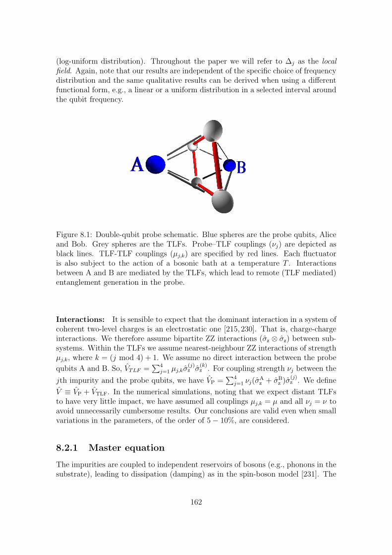
(log-uniform distribution). Throughout the paper we will refer to ∆j as the localfield. Again, note that our results are independent of the specific choice of frequencydistribution and the same qualitative results can be derived when using a differentfunctional form, e.g., a linear or a uniform distribution in a selected interval aroundthe qubit frequency.
Figure 8.1: Double-qubit probe schematic. Blue spheres are the probe qubits, Aliceand Bob. Grey spheres are the TLFs. Probe–TLF couplings (νj) are depicted asblack lines. TLF-TLF couplings (µj,k) are specified by red lines. Each fluctuatoris also subject to the action of a bosonic bath at a temperature T . Interactionsbetween A and B are mediated by the TLFs, which lead to remote (TLF mediated)entanglement generation in the probe.
Interactions: It is sensible to expect that the dominant interaction in a system ofcoherent two-level charges is an electrostatic one [215, 230]. That is, charge-chargeinteractions. We therefore assume bipartite ZZ interactions (σz ⊗ σz) between sub-systems. Within the TLFs we assume nearest-neighbour ZZ interactions of strengthµj,k, where k = (j mod 4) + 1. We assume no direct interaction between the probe
qubits A and B. So, VTLF =∑4
j=1 µj,kσ(j)z σ
(k)z . For coupling strength νj between the
jth impurity and the probe qubits, we have VP =∑4
j=1 νj(σAz + σB
z )σ(j)z . We define
V ≡ VP + VTLF. In the numerical simulations, noting that we expect distant TLFsto have very little impact, we have assumed all couplings µj,k = µ and all νj = ν toavoid unnecessarily cumbersome results. Our conclusions are valid even when smallvariations in the parameters, of the order of 5− 10%, are considered.
8.2.1 Master equation
The impurities are coupled to independent reservoirs of bosons (e.g., phonons in thesubstrate), leading to dissipation (damping) as in the spin-boson model [231]. The
162
Hamiltonians in the pseudo-spin basis are
Hsq =1
2Ωsz
HTLF =1
2
∑j
Ωj s(j)z
Vsq−TLF =∑
j
νj(cos θsz − sin θsx)(cos θj s(j)z − sin θj s
(j)x )
VTLF =∑
j,kµj,k(cos θj s
(j)z − sin θj s
(j)x )(cos θks
(k)z − sin θks
(k)x )
VTLF−B =∑
`,j
λ`(cos θj s(j)z − sin θj s
(j)x )
(a`,j + a†`,j
)
where tan θj ≡ ∆j/εj. In order to obtain a master equation we follow the simplest
approach explained in section 4.1.4, i.e. we assume again that the presence of Vsq−TLF
and VTLF do not disturb so much to the master equation obtained for independentfree “probe plus TLFs”, and these interactions terms affects only the Hamiltonianpart. Following then the weak coupling strategy we obtain the following Markovianmaster equation for the joint state ρ(t) of the probe plus impurities:
dρ(t)
dt= −i[H, ρ(t)] +
∑j(D(j)
z +D(j)+ +D(j)
− )ρ(t), (8.1)
where the total Hamiltonian is
H = HP + HTLF + V . (8.2)
The D superoperators represent decoherence in the TLFs due to coupling withthe bosonic baths, which are at temperature T . The decoherence consists of de-phasing D(j)
z ρ = Γ(j)z [s
(j)z ρs
(j)z − ρ], emission into the baths D(j)
− ρ = Γ(j)− [s
(j)− ρs
(j)+ −
(s(j)+ s
(j)− ρ + ρs
(j)+ s
(j)− )/2], and absorption from the baths D(j)
+ ρ = Γ(j)+ [s
(j)+ ρs
(j)− −
(s(j)− s
(j)+ ρ + ρs
(j)− s
(j)+ )/2]. The TLF decoherence rates are Γ
(j)z = γz cos2 θj/2, Γ
(j)− =
(γ− + γ+) sin2 θj/4 and Γ(j)+ = γ+ sin2 θj/4. Here γz, γ− and γ+ are the dephasing
rate, the spontaneous emission rate and stimulated emission rate respectively, whichcan be calculated by knowing the spectral properties and temperature of the bath.
To get a feel for the influence of the ratio tan θj ≡ ∆j/εj; if we assume dissipation-limited dephasing (γz = γ−/2) and sufficiently low temperature (γ+/γ− → 0), thentan θj dictates the dominance of pure dephasing or relaxation in each TLF. Specif-
ically, Γ(j)z /Γ
(j)− = 1/ tan2 θj so that pure dephasing dominates the TLF decoher-
ence for weak local fields, and relaxation dominates for strong local fields. Follow-ing [210], we distribute the random TLF parameters εj, ∆j, and γ
(j)z,± as per the
distributions P (εj) ∝ εj, P (∆j) ∝ 1/∆j, P (γ(j)z,±) ∝ 1/γ
(j)z,±. We choose these pa-
rameters to take values within the following moderate ranges: εj ∈ (1± 0.5)εj; ∆j
∈ ∆j ± 0.5 min(ΩP, ∆j); γ(j)z,± ∈ [Ωmin/6, Ωmin/2], where Ωmin is the minimum spin
163
frequency amongst the TLFs. We are free to select sensible values for the overbarquantities εj and ∆j, which we will reference to the tunable probe frequency ΩP.
We take the probe-TLF coupling to be uniform (νj = ν) and weak comparedwith all of the TLF frequencies: ν = Ωmin/3. To give an estimation of the validityof (8.1) under real conditions, weak probe-TLF coupling is in accord with the recentexperiments of [211, 212], as well as the experiment of [209] (see [214]) where νj ∼MHz and Ωj ∼ ΩP ∼ GHz. The TLF-TLF coupling is also assumed to be uniformµj,k = µ, and µ/ν is often believed to be small (see [224], for example).
8.2.2 Observable quantities
We restrict our knowledge to the probe subsystem (as would be the case in an exper-iment). A notable observable quantity on the probe is the magnetization, which isrelated to a simple sum of Pauli operators: Mx(t) = sA
x + sBx . The appeal of consid-
ering the probe magnetization is that it requires only tractable, local measurementson each probe qubit. That is, our results may be easily tested in an experiment.It is worth noting that a result of Audenaert and Plenio [229] shows that measur-ing correlations Cxx/zz = 〈σx/z ⊗ σx/z〉 along the XX and ZZ “directions” suffice togive a lower bound on the probe entanglement. This can remove the requirementfor full tomographic (entanglement) measurements when verifying or quantifyingentanglement in the probe.
The time series resulting from measuring the probe’s X-magnetization is M(t) =〈Mx(t)〉. The mean-square power spectrum of M(t) is given by
S(ω) =∫∞−∞ R(τ)e−iωτdτ, (8.3)
where the reduced auto-correlation function is R(τ) ≡ 〈M(t + τ)M(t)〉 − 〈M(t +τ)〉〈M(t)〉. R(t) is a discrete quantity (the data is a time series), and so the powerspectrum obtained is an estimate (the Fourier transform of the reduced autocor-relation of the time series M(t)). This estimate of average power as a function offrequency can theoretically be improved (by increasing the duration of the experi-ment, for example), but this may not be practical in reality.
8.3 Results: detecting the presence of coupling
between the TLFs
Can probe observables reveal the degree of connectivity of a composite spin-bosonenvironment? In this section we present numerical results showing that this isindeed the case. Observable quantities we consider are the probe magnetization, itsestimated power spectrum, and the remote entanglement between the probe qubits.Entanglement generated between probe qubits that are initially in a separable stateis primarily due to the structure of the spin-boson environment (e.g., the presenceor absence of TLF-TLF interactions in the surroundings of the probe).
164
Initially we set the probe to be in a state orthogonal to the sz eigen-axis:|ψP(0)〉 = |+〉A|+〉B. The TLFs are assumed to be initially in a zero-temperaturethermal state, i.e., the ground state of HTLF, which we denote as |g〉. So, |φTLF(0)〉 =|g〉. We plot observable quantities as a function of the ratio of TLF-TLF couplingstrength to probe-TLF coupling strength, µ/ν, which is often believed to be smallas we already said.
Section 8.3.1 considers the estimated power spectrum of 〈Mx(t)〉. Section 8.3.2considers the build up of entanglement in the probe.
8.3.1 Power spectrum of 〈Mx〉TLFs with weak local fields.
Consider the case of “weak” local fields in the spin-boson environment where tan θj ∼1/3 (specifically ∆j/εj = 1/3, where TLF dephasing dominates relaxation: Γz/Γ− ∼10). In our probing of TLF connectivity, we tune the ratio of probe–TLF splittingεP/εj to 10, 3 and 1, corresponding to figures 8.2(a), 8.2(b) and 8.2(c), respectively.We observe two effects: 1. For weaker TLF interconnectivity µ/ν . 0.6, a decrease isobserved in the height of the single dominant peak in the spectrum; 2. For strongerTLF interconnectivity µ/ν ≈ 1, the spectrum splits into multiple peaks, the mostdominant of which is shifted in frequency relative to µ/ν = 0. This is visible infigure 8.2 where the gold traces (µ/ν = 1) are the most qualitatively different fromthe blue traces (µ = 0). The power in the signal 〈Mx(t)〉 redistributes from onedominant frequency for unconnected TLFs (µ = 0), to multiple frequencies as µ/νapproaches unity (highly connected TLFs). Remarkably, the most dominant peakfor highly connected TLFs µ/ν = 1 is qualitatively similar to the case of an isolatedprobe (figure 8.2) — a single peak at ω = ΩP — although the peak visibility (height)is noticeably less than the isolated probe.
Effect of TLF local field.
Above we have established that we can distinguish between highly connected TLFs(µ = ν) and unconnected TLFs (µ = 0) for weak local field strength ∆j < εj. Itis interesting to ask how stronger local fields affect our ability to distinguish thesetwo values of µ. To explore this, we increase the ratio of TLF field strength to split-ting: tan θj = ∆j/εj, which was less than 1 in figure 8.2. This varies the range for∆j, which (we remind the reader) we have taken to be ∆j ± 0.5 min(∆j, ΩP). Thisrange ensures a sensible variation in the TLF local field strengths of no greater thanone-half of the probe frequency. We assume that the TLF energies are distributedover a relatively small range as might be expected for systematically formed impu-rities/defects.
As the local field increases tan θj > 1, two different effects occur: 1. Largerlocal fields cause relaxation to dominate over dephasing in the TLF decoherence;2. The TLF eigenstates increasingly align towards the σx axis, and seem to have adecreasing effect on the probe. Evidence to support this is shown in figure 8.3, which
165
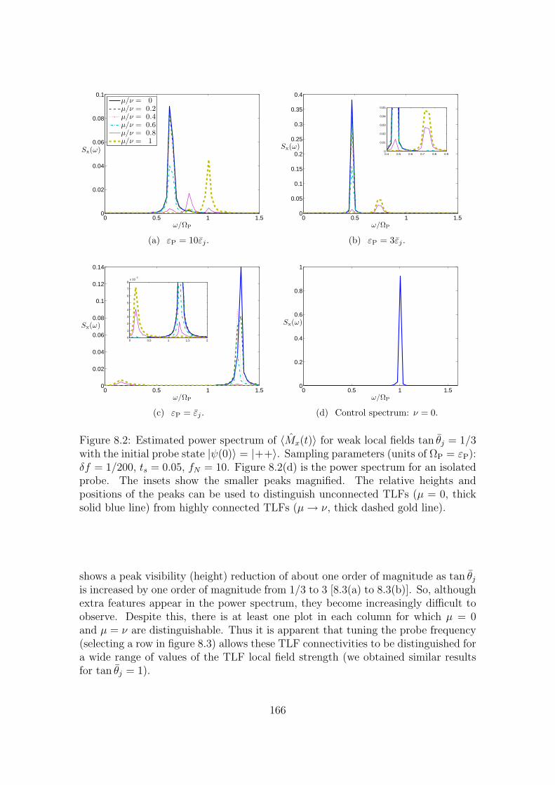
0 0.5 1 1.50
0.02
0.04
0.06
0.08
0.1
ω/ΩP
Sx(ω)
µ/ν = 0µ/ν = 0.2µ/ν = 0.4µ/ν = 0.6µ/ν = 0.8µ/ν = 1
(a) εP = 10εj .
0 0.5 1 1.50
0.05
0.1
0.15
0.2
0.25
0.3
0.35
0.4
ω/ΩP
Sx(ω)
0.4 0.5 0.6 0.7 0.8 0.90
0.01
0.02
0.03
0.04
0.05
(b) εP = 3εj .
0 0.5 1 1.50
0.02
0.04
0.06
0.08
0.1
0.12
0.14
ω/ΩP
Sx(ω)
0 0.5 1 1.5 20
1
2
3
4
5
6
7
8x 10
−3
(c) εP = εj .
0 0.5 1 1.50
0.2
0.4
0.6
0.8
1
ω/ΩP
Sx(ω)
(d) Control spectrum: ν = 0.
Figure 8.2: Estimated power spectrum of 〈Mx(t)〉 for weak local fields tan θj = 1/3with the initial probe state |ψ(0)〉 = |++〉. Sampling parameters (units of ΩP = εP):δf = 1/200, ts = 0.05, fN = 10. Figure 8.2(d) is the power spectrum for an isolatedprobe. The insets show the smaller peaks magnified. The relative heights andpositions of the peaks can be used to distinguish unconnected TLFs (µ = 0, thicksolid blue line) from highly connected TLFs (µ → ν, thick dashed gold line).
shows a peak visibility (height) reduction of about one order of magnitude as tan θj
is increased by one order of magnitude from 1/3 to 3 [8.3(a) to 8.3(b)]. So, althoughextra features appear in the power spectrum, they become increasingly difficult toobserve. Despite this, there is at least one plot in each column for which µ = 0and µ = ν are distinguishable. Thus it is apparent that tuning the probe frequency(selecting a row in figure 8.3) allows these TLF connectivities to be distinguished fora wide range of values of the TLF local field strength (we obtained similar resultsfor tan θj = 1).
166
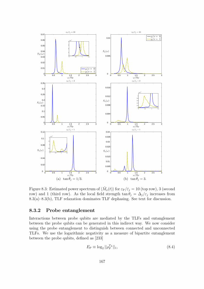
0 0.5 1 1.5 2 2.5 30
0.01
0.02
0.03
0.04
0.05
0.06
0.07εP/εj = 10
ω/ΩP
µ/ν = 0µ/ν = 1
0 0.5 1 1.50
1
2
3
4x 10
−3
SX(ω)
0 0.5 1 1.5 2 2.5 30
0.05
0.1
0.15
0.2
0.25
0.3
0.35εP/εj = 3
ω/ΩP
Sx(ω)
0 0.5 1 1.5 2 2.5 30
0.02
0.04
0.08
0.1
0.12εP/εj = 1
ω/ΩP
Sx(ω)
0 0.5 1 1.50
0.5
1
1.5
2x 10
−3
(a) tan θj = 1/3.
0 0.5 1 1.5 2 2.5 30
0.005
0.01
εP/εj = 10
ω/ΩP
Sx(ω)
µ/ν = 0µ/ν = 1
0 0.5 1 1.5 2 2.5 30
0.004
0.008
0.012
0.016
εP/εj = 3
ω/ΩP
Sx(ω)
0 0.5 1 1.50
0.2
0.4
0.6
0.8
1
x 10−3
0 0.5 1 1.5 2 2.5 30
0.005
0.01
0.015
0.025
0.03
0.035
0.04 εP/εj = 1
ω/ΩP
Sx(ω)
(b) tan θj = 3.
Figure 8.3: Estimated power spectrum of 〈Mx(t)〉 for εP/εj = 10 (top row), 3 (secondrow) and 1 (third row). As the local field strength tan θj = ∆j/εj increases from8.3(a)–8.3(b), TLF relaxation dominates TLF dephasing. See text for discussion.
8.3.2 Probe entanglement
Interactions between probe qubits are mediated by the TLFs and entanglementbetween the probe qubits can be generated in this indirect way. We now considerusing the probe entanglement to distinguish between connected and unconnectedTLFs. We use the logarithmic negativity as a measure of bipartite entanglementbetween the probe qubits, defined as [233]
EP ≡ log2 ||ρTAP ||1, (8.4)
167
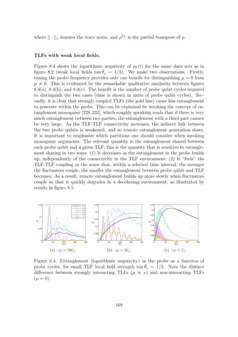
where || · ||1 denotes the trace norm, and ρTA is the partial transpose of ρ.
TLFs with weak local fields.
Figure 8.4 shows the logarithmic negativity of ρP(t) for the same data sets as infigure 8.2 (weak local fields tan θj = 1/3). We make two observations. Firstly,tuning the probe frequency provides only one benefit for distinguishing µ = 0 fromµ 6= 0. This is evidenced by the remarkable qualitative similarity between figures8.4(a), 8.4(b), and 8.4(c). The benefit is the number of probe qubit cycles requiredto distinguish the two cases (time is shown in units of probe qubit cycles). Sec-ondly, it is clear that strongly coupled TLFs (the gold line) cause less entanglementto generate within the probe. This can be explained by invoking the concept of en-tanglement monogamy [228,232], which roughly speaking reads that if there is verymuch entanglement between two parties, the entanglement with a third part cannotbe very large. As the TLF-TLF connectivity increases, the indirect link betweenthe two probe qubits is weakened, and so remote entanglement generation slows.It is important to emphasize which partitions one should consider when invokingmonogamy arguments. The relevant quantity is the entanglement shared betweeneach probe qubit and a given TLF; this is the quantity that is sensitive to entangle-ment sharing in two ways: (1) It decreases as the entanglement in the probe buildsup, independently of the connectivity in the TLF environment; (2) It “feels” theTLF-TLF coupling in the sense that, within a selected time interval, the strongerthe fluctuators couple, the smaller the entanglement between probe qubit and TLFbecomes. As a result, remote entanglement builds up more slowly when fluctuatorscouple so that it quickly degrades in a decohering environment, as illustrated byresults in figure 8.5.
0 50 100 150 2000
0.05
0.1
0.15
ΩPt
EP
µ/ν = 0
µ/ν = 0.2
µ/ν = 0.4
µ/ν = 0.6
µ/ν = 0.8
µ/ν = 1
(a) εP = 10εj .
0 50 100 150 2000
0.05
0.1
0.15
0.2
0.25
ΩPt
EP
(b) εP = 3εj .
0 50 100 150 2000
0.05
0.1
0.15
0.2
0.25
0.3
0.35
ΩPt
EP
(c) εP = εj .
Figure 8.4: Entanglement (logarithmic negativity) in the probe as a function ofprobe cycles, for small TLF local field strength tan θj = 1/3. Note the distinctdifference between strongly interacting TLFs (µ ≈ ν) and non-interacting TLFs(µ = 0).
168
Effect of the TLF local field.
Unlike the power spectrum (figure 8.3), the probe entanglement EP(t) remains usefulfor distinguishing µ = 0 from µ 6= 0 for strong local fields in the TLFs where tan θj >1. Figure 8.5 shows the probe entanglement as a function of time for the same datasets as in figure 8.3. It is clear that entanglement is generated within the probe forsome time, before the TLF decoherence causes it to dissipate. As argued before,this loss of generated probe entanglement occurs faster for highly connected TLFswith µ/ν = 1, as one might expect, even without no explicit mention of monogamyconstraints, since these TLF-TLF connections provide more links between the probequbits and the TLF decoherence channels. This faster dissipation of generatedentanglement for highly-connected TLFs allows us to distinguish between µ/ν = 0and µ/ν = 1 after 10 to 50 probe qubit cycles, depending on the TLF parameters.Similar conclusions can be drawn for tan θj = 1.
8.3.3 Discussion of the results
Since we are performing local measurements on each probe qubit, one might askif there are any advantages of using a double-qubit probe. An obvious advantageis that entanglement within the probe becomes an accessible quantity that is notpossible in a single-qubit probe. This is important for detecting the TLF-TLFconnectivity, as we have seen that this task was achievable over a wider range ofTLF parameters using the probe entanglement than the power spectra of the probemagnetization (which yielded qualitatively similar results for both types of probes).
In section 8.3 we were able to distinguish between composite spin-boson envi-ronments with high connectivity from those with low connectivity. The param-eter ranges for which our findings were robust are: εP/εj = 1, 3, 10 (tunable),1/3 ≤ tan θj ≤ 3. Other parameters (Γ, etc) are restricted to lie within the rangesthat ensure validity of the master equation (8.1).
For all numerical calculations in this paper we have assumed effectively zero-temperature bosonic baths where nj = [exp(~Ωj/kBT ) − 1]−1 ¿ 1. The relevantfrequencies for experiments with Josephson qubits are in the vicinity of 10 GHz[209, 211, 212, 234], with cryostat temperatures of the order of 30 mK [209]. Thesevalues give n ∼ 0.1, so the low-temperature approximation is good.
In general, determining the probe entanglement would require full quantum-statetomography. Here we consider estimating the probe entanglement from measure-ments less costly than full quantum state tomography, as described in [229] (andreferences within). The result is lower bounds on the entanglement — we refer thereader to [229] for details.
For all parameter regimes considered in this paper we found that one of the lowerbounds given in [229] — the optimal one given in (8.5) — provided a remarkablygood approximation to the probe entanglement for all times. The other lower boundsC1,2 in [229] did not approximate the probe entanglement well for any time. Anexample is shown in figure 8.6. The solid line is the entanglement within the probe
169
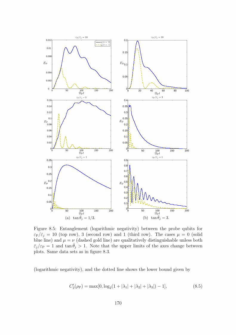
0 50 100 150 2000
0.002
0.004
0.008
0.01
0.012εP/εj = 10
ΩPt
EP
µ/ν = 0
µ/ν = 1
0 50 100 150 2000
0.02
0.04
0.06
0.08
0.1
0.12
0.14
0.16εP/εj = 3
ΩPt
EP
0 50 100 150 2000
0.05
0.1
0.15
0.2
0.25
0.3
0.35εP/εj = 1
ΩPt
EP
(a) tan θj = 1/3.
0 20 40 60 80 1000
0.05
0.1
0.15
0.2εP/εj = 10
ΩPt
EP
0 50 100 150 2000
0.05
0.1
0.15
0.2
0.25
0.3
0.35
0.4εP/εj = 3
ΩPt
EP
0 50 100 150 2000
0.1
0.2
0.3
0.4
0.5
0.6
0.7
0.8
0.9εP/εj = 1
ΩPt
EP
(b) tan θj = 3.
Figure 8.5: Entanglement (logarithmic negativity) between the probe qubits forεP/εj = 10 (top row), 3 (second row) and 1 (third row). The cases µ = 0 (solidblue line) and µ = ν (dashed gold line) are qualitatively distinguishable unless bothεj/εP = 1 and tan θj > 1. Note that the upper limits of the axes change betweenplots. Same data sets as in figure 8.3.
(logarithmic negativity), and the dotted line shows the lower bound given by
C ′2(ρP) = max[0, log2(1 + |λ1|+ |λ2|+ |λ3|)− 1], (8.5)
170
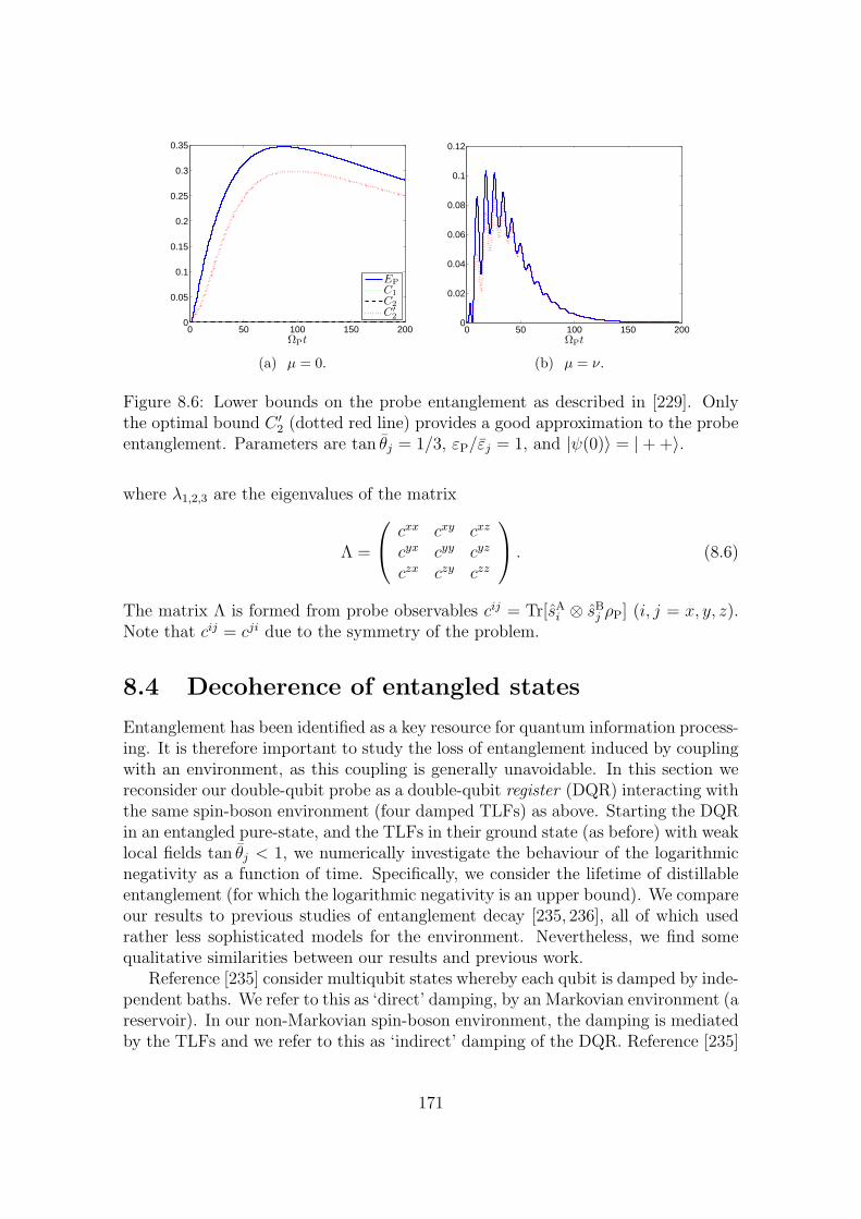
0 50 100 150 2000
0.05
0.1
0.15
0.2
0.25
0.3
0.35
ΩPt
EP
C1
C2
C′
2
(a) µ = 0.
0 50 100 150 2000
0.02
0.04
0.06
0.08
0.1
0.12
ΩPt
(b) µ = ν.
Figure 8.6: Lower bounds on the probe entanglement as described in [229]. Onlythe optimal bound C ′
2 (dotted red line) provides a good approximation to the probeentanglement. Parameters are tan θj = 1/3, εP/εj = 1, and |ψ(0)〉 = |+ +〉.
where λ1,2,3 are the eigenvalues of the matrix
Λ =
cxx cxy cxz
cyx cyy cyz
czx czy czz
. (8.6)
The matrix Λ is formed from probe observables cij = Tr[sAi ⊗ sB
j ρP] (i, j = x, y, z).Note that cij = cji due to the symmetry of the problem.
8.4 Decoherence of entangled states
Entanglement has been identified as a key resource for quantum information process-ing. It is therefore important to study the loss of entanglement induced by couplingwith an environment, as this coupling is generally unavoidable. In this section wereconsider our double-qubit probe as a double-qubit register (DQR) interacting withthe same spin-boson environment (four damped TLFs) as above. Starting the DQRin an entangled pure-state, and the TLFs in their ground state (as before) with weaklocal fields tan θj < 1, we numerically investigate the behaviour of the logarithmicnegativity as a function of time. Specifically, we consider the lifetime of distillableentanglement (for which the logarithmic negativity is an upper bound). We compareour results to previous studies of entanglement decay [235, 236], all of which usedrather less sophisticated models for the environment. Nevertheless, we find somequalitative similarities between our results and previous work.
Reference [235] consider multiqubit states whereby each qubit is damped by inde-pendent baths. We refer to this as ‘direct’ damping, by an Markovian environment (areservoir). In our non-Markovian spin-boson environment, the damping is mediatedby the TLFs and we refer to this as ‘indirect’ damping of the DQR. Reference [235]
171
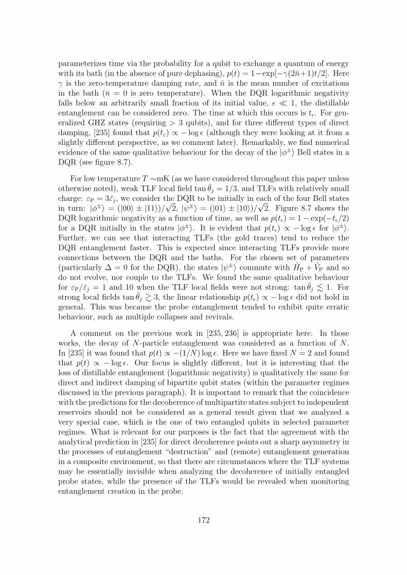
parameterizes time via the probability for a qubit to exchange a quantum of energywith its bath (in the absence of pure dephasing), p(t) = 1−exp[−γ(2n+1)t/2]. Hereγ is the zero-temperature damping rate, and n is the mean number of excitationsin the bath (n = 0 is zero temperature). When the DQR logarithmic negativityfalls below an arbitrarily small fraction of its initial value, ε ¿ 1, the distillableentanglement can be considered zero. The time at which this occurs is tε. For gen-eralized GHZ states (requiring > 3 qubits), and for three different types of directdamping, [235] found that p(tε) ∝ − log ε (although they were looking at it from aslightly different perspective, as we comment later). Remarkably, we find numericalevidence of the same qualitative behaviour for the decay of the |φ±〉 Bell states in aDQR (see figure 8.7).
For low temperature T ∼mK (as we have considered throughout this paper unlessotherwise noted), weak TLF local field tan θj = 1/3, and TLFs with relatively smallcharge: εP = 3εj, we consider the DQR to be initially in each of the four Bell statesin turn: |φ±〉 = (|00〉 ± |11〉)/√2, |ψ±〉 = (|01〉 ± |10〉)/√2. Figure 8.7 shows theDQR logarithmic negativity as a function of time, as well as p(tε) = 1− exp(−tε/2)for a DQR initially in the states |φ±〉. It is evident that p(tε) ∝ − log ε for |φ±〉.Further, we can see that interacting TLFs (the gold traces) tend to reduce theDQR entanglement faster. This is expected since interacting TLFs provide moreconnections between the DQR and the baths. For the chosen set of parameters(particularly ∆ = 0 for the DQR), the states |ψ±〉 commute with HP + VP and sodo not evolve, nor couple to the TLFs. We found the same qualitative behaviourfor εP/εj = 1 and 10 when the TLF local fields were not strong: tan θj . 1. Forstrong local fields tan θj & 3, the linear relationship p(tε) ∝ − log ε did not hold ingeneral. This was because the probe entanglement tended to exhibit quite erraticbehaviour, such as multiple collapses and revivals.
A comment on the previous work in [235, 236] is appropriate here. In thoseworks, the decay of N -particle entanglement was considered as a function of N .In [235] it was found that p(t) ∝ −(1/N) log ε. Here we have fixed N = 2 and foundthat p(t) ∝ − log ε. Our focus is slightly different, but it is interesting that theloss of distillable entanglement (logarithmic negativity) is qualitatively the same fordirect and indirect damping of bipartite qubit states (within the parameter regimesdiscussed in the previous paragraph). It is important to remark that the coincidencewith the predictions for the decoherence of multipartite states subject to independentreservoirs should not be considered as a general result given that we analyzed avery special case, which is the one of two entangled qubits in selected parameterregimes. What is relevant for our purposes is the fact that the agreement with theanalytical prediction in [235] for direct decoherence points out a sharp asymmetry inthe processes of entanglement “destruction” and (remote) entanglement generationin a composite environment, so that there are circumstances where the TLF systemsmay be essentially invisible when analyzing the decoherence of initially entangledprobe states, while the presence of the TLFs would be revealed when monitoringentanglement creation in the probe.
172
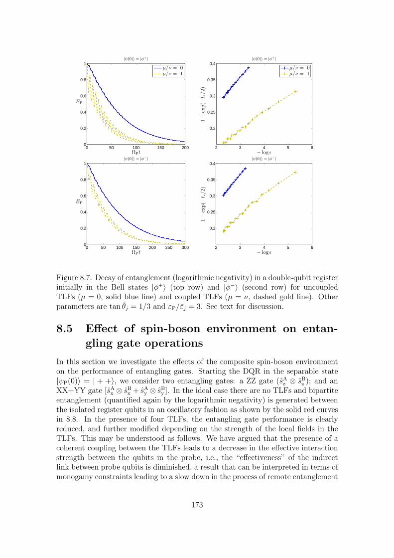
0 50 100 150 2000
0.2
0.4
0.6
0.8
1|ψ(0)〉 = |φ+〉
ΩPt
EP
µ/ν = 0µ/ν = 1
2 3 4 5 6
0.2
0.25
0.3
0.35
0.4|ψ(0)〉 = |φ+〉
1−
exp(−t ε/2)
− log ε
µ/ν = 0µ/ν = 1
0 50 100 150 200 250 3000
0.2
0.4
0.6
0.8
1|ψ(0)〉 = |φ−〉
ΩPt
EP
2 3 4 5 6
0.2
0.25
0.3
0.35
0.4|ψ(0)〉 = |φ−〉
1−
exp(−t ε/2)
− log ε
Figure 8.7: Decay of entanglement (logarithmic negativity) in a double-qubit registerinitially in the Bell states |φ+〉 (top row) and |φ−〉 (second row) for uncoupledTLFs (µ = 0, solid blue line) and coupled TLFs (µ = ν, dashed gold line). Otherparameters are tan θj = 1/3 and εP/εj = 3. See text for discussion.
8.5 Effect of spin-boson environment on entan-
gling gate operations
In this section we investigate the effects of the composite spin-boson environmenton the performance of entangling gates. Starting the DQR in the separable state|ψP(0)〉 = | + +〉, we consider two entangling gates: a ZZ gate (sA
z ⊗ sBz ); and an
XX+YY gate [sAx ⊗ sB
x + sAy ⊗ sB
y ]. In the ideal case there are no TLFs and bipartiteentanglement (quantified again by the logarithmic negativity) is generated betweenthe isolated register qubits in an oscillatory fashion as shown by the solid red curvesin 8.8. In the presence of four TLFs, the entangling gate performance is clearlyreduced, and further modified depending on the strength of the local fields in theTLFs. This may be understood as follows. We have argued that the presence of acoherent coupling between the TLFs leads to a decrease in the effective interactionstrength between the qubits in the probe, i.e., the “effectiveness” of the indirectlink between probe qubits is diminished, a result that can be interpreted in terms ofmonogamy constraints leading to a slow down in the process of remote entanglement
173
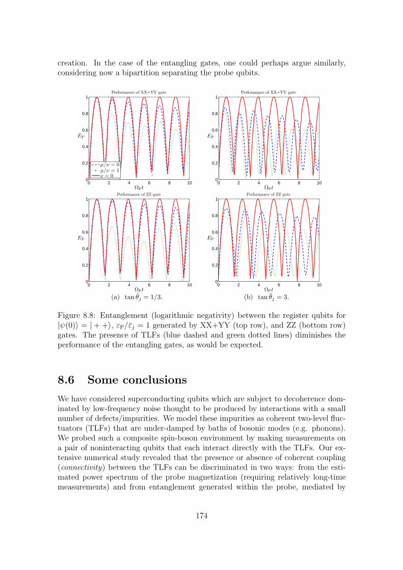
creation. In the case of the entangling gates, one could perhaps argue similarly,considering now a bipartition separating the probe qubits.
0 2 4 6 8 100
0.2
0.4
0.6
0.8
1Performance of XX+YY gate
ΩPt
EP
µ/ν = 0µ/ν = 1ν = 0
0 2 4 6 8 100
0.2
0.4
0.6
0.8
1Performance of ZZ gate
ΩPt
EP
(a) tan θj = 1/3.
0 2 4 6 8 100
0.2
0.4
0.6
0.8
1Performance of XX+YY gate
ΩPt
EP
0 2 4 6 8 100
0.2
0.4
0.6
0.8
1Performance of ZZ gate
ΩPt
EP
(b) tan θj = 3.
Figure 8.8: Entanglement (logarithmic negativity) between the register qubits for|ψ(0)〉 = | + +〉, εP/εj = 1 generated by XX+YY (top row), and ZZ (bottom row)gates. The presence of TLFs (blue dashed and green dotted lines) diminishes theperformance of the entangling gates, as would be expected.
8.6 Some conclusions
We have considered superconducting qubits which are subject to decoherence dom-inated by low-frequency noise thought to be produced by interactions with a smallnumber of defects/impurities. We model these impurities as coherent two-level fluc-tuators (TLFs) that are under-damped by baths of bosonic modes (e.g. phonons).We probed such a composite spin-boson environment by making measurements ona pair of noninteracting qubits that each interact directly with the TLFs. Our ex-tensive numerical study revealed that the presence or absence of coherent coupling(connectivity) between the TLFs can be discriminated in two ways: from the esti-mated power spectrum of the probe magnetization (requiring relatively long-timemeasurements) and from entanglement generated within the probe, mediated by
174
the spin-boson environment. We argue that entanglement monogamy considera-tions [228] allow interpretation of our results in terms of an effective decrease in theremote interaction strength when the environment is connected, which yields to acreation of quantum correlations on a much larger time scale as compared with theuncoupled fluctuator case.
We also showed that this remotely generated entanglement can be well-estimatedby a lower bound [229] that requires less experimental effort than the full quantumstate tomography required to evaluate the entanglement. The upshot is that thisconnectivity of the TLFs should be discernible using tractable measurements in areal experiment. This result is important for studies of quantum-mechanical phe-nomena in Josephson devices (including quantum computing) where it is desirableto minimize the effects of decoherence, for which the TLF-TLF connectivity mayplay a significant role [222].
When considering the effects of the spin-boson environment on a double-qubitregister initially prepared in a maximally-entangled (Bell) state, we showed that thepresence of TLFs may be unnoticeable in certain parameter regimes, in the sensethat entanglement degradation there is well approximated by the same decrease lawas for direct decoherence. This fact emphasizes the possible usefulness of monitoringthe reverse process of entanglement generation for environmental probing.
The presence of TLF-TLF coupling also showed a reduction in the performanceof entangling gate operations performed on the register.
175

Chapter 9
Mapping reservoirs to semi-infinitediscrete chains
9.1 Introduction
The theoretical description of a quantum system coupled to environmental degreesof freedom has been developed over many decades, and of particular important inthese studies is the spin-boson model (SBM) [15, 231], one of the simplest non-trivial models of open-system dynamics. This model describes a single two-levelsystem (TLS) coupled linearly to the coordinates of an environment consisting ofa continuum of harmonic oscillators. Despite its simplicity, this model cannot besolved exactly and shows a rich array of non-Markovian dynamical phenomena,including a type of quantum phase transition between dynamically localized anddelocalized states of the TLS for so-called Ohmic and sub-Ohmic baths at zerotemperature [111,112,231,237–241]. These interesting dynamics normally appear insituations where the effective interaction between the TLS and the oscillators cannotbe treated perturbatively, and although many analytical and formal approaches haveshed considerable light on the nature of the effects, the explicit time evolution of theTLS in these regimes must normally be simulated numerically. These simulationscan be loosely divided into methods in which the environmental degrees of freedomare eliminated in order to derive an effective equation of motion for the TLS, andthose in which the complete many-body dynamics of the TLS and the environmentare computed. The former approach includes the hierarchy approach [242] andvarious numerical path integral techniques [243], while the latter includes exactdiagonalization and the numerical reorganization group (NRG) approaches [244].
Recently, the time-adaptive density matrix renormalisation group (t-DMRG)[245] has also been added to this category. This approach provides numerically-exact simulations for the dynamics of one-dimensional systems with short-rangeinteractions, and is regarded as one of the most powerful and versatile methods incondensed matter, atomic, and optical physics for the study of strongly-correlatedmany-body quantum states. The recent study of Prior et al. [113] successfully useda t-DMRG approach for a two-spin system where each spin was in contact with
177
an oscillator environment with arbitrarily complex spectral densities. The imple-mentation and accuracy of this approach rests on an exact mapping between thecanonical SBM and a one-dimensional harmonic chain with short range interactions.The reasons why this form of Hamiltonian allows the t-DMRG to efficiently simulateextremely large chains is discussed at length in Ref. [245].
The idea of this mapping was first introduced in the NRG studies of Bulla etal. [111, 112, 241], who first discretise the continuous environment and then per-form a recursive numerical technique to bring the truncated finite Hamiltonian tothe desired chain form. The dynamics of this chain can then be numerically simu-lated [246]. In addition, lately, Martinazzo et al. [247] have also proposed a recursiveapproach to this kind of transformation for the case a Brownian particle. In thischapter we show how the formal properties of orthogonal polynomials can be usedto implement an exact unitary transformation which maps an arbitrary continuousSBM directly onto the nearest-neighbors 1−D chain without any need for discreti-sation. In several important cases we can actually perform the mapping analyticallyand predict the energies and couplings of the chain in closed form. Our analysisof the mapping shows that these energies and couplings are simply related to therecurrence coefficients of orthogonal polynomials, and when analytical results arenot available, we can make use of sophisticated numerical techniques that computerecurrence coefficients with high precision and which do not suffer from the nu-merical instabilities which often appear in the standard recursive technique. Notonly does this transformation aid the simulation of non-perturbative open-systemdynamics, we shall show that the use of orthogonal polynomials also reveals someuniversal features of TLS dynamics which are independent of the spectral density ofthe environmental oscillators, and which may point the way to even more efficientsimulations of strongly non-Markovian open-system dynamics.
The plan of this chapter is as follows. In section 9.2 we introduce the formalproperties of orthogonal polynomials needed to implement the chain mapping, andin section 9.3 we introduce the general model of an open quantum system whichcan be mapped onto a 1 − D chain suitable for t-DMRG simulation. This sectionalso contains details about the transformation itself and analytical expressions forthe frequencies and nearest-neighbors interactions of the chain are presented anddiscussed. Section 9.4 gives explicit examples of this transformation for the SBM,and 9.4.2 deals with an extension of the orthogonal polynomial method to systemsinteracting with a discrete number of environmental modes. These discrete envi-ronments may be found in certain physical systems, and are also important in theNRG description of open quantum systems where the continuous spectrum of theenvironment is approximated by a discrete set of oscillators [111,112,241]. We thenend with some general conclusions and a brief recapitulation of the main results.
178
9.2 Orthogonal polynomials
In this section we present a few useful properties of orthogonal polynomials thatwill be employed in the following. This section also serves to fix our notation.
9.2.1 Basic concepts
Let P be the space of the polynomials with real coefficients (the following may alsobe extended to complex, but real coefficients will be enough for our proposes), andPn ⊂ P the space of polynomials of degree equal to n, this is pn(x) ∈ Pn:
pn(x) =n∑
m=0
amxm,
where the am ∈ R and x is a real variable.
9.2.1. Definition. A polynomial pn(x) ∈ Pn is called monic if its leading coeffi-cient satisfies an = 1, will be denoted by pn(x) ≡ πn(x). Of course every polynomialof Pn can become monic just dividing it by an.
9.2.2. Definition. Let µ(x) be a nondecreasing and differentiable function onsome interval [a, b] ∈ R, and assume that the induced positive measure dµ(x) hasfinite moments of all orders:
∫ b
a
xrdµ(x) < ∞, r = 0, 1, 2, . . .
Then for any p(x), q(x) ∈ P we define an inner product as
〈p, q〉µ =
∫ b
a
p(x)q(x)dµ(x).
Of course it defines a norm via
‖p‖µ =√〈p, p〉µ =
(∫ b
a
p2(x)dµ(x)
)1/2
≥ 0,
and satisfies the Cauchy-Schwarz’s inequality,
|〈p, q〉µ| ≤ ‖p‖µ‖q‖µ.
9.2.3. Definition. Two polynomials p(x), q(x) ∈ P are said to be orthogonal withrespect to the measure dµ(x) if its inner product is zero 〈p, q〉µ = 0.
9.2.4. Definition. A set of monic polynomials πn(x) ∈ Pn, n = 0, 1, 2, . . . iscalled an orthogonal set with respect to the measure dµ(x) if
〈πn, πm〉µ = ‖πn‖2µδn,m for n,m = 0, 1, 2, . . .
Sometimes it is useful to normalize the monic polynomials, pn(x) = πn(x)/‖πn(x)‖µ,such that 〈pn, pm〉µ = δn,m, then the set is called orthonormal, however note that ingeneral the normalized polynomials lose the monic character.
179
9.2.5. Theorem. For any (non-zero) measure dµ(x) there exist a unique family ofmonic orthogonal polynomials πn(x) ∈ Pn, n = 0, 1, 2, . . ..
Proof. The proof is by construction. Applying the well-known Gram-Schmidt or-thogonalization procedure to the sequence 1, x, x2, . . ., the monic orthogonal poly-nomials are constructed from π0 = 1 using the formula:
πk(x) = mk(x)−k−1∑n=0
(〈mk, πn〉µ〈πn, πn〉µ
)πn,
with mk(x) = xk. 2
9.2.6. Theorem. The set of monic polynomials πn(x) ∈ Pn, n = 0, 1, 2, . . . is abasis of the space P. More specifically if p(x) is a polynomial of degree less or equalto r, then it can be uniquely represented by
p(x) =r∑
n=0
cnπn(x), (9.1)
for some real constants ck.
Proof. The proof is by mathematical induction. If r = 0 the proof is trivial.Assume that the statement is true for r − 1, then there is a unique cr such thatp(x)− crπr(x) = pr−1(x) is polynomial with degree less or equal to r− 1. Moreover,if the set of monic polynomials is orthogonal, taking the inner product on (9.1) withrespect to πm(x) we obtain
cn =〈πn, p〉µ‖πn‖2
µ
.
2
There are of course many more properties like these which are similar to thosefound in linear algebra spaces; however we are not going to go further in this wayhere, though the reader can find more information in references [248–250] for exam-ple. From now on we omit the subindex µ in the inner product and norms in orderto make the notation less dense.
9.2.2 Recurrence relations
One of the most useful properties for our interests is the recurrence formula ofthe orthogonal polynomials. Here we divide the section into two cases, monic andorthonormal polynomials.
180
9.2.7. Theorem. Let πn(x) ∈ Pn, n = 0, 1, 2, . . . be the set of monic orthogonalpolynomials with respect to some measure dµ(x), then
πk+1(x) = (x− αk)πk(x)− βkπk−1(x), k = 0, 1, 2... (9.2)
where π−1(x) ≡ 0, and the recurrence coefficients are:
αk =〈xπk, πk〉〈πk, πk〉 , βk =
〈πk, πk〉〈πk−1, πk−1〉 . (9.3)
Proof. By theorem 9.2.6, πk+1(x)− xπk(x) is a polynomial of degree less or equalto k, we can write it in terms of monic polynomials of degree less or equal k:
πk+1(x)− xπk(x) =k∑
n=0
cnπn(x),
and since the set is orthogonal
ck =〈πk+1 − xπk, πk〉
〈πk, πk〉 = −〈xπk, πk〉〈πk, πk〉 ,
similarly
ck−1 =〈πk+1 − xπk, πk−1〉〈πk−1, πk−1〉 = − 〈xπk, πk−1〉
〈πk−1, πk−1〉 = − 〈πk, xπk−1〉〈πk−1, πk−1〉 = − 〈πk, πk〉
〈πk−1, πk−1〉 ,
where in the last step we have used the fact that terms of degree less than k areorthogonal to πk(x), because they can be expressed as linear combination of πn(x) ∈Pn, n = 0, 1, 2, . . . , k− 1 which are all orthogonal to πk(x). By the same argument,it is easy to see that the remaining coefficients are zero cn = 0 for n = 0, . . . , k − 2.So by comparing with equation (9.2) we obtain αk = −ck and βk = −ck−1.
2
9.2.8. Theorem. Assume that we have a set of orthonormal polynomials pn(x) ∈Pn, n = 0, 1, 2, . . . then, the recurrence relation is:
pk+1(x) = (Ckx− Ak)pk(x)−Bkpk−1(x), k = 0, 1, 2... (9.4)
where p−1(x) ≡ 0. If we denote by κn the leading coefficient of pn(x) and by κ′n thesecond leading coefficient, i.e. pn(x) = κnx
n + κ′nxn−1 + . . ., we get
Ak =κk+1
κk
(κ′kκk
− κ′k+1
κk+1
), Bk =
κk+1κk−1
κ2k
, Ck =κk+1
κk
. (9.5)
181
Proof. The proof is not more complicated than in the monic case, if we choseCk = κk+1
κkthen, pk+1(x) − Ckxpk(x) is a polynomial of degree lower of equal to k,
in the same fashion the choice
Ak =Ckκ
′k − κ′k+1
κk
=κk+1
κk
(κ′kκk
− κ′k+1
κk+1
)
makes pk+1(x)− (Ckx−Ak)pk(x) a polynomial of degree lower of equal to k− 1. Byorthogonality the inner product of it with pn for n ≤ k − 2 are zero, and the innerproduct with pk−1 yields
〈pk−1, pk+1 − (Ckxpk + Ak)pk〉 = −Ck〈pk−1, xpk〉 = −Ck〈xpk−1, pk〉= −Ck
κk−1
κk
〈pk, pk〉 = −Ckκk−1
κk
,
so by taking into account that this is the coefficient which goes with pk−1, replacingthe value of Ck gives the value of Bk in (9.5). 2
The relation between both cases is given by the next proposition.
9.2.9. Proposition. Let πn(x) ∈ Pn, n = 0, 1, 2, . . . a set of monic orthogonalpolynomials and pn(x) = πn(x)/‖πn(x)‖ their orthonomalized version, then the co-efficients for the respective recurrence relations are related by:
Ak =αk√βk+1
, Bk =
√βk
βk+1
and Ck =1√βk+1
. (9.6)
Proof. Inserting πn(x) = ‖πn(x)‖pn(x) in (9.2) and dividing by ‖πk+1‖ one obtains
pk+1(x) =‖πk(x)‖‖πk+1(x)‖(x− αk)pk(x)− ‖πk−1(x)‖
‖πk+1(x)‖ pk−1(x).
Employing βk = ‖πk‖2/‖πk−1‖2 and comparing with the above (9.4) we obtain (9.6).2
9.2.3 Boundness properties of the recurrence coefficients
A particular important property for our work will be the behavior of the monic re-currence coefficients αn and βn when n is increasing. To start, we have the followingtheorem.
9.2.10. Theorem. Let the support interval [a, b] of dµ(x) be finite, then for eachk = 0, 1, 2, . . .
a ≤ αk ≤ b,
βk ≤ maxa2, b2.
182
Proof. The first relation follows immediately from αk = 〈xπk,πk〉〈πk,πk〉 because π2
k(x) ispositive for every x and a ≤ x ≤ b inside of the integration domain. For the secondrelation we have by orthogonality
〈πk, πk〉 = 〈xπk−1, πk〉,and the Cauchy-Schwarz’s inequality gives
〈πk, πk〉 ≤ |x|‖πk−1‖‖πk‖ ≤ max|a|, |b|‖πk−1‖‖πk‖,finally the division of both sides by ‖πk‖ and ‖πk−1‖ and squaring leads straightfor-wardly to the second bound. 2
Note that for measures with unbounded support, the monic recurrence coeffi-cients are not bounded as n increases; see for example the case of Laguerre andHermite polynomials [251]. However, for measures with bounded support furtheruseful properties about the recurrence coefficients can be obtained, to do this weneed the following results.
9.2.11. Proposition. Let πn(x) ∈ Pn, n = 0, 1, 2, . . . be a set of monic orthonor-mal polynomials with respect to some measure dµ(x) supported in [−1, 1], with re-cursion coefficients αk and βk defined according to (9.3). If we change the supportof the measure to [a, b] by means of a linear transformation y = mx + c, where
m =b− a
2, c =
a + b
2, (9.7)
the recursion coefficients α′k and β′k of the transformed monic polynomials π′n(y)∈ Pn, n = 0, 1, 2, . . . are given by
α′k = mαk + c, β′k = m2βk. (9.8)
Proof. The map y = mx + c transforms the measure dµ(y) = mdµ(x) andevery monic polynomial πk(x) = πk(
y−cm
) which is not a monic polynomial in y. Tomake these polynomials monic in y, we need to multiply by mk, that is, the set oftransformed monic polynomials is π′n(y) = mkπk(x) ∈ Pn, n = 0, 1, 2, . . .. Thenwe apply the definitions (9.3)
α′k =〈yπ′k, π
′k〉
〈π′k, π′k〉=
(m〈xπ′k, π′k〉+ c〈π′k, π′k〉)〈π′k, π′k〉
=m2k+1 (m〈xπk, πk〉+ c〈πk, πk〉)
m2k+1〈πk, πk〉 = mαk + c,
and similarly
β′k =〈π′k, π′k〉
〈π′k−1, π′k−1〉
=m2k+1〈πk, πk〉
m2(k−1)+1〈πk−1, πk−1〉 = m2βk.
2
183
9.2.12. Definition. A measure dµ(x) = w(x)dx supported in [−1, 1] belongs tothe Szego class if ∫ 1
−1
ln w(x)√1− x2
dx > −∞. (9.9)
9.2.13. Theorem (Szego). Let pn(x) ∈ Pn, n = 0, 1, 2, . . . orthonormal poly-nomials with respect to some Szego class measure dµ(x) = w(x)dx, then in theasymptotic limit n → ∞ we have the approximate expressions for the first leadingcoefficient κn and for the second one κ′n,
κn ' 2n
√π
exp
[− 1
2π
∫ 1
−1
ln w(x)√1− x2
dx
], (9.10)
κ′n ' −2n−1
π3/2
[∫ 1
−1
x ln w(x)√1− x2
dx
]exp
[− 1
2π
∫ 1
−1
ln w(x)√1− x2
dx
]. (9.11)
Proof. The proof can be found in chapter XII of [250]. 2
9.2.14. Proposition. The coefficients An, Bn and Cn have the asymptotic values
limn→∞
An = 0, limn→∞
Bn = 1, limn→∞
Cn = 2. (9.12)
Proof. It follows immediately from (9.5) and the previous result (9.10) and (9.11).2
The speed of convergence of An, Bn and Cn depends on the measure in a non-trivialfashion (see details [250]). We will demonstrate this explicitly in equations (9.27)and (9.28) for specific spectral densities.
9.2.15. Corollary. Let πn(x) ∈ Pn, n = 0, 1, 2, . . . be a set of orthogonal monicpolynomials with respect to some measure dµ(x) which belongs to the Szego class,then their recurrence coefficients have the asymptotic values
limn→∞
αn = 0, limn→∞
βn =1
4.
Proof. See proposition 9.2.9. 2
9.2.16. Proposition. Let πn(x) ∈ Pn, n = 0, 1, 2, . . . be a set of orthogonalmonic polynomials with respect to some Szego class measure, then asymptotic valuesof the monic recursion coefficients on any other finite support [a, b] are
limn→∞
α′n = c =a + b
2, lim
n→∞β′n =
m2
4=
(b− a)2
16.
Proof. It is evident that if (9.9) is satisfied, the linear transformation x → mx+ cwhich changes the measure support to [a, b] does not affect to its fulfilment since itis not singular in the interval, the rest is a simple application of the result (9.8).
2
184
9.3 System-reservoir structures
As we have already seen the environment of an open quantum system may be de-scribed by an infinite number (often called a reservoir) of bosonic or femionic modeslabeled by some real number. The internal dynamics of the reservoir is given bysome Hamiltonian of the form
Hres =
∫ xmax
0
dxg(x)a†xax,
where in a physical context x could represent some continuous real variable such asthe momentum of each mode, and xmax the maximum value of it which is presentin the reservoir (it could be infinity). In this picture g(x) represents the dispersionrelation of the reservoir which relates the oscillator frequency to the variable x. Thecreation and annihilation operators satisfy the continuum bosonic [ax, a
†y] = δ(x−y)
or fermionic ax, a†y = δ(x−y) commutation rules. We assume that the frequencies
g(x) and momenta x of the reservoir are bounded.The internal dynamics of the open quantum system are described by a unspecified
local Hamiltonian operator Hloc and we assume that the interaction between thesystem and the reservoir is given by a linear coupling
V =
∫ xmax
0
dxh(x)A(ax + a†x),
where A is some operator of the system and the coupling (real) function h(x) de-scribes the coupling strength with each mode. The total Hamiltonian for systemplus reservoir is then given by
H = Hloc + Hres + V = Hloc +
∫ xmax
0
dxg(x)a†xax +
∫ xmax
0
dxh(x)A(ax + a†x). (9.13)
It has been shown that the dynamics induced in the quantum system by itsinteraction with the reservoir is completely determined by a positive function of theenergy (or frequency ω) of the oscillators called the spectral density J(ω) [15, 231].For the continuum model of the reservoir we are considering, this function is givenby,
J(ω) = πh2[g−1(ω)]dg−1(ω)
dω, (9.14)
where g−1[g(x)] = g[g−1(x)] = x. Physically, dg−1(ω)dω
δω, can be interpreted as thenumber of quanta with frequencies between ω and ω+δω as δω → 0 i.e. it representsthe density of states of the reservoir in frequency space. The spectral function thusdescribes the overall strength of the interaction of the system with the reservoirmodes of frequency ω.
This physical introduction motivate the next mathematical definition.
9.3.1. Definition. We define the spectral density of a reservoir as a real non-negative and integrable function J(ω) inside of its (real positive) domain, whichcould be the entire half-line ω ∈ [0,∞).
185
Of course, given only a spectral density J(ω), the dispersion relation g(x) andthe coupling function h(x) are not uniquely defined. We shall make use of thisfreedom to implement a particularly simple transformation of the bosonic modes,and we will chose the dispersion function to be linear g(x) = gx. We now move onto our main theorem.
9.3.2. Theorem. A system linearly coupled with a reservoir characterized by aspectral density J(ω) is unitarily equivalent to semi-infinite chain with only nearest-neighbors interactions, where the system only couples to the first site in the chain(see figure 9.1). In other words, there exist an unitary operator Un(x) such that thecountably infinite set of new operators
b†n =
∫ xmax
0
dxUn(x)a†x, (9.15)
satisfy the corresponding commutation relations [bn, b†m] = δnm for bosons, andbn, b
†m = δnm for fermions, with transformed Hamiltonian
H ′ =∫ xmax
0
dxUn(x)H = Hloc + c0A(b0 + b†0) +∞∑
n=0
ωnb†nbn + tnb†n+1bn + tnb†nbn+1,
(9.16)where c0, tn, ωn are real constants.
Proof. The proof is by construction. Since J(ω) is positive, h(x) is real, thisdefines the measure dµ(x) = h2(x)dx. Then write
Un(x) = h(x)pn(x) = h(x)πn(x)
‖πn‖ , (9.17)
where pn(x) are some set of orthonormal polynomials with respect to the measuredµ(x) = h2(x)dx with support on [0, xmax]. Then it is clear that Un(x) is unitary(actually orthogonal as it is also a real transformation) in the sense of
∫ xmax
0
dxUn(x)U∗m(x) =
∫ xmax
0
dxUn(x)Um(x)
=
∫ xmax
0
dxh2(x)pn(x)pm(x) = δnm,
so the inverse transformation is just
a†x =∑
n
Un(x)b†n. (9.18)
Moreover, for bosons
[bn, b†m] =
∫ xmax
0
∫ xmax
0
dxdx′Un(x)Um(x′)[ax, a†x′ ]
=
∫ xmax
0
∫ xmax
0
dxdx′Un(x)Um(x′)δ(x− x′)
=
∫ xmax
0
dxUn(x)Um(x) = δnm.
186
and similarly it is proved that bn, b†m = δnm for fermions. It remains to determine
the structure of the transformed Hamiltonian H ′, note that V is transformed like:
V = A∑
n
∫ xmax
0
dxh(x)Un(x)(bn + b†n) = A∑
n
∫ xmax
0
dxh2(x)πn(x)
‖πn‖ (bn + b†n),
since for monic polynomials π0(x) = 1 we find
V = A∑
n
∫ xmax
0
dxh2(x)πn(x)π0(x)
‖πn‖ (bn + b†n)
= A∑
n
‖πn‖2δn0
‖πn‖ (bn + b†n) = ‖π0‖A(b0 + b†0),
so c0 = ‖π0‖. For the Hres term, note that with the choice of linear dispersionfunction g(x) = gx for the spectral density J(ω), one obtains
Hres =∑n,m
∫ xmax
0
dxg(x)Un(x)Um(x)b†nbm
=∑n,m
∫ xmax
0
dxh2(x)g(x)pn(x)pm(x)b†nbm
= g∑n,m
∫ xmax
0
dxxh2(x)pn(x)pm(x)b†nbm.
With the recurrence relation (9.4) we substitute the value of xpn(x) in the aboveintegral to find
H ′res = g
∑n,m
∫ xmax
0
dxh2(x)
[1
Cn
pn+1(x) +An
Cn
pn(x) +Bn
Cn
pn−1(x)
]pm(x)b†nbm,
then orthonormality yields
H ′res = g
∑n
1
Cn
b†nbn+1 +An
Cn
b†nbn +Bn+1
Cn+1
b†n+1bn
= g∑
n
√βn+1b
†nbn+1 + αnb†nbn +
√βn+1b
†n+1bn,
where we have used the relation between monic and orthogomal recurrence coeffi-cients (9.6). So finally we have
ωn = gαn,
tn = g√
βn+1.
2
187
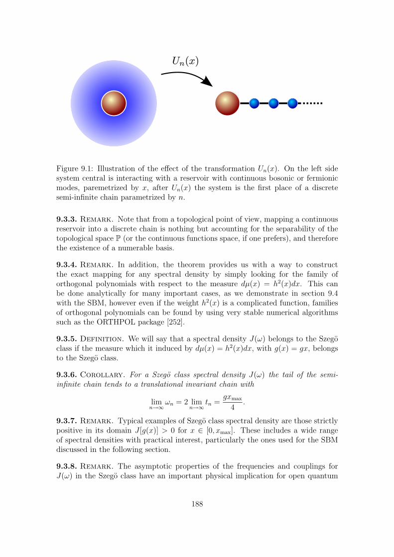
Figure 9.1: Illustration of the effect of the transformation Un(x). On the left sidesystem central is interacting with a reservoir with continuous bosonic or fermionicmodes, paremetrized by x, after Un(x) the system is the first place of a discretesemi-infinite chain parametrized by n.
9.3.3. Remark. Note that from a topological point of view, mapping a continuousreservoir into a discrete chain is nothing but accounting for the separability of thetopological space P (or the continuous functions space, if one prefers), and thereforethe existence of a numerable basis.
9.3.4. Remark. In addition, the theorem provides us with a way to constructthe exact mapping for any spectral density by simply looking for the family oforthogonal polynomials with respect to the measure dµ(x) = h2(x)dx. This canbe done analytically for many important cases, as we demonstrate in section 9.4with the SBM, however even if the weight h2(x) is a complicated function, familiesof orthogonal polynomials can be found by using very stable numerical algorithmssuch as the ORTHPOL package [252].
9.3.5. Definition. We will say that a spectral density J(ω) belongs to the Szegoclass if the measure which it induced by dµ(x) = h2(x)dx, with g(x) = gx, belongsto the Szego class.
9.3.6. Corollary. For a Szego class spectral density J(ω) the tail of the semi-infinite chain tends to a translational invariant chain with
limn→∞
ωn = 2 limn→∞
tn =gxmax
4.
9.3.7. Remark. Typical examples of Szego class spectral density are those strictlypositive in its domain J [g(x)] > 0 for x ∈ [0, xmax]. These includes a wide rangeof spectral densities with practical interest, particularly the ones used for the SBMdiscussed in the following section.
9.3.8. Remark. The asymptotic properties of the frequencies and couplings forJ(ω) in the Szego class have an important physical implication for open quantum
188
systems. Away from the quantum system, the chain becomes effectively translation-ally invariant and it is a standard exercise in condensed matter physics to diagonalizesuch a chain in terms of plane waves [253]. For chains derived from a Szego classJ(ω), the dispersion ωk of the eigenstates of the asymptotic region of the chain isωk = ωc(1 − cos(πk))/2 where the momentum runs from 0 to 1 (ωc = g(1)). Thisresult shows rigorously that the asymptotic region can support excitations over thefull spectral range of the original environment, as one would intuitively expect onphysical grounds. The translational invariance of the asymptotic region means thatexcitations of the environment can propagate away from the quantum system with-out scattering and are effectively “lost” irreversibly to the environment over time.
9.3.9. Remark. A spectral function that appears in nature, most notably in pho-tonic crystals, but which does not fall into the Szego class would be a spectralfunction that contains gaps, for instance
J(ω) = [J1(ω)θ(ω1 − ω) + J2(ω)θ(ω − ω2)]θ(ωc − ω).
Such a spectral function is zero in the region ω1 ≤ ω ≤ ω2. However, if J1,2(ω) arein the Szego class over [0, ω1] and [ω2, ωc] respectively, then the environment canbe considered as two separate chains, for which the theorems above apply for eachseparate chain.
9.4 Applications
9.4.1 Continuous spin-boson spectral densities
As a prototypical example let us consider the spin-boson Hamiltonian which de-scribes the interaction of a TLS with an environment of harmonic oscillators [15,231]
HSB = Hloc +
∫ xmax
0
dxg(x)a†xax +1
2σ3
∫ xmax
0
dxh(x)(ax + a†x), (9.19)
where ax are bosonic operators, and the local Hamiltonian of the spin is given by,
Hloc =1
2ησ1 +
1
2εσ3. (9.20)
where σ1 and σ3 are the corresponding Pauli matrices.Firstly we will consider spectral functions bounded by a hard cut-off at an energy
ωc, hence the cut-off xmax = g−1(ωc) appearing in the integrals in (9.19), which areusually parameterized as [111,112,241]
J(ω) = 2παω1−sc ωsθ(ω − ωc), (9.21)
where α is the dimensionless coupling strength of the system-bath interaction andθ(ω − ωc) denotes the Heaviside step function. In the SBM literature, spectral
189
functions with s > 1 are referred to as super-ohmic, s = 1 as Ohmic, and s < 1 assub-Ohmic. The sub-ohmic and Ohmic cases are known to show interesting criticalbehaviour at zero temperaure as a function of α [15, 231]. According to (9.14) andour convention in taking linear dispersion relations, this continuous spectral functionis related to the Hamiltonian parameters by,
g(x) = ωcx, (9.22)
h(x) =√
2αωcxs/2. (9.23)
With this choice of g(x) and h(x), xmax = 1 and absorbing the common factorωc
√2α in the system operator A = ωc
√2ασ3, the following matrix elements generate
the mapping onto the chain,
Un(x) = xs/2P (0,s)n (x), (9.24)
here P(0,s)n (x) = P
(0,s)n (x)N−1
n is a (normalized) shifted Jacobi polynomial (fromsupport [-1,1] to support [0,1]) for which the orthogonality condition reads
∫ 1
0
dxxsP (0,s)n (x)P (0,s)
m (x) = δnmN2n, (9.25)
N2n =
1
2n + s + 1. (9.26)
Therefore we get
A
∫ 1
0
dxh(x)(ax + a†x) =1
2σ3
√η0
π(b0 + b†0),
where η0 =∫ ωc
0J(ω) dω as defined by Bulla et al. [111,112,241] in their NRG study
of the SBM. They also use a mapping of the SBM onto a chain, however in theircase the mapping is performed on an approximate discretised representation of theoscillator reservoir, see section 9.4.2.
For the transformed of∫ xmax
0dxg(x)a†xax we obtain from the recursion coefficients
of the Jacobi polynomials [251], frequencies and tunneling amplitudes to be
ωn =ωc
2
(1 +
s2
(s + 2n)(2 + s + 2n)
), (9.27)
tn =ωc(1 + n)(1 + s + n)
(s + 2 + 2n)(3 + s + 2n)
√3 + s + 2n
1 + s + 2n. (9.28)
It is quite easy to check that the measure dµ(x) = xsdx belongs to the Szegoclass for any s < ∞, the integral (9.9) on [0, 1] is
∫ 1
0
ln(xs)dx√1− (2x− 1)2
= −πs ln(2).
190
Thus limn→∞ αn = 12
and limn→∞ β′n = m2
4= 1
16, so:
limn→∞
ωn =ωc
2, lim
n→∞tn =
ωc
4,
as it can be seen directly from the expressions (9.27) and (9.28). Interestingly,smaller values of s lead to faster convergence of ωn, tn towards these limits as nincreases.
If instead of a hard cut-off we use an exponential cut-off for the spectral function
J(ω) = 2παω1−sc ωse−
ωωc ,
and an integral on [0,∞), then for g(x) = ωcx we find
h(x) =√
2αωcxs/2e−s/2,
the transformation to the chain can achieved using
Un(x) = xs/2Lsn(x) = xs/2e−s/2Ls
n(x)N−1n , (9.29)
where Lsn(x) is an associated Laguerre polynomial and Nn is the normalisation of
the orthogonality relation for the associated Laguerre polynomials:
∫ 1
0
dxxse−xLsn(x)Ls
m(x) = δnmN2n, (9.30)
N2n =
Γ(n + s + 1)
n!. (9.31)
So the transformation reads
A
∫ ∞
0
dxh(x)(ax + a†x) =1
2σ3c0(b0 + b†0),
with c0 = ωc
√2αΓ(s + 1) =
√η0 where η0 =
∫∞0
J(ω) dω; and for the other termfrom the recurrence relations of the associated Laguerre polynomials [251], the fre-quencies and tunneling are
ωn = ωc (2n + 1 + s) , (9.32)
tn = ωc
√(n + 1)(n + s + 1). (9.33)
9.4.2 Discrete spectral densities. The logarithmically dis-cretized spin-boson model
Our main result (Theorem 9.3.2) maps continuous environments onto discrete semi-infinite chains which are ideal for t-DMRG simulation. However in some situationswe may want to simulate systems which are coupled to a discrete set of oscillators
191
which are not described by a continuous spectral function. This may occur physicallyin many ways, for example systems coupled to vibrations of small or finite-sizedenvironments are coupled to discrete spectral densities. Many of these discreteenvironments can be still be transformed into a chain using the same procedure wehave presented for the continuous mapping, the only different is that one now makesuse of the classical discrete orthogonal polynomials [254]. One example of this isthe finite-size discretisation of the spectral densities considered in section 9.4.1. Itwill be shown in section 9.4.3 that these discrete environments can be mapped ontochains suitable for t-DMRG analysis using the classical Hahn polynomials. In thissubsection we wish to focus on another important class of discrete spectral densitieswhich are logarithimcally discretised approximations to continuous environments.These discretised spectral densities are a key part of the powerful NRG algorithmused to study condensed matter systems, and a detailed description of this numericalmethod and the reasons for performing this discretisation are given in Refs. [111,112,241].
In the NRG approach to the same SBM considered in section 9.4, the contin-uous spin-boson Hamiltonian is approximated by representing all the modes in aenergy range ωc∆
−n − ωc∆−n−1 by a single effective degree of freedom described by
creation and annihilation operators an, a†n. These modes may either be fermionic orbosonic. The logarithmic discretisation parameter ∆ is always greater than unity,and the original continuum spin-boson Hamiltonian is recovered by sending ∆ → 1.Assuming a spectral density of the form J(ω) = 2παω1−s
c ωsθ(ωc − ω), this logarith-mic discretisation procedure generates a discrete spin-boson Hamiltonian HL of theform [111,112,241],
HL = Hloc +σz
2√
π
∞∑n=0
γn(an + a†n) +∞∑
n=0
ζna†nan, (9.34)
where
γ2n =
2πα
1 + sω2
c (1−∆−(1+s))∆−n(1+s) = γs∆−n(1+s), (9.35)
ζn =s + 1
s + 2
1−∆−(s+2)
1−∆−(s+1)ωc∆
−n = ζs∆−n. (9.36)
As described in detail in Refs. [111,112,241], the NRG algorithm can only be appliedafter the Hamiltonian HL of Eq. (9.34) is mapped onto a 1 −D nearest-neighborschain of the form,
Hc = Hloc +1
2
√η0
πσz(b0 + b†0) +
∑n
ωnb†nbn + tnb†n+1bn + tnb
†nbn+1. (9.37)
192
To do this Bulla et al. [111,112,241] first introduce a new set of bosonic modes bn, b†n
defined by an orthogonal transformation U which acts on the an, a†n,
b†n =∑m
Unma†m, (9.38)
bn =∑m
Unmam. (9.39)
They then derive the following recurrence relation for the matrix elements Unm thatbring the Hamiltonian of (9.34) to the chain form of (9.37) [111,112,241],
ζnUmn = ωmUmn + tmUm+1n + tm−1Um−1n. (9.40)
This recurrence relation is then solved numerically by an iterative procedure to pro-vide the hopping parameters tn and site energies ωn which are the input parametersfor the NRG algorithm. This recurrence relation is the standard method for findingthe chain parameters for almost all numerical simulation methods that use the chainrepresentation for impurity problems at present. However the numerical solutionsof the recurrence relations are highly sensitive to numerical noise and are often un-stable as the dimension of U becomes large. In Refs. [111,112,241] it is stated thatnumerical instabilities typically appear after about 25 − 30 iterations. The resultspresented in this paper show that the problem of implementing this chain mappingeffectively amount to the problem of finding a suitable basis of orthogonal poly-nomials to represent the bath degrees of freedom. The recursive method given byBulla et al. [111, 112, 241] is in fact equivalent to the recursive Stieltjes method fordetermining the coefficients of orthogonal polynomials, a procedure which is well-known to be numerically unstable for many weight functions, and in certain cases isso inaccurate that it completely fails for all practical purposes [255]. As orthogonalpolynomials are very useful and widely used in numerical quadrature, the problemof determining recurrence coefficients accurately for arbitrary weight functions hasbeen investigated in detail, and alternative numerical algorithms for determiningrecurrence coefficients to arbitrary accuracy have been developed, most notably theORTHPOL package of Gautschi [252]. Our results showing that the chain mappingcan always be cast as a problem of finding recurrence coefficients of orthogonal poly-nomials has thus allowed us to make use of these methods, therefore removing theissue of numerical stability from the general problem.
However, for the specific example considered in this section we can in fact solvethe recursion relation analytically, and can give explicit formulae for the parameterstn, ωn. We now demonstrate that the solution Unm to the recurrence relation of[111,112,241] can be written as,
Unm =∆−m(1+s)
2 pn(∆−m, ∆−s, 1|∆−1)
Nn
, (9.41)
where the functions pn(∆−m, ∆−s, 1|∆−1) in Eq. (9.41) are known as the little-q Jacobi polynomials [256]. These polynomials obey the following orthogonality
193
relation which defines the normalization constants Nn that appear in Eq. (9.41),
δnmN2n =
∞∑
k=0
∆−k(1+s)pn(∆−k, ∆−s, 1|∆−1)pm(∆−k, ∆−s, 1|∆−1), (9.42)
N2n =
∆−n(1+s)(∆−1; ∆−1)2n
(∆−(s+1); ∆−1)2n(1−∆−(2n+1+s))
. (9.43)
In Eq. (9.43) (a : q)n is the q-shifted factorial described in [256], and defined as
(a : q)n = (1− a)(1− aq)(1− aq2)...(1− aqn−1). (9.44)
Noting that p0(x, a, b|q) = 1 [256],
∞∑
k=0
∆−k(1+s)pn(∆−k, ∆−s, 1|∆−1) = δ0nN20 , (9.45)
= δ0n1
1−∆−(s+1). (9.46)
One further property of the little-q Jacobi polynomials that we require to performthe chain mapping is their three-term recurrence relation. This is given by,
∆−npj(∆−n, ∆−s, 1|∆−1) = (Aj + Cj)pj(∆
−n, ∆−s, 1|∆−1)
− Ajpj+1(∆−n, ∆−s, 1|∆−1)
− Cjpj−1(∆−n, ∆−s, 1|∆−1), (9.47)
where,
Aj = ∆−j (1−∆−(j+1+s))2
(1−∆−(2j+1+s))(1−∆−(2j+2+s)), (9.48)
Cj = ∆−(j+s) (1−∆−j)2
(1−∆−(2j+s))(1−∆−(2j+1+s)). (9.49)
Using the orthogonality relations one can easily show that the transformation Uis an orthogonal matrix and that the bn, b†n operators obey the same bosonic orfermionic commutation relations as the an, a
†n operators.
Now we express the original Hamiltonian in terms of the bn, b†n operators. The
second term of (9.34) transforms as,
∞∑n=0
γn(an + a†n) =∞∑
n=0
∞∑
k=0
γnUkn(bk + b†k)
= γs
∞∑
k=0
N−1k (bk + b†k)
∞∑n=0
∆−n(1+s)pk(∆−n, ∆−s, 1|∆−1)
= γs
∞∑
k=0
N−1k (bk + b†k)δ0kN
2k
= γsN0(b0 + b†0) =√
η(b0 + b†0),
194
where we have used property of Eq. (9.46) and in the last step the explicit form ofγsN0 has been used,
γ2sN
20 =
2πα
1 + sω2
c =
∫ ωc
0
J(ω)dω = η0.
where η0 is the coupling defined by Bulla et al. [111, 112, 241]. The chain couplingsand energies arise from the transformation of the third term of (9.34), which thenbecomes,
∞∑n=0
ζna†nan =
∞∑n=0
∞∑
j,k=0
ζs∆−nb†jbkUjnUkn
= ζs
∞∑
j,k=0
b†jbk
NjNk
×∞∑
n=0
∆−n(1+s)︷ ︸︸ ︷∆−npj(∆
−n, ∆−s, 1|∆−1) pk(∆−n, ∆−s, 1|∆−1).
The orthogonality condition cannot be used directly here as the weight function ofthe sum ∆−n(s+1) is multiplied by an extra factor of ∆−n. However, we can absorbthis factor in the sum using the recurrence relation of the little-q polynomials onthe braced term above. Substituting the right hand side of the recurrence relationinto Eq. (9.50) allows the orthogonality relations to be used, and ensures thatthe resulting couplings are nearest-neighbors only. This generates a 1 − D chainHamiltonian H ′ of the form of (9.16), with energies ωn and hopping tn given by,
ωn = ζs(An + Cn), (9.50)
tn = −ζs
(Nn+1
Nn
.
)An (9.51)
We now show that our explicit form for Umn in terms of little-q Jacobi polyno-mials satisfies the recurrence equation of Bulla et al. Eq. (9.40). We first use Eqs.(9.50) and (9.51) to express the right hand side of (9.40) in terms of the little-qJacobi recurrence coefficients An, Cn. Substituting ζn = ζs∆
−n on the left hand sideas well, one obtains
ζs∆−nUmn = ζs(Am + Cm)Umn − ζs
(Nm+1
Nm
)AmUm+1n (9.52)
− ζs
(Nm
Nm−1
)Am−1Um−1n. (9.53)
Now substitute for the Umn using (9.41) we obtain,
∆−npm(∆−n, ∆−s, 1|∆−1) = (Am + Cm)pm(∆−n, ∆−s, 1|∆−1)
+
(Nm
Nm−1
)2
Am−1pm−1(∆−n, ∆−s, 1|∆−1)
+ Ampm+1(∆−n, ∆−s, 1|∆−1).
195
The final additional that result we need to use is that the following relationsholds,
Cm = Am−1
(Nm
Nm−1
)2
m > 1, (9.54)
C0 = 0 m = 0, (9.55)
which is easily shown from the definitions of Am, Cm. Substituting this into Eq.(9.56),the equation reduces to,
∆−npm(∆−n, ∆−s, 1|∆−1) = (Am + Cm)pm(∆−n, ∆−s, 1|∆−1)
+ Ampm+1(∆−n, ∆−s, 1|∆−1)
+ Cmpm−1(∆−n, ∆−s, 1|∆−1).
This is just the recurrence relation for the little-q Jacobi polynomials. Thereforethe original Unm of Eq. (9.41) is the solution of the recurrence relations of Bulla etal.. The energies and hopping amplitudes are simple functions of An, Cn and thefollowing additional relation can also be derived using Eqs. (9.50) and (9.51),
ωn = −tn
(Nn
Nn+1
)− tn−1
(Nn−1
Nn
).
9.4.3 Linearly-discretised baths
We now consider an environment consisting in a large, but discrete number N + 1of environmental degrees of freedom. The Hamiltonian for such a system can bewritten as
H = Hloc +σz
2√
π
N∑n=0
γn(an + a†n) +N∑
n=0
ζna†nan, (9.56)
where ζn = ωcn/(N + 1), the coupling constants γn are
γ2n = 2πα
ω2c
(N + 1)s+1
(s + n
n
), (9.57)
and the bosonic operators obey the discrete commutation relation [an, a†m] = δnm.
The expressions for ζn and γn arise from a linear discretisation of the continuousspectral function J(ω) = 2παω1−s
c ωs with N + 1 oscillators equally-spaced in kapproximating the bath. As N → ∞ we recover the continuum limit which wasmapped using Jacobi polynomials. This discrete Hamiltonian can be mapped to thenearest-neighbors chain using the orthogonal transformation
bk =N∑
n=0
(s + n
n
) 12
Qk(n, s)ρ−1k an, (9.58)
196
where Ql(n, s) = Ql(n, s, 0, N) is a Hahn polynomial [254, 256]. The Hahn polyno-mials are classical discrete orthogonal polynomials and are defined by the discreteinner product
N∑n=0
(α + n
n
)(β + N − x
N − x
)Ql(n, α, β,N)Qk(n, α, β,N) = ρ2
kδlk. (9.59)
Introducing the Pochhammer symbol (a)k = a(a+1)...(a+N−1), the normalizationfactors ρk are given by
ρk =(−1)k(k + α + β + 1)N+1(β + 1)kk!
(2k + α + β + 1)(α + 1)k(−N)kN !. (9.60)
Using the inner product relation is it easy to show that the new modes bk, b†k obey
the same commutation relations as the original modes, and using the identity [256],
(s + x
x
)(s + y
y
) N∑
k=0
Qk(x, α, β,N)Qk(y, α, β, N)
ρ2k
= δxy, (9.61)
one can show that the inverse transform is
an =N∑
k=0
(s + n
n
) 12
Qk(n, s)bk. (9.62)
The Hahn polynomials also obey the three-term recurrence relation
xQn(x, α, β, N) = AnQn+1(x, α, β, N)− (An + Cn)Qn(x, α, β, N)
+ CnQn−1(x, α, β, N), (9.63)
where
An =(n + α + β + 1)(n + α + 1)(N − n)
(2n + α + β)(2n + α + β + 1), (9.64)
Cn =n(n + α + β + N + 1)(n + β)
(2n + α + β)(2n + α + β + 1). (9.65)
We now substitute (9.62) into H to obtain the chain Hamiltonian. As in the previ-ous examples, the three-term recurrence and orthogonality of the Qk(n, s) ensuresthe generation of a discrete nearest-neighbors chain with energies and couplings de-termined by the recurrence coefficients of the Hahn polynomials. The transformedHamiltonian Hc is given by,
Hc = Hloc +1
2
√η
πσz(b0 + b†0) +
N∑n=0
ωnb†n + tnb†nbn+1 + tnb†n+1bn, (9.66)
ωn =ωc
N + 1(An + Cn), (9.67)
tn =ωc
N + 1
ρn+1
ρn
An. (9.68)
197
The discrete weight function is not in the Szego class, and at finite N we findthat ωn → ωc/4, tn → 0 as n → N . However, taking the limit N → ∞ leads tothe recovery of the results obtained for a continuous power-law spectral density insection 9.4.1. Formally this results from the limit relation [256],
limN→∞
Qn(Nx, a, b, N) = (−1)nP a,bn (2x− 1)/P a,b
n (1),
although this can also be seen by using taking the limit of the explicit expressionsfor the recurrence relations An, Cn and normalizations Nn for the Hahn polynomials.Using the explicit expressions, it is also easy to show that the difference betweenthe chain energies and hoppings for the continuous and linearly discretized bath areof O(n/N) for n ¿ N . The differences in the behaviour of the chain parameters inthe finite and continuous cases has a physical significance that will be explored ina future work. Here, it will be enough to say the vanishing of the tn as n → ∞ isrelated to the existence of a recurrence time in the dynamics of the discrete problem.
9.5 Conclusions
In this chapter we have demonstrated how the problem of a quantum system coupledlinearly to the coordinates of a continuous bosonic or fermionic environment can bemapped exactly onto a one-dimensional model with only short-range interactions.Using the theory of orthogonal polynomials, we have shown how the parametersof this one dimensional representation can be simply obtained from the recurrencecoefficients of the orthogonal polynomials of the spectral function describing the en-vironment. Certain important spectral functions correspond to the weight functionsof the classical orthogonal polynomials, and the parameters of the chain Hamilto-nian can be given in closed analytical form. When the spectral function is not aclassical weight function, we can make use of numerical techniques developed for de-termining recurrence coefficients that allow us to find the chain parameters to highprecision and for arbitrary long chains. Our use of orthogonal polynomials simul-taneously removes the need to discretise the environmental degrees of freedom andalso the numerical instabilities that plague the recursive method previously used toimplement this chain transformation. This is particularly important, as hitherto theprincipal use of the chain transformation is to enable numerical simulation of thedynamics and ground state properties of systems which strongly interact with theirenvironments. The work presented here was principally motivated by an attempt touse the powerful t-DMRG simulation technique to study strongly-interacting openquantum systems, a problem of considerable topically, especially in the emergingfield of quantum effects in biology. The combination of our exact mapping has nowmade it possible to use t-DMRG to obtain extremely accurate simulations of open-system dynamics with no artefacts arising from having a discretised representationof the environment and a numerical approximation to the mapping. Using the the-ory of orthogonal polynomials, we have also given examples that could be used inthe NRG community.
198
In addition to these practical advantages, the analytical mapping reveals an in-teresting structure to the system-environment systems we consider, in particular,the result that the chain representations of all spectral functions in the physicallybroad, Szego class look the same in the asymptotic limit. This observation may leadto further improvements in the numerical efficiency of open-quantum simulations,allowing the chain representations to be truncated in an efficient way that is uni-versal for all spectral functions in the Szego class. We have also presented resultsshowing the relations between the chain representations of linearly and logarith-mically discretised spin-boson models and the continuous case, results which mayalso prove useful in determining how to optimize the accuracy of simulations witha discretised representations.
199

Prospects
The topics that have been presented in this thesis have prompted new questionswhich could be the potential focus of subsequent work.
Starting with Markovian dynamics, there are many open questions to answer forinteracting systems, mainly in non-equilibrium situations arising from weak couplingto baths with different temperatures. For instance, what is the connection betweenthe strength of the system interaction and the energy flux from the hotter to thecooler bath? Once this connection is established, we can ask what is the best strategyto obtain a Markovian master equation describing such a flux of energy.
Additionally, we have given an example of entangled steady states assisted byMarkovian noise (chapter 6). The preparation of entangled states via dissipationis an active field of research, see for example [257–262] for recent developments.Actually, the first experiment which implements this idea has already been carriedout [263]. However, there is not a general classification of the type of completelypositive semigroups with entangled asymptotic states.
The microscopic structure of the environment in solid-state qubits is still notfully characterized. As analyzed in chapter 8, it seems that the most realistic modelrequire the introduction of an ensemble of two-level fluctuators. However, the truenumber of fluctuators which are involved in the decoherence process is not clear, noris it known if these fluctuators interact with each other. In fact this later point hasnot been explored in real experiments, so the method we propose could be a firststep towards analyzing this.
Regarding non-Markovian dynamics there is still a plethora of open problems.It is of particular importance to design new methods to describe them when the ex-isting non-Markovian techniques are not applicable. In this context, we introducedin chapter 9 an exact method to map a reservoir into a chain with nearest-neighborsinteractions which allows us to outperform previous methods of numerical simula-tion. We stress here that, for a wide class of spectral densities, it is possible toconsider the asymptotic region of the chain as a secondary environment, in whichcase the system–bath Hamiltonian can be recast as a finite chain in which the finalmode is damped by the translationally invariant chain. In this picture, the dampingof the final member of the chain is universal for all spectral densities in the Szego
201
class. Such a truncated picture might allow for improved efficiency in the numericalsimulation of open-system dynamics, and the detailed physics behind this intuitivelyappealing picture of relaxation and dephasing in the chain picture is currently underinvestigation and will be published elsewhere.
Work presented in chapter 7 is receiving increasing attention, and is regarded aspioneering in the field. Nowadays, this is a very active area of research and a surgeof new papers have recently been published [264–272]. There are many interestingquestions to pose about this topic, including establishing possible relations betweennon-Markovianity and other characteristics of an open quantum system. For exam-ple, the efficiency in the transport of excitations, the stability of the motion or itschaotic properties, as well as the preservation of quantum properties in time. In thissense, we have found some examples where the presence of non-Markovianity canbe quantitatively linked to the existence of entangled asymptotic states.
On the other hand, it is not clear whether Markovianity in the classical sensecorresponds to Markovianity in the quantum sense given a dynamical map as asuccessive application of random unitary transformations. For this, the randomnessis given by a classical random variable. Actually, preliminary results suggest thatthis is not the case [273,274].
Finally, we are carrying out studies about some other topics related to opensystem dynamics. Particularly, we are investigating under which circumstances anenvironment can be consider as “classical”, such that the dynamics are just a convexcombination of unitary maps. For a qubit, this is the case for any dynamics whichpreserve the identity (unital), see [33, 275]. However we have developed models forthe description of possible noise-assisted biological processes where this is not thecase [276]. Even so, that an environment can be classically reproducible does notseem to be essential for the efficiency of those processes, as least within our currentunderstanding of the energy transfer dynamics.
202
Bibliography
[1] M. Planck. Annalen der Physik 4, 553 (1901).
[2] W. H. Louisell, Quantum Statistical Properties of Radiation, John Wiley &Sons Inc, New York, 1973.
[3] E. B. Davies, Quantum Theory of Open Systems, Academic Press, London,1976.
[4] C. Cohen-Tannoudji, J. Dupont-Roc and G. Grynberg, Atom-Photon Interac-tions, John Wiley & Sons, New York, 1992.
[5] H. Carmichael, An Open Systems Approach to Quantum Optics, Springer,Berlin, 1993.
[6] K. Blum, Density Matrix Theory and Applications, Plenum Press, New York,1996.
[7] R. Zwanzig, Nonequilibrium Statistical Mechanics, Oxford University Press,New York, 2001.
[8] R. Alicki and M. Fannes, Quantum Dynamical Systems, Oxford UniversityPress, New York, 2001.
[9] G. Lindblad, Non-Equilibrium Entropy and Irreversibility, Reidel PublishingCompany, Dordrecht, 2001.
[10] B. Fain, Irreversibilities in Quantum Mechanics, Kluwer Academic Publishers,New York, 2002.
[11] H. -P. Breuer and F. Petruccione, The Theory of Open Quantum Systems,Oxford University Press, Oxford, 2002.
[12] E. Joos, H. D. Zeh, C. Kiefer, D. J. W. Giulini, J. Kupsch, I. -O. Stamatescu,Decoherence and the Appearance of a Classical World in Quantum Theory,Springer, Berlin, 2003.
203
[13] C. W. Gardiner and P. Zoller, Quantum Noise, Springer, Berlin, 2004.
[14] S. Attal, A. Joye and C. -A. Pillet (eds.), Open Quantum Systems (3 vols.),Springer, Berlin, 2006.
[15] U. Weiss, Quantum Dissipative Systems, World Scientific, Singapore, 2008.
[16] E. Kreyszig, Introductory Functional Analysis with Applications, Wiley, NewYork, 1978.
[17] M. Reed and B. Simon, Methods of Modern Mathematical Physics I, AcademicPress, San Diego, 1980.
[18] N. Bocccara, Functional Analysis: An Introduction for Physicists, AcademicPress, 1990.
[19] A. Galindo and P. Pascual, Problemas de Mecanica Cuantica, Eudema,Madrid, 1989.
[20] M. Spivak, Calculus, Cambridge University Press, Cambridge, 1994.
[21] K. Yosida, Functional Analysis, Springer, Berlin, 1980.
[22] M. Reed and B. Simon, Methods of Modern Mathematical Physics II, AcademicPress, San Diego, 1975.
[23] K. -J. Engel and R. Nagel, One-Parameter Semigroups for Linear EvolutionEquations, Springer, New-York, 2000.
[24] The most simple example is in one dimension, take a nowhere differentiablefunction f(t) and define T(t,s) = f(t)/f(s) for f(s) 6= 0.
[25] F. Schwabl, Quantum Mechanics, Springer, Berlin, 2007.
[26] E. Schrodinger, Phys. Rev. 28, 1049 (1926).
[27] One point to stress here is that a quantum system that interchanges informa-tion with a classical one in a controllable way (such as a pulse of a laser fieldinteracting an atom) is also considered isolated.
[28] R. Gahler, A. G. Klein and A. Zeilinger, Phys. Rev. A 23, 1611 (1981).
[29] S. Weinberg, Phys. Rev. Lett. 62, 485 (1989).
[30] J. J. Bollinger, D. J. Heinzen, Wayne M. Itano, S. L. Gilbert and D. J.Wineland, Phys. Rev. Lett. 63, 1031 (1989).
[31] A. Galindo and P. Pascual, Quantum Mechanics (2 vols), Springer, Berlin,1990.
204
[32] It can be shown that it is the only linear (isomorphic) isometry of trace-classoperators. Actually the proof of theorem 3.2.5 is similar.
[33] M. A. Nielsen and I. L. Chuang, Quantum Computation and Quantum Infor-mation, Cambridge University Press, Cambridge, 2000.
[34] S. Virmani, Entanglement Quantification & Local Discrimination, PhD Thesis,Imperial College London, 2001.
[35] P. Stelmachovic and V. Buzek, Phys. Rev. A 64, 062106 (2001).
[36] Leaving aside the case of factorized global dynamics U(t1, t0) = UA(t1, t0) ⊗UB(t1, t0), see: D. Salgado and J. L. Sanchez-Gomez, Comment on “Dynamicsof open quantum systems initially entangled with environment: Beyond theKraus representation” quant-ph/0611222 (2003); H. Hayashi, G. Kimura andY. Ota, Phs. Rev. A 67, 062109 (2003).
[37] A. Peres, Quantum Theory: Concepts and Methods, Kluwer Academic Pub-lishers, Dordrecht, 1995.
[38] L. E. Ballentine, Quantum Mechanics: A Modern Development, World Scien-tific, Singapore, 1998.
[39] T. F. Jordan, A. Shaji and E. C. G. Sudarshan, Phys. Rev. A 70, 052110(2004).
[40] A. Shaji and E. C. G. Sudarshan, Phys. Lett. A 341, 48 (2005).
[41] A. Shaji, Dynamics of initially entangled open quantum systems, PhD Thesis,University of Texas at Austin, 2005.
[42] H. A. Carteret, D. R. Terno and K. Zyczkowski, Phys. Rev. A 77, 042113(2008).
[43] D. Salgado, J. L. Sanchez-Gomez and M. Ferrero, Phys. Rev. A 70, 054102(2004).
[44] D. M. Tong, L. C. Kwek, C. H. Oh, J. -L. Chen and L. Ma, Phys. Rev. A 69,054102 (2004).
[45] P. Pechukas, Phys. Rev. Lett. 73, 1060 (1994).
[46] A. J. van Wonderen and K. Lendi, J. Phys. A: Math. Gen. 33, 5557 (2000).
[47] C. A. Rodrıguez, K. Modi, A. Kuah, A. Shaji and E. C. G. Sudarshan, J.Phys. A: Math. Gen. 41, 205301 (2008).
[48] A. Shabani and D. A. Lidar, Phys. Rev. Lett. 102, 100402 (2009).
[49] W. Stinespring, Proc. Am. Math. Soc. 6, 211 (1955).
205
[50] K. Kraus, States, Effects, and Operations Fundamental Notions of QuantumTheory, Lect. Notes Phys. 190, Springer, Berlin, 1983.
[51] A. Kossakowski, Rep. Math. Phys. 3, 247 (1972).
[52] A. Kossakowski, Bull. Acad. Polon. Sci. Math. 20, 1021 (1972).
[53] M. B. Ruskai, Rev. Math. Phys. 6, 1147 (1994).
[54] Note that the composition of two completely positive maps is also a com-pletely positive map. However the composition of two arbitrary maps canbe completely positive regardless of whether they are individually completelypositive or not.
[55] C. A. Rodriguez-Rosario and E. C. G. Sudarshan, Non-Markovian Open Quan-tum Systems quant-ph/08031183 (2008).
[56] C. W. Gardiner, Handbook of Stochastic Methods, Springer, Berlin, 1997.
[57] J. R. Norris, Markov Chains, Cambridge University Press, Cambridge, 1997.
[58] S. N. Ethier and T. G. Kurtz, Markov Processes: Characterization and Con-vergence, Wiley, New Jersey, 2005.
[59] R. Alicki and K. Lendi, Quantum Dynamical Semigroups and Applications,Lect. Notes Phys. 286, Springer, Berlin, 1987.
[60] Another proof of sufficiency can be found in Appendix E of [133].
[61] V. Gorini, A. Kossakowski and E. C. G. Sudarshan, J. Math. Phys. 17, 821(1976).
[62] G. Lindblad, Commun. Math. Phys. 48, 119 (1976).
[63] F. Benatti and R. Floreanini, Int. J. Mod. Phys. B 19, 3063 (2005).
[64] F. Benatti, A. M. Liguori and A. Nagy, J. Math. Phys. 49, 042103 (2008).
[65] R. A. Horn and C. R. Johnson, Topics in Matrix Analysis, Cambridge Uni-versity Press, Cambridge, 1991.
[66] D. Burgarth and V. Giovannetti, New J. Phys. 9, 150 (2007).
[67] H. Spohn, Rev. Mod. Phys. 53, 569 (1980).
[68] E. B. Davies, Commun. Math. Phys. 19, 83 (1970).
[69] H. Spohn, Rep. Math. Phys. 10, 189 (1976).
[70] H. Spohn, Lett. Math. Phys. 2, 33 (1977).
206
[71] D. E. Evans, Commun. Math. Phys. 54, 293 (1977).
[72] A. Frigerio, Lett. Math. Phys. 2, 79 (1977).
[73] A. Frigerio, Commun. Math. Phys. 63, 269 (1978).
[74] A. Frigerio and H. Spohn, Stationary states of quantum dynamical semigroupsand applications, in: L. Accardi, V. Gorini, G. Paravicini, (eds.), Proceedingsof Mathematical Problems in the Theory of Quantum Irreversible Processes,pp. 115-135, Laboratoria di Cibernetica del CNR, 1978.
[75] B. Baumgartner, H. Narnhofer and W. Thirring, J. Phys. A: Math. Theor.41, 065201 (2008).
[76] B. Baumgartner and H. Narnhofer, J. Phys. A: Math. Theor. 41, 395303(2008).
[77] L. Jansen and H. Boon, Theory of Finite Groups. Application in Physics,North-Holland, Amsterdam, 1967.
[78] S. Nakajima, Progr. Theor. Phys. 20, 984 (1958).
[79] R. Zwanzig, J. Chem. Phys. 33, 1338 (1960).
[80] F. Haake Statistical Treatment of Open Systems by Generalized Master Equa-tions (Springer Tracts in Modern Physics) vol 66, Springer, Berlin, pp 98-168.
[81] R. R. Puri, Mathematical Methods of Quantum Optics, Springer, Berlin, 2001.
[82] C. Chicone, Ordinary Differential Equations with Applications, Springer, NewYork, 2006.
[83] E. L. Ince, Ordinary Differential Equations, Dover, New York, 1956.
[84] S. Kryszewski and J. Czechowska-Kryszk, Master equation - tutorial approachquant-ph/08011757 (2008).
[85] R. S. Whitney, J. Phys. A: Math. Theor. 41, 175304 (2008).
[86] E. B. Davies, Commun. Math. Phys. 39, 91 (1974).
[87] E. B. Davies, Math. Ann. 219, 147 (1976).
[88] V. Gorini and A. Kossakowski, J. Math. Phys. 17, 1298 (1976).
[89] A. Frigerio and V. Gorini, J. Math. Phys. 17, 2123 (1976).
[90] A. Frigerio, C. Novellone and M. Verri, Rep. Math. Phys. 12, 279 (1977).
[91] M. Ziman, P. Stelmachovic and V. Buzek, Open Syst. Inf. Dyn. 12, 81 (2005).
207
[92] M. Ziman and V. Buzek, Phys. Rev. A 72, 022110 (2005).
[93] D. Taj and F. Rossi, Phys. Rev. A 78, 052113 (2008).
[94] L. Schwartz, Theorie des Distributions, Hermann, Paris, 1973.
[95] V. S. Vladimirov, Methods of the Theory of Generalized Functions, Taylor &Francis, London, 2002.
[96] G. B. Arfken and H. J. Weber, Mathematical Methods for Physicists, AcademicPress, San Diego, 1985.
[97] R. Dumcke and H. Spohn, Z. Phys. B34, 419 (1979).
[98] Y. Zhao and G. H. Chen, Phys. Rev. E 65, 056120 (2002).
[99] A. Suarez, R. Silbey and I. Oppenheim, J. Chem. Phys 97, 5101 (1992).
[100] P. Gaspard and M. Nagaoka, J. Chem. Phys. 111, 5668 (1999).
[101] F. Benatti, R. Floreanini and M. Piani, Phys. Rev. A 67, 042110 (2003).
[102] F. Benatti, R. Floreanini and S. Breteaux, Laser Physics 16, 1395 (2006).
[103] R. Kubo, J. Phys. Soc. Jpn. 12, 570 (1957); P. C. Martin and J. Schwinger,Phys. Rev. 115, 1342 (1959).
[104] C. M. Caves and G. J. Milburn, Phys. Rev. A 36, 5543 (1987).
[105] E. B. Davies and H. Spohn, J. Stat. Phys. 19, 511 (1978).
[106] R. Alicki, J. Phys. A: Math. Gen. 12, L103 (1979).
[107] H. -P. Breuer and F. Petruccione, Phys. Rev. A 55, 3101 (1997).
[108] S. Kohler, T. Dittrich and P. Hanggi, Phys. Rev. E 55, 300 (1999).
[109] V. V. Dobrovitski and H. A. De Raedt, Phys. Rev. E 67, 056702 (2003).
[110] E. Paladino, M. Sassetti, G. Falci, U. Weiss, Phys. Rev. B 77, 041303(R)(2008).
[111] R. Bulla, H. -J. Lee, N. -H. Tong and M. Vojta, Phys. Rev. B 71, 045122(2005).
[112] R. Bulla, T. Costi and T. Pruschke, Rev. Mod. Phys. 80, 395 (2008).
[113] J. Prior, A. W. Chin, S. F. Huelga and M. B. Plenio, Phys. Rev. Lett. 105,050404 (2010).
[114] B. Vacchini and H. -P. Breuer, Phys. Rev. A 81, 042103 (2010).
208
[115] S. M. Barnett and S. Stenholm, Phys. Rev. A 64, 033808 (2001).
[116] S. Daffer, K. Wodkiewicz, J. D. Cresser and J. K. McIver, Phys. Rev. A 70,010304 (2004).
[117] H. -P. Breuer and B. Vacchini, Phys. Rev. Lett. 101, 140402 (2008).
[118] A. Shabani and D. A. Lidar, Phys. Rev. A 71, 020101(R) (2005).
[119] S. Maniscalco and F. Petruccione, Phys. Rev. A 73, 012111 (2006).
[120] S. Maniscalco, Phys. Rev. A 75, 062103 (2007).
[121] X. L. Huang and X. X. Yi, EPL 82, 50001 (2008).
[122] A. Kossakowski and R. Rebolledo, Open Syst. Inf. Dyn. 16, 259 (2009).
[123] L. Mazzola, E. -M. Laine, H. -P. Breuer, S. Maniscalco and J. Piilo, Phys.Rev. A 81, 062120 (2010).
[124] B. L. Hu, J. P. Paz and Y. Zhang, Phys. Rev. D 45, 2843 (1992).
[125] R. Karrlein and H. Grabert, Phys. Rev. E 55, 153 (1997).
[126] B. M. Garraway, Phys. Rev. A 55, 2290 (1997).
[127] H. -P. Breuer, B. Kappler and F. Petruccione, Phys. Rev. A 59, 1633 (1999).
[128] F. Shibata, Y. Takahashi and N. Hashitsume, J. Stat. Phys. 17, 171 (1977).
[129] D. Chruscinski and A. Kossakowski, Phys. Rev. Lett. 104, 070406 (2010).
[130] M. J. W. Hall, J. Phys. A: Math. Theor. 41, 269801 (2008).
[131] D. Chruscinski, A. Kossakowski, P. Aniello, G. Marmo and F. Ventriglia, Aclass of commutative dynamics of open quantum systems quant-ph/10041388(2010).
[132] D. Chruscinski and A. Kossakowski, General form of quantum evolution quant-ph/10062764 (2010).
[133] G. Schaller and T. Brandes, Phys. Rev. A 78, 022106 (2008).
[134] G. Schaller and T. Brandes, Phys. Rev. A 79, 032110 (2009).
[135] F. Benatti, R. Floreanini, U. Marzolino, EPL 88, 20011 (2009).
[136] F. Benatti, R. Floreanini, U. Marzolino, Phys. Rev. A 81, 012105 (2010).
[137] J. Eisert and M. B. Plenio, Int. J. Quant. Inf. 1, 479 (2003).
[138] D. Bures, Trans. Am. Math. Soc. 135, 199 (1969).
209
[139] H. Scutaru, J. Phys. A: Math. Gen. 31, 3659 (1998); Gh. -S. Paraoanu andH. Scutaru, Phys. Rev. A 61, 022306 (2000).
[140] In fact, note that the rotating wave Hamiltonian is not always an approx-imation, and there are physical systems which described physically by thatHamiltonian, for instance typically in situations where the total number ofexcitations is preserved.
[141] H. J. Carmichael, Statistical Methods in Quantum Optics I: Master Equationsand Fokker-Plack Equations, Springer, Berlin, 1999.
[142] M. G. A. Paris, F. Illuminati, A. Serafini and S. De Siena, Phys. Rev A 68,012314 (2003).
[143] For more details see T. Apostol, Introduction to Analytic Number Theory,Springer, New York, 1976.
[144] R. R. Puri and S. V. Lawande, Phys. Lett. 64A, 143 (1977); Phys. Lett. 69A161 (1978); R. Karrlein and H. Grabert, Phys. Rev. E 55, 153 (1997).
[145] H. Jeong, J. Lee and S. M. Kim, Phys. Rev. A 61, 052101 (2000); J. Lee, M.S. Kim and H. Jeong, Phys. Rev. A 62, 032305 (2000); S. M. Kim and J. Lee,Phys. Rev. A 66, 030301(R) (2002); S. Scheel and D. -G. Welsch, Phys. Rev.A 64, 063811 (2001); T. Hiroshima, Phys. Rev. A 63, 022305 (2001); J. S.Prauzner-Bechcicki, J. Phys. A: Math. Gen. 37, L173 (2004); J. -H. An andW. -M. Zhang, Phys. Rev. A 76, 042127 (2007); J. P. Paz and A. Roncaglia,Phys. Rev. Lett. 100, 220401 (2009); J. P. Paz and A. Roncaglia, Phys. Rev.A 79, 032102 (2009).
[146] C. -H. Chou, T. Yu and B. -L. Hu, Phys. Rev. E 77, 011112 (2008).
[147] L. E. Estes, T. H. Keil and L. M. Narducci, Phys. Rev. 175, 286 (1968).
[148] H. J. Carmichael and D. F. Walls, J. Phys. A: Math. Nucl. Gen. 6, 1552(1973).
[149] M. A. de Ponte, M. C. de Oliveira and M. H. Y. Moussa, Phys. Rev. A 70,022324 (2004); Phys. Rev. A 70, 022325 (2004); Ann. Phys. 317, 72 (2005).
[150] A. Garg, Phys. Rev. Lett., 77, 964 (1996).
[151] D. Porras, F. Marquardt, J. von Delft and J. I. Cirac, Phys. Rev. A 78,010101(R) (2008).
[152] A. Romito, R. Fazio and C. Bruder, Phys. Rev. B 71, 100501 (2005).
[153] T. Gaebel et al., Nature Phys. 2, 408 (2006).
210
[154] M. Mohseni, P. Rebentrost, S. Lloyd and A. Aspuru-Guzik, J. Chem. Phys.129, 174106 (2008).
[155] M. B. Plenio and S. F. Huelga, New J. Phys. 10, 113019 (2008).
[156] A. Olaya-Castro, C. F. Lee, F. F. Olsen and N. F. Johnson, Phys. Rev. B 78,085115 (2008).
[157] P. Rebentrost, M. Mohseni, I. Kassal, S. Lloyd and A. Aspuru-Guzik, New J.Phys. 11, 033003 (2009).
[158] F. Caruso, A. W. Chin, A. Datta, S. F. Huelga and M. B. Plenio, J. Chem.Phys. 131, 105106 (2009).
[159] M. Thorwart et al., Chem. Phys. Lett. 478, 234 (2009).
[160] R. Alicki, M. Fannes and M. Horodecki, J. Phys. A: Math. Theor. 42, 065303(2009).
[161] H. Bombin, R. W. Chhajlany, M. Horodecki and M. A. Martin-Delgado, Self-Correcting Quantum Computers quant-ph/09075228 (2009).
[162] S. Chesi, B. Rothlisberger and D. Loss, Phys. Rev. A 82, 022305 (2010).
[163] R. Benzi, A. Sutera, and A. Vulpiani, J. Phys. A 14, L453 (1981).
[164] L. Gammaitoni, P. Hanggi, P. Jung , and F. Marchesoni, Rev. Mod. Phys. 70,223 (1998).
[165] See T. Wellens, V. Shatokhin, and A. Buchleitner, Rep. Prog. Phys. 67, 45(2004).
[166] R. Lofstedt and S. N. Coppersmith, Phys. Rev. Lett. 72, 1947 (1994).
[167] M. Grifoni and P. Hanggi, Phys. Rev. Lett. 76, 161 (1996).
[168] M. Grifoni and P. Hanggi, Phys. Rev. E. 54, 1390 (1996).
[169] M. Grifoni and P. Hanggi, Phys. Rev. E. 59, 5137 (1999).
[170] A. Buchleitner and R. Mantegna, Phys. Rev. Lett. 80, 3932 (1998).
[171] S. F. Huelga and M. B. Plenio, Phys. Rev. A 62, 052111 (2000).
[172] I. Goychuk, J. Casado-Pascual, M. Morillo, J. Lehmann, P. Hanggi, Phys.Rev. Lett. 97, 210601 (2006).
[173] D. E. Makarov and N. Makri, Phys. Rev. B 52, 2257(R) (1995);
[174] T. Wellens and A. Buchleitner, Phys. Rev. Lett. 84, 5118 (2000).
211
[175] L. Viola, E. M. Fortunato, S. Lloyd, C. H. Tseng, and D. G. Cory, Phys. Rev.Lett. 84, 5466 (2000).
[176] See I. Goychuk, P. Hanggi, Adv. Phys. 54, 525 (2006); for a recent reviewdiscussing a broad class of stochastic resonance phenomena.
[177] For results concerning SR phenomena in classical arrays see, for instance, J. F.Lindner, B. K. Meadows, W. L. Ditto, M. E. Inchiosa, A. R. Bulsara, Phys.Rev. Lett. 75, 3 (1995); see also F. Marchesoni, L. Gammaitoni, A. R. Bulsara,Phys. Rev. Lett. 76, 2609 (1996); for array-enhancement effects, J.A. Acebron,W. J. Rappel, A. R. Bulsara, Phys. Rev. E 67, 016210 (2003); for a descriptionof cooperative effects, Z. Neda, Phys. Rev. E 51, 5315 (1995); for the studyof SR in a classical Ising chain.
[178] S. F Huelga and M. B. Plenio, Phys. Rev. Lett. 98, 170601 (2007).
[179] L. Henderson, V. Vedral, J. Phys. A: Math. Gen. 34, 6899 (2001).
[180] B. Schumacher, M. D. Westmoreland, Phys. Rev. A 74, 042305 (2006).
[181] I. Goychuk and P. Hanggi, New J. Phys. 1, 14 (1999).
[182] W. K. Wootters, Phys. Rev. Lett. 80, 2245 (1998) .
[183] M. B. Plenio and S. Virmani, Quant. Inf. Comp. 7, 1 (2007).
[184] P. Rebentrost, M. Mohseni, A. Aspuru-Guzik, J. Phys. Chem. B 113, 9942(2009).
[185] See H. Lee H, Y. C Cheng and G. R. Fleming, Science 316, 1462 (2007); V. I.Prokhorenko, A. R. Holzwarth, F. R. Nowak and T. J. Aartsma, J. Phys.Chem. B 106, 9923 (2002).
[186] G. S. Engel, T. R. Calhoun, E. L. Read, T. K. Ahn, T. Mancal, Y. C. Cheng,R. E. Blankenship and G. R. Fleming, Nature 446, 782 (2007).
[187] I. P. Mercer, Y. C. El-Taha, N. Kajumba, J. P. Marangos, J. W. G. Tisch, M.Gabrielsen, R. J. Cogdell, E. Springate and E. Turcu, Phys. Rev. Lett. 102,057402 (2009).
[188] C. P. Slichter, Principles of Magnetic Resonance, Springer Series in Solid-StateSciences, Berlin, 1990.
[189] A. Peres, Phys. Rev. Lett. 77, 1413 (1996); M. Horodecki, P. Horodecki andR. Horodecki, Phys. Lett. A 223, 1 (1997).
[190] M. B. Plenio and S. F. Huelga, Phys. Rev. Lett. 88, 197901 (2002).
[191] L. Hartmann, W. Dur and H.-J. Briegel, Phys. Rev. A. 74, 052304 (2006).
212
[192] L. Hartmann, W. Dur and H.-J. Briegel, New J. Phys. 9, 230 (2007).
[193] N. Lambert, R. Aguado and T. Brandes, Phys. Rev. B 75, 045340 (2007).
[194] L. D. Contreras-Pulido and R. Aguado, Phys. Rev. B 77, 155420 (2008).
[195] A. Shnirman, Y. Makhlin, and G. Schon, Phys. Scr. T102, 147 (2002).
[196] C. Di Franco, M. Paternostro, D. I. Tsomokos and S. F. Huelga, Phys. Rev.A 77, 062337 (2008).
[197] M. M. Wolf, J. Eisert, T. S. Cubitt and J. I. Cirac, Phys. Rev. Lett. 101,150402 (2008); M. M. Wolf and J. I. Cirac, Commun. Math. Phys. 279, 147(2008).
[198] H.-P. Breuer, E.-M. Laine, J. Piilo, Phys. Rev. Lett. 103, 210401 (2009).
[199] M. Ziman and V. Buzek, Phys. Rev. A 72, 052325 (2005).
[200] A very simple example is a qubit interacting via the Hamiltonian H =|01〉〈10| + |10〉〈01| with another qubit playing the role of the environment,i.e. the time evolution will swap back and forth with the evironmental qubit.Evidently this will periodically increase and decrease the entanglement be-tween an ancillary qubit and the system.
[201] M. B. Plenio, Phys. Rev. Lett. 95, 090503 (2005).
[202] A. JamioÃlkowski, Rep. Math. Phys. 3, 275 (1972); M.-D. Choi, Lin. Alg. andAppl. 10, 285 (1975).
[203] A similar result can be obtained for spontaneous emission and by using theLorentzian spectral density for the Jaynes-Cummings model we would obtaina behaviour in total agreement with the results in Fig. 2 in [198].
[204] D. Porras and J. I. Cirac, Phys. Rev. Lett. 92, 207901 (2004).
[205] E. Collini and G. D. Scholes, Science 323, 369 (2009).
[206] M .H. Devoret, A. Wallraff and J. M. Martinis, Superconducting qubits: Ashort review cond-mat/0411174 (2004).
[207] A. J. Leggett, J. Phys.: Condens. Matter 14, R415 (2002).
[208] Y. Makhlin, G. Schon and A. Shnirman, Rev. Mod. Phys. 73, 357 (2001).
[209] Y. Nakamura, Yu A. Pashkin and J. S. Tsai, Nature 398, 786 (1999).
[210] A. Shnirman, G. Schon, I. Martin and Y. Makhlin, Phys. Rev. Lett. 94, 127002(2005).
213
[211] M. Neeley, M. Ansmann, R. C. Bialczak, M. Hofheinz, N. Katz, E. Lucero, A.O’Connell, H. Wang, A. N. Cleland and J. M. Martinis, Nature Phys. 4, 523(2008).
[212] A .Lupascu, P. Bertet, E. F. C. Driessen, C. J. P. M. Harmans and J. E. Mooij,Phys. Rev. B 80, 172506 (2009).
[213] E. Paladino, L. Faoro, G. Falci and R. Fazio, Phys. Rev. Lett. 88, 228304(2002).
[214] Y. M. Galperin, B. L. Altshuler, J. Bergli and D. V. Shantsev, Phys. Rev.Lett. 96, 097009 (2006).
[215] L. Faoro, J. Bergli, B. L. Altshuler and Y. M. Galperin, Phys. Rev. Lett. 95,046805 (2005).
[216] A. Grishin, I. V. Yurkevich and I. V. Lerner, Phys. Rev. B 72, 060509 (2005).
[217] J. Schriefl, Y. Makhlin, A. Shnirman and G. Schon, New J. Phys. 8, 1 (2006).
[218] B. Abel and F. Marquardt, Phys. Rev. B 78, 201302 (2008).
[219] L. Faoro and L. B. Ioffe, Phys. Rev. Lett. 100, 227005 (2008).
[220] E. Paladino, M. Sassetti, G. Falci and U. Weiss, Phys. Rev. B 77, 041303(2008).
[221] C. Emary, Phys. Rev. A 78, 032105 (2008).
[222] S. Yuan, M. I. Katsnelson and H. De Raedt, Phys. Rev. B 77, 184301 (2008).
[223] R. J. Schoelkopf, A. A. Clerk, S. M. Girvin, K. W. Lehnert and M. H. Devoret,Noise and measurement backaction in superconducting circuits: Qubits asspectrometers of quantum noise, in Noise and Information in Nanoelectronics,Sensors and Standards, Proc. SPIE vol 5115 ed L B Kish et al., Bellingham,USA, 2003.
[224] S. Ashhab, J. R. Johansson and F. Nori, New J. Phys. 8, 103 (2006).
[225] R. Reznik, Found. Phys. 33, 167 (2003).
[226] L. Heaney, J. Anders, K. Kaszlikowski and V. Vedral, Phys. Rev. A 76, 053605(2007).
[227] G. De Chiara, C. Brukner, R. Fazio, G. M. Palma and V. Vedral, New J. Phys.8, 95 (2006).
[228] V Coffman, J. Kundu and W. K. Wootters, Phys. Rev. A 61, 052306 (2000).
[229] K. M. R. Audenaert and M. B. Plenio, New J. Phys. 8, 266 (2006).
214
[230] O. Astafiev, Yu A. Pashkin, Y. Nakamura, T. Yamamoto and J. S. Tsai, Phys.Rev. Lett. 93, 267007 (2004).
[231] A. J. Leggett, S. Chakravarty, A. T. Dorsey, M. P. A. Fisher, A. Garg and W.Zwerger, Rev. Mod. Phys. 59, 1 (1987).
[232] C. M. Dawson, A. P. Hines, R. H. McKenzie and G. J. Milburn, Phys. Rev.A 71, 052321 (2005).
[233] G. Vidal and R. F. Werner, Phys. Rev. A 65, 032314 (2002).
[234] R. W. Simmonds, K. M. Lang, D. A. Hite, S. Nam, D. P. Pappas and J. M.Martinis, Phys. Rev. Lett. 93, 077003 (2004).
[235] L. Aolita, R. Chaves, D. Cavalcanti, A. Acın and L. Davidovich, Phys. Rev.Lett. 100, 080501 (2008).
[236] M. Hein, W. Dur and H. J. Briegel, Phys. Rev. A 71, 032350 (2005).
[237] A. Chin and M. Turlakov, Phys. Rev. B 73, 075311 (2006).
[238] S. Kehrein and A. Mielke, Phys. Lett. A 219, 313 (1996).
[239] H. Spohn, Commun. Math. Phys. 123, 277 (1989).
[240] A. Winter, H. Rieger, M. Vojta and R. Bulla, Phys. Rev. Lett. 102, 030601(2009).
[241] M. Vojta, N. -H. Tong and R. Bulla, Phys. Rev. Lett. 94, 070604 (2005).
[242] A. Ishizaki and G. R. Fleming, J. Chem. Phys. 130, 234111 (2009).
[243] N. Makri, J. Math. Phys. 36, 2430 (1995).
[244] A. Ishizaki and Y. Tanimura, J. Phys. Soc. Jpn. 74, 3131 (2005); R. Bulla,N. -H. Tong and M. Vojta, Phys. Rev. Lett. 91, 170601 (2003); P. Nalbachand M. Thorwart, Breakdown of perturbative weak coupling approaches forthe biomolecular energy transfer cond-mat/09115590 (2009).
[245] S. R. White, Phys. Rev. Lett. 69, 2863 (1992); U. Schollwock, Rev. Mod.Phys. 77, 259 (2005); G. Vidal, Phys. Rev. Lett. 93, 040502 (2004); A. Daley,C. Kollath, U. Schollwock and G. Vidal, J. Stat. Mech. P04005 (2004); S. R.White and A. E. Feiguin, Phys. Rev. Lett. 93, 076401 (2004).
[246] F. B. Anders, R. Bulla and M. Vojta, Phys. Rev. Lett. 98, 210402 (2007).
[247] R. Martinazzo, B. Vacchini, K. Hughes and I. Burghardt, Universal Markovianreduction of Brownian particle dynamics quant-ph/10104718 (2010).
215
[248] W. Gautschi, Orthogonal Polynomials, Oxford University Press, New York,2004.
[249] T. S. Chihara, An Introduction to Orthogonal Polynomials, Gordon andBreach, New York, 1978.
[250] G. Szego, Orthogonal Polynomials, American Mathematical Society, Provi-dence, Rhode Island, 1975.
[251] M. Abramowitz and I. A. Stegun, Handbook of Mathematical Functions, DoverPublications, New York, 1972.
[252] W. Gautschi, ACM Trans. Math. Soft. 20 (1), 21 (1994).
[253] A. Altland and B. D. Simons, Condensed Matter Field Theory, CambridgeUniversity Press, Cambridge, 2010.
[254] J. Baik, T. Kriecherbauer, K. T. -R. McLaughlin and P. D. Miller, Discreteorthogonal polynomials: asymptotics and applications, Princeton UniversityPress, New Jersey, 2007.
[255] M. J. Gander and A. H. Karp, J. Quant. Spectrosc. Radiat. Transfer. 68, 213(2001).
[256] R. Koekoek and R. F. Swarttouw, The Askey-scheme of hypergeometric or-thogonal polynomials and its q-analogue. Delft University of Technology, Fac-ulty of Information Technology and Systems, Department of Technical Math-ematics and Informatics, Report no. 98-17, 1998.
[257] B. Kraus, H. P. Buchler, S. Diehl, A. Kantian, A. Micheli and P. Zoller, Phys.Rev. A. 78, 042307 (2008)
[258] S. Campbell and M. Paternostro, Phys. Rev. A 79, 032314 (2009).
[259] F. Verstraete, M. M. Wolf and J. I. Cirac, Nature Phys. 5, 633 (2009).
[260] A. F. Alharbi and Z. Ficek, Phys. Rev. A 82, 054103 (2010).
[261] E. del Valle, Steady state entanglement of two coupled qubits quant-ph/10054383 (2010).
[262] M. J. Kastoryano, F. Reiter and A. S. Sørensen, Dissipative preparation ofentanglement in optical cavities quant-ph/10111441 (2010).
[263] H. Krauter, C. A. Muschik, K. Jensen, W. Wasilewski, J. M. Petersen, J.I. Cirac and E. S. Polzik, Entanglement generated by dissipation quant-ph/10064344 (2010).
[264] X. -M. Lu, X. Wang and C. P. Sun, Phys. Rev. A 82, 042103 (2010).
216
[265] Z. Y. Xu, W. L. Yang and M. Feng, Phys. Rev. A 81, 044105 (2010).
[266] E. -M. Laine, J. Piilo and H. -P. Breuer, Phys. Rev. A 81, 062115 (2010).
[267] J. -G. Li, J. Zou and B. Shao, Phys. Rev. A 81, 062124 (2010).
[268] E. Andersson, J. D. Cresser and M. J. W. Hall, Canonical form of master equa-tions and characterization of non-Markovianity quant-ph/10090845 (2010).
[269] A. K. Rajagopal, A. R. Usha Devi and R. W. Rendell, Phys. Rev. A 82,042107 (2010).
[270] J. -G. Li, J. Zou and B. Shao, Phys. Rev. A 82, 042318 (2010).
[271] P. Haikka, J. D. Cresser and S. Maniscalco, Comparing different non-Markovianity measures: A case study quant-ph/10115328 (2010).
[272] T. J. G. Apollaro, C. Di Franco, F. Plastina and M. Paternostro, Memory-keeping effects and forgetfulness in the dynamics of a qubit coupled to a spinchain quant-ph/10115653 (2010).
[273] R. Lo Franco, E. Andersson, B. Bellomo and G. Compagno, Do revivals ofquantum correlations necessarily require quantum noise? quant-ph/10095710(2010).
[274] D. Tsomokos et al, in preparation.
[275] K. M. R. Audenaert and S. Scheel, New. J. Phys 10, 023011 (2008).
[276] A. Rivas, K. M. R. Audenaert, S. F. Huelga and M. B. Plenio, in preparation.
217