universit a degli studi di firenze
TRANSCRIPT

Universita degli Studi di FirenzeDipartimento di Ingegneria dell’Informazione (DINFO)
Corso di Dottorato in Ingegneria dell’Informazione
Curriculum: Automatica, Ottimizzazione e Sistemi Complessi
Settore Scientifico Disciplinare: ING-INF/04
Model-based estimation
techniques for oil and gas
rotating equipment
Candidate
Matteo Galanti
Supervisors
Prof. Michele Basso
Dr. Lorenzo Giovanardi
Prof. Giacomo Innocenti
PhD Coordinator
Prof. Luigi Chisci
ciclo XXXI, 2015-2018

Universita degli Studi di Firenze, Dipartimento di Ingegneria
dell’Informazione (DINFO).
PhD thesis evaluators
Prof. Emrah Biyik, Yasar University (Izmir, TR)
Prof. Mauro Venturini, Universita di Ferrara (Ferrara, IT)
Thesis submitted in partial fulfillment of the requirements for the degree of
Doctor of Philosophy in Information Engineering. Copyright © 2019 by
Matteo Galanti.

Ma io sono fiero del mio sognare,
di questo eterno mio incespicare
e rido in faccia a quello che cerchi e che mai avrai!
(Quattro stracci, Francesco Guccini)
How long is forever?
Sometimes, just one second.
(Alice and White Rabbit, Alice in Wonderland)


Acknowledgements
Coming towards the end of such a challenging and satisfying journey, I feel
that there are a lot of people that really helped me to get here.
First of all, I would like to acknowledge the efforts and inputs of my su-
pervisors Prof. Michele Basso, Dr. Lorenzo Giovanardi and Prof. Giacomo
Innocenti who were of great help during my research. Furthermore, my ac-
knowledgement goes to all the Academic figures which, with different roles,
allowed me to successfully conclude my PhD.
I would like to thank for their kind support and hospitality Dr. Gianni
Bagni, Dr. Luca Pretini and all the other people from “Nuovo Pignone -
Baker Hughes, a GE Company” I worked with during my PhD. I will not
name all of you, with the goal of really thank everyone, since you made me
feel part of a great team.
A very thankful acknowledgement is deserved to my research colleagues
Luca Alessandrini and Davide Piro, who collaborated on many parts of my
research work. I am grateful to them for being with me during this period, it
has been a pleasure to share with them this adventure.
Finally, the last but most appreciated thank goes to my family that, I am
sure, will be proud of me.
v


Abstract
Model-based techniques can often help to unlock the full potential of a dy-
namical system in terms of performance, robustness and effectiveness. This
dissertation, developed in collaboration with Nuovo Pignone - Baker Hughes,
a GE Company, focuses in particular on turbomachinery equipment for oil
and gas applications. The main purpose is to show the benefits that specific
model-based techniques can bring to the current system without modifying
the existing plant. The methods introduced in this thesis do not suggest any
physical change on installed system, indeed they are aimed to improve some
operative aspect by exploiting the already available equipment.
As a matter of fact, the detailed knowledge of mathematical models al-
lows both the estimation of quantities that can not be directly measured and
the prediction of the future behaviour of the system. Moreover, the increas-
ing computational capability of modern CPUs makes these techniques even
more interesting, allowing a potential real time implementation without an
excessive computational burden. In practice, this thesis work addresses the
issue of improving the reliability, the performance and the effectiveness of
the control systems of some specific oil and gas applications by studying and
exploiting the physical laws on which the system is based on.
In particular, this work focuses on specific rotating equipment, i.e. cen-
trifugal compressors, gas turbines and turbo-generators, which consist of
an electric generator driven by a gas/steam turbine. Usually the power re-
quired to drive a centrifugal compressor is not directly measured; therefore,
three power estimation methods based on the thermodynamic and mechan-
vii

viii Abstract
ical knowledge of the system and the least squares theory are proposed and
compared between each other. Then, after a deep analysis of a typical elec-
tric generation plant composed of several turbo-generators, a control logic
to prevent the system from experiencing torsional instability is proposed.
Finally, an accurate mathematical model of a particular gas turbine based
on Kalman filter theory is proposed as well as a comprehensive discussion
about the main fundamental modelling features introduced to cover all the
aspects of interest.

Contents
Acknowledgements v
Abstract vii
Contents ix
Nomenclature xiii
Introduction 1
1 Centrifugal Compressor Modelling and Robust
Power Estimation 7
1.1 General description . . . . . . . . . . . . . . . . . . . . . . . . 7
1.2 Mathematical model for power estimation . . . . . . . . . . . 12
1.2.1 Method [A]: calculation of thermodynamic properties
of mixture . . . . . . . . . . . . . . . . . . . . . . . . . 16
1.2.2 Method [B]: non-dimensional curves . . . . . . . . . . 18
1.2.3 Method [C]: compressor polytropic efficiency . . . . . 21
1.2.4 CC power estimation: results . . . . . . . . . . . . . . 23
1.2.5 Method [C2]: compressor polytropic efficiency with
model-based correction . . . . . . . . . . . . . . . . . . 27
1.3 Robustness with respect to measurements . . . . . . . . . . . 31
1.3.1 Absolute least squares estimation . . . . . . . . . . . . 32
1.3.2 Thermodynamic prediction and RLS estimation . . . . 36
ix

x CONTENTS
1.4 Results analysis and conclusions . . . . . . . . . . . . . . . . 41
2 Sub-Synchronous Torsional Interactions in Electrical Net-
works 43
2.1 General description . . . . . . . . . . . . . . . . . . . . . . . . 43
2.2 SSTI electro-mechanical causes . . . . . . . . . . . . . . . . . 45
2.2.1 Turbo-generators mechanical model . . . . . . . . . . 46
2.3 Harmonic distortion in the electric network . . . . . . . . . . 49
2.4 SSTI mitigation: damping system proposal . . . . . . . . . . 53
2.5 Simulations and results . . . . . . . . . . . . . . . . . . . . . 56
2.6 Results analysis and conclusions . . . . . . . . . . . . . . . . 61
3 Gas Turbine Modelling and Model-Based Estimation 65
3.1 Gas turbine general description . . . . . . . . . . . . . . . . . 65
3.1.1 GE LM2500 overview . . . . . . . . . . . . . . . . . . 70
3.2 GE LM2500+G4 DLE detailed modelling based on NPSS . . 72
3.3 A-priori static model of GE LM2500+G4 DLE . . . . . . . . 77
3.3.1 Axial compressor model . . . . . . . . . . . . . . . . . 79
3.3.2 Combustion chamber model . . . . . . . . . . . . . . . 82
3.3.3 High Pressure Turbine model . . . . . . . . . . . . . . 86
3.4 GE LM2500+G4 DLE: Kalman Filter-based model . . . . . . 88
3.4.1 Kalman filter definition . . . . . . . . . . . . . . . . . 92
3.4.2 Kalman Filter results . . . . . . . . . . . . . . . . . . 98
3.5 Kalman Filter LHV estimation . . . . . . . . . . . . . . . . . 105
3.5.1 Kalman Filter LHV estimation: results . . . . . . . . 106
3.6 Results analysis and conclusions . . . . . . . . . . . . . . . . 111
4 Conclusions and Final Remarks 113
Appendix 115
A Thermodynamics of Real Gases 115
A.1 BWRS equation of state . . . . . . . . . . . . . . . . . . . . . 116
A.2 RKS equation of state . . . . . . . . . . . . . . . . . . . . . . 116

CONTENTS xi
A.3 LKP equation of state . . . . . . . . . . . . . . . . . . . . . . 117
A.4 PR Equation of State . . . . . . . . . . . . . . . . . . . . . . 117
B Least Squares Theory 119
B.1 Classic least squares . . . . . . . . . . . . . . . . . . . . . . . 120
B.2 Recursive least squares (RLS) . . . . . . . . . . . . . . . . . . 120
C Kalman Filter 123
C.1 Kalman filtering: linear quadratic estimation (LQE) . . . . . 123
C.2 Approximated Kalman filter algorithm for non-linear process 129
C.2.1 Extended Kalman filter (EKF) . . . . . . . . . . . . . 129
D Publications 133
List of Figures 135
List of Tables 139
Bibliography 141

xii CONTENTS

Nomenclature
List of acronyms
AC Axial Compressor
AFR Air-to-Fuel Ratio
AWGN Additive White Gaussian Noise
CC Centrifugal Compressor
CP Corrective Parameter
CPU Central Processing Unit
DC Direct Component
DLE Dry Low Emission
EG Electric Generator
EKF Extended Kalman Filter
FF Forgetting Factor
HPT High Pressure Turbine
HVDC High Voltage Direct Current
G Generator
GG Gas Generator
GT Gas Turbine
xiii

xiv Nomenclature
IGV Inlet Guide Vane
KF Kalman Filter
LCI Load Commutated Inverter
LNG Liquefied Natural Gas
LS Least Squares
LHV Lower Heating Value
LPT Low Pressure Turbine
MPC Model Predictive Control
MSE Mean Square Error
NASA National Aeronautics and Space Administration
NPSS Numerical Propulsion System Simulation
PF Power Factor
PID Proportional-Integral-Derivative
ppm Parts Per Million
pu Per Unit
RLS Recursive Least Squares
RMS Root Mean Square
SAC Single Annular Chamber
SSTI Sub-Synchronous Torsional Interaction
TG Turbo-Generator
THD Total Harmonic Distortion
TNF Torsional Natural Frequency
WAR Water-to-Air Ratio
VFD Variable Frequency Drive
VSV Variable Stator Vanes

xv
List of symbols
Latin symbol Unit Description
a [m · s−1] Sound speed
cp [J · (kg ·K)−1] Isobaric heat capacity
cv [J · (kg ·K)−1] Isochor heat capacity
∆h [J · kg−1] Specific head
m [kg · s−1] Mass flow
M [m · s−1] Mach number
Mw [kg ·mol−1] Molar mass
n [ ] Polytropic exponent
p [kPa] Pressure
Q [m3 · s−1] Volumetric flow
R [J · (K ·mol)−1] Gas constant
T [K] Temperature
v [m3 · kg−1] Specific volume
Z [ ] Gas compressibility
Greek symbol Unit Description
α [rad · s−2] Angular acceleration
γ [ ] Isobaric/Isochor heat capacity ratio
η [ ] Efficiency
ρ [kg ·m−3] Density
ω [rad · s−1] Angular speed

xvi Nomenclature

Introduction
In the last centuries the strong economic growth has boosted the rise of
the global energy demand, and oil and gas industry has met most of this
increase. As is always the case, human needs have driven the technological
progress and many applications have been developed to meet these needs
and increase global wellness. As a matter of fact, power and energy industry
have always played a key role in scientific and technological development.
Oil and gas industry includes processes of exploration, extraction, refin-
ing, transporting through pipelines and marketing of oil and gas products.
Over many decades the scientific and industrial research has been focused
on the development of typical turbomachinery equipments such as gas and
steam turbines, compressors and auxiliary systems. This dissertation will
concentrate on Gas Turbines (GTs), Electric Generators (EGs) and Cen-
trifugal Compressors (CCs).
Gas turbines are a particular type of prime mover introduced at the be-
ginning of twentieth century, and their popularity is mainly due to their
reliability and availability, to the capacity of fulfilling rapid peak load de-
mand, and to their low operating and maintenance costs. To say it briefly,
flexibility and the capability of meeting several practical needs are the fea-
tures that make GTs so appreciated in many technical fields. Gas turbines
engines are widely used all over the world for aircraft propulsion, electricity
generation and many other industrial applications, indeed they can be used
as mechanical drivers both for pumps and compressors ([24], [87], [16],[61]
and [73]).
1

2 Introduction
Generally speaking, compressors are fluid-flow dynamic machines for the
compression of gases; centrifugal compressors are rotating machines charac-
terised by a flow with radial direction. CCs are heavily employed in many
industrial applications, in particular in oil and gas field they are used for
pipeline, gas lift and gas liquefaction applications.
Electric generators are rotating machines that convert mechanical energy
into electric energy: from a theoretical point of view they are analogous to
electric synchronous motors, indeed they are based on the same operating
principles.
CCs and EGs are driven machines, i.e. they need an external source of
energy to operate: usually the prime mover is a gas turbine. Gas turbine
and driven machine are generally coupled directly or by means of a gear unit,
depending on the application. This work is aimed to the study of mathe-
matical models for these rotating equipments, i.e. gas turbines, centrifugal
compressor and electric generators; in particular, the main purposes are the
development of a mathematical model for a specific GT and the analysis of
CCs or EGs driven by GTs.
For many years these items have been enhanced from a physical point of
view, thanks to a constant development concerning materials, manufactur-
ing procedures, mechanical and aerodynamical efficiency and more effective
control systems based on improved sensors and actuators. Nowadays it is
clear that the real challenge is to improve the performance of the whole sys-
tem without introducing deep modifications to physical equipment. Plant
designers have to face multiple and sometimes conflicting objectives, e.g.
global optimisation of the system, maximisation of each component lifespan
and reduction of harmful emissions such as NOx.
Model-based techniques, i.e. methods based on mathematical models
of the specific system under analysis, can provide a great help to achieve
these particular goals, indeed they are able to overcome system lacks or
limitations without introducing expensive or overkill solutions. These models
turn out to be very useful in many practical issues, such as fault detection,
prediction of system response to certain inputs and validation of different

3
control logics. Besides that, many quantities (e.g. the firing temperature of
a GT or the power request of a CC) are not directly measured by usually
installed commercial sensors; specific models can be used as soft sensors
to estimate these quantities and provide virtual measurements. Therefore,
these models can enhance the awareness about the whole plant and they
can be exploited to design a more effective control system or to predict the
future behaviour of the system.
As mentioned before, the main purpose of this dissertation developed in
collaboration with Nuovo Pignone - Baker Hughes, a GE Company, is to
show the benefits that specific model-based techniques can bring to the cur-
rent system without modifying the existing plant. The methods introduced
in this thesis do not suggest any physical change on installed systems, indeed
they are aimed to improve some operative aspects by exploiting the already
available equipment.
Finally, it is worth noticing that these model-based techniques become
even more interesting considering the increasing computational capability of
modern CPUs that allows a potential real time implementation without an
excessive computational burden.
Thesis outline and contributions
Specifically, the following macro-themes will be addressed in detail within
the thesis:
1. Chapter 1: Centrifugal Compressor Modelling and Robust
Power Estimation
In this chapter the attention is focused on centrifugal compressors and
in particular we will address the issue of estimating the power request
of a CC. Usually CCs are driven by synchronous electric motors or
GTs. In the former case a realistic model of the motor and accurate
electric measurements are available, thus it is trivial to figure out the
power absorbed by the CC. In the latter case on the contrary it is very

4 Introduction
complex to measure or estimate the GT delivered power, therefore
the idea is to exploit other CC available measurements and models to
estimate the power requested to drive the compressor.
In the first part some guidelines about centrifugal compressors tech-
nology are provided. Then, three different power estimation methods
based on CC models are introduced and compared with each other.
Finally, two techniques that rely on the least squares theory to en-
hance the robustness with respect to measurements unavailability are
proposed and analysed.
Contributions:
The main contribution of this chapter is the application of well-known
theories and techniques to a specific problem, i.e. the estimation of
the CC power request. In turn, the innovative aspects are related to
the comparison between different methods based on real field data and
to the introduction of techniques aimed to improve the robustness of
each method. In that sense, the thesis enhances the current state of
the art.
2. Chapter 2: Sub-Synchronous Torsional Interactions in Elec-
trical Networks
In this chapter the typical configuration of an isolated electric grid fed
by turbo-generators (TGs) is analysed. Typical TGs usually consist
of an electric generator driven by a turbine, and they are massively
employed in many power generation plants worldwide.
In particular this chapter deals with an unstable coupling phenomenon
between the mechanical and the electric parts which is usually referred
to as SSTI (Sub-Synchronous Torsional Interaction). SSTI can lead to
very critical situations in which the mechanical train composed of a GT
coupled with an EG can experience self-sustained or even increasing
torsional oscillations.
SSTI vibrations can cause mechanical damage and they heavily affect
the operability of the system, indeed when dedicated vibration sensors

5
(e.g. seismic sensors) detect too large mechanical oscillations the sys-
tem is automatically shut down in order to protect itself and preserve
the surrounding workers’ safety.
In the first part of this chapter the physical causes of this phenomenon
are explored in depth and mathematical models of the mechanical and
electrical part are introduced. Then, an electric damping system aimed
to attenuate torsional oscillations is proposed and some simulations
results are examined.
Contributions:
The first contribution of this chapter is the analysis of the main causes
that may trigger SSTI phenomenon in an isolated electrical grid. Then,
it introduces and it validates through several simulations an effective
damping system that is aimed to reduce the torsional oscillations of
the turbo-generator system.
3. Chapter 3: Gas Turbine Modelling and Model-Based Estima-
tion
Many different types of GTs have been developed in the past years and
they can be broadly classified as single-shaft GT, mainly employed for
generator drive application, or two-shaft GT, mainly employed for me-
chanical drive application. In this chapter the characterization and the
modelling of a particular two-shaft GT will be addressed: the GT un-
der analysis is the GE LM2500+G4 DLE, an aero-derivative twin-shaft
GT produced by General Electric.
In particular, an iterative double-step method is proposed for the mod-
elling of gas generator (GG, that is high power turbine, or main shaft)
in this aero-derivative GT. The first step is based on a combination of
generalised maps describing the nominal GT behaviour and thermo-
dynamic laws that allow an a-priori estimation of flows, temperatures
and pressures of each GG section. The second step is based on a
Kalman Filter (KF) that corrects these a priori estimations exploiting
all available measurements.

6 Introduction
The model has been trained and validated on a massive dataset created
through a full high-fidelity modelling tool based on NPSS (Numerical
Propulsion System Simulation), which contains the turbine geometrical
and mechanical data. Finally, the quality of the model has been eval-
uated also by exploiting field data and conclusions have been drawn.
Contributions:
The main contribution of this chapter is the introduction of a novel
iterative double-step method to estimate the main quantities of a spe-
cific gas turbine. This innovative modelling approach is likely to have
a strong impact both in industrial and research field, indeed it repre-
sents a suitable solution to improve equipment performance avoiding
expensive hardware enhancement.
For the sake of clarity, the notations and the symbols used in each chapter
are introduced before being adopted. However, the lists of acronyms and
most used symbols is reported at the beginning of the thesis.

Chapter 1
Centrifugal Compressor Modelling
and Robust Power Estimation
After a brief description of centrifugal compressor technology,
the first part of this chapter introduces some mathematical models
to estimate the power request of these fluid-flow machines. In
the second part some methods to increase the robustness of such
models are presented.
1.1 General description
Compressors are heavily used in a wide variety of industrial processes. Fluid-
flow machines are usually categorised in axial and radial designs by means of
the main direction of flow; the mass flow is basically axial in axial machines
and basically radial in centrifugal machines, with the flow from the inside
to the outward direction. Axial compressors (ACs) are usually preferred in
high power gas turbine applications, indeed they can achieve higher mass
flow rate, even if the high pressure rise is achieved using a large number of
stages. On the other hand centrifugal compressor (CC) has wider operating
margins and generates a higher pressure ratio per stage, but they are not
suitable for high flow rate applications. Nevertheless, centrifugal and axial
7

8Centrifugal Compressor Modelling and Robust
Power Estimation
compressors have the same operating principle, so it is worth to refer to
the more general class of turbocompressors that covers all continuous flow
compressors. Figure 1.1 shows a typical AC (1.1a) and a CC casing (1.1b),
which is needed to contain the rotor and the impellers of the CC.
(a) Axial compressor
(b) Centrifugal compressor casing
Figure 1.1: Example of axial compressor (a) and centrifugal compressor
casing (b). Courtesy of BHGE, source www.bhge.com
Centrifugal compressors are fluid-flow dynamic machines for the com-
pression of gases. A schematic sketch of a centrifugal compressor is shown

1.1 General description 9
in figure 1.2.1.2 CENTRIFUGAL COMPRESSION SYSTEMS 3
ω
Vaned diffuser
Impeller
Inducer
Diffuser
ImpellerShroud
Hub
Figure 1.1 / A centrifugal compressor with a vaned diffuser.
The diffusion process on the other hand can be explained by the Bernoulli1 equation thatstates that the sum of kinetic energy 1
2mu2, potential energymgh and pressure head p/ρ is
constant. In the widening diffuser channel, either vaned or vaneless, the flow deceleratesand this decrease in kinetic energy implies an increase in potential energy and pressure.
In general, the mechanical and thermodynamic processes in a turbocompressor are de-scribed by the continuity equation, the momentum equation, and the first and secondlaw of thermodynamics. However, applying these general principles to the real flow incentrifugal compressors, being three-dimensional, unsteady and viscous, is extremelydifficult. Many textbooks on fluid- and thermodynamics are available (e.g. Kundu, 1990;Shavit and Gutfinger, 1995), as well as books dedicated to the modeling and design of tur-bomachines (e.g. Cumpsty, 1989; Whitfield and Baines, 1990; Cohen et al., 1996), cov-ering the basic concepts, advanced theoretical topics and empirical results acquired overmore than a century of research and development.
Ultimately, the performance of any compressor is determined by the complex interac-tions between the system and the fluid. However, the performance of a turbocompres-sor can be expressed through a limited number of basic parameters (Cumpsty, 1989;Whitfield and Baines, 1990; Cohen et al., 1996). The number of parameters can be re-duced by applying appropriate scaling, yielding a set of six dimensionless parameters(ψ, φ, η,Me, Re, γ). Here, ψ and φ are parameters related to the compressor pressurerise and flow rate, respectively, η represents the efficiency,Me the scaled impeller speed,Re describes the amount of turbulence in the flow and γ represents the ratio of specificheats for the compressed fluid. Often the last two parameters are neglected during thepreliminary analysis and design phase, but both parameters can have an impact on theoverall performance of compression systems in practice (Whitfield and Baines, 1990).
1Daniel Bernoulli (1700–1782) was a Swiss mathematician born in Groningen, The Netherlands. In1738 he published his main work Hydrodynamica in which he showed that the sum of all forms of energyin a fluid is constant along a streamline.
Figure 1.2: Centrifugal compressor with vaned diffuser.
It essentially consists of a stationary casing containing a rotating impeller
which imparts a high velocity to the air, and a number of fixed diverging pas-
sages in which the air is decelerated with a consequent rise in static pressure.
The bladed impeller, with its continuous fluid flow, transfers the mechanical
shaft energy into enthalpy, i.e. gas energy. Thus, pressure, temperature and
velocity of the gas leaving the impeller are higher than at the impeller in-
let. The annular diffuser downstream of the impeller delays the gas velocity,
thus it provides a further pressure and temperature increase. In practice,
centrifugal compressors convert the kinetic energy into pressure. This en-
ergy conversion can be explained by the Bernoulli equation that states that
the sum of kinetic energy, potential energy and pressure head is constant.
Note that the momentum transfer from the impeller blades to the fluid can
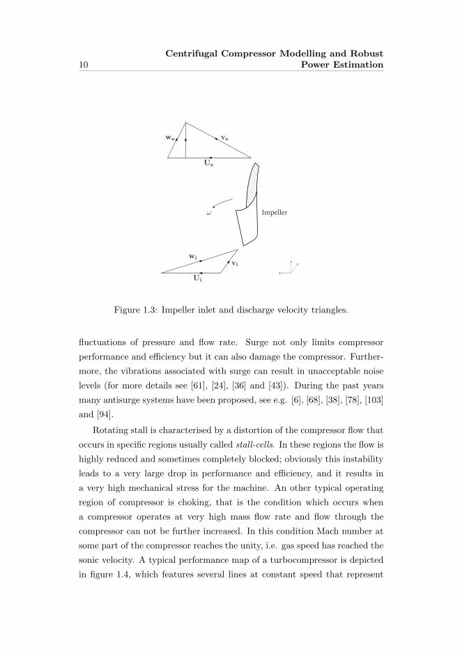
be described by using so-called velocity triangles (figure 1.3)
Centrifugal and axial flow compressors are very complex and they are
characterised by high non-linearities; moreover, they are subject to two dis-
tinct aerodynamic instabilities, rotating stall and surge, which can severely
limit the compressor performance. Surge is an unstable operating mode of
a compression system that occurs at low mass flows. It is a dynamic insta-
bility that develops into a limit cycle1 that finally results in large amplitude
1A limit cycle is a closed and periodic orbit in phase space [89].
10Centrifugal Compressor Modelling and Robust
Power Estimation
4 1 INTRODUCTION
ω Impeller
vi
Ui
wi
ve
Ue
we
Figure 1.2 / Impeller inlet and discharge velocity triangles.
Using thementioned parameters, the performance of a compressor can be graphically de-picted in a so-called compressor map. An example is shown in Figure 1.3. The individualcharacteristic curves or speed lines are formed by steady-state operating points with thesame rotational speed. The achievable flow rates are limited by the occurrence of surge atlow flows and the phenomenon known as choking at high flows. Choking occurs whenthe local velocity, usually in the impeller exit or diffuser, reaches the speed of sound. Forcompleteness also a characteristic curve for the load of the compression system is plottedin the upper part of the figure. This curve represents the total flow resistance of the sys-tem that the compressor must supply with pressurized fluid. The intersection of a speedline with the load characteristic determines the operating point of the compressor that,ideally, coincides with the point of maximum efficiency.
1.2.2 Industrial centrifugal compressors
In this thesis we focus on industrial scale centrifugal compression systems that are typ-ically used in offshore oil and gas production, (petro-)chemical process plants, and ingas transportation networks. Some typical compressor configurations are depicted inFigures 1.4 and 1.5. Important characteristics of these types of centrifugal compressorsare the large pressure rises and flow rates involved, see also Table 1.1. In order to reachthese numbers, the compressors have large diameter impellers or operate at high speedsand they consume considerable amounts of power (order of magnitude up to 10 MW),resulting in bulky machines that can withstand the large mechanical loads involved.
Figure 1.3: Impeller inlet and discharge velocity triangles.
fluctuations of pressure and flow rate. Surge not only limits compressor
performance and efficiency but it can also damage the compressor. Further-
more, the vibrations associated with surge can result in unacceptable noise
levels (for more details see [61], [24], [36] and [43]). During the past years
many antisurge systems have been proposed, see e.g. [6], [68], [38], [78], [103]
and [94].
Rotating stall is characterised by a distortion of the compressor flow that
occurs in specific regions usually called stall-cells. In these regions the flow is
highly reduced and sometimes completely blocked; obviously this instability
leads to a very large drop in performance and efficiency, and it results in
a very high mechanical stress for the machine. An other typical operating
region of compressor is choking, that is the condition which occurs when
a compressor operates at very high mass flow rate and flow through the
compressor can not be further increased. In this condition Mach number at
some part of the compressor reaches the unity, i.e. gas speed has reached the
sonic velocity. A typical performance map of a turbocompressor is depicted
in figure 1.4, which features several lines at constant speed that represent

1.1 General description 11
steady-state operating points at the same speed and two critical lines, surge
line (low flow rate) and choke line (high flow rate). These two curves are
obtained by joining respectively the surge and choke points at different con-
stant speeds, and the operating point is supposed to stay within the region
delimited by these curves.1.2 CENTRIFUGAL COMPRESSION SYSTEMS 5
Flow rate
Flow rate
Pressure
rise
surgeregion
choked flowregion
increasingspeed
Efficien
cy increasingspeed
Figure 1.3 / Illustrative compressor map with constant speed lines (black) and load char-acteristic (gray).
Furthermore, the required pressure rise is seldom realized with a single compressor stagesomost industrial compressors containmultiple stages in series, resulting in complicatedmechanical and aerodynamic designs, see also Figures 1.4 and 1.5a. In particular wemention the additional ducting that is required to guide the flow from one stage to theother. We point out that in some cases multiple compressors need to operate in series orparallel to realize the required pressure rise or flow.
Another characteristic for industrial compression systems is that they are usually inte-grated into large and complex systems like, for example, a refinery or an internationalgas distribution network. Each element in such complex systems, whether it is a reactorvessel, a pipeline, an entire oil field, or a small relief valve, can influence the compressorto which it is connected.
Industrial compression systems are expensive equipment as can be deduced from theabove, which in turn makes compressors a critical component of the entire system inwhich it operates. This imposes restrictions on the equipment used in compression sys-tems and numerous trade-offs need to be made between reliability, maintenance costsand added complexity on the one hand and improvement of functionality and perfor-mance on the other hand. Hence, the added value of new technologies needs to be proventhrough extensive analysis and test programmes, prior to their application in actual com-pression systems.
Figure 1.4: Typical turbocompressor performance map (black lines) and a
realistic load characteristic (grey line).
In order to quantify the distance between the current operating point
and the surge/choke line, the following margins Msurge and M choke can be
introduced
Msurge = 100m0 − ms
m0;
M choke = 100m0 − mc
m0.
Where m0 is the actual mass flow, ms is the mass flow rate at surge line
at the same constant speed and mc is the mass flow rate at choke line at
the same constant speed. In practice, Msurge and M choke represent the
percentage horizontal distances between the current operating point and the
surge/choke line.

12Centrifugal Compressor Modelling and Robust
Power Estimation
The most famous model for approximating dynamics of deviations of
flow and pressure variables in a compressor from their nominal steady-state
values is the Moore-Greitzer model ([66], [67] and [84]): many different ap-
proaches have been proposed in order to estimate the parameters on which
this method is based on ([70], [96]). Furthermore, many variations of Moore-
Greitzer model have been introduced to adapt this model to the requirements
of particular applications ([28] and [97]). In addition, other kind of compres-
sor models and parameters identification have been addressed in the past
years, as shown in [105] and [71].
1.2 Mathematical model for power estimation
As shown in [21], an accurate model is important to design and optimise
the control of centrifugal compressors. A typical turbo-compression train
may consist of a gas turbine (GT), which incorporates an axial compressor
used to provide high-pressure and high-density air to subsequent combustion
and expansion stages, coupled to a centrifugal compressor used to perform
mechanical work on a process gas to be compressed. This process gas has
not to be confused with the gas fueling the GT, indeed they are different
and separated gases and they never mix each other.
The work presented in this section aims to provide a reliable algorithm to
estimate the power absorbed by a CC driven by a GT. This algorithm would
provide an alternative way to estimate the GT power which is not based on
a GT model that exploits the measurements provided by the sensors all over
the GT (for instance pressure, temperature and speed transducers).
The main idea is that the power of the gas turbine is equal to the sum
of the power absorbed by the driven system and the power losses. When
the GT drives an electric generator the power can be easily estimated, in-
deed the voltage and current measurements on the electric generator allow
an extremely accurate estimation of the electric power and the losses are
negligible. When the GT drives a mechanical system as a centrifugal com-
pressor the same idea can be exploited; thus, an alternative estimation of the

1.2 Mathematical model for power estimation 13
GT power can be achieved considering the measurements on the centrifugal
compressor. However, for the time being the accuracy of sensors installed
on centrifugal compressor is not comparable to the one achievable in the
generator-drive case, which can also rely on a very realistic mathematical
model.
First of all it is necessary to introduce an high level mathematical de-
scription of the compressor, possibly irrespective of the compressor under
consideration: thus the modelling approach has to be based on a generic
centrifugal compressor structure, as the one showed in figure 1.5. Note that
the subscripts “s” and “d” simply state that the quantity refers respectively
to compressor suction (inlet) or discharge (outlet).
5 Ge Confidential
CC Model, Power Estimation Methods
The proposed algorithm should provide the required power estimation irrespective of the compressor
under consideration, thus it has to be based on a generic centrifugal compressor structure, as the one
showed below.
The schematic shown in the previous figure contains six sensors:
1. 𝑇𝑠 and 𝑇𝑑 are respectively the suction and the discharge temperature of the compressor;
2. 𝑝𝑠 and 𝑝𝑑 are respectively the suction and the discharge pressure of the compressor;
3. 𝑁 is the compressor shaft speed, typically measured by a toothed wheel;
4. ∆𝑝 is the differential pressure across a calibrated orifice, it can be taken at suction or at discharge
and it allows the evaluation of the mass flow throughout the compressor.
= 𝑘𝐹𝐸 ⋅ √Δ𝑝 ⋅ 𝜌
Where 𝜌 is the density of the gas and 𝑘𝐹𝐸 is the coefficient of the flow element. The density 𝜌 is equal to:
𝜌 =𝑀𝑤 ⋅ 𝑝
𝑍 ⋅ 𝑅 ⋅ 𝑇
Once that the mass flow is known the volumetric flow 𝑄𝑣 can be computed as follows:
𝑄𝑣 =
𝜌= 𝑘𝐹𝐸 ⋅ √
Δ𝑝
𝜌
Actually, the only measurements listed above are not sufficient to estimate the CC power: the gas
composition has to be known and it is assumed to be constant during the operation.
𝑁
𝑇𝑠 𝑝𝑠
Δp𝑠
𝑇𝑑 𝑝𝑑
Figure 1.5: Centrifugal compressor schematic.
Table 1.1 summarises the characteristic quantities needed to describe
the compressor and the nomenclature that will be used hereafter to refer to
them.

14Centrifugal Compressor Modelling and Robust
Power Estimation
Symbol Unit Definition
D [m] Impeller diameter
hp [J · kg−1] Polytropic specific head
ηp [ ] Polytropic efficiency
∆h [J · kg−1] Compressor specific head
N [rpm] Compressor speed
u [m · s−1] Impeller tip speed
Z [ ] Gas compressibility
p [kPa] Gas pressure
T [K] Gas temperature
Mw [kg ·mol−1] Molar mass
R [J · (K ·mol)−1] Gas constant
ρ [kg ·m−3] Gas density
m [kg · s−1] Mass flow
n [ ] Polytropic exponent
kv [ ] Isentropic volume exponent
kFE [ ] Flow coefficient
a [m · s−1] Sound speed
Q [m3 · s−1] Volumetric flow
v [m3 · kg−1] Specific volume
Table 1.1: Centrifugal compressor quantities nomenclature
The schematic shown in figure 1.5 is based on the measurements provided
by six sensors:
1. Ts and Td are respectively the suction and the discharge temperature
1.2 Mathematical model for power estimation 15
of the compressor;
2. ps and pd are respectively the suction and the discharge pressure of
the compressor;
3. N is the compressor shaft speed, typically measured by one or more
toothed wheels;
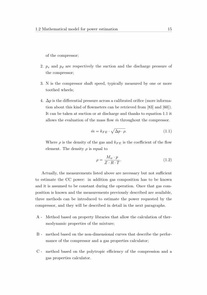
4. ∆p is the differential pressure across a calibrated orifice (more informa-
tion about this kind of flowmeters can be retrieved from [83] and [60]).
It can be taken at suction or at discharge and thanks to equation 1.1 it
allows the evaluation of the mass flow m throughout the compressor.
m = kFE ·√
∆p · ρ. (1.1)
Where ρ is the density of the gas and kFE is the coefficient of the flow
element. The density ρ is equal to
ρ =Mw · pZ ·R · T
. (1.2)
Actually, the measurements listed above are necessary but not sufficient
to estimate the CC power: in addition gas composition has to be known
and it is assumed to be constant during the operation. Once that gas com-
position is known and the measurements previously described are available,
three methods can be introduced to estimate the power requested by the
compressor, and they will be described in detail in the next paragraphs.
A - Method based on property libraries that allow the calculation of ther-
modynamic properties of the mixture;
B - method based on the non-dimensional curves that describe the perfor-
mance of the compressor and a gas properties calculator;
C - method based on the polytropic efficiency of the compression and a
gas properties calculator.
16Centrifugal Compressor Modelling and Robust
Power Estimation
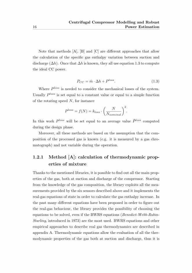
Note that methods [A], [B] and [C] are different approaches that allow
the calculation of the specific gas enthalpy variation between suction and
discharge (∆h). Once that ∆h is known, they all use equation 1.3 to compute
the ideal CC power.
PCC = m ·∆h+ P loss. (1.3)
Where P loss is needed to consider the mechanical losses of the system.
Usually P loss is set equal to a constant value or equal to a simple function
of the rotating speed N , for instance
P loss = f(N) = kloss ·(
N
Nnominal
)2
.
In this work P loss will be set equal to an average value P loss computed
during the design phase.
Moreover, all these methods are based on the assumption that the com-
position of the processed gas is known (e.g. it is measured by a gas chro-
matograph) and not variable during the operation.
1.2.1 Method [A]: calculation of thermodynamic prop-
erties of mixture
Thanks to the mentioned libraries, it is possible to find out all the main prop-
erties of the gas, both at suction and discharge of the compressor. Starting
from the knowledge of the gas composition, the library exploits all the mea-
surements provided by the six sensors described above and it implements the
real-gas equations of state in order to calculate the gas enthalpy increase. In
the past many different equations have been proposed in order to figure out
the real-gas behaviour, the library provides the possibility of choosing the
equations to be solved, even if the BWRS equations (Benedict-Webb-Rubin-
Starling, introduced in 1973) are the most used. BWRS equations and other
empirical approaches to describe real gas thermodynamics are described in
appendix A. Thermodynamic equations allow the evaluation of all the ther-
modynamic properties of the gas both at suction and discharge, thus it is

1.2 Mathematical model for power estimation 17
possible to evaluate the specific gas enthalpy increase between suction and
discharge (specific compressor head)
∆h = hd − hs. (1.4)
Beyond the accuracy of this method with respect to real power (this topic
will be discussed in section 1.2.4), it is necessary to analyse some statistical
features of this method. Considering that this method takes as inputs some
measurements provided by real sensors, it is necessary to take into account
the fact that these measurements are not ideal. This is the reason why it is
necessary to test the sensitivity of every estimation method with respect to
its own inputs. This sensitivity test quantifies the robustness of the estima-
tion method with respect to the inputs variability. The real measurements
can be statistically described by a Gaussian distribution with mean value µ
equal to the value provided by the sensor and standard deviation σ connected
with the sensor precision (retrievable from specific sensors datasheets). The
95% confidence interval of this measurement is equal to µ±2σ, while the 99%
confidence interval will be equal to µ±3σ. Detailed description about Gaus-
sian distribution can be found in [92]. The sensitivity test can be performed
adding a noise-vector (in this work 1000 elements) with proper statistical
features to every single input. After that the estimation method has to be
applied to each single case and the results can be compared with the ideal
estimation relative to zero-noise case. The Additive White Gaussian Noises
(AWGN) relative to each input have been defined as follows.
• To define the mean value of each measurements a real trend has been
taken into consideration;
• concerning pressure sensors, the standard deviation is set equal to σ =
0.125% of the measurement range (95% confidence interval, i.e. [µ −2σ;µ+ 2σ], corresponds to 0.25% of the measurement range);
• flow-meters are based on the measurements of pressure across an ori-
fice. Their standard deviation is set equal to 0.5% of the measurement

18Centrifugal Compressor Modelling and Robust
Power Estimation
range (95% confidence interval, i.e. [µ−2σ;µ+2σ], corresponds to 1%
of the measurement range);
• thermocouples datasheets usually provide a rectangular distribution to
statistically describe the measurements. If the rectangular distribution
has amplitude 2B it is possible to prove that the standard deviation
of the correspondent Gaussian distribution is σ = B√3.
Figure 1.6 shows an histogram of the percentage difference between noised
inputs power estimation based on method [A] and the CC power computed
with no-noise inputs.
-8 -6 -4 -2 0 2 4 6 8
Diff [%]
0
20
40
60
80
100
120
N
Figure 1.6: Deviation with respect to case without noise using method [A]
(µ = −0.02%, σ = 1.92%).
1.2.2 Method [B]: non-dimensional curves
As described in [61] and [24], the behaviour of a centrifugal compressor can
be characterised using non-dimensional quantities ϕ and τ , i.e. adimensional

1.2 Mathematical model for power estimation 19
variables defined as follows
τ =∆h
u2; (1.5)
ϕ =4QsπD2u
=4kFE
√∆pρ
πD2u. (1.6)
Where Qs is the volumetric flow at suction defined as
Qs =m
ρ=kFE√
∆p · ρρ
= kFE
√∆p
ρ.
The impeller tip speed u can be computed starting from the rotating speed
N and the impeller diameter D as
u =πND
60.
These are experimental maps that describe the operating points where the
compressor is able to work, and they are defined at first during the design
phase (Expected maps) and then they are corrected to match the particular
behaviour of each single machine with proper tests (As-Tested maps). Each
map is defined as a family of curves obtained with different value of Mach
number M , defined as the ratio between the impeller tip speed u and the
sound speed in that thermodynamic conditions a
M =u
a=
u√kvZRTMw
. (1.7)
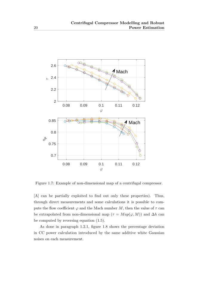
Figure 1.7 shows an example of non-dimensional map: note that usually
these representations include a map relative to τ and a map relative to the
polytropic efficiency ηP , even if in this method [B] only the τ map is required.
Equation (1.7) relies on the knowledge of some gas properties, such
as gas compressibility Z (real gas behaviour is described by the equation
pvMw = ZRT , see appendix A), isentropic volume exponent kv and molecu-
lar weight Mw. This means that such method needs a suitable algorithm for
the definition of these quantities (e.g. the libraries introduced with method
20Centrifugal Compressor Modelling and Robust
Power Estimation
0.08 0.09 0.1 0.11 0.122
2.2
2.4
2.6
0.08 0.09 0.1 0.11 0.12
0.7
0.75
0.8
0.85
P
Mach
Mach
Figure 1.7: Example of non-dimensional map of a centrifugal compressor.
[A] can be partially exploited to find out only these properties). Thus,
through direct measurements and some calculations it is possible to com-
pute the flow coefficient ϕ and the Mach number M , then the value of τ can
be extrapolated from non-dimensional map (τ = Map(ϕ,M)) and ∆h can
be computed by reversing equation (1.5).
As done in paragraph 1.2.1, figure 1.8 shows the percentage deviation
in CC power calculation introduced by the same additive white Gaussian
noises on each measurement.

1.2 Mathematical model for power estimation 21
-6 -4 -2 0 2 4 6
Diff [%]
0
50
100
150
N
Figure 1.8: Deviation with respect to case without noise using method [B]
(µ = −0.23%, σ = 1.51%).
1.2.3 Method [C]: compressor polytropic efficiency
This method is based on the polytropic efficiency of the centrifugal com-
pressor ηP ∈ (0; 1), defined as the ratio between the ideal polytropic specific
head ∆hP required to compress the gas and the real one ∆h
ηP =∆hP∆h
. (1.8)

22Centrifugal Compressor Modelling and Robust
Power Estimation
It is possible to demonstrate2 that the polytropic head is equal to
∆hP =Zs ·R · Ts
Mw·
(pdps
)σ− 1
σ. (1.9)
Method [C] follows these steps to compute ∆h:
i. A gas properties calculator (e.g. the one described in paragraph 1.2.1)
provides the value of X, Y and kv, both at suction and discharge
(respectively subscript “s” and “d”)
X =
(∂Z
∂T
)p
T
Z,
Y = 1− p
Z
(∂Z
∂p
)T
,
kv = isentropic volume exponent;
ii. polytropic efficiency ηP can be retrieved by interpolation of the ηP
non-dimensional curves (similar to the map represented in figure 1.7)
ηP = Map(ϕ,M);
iii. the coefficient σ has to be computed both at suction and discharge,
thanks to the relationship
σ =n− 1
n=kv − 1
kv·X + 1
ηP
1 +X+
1− Y1 +X
·(
1− 1
ηP
); (1.10)
2A polytropic process follows the relation pvn = C, where n is the polytropic expo-
nent([61]). Thus, it is possible to write these relationships
pvn = psvns ; =⇒ v = vs
(ps
p
) 1n
;
Since ∆hP =∫ ds vdp, it follows that
∆hP =
∫ d
svdp = vsp
1ns
∫ pd
ps
p−1n dp = psvs
n
n− 1
[(pd
ps
)n−1n
− 1
].
Considering that pvMw = ZsRTs, and defining σ = n−1n
we obtain
∆hP =ZsRTs
Mw
1
σ
[(pd
ps
)σ− 1
].

1.2 Mathematical model for power estimation 23
Equation (1.10) clearly states that σ is a function of ηP . Then, the
average coefficient σ is equal to
σ =σs + σd
2. (1.11)
Finally, merging equations 1.8 and 1.9 it is possible to find out ∆h.
∆h =1
ηP
Zs ·R · TsMw
·
(pdps
)σ− 1
σ. (1.12)
As done in paragraph 1.2.1 and 1.2.2, figure 1.9 shows the percentage
deviation in CC power calculation introduced by the same additive white
Gaussian noises on each measurement.
-10 -5 0 5 10
Diff [%]
0
50
100
150
N
Figure 1.9: Deviation with respect to case without noise using method [C]
(µ = −0.28%, σ = 2.71%).
1.2.4 CC power estimation: results
Sensitivity analysis
As shown in figure 1.6, 1.8 and 1.9 all the three methods preserve the Gaus-
sian shape, with a mean value µ very close to 0. Nevertheless, the same de-

24Centrifugal Compressor Modelling and Robust
Power Estimation
viations on the inputs do not lead to similar deviations on power estimations
and this is due to the fact that different methods have different sensitivity
with respect to the same inputs. Table 1.2 summarises the results of the
sensitivity analysis. Table 1.2 states that method [C] is statistically more
sensitive with respect to input noises, thus the centrifugal compressor power
estimation provided by this method is the most affected by the inaccuracy
of input measurement.
µ σ
method [A] −0.02% 1.92%
method [B] −0.23% 1.51%
method [C] −0.28% 2.71%
Table 1.2: Outcomes of sensitivity analysis of methods [A], [B] and [C].
Estimation error
Sensitivity analysis describes how the results are conditioned by inputs vari-
ations, but it is not enough to evaluate the quality of the estimation method.
In order to assess the accuracy of the three methods it is necessary to feed
each method with real field data and compare the results with the power
measurement provided by a suitable field device. In turbo-compression in-
dustrial applications, like the one under investigation, a direct power mea-
surement system is not usually needed; nevertheless, when it is strictly re-
quired3, torque-meters are commonly used (to retrieve more details about
torque-meters please refer to [93]). It is worth noticing that this transducer
is affected by great inaccuracies (up to 10% in case of wrong calibration),
thus the errors defined with respect to this measurement have to be weighted
under the light of accuracy of each particular transducer. This is due to the
3 In some country LNG plants (Liquefied Natural Gas) are obliged by law to measure
and declare the absorbed power for tax purposes.

1.2 Mathematical model for power estimation 25
nature of torque-meters, indeed the quality of the measurements is strictly
connected with a correct calibration phase. As shown in figure 1.10, the
torque measurement is indirectly achieved by evaluating the angular dis-
placement ∆ϑ between the extremities of the torque-meter; indeed, consid-
ering that the instrument has an equivalent torsional stiffness equal to K,
when the torque-meter is excited with a torque T then ∆ϑ should be equal
to T/K. Coefficient K obviously is not constant and varies with different
factors (for instance a temperature compensation is usually needed), and
this is the reason why calibration procedures are so important.
Figure 1.10: Generic schematic of a torque-meter.
Figure 1.11 shows some results obtained by exploiting four different
datasets taken from real sites (Tscan = 1280ms). These plots represent the
percentage difference between the power value provided by torque-meter and
the power estimation based respectively on method [A] (blue line), method
[B] (orange line) and method [C] (yellow line).

26Centrifugal Compressor Modelling and Robust
Power Estimation
0 1000 2000 3000 4000 5000 6000 7000 8000Time [s]
-6
-4
-2
0
2
Diff
[%]
0 1000 2000 3000 4000 5000 6000 7000 8000Time [s]
-10
-5
0
Diff
[%]
0 500 1000 1500 2000 2500 3000 3500Time [s]
-10
0
10
Diff
[%]
0 500 1000 1500 2000 2500 3000 3500Time [s]
-8
-6
-4
-2
0
Diff
[%]
Figure 1.11: Percentage errors of centrifugal compressor power estimation
based on method [A] (blue line), method [B] (orange line) and method [C]
(yellow line).

1.2 Mathematical model for power estimation 27
Results of figure 1.11 have been confirmed repeating the estimation with
other trends, and they can be summarised as follows:
i. Different tests lead to different errors, therefore the errors are not only
due to the methods but they are in some way connected to the char-
acteristics and non-idealities of the particular site setup.
ii. Despite the absolute value of the errors, all the three methods are char-
acterised by a nearly constant percentage error. Considering that the
measured power undergoes significant variation within the estimation
interval, this means that each estimation method features a constant
bias with respect to the reference. Standing from the inaccuracy that
might affect the torque-meter this is a very appreciable feature;
iii. Method [A], which is based only on gas properties and transforma-
tions, seems to guarantee better results. However, it is worth noticing
that methods [B] and [C] rely on non-dimensional map, and these re-
sults are based on Expected Maps, thus they do not take into account
the peculiarities of each machine as As-Tested maps do. As already
mentioned, Expected maps are ideal compressor maps computed during
the design phase of the CC, while As-Tested maps are real compres-
sor maps confirmed by tests and measurements taken on CC in real
operating conditions and various operating points.
1.2.5 Method [C2]: compressor polytropic efficiency with
model-based correction
This additional method is very similar to method [C], but it introduces a
correction based on the analytical prediction of discharge temperature Td
based on the theory of polytropic compression
Td = Ts ·
(pdps
)σ(ηP )
. (1.13)

28Centrifugal Compressor Modelling and Robust
Power Estimation
Equation (1.13) can be easily retrieved starting from the definition of σ
σ =
ln
(TdTs
)ln
(pdps
) , (1.14)
that directly derives from the thermodynamic theory of a polytropic expan-
sion or compression4.
The main idea behind this method [C2], as shown in figure 1.12, is to
find out the value of polytropic efficiency ηP that makes the predicted value
of discharge pressure to coincide with the measured one, i.e.
Td(ηP ) = Tmeasd .
This method [C2] could also be based on the prediction of pd; indeed,
an equation similar to (1.13) can be derived concerning pd. However, by
construction, the value ηP that would make pd to match with the measured
value pd is exactly the same value obtained exploiting the prediction of the
discharge temperature.
4 A polytropic expansion follows this pressure-temperature relationship (for a complete
proof see [61])
pn−1
Tn= C,
where n is the polytropic exponent and C a constant. This means that for an arbitrary
compression the following equation is satisfied
pn−1n
d
Td=pn−1n
s
Ts.
It is possible to demonstrate that the quantity σ = n−1n
is a function of the polytropic
efficiency ηP , thus
σ(ηP ) =n− 1
n=γ − 1
γηP,
where γ =cpcv
. Finally, we obtain the desired relationship
Td
Ts=
(pd
ps
)σ(ηP )
.

1.2 Mathematical model for power estimation 29
1 Ge Confidential
𝑇𝑑 𝑚𝑒𝑎𝑠𝑢𝑟𝑒𝑑 𝑁
∆𝑃𝑑
𝑃𝑑
𝑃𝑠
𝑇𝑑
𝑇𝑠
𝜂𝑃
∆𝜂𝑃
+ +
- + 𝑇𝑑(𝜂Ƹ𝑃)
𝑝𝑜𝑤𝑒𝑟_𝑒𝑠𝑡(𝜂Ƹ𝑃)
𝛴𝜂𝑃
𝑘 න(∙)𝑑𝜏
𝑡
0
𝜂𝑃 non-dimensional
Map
𝜂Ƹ𝑃
Figure 1.12: Schematic of method [C2].
Method [C2]: results
Figure 1.13 features the results of method [C2] (orange line) and method
[C] (blue line). Note that the method has been applied to the same four
datasets relative to figure 1.11.

30Centrifugal Compressor Modelling and Robust
Power Estimation
0 1000 2000 3000 4000 5000 6000 7000 8000Time [s]
-4
-2
0
2
4
Diff
[%]
0 1000 2000 3000 4000 5000 6000 7000 8000Time [s]
-4
-2
0
2
4
Diff
[%]
0 500 1000 1500 2000 2500 3000 3500Time [s]
0
2
4
6
Diff
[%]
0 500 1000 1500 2000 2500 3000 3500Time [s]
-6
-4
-2
0
2
Diff
[%]
Figure 1.13: Percentage errors of centrifugal compressor power estimation
based on method [C] (blue line) and method [C2] (orange line).

1.3 Robustness with respect to measurements 31
Even in this case it does not seem possible to define a general behaviour
pattern of this method, however method [C2] generally guarantee better
results with respect to method [C]. Furthermore, figure 1.13 clearly shows
that the percentage errors relative to method [C2] are usually characterised
by an initial transient phase due to the time needed by ∆ηP to converge to
a nearly constant value.
The reason of the improvement introduced with method [C2] is the fact
that the polytropic efficiency is not retrieved only from a scheduled map,
indeed it is corrected thanks to direct measurement of discharge temperature
Td.
1.3 Robustness with respect to measurements
All the power estimation methods presented in section 1.2 rely on some of the
six sensors represented in figure 1.5; obviously not all the methods exploit
all the six measurements, but the point now is that every method needs to
be fed by inputs provided by some kind of sensors.
Thus, the question is: how is it possible to improve the robustness of a
generic estimation method with respect to one or more of these six measure-
ments? Let’s suppose that one of the six measurements suddenly becomes
unavailable; is it possible to compensate this information leakage by using
the remaining five, or all the measurements are strictly required? These ques-
tions do not have specific answers, indeed some measurements are strictly
necessary to keep the system working. For instance, rotating speed mea-
surements are very important, thus a typical industry setup includes two or
three transducers to guarantee the redundancy of this basic measurement.
Rotating speed awareness is so important that it does not make any sense
to suppose the unavailability of this measurement, indeed in that case the
system would automatically shut down.
On the other hand, sometimes there are other sensors that are very useful
even if they are not essential. Concerning the proposed methods introduced
to estimate the power needed to drive a centrifugal compressor, it would be
32Centrifugal Compressor Modelling and Robust
Power Estimation
very appreciable to find out some techniques to make the system able to
turn around the temporary unavailability of a sensor. To reach this aim two
main techniques have been investigated:
• A technique exclusively based on Recursive Least Squares theory (RLS,
see section B.2 in appendix B);
• A technique based both on thermodynamic formulae and RLS theory.
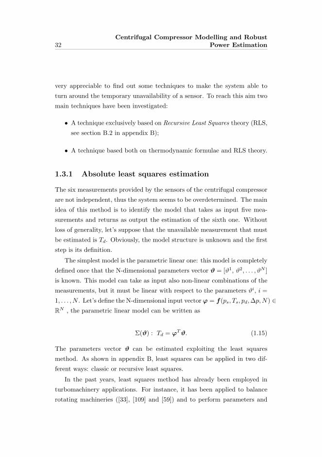
1.3.1 Absolute least squares estimation
The six measurements provided by the sensors of the centrifugal compressor
are not independent, thus the system seems to be overdetermined. The main
idea of this method is to identify the model that takes as input five mea-
surements and returns as output the estimation of the sixth one. Without
loss of generality, let’s suppose that the unavailable measurement that must
be estimated is Td. Obviously, the model structure is unknown and the first
step is its definition.
The simplest model is the parametric linear one: this model is completely
defined once that the N-dimensional parameters vector ϑ = [ϑ1, ϑ2, . . . , ϑN ]
is known. This model can take as input also non-linear combinations of the
measurements, but it must be linear with respect to the parameters ϑi, i =
1, . . . , N . Let’s define the N-dimensional input vectorϕ = f(ps, Ts, pd,∆p,N) ∈RN , the parametric linear model can be written as
Σ(ϑ) : Td = ϕTϑ. (1.15)
The parameters vector ϑ can be estimated exploiting the least squares
method. As shown in appendix B, least squares can be applied in two dif-
ferent ways: classic or recursive least squares.
In the past years, least squares method has already been employed in
turbomachinery applications. For instance, it has been applied to balance
rotating machineries ([33], [109] and [59]) and to perform parameters and

1.3 Robustness with respect to measurements 33
coefficients identification in centrifugual compressors ([76]) or in turbine en-
gines ([65] and [12]). In this framework least squares are applied in a different
way, indeed the main purpose is to find out how different CC measurements
are connected between each other.
Hereafter recursive least squares (RLS) will be used, indeed such method
updates the estimation step by step and it converges exactly to the same
result of classic least squares. Since the model is linear, an analytical solu-
tion can be defined. Obviously, to perform the least squares method, the
measurement of the variable that has to be estimated at least in a first phase
must be available. Once that the parameters vector has been estimated, if
the measurement becomes unavailable it can be estimated introducing ϑ in
the parametric linear model.
This simple idea is represented in figure 1.14: clearly the loop is closed
only when Td is available, otherwise the system works in open-loop and the
estimation Td is based on the last estimation of ϑ.
33 Ge Confidential
Least squares estimation
The six measurements provided by the sensors of the centrifugal compressor are not independent. The
main idea of this method is to identify the model that takes as input five measurements and returns as
output the estimation of the sixth one. For instance, let suppose that the unavailable measurement that
must be estimated is 𝑇𝑑.
Obviously, the model structure is unknown and the first step is its definition. The simplest model is the
parametric linear one: this model is completely defined once that the parameters vector 𝝑 =
[a1 … an] is known. This model can take as input also non-linear combination of the measurements,
but it must be linear with respect to the parameters 𝑎𝑖 . Let define the input vector 𝝋 =
𝒇(𝑇𝑠, 𝑝𝑠, 𝑝𝑑 , ∆𝑝, 𝑁), the parametric linear model can be written as:
𝛴(𝝑) ∶ 𝑑 = 𝝋′𝝑
The parameters vector 𝝑 can be estimated exploiting the least squares method. Since the model is linear,
an analytical solution can be defined. Obviously, to perform the least squares method, the measurement
of the variable that has to be estimated (in this case 𝑇𝑑) at first must be available. Once that the
parameters vector has been estimated, if the measurement becomes unavailable it can be estimated
introducing in the parametric linear model.
The least squares method can be applied in different ways. The first one (Classic Least Squares) takes into
account the data acquired within a fixed temporal window, thus the estimation is constant inside a
window and it is updated when a new window is totally acquired. On the contrary, the second one
_
Estimation
error
-
+
𝑇𝑑
Parametric
Linear Model
𝛴(𝝑)
𝑝𝑠
𝑇𝑠
𝑝𝑑
∆𝑝
𝑁
𝑇𝑑
Least
squares
method
Figure 1.14: Schematic of Td absolute estimation based on least squares
theory.

34Centrifugal Compressor Modelling and Robust
Power Estimation
In order to simulate this scenario a real dataset has been split in two sep-
arated phases. In the former part (10% of total data) all the measurements
are considered available, thus within this interval it is possible to compute
vector ϑ. In the latter interval (last 90% of data) Td is considered unknown
and it is estimated using the least squares theory.
Obviously this procedure can be repeated for each measurement, thus
each quantity will have its own coefficient vector.
Figure 1.15 is composed of five subplots relative to these tests:
1. y = Ts, ϕ = [ps Td pd ∆p N ];
2. y = ps, ϕ = [Ts Td pd ∆p N ];
3. y = Td, ϕ = [Ts ps pd ∆p N ];
4. y = pd, ϕ = [Ts pd Td ∆p N ];
5. y = ∆p, ϕ = [Ts ps Td pd N ];

1.3 Robustness with respect to measurements 35
1000 2000 3000 4000 5000 6000 7000Time [s]
-0.5
0
0.5
Ts e
rr [%
]
0 1000 2000 3000 4000 5000 6000 7000 8000Time [s]
-202
ps e
rr [%
]
0 1000 2000 3000 4000 5000 6000 7000 8000Time [s]
-0.2
0
0.2
Td e
rr [%
]
0 1000 2000 3000 4000 5000 6000 7000 8000Time [s]
-1
0
1
pd e
rr [%
]
0 1000 2000 3000 4000 5000 6000 7000 8000Time [s]
-4-2024
p e
rr [%
]
Figure 1.15: Percentage errors of absolute estimations based on least squares
theory. Blue line (10% of total data) refers to calibration phase, while orange
line (last 90% of data) refers to validation interval.

36Centrifugal Compressor Modelling and Robust
Power Estimation
1.3.2 Thermodynamic prediction and RLS estimation
Gas compression can be completely described from a physical point of view.
Equation (1.14) is valid for a polytropic process and by the inversion of this
equation it is easy to achieve an analytic formulation for the thermodynamic
prediction of Ts, ps, Td and pd.
Ts = Td ·
(pspd
)σ; (1.16)
ps = pd ·
(TsTd
) 1σ
; (1.17)
Td = Ts ·
(pdps
)σ; (1.18)
pd = ps ·
(TdTs
) 1σ
. (1.19)
Using these prediction formulae it is possible to achieve an estimation of
these variables. Figure 1.16 represents the results of these thermodynamic
predictions. Note that the differential pressure across the orifice can not be
estimated in this way, indeed this quantity is not involved in equation (1.14).
Figure 1.16 clearly shows that the thermodynamic predictions provide a
first approximation, but the error can be significant (up to 10%). This is due
to the non-idealities that move the real CC behaviour far away from ideal
polytropic compression. This means that the performance of this estimation
method is strictly connected with the particular features of the compressor
and its operating conditions. The more the compressor is far from the ideal
one, the larger the prediction errors will be. A great advantage of this
method is that it never relies on the measurement of the possibly unavailable
quantity, indeed it does not require any calibration phase and it achieves an
estimation exploiting only physical relationships. Even if this method does
not guarantee a great accuracy it gives however a first information, indeed
the error is nearly constant. This means that the prediction somehow follows

1.3 Robustness with respect to measurements 37
0 1000 2000 3000 4000 5000 6000 7000 8000Time [s]
-1
-0.5
0
Ts e
rr [%
]
0 1000 2000 3000 4000 5000 6000 7000 8000Time [s]
5
10
15
ps e
rr [%
]
0 1000 2000 3000 4000 5000 6000 7000 8000Time [s]
0
0.5
1
Td e
rr [%
]
0 1000 2000 3000 4000 5000 6000 7000 8000Time [s]
-6
-4
-2
pd e
rr [%
]
Figure 1.16: Percentage errors of thermodynamic predictions.

38Centrifugal Compressor Modelling and Robust
Power Estimation
the changing of the unknown variable, therefore the natural improvement is
to start from this result and try to compensate in some way the prediction
error. This can be made exploiting again RLS, as shown in figure 1.17. In this
case, the purpose of RLS is not the absolute estimation of one measurement,
but it aims to estimate the difference between the thermodynamic prediction
and the measured value.
37 Ge Confidential
This second method does not give an absolute estimation of the unavailable measurement,
indeed it takes as starting point the thermodynamic prediction and then it tries to estimate the
prediction error by the identification of the linear parametric model that describes the relation
between the input variables and the estimation error.
𝑇𝑑 prediction
𝝑
_
Estimation
error
-
+
𝑒𝑇𝑑
Parametric
Linear Model
𝛴(𝝑)
𝑒Ƹ𝑇𝑑
Least
squares
method
-
+
𝑇𝑑
Thermodynamic
formulae
𝑝𝑠
𝑇𝑠
𝑝𝑑
∆𝑝
𝑁
Figure 1.17: Schematic of Td prediction error estimation based on RLS the-
ory.

1.3 Robustness with respect to measurements 39
In practice, the idea is to estimate εTs , εps , εTd and εpd , defined as
εTs = Tmeass − Ts;
εps = pmeass − ps;
εTd = Tmeasd − Td;
εpd = pmeasd − pd.
Figure 1.18 shows that this second method leads to significantly lower errors
with respect to simple predictions. Moreover, even if the magnitudes of the
estimation errors are similar to the ones obtained with absolute RLS estima-
tion, this method deserves to be preferred because it is not only a “blind”
estimation but it starts from a reasonable results based on compression the-
ory.

40Centrifugal Compressor Modelling and Robust
Power Estimation
0 1000 2000 3000 4000 5000 6000 7000 8000Time [s]
-0.5
0
0.5
Ts e
rr [%
]
0 1000 2000 3000 4000 5000 6000 7000 8000Time [s]
-1
0
1
ps e
rr [%
]
0 1000 2000 3000 4000 5000 6000 7000 8000Time [s]
-0.5
0
0.5
Td e
rr [%
]
0 1000 2000 3000 4000 5000 6000 7000 8000Time [s]
-2
0
2
pd e
rr [%
]
Figure 1.18: Percentage errors obtained estimating the thermodynamic pre-
diction error with RLS. Blue line (10% of total data) refers to calibration
phase, while orange line (last 90% of data) refers to validation interval.

1.4 Results analysis and conclusions 41
1.4 Results analysis and conclusions
The methods proposed in this chapter have been developed to meet practical
and technological needs. Concerning typical CC applications power measure-
ment is not strictly required. On the other hand, the knowledge about GT
power is fundamental to figure out the GT operating point. Thus, consider-
ing that CCs are usually driven by GTs, the information about the absorbed
power can be exploited as GT delivered power estimator.
The power absorbed by the CC can be directly measured by torque-
meters, but such sensors have many drawbacks, indeed they are expensive,
bulky and they need to be frequently calibrated in order to guarantee ac-
ceptable accuracy. The proposed techniques provide an estimation of the
absorbed power avoiding torque-meter installation, and this is the reason
why they are so appreciable.
This chapter can be broadly split in two different parts:
i. in the first part some suitable model-based methods to estimate the
power needed to drive a centrifugal compressor have been proposed. As
mentioned in paragraph 1.2.4, methods [A], [B] and [C] lead to nearly
constant percentage error, even if different tests are characterised by
different errors. However, method [A] seems to guarantee better re-
sults, while the performances of methods [B] and [C] are strictly con-
nected to the goodness of the empirical maps that try to describe
the CC behaviour. In this framework the importance of introducing
As-Tested maps instead of Expected maps is crucial, and it can bring
many benefits. Moreover, an additional method [C2] is proposed: this
method tries to enhance method [C] by introducing a model-based
correction of the polytropic efficiency. Even in this case it is hard to
define a general pattern, indeed different datasets lead to different re-
sults. Nevertheless, method [C2] generally guarantees better results
with respect to method [C];
ii. in the second part some methods to compensate the potential unavail-
ability of some sensors are investigated. The main idea is that CC

42Centrifugal Compressor Modelling and Robust
Power Estimation
measurements taken from suction and discharge are not independent,
indeed they are linked with each other by thermodynamic relationships
that describe gas compression. The proposed methods exploit RLS
theory and thermodynamic relationships in order to achieve a suitable
estimation of the potentially unavailable measurement. Empirical re-
sults based on real trend data show that the minimum estimation error
can be achieved exploiting at the same time both the thermodynamic
predictions and RLS theory.

Chapter 2
Sub-Synchronous Torsional
Interactions in Electrical Networks
Turbo-generators (TGs) interact with electrical network and sig-
nificant torsional vibrations at shaft natural frequencies can be
produced. The first part of this chapter introduces sub-synchronous
torsional interactions, with a brief survey of the main causes and
effects of this phenomenon. The second part suggests a possible
solution to mitigate this issue and some theoretical results are
presented.
2.1 General description
SSTI (Sub-Synchronous Torsional Interaction) is an instability phenomenon
mainly associated with synchronous machines and various power electronic
devices that are widely used in oil and gas industry, such as HVDC converters
(High Voltage Direct Current) or large industrial motor drives that create
and sustain the oscillations ([90], [81], [11] and [41]). The presence of these
devices has grown exponentially in the last decade, particularly for Variable
Frequency Drive application (VFD); these equipments are mainly used in
electro-mechanical systems to control AC motor speed and torque by varying
43

44 Sub-Synchronous Torsional Interactions in Electrical Networks
motor input frequency and voltage. VFDs can produce a massive current
and voltage harmonic distortion, and this is the first step to trigger SSTI
oscillations.
SSTI as a non-linear phenomenon has been widely studied in the past
decades ([45]), and it can not be understood by considering the electrical
and mechanical parts as separated worlds: looking at these two systems
one by one the mechanical/electrical fluctuations can not be explained, they
seem to be self-generated and self-sustained oscillations. The causes and the
reasons behind this very critical behaviour of electric generation plants have
to be searched considering a single system where the electric part (electric
network and electronic devices) and the mechanical part (gas turbines and
generators) transfer energy to each other. Figure 2.1 depicts a very schematic
electric grid powered by turbo-generators (even if the grid is a three-phase
network, for the sake of simplicity the schematic is represented as a single-
line diagram).
Laboratorio di Automatica
Gruppo Dinamica Non Lineare e Controllo di Sistemi
Dipartimento di
Ingegneria dell’Informazione
M. Galanti 9 24 Ottobre 2016 Dottorato di Ricerca in Ingegneria dell’Informazione, XXXI ciclo
GT
G
GT
G
. . .
Δ-Y Δ-Y
Δ-Y
Passive
load Active
load . . .
SSTI – Sub-Synchronous Torsional Interactions
Δω→ΔV
Δi→ΔT
Electric
Network
Figure 2.1: Schematic explanation of SSTI phenomenon.
As any other rotating mechanical component, TGs have their own Tor-
sional Natural Frequencies (TNFs). Usually, the first torsional mode is dom-
inant, and in correspondence of this frequency the behaviour of the mechan-
ical system becomes very unstable. If an external source of energy feeds a
TGs in correspondence of the first TNF (1TNF) the system will begin to

2.2 SSTI electro-mechanical causes 45
oscillate with undamped vibrations. The oscillation ∆ω of the shaft line, i.e.
variations in rotational speed with respect to the reference speed, is defined
as
∆ω = ωact − ωref ,
where ωact is the actual angular speed of the shaft line, while ωref is the
reference angular speed which is directly connected to the reference frequency
of the network (50 or 60Hz). ∆ω creates voltage oscillation ∆V . Electric
network sees these voltage variations as disturbances, thus it injects in the
grid significant current oscillations ∆i. On the contrary, TGs see the current
oscillations as electric torque oscillations (∆Te), and this is the external
source of energy that excites the mechanical system exactly where it is more
sensitive, i.e. in correspondence of 1TNF. This is a very intuitive explanation
of how the SSTI phenomenon can be produced and self sustained: obviously
each single plant has its own peculiarities, and they have to be considered
in order to assess the actual SSTI risk and, possibly, its mitigation.
SSTI vibrations can cause cumulative fatigue damage and result in re-
duced component life of parts such as shafts, buckets (blades), retaining
rings, and rotors. However, in addition to physical damages on the plant,
this phenomenon heavily affects the operability of the system, indeed when
seismic sensors detect too large oscillations the system is automatically shut
down in order to protect itself and preserve the surrounding workers’ safety.
In order to avoid this critical situation SSTI causes have to be studied and
some mitigation techniques need to be introduced (e.g. see [90], [79], [52],
[85] and [91]).
2.2 SSTI electro-mechanical causes
TGs shafts have to transmit driving torque to the load (i.e. electric net-
work) and they have also to absorb the transient torque that characterises
step events or faults. As mentioned in the previous paragraph, under certain
conditions they can experience self-sustained or growing oscillations due to
SSTI. In order to find out SSTI main causes first of all it is necessary to

46 Sub-Synchronous Torsional Interactions in Electrical Networks
introduce a mechanical model of TG to better understand why the system
tends to oscillate in correspondence of specific frequencies. Then, it is nec-
essary to analyse the electric grid in order to explain why certain devices in
some configurations create disturbances that feed the torsional oscillations.
2.2.1 Turbo-generators mechanical model
The first step to explain this phenomenon is the introduction of a mathe-
matical model of TG mechanics. The modal approach (see e.g. [44], [46] and
[104]) allows the calculation of the characteristic TNFs of the train usually
composed of a GT, a gear box and an EG.
As shown in figure 2.2, TG shaft can be seen as a sequence of N in-
ertias Ji characterised by damping coefficients Di, with i = 1, · · · , N , and
interconnected by equivalent stiffness coefficients kj , j = 1, · · · , N − 1.
ϑ1 ϑ2 ϑ𝑁−1 ϑ𝑁
𝑘1𝐽1
𝑘𝑁−1 𝑇
𝐷1
𝐽2 𝐽𝑁−1 𝐽𝑁
𝐷2 𝐷𝑁−1 𝐷𝑁
Figure 2.2: Physical model of TG shaft.
The shaft torsional dynamic behaviour is completely described by the
following set of second order differential equations
Jϑ+Dϑ+Kϑ = T . (2.1)
Where:
J = diagonal matrix of physical inertias
D = diagonal matrix of physical damping coefficients
K = symmetric matrix of equivalent stiffness coefficients

2.2 SSTI electro-mechanical causes 47
ϑ = vector of angular positions of each inertia
T = torques vector (both electric and mechanical)
In a power generation system, in addition to mechanical damping there is
also an electrical damping which is acting on the generator shaft; this electri-
cal damping is linked to the electrical torque which is due to the interaction
between the network and the generator magnetic flux. In practice, consider-
ing small oscillations in correspondence of a certain frequency fn, electrical
torque and speed oscillations can be seen as rotating phasors, respectively
∆T e(fn) and ∆ω(fn).
Electrical damping acts on generator shaft windings, and it describes the
amplification and the phase delay between speed oscillations and electrical
torque. Mathematically, it is defined as
De(fn) = −|∆T e(fn)||∆ω(fn)|
cosα, (2.2)
where α is the phase delay between the phasors. De obviously depends on α
and it can be either positive or negative. Since the total damping coefficient
is a combination of the mechanical and electrical damper coefficients, it is
clear that a negative De can lead the system towards instability.
The drawback of equation (2.1) is that it is very complex to figure out
the numerical values of its coefficients. In order to overcome this issue it
is possible to represent the same equation in the modal reference system
through this coordinate transformation
ϑ = Φ · q. (2.3)
Where:
Φ = modal shapes matrix (calculated as the eigenvectors of J−1K)
q = modal coordinates vector
Theory fundamentals about modal analysis can be found in many hand-
books such as [5], [86] or [69].
By applying this transformation, equation (2.1) becomes
M eqq +Deqq +Keqq = T eq. (2.4)

48 Sub-Synchronous Torsional Interactions in Electrical Networks
Where:
M eq = ΦTJΦ is a diagonal matrix
Deq = ΦTDΦ is a diagonal matrix
Keq = ΦTKΦ is a diagonal matrix
Solving this new set of differential equations it is possible to figure out all
torsional modes relative to each single TNF. The major criticality is related
to the first mode, thus it is reasonable to focus the attention only on 1TNF,
which considering common size and inertias in practical applications in the
oil and gas industry usually is lower than 10Hz. The normalised amplitude
of this first torsional mode gives a first quantitative information on how the
mechanical system amplifies the torque/speed oscillations at 1TNF. Torque
and speed oscillations are linearly connected by equivalent stiffness, thus if
one gets larger also the other one is amplified by the same factor.
Therefore, the higher is this amplification the lower will be the total
equivalent damping coefficient; this is due to the fact that if the electric
torque is more amplified in correspondence of generator windings then the
electric damping coefficient has a greater weight in the calculation. In some
cases the amplitude of the first torsional mode is particularly large, thus the
total equivalent damping coefficient can be lower than 0, and this means
that the system is not able to damp the oscillations with frequency equal to
1TNF, thus the stability is not guaranteed.

2.3 Harmonic distortion in the electric network 49
2.3 Harmonic distortion in the electric net-
work
It is well-known that a three-phase electric power transmission and distri-
bution system is theoretically characterised by a balanced and symmetric
configuration, where each line carries an alternating current of the same fre-
quency f and amplitude I; the reason why the system is perfectly balanced
is that in the phase plane the three phase currents present a phase delay
equal to 2π/3, and this forces the sum of the three currents to zero. Obvi-
ously, also the three line voltages have the same amplitude V and the same
frequency f , and they are delayed each other in the phase plane of 2π/3.
Indicating with “a”, “b” and “c” each line, equations (2.5) and (2.6) describe
the ideal currents and voltages of a symmetric three-phase system.va(t) = V sin(2πft);
vb(t) = V sin(2πft− 23π);
vc(t) = V sin(2πft− 43π).
(2.5)
ia(t) = Isin(2πft− ϕ);
ib(t) = Isin(2πft− ϕ− 23π);
ic(t) = Isin(2πft− ϕ− 43π).
(2.6)
Where the additional phase delay ϕ between each current and the corre-
sponding voltage is due to the power factor (PF) that is lower than one,
thus the real power delivered to the load is lower than the apparent power1.
This would be the behaviour of a linear electric network with a perfectly
balanced load.
Actually, as introduced in section 2.1, many modern industrial applica-
tions are based on non-linear electronic devices such as VFD, LCI (Load
Commutated Inverter) and HVDC. These equipments usually rely on con-
trolled micro-electronics components (e.g. diodes, transistors and thyristors)
1PF is defined as PF = cosϕ therefore it is equal to 1 only when ϕ = 0, i.e. when the
load is completely resistive (for further details see [3]).

50 Sub-Synchronous Torsional Interactions in Electrical Networks
that are very useful to shape the current or voltage profiles in order to adapt
them to the load needs. These devices bring many benefits, but one of the
drawback is that they introduce a significant harmonic distortion within the
electric network; this means that line currents and voltages consist of many
other frequencies in addition to the standard frequency f (usually equal to
50 or 60Hz). THD (Total Harmonic Distortion), as defined in equation
(2.7), is an index that allow the quantification of the total distortion with
respect to the first harmonic.
THD =
√A2
2 +A23 +A2
4 + · · ·A1
(2.7)
Where Ai with i = 1, · · · , N is the RMS (Root Mean Square) amplitude of
the i-th harmonic. In practice, THD defines how significant are the higher
harmonics with respect to the fundamental one.
Harmonic distortion can be one of the conditions that may cause SSTI
phenomenon; as depicted on the left side of figure 2.3 when the amplitude of
the line currents varies with frequency fD (top), its spectrum is characterised
by two side-bands in correspondence of f − fD and f + fD (bottom). On
the right side of figure 2.3 the three-phase power (top) and its spectrum
(bottom) are represented, and it is possible to see that if current line has
two side-bands in correspondence of f − fD and f + fD then the power
oscillates with frequency fD, indeed its spectrum has a peak exactly at fD.
In this situation also the electric torque seen by the generator oscillates at
the same frequency.
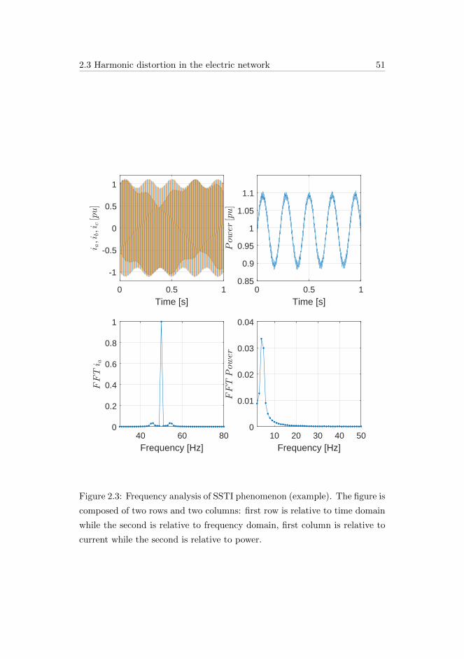
2.3 Harmonic distortion in the electric network 51
0 0.5 1
Time [s]
-1
-0.5
0
0.5
1
0 0.5 1
Time [s]
0.85
0.9
0.95
1
1.05
1.1
40 60 80
Frequency [Hz]
0
0.2
0.4
0.6
0.8
1
10 20 30 40 50
Frequency [Hz]
0
0.01
0.02
0.03
0.04
Figure 2.3: Frequency analysis of SSTI phenomenon (example). The figure is
composed of two rows and two columns: first row is relative to time domain
while the second is relative to frequency domain, first column is relative to
current while the second is relative to power.

52 Sub-Synchronous Torsional Interactions in Electrical Networks
In the following, a few additional details and remarks about figure 2.3
are listed:
• This is only a simulated example built in MATLAB®, where all the
quantities are normalised in per-unit (pu);
• the only purpose of this figure is to clarify some possible SSTI causes,
the magnitude of the oscillations has been intentionally amplified to
enhance the distortion;
• in order to achieve more realistic results the three line currents have
been noised with an AWGN (Additive White Gaussian Noise);
• the reason why the peak of power spectrum is definitely lower than 1 pu
is that the main component of the spectrum is the DC component, thus
the y-axis has been scaled in order to highlight the peak at fD.
From the previous simple example comes out that if fD is equal to the first
TNF of TG, then this particular load would excite the mechanical system
in correspondence of its resonance frequency, therefore it should be able to
activate and feed SSTI phenomenon. However, someone can note that in
a real electric network it would be a very unlucky situation to have two
perfect side-bands as the ones showed in this example, perfectly centered
in f − 1TNF and f + 1TNF . The fact is that the distortion introduced
by non-linear load leads to disturbances in a wide range of frequencies that
can include also the two side-bands, but the mechanical system is sensitive
only to these specific frequencies and does not respond to the other ones.
Therefore, it is clear that to trigger SSTI oscillations it is not strictly required
to have a spectrum of line currents exactly equal to the one showed in figure
2.3, indeed it is just enough to have a continuous disturbance that insists
within a frequency interval that contains the critical frequencies f − 1TNF
and f + 1TNF .

2.4 SSTI mitigation: damping system proposal 53
2.4 SSTI mitigation: damping system proposal
In section 2.2 the causes of Sub-Synchronous Torsional Interaction have been
explained. The oscillations in the absorbed currents ∆i lead to oscillation in
the electric torque ∆Te that finally leads to oscillations in the TG rotational
speed ∆ω. In turn, mechanical oscillations ∆ω produce oscillations ∆V and
∆i within the electrical network, thus the loop is closed.
Figure 2.4 represents a schematic of a power generation unit with a SSTI
damping system included.
GT
Gear Box
G
3~
1TNF
SSTI damping system
∆ω
ω
Electric
Network
idamp
Turbo-generator
Band-pass
filter
Figure 2.4: Schematic of SSTI mitigation system.
As shown in figure 2.4, the proposed SSTI damping system should be
inserted within the electric network, indeed the main purpose is not a me-
chanical damping of the torsional vibrations but it aims to compensate the
electric oscillations by introducing an active load. The active load is a con-
trolled load that adapts its own request of power in function of the measured
mechanical oscillations ∆ω. As described in [1] and [2], the measurement
of the angular velocity of a rotating shaft is based on a cogwheel installed
on the shaft itself. Once the angular velocity ω of the shaft is known, the
harmonic at 1TNF can be isolated by introducing a simple band-pass filter
centered in 1TNF . Therefore, the main purpose of the damping system is to
balance the fluctuations of electric power within the electric network. In this

54 Sub-Synchronous Torsional Interactions in Electrical Networks
way the power transfer at 1TNF between the electric grid and TG should
be avoided, indeed the oscillations are bounded within the electric network.
In practice, this damping system has the same function of a capacitor in an
electric circuit or an accumulator in a hydraulic circuit, indeed it alterna-
tively accumulates and releases energy in order to keep the power request as
constant as possible. The only difference is that this damping system should
behaves in this way only at 1TNF , while it should be transparent to all the
other frequencies.
The schematic of the proposed damping system and its control logic are
represented in figure 2.5.
R-L
LOAD
Three-phase
electric network
IDC
∆ω Phase shifter
Gain
Firing
angle
control
IDC,ref
Damping System
Three-phase thyristor
rectifier Bridge
VDC
-
+
IDC,meas
idamp
1TNF
ω
Band-pass
filter
Figure 2.5: Schematic of SSTI damping system.
Note that the firing angle control usually is based on a classical PID con-
troller (Proportional-Integral-Derivative controller), and it can be included
inside the three-phase thyristor rectifier bridge. Practical guidelines to de-
sign and tune a PID controller can be found in many technical manuals or
article, e.g. see [4], [48] or [98].
Some additional observations are needed to completely understand the

2.4 SSTI mitigation: damping system proposal 55
high level logical diagram in figure 2.5:
• As shown in section 2.2, the electric torque oscillations ∆Te are strictly
related to torsional oscillations ∆ω, thus ∆Te and ∆ω contain exactly
the same information. Since angular speed ω is a measurement always
available and quite accurate (see [1] and [2]), it is a reasonable choice
to use a band-pass filter to isolate ∆ω from ω, and use this information
as input of the damper logic.
• the phase shifter and the gain are needed in order to maximise the
reduction of electric torque oscillation at 1TNF . ∆ω has to be ampli-
fied and delayed in order to compensate the electric oscillations within
the network. The gain and the delay can be constant values computed
offline during design phase or they can be optimised with online calcu-
lations based on adaptive model. ∆ω needs to be properly amplified
and delayed in order to compensate the differences between the phasors
∆T e(fn) and ∆ω(fn) described in paragraph 2.2.1;
• R-L load should be characterised by a resistance as small as possible
in order to minimise the power dissipation and a very large inductance
(L ' 1÷5mH). The inductor should be able to accumulate and release
energy, exactly as a spring does in a mechanical system. In this way the
inductor should filter the fluctuations of energy with frequency nearby
1TNF, thus the mechanical trains, i.e. TGs, should not be excited in
correspondence of their first torsional resonance peak;
• the average voltage VDC produced by the three-phase thyristor rectifier
bridge can be controlled by modifying the firing angle of the thyristors.
In practice, the rectifier bridge does not directly impose the current,
but it moves the firing angle modifying the voltage VDC until the cur-
rent is equal to the desired value. The rectifier bridge is able to follow
the reference current IDC,ref only if the frequency of the reference cur-
rent is definitely lower than the network frequency. Since the objective
of this damper system is the mitigation of SSTI oscillations at 1TNF

56 Sub-Synchronous Torsional Interactions in Electrical Networks
(that usually are lower than 10Hz) and the standard electric network
frequency is 50 or 60Hz, the above condition is satisfied, therefore the
rectifier bridge should be able to follow the reference.
2.5 Simulations and results
SSTI instability has been experienced for a long time and many studies
have highlighted that this phenomenon is mainly influenced by the grid size
and configuration, the number and the localization of the electrical gen-
erators and the features of the power electronic equipment used as input
stage and/or to control the large electric loads connected to the grid (e.g.
motors, pumps, fans and heaters). Many simulations have been performed
exploiting dedicated toolbox available in MATLAB®and Simulink®; in par-
ticular the modelling and simulation of the electric grid has been performed
in PLECS®2.
Several configurations have been tested, but all of them can be sum-
marised as shown in figure 2.6, where GA and GB are two separated elec-
tric generators, ZA and ZB are the two isochronous reactances, while Zc,A,
Zc,B , ZD and ZL are the line impedances. It is worth noticing that when
two or more TG units are running in an isolated system where frequency is
not dictated by a prevalent network, isochronous/droop control is the tra-
ditional and simplest way to control each train. Only one TG train has to
be controlled in isochronous mode, thus this unit is controlled to maintain
a constant speed (due to 50 or 60Hz), regardless of the load. The value
of the active power supplied to the load can not be set and the machine
faces to all load variations; i.e., if an increase in load power demand oc-
curs, GT consequent response is a speed reduction, immediately corrected
by the speed controller increasing the gas quantity supplied to the machine.
If more TGs operate in parallel, the other units have to be controlled in
2 PLECS®is a very interesting tool for high-speed simulations of power electronics and
thermodynamics that can be easily integrated in MATLAB®and Simulink®environment.
More details can be retrieved from the PLECS user manual, available at [75].

2.5 Simulations and results 57
droop mode. In droop control mode the speed is not imposed, indeed the
power supplied to the load follows the droop load control curve, i.e. a linear
curve that describes the connection between the turbine speed variation and
the corresponding variation in the load power request. Detailed description
of isochronous/droop mode control can be retrieved in many manuals, see
e.g. [9], [99], [74] and[44] .
GA
Disturb. Load
Damper
GBDroop
Isoch
Passive Load
11/31.5 kV
11/31.5 kV
31.5/11 kV
@1TNF
PF=0.9
ZA ZC,A
ZBZL
31.5/1.2 kV
ZD
ZC,B
Figure 2.6: Schematic of electric power generation and distribution system.
Note that the SSTI oscillations are imposed by introducing a fake load
that absorbs power at 1TNF ; in this way it is simple to activate/deactivate
SSTI during the simulation.
As explained previously, different configuration of electrical grid can bring
to different risk of incurring in SSTI phenomenon; this is the reason why
several network configurations have been simulated and tested. In particular,
the set of simulations has been studied aiming to consider different line
impedances, critical events such as load steps and different torsional models
of TGs. In the following some results that provide general features of SSTI
are reported.
Figure 2.7 shows the torsional oscillations of the isochronous GT in three
different cases (normalised in pu). In figure 2.7a, the disturbing load and the
passive load are inserted at t = 0 s, indeed there is an initial undershoot due
to the electric passive load that makes the GT speed decrease. However,
in a few seconds the GT governor brings the average speed towards 1 pu.
Moreover the disturbing load at 1TNF induces larger and larger torsional
oscillations, and when the damping system is activated (t = 10 s) the oscil-

58 Sub-Synchronous Torsional Interactions in Electrical Networks
0 5 10 15 20
Time [s]
0.9985
0.999
0.9995
1
1.0005
1.001
GT
A S
peed
[pu]
(a) Damping of torsional oscillations.
0 5 10 15 20 25 30 35
Time [s]
0.997
0.998
0.999
1
1.001
GT
A S
peed
[pu]
(b) Damping of torsional oscillations with load step.
0 5 10 15 20 25 30 35
Time [s]
0.996
0.998
1
1.002
GT
A S
peed
[pu]
(c) Damping of torsional oscillations with load rejection.
Figure 2.7: Simulation results of three examples of torsional oscillations
damping.

2.5 Simulations and results 59
lation magnitude is ' 7.5 10−4 pu. When the damping system is turned on
the oscillation are reduced of ' 60% in about 5 s.
This behaviour is approximately equal to what happens in figures 2.7b
and 2.7c: besides that, these tests simulate how the system responds to a
load step (figure 2.7b) and to a load rejection (figure 2.7c), both of them at
t = 20 s. Note that load step indicates that the load gets increased, while
load rejection indicates that the load decreases. In addition to the initial
undershoot/overshoot due to load changes, it is worth noticing that when
the system gets a greater load the oscillations are reduced, while when the
system rejects a part of the load the oscillations are intensified. This is a
general rule, indeed many researchers has experienced that unloaded electric
generation plants are more sensitive to SSTI issues.
Moreover, it has been observed that in very large electric networks it
is less frequent to have SSTI; this is due to the fact that in wider electric
grids there are more dissipations, thus the disturbances at 1TNF (as all the
other disturbances) are automatically reduced. Similar reasonings can justify
also the fact that generation plants composed of several TGs in parallel
(more than 3/4 TGs) are not interested by SSTI, indeed in this case the
disturbances at 1TNF are distributed between several trains, thus each TG
does not receive enough energy at 1TNF to trigger SSTI phenomenon, and
dangerous torsional oscillations are avoided.
Figure 2.8 shows how the three-phase thyristor rectifier bridge works. As
shown in figure 2.8a each phase current (briefly indicated as idamp in figure
2.5) has several discontinuities when the relative thyristor is turned on/off.
By controlling the firing angle it is possible to make the DC link current
follow the reference current (figure 2.8b). Note that the DC link can only
absorb a positive current, and this is the reason why it is necessary to add
a constant offset to the reference current.
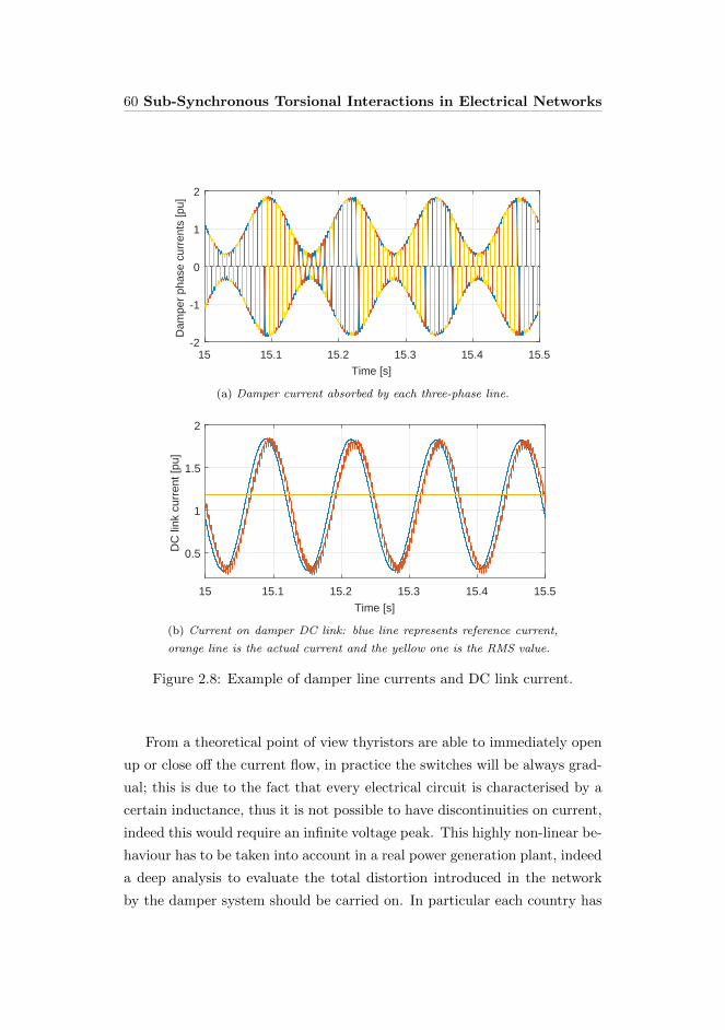
60 Sub-Synchronous Torsional Interactions in Electrical Networks
15 15.1 15.2 15.3 15.4 15.5
Time [s]
-2
-1
0
1
2D
ampe
r ph
ase
curr
ents
[pu]
(a) Damper current absorbed by each three-phase line.
15 15.1 15.2 15.3 15.4 15.5
Time [s]
0.5
1
1.5
2
DC
link
cur
rent
[pu]
(b) Current on damper DC link: blue line represents reference current,
orange line is the actual current and the yellow one is the RMS value.
Figure 2.8: Example of damper line currents and DC link current.
From a theoretical point of view thyristors are able to immediately open
up or close off the current flow, in practice the switches will be always grad-
ual; this is due to the fact that every electrical circuit is characterised by a
certain inductance, thus it is not possible to have discontinuities on current,
indeed this would require an infinite voltage peak. This highly non-linear be-
haviour has to be taken into account in a real power generation plant, indeed
a deep analysis to evaluate the total distortion introduced in the network
by the damper system should be carried on. In particular each country has

2.6 Results analysis and conclusions 61
its own regulations (grid code) about the maximum THD allowed in a grid,
thus the damper system has to be designed considering these legal limits.
The last observation is about the power that needs to be dissipated by
the damper system. If the damper were composed of an ideal inductor it
would exchange with the network only reactive power: this means that the
absorbed power would be a zero-mean power, without any real transfer of
energy. On the contrary, the real damper system is characterised by a certain
resistance: it should be as small as possible but always greater than the ideal
0Ω.
Theory of electrical engineering (see e.g. [3]) states that the power as-
sociated to a current i(t) that flows through an inductor L in series with
resistance R is equal to
PRL(t) = PL(t) + PR(t) = L · ∂i(t)∂t︸ ︷︷ ︸
VL
·i(t) +R · i(t)2. (2.8)
By consequence, the energy absorbed by the damper should be equal to
ERL(t) =
∫ t
0
(PL(t) + PR(t)) dt =1
2Li(t)2 +
∫ t
0
(R · i(t)2)dt. (2.9)
Equation (2.9) clearly states that the energy diverges in time, thus the
system sizing and above all the cooling system has to be designed in order
to be able to manage this quantity of energy. Indeed, the cooling system
is supposed to be able to dissipate enough energy in order to prevent the
damper system from overheating.
2.6 Results analysis and conclusions
As mentioned in the previous sections, SSTI phenomenon is deeply influ-
enced by several features both of mechanical and electrical systems. As
a consequence, it is quite hard to provide general rules to quantitatively
compute SSTI risk. Each particular site would require a dedicated analysis
in order to assess the risk of occurrence of this unstable phenomenon and,

62 Sub-Synchronous Torsional Interactions in Electrical Networks
if necessary, to quantify the goodness of a damping system introduced to
mitigate the oscillations.
However, simulations have highlighted some SSTI general features and
some guidelines that should be taken into consideration during design phase
in order to minimise the occurrence of this events. They can be summarised
in these points:
i. Larger electric networks (thus larger values of impedances ZC,A and
ZC,B referring to figure 2.6) are less compatible with SSTI instability.
In very wide electric grid, e.g. a prevalent network, the power of the
disturbs that can lead to SSTI is negligible with respect to the network
power capacity, and the physical sizes of the grid allow the dissipation
or the temporary storage of all the harmonics different from the stan-
dard one;
ii. ∆ω can be measured either from the isochronous GT or the droop
mode controlled GT. Sometimes it can happen that the optimal values
for the gain and the phase delay depend on the source of ∆ω. Nev-
ertheless, the proposed damper logic is effective independently from
where ∆ω is taken. This means that in an electric generation plant
composed of several TGs, the damper system can take the angular
speed measurement from any TG, without restrictions. Obviously, the
numerical calibration of the damper logic will be connected to the par-
ticular choice of the source of ∆ω;
iii. the most critical situation concerning SSTI phenomenon has been ex-
perienced when the electrical power request is very small. Once again,
this behaviour can be explained considering the relative weight of dis-
turbing load with respect to the total power request;
iv. in some simulations two different TGs (i.e. with different mechanical
size and TNFs) have been considered. The results have highlighted
that when the damping system mitigates the torsional oscillations in-
duced in one TG, the other one is not affected by the damper action.

2.6 Results analysis and conclusions 63
Since very different TNFs means that the two TGs are sensitive to
very distant frequencies, this result is reasonable; however, it is very
important to be sure that the damper system, in addition to mitigate
SSTI, does not introduce any negative effect within the system;
v. load step and load rejection events do not represent critical events by
themselves. However, as described in bullet (iii), it has to be consid-
ered that SSTI criticality changes with the total power request, thus
during load rejection events the system moves towards a configuration
characterised by a major SSTI risk.

64 Sub-Synchronous Torsional Interactions in Electrical Networks

Chapter 3
Gas Turbine Modelling and
Model-Based Estimation
Many different types of GTs have been developed in the past years
and they can be broadly classified as single-shaft GT, mainly
generator drive application, or two-shaft GT, mainly mechanical
drive application. In this chapter the characterisation and the
modelling of a particular two-shaft GT will be addressed; first
of all a static a-priori model has been proposed and it has been
trained with a massive dataset, then all the measurements and
equations have been merged within a Kalman filter. Finally, the
quality of the model has been evaluated also by exploiting field
data and conclusions have been drawn.
3.1 Gas turbine general description
The first operating gas turbine was proposed in the beginning of twentieth
century and it had a very low thermal efficiency. In a few decades the gas
turbines technology has been deeply enhanced and they have been introduced
in a wide range of practical and industrial applications, such as:
• electric power generation: a gas turbine is directly connected to an
65

66 Gas Turbine Modelling and Model-Based Estimation
electric generator running at constant speed. The speed depends on
the number of magnetic poles of the generator and the standard elec-
tric grid frequency, that can be 50 or 60Hz. Sometimes a gearbox is
required to scale the GT speed to the generator speed;
• compressor drive application: in this case GT can be designed in order
to have the same rotational speed of the compressor, thus gearbox
is not always strictly required. Compressor rotating speed is usually
asked to vary within a certain operating range, thus the GT that drives
the compressor has to be designed in order to be able to adapt its own
rotational speed;
• aircraft propulsion: the basic development in this field took place for
high-speed military aircrafts. In this case the engine is asked only to
produce enough power to drive the compressor, then the gas leaving the
turbine at high pressure and temperature is expanded to atmospheric
pressure in a propelling nozzle to produce a high velocity jet. Only in
the early 1950s GTs started to be used in civil aircraft applications;
• marine and land transportation: GTs have been used as prime mover
for ships, trains and trucks1. Usually GTs for these applications are
derived from aircraft engines and for this reason they are often referred
to as aero-derivative GTs. Aero-derivative GTs are generally lighter
weight, physically smaller and have a better partial load performance
with respect to industrial GTs (which are usually referred to as heavy-
duty GTs), but they are characterised by more frequent maintenance
intervals.
When GTs are required to operate at a fixed speed and fixed load the single-
shaft configuration is the most suitable (figure 3.1), indeed the engine has
not to be flexible and ready to changes of rotational speed.
1Due to several technical reasons, GTs did not provide a significant contribution to
land transportation; current proposals would use GTs to generate electricity with separate
electric motors on the driving wheels.

3.1 Gas turbine general description 67
Axial
Compressor
Combustion
chamber
Fuel
Power Turbine
Load
Figure 3.1: Single-shaft GT schematic.
On the contrary, when flexibility in operation is of great importance, e.g.
when driving a variable speed load such as a centrifugal compressor, the use
of a mechanically free power turbine is appreciable. In this two-shaft config-
uration (figure 3.2) the High-Pressure Turbine (HPT) drives the compressor
and the combination acts as a Gas Generator (GG) for the Low-Pressure
Turbine (LPT). LPT is the free power turbine which is aerodynamically but
not mechanically coupled to HPT. Aircraft engine may be used as gas gen-
erator for driving an electric generator or a mechanical load, indeed it is just
enough to make exhaust gas expand through a power turbine such as LPT
rather than the original exhaust nozzle.
Axial
Compressor
Combustion
chamber
Fuel
High Pressure
Turbine
Load
Low Pressure
Turbine
Gas Generator
Figure 3.2: Two-shaft GT with separated power turbine schematic.

68 Gas Turbine Modelling and Model-Based Estimation
Figures 3.3 shows an example of two-shaft GT that has been heavily
installed worldwide both in mechanical drive and power generation applica-
tions.
Figure 3.3: GE LM2500+G4, a two-shaft aero-derivative GT. This GT be-
longs to GE LM series, where LM states for Land & Marine. Courtesy of
BHGE (source www.bhge.com).
On the other hand, figure 3.4 shows an example of single-shaft GT,
mainly used in power generation plants.

3.1 Gas turbine general description 69
(a) Single-shaft gas tubine, first view.
(b) Single-shaft gas tubine, second view.
Figure 3.4: Two different views of a single-shaft GT. Courtesy of BHGE
(source www.ge.com).

70 Gas Turbine Modelling and Model-Based Estimation
3.1.1 GE LM2500 overview
The LM2500 gas turbines are simple cycle, two-shaft, high-performance en-
gines. They derived from GE TF39 and CF6− 6 aircraft engines, and they
consist of a gas generator and a power turbine. These gas turbines are single
rotor GTs which are aerodynamically coupled with a power turbine. Power
turbine operates at a nominal speed of 3600 rpm, making it ideal for 60Hz
electric generation service. Alternatively, it can also operate efficiently over
a cubic load curve for mechanical drive applications.
Depending on the model, AC is composed of 16 or 17 stages, while the
power turbine can have 2 or 6 stages. AC does not have Inlet Guide Vane
(IGV), but it has the Variable Stator Vane (VSV), i.e. a particular system
that modifies the geometry of the first AC stages in order to allow it to
properly work at any load and speed. LM2500 GTs are usually suitable for
two types of power turbines:
1. a six-stage low speed power turbine, with a nominal speed of 3600 rpm;
2. a two-stage high speed power turbine, with a nominal speed of 6100 rpm
(this power turbine is usually preferred in mechanical drive applica-
tions).
Typical power of these GTs is between 25MW and 33MW .
There are three GTs that belongs to LM2500 family, whose peculiarities
are summarised in table 3.1:
i. LM2500 (see [29]);
ii. LM2500+ (see [30]);
iii. LM2500+G4 (see [31]).

3.1 Gas turbine general description 71
LM2500 LM2500+ LM2500+G4
Max power [kW ] 25060 30200 35320
Fuel cons.[
gkW ·h
]227 215 214
Heat rate[
kJkW ·h
]9705 9227 9150
Exhaust gas flow [kg/s] 70.5 85.9 93
Exhaust gas temp. [K] 839 791 822
Turbine speed [rpm] 3600 3600 3600
Thermal efficiency [ ] 36 % 38 % 39 %
Weight [kg] 4700 5250 5250
Table 3.1: LM2500 GT family characteristics.
Moreover, depending on combustion chamber type, LM2500 GTs can be
classified as Singular Annular Chamber (SAC), where there are not limita-
tions on NOx emissions, or Dry Low Emission (DLE), where NOx emissions
are limited to 25 ppm.
This thesis work will focus on a particular two-shaft aero-derivative GT
which belongs to LM2500 family, i.e. LM2500+G4 DLE.

72 Gas Turbine Modelling and Model-Based Estimation
3.2 GE LM2500+G4 DLE detailed modelling
based on NPSS
Figure 3.5 depicts in a qualitative temperature-entropy diagram the differ-
ence between the ideal and the real thermodynamic cycle of a single-shaft
GT. This thermodynamic cycle is the well-known Brayton cycle. The real
cycle tends to move away from the ideal one because of many non-idealities
such as dissipations, frictions, not ideal combustion, engine ageing or degra-
dation, mechanical losses and so on.
T
S
1
2is2real
3is 3real
4is
4real
Figure 3.5: Schematic representation of ideal/real Brayton cycle of a single-
shaft GT.
Since every GT model has its own peculiarities, in the past decades many
efforts have been made to develop computational methods for the definition
and the resolution of the very complex non-linear differential equations that
aerodynamically, mechanically and thermodynamically describe the GT en-
gine. National Aeronautics and Space Administration (NASA) has intro-
duced the so-called Numerical Propulsion System Simulation (NPSS), i.e.
an object-oriented, multi-physics, engineering design and simulation envi-
ronment. There are many detailed technical reports about NPSS, see e.g.

3.2 GE LM2500+G4 DLE detailed modelling based on NPSS 73
[62], [49] and [20]. NPSS is a full engine multidisciplinary simulation tool
developed for aerospace industry but also used in oil and gas power industry,
indeed it provides an environment for the analysis and the design of aircraft
propulsion systems, rocket cycles and many other thermodynamic processes.
Actually, NPSS implements and solves all the differential equations that de-
scribe in a detailed and rigorous way the system; for this reason, in this work
NPSS model will be considered as reference.
NPSS is currently managed by a consortium including research institutes
and industrial members. Different licensing scheme are available both for
academic and commercial use. The NPSS software exploited in this work has
been made available by Nuovo Pignone - Baker Hughes, a GE Company and
it provides expected values about the GE LM2500+G4 DLE main physical
quantities.
In order to adapt the average engine model to real conditions it contains
six corrective parameters (CPs) useful to modify the thermodynamic and
flow efficiency respectively of AC, HPT and LPT. Four CPs are relative to
thermodynamic and flow efficiency of AC and HPT, while the other two CPs
are relative to thermodynamic and flow efficiency of LPT. In the next sec-
tions some mathematical models regarding each section of GE LM2500+G4
DLE (presented in paragraph 3.1.1) will be introduced: these models have
been both tuned and validated using NPSS model as a reference. In par-
ticular, the datasets used to tune/validate mathematical models are listed
below:
i. nominal NPSS dataset : this dataset has been obtained using NPSS by
exploring all the feasible operating conditions (different fuel compo-
sitions, delivered power and inlet conditions), always maintaining the
six CPs equal to 1. This dataset has been used during validation phase
in order to figure out the nominal behaviour of the machine;
ii. GG extended NPSS dataset : this dataset has been obtained using
NPSS by exploring all the GG feasible operating conditions; each sin-
gle CP relative to GG has been moved from 0.98 to 1.02 with step

74 Gas Turbine Modelling and Model-Based Estimation
of 0.01 (i.e., each operating condition has been simulated in 54 = 625
different configurations of CPs). On the contrary the two CPs relative
to LPT have always been kept equal to 1, in turn this dataset ranges
within all the possible configurations of the gas generator maintaining
the nominal model concerning the LPT. This dataset has been used
to validate the proposed models in all the possible configurations of
the GG. The reason why this dataset is significant is that the GG of
this gas turbine can be coupled with different type of LPT, thus it
would be very useful to validate the proposed model with respect to
GG variations and then introduce the LPT as an additive model.
iii. full extended NPSS dataset : this dataset has been obtained using NPSS
by exploring all the feasible operating conditions, and moving each
single CP from 0.98 to 1.02 with step of 0.01. This means that each
operating condition has been simulated in 56 = 15625 different config-
urations of CPs. This massive dataset has been used to validate the
proposed models in all the possible configurations. Figures 3.6 and
3.7, referring to the nomenclature reported in table 3.2, show the per-
centage variations introduced by CPs changes on each quantity with
respect to nominal NPSS dataset. It is worth noticing that GG ex-
tended NPSS dataset is a subset of full extended NPSS dataset, indeed
the former is completely included within the latter;
iv. real trend dataset : some datasets taken from existing LM2500+G4
DLE running sites have been used to validate the proposed models.
Obviously these datasets are very important because they allow the
validation with respect to real data; however these trends contains
only quantity that can be measured by available sensors, thus it is not
trivial to use these datasets to validate the model.

3.2 GE LM2500+G4 DLE detailed modelling based on NPSS 75
-3 -2 -1 0 1 2 3
TACout dev [%]
0
0.005
0.01
0.015
0.02
Rel
ativ
e F
requ
ency
(a) T outAC percentage deviation.
-4 -3 -2 -1 0 1 2 3 4
THPTin dev [%]
0
0.02
0.04
0.06
0.08
Rel
ativ
e F
requ
ency
(b) T inHPT percentage deviation.
-5 0 5
THPTout dev [%]
0
0.01
0.02
0.03
0.04
Rel
ativ
e F
requ
ency
(c) T outHPT percentage deviation.
Figure 3.6: NPSS temperatures percentage deviation: full extended NPSS
dataset versus nominal NPSS dataset.
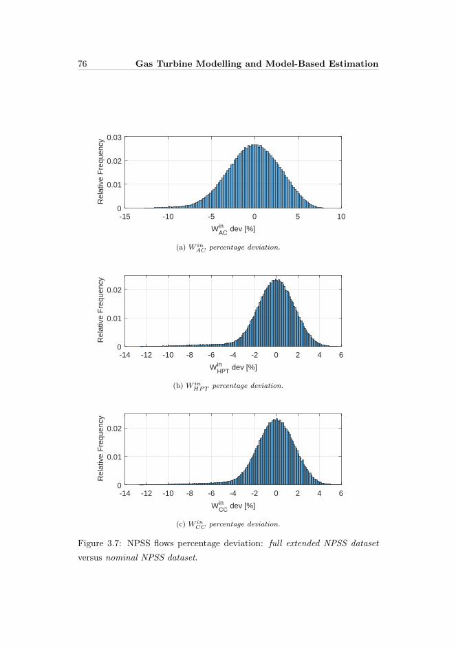
76 Gas Turbine Modelling and Model-Based Estimation
-15 -10 -5 0 5 10
WACin dev [%]
0
0.01
0.02
0.03
Rel
ativ
e F
requ
ency
(a) W inAC percentage deviation.
-14 -12 -10 -8 -6 -4 -2 0 2 4 6
WHPTin dev [%]
0
0.01
0.02
Rel
ativ
e F
requ
ency
(b) W inHPT percentage deviation.
-14 -12 -10 -8 -6 -4 -2 0 2 4 6
WCCin dev [%]
0
0.01
0.02
Rel
ativ
e F
requ
ency
(c) W inCC percentage deviation.
Figure 3.7: NPSS flows percentage deviation: full extended NPSS dataset
versus nominal NPSS dataset.

3.3 A-priori static model of GE LM2500+G4 DLE 77
3.3 A-priori static model of GE LM2500+G4
DLE
In parallel with the technical improvement of GTs, many researchers have
understood the importance of developing a mathematical model able to de-
scribe how the system acts in each operating point. Such a model could
be very useful to estimate quantities that can not be directly measured by
transducers, to provide validation and redundancy of quantities measured
by physical sensors, or to enhance control law that could be based not only
on the direct measurements but also on the knowledge of the plant inter-
nal model that describes from a mathematical point of view the physical
laws on which the system is based on. GTs operating principles and theory
has been widely studied and many handbooks and technical manuals about
this topic have been written (see e.g. [24], [19], [72], [16], [73], [87] and
[32]). Besides, in literature there are many examples of GTs models based
on thermodynamic relationships, both for aero-derivative and heavy duty
GTs (see e.g. [40], [106], [53] and [23]). A common issue in GTs modelling,
as shown in [108], is that the system is very complex and highly non-linear,
thus it is difficult to develop a general method with validity extended to all
the possible operating conditions. For instance, in [55] at first a GT model
is implemented in MATLAB®and Simulink®, then the model is tested and
validated in many different operating and environmental conditions. In the
last years GT control and identification through neural networks has been
proposed (e.g. [107] and [54]). Also GT MPC (Model Predictive Control),
although it is not widely used in industrial applications, has been addressed
by many researchers (see e.g. [80], [17] and [50]).
In this chapter an a-priori static model of the GE LM2500+G4 DLE will
be introduced. Details of this particular aero-derivative GT are described
in paragraph 3.1.1, while figure 3.3 is a picture of this GT. Referring to the
nomenclature reported in table 3.2, and considering the usually available
measurements in typical oil and gas applications, the inputs and outputs
lists for the overall static model are:

78 Gas Turbine Modelling and Model-Based Estimation
• Inputs: T inAC , pinAC , T outAC , poutAC , LHV , Tfuel, cp,fuel, ToutHPT , poutHPT ;
• Outputs: W inAC , T outAC , W in
CC , pinHPT , T inHPT , W inHPT .
Note that, concerning the static model, T inAC can be considered both as input
and output at the same time. This is due to the fact that in correspondence of
the last AC section thermocouples are always inserted to directly measure the
AC discharge temperature, but this quantity can also be estimated regardless
its measurement by the static model that will be introduced in paragraph
3.3.1. Furthermore, as will be explained in the next paragraphs, flows can
be estimated in two different ways. This features about T inAC and the flows
through the GT will be exploited to improve the estimation accuracy and to
enhance the model performance.
Symbol Unit Definition
pinAC [kPa] AC inlet pressure
T inAC [K] AC inlet temperature
poutAC [kPa] AC outlet pressure
T outAC [K] AC outlet temperature
W inAC [kg · s−1] AC inlet airflow
Wbleed [kg · s−1] Bleed airflow
W inCC [kg · s−1] Combustion chamber inlet airflow
Wfuel [kg · s−1] Total fuel flow
W inHPT [kg · s−1] HPT inlet airflow
W outHPT [kg · s−1] HPT outlet airflow
cp, cv [J · (K · kg)−1] Isobaric/Isochor heat capacity
γ [ ] Isobaric/Isochor heat capacity ratio
T inHPT [K] First HPT section temperature
pinHPT [kPa] First HPT section pressure

3.3 A-priori static model of GE LM2500+G4 DLE 79
T outHPT [K] Last HPT section temperature
poutHPT [kPa] Last HPT section pressure
LHV [kJ · kg−1] Fuel lower heating value
NHPT [rpm] HPT rotational speed
NLPT [rpm] LPT rotational speed
ηisAC [ ] Isentropic AC efficiency
ηisHPT [ ] Isentropic HPT efficiency
ηCC [ ] Combustion efficiency
Tfuel [K] Fuel temperature
JGG [kg ·m2] GG inertia
Table 3.2: GE LM2500+G4 DLE main quantities nomenclature
3.3.1 Axial compressor model
The first mathematical model able to describe the behaviour of an axial
compressor was introduced by Moore and Greitzer (see [66] and [67]). In
the past decades many researchers have enhanced this model (see e.g. [13],
[95], [63] [34]); this is a very complete model and it allows the simulation
of AC behaviour even when it operates near instability regions (i.e. stall,
surge or choking). However, Moore-Greitzer model requires an accurate
identification of many machine-dependent parameters, thus it is particularly
linked to the specific compressor under analysis. In this work an alternative
model is used, indeed AC modelling is split in two separated modules: the
first one provides a calculation of the flow through the inlet stage of the AC,
while the second addresses the AC discharge temperature calculation.
Table 3.3 shows the inputs and the outputs of the proposed AC a-priori
static model.

80 Gas Turbine Modelling and Model-Based Estimation
Inputs Outputs
T inAC W inAC
pinAC T outAC
poutAC
Table 3.3: Inputs and outputs of the proposed AC model.
Axial compressor inlet airflow
The Law of the Ellipse, which is usually referred to as Stodola’s Law, provides
a simple method for calculating the airflow through a multi-stage AC (more
details can be retrieved in [39] and [37]). Obviously this is a highly non-linear
phenomenon and it can describe the AC behaviour only within nominal
operating range, thus it is not suitable to model the AC flow when stall,
surge or choking occur. Equation (3.1) is an approximation of the Law of
the Ellipse which can be exploited to compute AC inlet flow
W inAC = cAC ·
pinAC√T inAC
·
√1−
(pinACpoutAC
)2
, (3.1)
where cAC is a variable coefficient that assumes different values in different
operating conditions. Several NPSS simulations have been performed to
find out a map that describes how it changes when the inlet AC conditions
and the GG speed change. In particular nominal NPSS dataset has been
exploited, and it has underlined that inlet pressure pinAC does not affect too
much this coefficient, thus the map showed in figure 3.8 is a family of curves
that describes how cAC changes in function of T inAC and NHPT .
Note that one of the reason why coefficient CAC is not constant is that
the AC under analysis can change its geometry thanks to VSV (Variable
Stator Vanes), whose angle is scheduled in function of NHPT , pinAC and T inAC .
Since VSV are controlled in open-loop mode and their position depends only
on NHPT , pinAC and T inAC , it is possible to include their effects on the global
system inside the static model; in this way, VSV modelling is not required,

3.3 A-priori static model of GE LM2500+G4 DLE 81
260 270 280 290 300 310
100
150
200
NHPT
Figure 3.8: AC flow coefficient map.
indeed it is automatically considered by CAC map.
Axial compressor discharge temperature
Air temperature obviously increases between AC suction and discharge.
Considering an ideal isentropic compression, the relation between suction
and discharge thermodynamic properties is given by equation (3.2).
T outAC,is
T inAC,is=
(poutAC
pinAC
) γair−1
γair
(3.2)
where γair is defined as the isobaric and isochor heat capacity ratio relative to
air (thus it is known and almost constant) and the subscript “is” states that
the quantity is referred to an ideal isentropic transformation. The previous
equation can be generalised introducing the isentropic efficiency ηAC,is. As
shown in figure 3.5, the temperature at the end of AC in real cycle is greater
than the temperature at the same section in the ideal cycle. In turn, it is
possible to define the isentropic AC efficiency ηAC,is as
ηAC,is =T outAC,is − T inACT outAC − T inAC
. (3.3)

82 Gas Turbine Modelling and Model-Based Estimation
By merging and manipulating equations (3.2) and (3.3), it is immediate to
obtain
T outAC
T inAC= 1 +
1
ηAC,is
[(poutAC
pinAC
) γair−1
γair
− 1
]. (3.4)
Starting from known inlet conditions, equation (3.4) describes the rela-
tionship between temperature and pressure at AC discharge. This means
that poutAC and T outAC are strictly connected, thus it is sufficient to measure
only one of them to compute the other one.
Isentropic efficiency ηAC,is is not constant. Even without considering
efficiency degradation due to ageing, it is necessary to know how it changes in
different operating conditions. Once again, nominal NPSS dataset has been
exploited in order to find out a map that describes how it varies with T inAC
and NHPT . As seen for cAC , inlet pressure does not affect this coefficient,
thus the map can be simplified (figure 3.9).
Note that this map takes as input the corrected axial compressor airflow
W inAC,c, defined as
W inAC,c = W in
AC ·
√T inAC,nomT inAC
· pinACpinAC,nom
,
where T inAC,nom and pinAC,nom are the ambient nominal value of temperature
and pressure, respectively equal to 288.15K and 1013 kPa. Corrected air-
flow is a very useful normalisation that allows to consider all the possible
combinations of flow, temperature and pressure in a single quantity.
3.3.2 Combustion chamber model
In literature there are many examples of combustion models that were intro-
duced to describe the gas-dynamics and the combustion process of particular
GTs (see e.g. [7], [101] and [82]). Other models, such as the ones proposed
in [64], [18], [100] and [8], are aimed to control combustion instabilities (e.g.
acoustic pressure oscillations) and harmful emissions (mainly NOx and CO
emissions). These models are very specific and they have been introduced

3.3 A-priori static model of GE LM2500+G4 DLE 83
70 75 80 85 90 95 100 105 1100.82
0.84
0.86
0.88
0.9N
HPT
Figure 3.9: AC isentropic efficiency map.
to face certain well defined issues connected to combustion; the objective
of this work is to achieve a global energetic characterisation of the combus-
tion chamber, thus it is not required a detailed model able to describe the
thermodynamic and aerodynamic behaviour of the whole system.
Table 3.4 shows the inputs and the outputs of the combustion chamber
model considered in this work. Fuel isobaric heat capacity needs to be known
in order to produce an energy balance based on real fuel chemical properties.
Unlike what happens in AC, the flow through the combustion chamber is not
composed only by air, indeed it is a mixture; as shown in [14], isobaric heat
capacity of a mixture is equal to a linear combination of the single isobaric
heat capacities, weighted by the mole fractions of each gas.
Combustion chamber airflow
In the particular aero-derivative gas turbine under analysis, before entering
the combustion chamber there is a bleed valve that is used as actuator to
control the GT. Thanks to this valve it is possible to avoid GT unstable
behaviour, indeed it can move the AC operating point away from surge
region of the characteristic compressor map (see e.g. figure 1.4). Clearly
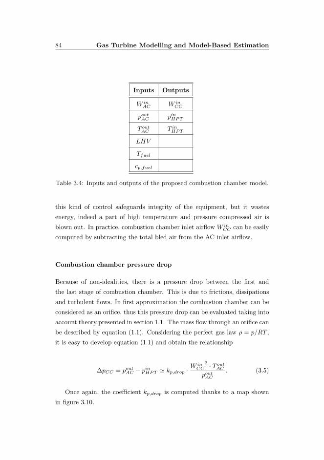
84 Gas Turbine Modelling and Model-Based Estimation
Inputs Outputs
W inAC W in
CC
poutAC pinHPT
T outAC T inHPT
LHV
Tfuel
cp,fuel
Table 3.4: Inputs and outputs of the proposed combustion chamber model.
this kind of control safeguards integrity of the equipment, but it wastes
energy, indeed a part of high temperature and pressure compressed air is
blown out. In practice, combustion chamber inlet airflow W inCC can be easily
computed by subtracting the total bled air from the AC inlet airflow.
Combustion chamber pressure drop
Because of non-idealities, there is a pressure drop between the first and
the last stage of combustion chamber. This is due to frictions, dissipations
and turbulent flows. In first approximation the combustion chamber can be
considered as an orifice, thus this pressure drop can be evaluated taking into
account theory presented in section 1.1. The mass flow through an orifice can
be described by equation (1.1). Considering the perfect gas law ρ = p/RT ,
it is easy to develop equation (1.1) and obtain the relationship
∆pCC = poutAC − pinHPT ' kp,drop ·W inCC
2 · T outAC
poutAC
. (3.5)
Once again, the coefficient kp,drop is computed thanks to a map shown
in figure 3.10.

3.3 A-priori static model of GE LM2500+G4 DLE 85
75 80 85 90 95 100 105 110
WCCin [%]
4
4.5
5
10-4
Figure 3.10: kp,drop map.
Combustion efficiency
From a thermodynamic point of view what happens during the combus-
tion can be seen as an energy exchange between the fuel and the total flow
through the combustion chamber. The chemical energy stored in the fuel
is totally described by LHV (Lower Heating Value), which expresses the
energy released by the unit mass of fuel after a complete combustion. In
turn, ideal power introduced in the system thanks to the fuel is equal to
Pideal = LHV ·Wfuel. (3.6)
The previous equation holds the true only in the ideal case. Real power
transferred from fuel to the system is lower than Pideal, and this is mainly
due to turbulence, frictions and mixing. This phenomenon can be described
introducing the combustion efficiency ηCC
Preal = ηCC · LHV ·Wfuel. (3.7)
This efficiency is characterised by a map similar to the one showed in
figure 3.9. Considering the air and fuel isobaric specific heat capacity (re-
spectively cp,air and cp,fuel), the power balance can be expressed as follows

86 Gas Turbine Modelling and Model-Based Estimation
ηCC · LHV ·Wfuel = W inCC · (T inHPT − T outAC ) · cp,air+
+Wfuel · (T inHPT − Tfuel) · cp,fuel(3.8)
Equation (3.8) considers air and fuel as two separated systems that gain
energy. By manipulating equation (3.8) it is immediate to find out a rela-
tionship to calculate the temperature T inHPT
T inHPT =LHV · ηCC + Tfuel · cp,fuel + T outAC ·AFR · cp,air
cp,air ·AFR+ cp,fuel, (3.9)
where AFR (Air-to-Fuel Ratio) is defined as
AFR =W inCC
Wfuel.
Note that introducing the assumption T outAC = Tfuel equation (3.9) can
be drastically simplified
T inHPT = T outAC +LHV · ηCC
cp,gas · [1 +AFR]. (3.10)
Where cp,gas, as showed in [14], is the weighted sum of cp,air and cp,fuel
cp,gas =Wfuel · cp,fuel +W in
CC · cp,airWfuel +W in
CC
.
The assumption T outAC = Tfuel is unrealistic, however equations (3.9) and
(3.10) usually return very similar values: this is due to the fact that W inCC
Wfuel, thus the relative weight of Tfuel is negligible with respect to the
relative weight of T outAC .
3.3.3 High Pressure Turbine model
From a thermodynamic point of view AC and HPT are very similar: the
former compresses air, the latter expands combusted gases. Thus, it is rea-
sonable to compute HPT inlet airflow by introducing an equation very similar
to (3.1)
W inHPT = cHPT ·
pinHPT√T inHPT
·
√1−
(poutHPT
pinHPT
)2
. (3.11)

3.3 A-priori static model of GE LM2500+G4 DLE 87
As done for AC, even concerning HPT it is possible to define an isentropic
efficiency
ηHPT,is =T inHPT − T outHPT
T inHPT − T outHPT,is
. (3.12)
Equation (3.2) can be written also regarding HPT
T outHPT,is
T inHPT,is=
(poutHPT
pinHPT
) γgas−1
γgas
. (3.13)
Merging equations (3.12) and (3.13) it comes out
T outHPT
T inHPT= 1− ηHPT,is
[1−
(poutHPT
pinHPT
) γgas−1
γgas
]. (3.14)
Inputs and outputs of a-priori static HPT model are summarised in table
3.5.
Inputs Outputs
T outHPT W inHPT
pinHPT T inHPT
poutHPT
γgas
Table 3.5: Inputs and outputs of the proposed HPT model.
It is important notice that equations (3.14) and (3.9) are two indepen-
dent methods to calculate T inHPT : in order to discern between these two
calculations, T inHPT computed exploiting equation (3.14) will be referred to
as backward, while the one derived from equation (3.9) as forward.

88 Gas Turbine Modelling and Model-Based Estimation
3.4 GE LM2500+G4 DLE: Kalman Filter-based
model
Simulations have shown that the a-priori static model introduced in section
3.3 is able to match and reproduce the nominal NPSS dataset (i.e. NPSS
dataset relative to CPs equal to 1). This is not a surprising result, indeed
this model has been tuned exploiting nominal NPSS dataset. On the other
hand, for the same reason, a-priori static model leads to significant errors
with GG extended NPSS dataset and full extended NPSS dataset, and above
all with real trend dataset, where non-idealities of real plants prevent it from
providing correct estimations of GT quantities. By definition, a-priori static
model can not adapt itself to match a dataset that does not fit nominal NPSS
expected calculations. By way of example, figure 3.11 shows the percentage
error of the a-priori static estimation of T inHPT with respect to full extended
NPSS dataset.
-3 -2.5 -2 -1.5 -1 -0.5 0 0.5
THPTin est err. [%]
0
0.005
0.01
0.015
Figure 3.11: A-priori static T inHPT percentage estimation error with respect
to full extended NPSS dataset.
Comparing figure 3.11 and 3.6b it is clear that the error of the a-priori
static estimation is much greater than the variability introduced by the CPs,
thus the a-priori static model is not suitable to estimate the quantity of a
system that is different from the nominal one.
Even if this first a-priori static model is not suitable as online GT estima-

3.4 GE LM2500+G4 DLE: Kalman Filter-based model 89
tion system, it is a good starting point to develop a more general GT model,
capable of catching potential deviation of the real system with respect to
the nominal one. A-priori static GT model is strongly based on physical re-
lationships, thus it is just necessary to correct the first estimations provided
by this model trying to move the mathematical model towards real data.
Kalman Filter (KF), introduced in 1960 by Rudolf Kalman [51], is a
powerful mathematical approach to target this purpose. A complete intro-
duction to KF theory is available in appendix C. KF weights measurements
equations with dynamic model equations and it continuously provides up-
dated state variables estimations. The performance of KF strongly depends
on the quality of the model, and optimality is achieved when the actual mea-
surement process (calibration error aside) behaves as a linear system subject
to white Gaussian noise. In practice, estimations optimality is guaranteed
under very restrictive conditions. These assumptions, which are reasonable
in many applications, may turn out naive when dealing with very complex
system as GTs actually are.
In literature, many other works apply KF to similar turbomachinery
applications, even if they do not address exactly the same problem. For the
time being, KFs have been widely used in the turbine engine community for
health monitoring purpose, i.e. for fault detection and identification, false
alarms and isolation (see e.g. [47], [77], [26], [15]). In this framework, KF
is implemented to solve a different issue, i.e. the estimate of all the GT
quantities, even the ones that usually can not be directly measured.
Since GTs are highly non-linear systems, in order to turn around this
limitation it is necessary to use an Extended Kalman Filter (EKF), i.e. an
extension of classical KF oriented to non-linear systems. Non-linearities can
be located in the process model or in the measurement equations, EKF in
practice applies a classic KF to an approximated model obtained by local
linearisation of non-linear global model.
Obviously the final results are strictly dependent on the numerical choices
relative to covariance matrices P 0, Q and R, defined as follows (deeper ex-
planations about these matrices and their mathematical and physical mean-

90 Gas Turbine Modelling and Model-Based Estimation
ing can be found in appendix C):
• P 0 is the covariance matrix of initial state variables estimation;
• Q is the covariance matrix relative to process equations;
• R is the covariance matrix relative to measurement equations.
Figure 3.12 represents a high level scheme of the KF based GT model
that will be analysed in-depth in the next paragraphs.
Static
est
A-priori
static Model
+
Input
− + KF est
Kalman
Filter Combustion
chamber
model
HPT model
𝑘න ሺ∙ሻ𝑑𝜏𝑡
0
−
𝑘න ሺ∙ሻ𝑑𝜏𝑡
0
𝜗𝐴𝐶𝑊
𝜗𝐴𝐶𝑒𝑓𝑓
AC model
Figure 3.12: Schematic of GT estimation based on Kalman Filter.
Note that the proposed model is a discrete-time model with scan time
Ts, where KF is fed both with measurements inputs and static estimations
provided by a-priori static model, while KF final estimations are used to-
gether with measurements inputs to feed the subsequent static estimation

3.4 GE LM2500+G4 DLE: Kalman Filter-based model 91
step. Clearly the lower is Ts the more accurate will be the final KF estima-
tions; however, considering the very high mechanical and thermal inertias of
the studied GT, it is not strictly required to have a Ts as small as possible.
This configuration creates a closed-loop arrangement, where the outputs of
each block are inputs of the other one and vice versa.
Moreover, a-priori static model represented in figure 3.12 is slightly dif-
ferent from the one described in section 3.3, indeed AC model takes as input
two additional inputs ϑWAC and ϑeffAC . These variables are used to make the
AC static model adaptive; as a matter of fact they modify and generalise
equations (3.1) and (3.4) in this way
W inAC = cAC · ϑWAC ·
pinAC√T inAC
·
√1−
(pinACpoutAC
)2
; (3.15)
T outAC
T inAC= 1 +
1
ηAC,is · ϑeffAC
[(poutAC
pinAC
) γair−1
γair
− 1
]. (3.16)
These variables allow the static model to adapt itself to observed real
system. These additional coefficients can be computed since T outAC and W inAC
can be calculated in two independent ways.
• T outAC is estimated by a-priori static model and it is also directly mea-
sured by thermocouples;
• W inAC is estimated by a-priori static model exploiting Stodola’s Law, but
it is also involved in the flow conservation law (air is bled in many dif-
ferent sections, these airflows are computed thanks to dedicated maps).
The errors between the two values respectively of T outAC and W inAC are the
inputs of two integrators that are used to compute the numerical value of
ϑWAC and ϑeffAC . These are very simple PID controllers (Proportional-Integral-
Derivative controllers), where the proportional and the derivative gains are
set equal to 0. Thanks to these two loops it is possible to adjust the values
of ϑWAC and ϑeffAC until the outputs of equations (3.15) and (3.16) are equal
respectively to the value of flow computed with the flow balance and the
value of temperature measured by dedicated sensors.

92 Gas Turbine Modelling and Model-Based Estimation
Note that in figure 3.12 the two integrators are represented as continuous-
time integrators; actually this is only a qualitative diagram of the proposed
method, in practice discrete-time integrators have been implemented.
3.4.1 Kalman filter definition
Kalman filter can be implemented in many different ways. In particular to
define the whole KF structure it is necessary to choose suitable state vari-
ables and to specify a proper dynamic model and a complete measurement
equations set.
Although several KF structures have been tested and evaluated during
this thesis work, in this chapter only the most effective and accurate version
will be presented.
Kalman filter state variables
KF state variables vector xk is composed of the variables that have to be
estimated step after step by exploiting both the knowledge of the process
equations that describe how the system evolves and the measurement equa-
tions.
In this particular case KF state is composed of 8 variables:
i. NHPT,k - HPT rotational speed;
ii. αHPT,k - HPT rotational acceleration;
iii. T inAC,k - AC inlet temperature;
iv. T outAC,k - AC outlet temperature;
v. T inHPT,k - HPT inlet temperature;
vi. T outHPT,k - HPT outlet temperature;
vii. ϑWHPT,k - HPT flow efficiency;
viii. ϑeffHPT,k - HPT thermodynamic efficiency.
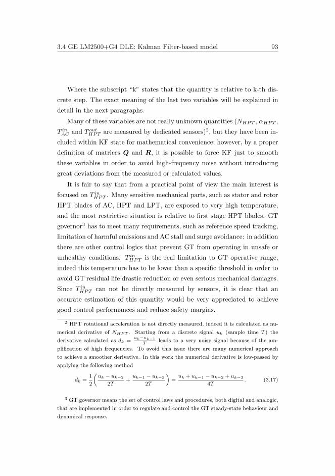
3.4 GE LM2500+G4 DLE: Kalman Filter-based model 93
Where the subscript “k” states that the quantity is relative to k-th dis-
crete step. The exact meaning of the last two variables will be explained in
detail in the next paragraphs.
Many of these variables are not really unknown quantities (NHPT , αHPT ,
T inAC and T outHPT are measured by dedicated sensors)2, but they have been in-
cluded within KF state for mathematical convenience; however, by a proper
definition of matrices Q and R, it is possible to force KF just to smooth
these variables in order to avoid high-frequency noise without introducing
great deviations from the measured or calculated values.
It is fair to say that from a practical point of view the main interest is
focused on T inHPT . Many sensitive mechanical parts, such as stator and rotor
HPT blades of AC, HPT and LPT, are exposed to very high temperature,
and the most restrictive situation is relative to first stage HPT blades. GT
governor3 has to meet many requirements, such as reference speed tracking,
limitation of harmful emissions and AC stall and surge avoidance: in addition
there are other control logics that prevent GT from operating in unsafe or
unhealthy conditions. T inHPT is the real limitation to GT operative range,
indeed this temperature has to be lower than a specific threshold in order to
avoid GT residual life drastic reduction or even serious mechanical damages.
Since T inHPT can not be directly measured by sensors, it is clear that an
accurate estimation of this quantity would be very appreciated to achieve
good control performances and reduce safety margins.
2 HPT rotational acceleration is not directly measured, indeed it is calculated as nu-
merical derivative of NHPT . Starting from a discrete signal uk (sample time T ) the
derivative calculated as dk =uk−uk−1
Tleads to a very noisy signal because of the am-
plification of high frequencies. To avoid this issue there are many numerical approach
to achieve a smoother derivative. In this work the numerical derivative is low-passed by
applying the following method
dk =1
2
(uk − uk−2
2T+uk−1 − uk−3
2T
)=uk + uk−1 − uk−2 + uk−3
4T. (3.17)
3 GT governor means the set of control laws and procedures, both digital and analogic,
that are implemented in order to regulate and control the GT steady-state behaviour and
dynamical response.

94 Gas Turbine Modelling and Model-Based Estimation
State equations
Always referring to notation of appendix C, the dynamical evolution of the
state variables is described by matrix Ak, indeed the proposed process dy-
namical model is very simple and linear.
NHPT,k+1
αHPT,k+1
T inAC,k+1
T outAC,k+1
T inHPT,k+1
T outHPT,k+1
ϑWHPT,k+1
ϑeffHPT,k+1
︸ ︷︷ ︸
xk+1
=
1 Ts 0 0 0 0 0 0
0 1 0 0 0 0 0 0
0 0 1 0 0 0 0 0
0 0 0 1 0 0 0 0
0 0 0 0 1 0 0 0
0 0 0 0 0 1 0 0
0 0 0 0 0 0 1 0
0 0 0 0 0 0 0 1
︸ ︷︷ ︸
Ak
NHPT,k
αHPT,k
T inAC,k
T outAC,k
T inHPT,k
T outHPT,k
ϑWHPT,k
ϑeffHPT,k
︸ ︷︷ ︸
xk
+
wNHPTk
wαHPTk
wT inACk
wT outAC
k
wT inHPTk
wT outHPT
k
wϑWHPTk
wϑeffHPT
k
︸ ︷︷ ︸
wk
where wk is an AWGN vector with covariance matrix Q that describes
the uncertainties on the process model. For the sake of simplicity it has
been preferred to use a trivial process model, in which the only “physical
relationship” is the connection between HPT rotational speed and accelera-
tions (first row in matrix Ak). In all the other equations each state variable
remains equal to itself, except for the uncertainty introduced by the additive
noise: this leads to a very flexible model in which the dynamical evolution
of the estimations is guaranteed by measurement equations.
Measurement equations
Before defining measurement equations it is necessary to describe in detail
the last two state variables, i.e. ϑWHPT and ϑeffHPT defined in bullets (vii) and
(viii). These quantities are very similar to ϑWAC and ϑeffAC , indeed equations
(3.11) and (3.14) can be updated and generalised as follows

3.4 GE LM2500+G4 DLE: Kalman Filter-based model 95
W inHPT = cHPT · ϑWHPT ·
pinHPT√T inHPT
·
√1−
(poutHPT
pinHPT
)2
;
T outHPT
T inHPT= 1− ηHPT,is · ϑeffHPT
[1−
(poutHPT
pinHPT
) γgas−1
γgas
].
By consequence, it is possible to define two virtual measurement equations,
i.e. measurements that are not actually provided by sensors but are com-
puted as combination of other quantities which are related to ϑWHPT and
ϑeffHPT .
YWHPT,k = hWHPT (xk) =
√T inHPT,k
ϑWHPT,k=
= cHPT ·pinHPT,kW inHPT,k
·
√√√√1−
(poutHPT,k
pinHPT,k
)2(3.18)
Y effHPT,k = heffHPT (xk) =T inHPT,k − T outHPT,k
T inHPT,k · ϑeffHPT,k
=
= ηHPT,is ·
[1−
( poutHPT,k
pinHPT,k
) γgas−1
γgas
] (3.19)
where the bar over the variable denotes that the value is directly measured
by sensors or obtained by combination of direct measurements.
Furthermore, the global power balance concerning the whole GG can
be addressed by introducing a third virtual measurement equation. This
is a fundamental equation in the proposed KF, indeed it describes from a
dynamical point of view how the thermodynamic quantities influence the
power balance of the GG. In practice, this additional virtual measurement
equation defines a link between thermodynamic and mechanical quantities,
thus it is essential to keep a global view on the system. This means that
this equation allows the KF to find out the optimal estimations of the in-
volved variables, taking into account both direct measurements with their

96 Gas Turbine Modelling and Model-Based Estimation
own uncertainties and virtual measurement that describe the global shaft
power balance. Therefore, the third virtual measurement equation is
Y GGk = hGG(xk) =
rpm2
s to rad2
s︷ ︸︸ ︷(π
30
)2
NHPT,k · αHPT,k =
=W inHPT,k · cp,gas · (T inHPT,k − T outHPT,k)
JGG+
−W inAC,k · cp,air · (T outAC,k − T inAC,k)
ηm · JGG
(3.20)
where JGG is the value of the whole GG inertia, while ηm is the AC mechan-
ical efficiency. As described in [102], delivered/absorbed power is propor-
tional to flow and temperature jump. AC and HPT are on the same shaft
mechanically connected, thus equation (3.20) in practice states that the GG
whole acceleration/deceleration is proportional to the difference between the
HPT delivered power and the AC absorbed power. Reasonably, if the HPT
delivered power is greater than AC absorbed power then NHPT will increase,
on the contrary if the HPT delivered power is lower than AC absorbed power
then NHPT will decrease.
Finally, measurement equations can be written as
NHPT,k
Y GGk
T outAC,k
T inHPT,k
T outHPT,k
T inAC,k
YWHPT,k
Y effHPT,k
=
NHPT,k
hGG(xk)
T outAC,k
T inHPT,k
T outHPT,k
T inAC,k
hWHPT (xk)
heffHPT (xk)
︸ ︷︷ ︸
h(xk)
+
ηNHPTk
ηYGG
k
ηT outAC
k
ηT inHPTk
ηT outHPT
k
ηT inACk
ηYWHPTk
ηY effHPT
k
︸ ︷︷ ︸
ηk
(3.21)
where T inHPT,k is the backward value of inlet HPT temperature provided by
equation (3.14) , thus it is considered to be retrieved from a virtual sensor.

3.4 GE LM2500+G4 DLE: Kalman Filter-based model 97
The uncertainties on measurement equations are described by ηk, which is
an AWGN vector with covariance matrix R. Note that h(xk) is a vector
composed of 8 measurement equations, some of which are non-linear with
respect to state variables xk.
Since equations (3.21) are not linear, as explained in appendix C, it is
necessary to linearise h(xk) in order to use EKF.
Ck =∂h(xk)
∂xk=
1 0 0 0 0 0 0 0
0 0 c2,3k c2,4k c2,5k c2,6k 0 0
0 0 0 1 0 0 0 0
0 0 0 0 1 0 0 0
0 0 0 0 0 1 0 0
0 0 1 0 0 0 0 0
0 0 0 0 c7,5k 0 c7,7k 0
0 0 0 0 c8,5k c8,6k 0 c8,8k
(3.22)
where the matrix elements are analytically calculated by evaluating in cor-
respondence of the last KF estimations these quantities:
• c2,3k =W inAC,k·cp,airηm·JGG ;
• c2,4k = −WinAC,k·cp,airηm·JGG ;
• c2,5k =W inHPT,k·cp,gas
JGG;
• c2,6k = −WinHPT,k·cp,gas
JGG;
• c7,5k = 1
2√T inHPT,k·ϑ
WHPT,k
;
• c7,7k =−√T inHPT,k
ϑWHPT,k;
• c8,5k =T outHPT,k
ϑeffHPT,k·(TinHPT,k)2
;
• c8,6k = −1
T inHPT,k·ϑeffHPT,k
;
• c8,8k =T outHPT,k−T
inHPT,k
T inHPT,k·(ϑeffHPT,k)2
.

98 Gas Turbine Modelling and Model-Based Estimation
In this way, even if the model is linearised, step by step it is approximated
around the last estimation, thus it is reasonable to suppose that in a certain
neighbourhood of the last estimation this approximation is acceptable.
3.4.2 Kalman Filter results
In this section the results relative to the Kalman filter proposed in 3.4.1 are
reported and commented. The proposed Kalman filter has been validated
both with respect to GG extended NPSS dataset and with respect to full
extended NPSS dataset.
Kalman Filter results with respect to GG extended NPSS dataset
Figures 3.13, 3.14 and 3.15 represent respectively the percentage estimation
error relative to T outAC , T outHPT and T inHPT with respect to GG extended NPSS
dataset. Figure 3.13 clearly shows that the error on T outAC is negligible, and
this is due to the fact that T outAC is either measured and estimated. The error
relative to T outHPT of 3.14 is slightly greater, but is still acceptable.
-0.08 -0.06 -0.04 -0.02 0 0.02 0.04 0.06 0.08 0.1
TACout est. err. [%]
0
0.02
0.04
0.06
0.08
Rel
ativ
e F
requ
ency
Figure 3.13: KF T outAC percentage estimation error with respect to GG ex-
tended NPSS dataset.

3.4 GE LM2500+G4 DLE: Kalman Filter-based model 99
-0.4 -0.2 0 0.2 0.4 0.6 0.8
THPTout est. err. [%]
0
0.05
0.1
Rel
ativ
e F
requ
ency
Figure 3.14: KF T outHPT percentage estimation error with respect to GG ex-
tended NPSS dataset.
Figure 3.15 is the most important, indeed it represents the estimation
error of T inHPT , that is the temperature that can not be measured in real
plants. The error distribution is nearly Gaussian with a mean value µ '−0.3% and a standard deviation σ ' 0.15%.
-1 -0.8 -0.6 -0.4 -0.2 0 0.2 0.4
THPTin est. err. [%]
0
0.02
0.04
0.06
Rel
ativ
e F
requ
ency
Figure 3.15: KF T inHPT percentage estimation error with respect to GG ex-
tended NPSS dataset.
Figures 3.16, 3.17 and 3.18 represent the percentage error of the flows
estimations, always with respect to GG extended NPSS dataset. The three

100 Gas Turbine Modelling and Model-Based Estimation
distributions are quite similar and they are very close to Gaussian distribu-
tions. It is worth noticing that the GG extended NPSS dataset takes into
account only the gas generator. Nevertheless, before introducing the LPT
variability, it is important to be sure that the KF guarantees good results
even in this simplified case.
-1 -0.5 0 0.5 1 1.5
WACin est. err [%]
0
0.02
0.04
0.06
Rel
ativ
e F
requ
ency
Figure 3.16: KF W inAC percentage estimation error with respect to GG ex-
tended NPSS dataset.
-1 -0.5 0 0.5 1 1.5
WHPTin est. err. [%]
0
0.02
0.04
0.06
Rel
ativ
e F
requ
ency
Figure 3.17: KF W inHPT percentage estimation error with respect to GG
extended NPSS dataset.

3.4 GE LM2500+G4 DLE: Kalman Filter-based model 101
-0.5 0 0.5 1 1.5 2
WCCin est. err. [%]
0
0.02
0.04
0.06
Rel
ativ
e F
requ
ency
Figure 3.18: KF W inCC percentage estimation error with respect to GG ex-
tended NPSS dataset.
Kalman Filter results with respect to full extended NPSS dataset
In this paragraph the percentage errors relative to temperatures and flows
of the Kalman filter with respect to the full extended NPSS dataset are
reported. These results are more significant, indeed they show how the
proposed estimation algorithm works considering a dataset in which all the
six CPs change. In particular it can be noticed that the percentage errors
are quite lower with respect to the ones depicted in figures 3.6 and 3.7. This
means that the KF is able to compensate the variation introduced by the
changing of CPs, thus it is able to adapt itself to the particular model under
analysis.
In figures 3.19, 3.20, 3.22, 3.23 and 3.24 the error distribution is clearly
composed of the sum of five Gaussian distributions: this is due to the fact
that the algorithm tries to evaluate the modification introduced by the LPT
CP of the relative quantities, but it is not able to totally compensate it.
Only figure 3.21 is characterised by a single Gaussian distribution with a
mean value µ ' −0.3% and a standard deviation σ ' 0.2%, and this is due
to the fact that there is not a CP that directly affects T inHPT , thus the global
effect on this quantity is the sum of the single effect that results in a single
Gaussian distribution. Note that the error distributions in figures 3.15 and

102 Gas Turbine Modelling and Model-Based Estimation
3.21 are comparable; considering that T inHPT is the most critical quantity this
is a very appreciable feature, indeed it states that the proposed KF behaves
similarly with respect to GG extended NPSS dataset and full extended NPSS
dataset.
-0.08 -0.06 -0.04 -0.02 0 0.02 0.04 0.06 0.08 0.1
TACout est. err. [%]
0
0.01
0.02
0.03
Rel
ativ
e F
requ
ency
Figure 3.19: KF T outAC percentage estimation error with respect to full ex-
tended NPSS dataset.
-0.4 -0.2 0 0.2 0.4 0.6 0.8
THPTout est. err. [%]
0
0.01
0.02
0.03
0.04
Rel
ativ
e F
requ
ency
Figure 3.20: KF T outHPT percentage estimation error with respect to full ex-
tended NPSS dataset.
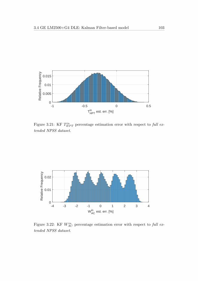
3.4 GE LM2500+G4 DLE: Kalman Filter-based model 103
-1 -0.5 0 0.5
THPTin est. err. [%]
0
0.005
0.01
0.015
Rel
ativ
e F
requ
ency
Figure 3.21: KF T inHPT percentage estimation error with respect to full ex-
tended NPSS dataset.
-4 -3 -2 -1 0 1 2 3 4
WACin est. err. [%]
0
0.01
0.02
Rel
ativ
e F
requ
ency
Figure 3.22: KF W inAC percentage estimation error with respect to full ex-
tended NPSS dataset.

104 Gas Turbine Modelling and Model-Based Estimation
-4 -3 -2 -1 0 1 2 3 4
WHPTin est. err. [%]
0
0.01
0.02
Rel
ativ
e F
requ
ency
Figure 3.23: KF W inHPT percentage estimation error with respect to full
extended NPSS dataset.
-3 -2 -1 0 1 2 3 4 5
WCCin est. err. [%]
0
0.01
0.02
Rel
ativ
e F
requ
ency
Figure 3.24: KF W inCC percentage estimation error with respect to full ex-
tended NPSS dataset.

3.5 Kalman Filter LHV estimation 105
Finally, it is immediate to notice that errors on flows estimations are
definitely greater with respect to the errors on temperatures estimations; this
is due to the fact that there are not suitable measurements that make the
proposed model directly aware about flows deviations from nominal values,
thus it is very complex to reduce these errors.
3.5 Kalman Filter LHV estimation
KF model estimation introduced in section 3.4 does not rely on equation
(3.9), indeed it exploits only the “backward” estimation of T inHPT provided
by equation (3.14). This feature of the KF can be exploited to allow the
estimation of an additional fundamental quantity, i.e. LHV.
LHV is a property of a fuel, and it is defined as the amount of heat
released by combusting a unit mass of fuel; thus, this quantity is needed to
characterised the fuel from an energetic point of view. LHV is very important
to control the GT, indeed its knowledge is required in order to compute
the exact quantity of fuel to be injected in combustion chamber. In fact
GT governor at first considers the nominal value LHV nom to compute the
normalised fuel request, then the actual fuel request is calculated multiplying
by the ratio LHV nom/LHV meas; if LHV meas > LHV nom it means that the
unit mass of fuel “contains” more energy, thus it is sufficient to inject a lower
fuel flow, on the contrary if LHV meas < LHV nom a greater quantity of fuel
is required.
By inverting equation (3.9) it is easy to achieve an estimation of LHV
based on the estimation of T inHPT provided by KF.
ˆLHV =1
ηCC
[T inHPT,KF ·
(cp,airAFR+ cp,fuel
)+
− Tfuel · cp,fuel − T outAC,KF ·AFR · cp,air] (3.23)
Where the bar over the variable states again that the quantity is directly
measured, while the additional subscript “KF” states that the quantity is
the estimation provided by KF.
106 Gas Turbine Modelling and Model-Based Estimation
The introduction of LHV estimation is very useful from two points of
view:
i. As explained in the previous sections an accurate knowledge of T inHPT
and LHV is fundamental to control the GT. T inHPT can not be mea-
sured and it needs to be estimated, while LHV is usually measured
by a gas chromatograph, that is a very complex and expensive trans-
ducer. This estimation method of LHV can be seen as a virtual sensor
able to work in parallel with the physical sensor (or even substitute it).
This soft sensor would bring many benefits, indeed it would increase
the operability and the reliability of the system, reducing at the same
time the total cost and instrumentation complexity;
ii. Concerning GG extended NPSS dataset and full extended NPSS dataset
both LHV and T inHPT numerical values are available, thus it is possible
to define an estimation error for both of them. In real trend datasets
the measured value of T inHPT is not available, thus it is necessary to
find out another index to evaluate the goodness of the method. LHV
is a perfect quantity to do this, indeed it is almost always available
on aero-derivative GTs and it is directly connected to T inHPT , thus it
is reasonable to suppose that if LHV estimation is accurate then also
the T inHPT estimation will be acceptable (even if it is not possible to
directly evaluate it).
3.5.1 Kalman Filter LHV estimation: results
Kalman Filter LHV estimation results with respect to GG ex-
tended NPSS dataset
Figure 3.25 represents the LHV percentage estimation error relative to GG
extended NPSS dataset. The error distribution is almost Gaussian and it
is not biased (µ ' 0%, σ ' 0.5%). Standing from equation (3.23) it is
clear that the estimation of LHV is strictly connected with the estimation
of T inHPT : the reason why the standard deviation of the distribution in figure

3.5 Kalman Filter LHV estimation 107
3.25 is significantly greater than the standard deviation of the distribution
in figure 3.15 is that equation (3.23) depends also on ηCC , thus it is much
more affected by the GG CPs.
-2 -1.5 -1 -0.5 0 0.5 1 1.5 2LHV est. err. [%]
0
0.02
0.04
0.06
0.08
Rel
ativ
e F
requ
ency
Figure 3.25: KF percentage error on LHV estimation with respect to GG
extended NPSS dataset.
Kalman Filter LHV estimation results with respect to full ex-
tended NPSS dataset
Figure 3.26 represents the LHV percentage estimation error relative to full
extended NPSS dataset. Once again, the distribution of figure 3.26 seems
to be the sum of several nearly-Gaussian distributions. The motivation, as
mentioned in paragraph 3.4.2, is that the proposed model-based on KF is
not able to follow the variations introduced by the CPs relative to LPT: this
means that KF is almost blind with respect to variations of LPT model, thus
the more it varies the more the error will grow.
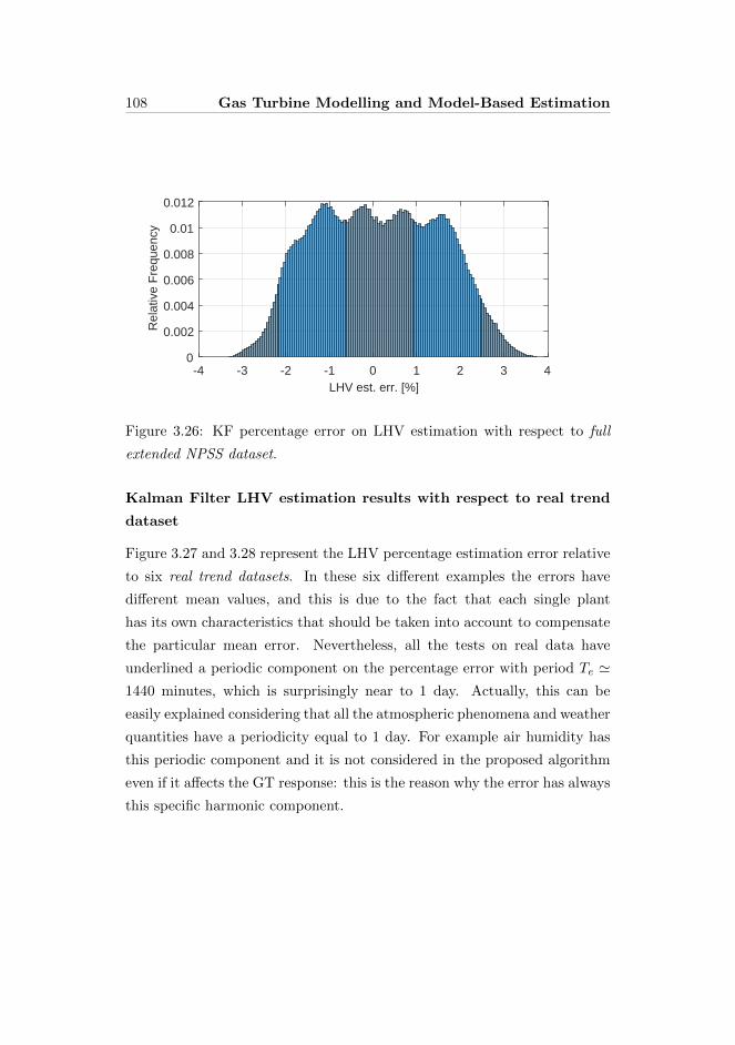
108 Gas Turbine Modelling and Model-Based Estimation
-4 -3 -2 -1 0 1 2 3 4LHV est. err. [%]
0
0.002
0.004
0.006
0.008
0.01
0.012
Rel
ativ
e F
requ
ency
Figure 3.26: KF percentage error on LHV estimation with respect to full
extended NPSS dataset.
Kalman Filter LHV estimation results with respect to real trend
dataset
Figure 3.27 and 3.28 represent the LHV percentage estimation error relative
to six real trend datasets. In these six different examples the errors have
different mean values, and this is due to the fact that each single plant
has its own characteristics that should be taken into account to compensate
the particular mean error. Nevertheless, all the tests on real data have
underlined a periodic component on the percentage error with period Te '1440 minutes, which is surprisingly near to 1 day. Actually, this can be
easily explained considering that all the atmospheric phenomena and weather
quantities have a periodicity equal to 1 day. For example air humidity has
this periodic component and it is not considered in the proposed algorithm
even if it affects the GT response: this is the reason why the error has always
this specific harmonic component.

3.5 Kalman Filter LHV estimation 109
0 2000 4000 6000 8000 10000Step #
-5
-4
-3
-2
-1
0
LHV
est
. err
. [%
]
(a) LHV estimation error with respect to gas chromatograph measurements (real
trend dataset 1).
0 500 1000 1500 2000Step #
-2
0
2
LHV
est
. err
. [%
]
(b) LHV estimation error with respect to gas chromatograph measurements (real
trend dataset 2).
0 0.5 1 1.5 2 2.5 3 3.5Step # 104
-2
0
2
4
LHV
est
. err
. [%
]
(c) LHV estimation error with respect to gas chromatograph measurements (real
trend dataset 3).
Figure 3.27: LHV estimation percentage errors (real trend datasets, 1Step
corresponds to 1minute).

110 Gas Turbine Modelling and Model-Based Estimation
0 0.5 1 1.5 2 2.5 3 3.5Step # 104
-1
0
1
2
3
LHV
est
. err
. [%
]
(a) LHV estimation error with respect to gas chromatograph measurements (real
trend dataset 4).
0 1000 2000 3000 4000 5000Step #
-6
-5
-4
-3
-2
LHV
est
. err
. [%
]
(b) LHV estimation error with respect to gas chromatograph measurements (real
trend dataset 5).
0 2000 4000 6000 8000 10000 12000Step #
-4
-2
0
2
LHV
est
. err
. [%
]
(c) LHV estimation error with respect to gas chromatograph measurements (real
trend dataset 6).
Figure 3.28: LHV estimation percentage errors (real trend datasets, 1Step
corresponds to 1minute).

3.6 Results analysis and conclusions 111
3.6 Results analysis and conclusions
In this chapter a suitable mathematical model of the aero-derivative twin-
shaft gas turbine GE LM2500+G4 DLE has been proposed. In particular,
the gas generator of this GT has been modelled introducing an iterative
double-step method:
1. the first step is based on generalised maps and thermodynamic laws
that allow an a-priori static estimation of flows, temperatures and pres-
sures of each GG section;
2. the second step provides dynamic estimations based on a Kalman Filter
that corrects the a-priori estimations exploiting all available measure-
ments and the thermodynamic/mechanical equilibrium of the system.
The model has been trained and validated with respect to several datasets
obtained exploiting NPSS. Moreover, concerning the estimation of LHV ,
also real trend datasets have been used to validate the GT mathematical
model.
The main results can be summarised as follows:
i. a-priori static model is able to reproduce the nominal NPSS dataset,
but it is characterised by large inaccuracies when the system moves far
away from the nominal one;
ii. the introduction of the second step based on KF allows the compen-
sation of many non-idealities of the system, above all regarding the
estimation of T inHPT . Figure 3.21 shows that the error with respect to
full extended NPSS datased has a Gaussian distribution with maximum
percentage value lower the 1%;
iii. in order to reduce installation costs, flow transducers are not available
in the GT under analysis. In turn, there are not direct measurements
that allow the reduction of the error on flows estimation, and this is
the reason why flows estimations are characterised by greater errors.

112 Gas Turbine Modelling and Model-Based Estimation
In view of the foregoing, the proposed model represents a comprehensive
method to describe the behaviour of the GT under analysis in all the rea-
sonable operating conditions, both in steady state and transient conditions.
This mathematical model can be used as soft sensor able to provide in-
direct measurement of LHV . This soft sensor has been validated also with
respect to real trend datasets, and results have shown that the estimation
error is composed of a systematic and a periodic component of 24 hours.
The former is due to modelling inaccuracies, while the second is linked to
the oscillation of meteorological quantities such as atmospheric humidity.
The goodness of the results paves the way for a wider field of application
of this approach. As mentioned previously, the immediate use of such a
model is as soft sensor to achieve indirect measurement of all the relevant
quantities that characterise the GT operating point. Concerning the usu-
ally unavailable measurements, this would lead to an increased awareness
about the whole system; among many unmeasured quantities, an accurate
estimation of T inHPT allows a more effective control of the machine, reducing
at the same time the amplitude of the margin needed to assure the physical
integrity of the system. Moreover, this soft sensor could also be used to
reduce the installation cost by estimating other quantities (such as LHV )
that are normally measured by expensive, bulk and invasive sensors that
generally need to be physically redounded. A second field of application
of this estimation method is the offline prediction of the GT performances:
this would guarantee a realistic evaluation of the GT response under specific
conditions without relying on a real running machine.
Finally, a deep knowledge about the system can help in estimating the
ageing and the physical decay of each engine component. Indeed, the aug-
mented knowledge about all the GT quantities can be exploited also to feed
proper algorithms to estimate the residual life of the system. An estimation
of the residual life closer to reality can be used to avoid premature and need-
less maintenance operations that on the contrary would be performed only
when strictly required.
Chapter 4
Conclusions and Final Remarks
The analysis and the techniques proposed in this work have highlighted
the potential of the model-based approach in oil and gas applications. A
mathematical model based on a deep knowledge of the system physics leads
to the improvement of existing oil and gas plants without requiring the
modification of already installed equipment.
As shown in Chapters 1 and 3, a reliable modelling of the particular
subsystem under analysis unlocks the full capabilities of the available equip-
ment. By introducing proper models focused on specific behaviour of the
system it is possible to develop suitable methods which are aimed to the
enhancement of the system reliability, operability and robustness. Thanks
to these models it is possible to compensate and overcome system lacks or
limitations without introducing expensive or overkill solution. A common
issue of many algorithms is that they are time consuming and high resources
demanding methods, thus they are scarcely applicable in a real plant. On
the contrary one of the main purposes of this work has been to keep each
algorithm “as simple as possible”. Indeed, each procedure has been con-
ceived to be able to work on a potentially available CPU, thus the run-time
complexity of each method should be as small as possible.
Furthermore, concerning the topic introduced in Chapter 2, the mathe-
matical modelization both of the mechanical and the electric part of a power
113

114 Conclusions and Final Remarks
generation plant has drawn the attention to the real features of the plant
that are at the basis of torsional instability. The awareness of the root causes
of this unstable phenomenon has allowed the implementation of an effective
mitigation technique able to force to system to maintain stability.
Nowadays, in order to keep pace with the scientific and technological
practices, it is clear that it is necessary to lean forward to embrace, develop
and rapidly adopt these new solutions. Model-based techniques indeed rep-
resent a unique opportunity to unleash the whole potential of the available
equipment without requiring additional and expensive installations.

Appendix A
Thermodynamics of Real Gases
Almost all of the gases handled by process practical applications (such as
compressors) are characterised by a pronounced real gas behaviour. This is
the reason why it is required to modify the well-known equation of perfect
gas introducing the parameter Z, i.e. the compressibility of the real gas.
Therefore, the real gas equation becomes
Z =pv
RT, (A.1)
where:
• Z is the gas compressibility;
• R ' 8.31 Jmol·K is the universal gas constant;
• p is the gas pressure;
• T is the gas temperature;
• v is the gas specific volume.
Note that Z ∈ [0; 1] is a pure number, and the perfect gas equation can be
achieved by imposing Z = 1.
In 1873 Van der Waals proposed the first technique to compute Z
Z =v
v − b− aRTv, (A.2)
115

116 Thermodynamics of Real Gases
with a and b coefficients to be determined connected to real gas peculiarities
and intermolecular dynamics.
In the second half of twentieth century many effective approaches to
calculate a generalised real gas equation of state have been introduced by
several scientists. Four real gas equations are described below.
A.1 BWRS equation of state
Benedict, Webb, Rubin and Starling published a new procedure to calculate
Z in 1973.
Z = 1 +B
v+C
v2+D
v5+E
v2
(1 +
γ
v2
)e−γ/v
2
, (A.3)
where
B =
(1
RT
)(B0RT −A0 −
C0
T 2+D0
T 3− E0
T 4
);
C =
(1
RT
)(bRT − a− d
T
);
D =
(1
RT
)α
(α+
d
T
);
D =
(1
RT
)(c
T 2
).
(A.4)
The unknown coefficients of equation (A.4) can be retrieved in [56].
A.2 RKS equation of state
Redlich, Kwong and Soave in 1949 suggested a modification to Van Der
Waals equation (A.2).
Z =v
v − b− a[
RT (v + b)] . (A.5)
Even in this case, unknown coefficients of equation (A.5) can be retrieved in
[56].

A.3 LKP equation of state 117
A.3 LKP equation of state
Lee, Kesler and Prausnitz proposed a new method to calculate Z in 1976.
Z = Z0 +ω
ωr(Zr − Z0). (A.6)
The compressibility factors of the ”simple fluid” Z0 and the ”reference
fluid” Zr are calculated separately by a modified BWRS equation. ωr repre-
sents the non-sphericity of a molecule, expressing how a molecule is complex
(geometry and polarity). ωr ranges from zero for simple monatomic gases
to approximately 0.9 for complex molecule structures.
In order to find out the numerical value of Z0 and Zr there are some
coefficients that can be retrieved in [56].
A.4 PR Equation of State
Peng and Robinson published their modification of the Van Der Waals equa-
tion (1976), known as the PR equation of state.
Z =v
v − b− v
RT
a[v(v + b) + b(v − b)
] . (A.7)
Once again, unknown coefficients of equation (A.7) can be retrieved in [56].

118 Thermodynamics of Real Gases

Appendix B
Least Squares Theory
Let’s consider the parametric linear model
Σ(ϑ): yk = ϕTk ϑ = ϕ1kϑ
1 + ϕ2kϑ
2 + · · ·+ ϕnkϑn, (B.1)
where:
• subscript k states that the quantity is referred to the k-th step;
• ϑ ∈ Rn is the coefficient vector that needs to be identified;
• ϕ ∈ Rn is the input vector;
• y ∈ R is the output value.
In practice, model (B.1) states that output y can be seen as a linear com-
bination of inputs. Identification of parameters vector ϑ is based on the
minimization of a cost function JN . If data are acquired in N steps, the cost
function is defined as
JN (ϑ) =1
N
N∑k=1
(yk −ϕTk ϑ)2, (B.2)
and the coefficient vector ϑ is equal to
ϑ ∈ argminϑJN (ϑ). (B.3)
There are two analytic methods to solve this minimization:
119

120 Least Squares Theory
1. Classic least squares: once all the data have been acquired from step
1 to step N , it computes vector ϑ (a complete analysis of classic least
squares can be found in many manuals such as [58], [27] or [25]);
2. Recursive least squares (RLS): step by step it updates the coefficient
vector ϑk, and it is possible to prove that ϑN is exactly equal to the
value ϑ that classic least squares method would return with the same
inputs (further details about RLS can be found e.g. in [42]).
B.1 Classic least squares
It is possible to demonstrate that the vector ϑ that minimises the cost func-
tion JN is equal to
ϑ = S(N)−1N∑k=1
ϕk yk, (B.4)
where
S(N) =
N∑k=1
ϕk ϕTk . (B.5)
B.2 Recursive least squares (RLS)
This method updates the estimation after each step by repeating the follow-
ing recursive equations (the algorithm can be initialised with the first step
data):
i. Sk = Sk−1 +ϕk ϕTk ;
ii. Kk = S−1k ϕk;
iii. εk = yk −ϕTk ϑk−1;
iv. ϑk = ϑk−1 +Kkεk.

B.2 Recursive least squares (RLS) 121
In practice, these equations are not used due to computational problems.
Indeed it is possible to define other equations mathematically equivalent to
these ones that avoid the calculation of inverse matrix. Theory ensures that
these new equations lead to the same result, but they are more robust from
a numerical and computational point of view:
i. βk−1 = 1 +ϕTk V k−1ϕk;
ii. V k = V k−1 − β−1k−1V k−1ϕkϕ
Tk V k−1;
iii. εk = yk −ϕTk ϑk−1;
iv. Kk = V kϕk;
v. ϑk = ϑk−1 +Kkεk.
Where the matrix V and the vector ϑ can be initialised with
V 0 =αI, α > 0
ϑ0 = 0.
In some special cases, it is useful to introduce a forgetting factor µ ∈ (0; 1]
(FF), that is a coefficient that allows the recursive least squares method to
be less influenced by the older data. Additional information about forgetting
factor RLS can be found in many handbooks or manuals, e.g. see [57] or
[10]. The forgetting factor makes the estimation more “nervous”, indeed it
is more influenced by the recent acquisitions and it forces the algorithm to
“forget” the older data. Defining the cost function in correspondence of the
k-th step as
Jk(ϑ) =1
N
k∑i=1
µk−i(yi −ϕTi ϑ)2, µ ∈ (0; 1]. (B.6)
The weighting factor µk−i reduces the influence of older errors on the esti-
mation.
The coefficient that minimises the cost function Jk can be achieved with
these recursive equations:

122 Least Squares Theory
i. βk−1 = µ+ϕTk V k−1ϕk;
ii. V k = µ−1(V k−1 − β−1k−1V k−1ϕkϕ
Tk V k−1);
iii. εk = yk −ϕTk ϑk−1;
iv. Kk = V kϕk;
v. ϑk = ϑk−1 +Kkεk.
On the contrary, if it is necessary to smooth the coefficient estimation,
a low-pass solution can be adopted. In practice, the coefficient vector ϑk is
estimated in the same way, but the final estimation is
ϑk = (1− λ)ϑk−1 + λϑk, (B.7)
where λ ∈ [0; 1]. The lower λ the higher the low pass effect.

Appendix C
Kalman Filter
This appendix provides a panoramic on Kalman Filter (KF), however further
details can be retrieved in many academic handbooks or articles, e.g. see
[51], [88], [35] and [22].
C.1 Kalman filtering: linear quadratic esti-
mation (LQE)
A discrete-time stochastic process Σ can be described by the system shown
in (C.1)
Σ :
xk+1 = fk(xk,uk,wk)
yk = hk(xk,ηk)(C.1)
where xk and uk are respectively the state and the input at time Tk, f(·) is
the function that describes the evolution of the state, h(·) is the observation
function and wk and ηk are the process and the observation noises.
If the process and the observation equations are linear equations both
with respect to the state xk, the input uk and the noises, then the process
123

124 Kalman Filter
Σ becomes:
Σ :
xk+1 = Akxk +Bkuk +Dkwk
yk = Ckxk + ηk
(C.2)
In the Kalman Filter theory, in addition to the linearity of the process,
there are also other fundamental assumptions:
• wk and ηk have to be white noises with covariance matrices equal to
Qk and Rk and expected value 0. This means that Ewk] = 0
E[wkwTi ] = Qkδk−i
,
E[ηk] = 0
E[ηkηTi ] = Rkδk−i
∀k, i ∈ Z
where δk−i is equal to 1 if k = i and equal to 0 in all the other cases.
These conditions are usually abbreviated as
wk ∼ wn(0,Qk) ηk ∼ wn(0,Rk)
• wk⊥ηk, so wk and ηk have to be uncorrelated between each other;
E[wkηTi ] = 0 ∀k, i ∈ Z
• the initial state x0 has to be a stochastic variable with expected value
x0 and covariance matrix P 0;
E[x0] = x0 E[x0xT0 ] = P 0
• x0⊥wk and x0⊥ηk, so the initial state x0 has to be uncorrelated with
wk and ηk
E[x0ηTk ] = 0, E[x0w
Tk ] = 0 ∀k ∈ Z.

C.1 Kalman filtering: linear quadratic estimation (LQE) 125
These last assumptions can be summarised in this way:
E
x0
wk
ηk
=
x0
0
0
, ∀k ∈ Z
E
x0
wk
ηk
[xT0 wTi ηTi
]=
P 0 0 0
0 Qkδk−i 0
0 0 Rkδk−i
, ∀k, i ∈ Z
(C.3)
Defining xk as the estimation of the state at k-th step, the estimation error
can be written as
xk = xk − xk. (C.4)
The idea of the Kalman Filter is to look for the estimation of the state that
in correspondence of each step minimises the Mean Square Error (MSE)
E[(xk − xk)(xk − xk)T ] = E[xkxTk ].
The previous mean square error is equal to the covariance matrix of the state
in the k-th step, that is P k = E[xkxTk ]. Considering the state observer
xk+1 = Akxk +Bkuk +Kk(yk −Ckxk)
and using the definition given in (C.4) it is possible to find out the value of
Kk that minimises P k ∀k. Indeed it is correct to write
xk+1 = xk+1 − xk+1 = Akxk +Bkuk +Dkwk −Akxk+
−Bkuk −Kk(yk −Ckxk)
and since yk = Ckxk + ηk, it yields
xk+1 =(Ak −KkCk
)xk +Dkwk −Kkηk.
Therefore, the mean square error P k+1 can be computed as
P k+1 = E[xk+1xTk+1] = E[
(Ak −KkCk
)xkx
Tk
(Ak −KkCk
)T]+
+ E[DkwkwTkD
Tk ] + E[Kkηkη
TkK
Tk ]

126 Kalman Filter
where the last equality is due to the fact that the variables are uncorrelated,
so the covariance of the sum is equal to the sum of the single covariances.
Therefore P k+1 is given by
P k+1 =(Ak −KkCk
)P k
(Ak −KkCk
)T+DkQkD
Tk +KkRkK
Tk .
As mentioned before Kk has to be computed as
Kk = arg minK
(Ak −KCk
)P k
(Ak −KCk
)T+DkQkD
Tk +KRkK
T
= arg min
K
K(Rk +CkP kC
Tk
)KT −KCkP kA
Tk −AkP kC
TkK
T+
AkP kATk +DkQkD
Tk
.
Defining Sk=Rk +CkP kCTk the previous equation becomes
Kk = arg minK
(K −AkP kC
TkS−1k
)Sk(K −AkP kC
TkS−1k
)T+M
.
Where M = AkP kATk +DkQkD
Tk −AkP kC
TkS−1k CkP kA
Tk does not de-
pend on K, so
Kk = arg minK
(K −AkP kC
TkS−1k
)Sk(K −AkP kC
TkS−1k
)T.
This equation finally leads to
Kk = AkP kCTkS−1k = AkP kC
Tk
(Rk +CkP kC
Tk
)−1. (C.5)
If Kk assumes the value described in (C.5), then P k+1 is equal to
P k+1 = AkP kATk +DkQkD
Tk −AkP kC
TkS−1k CkP kA
Tk =
= AkP kATk +DkQkD
Tk +
−AkP kCTk
(Rk +CkP kC
Tk
)CkP kA
Tk .
(C.6)
Therefore, the best estimation for xk+1 corresponding to P k+1 is
xk+1 =(Ak −KkCk
)xk +Bkuk −Kkyk =
= Akxk +Bkuk +Kk
(yk −Ckxk
).
(C.7)

C.1 Kalman filtering: linear quadratic estimation (LQE) 127
Variable Meaning
xk|k The updated state estimation at time
k given observations up to and includ-
ing time k
P k|k The updated error covariance matrix
(a measure of the accuracy of the state
estimation)
xk+1|k The predicted state estimation at time
k+ 1 given observations up to and in-
cluding time k
P k+1|k The predicted error covariance matrix
Table C.1: A new notation for the estimated state and its covariance matrix.
It should be noted that Kk can be also expressed as AkLk with Lk =
P kCTkS−1k . In this way it is possible to divide the whole algorithm in two
separated steps: prediction and updating.
Indeed, introducing the notation reported in table C.1, the (C.7) can be
written as
xk+1|k = Akxk +Bkuk +Kk
(yk −Ckxk
)=
= Ak
(xk|k−1 +Lk(yk −Ckxk|k−1)
)︸ ︷︷ ︸xk|k
+Bkuk. (C.8)
Similarly, it is possible to separate the calculus of the covariance matrix
P k+1 in a step of prediction and one step of updating.
P k+1|k = AkP kATk −AkLk︸ ︷︷ ︸
Kk
SkLTkA
Tk +DkQkDk =
= Ak
[P k|k−1 −LkSkLTk
]︸ ︷︷ ︸P k|k
ATk +DkQkD
Tk .
(C.9)
Using (C.8) and (C.9) it is possible to completely define the two steps of
prediction and updating as shown in C.2

128 Kalman Filter
Updating Prediction
xk|k = xk|k−1 +Lk(yk −Ckxk|k−1) xk+1|k = Akxk|k +Bkuk
P k|k = P k|k−1 −LkSkLk P k+1|k = AkP k|kATk +DkQkD
Tk
Table C.2: Updating and prediction step for the state estimation and its
covariance matrix.
Kalman filter algorithm
Therefore, the Kalman filter can be applied to reach the best estimation of
the state of the stochastic process Σ following these recursive steps:
1. the first step is necessary to define the initial condition of the state
estimation x1|0 and its covariance matrix P 1|0;
2. updating steps (for k = 1, 2, . . . )
Sk = Rk +CkP k|k−1CTk ;
Lk = P k|k−1CTkS−1k ;
ek = yk −Ckxk|k−1;
xk|k = xk|k−1 +Lkek;
P k|k =(I −LkCk
)P k|k−1
(I −LkCk
)T+LkRkL
Tk .
Where the last equation for P k|k is equivalent to the previous one,
even if this formulation is more robust for practical implementation;
3. prediction steps (for k = 1, 2, . . . )
xk+1|k = Akxk|k +Bkuk;
P k+1|k = AkP k|kATk +DkQkD
Tk .
Even in the case where the process Σ is stationary (Ak = A, Bk = B, Ck =
C, Dk = D, Qk = Q, Rk = R), the Kalman gain Kk is not constant,
indeed it would be equal to
Kk = AP kCT(R+CP kC
T)−1
. (C.10)
C.2 Approximated Kalman filter algorithm for non-linear process 129
To reach the optimal constant value for the Kalman gain K it is necessary to
introduce without demonstration that, under suitable hypothesis, a solution
to the Algebraic Riccati Equation is
P = ATPA−ATPB(R+BTPB)−1BTPA+Q
such that
limt→∞
P k = P ∀P 0.
It is possible to demonstrate that the observer with Kalman gain equal to
K = APCT(R+CPCT
)−1(C.11)
is the optimal observer with constant gain.
C.2 Approximated Kalman filter algorithm for
non-linear process
The classic Kalman filter algorithm has many assumptions. Some of these
assumptions, such as that the noises have to be zero-mean white noise mutu-
ally uncorrelated, can be relaxed changing the system. However the strongest
assumption is that the process Σ has to be linear. If Σ is not linear there
are many approximated methods that attempt to find the best estimation
of the state xk ∀k ∈ Z. Some of the most important methods are:
• Extended Kalman filter (EKF);
• Unscented Kalman filter (UKF);
• Particle filter (PF).
In the next paragraph the Extended Kalman filter (EKF) will be presented.
C.2.1 Extended Kalman filter (EKF)
This method considers a linear approximation of the process Σ around the
estimations of the state in order to transform the complete process Σ in a

130 Kalman Filter
linear process Σ which can be used in a classic Kalman filter. Let’s consider
a non-linear process Σ with additive noises such as
Σ :
xk+1 = fk(xk,uk) +wk
yk = hk(xk) + ηk
Moreover, concerning the updating steps, let consider the Taylor series of
the function hk(·) around the state estimation xk|k−1
hk(xk) = hk(xk|k−1) +∂hk∂xk
(xk|k−1)(xk − xk|k−1) + · · · '
' hk(xk|k−1) +Ck(xk − xk|k−1)
where
Ck =∂hk∂xk
(xk|k−1). (C.12)
In addition to this, concerning the prediction steps, let’s consider the Taylor
series of the function fk(·) in the neighbourhood of the state estimation xk|k
fk(xk) = fk(xk|k) +∂fk∂xk
(xk|k)(xk − xk|k) + · · · '
' fk(xk|k) +Ak(xk − xk|k)
where
Ak =∂fk∂xk
(xk|k). (C.13)
Once introduced these approximations, it is possible to define the EKF al-
gorithm suitable for all the non-linear process:
1. The first step is necessary to define the initial condition of the state
estimation x1|0 and his covariance matrix P 1|0. This algorithm does
not provide any guarantee of convergence, the only way to be quite
sure of reaching the convergence to the real state is to choose an initial
estimation as close as possible to the real one;

C.2 Approximated Kalman filter algorithm for non-linear process 131
2. updating steps (for k = 1, 2, . . . )
Sk = Rk +CkP k|k−1CTk ;
Lk = P k|k−1CTkS−1k ;
ek = yk − hk(xk|k−1);
xk|k = xk|k−1 +Lkek;
P k|k =(I −LkCk
)P k|k−1
(I −LkCk
)T+LkRkL
Tk .
3. prediction steps (for k = 1, 2, . . . )
xk+1|k = fk(xk|k);
P k+1|k = AkP k|kATk +QT
k .
where the last equation is due to the fact that Dk = 1.

132 Kalman Filter

Appendix D
Publications
International Journals
1. M. Basso, M. Galanti, G. Innocenti and D. Miceli, Pedestrian Dead Reck-
oning Based on Frequency Self-Synchronization and Body Kinematics, IEEE
Sensors Journal, vol. 17 , no. 2, pp. 534–545, Jan 2017.
URL: http://ieeexplore.ieee.org/stamp/stamp.jsp?tp=&arnumber=7752792&
isnumber=7792229
[DOI:10.1109/JSEN.2016.2631629]
Submitted
1. M. Basso, Matteo Galanti, G. Innocenti and D. Miceli.
Provisional paper title: Triggered INS/GNSS data fusion algorithms for en-
hanced pedestrian navigation system, IEEE Sensors Journal, 2018.
To be submitted
1. L. Alessandrini, M. Basso, Matteo Galanti, G. Innocenti, L. Giovanardi
and L. Pretini.
Provisional paper title: Maximum likelihood virtual firing temperature from
a thermodynamic internal model of a twin-shaft aeroderivative gas turbine,
Control System Technology, 2018.
133

134 Publications
Domestic Conferences
1. M. Galanti, M. Basso, G. Innocenti. “Pedestrian dead-reckoning based on
frequency self-synchronization and body kinematics”, in SIDRA, Automat-
ica.it 2018, Firenze (Italy), 12-14 Settembre 2018.

List of Figures
1.1 Example of axial compressor (a) and centrifugal compressor
casing (b). Courtesy of BHGE, source www.bhge.com . . . . . 8
1.2 Centrifugal compressor with vaned diffuser. . . . . . . . . . . 9
1.3 Impeller inlet and discharge velocity triangles. . . . . . . . . . 10
1.4 Typical turbocompressor performance map (black lines) and
a realistic load characteristic (grey line). . . . . . . . . . . . . 11
1.5 Centrifugal compressor schematic. . . . . . . . . . . . . . . . 13
1.6 Deviation with respect to case without noise using method
[A] (µ = −0.02%, σ = 1.92%). . . . . . . . . . . . . . . . . . . 18
1.7 Example of non-dimensional map of a centrifugal compressor. 20
1.8 Deviation with respect to case without noise using method
[B] (µ = −0.23%, σ = 1.51%). . . . . . . . . . . . . . . . . . . 21
1.9 Deviation with respect to case without noise using method
[C] (µ = −0.28%, σ = 2.71%). . . . . . . . . . . . . . . . . . . 23
1.10 Generic schematic of a torque-meter. . . . . . . . . . . . . . . 25
1.11 Percentage errors of centrifugal compressor power estimation
based on method [A] (blue line), method [B] (orange line) and
method [C] (yellow line). . . . . . . . . . . . . . . . . . . . . . 26
1.12 Schematic of method [C2]. . . . . . . . . . . . . . . . . . . . . 29
1.13 Percentage errors of centrifugal compressor power estimation
based on method [C] (blue line) and method [C2] (orange line). 30
1.14 Schematic of Td absolute estimation based on least squares
theory. . . . . . . . . . . . . . . . . . . . . . . . . . . . . . . . 33
135
136 LIST OF FIGURES
1.15 Percentage errors of absolute estimations based on least squares
theory. Blue line (10% of total data) refers to calibration
phase, while orange line (last 90% of data) refers to valida-
tion interval. . . . . . . . . . . . . . . . . . . . . . . . . . . . 35
1.16 Percentage errors of thermodynamic predictions. . . . . . . . 37
1.17 Schematic of Td prediction error estimation based on RLS
theory. . . . . . . . . . . . . . . . . . . . . . . . . . . . . . . . 38
1.18 Percentage errors obtained estimating the thermodynamic pre-
diction error with RLS. Blue line (10% of total data) refers to
calibration phase, while orange line (last 90% of data) refers
to validation interval. . . . . . . . . . . . . . . . . . . . . . . . 40
2.1 Schematic explanation of SSTI phenomenon. . . . . . . . . . 44
2.2 Physical model of TG shaft. . . . . . . . . . . . . . . . . . . . 46
2.3 Frequency analysis of SSTI phenomenon (example). The fig-
ure is composed of two rows and two columns: first row is
relative to time domain while the second is relative to fre-
quency domain, first column is relative to current while the
second is relative to power. . . . . . . . . . . . . . . . . . . . 51
2.4 Schematic of SSTI mitigation system. . . . . . . . . . . . . . 53
2.5 Schematic of SSTI damping system. . . . . . . . . . . . . . . 54
2.6 Schematic of electric power generation and distribution system. 57
2.7 Simulation results of three examples of torsional oscillations
damping. . . . . . . . . . . . . . . . . . . . . . . . . . . . . . 58
2.8 Example of damper line currents and DC link current. . . . . 60
3.1 Single-shaft GT schematic. . . . . . . . . . . . . . . . . . . . 67
3.2 Two-shaft GT with separated power turbine schematic. . . . 67
3.3 GE LM2500+G4, a two-shaft aero-derivative GT. This GT
belongs to GE LM series, where LM states for Land & Marine.
Courtesy of BHGE (source www.bhge.com). . . . . . . . . . . 68

LIST OF FIGURES 137
3.4 Two different views of a single-shaft GT. Courtesy of BHGE
(source www.ge.com). . . . . . . . . . . . . . . . . . . . . . . . 69
3.5 Schematic representation of ideal/real Brayton cycle of a single-
shaft GT. . . . . . . . . . . . . . . . . . . . . . . . . . . . . . 72
3.6 NPSS temperatures percentage deviation: full extended NPSS
dataset versus nominal NPSS dataset. . . . . . . . . . . . . . 75
3.7 NPSS flows percentage deviation: full extended NPSS dataset
versus nominal NPSS dataset. . . . . . . . . . . . . . . . . . . 76
3.8 AC flow coefficient map. . . . . . . . . . . . . . . . . . . . . . 81
3.9 AC isentropic efficiency map. . . . . . . . . . . . . . . . . . . 83
3.10 kp,drop map. . . . . . . . . . . . . . . . . . . . . . . . . . . . . 85
3.11 A-priori static T inHPT percentage estimation error with respect
to full extended NPSS dataset. . . . . . . . . . . . . . . . . . . 88
3.12 Schematic of GT estimation based on Kalman Filter. . . . . . 90
3.13 KF T outAC percentage estimation error with respect to GG ex-
tended NPSS dataset. . . . . . . . . . . . . . . . . . . . . . . . 98
3.14 KF T outHPT percentage estimation error with respect to GG
extended NPSS dataset. . . . . . . . . . . . . . . . . . . . . . 99
3.15 KF T inHPT percentage estimation error with respect to GG
extended NPSS dataset. . . . . . . . . . . . . . . . . . . . . . 99
3.16 KF W inAC percentage estimation error with respect to GG ex-
tended NPSS dataset. . . . . . . . . . . . . . . . . . . . . . . . 100
3.17 KF W inHPT percentage estimation error with respect to GG
extended NPSS dataset. . . . . . . . . . . . . . . . . . . . . . 100
3.18 KF W inCC percentage estimation error with respect to GG ex-
tended NPSS dataset. . . . . . . . . . . . . . . . . . . . . . . . 101
3.19 KF T outAC percentage estimation error with respect to full ex-
tended NPSS dataset. . . . . . . . . . . . . . . . . . . . . . . . 102
3.20 KF T outHPT percentage estimation error with respect to full ex-
tended NPSS dataset. . . . . . . . . . . . . . . . . . . . . . . . 102
3.21 KF T inHPT percentage estimation error with respect to full ex-
tended NPSS dataset. . . . . . . . . . . . . . . . . . . . . . . . 103

138 LIST OF FIGURES
3.22 KF W inAC percentage estimation error with respect to full ex-
tended NPSS dataset. . . . . . . . . . . . . . . . . . . . . . . . 103
3.23 KF W inHPT percentage estimation error with respect to full
extended NPSS dataset. . . . . . . . . . . . . . . . . . . . . . 104
3.24 KF W inCC percentage estimation error with respect to full ex-
tended NPSS dataset. . . . . . . . . . . . . . . . . . . . . . . . 104
3.25 KF percentage error on LHV estimation with respect to GG
extended NPSS dataset. . . . . . . . . . . . . . . . . . . . . . 107
3.26 KF percentage error on LHV estimation with respect to full
extended NPSS dataset. . . . . . . . . . . . . . . . . . . . . . 108
3.27 LHV estimation percentage errors (real trend datasets, 1Step
corresponds to 1minute). . . . . . . . . . . . . . . . . . . . . 109
3.28 LHV estimation percentage errors (real trend datasets, 1Step
corresponds to 1minute). . . . . . . . . . . . . . . . . . . . . 110

List of Tables
1.1 Centrifugal compressor quantities nomenclature . . . . . . . . 14
1.2 Outcomes of sensitivity analysis of methods [A], [B] and [C]. . 24
3.1 LM2500 GT family characteristics. . . . . . . . . . . . . . . . 71
3.2 GE LM2500+G4 DLE main quantities nomenclature . . . . . 79
3.3 Inputs and outputs of the proposed AC model. . . . . . . . . 80
3.4 Inputs and outputs of the proposed combustion chamber model. 84
3.5 Inputs and outputs of the proposed HPT model. . . . . . . . 87
C.1 A new notation for the estimated state and its covariance
matrix. . . . . . . . . . . . . . . . . . . . . . . . . . . . . . . . 127
C.2 Updating and prediction step for the state estimation and its
covariance matrix. . . . . . . . . . . . . . . . . . . . . . . . . 128
139

140 LIST OF TABLES

Bibliography
[1] T. Addabbo, R. Biondi, S. Cioncolini, A. Fort, F. Rossetti, and V. Vignoli,
“A zero-crossing detection system based on FPGA to measure the angular
vibrations of rotating shafts,” IEEE Transactions on Instrumentation and
Measurement, vol. 63, no. 12, pp. 3002–3010, Dec 2014.
[2] T. Addabbo, A. Fort, R. Biondi, S. Cioncolini, M. Mugnaini, S. Rocchi, and
V. Vignoli, “Measurement of angular vibrations in rotating shafts: Effects
of the measurement setup nonidealities,” IEEE Transactions on Instrumen-
tation and Measurement, vol. 62, no. 3, pp. 532–543, March 2013.
[3] R. Adhami, P. Meenen, and D. Hite, Fundamental Concepts in Electrical
and Computer Engineering with Practical Design Problems. Universal
Publishers, 2007. [Online]. Available: https://books.google.it/books?id=
9nqkVbFPutYC
[4] K. H. Ang, G. Chong, and Y. Li, “Pid control system analysis, design, and
technology,” IEEE Transactions on Control Systems Technology, vol. 13,
no. 4, pp. 559–576, July 2005.
[5] J. Angeles, Dynamic Response of Linear Mechanical Systems: Mod-
eling, Analysis and Simulation, ser. Mechanical Engineering Series.
Springer US, 2011. [Online]. Available: https://books.google.ch/books?id=
kn7p65y3uwUC
[6] M. Antonova, E. Vasilieva, and I. Zhezhera, “The antisurge protection of a
centrifugal compressor,” in 2017 International Conference on Modern Elec-
trical and Energy Systems (MEES), Nov 2017, pp. 80–83.
[7] G. Baldini, S. Bittanti, A. D. Marco, F. Longhi, G. Poncia, W. Prandoni,
and D. Vettorello, “A dynamic model of moving flames for the analysis and
141

142 BIBLIOGRAPHY
control of combustion instabilities,” in 1999 European Control Conference
(ECC), Aug 1999, pp. 2795–2800.
[8] A. Banaszuk, Y. Zhang, and C. A. Jacobson, “Adaptive control of combus-
tion instability using extremum-seeking,” in Proceedings of the 2000 Amer-
ican Control Conference. ACC (IEEE Cat. No.00CH36334), vol. 1, no. 6,
June 2000, pp. 416–422 vol.1.
[9] M. Bandyopadhyay, Electrical power system: Theory and Practice, ser.
Eastern Economy Edition. PHI Learning, 2006. [Online]. Available:
https://books.google.it/books?id=lrQJ kzGapUC
[10] C. Banyasz, Adaptive Systems in Control and Signal Processing 1995,
ser. IFAC Postprint Volume. Elsevier Science, 2014. [Online]. Available:
https://books.google.ch/books?id=g9HSBQAAQBAJ
[11] R. Bazyar, M. R. Javadi, A. Ghasemi, and A. Yusefi, “Analysis and study
subsynchronous resonance (SSR) in tabriz thermal power plant using thyris-
tor controlled series compensator,” in The 3rd Conference on Thermal Power
Plants, Oct 2011, pp. 1–5.
[12] K. Belmokhtar, H. Ibrahim, and A. Merabet, “Online parameter identifica-
tion for a dfig driven wind turbine generator based on recursive least squares
algorithm,” in 2015 IEEE 28th Canadian Conference on Electrical and Com-
puter Engineering (CCECE), May 2015, pp. 965–969.
[13] C. Bitikofer, M. P. Schoen, J. Li, and F. Lin, “Characteristic moore-greitzer
model parameter identification for a one stage axial compressor system,” in
2017 American Control Conference (ACC), May 2017, pp. 164–169.
[14] M. Boles and D. Yunus A. Cengel, Thermodynamics: An Engineering
Approach. McGraw-Hill Education, 2014. [Online]. Available: https:
//books.google.it/books?id=Ao95ngEACAAJ
[15] S. Borguet and O. Leonard, “Comparison of adaptive filters for
gas turbine performance monitoring,” Journal of Computational and
Applied Mathematics, vol. 234, no. 7, pp. 2202 – 2212, 2010,
fourth International Conference on Advanced COmputational Methods
in ENgineering (ACOMEN 2008). [Online]. Available: http://www.
sciencedirect.com/science/article/pii/S0377042709005561

BIBLIOGRAPHY 143
[16] M. Boyce, Gas Turbine Engineering Handbook. Elsevier Science, 2017.
[Online]. Available: https://books.google.it/books?id=zPAFHyHctRUC
[17] B. J. Brunell, R. R. Bitmead, and A. J. Connolly, “Nonlinear model predic-
tive control of an aircraft gas turbine engine,” in Proceedings of the 41st IEEE
Conference on Decision and Control, 2002., vol. 4, Dec 2002, pp. 4649–4651
vol.4.
[18] F. Caifen, T. Wen, and L. Jizhen, “Imc control of combustion instability,”
in 2008 27th Chinese Control Conference, July 2008, pp. 39–43.
[19] D. Childs and D. Childs, Turbomachinery Rotordynamics: Phenomena,
Modeling, and Analysis, ser. Wiley-Interscience publication. Wiley, 1993.
[Online]. Available: https://books.google.it/books?id=vKPfBxgQQPoC
[20] J. Chin and J. Csank, “Tool for the Integrated Dynamic Numerical Propul-
sion System Simulation (NPSS)/Turbine Engine Closed-Loop Transient
Analysis (TTECTrA),” National Aeronautics and Space Administration
(NASA), Glenn Research Center, Tech. Rep., 2016.
[21] F. Chu, B. Dai, W. Dai, R. Jia, X. Ma, and F. Wang, “Rapid modeling
method for performance prediction of centrifugal compressor based on model
migration and SVM,” IEEE Access, vol. 5, pp. 21 488–21 496, 2017.
[22] C. K. Chui and G. Chen, Kalman Filtering with Real-time Applications.
Berlin, Heidelberg: Springer Verlag, 1987.
[23] T. A. Clifford, S. Cruz-Manzo, Y. Zhang, V. Panov, and A. Latimer, “De-
velopment of a steady-state thermodynamic model in microsoft excel for
performance analysis of industrial gas turbines,” in IECON 2017 - 43rd An-
nual Conference of the IEEE Industrial Electronics Society, Oct 2017, pp.
4717–4723.
[24] H. Cohen, G. Rogers, P. Straznicky, H. Saravanamuttoo, and A. Nix, Gas
Turbine Theory. Pearson Education Limited, 2017. [Online]. Available:
https://books.google.it/books?id=hvEmDwAAQBAJ
[25] M. Dapor and M. Ropele, Elaborazione dei dati sperimentali, ser. UNITEXT.
Springer Milan, 2006. [Online]. Available: https://books.google.ch/books?
id=8RpLiEzqxRIC
[26] N. Daroogheh, N. Meskin, and K. Khorasani, “Ensemble kalman filters for
state estimation and prediction of two-time scale nonlinear systems with

144 BIBLIOGRAPHY
application to gas turbine engines,” IEEE Transactions on Control Systems
Technology, pp. 1–9, 2018.
[27] A. Ferrero, Esposizione del Metodo dei Minimi Quadrati (Classic Reprint).
Fb&c Limited, 2018. [Online]. Available: https://books.google.ch/books?
id=FmFRswEACAAJ
[28] D. Fontaine, S. Liao, J. Paduano, and P. V. Kokotovic, “Nonlinear control
experiments on an axial flow compressor,” IEEE Transactions on Control
Systems Technology, vol. 12, no. 5, pp. 683–693, Sept 2004.
[29] LM2500 - Marine Gas Turbine, GE Aviation, 2 2017. [Online]. Available:
https://www.geaviation.com/sites/default/files/datasheet-lm2500.pdf
[30] LM2500+ - Marine Gas Turbine, GE Aviation, 2 2017. [Online]. Available:
https://www.geaviation.com/sites/default/files/datasheet-lm2500plus.pdf
[31] LM2500+G4 - Marine Gas Turbine, GE Aviation, 2 2017.
[Online]. Available: https://www.geaviation.com/sites/default/files/
datasheet-lm2500plusg4.pdf
[32] T. Giampaolo, Gas Turbine Handbook: Principles and Practice.
Fairmont Press, 2009. [Online]. Available: https://books.google.it/books?
id=WbzGUYJEmdUC
[33] T. Goodman, “A least-squares method for computing balance corrections,”
Journal of Engineering for Industry, vol. 86, pp. 273–277, 1964.
[34] J. T. Gravdahl and O. Egeland, “A moore-greitzer axial compressor model
with spool dynamics,” in Proceedings of the 36th IEEE Conference on Deci-
sion and Control, vol. 5, Dec 1997, pp. 4714–4719 vol.5.
[35] M. S. Grewal and A. P. Andrews, Kalman Filtering: Theory and Practice
with MATLAB, 4th ed. Wiley IEEE Press, 2014.
[36] G. Gu, S. Banda, and A. Sparks, “An overview of rotating stall and surge
control for axial flow compressors,” in Proceedings of 35th IEEE Conference
on Decision and Control, vol. 3, Dec 1996, pp. 2786–2791 vol.3.
[37] D. H. Cooke, “On Prediction of Off Design Multistage Turbine Pressures by
Stodola’s Ellipse,” vol. 107, 07 1985.
[38] W. M. Haddad, A. Leonessa, V. S. Chellaboina, and J. L. Fausz, “Nonlin-
ear robust disturbance rejection controllers for rotating stall and surge in

BIBLIOGRAPHY 145
axial flow compressors,” IEEE Transactions on Control Systems Technology,
vol. 7, no. 3, pp. 391–398, May 1999.
[39] C. Hall and S. Dixon, Fluid Mechanics and Thermodynamics of
Turbomachinery. Elsevier Science, 2013. [Online]. Available: https:
//books.google.it/books?id=wZoTAAAAQBAJ
[40] H. Hanachi, J. Liu, A. Banerjee, Y. Chen, and A. Koul, “A physics-based
modeling approach for performance monitoring in gas turbine engines,”
IEEE Transactions on Reliability, vol. 64, no. 1, pp. 197–205, March 2015.
[41] L. Harnefors, “Analysis of subsynchronous torsional interaction with power
electronic converters,” IEEE Transactions on Power Systems, vol. 22, no. 1,
pp. 305–313, Feb 2007.
[42] M. Hayes, Statistical Digital Signal Processing and Modeling. Wiley India
Pvt. Limited, 2009. [Online]. Available: https://books.google.ch/books?id=
z0GqhOe9GNQC
[43] J. V. Helvoirt, “Centrifugal compressor surge: Modeling and identification
for control,” Ph.D. dissertation, Technische Universiteit Eindhoven, 2007.
[44] F. Iliceto, Impianti elettrici, ser. Impianti elettrici. Patron, 1984, no. Bd.
1. [Online]. Available: https://books.google.it/books?id=Uf2YPQAACAAJ
[45] M. R. Iravani, B. L. Agrawal, D. H. Baker, C. E. J. Bowler, R. G. Farmer,
R. A. Hedin, E. H. V. Larsen, and J. F. Tang, “Fourth supplement to a bib-
liography for the study of subsynchronous resonance between rotating ma-
chines and power systems,” IEEE Transactions on Power Systems, vol. 12,
no. 3, pp. 1276–1282, Aug 1997.
[46] G. D. Jennings, R. Harley, and B. S. Rigby, “Modal parameters and turbo-
generator torsional behavior,” in 3D Africon Conference. Africon ’92 Pro-
ceedings (Cat. No.92CH3215), Sept 1992, pp. 517–520.
[47] Z. Jian, H. K. Mathews, P. G. Bonanni, and S. Ruijie, “Model-based sen-
sor fault detection and isolation in gas turbine,” in Proceedings of the 31st
Chinese Control Conference, July 2012, pp. 5215–5218.
[48] M. Johnson and M. Moradi, PID Control: New Identification and Design
Methods, ser. Probability and its applications. Springer London, 2006.
[Online]. Available: https://books.google.ch/books?id=hY6oLlqLCv8C

146 BIBLIOGRAPHY
[49] S. Jones, “An Introduction to Thermodynamic Performance Analysis of Air-
craft Gas Turbine Engine Cycles Using the Numerical Propulsion System
Simulation Code,” National Aeronautics and Space Administration (NASA),
Glenn Research Center, Tech. Rep., 2007.
[50] F. Jurado, N. Acero, and A. Echarri, “Enhancing the electric system stability
using predictive control of gas turbines,” in 2006 Canadian Conference on
Electrical and Computer Engineering, May 2006, pp. 438–441.
[51] R. E. Kalman, “A New Approach to Linear Filtering and Prediction
Problems,” Transactions of the ASME, Journal of Basic Engineering,
no. 82 (Series D), pp. 35–45, 1960. [Online]. Available: http:
//www.cs.unc.edu/∼welch/kalman/media/pdf/Kalman1960.pdf
[52] C. Kasemann, L. van Lieshout, M. Huart, and M. Rott, “10MVA thyristor
converters for the active damping of generator shaft oscillations at ASDEX
upgrade,” Fusion Engineering and Design, vol. 84, no. 2, pp. 998 – 1001, 2009,
proceeding of the 25th Symposium on Fusion Technology. [Online]. Available:
http://www.sciencedirect.com/science/article/pii/S0920379608004924
[53] A. G. Kaviri and M. N. M. Jaafar, “Thermodynamic modeling and exergy
optimization of a gas turbine power plant,” in 2011 IEEE 3rd International
Conference on Communication Software and Networks, May 2011, pp. 366–
370.
[54] R. Khalili and M. Karrari, “Modeling and identification of an industrial
gas turbine using classical and non-classical approaches,” in 2017 Iranian
Conference on Electrical Engineering (ICEE), May 2017, pp. 667–672.
[55] D. Klein and C. Abeykoon, “Modelling of a turbojet gas turbine engine,” in
2015 Internet Technologies and Applications (ITA), Sept 2015, pp. 200–206.
[56] H. Knapp, R. Doring, L. Oellrich, U. Plocker, J. Prausnitz, R. Langhorst,
and Z. R., Vapor-Liquid Equilibria for Mixtures of Low Boiling Substances.
Chemistry Data Series, 1982.
[57] B. Kovacevic, Z. Banjac, and M. Milosavljevic, Adaptive Digital Filters,
ser. SpringerLink : Bucher. Springer Berlin Heidelberg, 2013. [Online].
Available: https://books.google.ch/books?id=LY7PQQGWr1kC

BIBLIOGRAPHY 147
[58] J. Leader, Numerical Analysis and Scientific Computation, ser. Featured
Titles for Numerical Analysis. Pearson Addison Wesley, 2004. [Online].
Available: https://books.google.ch/books?id=Q7tsNwAACAAJ
[59] G. Li, Z. Lin, C. Untaroiu, and P. E. Allaire, “Balancing of high-speed
rotating machinery using convex optimization,” in 42nd IEEE International
Conference on Decision and Control (IEEE Cat. No.03CH37475), vol. 4, Dec
2003, pp. 4351–4356 vol.4.
[60] G. Lin, “Flow meter system error treatment based on iterative learning con-
trol,” in 2011 Chinese Control and Decision Conference (CCDC), May 2011,
pp. 3777–3780.
[61] K. H. Ludtke, Process Centrifugal Compressors. Springer, 2004.
[62] J. Lytle, “The Numerical Propulsion System Simulation: A Multidisciplinary
Design System for Aerospace Vehicles,” National Aeronautics and Space
Administration (NASA), Glenn Research Center, Tech. Rep., 1999.
[63] C. A. Mansoux, D. L. Gysling, J. D. Setiawan, and J. D. Paduano, “Dis-
tributed nonlinear modeling and stability analysis of axial compressor stall
and surge,” in Proceedings of 1994 American Control Conference - ACC ’94,
vol. 2, June 1994, pp. 2305–2316 vol.2.
[64] K. R. McManus, J. C. Magill, and M. F. Miller, “Control of unsta-
ble combustion oscillations in liquid-fueled gas turbines,” in Proceedings
of the 1998 IEEE International Conference on Control Applications (Cat.
No.98CH36104), vol. 2, Sept 1998, pp. 1170–1174 vol.2.
[65] A. Mehta, H. Kaufman, and R. Ravi, “Turbine system identification: exper-
imental results,” in Proceedings of 1994 33rd IEEE Conference on Decision
and Control, vol. 4, Dec 1994, pp. 3593–3595 vol.4.
[66] F. Moore and E. Greitzer, “A theory of post-stall transients in axial com-
pressors: Part I - development of the equations,” in J. Eng.Gas Turbines
and Power, vol. 108, 1986, pp. 68–76 vol.108.
[67] F. Moore and M. Greitzer, “A theory of post-stall transients in axial com-
pressors: Part 2 - application,” in J. Eng.Gas Turbines and Power, vol. 108,
1986, pp. 231–239 vol.108.

148 BIBLIOGRAPHY
[68] D. Mudroncik, P. Tanuska, and M. Galik, “Surge control of natural gas cen-
trifugal compressor,” in 2009 Second International Conference on Computer
and Electrical Engineering, vol. 1, Dec 2009, pp. 110–113.
[69] D. Newland, Mechanical Vibration Analysis and Computation, ser. Dover
books on engineering. Dover Publications, 2013. [Online]. Available:
https://books.google.ch/books?id=LSrEAgAAQBAJ
[70] M. Nieuwenhuizen, J. van Helvoirt, and M. Steinbuch, “An analogy between
the Van der Pol equation and the Greitzer model,” in 2009 European Control
Conference (ECC), Aug 2009, pp. 490–495.
[71] D. Niu, A. Shi, Y. Chang, and F. Wang, “Modelling of multistage centrifugal
compressor,” in Proceedings of 2011 International Conference on Computer
Science and Network Technology, vol. 2, Dec 2011, pp. 1144–1147.
[72] C. Osnaghi, Teoria delle turbomacchine. Esculapio, 2013. [Online].
Available: https://books.google.it/books?id=3cMEAQAAQBAJ
[73] W. Peng, Fundamentals of Turbomachinery. Wiley, 2008. [Online].
Available: https://books.google.it/books?id=PEV3570XWR0C
[74] N. Petchers, Combined Heating, Cooling & Power Handbook: Technologies
& Applications : an Integrated Approach to Energy Resource Optimization.
Fairmont Press, 2003. [Online]. Available: https://books.google.it/books?
id=hA129h8dc1AC
[75] PLECS - The simulation platform for power electronic systems, PLEXIM
Electrical Engineering Software, 4 2018, rev. 4.1. [Online]. Available:
https://www.plexim.com/download/documentation
[76] M. Plis and H. Rusinowski, “Mathematical modeling of an axial compressor
in a gas turbine cycle,” Journal of Power Technologies, vol. 96, no. 3, pp.
194 – 199, 2016.
[77] B. Pourbabaee, N. Meskin, and K. Khorasani, “Sensor fault detection, isola-
tion, and identification using multiple-model-based hybrid kalman filter for
gas turbine engines,” IEEE Transactions on Control Systems Technology,
vol. 24, no. 4, pp. 1184–1200, July 2016.
[78] J. M. Protz and J. D. Paduano, “Rotating stall and surge: alternate mod-
eling and control concepts,” in Proceedings of the 1997 IEEE International
Conference on Control Applications, Oct 1997, pp. 866–873.

BIBLIOGRAPHY 149
[79] S. Purushothaman and F. de Leon, “Eliminating subsynchronous oscillations
with an induction machine damping unit (imdu),” IEEE Transactions on
Power Systems, vol. 26, no. 1, pp. 225–232, Feb 2011.
[80] A. Pytel and A. Kozk, “Modelling and effective predictive control of gas
turbine process,” in Proceedings of the 2014 15th International Carpathian
Control Conference (ICCC), May 2014, pp. 469–474.
[81] W. Qu and J. Jiang, “SSTI and its mitigation in wind farms connected
with an HVDC line,” Procedia Computer Science, vol. 111, pp. 399 –
405, 2017, the 8th International Conference on Advances in Information
Technology. [Online]. Available: http://www.sciencedirect.com/science/
article/pii/S1877050917312139
[82] W. M. Salim and S. A. Ahmed, “Numerical analysis of free vortex flow
in a combustor model,” in 2017 7th International Conference on Modeling,
Simulation, and Applied Optimization (ICMSAO), April 2017, pp. 1–5.
[83] G. C. Sarbu, “Modern water flowmeters: Differential pressure flowmeters,”
in 2016 International Conference and Exposition on Electrical and Power
Engineering (EPE), Oct 2016, pp. 609–616.
[84] A. S. Shiriaev, L. B. Freidovich, A. Robertsson, A. Andersson, and R. Jo-
hansson, “Sufficient conditions for dynamic stabilization of 3-state Moore-
Greitzer compressor model,” in 2015 54th IEEE Conference on Decision and
Control (CDC), Dec 2015, pp. 4394–4399.
[85] C. Sihler and T. Zoller, “Active damping of torsional modes in turbine-
generator shafts,” 08 2018.
[86] A. Sinha, Vibration of Mechanical Systems. Cambridge University
Press, 2010. [Online]. Available: https://books.google.ch/books?id=
hMPHTFfBt5oC
[87] C. Soares, Gas Turbines: A Handbook of Air, Land and Sea Applications.
Elsevier Science, 2014. [Online]. Available: https://books.google.it/books?
id=ubJZAwAAQBAJ
[88] H. Sorenson, Kalman Filtering: Theory and Application, ser. IEEE
Press selected reprint series. IEEE Press, 1985. [Online]. Available:
https://books.google.it/books?id=2pgeAQAAIAAJ
150 BIBLIOGRAPHY
[89] S. Strogatz, Nonlinear Dynamics And Chaos, ser. Studies in nonlinearity.
Sarat Book House, 2007. [Online]. Available: https://books.google.ch/
books?id=PHmED2xxrE8C
[90] F. Svetti, P. Rotondo, D. Sgro, and F. Meucci, “Practical guidelines for Oil &
Gas plant design against sub-synchronous torsional interaction phenomena,”
Turbomachinery Laboratories, Texas A&M Engineering Experiment Station,
2015.
[91] A. Tabesh and R. Iravani, “Frequency-response analysis of torsional dynam-
ics,” IEEE Transactions on Power Systems, vol. 19, no. 3, pp. 1430–1437,
Aug 2004.
[92] N. Thomopoulos, Statistical Distributions: Applications and Parameter
Estimates. Springer International Publishing, 2017. [Online]. Available:
https://books.google.ch/books?id=lng5DwAAQBAJ
[93] Torquemeters Limited, “Continuous duty torque measurement,”
https://www.torquemeters.com/wp-content/uploads/2013/03/
Continuous Duty Brochure.pdf, [Online; accessed 06-August-2018].
[94] G. Torrisi, S. Grammatico, A. Cortinovis, M. Mercangoz, M. Morari, and
R. S. Smith, “Model predictive approaches for active surge control in cen-
trifugal compressors,” IEEE Transactions on Control Systems Technology,
vol. 25, no. 6, pp. 1947–1960, Nov 2017.
[95] C. Tournes and D. B. Landrum, “Development of a physically based axial
compressor model,” in Proceedings of Thirtieth Southeastern Symposium on
System Theory, March 1998, pp. 120–124.
[96] J. van Helvoirt, B. de Jager, M. Steinbuch, and J. Smeulers, “Modeling and
identification of centrifugal compressor dynamics with approximate realiza-
tions,” in Proceedings of 2005 IEEE Conference on Control Applications,
2005. CCA 2005., Aug 2005, pp. 1441–1447.
[97] J. van Helvoirt and B. de Jager, “Dynamic model including piping
acoustics of a centrifugal compression system,” Journal of Sound and
Vibration, vol. 302, no. 1, pp. 361 – 378, 2007. [Online]. Available:
http://www.sciencedirect.com/science/article/pii/S0022460X06008820
BIBLIOGRAPHY 151
[98] A. Visioli, Practical PID Control, ser. Advances in Industrial Control.
Springer London, 2006. [Online]. Available: https://books.google.ch/books?
id=ymyAY01bEe0C
[99] A. Von Meier, Electric Power Systems: A Conceptual Introduction, ser.
Wiley Survival Guides in Engineering and Science. Wiley, 2006. [Online].
Available: https://books.google.it/books?id=bWAi22IB3lkC
[100] T. Walther, G. Tweedale, G. Ray, R. P. R. Lucht, and J. A. Caton, “Fiber
amplifier based sensors for combustion control,” in Technical Digest. Sum-
maries of papers presented at the Conference on Lasers and Electro-Optics.
Postconference Technical Digest (IEEE Cat. No.01CH37170), May 2001, pp.
290–296.
[101] F. Wang, Y. Huang, and T. Deng, “Simulation of turbulent combustion
using various turbulent combustion models,” in 2009 Asia-Pacific Power
and Energy Engineering Conference, March 2009, pp. 1–4.
[102] T. Ward, Aerospace Propulsion Systems. John Wiley & Sons, 2010.
[Online]. Available: https://books.google.it/books?id=KEPgEgX2BEEC
[103] F. Willems and B. de Jager, “Modeling and control of compressor flow in-
stabilities,” IEEE Control Systems, vol. 19, no. 5, pp. 8–18, Oct 1999.
[104] L. Xiang, X. Chen, and G. Tang, “The torsional vibration of turbo-generator
groups in mechanically and electrically coupled influences,” in 2009 2nd In-
ternational Congress on Image and Signal Processing, Oct 2009, pp. 1–4.
[105] W. Xiaogang, B. Xueliang, and J. Bo, “Adaptive genetic algorithm for pa-
rameter identification of centrifugal compressor,” in 2013 25th Chinese Con-
trol and Decision Conference (CCDC), May 2013, pp. 2982–2986.
[106] S. K. Yee, J. V. Milanovic, and F. M. Hughes, “Validated models for gas tur-
bines based on thermodynamic relationships,” IEEE Transactions on Power
Systems, vol. 26, no. 1, pp. 270–281, Feb 2011.
[107] I. Yousefi, M. Yari, and M. A. Shoorehdeli, “Modeling, identification and
control of a heavy duty industrial gas turbine,” in 2013 IEEE International
Conference on Mechatronics and Automation, Aug 2013, pp. 611–615.
[108] C. Zaiet, O. Akhrif, and L. Saydy, “Modeling and non linear control of a gas
turbine,” in 2006 IEEE International Symposium on Industrial Electronics,
vol. 4, July 2006, pp. 2688–2694.

152 BIBLIOGRAPHY
[109] Z. Zhang, C. Li, and L. Wan, “Optimization and realization of a rotor dy-
namic balance measuring algorithm,” in 2010 3rd International Congress on
Image and Signal Processing, vol. 9, Oct 2010, pp. 4109–4112.