Affine sphere spacetimes which satisfy the relativity principle

E. Minguzzi∗

Dipartimento di Matematica e Informatica “U. Dini”,Universita degli Studi di Firenze, Via S. Marta 3, I-50139 Firenze, Italy.

(Dated: October 8, 2018)

In the context of Lorentz-Finsler spacetime theories the relativity principle holds at a space-time point if the indicatrix (observer space) is homogeneous. We point out that in four spacetimedimensions there are just three kinematical models which respect an exact form of the relativityprinciple and for which all observers agree on the spacetime volume. They have necessarily affinesphere indicatrices. For them every observer which looks at a flash of light emitted by a pointwould observe, respectively, an expanding (a) sphere, (b) tetrahedron, or (c) cone, with barycenterat the point. The first model corresponds to Lorentzian relativity, the second one has been studiedby several authors though the relationship with affine spheres passed unnoticed, and the last onehas not been previously recognized and it is studied here in some detail. The symmetry groupsare O+(3, 1),R3, O+(2, 1) × R, respectively. In the second part, devoted to the general relativistictheory, we show that the field equations can be obtained by gauging the Finsler Lagrangian sym-metry while avoiding direct use of Finslerian curvatures. We construct some notable affine spherespacetimes which in the appropriate velocity limit return the Schwarzschild, Kerr-Schild, Kerr-deSitter, Kerr-Newman, Taub, and FLRW spacetimes, respectively.

CONTENTS

I. Introduction 1

II. The special theory 3

A. Theories which satisfy the relativity principle 3

1. Isotropic relativity 3

2. The tetrahedral anisotropic theory 4

3. The conical anisotropic theory 5

III. The general theory 7

A. Kinematical reformulation 7

B. Dynamics 8

C. Notable affine sphere spacetimes 10

D. Conic anisotropic generalization of the Kerr-Schildmetric 10

E. A cosmological model 12

1. The Hopf bundle 12

2. Metrics over the Hopf bundle 13

IV. Conclusions 15

References 15

I. INTRODUCTION

Finslerian modifications of general relativity have re-ceived renewed attention in recent years. Theoreticallythey share with general relativity the whole edifice ofcausality theory including the celebrated singularity the-orems [39, 42], a result which does not seem to be sharedby any other alternative gravity theory.

∗ ettore.minguzzi@unifi.it

Observations are also suggesting that we consider thesetheories, for they seem to provide the correct mathemat-ical framework for the study of the low-` anisotropy ofthe CMB temperature [15, 48].

Finslerian proposals have been advanced in order toexplain some anisotropic features of the universe, includ-ing the observed anisotropy in the galaxy bulk flow [14],and they can also have a role in the dynamics of darkenergy and dark matter [6, 13].

Finslerian modifications of gravity and of particle dy-namics are in fact quite ubiquitous even at the quantumlevel, due to the fact that modified dispersion relationsoften lead to geometries of Finslerian type [1, 21, 27].

This work is devoted to the study of four-dimensionalFinslerian spacetimes which satisfy the relativity prin-ciple. The adjective ‘Finslerian’ means that no as-sumption on the isotropy of the speed of light will bemade. We shall obtain Finslerian generalizations ofthe notable spacetimes of Einstein’s gravity includingSchwarzschild’s.

Finslerian generalizations of say, the Schwarzschild orof the Friedman metric have long been sought. Most pro-posals [3, 6, 31, 34, 51, 54, 56, 57], have used one of thefollowing ingredients (a) Randers metrics, (b) direct summetrics, (c) perturbation. Instead, we shall impose therelativity principle at every point showing that this con-dition restricts significatively the geometry of the indica-trix. For a particular conic anisotropic geometry we willbe able to obtain, almost unambiguously, the Finsleriangeneralization of the notable general relativistic metricsfrom the mentioned requirement of relativistic invarianceand the imposition of a suitable general relativistic limitfor low velocities.

Although we do not impose dynamical equations, itis likely that these spacetimes could be obtained as ex-act solutions of the sought for gravitational Finsler equa-tions. In fact they could possibly be used to identify

arX

iv:1

702.

0674

5v1

[gr

-qc]

22

Feb

2017

2

them. Historically, it has often been the case that ex-act solutions, by respecting symmetry and other require-ments, have been found before the field equations (e.g.the Coulomb field was determined long before Maxwell’sequations).

Let us introduce some notations in order to be morespecific.

In Finslerian generalizations of general relativity thespacetime is a n+1-dimensional manifold endowed with aFinsler Lagrangian L : Ω→ R, Ω ⊂ TM\0, where Ω isan open sharp convex cone subbundle of the slit tangentbundle, L is positive homogeneous of degree two, that is∀s > 0, y ∈ Ωx, L (x, sy) = s2L (x, y), L is negative onΩ and converges to zero at the boundary ∂Ω, and finally,the fiber Hessian gµν = ∂2L /∂yµ∂yν is Lorentzian. Weshall not demand L to be differentiable at the boundary∂Ω, namely we adopt the rough model discussed in [44].The set Ωx represents the set of future directed timelikevectors at x ∈M .

The indicatrix Ix ⊂ Ωx is the locus where 2L = −1and it represents the velocity space of observers (this isthe usual hyperboloid in general relativity). By posi-tive homogeneity the Finsler Lagrangian can be recov-ered from the indicatrix as follows, for y ∈ Ωx

L (x, y) = −s2/2, where s is such that y/s ∈ Ix. (1)

By positive homogeneity the formulas L = 12gµνy

µyν ,∂L∂yµ = gµνy

ν , hold true, where the metric might depend

on y. If it is independent of y then we are in the quadraticcase which corresponds to Lorentzian geometry and gen-eral relativity. The Cartan torsion is Cµνα = 1

2∂∂yα gµν .

It is symmetric and annihilated by yµ. The mean Cartantorsion is its contraction

Iα := gµνCµνα =1

2

∂

∂yαlog |det gµν |. (2)

In a series of recent works we have stressed the im-portance of the Lorentz-Finsler spaces for which Iα = 0,which we termed affine sphere spacetimes [38, 40, 43].Indeed, these spaces have hyperbolic affine sphere indi-catrices and a well defined volume form independent ofthe fiber coordinates. Their importance stems from thefact that affine sphere spacetimes are in one-to-one corre-spondence with pairs given by (a) a distribution of sharpcones overM and (b) a volume form onM . This propertyshows that affine sphere spacetimes reflect the notions ofmeasure and order on spacetime [43].

In what follows we recall the construction and the in-terpretation of the general theory as developed in [43].Let xα be local coordinates on M and let xα, yαbe the induced local coordinates on TM . We shall bemostly interested on a single tangent space TxM so weshall often omit the dependence on x.

The indicatrix at y ∈ Ix is everywhere transversal toy. It is particularly convenient to regard the indicatrixas the image of an embedding

f : v→ y = − 1

u(v)(1,v)

where v = yi/y0, for a function u(v) called Lagrangian(actually it is the Lagrangian per unit mass). The rela-tionship with the Finsler or Super Lagrangian L is givenby

L ((y0,y)) = −1

2(y0)2u2(y/y0), (3)

u(v) = −√−2L ((1,v)). (4)

The Hamiltonian (per unit mass) is given by the Legendretransform of u, u∗(p). The embedding p 7→ (−u∗(p),p)is an affine sphere in T ∗xM asymptotic to the polar coneΩ∗x. Sometimes it is convenient to consider the Legendretransform H of L . It is called Finsler Hamiltonian andsome of its properties are investigated in [41].

We say that yα are observer coordinates if the Taylorseries expansion of u has the classical form u = −1 +v2

2 + o(|v|2). It can be shown [43] that for every pointon the indicatrix y ∈ I there are observer coordinatessuch that y = (1, 0, 0, 0). Observer coordinates can alsobe characterized by this condition and by gµν(y) = ηµνwhere η is the Minkowski metric.

The vector v represents then the velocity of a test par-ticle as seen from the observer and it belongs to a con-vex set Dy := v : u < 0, which represents the velocitydomain of massive particles as seen from the observery. The domain for the phase velocity p/u∗(p) is givenby the dual of Dy, D∗y, and observer coordinates can becharacterized equivalently by the condition that the ex-

pansion of u∗(p) is u∗ = 1+ p2

2 +o(|p|2), namely that thedispersion relation for massive particles should reduce tothe classical one in the appropriate limit of low velocity.

The previous definitions and concepts make sense inany Lorentz-Finsler spacetime. We have an affine spherespacetime if at every event the indicatrix is a hyperbolicaffine sphere, or equivalently, if the mean Cartan torsionvanishes, Iα = 0. The indicatrix is an affine sphere ifand only if u satisfies a Monge-Ampere equation which inobserver coordinates of observer y takes the very simpleform

detuij =(− 1

u

)n+2

, u|∂Dy = 0 (5)

Actually, this equation holds in arbitrary coordinatesy′α provided the coordinate change between observercoordinates yα and y′α is linear and unimodular (unitdeterminant).

Our next step is to introduce the concept of relativ-ity principle. We mentioned that Ωx represents the setsof timelike vectors and that we need a hypersurface (in-dicatrix) Ix inside Ωx and asymptotic to the boundary∂Ωx in order to define the observer space (and hence theFinsler Lagrangian through (1)). On TxM acts the groupof unimodular linear transformations. We say that therelativity principle holds true if there is a transitive ac-tion on Ix by a subgroup G of the unimodular lineargroup. This transitive action expresses the fact that allobservers are kinematically equivalent, namely that they

3

cannot determine their position on the velocity space bymeans of local measurements probing its geometry. Theunimodularity condition is there to guarantee that allobservers will agree on the spacetime volume form. Ofcourse, for the usual general relativistic spacetimes theindicatrix is the hyperboloid H, the timelike cone is roundand G is nothing but the Lorentz group, cf. Sec. II A 1.

If we add the dilatations to G we get a group R+ ×Gwhich by acting transitively on Ωx shows that Ωx itselfis a homogeneous cone. Now, every sharp convex coneadmits, up to dilatations, a unique affine sphere asymp-totic to it (Cheng-Yau theorem), which for the case ofhomogeneous cones coincides with a level set of the char-acteristic function of the cone [55, 60]. This hypersurfaceis the only hypersurface which is invariant under the ac-tion of G where R+ × G is the automorphism group ofthe cone, and G is the unimodular factor.

In other words every spacetime which satisfies the rel-ativity principle according to our definition has homoge-neous (timelike) cones and indicatrices which are affinespheres. Thus they are particular instances of affinesphere spacetimes. Equivalently, a spacetime satisfies therelativity principle if and only if it is an affine spherespacetime and the domains Dy do not depend on y (upto space rotations). Namely, all observers agree on thedependence of the speed of light on direction.

Fortunately, homogeneous cones have been classified[19, 52, 60], a fact which implies a classification of ho-mogeneous hyperbolic affine spheres. For any dimensionthere are just a few homogeneous cones. Therefore, it isof interest to study those four dimensional affine spherespacetimes which satisfy the relativity principle.

Remark I.1. We stress that the homogeneity of the conedoes not guarantee that the relativity principle is satisfiedsince the indicatrix must also be an affine sphere. Forinstance, the Finsler Lagrangian of Example 1 in [41] hasthe same round light cone of Minkowski spacetime butdoes not satisfy the relativity principle since its indicatrixis not an affine sphere (i.e. the function u associated tothe Finsler Lagrangian does not satisfy Eq. (5) above).In fact, we know that Eq. (5) above has a unique solution,which for round cones is that of Minkowski spacetime.

We mention that the relativity principle could be gen-eralized dropping the unimodularity condition for thetransitive group. In this case the indicatrix would notbe an affine sphere.

While the relativity principle restricts very much thegeometry of the cone, there are plenty of affine spherespacetimes which do not satisfy it. It is sufficient totake any distribution of convex cones obtained perturb-ing slightly the isotropic cones of a general relativisticspacetime so as to get a distribution of non-round cones.The affine sphere indicatrices inside the cones and thenthe Finsler Lagrangian are uniquely determined by Eq.(5).

II. THE SPECIAL THEORY

In this section we restrict ourselves to the preliminarycase in which L does not depend on x.

A. Theories which satisfy the relativity principle

In Lorentz-Finsler geometry the indicatrix is asymp-totic to the cone of lightlike vectors. The metric inducedon the indicatrix has to be definite, due to the Lorentzian-ity of the vertical Finsler metric, and since it coincideswith the equiaffine metric (see e.g. [32, 44]), the indica-trix is a definite hypersurface in the sense of affine dif-ferential geometry (namely locally strongly convex). Weare interested in those three dimensional hypersurfaces Nwhich are locally homogeneous, namely for every p, q ∈ Nthere are neighborhoods Up, Uq and a unimodular bijec-tive affine map from Up to Uq. Since these hypersurfacceshave to be asymptotic to a sharp cone, by the classifica-tion given in [17], they are necessarily hyperbolic affinespheres.

Mathematicians have long investigated the classifica-tion of homogeneous cones and consequently that of ho-mogeneous affine spheres [60]. In a four-dimensionalaffine space [17] there are only three possible locally ho-mogeneous hyperbolic affine spheres which we interpretand study in Sections II A 1, II A 2 and II A 3, giving theexpressions of the Lagrangian in observer coordinates.Their associated cones are actually self-dual, namely lin-early isomorphic with the dual cone. It must be recalledhere that a cone is reducible if it is the Cartesian prod-uct of lower dimensional cones. In dimension 4 or lessthe only irreducible homogeneous cones are necessarilyself-dual and are given by the half-line of positive realnumbers R+, which is of course one-dimensional, and bythe Lorentz cones of dimension 3 and 4 (the Lorentz coneof dimension 2 is reducible). Other reducible (self-dual)homogeneous cones can be obtained by multiplying ir-reducible (self-dual) homogeneous cones. As a conse-quence, the above three mentioned cases are really ob-tained from the product of round cones, an operationwhich at the level of the indicatrices is called Calabi prod-uct [12].

We have observed that in four spacetime dimensionsthere are only three possible hyperbolic affine sphere in-dicatrices which are homogeneous. Let us study and in-terpret them finding their expression in observer coordi-nates.

1. Isotropic relativity

Let us consider the usual velocity space of special andgeneral relativity, namely the hyperboloid Hn: y0 =√

1 + y2. In the Lorentzian spacetime of general rela-tivity it is obtained by selecting at TxM an orthonor-mal basis for which e0 is timelike. The parametrization

4

y = − 1u(v) (1,v) holds with

u = −√

1− v2,

where the domain of the velocity is determined by thecondition u < 0 thus it is a sphere centered at the origin

D = v : ‖v‖ < 1.

As the domain is a sphere, the speed of light is isotropic.We have

ui =vi√

1− v2, uij =

1√1− v2

(δij +

vivj

1− v2

),

which shows that uij is positive definite. By the rank one

update determinant formula detuij = (1 − v2)−n+22 =

(− 1u )n+2. We have just checked that the indicatrix is an

affine sphere. The Finsler Lagrangian is (Eq. (3))

L =1

2

(− (y0)2 + y2

),

and the Finsler metric is the usual Minkowski metricgαβ(y) = ηαβ , where ηαj = δαj and η00 = −1. Thetimelike cone is Ω = y ∈ TxM : y0 > ‖y‖. The affinesphere Hn is homogeneous and the transitive symmetrygroup is the isochronous Lorentz group O+(3, 1).

Concerning the dual formulation, since u = −√

1− v2

we have p = v√1−v2

and

u∗(p) =√

1 + p2

(=

1√1− v2

), H =

1

2

(− p2

0 + p2).

Observe that the phase velocity coincides with the(group) velocity.

2. The tetrahedral anisotropic theory

In this section we study a tetrahedral anisotropicmodel which satisfies the relativity principle. G. T, it,eicafor n = 2 and E. Calabi [12] for general n have shownthat the set

Ix = y : y0y1 · · · yn = (n+ 1)−n+12 , yα > 0, (6)

is a hyperbolic homogeneous affine sphere. It is the Cal-abi product of zero-dimensional hyperbolic affine spheres.Its timelike cone is the positive quadrant Ωx = y : yα >0 thus the light cone is not C1 and is not strictly convex.Its section is affinely equivalent to a simplex ∆n. Observethat the y0-axis is lightlike (it belongs to the boundaryof ∂Ωx) thus the point (1, 0, 0, 0) does not belong to theindicatrix and hence the coordinates are not observer co-ordinates. Still all the formalism can be used to checkwhether it is really an affine sphere. The coordinates ofan observer are linearly related with yα and will be

given in a moment. In Calabi coordinates the domainD = v : vi > 0 is non-compact and

u = −(n+ 1)1/2(v1v2 · · · vn)1/(n+1). (7)

The partial derivatives are

ui =u

(n+ 1)vi, uij = − u

(n+1)(vi)2δij +

u

(n+1)2 vivj,

thus det uij = (− 1u )n+2 and by Eq. (5) Ix is a hyperbolic

affine sphere. The Finsler Lagrangian is

LC = −n+ 1

2(y0y1y2 · · · yn)

2n+1 . (8)

This Lagrangian was also considered by Berwald andMoor [7, 46] and it has been investigated in several math-ematical and physical works, e.g. [2, 4, 5, 36, 47].

Bogoslovsky and Goenner [10, 11] considered the nextLagrangian (for the physical case n = 3) to which they ar-rived through symmetry considerations unrelated to thetheory of affine spheres

LBG = −1

2

[(y0 − y1 − y2 − y3)(1+a+b+c)/2

(y0 − y1 + y2 + y3)(1+a−b−c)/2

(y0 + y1 − y2 + y3)(1−a+b−c)/2

(y0 + y1 + y2 − y3)(1−a−b+c)/2],where all the exponents are demanded to be positive. Wehave calculated the determinant of the spacetime metric

det gαβ =−(a4 − 2a2

(b2 + c2 + 1

)+ 8abc+ b4

− 2b2(c2 + 1

)+(c2 − 1

)2 )(y0 − y1 − y2 − y3)2(a+b+c)

(y0 + y1 − y2 + y3)−2(a−b+c)

(y0 − y1 + y2 + y3)2(a−b−c)

(y0 + y1 + y2 − y3)−2(a+b−c).

The first parenthesis has to be non-zero for the metricto be non-degenerate. As a consequence the determinantdepends on y unless all the exponents vanish which im-plies a = b = c = 0. For this choice the Lagrangian is justCalabi’s up to a linear change of coordinates (such thatdet ∂y/∂y = 1), thus the indicatrix is a known hyperbolicaffine sphere. In this case we have det gαβ = −1.

Let us consider the Calabi Lagrangian in the coordi-nates by Bogoslovsky and Goenner

LC = −1

2

[(y0 − y1 − y2 − y3)1/2(y0 − y1 + y2 + y3)1/2

(y0 + y1 − y2 + y3)1/2(y0 + y1 + y2 − y3)1/2],

(9)

The vector y = (1, 0, 0, 0) belongs to the indicatrix anda calculation shows that at this point gαβ = ηαβ , thus

5

yα coincides with the coordinate system chosen by theobserver y according to the general theory previously il-lustrated. The Cartan torsion at the same point has,up to symmetries, the only non-vanishing componentC123 = 1. The Cartan curvature has, up to symme-tries and at the same point, the only non-vanishing com-ponents C0123 = −1, Ciijj = 2 for i, j = 1, 2, 3. Thefunction u is

u =−[(1−v1−v2−v3)(1−v1+v2+v3)

(1+v1−v2+v3)(1+v1+v2−v3)]1/4

.

Bogoslovsky and Goenner have also shown that theirLagrangian is invariant under a certain group of symme-tries [11] which, however, do not have unit determinant.As a consequence, in Bogoslovsky and Goenner’s theoryobservers cannot agree on the spacetime volume. Fora = b = c = 0 there is no such difficulty since the indica-trix is the Calabi affine sphere, which is well known to behomogeneous [12]. Calabi has shown that the symmetrygroup is the commutative group Rn, thus it has the mini-mal dimension for a transitive action on an n-dimensionalmanifold. Its action is for αi ∈ R

yi 7→ eαi yi (no sum over i), y0 7→ e−∑i αi y0. (10)

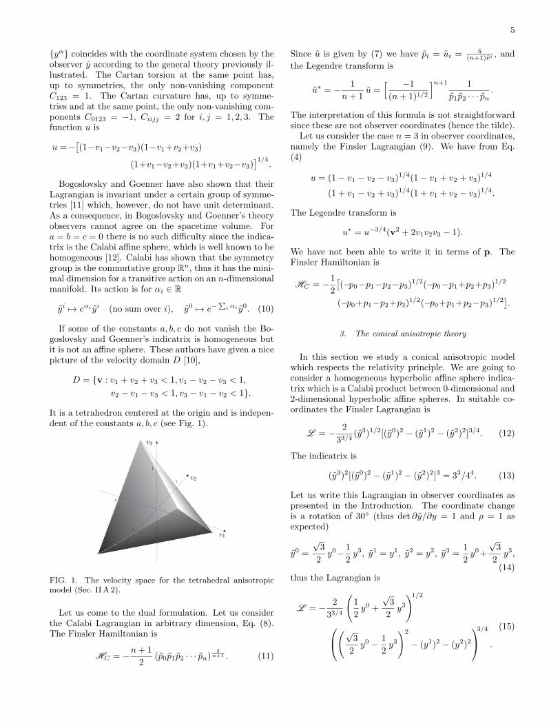
If some of the constants a, b, c do not vanish the Bo-goslovsky and Goenner’s indicatrix is homogeneous butit is not an affine sphere. These authors have given a nicepicture of the velocity domain D [10],

D = v : v1 + v2 + v3 < 1, v1 − v2 − v3 < 1,

v2 − v1 − v3 < 1, v3 − v1 − v2 < 1.

It is a tetrahedron centered at the origin and is indepen-dent of the constants a, b, c (see Fig. 1).

1

1

-1

1

-1

-1

v1

v2

v3

FIG. 1. The velocity space for the tetrahedral anisotropicmodel (Sec. II A 2).

Let us come to the dual formulation. Let us considerthe Calabi Lagrangian in arbitrary dimension, Eq. (8).The Finsler Hamiltonian is

HC = −n+ 1

2(p0p1p2 · · · pn)

2n+1 . (11)

Since u is given by (7) we have pi = ui = u(n+1)vi , and

the Legendre transform is

u∗ = − 1

n+ 1u =

[ −1

(n+ 1)1/2

]n+1 1

p1p2 · · · pn.

The interpretation of this formula is not straightforwardsince these are not observer coordinates (hence the tilde).

Let us consider the case n = 3 in observer coordinates,namely the Finsler Lagrangian (9). We have from Eq.(4)

u = (1− v1 − v2 − v3)1/4(1− v1 + v2 + v3)1/4

(1 + v1 − v2 + v3)1/4(1 + v1 + v2 − v3)1/4.

The Legendre transform is

u∗ = u−3/4(v2 + 2v1v2v3 − 1).

We have not been able to write it in terms of p. TheFinsler Hamiltonian is

HC = −1

2

[(−p0−p1−p2−p3)1/2(−p0−p1+p2+p3)1/2

(−p0+p1−p2+p3)1/2(−p0+p1+p2−p3)1/2].

3. The conical anisotropic theory

In this section we study a conical anisotropic modelwhich respects the relativity principle. We are going toconsider a homogeneous hyperbolic affine sphere indica-trix which is a Calabi product between 0-dimensional and2-dimensional hyperbolic affine spheres. In suitable co-ordinates the Finsler Lagrangian is

L = − 2

33/4(y3)1/2[(y0)2 − (y1)2 − (y2)2]3/4. (12)

The indicatrix is

(y3)2[(y0)2 − (y1)2 − (y2)2]3 = 33/44. (13)

Let us write this Lagrangian in observer coordinates aspresented in the Introduction. The coordinate changeis a rotation of 30 (thus det ∂y/∂y = 1 and ρ = 1 asexpected)

y0 =

√3

2y0− 1

2y3, y1 = y1, y2 = y2, y3 =

1

2y0+

√3

2y3,

(14)thus the Lagrangian is

L = − 2

33/4

(1

2y0 +

√3

2y3

)1/2

(√3

2y0 − 1

2y3

)2

− (y1)2 − (y2)2

3/4

.

(15)

6

The velocity domain is a circular cone with barycenter atthe origin of coordinates (see Fig. 2). Its height is equalto the diameter of the base, namely 4√

3.

D =v : v3 > −1/

√3, v3 <

√3− 2

√v2

1 + v22

. (16)

2

1

-1

-2

2

2

1

1

-2

-2

-1

-1 v1

v2

v3

FIG. 2. The velocity space for the conical anisotropic model(Sec. II A 3).

It can be checked that yα are indeed observer coor-dinates, in the sense that y = (1, 0, 0, 0) belongs to theindicatrix and at this point dL = −dy0, gαβ = ηαβ . Thefunction u is

u = − 2

33/8

(1

2+

√3

2v3

)1/4(√3

2− v3

2

)2

−(v1

)2−(v2

)23/8

While a conic velocity domain D departs very much fromthe sphericity of the isotropic case, it does so in a milderway with respect to the tetrahedral model. Also it mustbe taken into account that in most experiments only thetwo-way light speed is measured. This speed is the har-monic mean of the light speeds in opposite orientations,so as Fig. 3 shows, the anisotropic features might appearsmaller. Let us imagine a world ruled by this type of

1.0

0.5

-1.0 1.00-0.5 0.5

3/2

arctan(½)

v3

v1

FIG. 3. The two-way speed compared with the constant speed√3/2. We set v2 = 0 since there is rotational symmetry about

the third axis.

anisotropy where the 1-2 plane could be identified at any

point of the earth surface with the horizontal plane. Al-though the anisotropy of the model is considerable, sev-eral experiments would not detect it, for instance if theplane x-y can be identified with the horizontal plane thenit would be necessary to tilt the plane of a Michelson-Morley apparatus in order to detect some anisotropy.

The action of the symmetry group on the coordi-nates yα is clear. The symmetry group is a productO+(2, 1) × R where the former factor is the isochronousLorentz group while the last factor is given by the action(α ∈ R)

y3 7→ e3αy3, (y0, y1, y2) 7→ e−α(y0, y1, y2). (17)

Using the change of coordinates (14) it is easy to writethe general boost K = S−1BES, where S is the trans-formation (14) and B ×E is an element of O+(2, 1)×Rwhere B is the usual boost parametrized with a vector~β = (β1, β2) and γ := 1/

√1− β2. The matrix which

sends (y0, y1, y2, y3)> to (y′0, y′1, y′2, y′3)> is14 (3γe3α+1) −

√3

2 γβ1 −√

32 γβ2

√3

4 (1−γe−α)

−√

32 β1γe

3α (γ−1)β21

β2 +1 (γ−1)β1β2

β2β1γe

−α

2

−√

32 γβ2e

3α (γ−1)β1β2

β2

(γ−1)β22

β2 +1 γβ2e−α

2√3

4 (1−γe3α) γβ1

2γβ2

214 (γe−α+3)

From the first column we read that the unprimed ob-server moves with velocity

v1 =−2√

3β1γe3α

3γe3α+1; v2 =−2

√3β2γe

3α

3γe3α+1; v3 =

√3(1−γe3α)

3γe3α+1,

with respect to the primed observer. We can express(β1, β2, α) in terms of (v1, v2, v3) as follows

~β = −2~v√

3− v3

,

α =1

3log

√

(√

3− v3)2 − 4(v21 + v2

2)

3v3 +√

3

.

In order to obtain the velocity ξ of the primed ob-server with respect to the unprimed observer one canconsider the first column of the inverse matrix or passfrom (v1, v2, v3) to the group parameters (β1, β2, α), in-vert their signs and then calculate the correspondingvalue of the velocities. As a result

ξ3 =√

3v2

1 + v22 − v3

(v3 −

√3)

v21 + v2

2 + (2v3 +√

3)(v3 −√

3),

which shows at once that ξ 6= −v, an effect due tothe anisotropy of the space. The analysis simplifies

considerably for frames related with ~β = 0. We have

e3α =√

3−v3v+√

3, thus since α is an additive parameter, the

law of addition of velocities along the third axis is

w =u+ v + 2uv/

√3

1 + uv. (18)

7

Observe that if u = −v it is not true that w = 0. Thisfact means that boosting forward and then backward bythe same ‘velocity’ does not bring us back to the orig-inal frame. This is an anisotropic effect not present inSpecial Relativity. In order to return to the same framewe have to choose u = − v

1+2v/√

3which gives the ve-

locity of the primed observer with respect to the un-primed observer. The law of addition of velocities doesnot change if we pass from the ‘passive’ to the ‘active’velocities namely whether u, v, w represent the velocityof the boosted frame with respect to the original one orconversely, provided we stick to the same interpretationfor all the velocities.

Also observe that if u =√

3 or u = −1/√

3 then thesame holds for w irrespective of the value of v. This factis expression of the invariance of the light cone. Finally,observe that boosts along the third axis do not affect thetransversal coordinates.

Up to symmetries the non-vanishing components of theCartan torsion are

C311 = C322 =1√3, C333 = − 2√

3.

Some components of the Cartan curvature in observercoordinates can be read from the next expansion [43]

u(v) = o(|v|4)− 1 +v2

2+v3

√3

[(v1)2 + (v2)2 − 2

3(v3)2

]+

1

24

[2(

4(v3)4 +((v1)2 + (v2)2

)2)+ 3(v2)2

].

Let us consider the dual formulation. Since the FinslerLagrangian is given by (12) the Finsler Hamiltonian is

H = − 2

33/4(p3)1/2

[(p0)2 − (p1)2 − (p2)2

]3/4. (19)

In observer coordinates it reads

H = − 2

33/4

(− 1

2p0 +

√3

2p3

)1/2

((√3

2p0 +

1

2p3

)2

− (p1)2 − (p2)2)3/4

.

(20)

It does not seem possible to find a simple analytic ex-pression for the Hamiltonian u∗, nevertheless we foundthat its Taylor expansion is

u∗(p) =√

1 + p2− p3√3

[(p1)2+(p2)2− 2

3(p3)2

]+o(|p|3),

which gives the dispersion relation for this model.

Remark II.1. Bogoslovsky proposed an anisotropic La-grangian intended to depart minimally from the isotropiccase [8, 9]. Its study was then revived with the proposalof the Very Special Relativity theory [16, 20]. With arotation of the reference frame it can be brought to theform (b ∈ R is an anisotropy parameter)

LB = −1

2(y0 − y1)2b[(y0)2 − y2]1−b. (21)

Taking the determinant of the Hessian we obtain

det gαβ = (b− 1)3(1 + b)(y0 − y1)8b[(y0)2 − y2]−4b

= 16(b− 1)3(1 + b)L 4B

[(y0)2 − y2]4,

which shows that whenever g is non-degenerate it mustbe |b| 6= 1 and the determinant depends on y. The meanCartan torsion does not vanish thus, it is not an affinesphere. According to our previous discussion the indica-trix is not transitively preserved by a group of unimod-ular linear transformations, and so it does not respectthe relativity principle as we defined it. This model forb = 1/4 should not be confused with that given by Eq.(12). See [37, 61] for a discussion of the symmetries ofthe two factors.

III. THE GENERAL THEORY

In this section we consider the four-dimensional affinesphere spacetimes which satisfy the relativity principle atevery point. This means that at TxM the geometry of theindicatrix belongs to one of the three types studied in theprevious sections, with the difference that now L (x, y)might indeed depend on x.

The solution of this problem is in fact very simple andconsists in introducing over each coordinate chart on M ,a basis of one-forms ea = eaµ(x)dxµ, a = 0, 1, 2, 3, called

vierbeins such that µ = |e0 ∧ e1 ∧ e2 ∧ e3| is the space-time volume form. They provide an isomorphism be-tween TxM and a model Lorentz-Minkowski space pro-vided we assume that det e 6= 0. Then the isotropic,tetrahedral anisotropic, and conical anisotropic modelsread respectively:

L =1

2

(− (e0

σ(x)yσ)2 + (e1σ(x)yσ)2

+ (e2σ(x)yσ)2 + (e3

σ(x)yσ)2),

(22)

L = −2[Π4a=0(eaσ(x)yσ)

]1/2, (23)

L = − 2

33/4(e3µ(x)yµ)1/2

[(e0γ(x)yγ)2 −(e1

α(x)yα)2

−(e2β(x)yβ)2

]3/4.

(24)

It is indeed clear that on each tangent space TxM weobtain the anisotropic theories studied in the previoussection.

A. Kinematical reformulation

The established isomorphism between TxM and themodel Lorentz-Minkowski space is largely arbitrarywhenever the latter admits a symmetry group. As a con-sequence, it can be convenient to replace the vierbeinvariable with less arbitrary objects.

8

Introduced the metric gαβ(x) = ηab eaα(x) ebβ(x) the

isotropic model becomes

L =1

2gαβ(x) yαyβ , µ =

√|det gαβ |d4x,

namely the isotropic theory depends only on a Lo-rentzian metric.

The tetrahedral anisotropic theory cannot be fur-ther simplified in the sense that one has to workwith four one-forms. These forms are not com-pletely arbitrary since det e 6= 0.

Concerning the conical anisotropic theory, let tµ :=e3µ, and let ξhαβ(x) := ηab e

aα(x) ebβ(x) where ηab =

ηab for a, b 6= 3 and zero otherwise. Evidently ξhis a degenerate metric of signature (−,+,+, 0). Itskernel is spanned by a vector ξ such that e3(ξ) = 1,e0(ξ) = e1(ξ) = e2(ξ) = 0, thus tµξ

µ = 1. Our no-tation ξh is meant to remind us that ξh is degener-ate with kernel spanned by ξ. Recalling the general-ized Cauchy-Binet formula for the minors of a prod-uct of matrices, Mαβ(AB) =

∑γMαγ(A)Mγβ(B),

we obtain

Mαβ(ξh) = −M3α(e)M3β(e).

Moreover, using the Laplace expansion for the de-terminant, and selecting the last row to calculatethe expansion

det e =∑µ

(−1)µtµM3µ(e),

thus (det e)2 = −(−1)α+βMαβ(ξh)tαtβ . This iden-tity can be suggestively written

(det e)2 = (− det ξh)ξhαβtαtβ ,

where it is understood that this expression is justa mnemonic aid to recover the above expressioninvolving minors. Indeed, ξh cannot be really in-verted since it is degenerate. Finally, this theory isreduced to the Lagrangian and associated volumeform

L = − 2

33/4

(tµ(x)yµ

)1/2(ξhαβ(x) yαyβ)3/4,

µ =√|det ξh| |ξhαβtαtβ |d4x.

where the square root appearing in the volume formis positive and ξh has signature (−,+,+, 0).

The comparison of the theory with observation mightrequire a different choice of vierbeins

eaµ = Mabebµ,

where M is the matrix which in the previous section ac-complished the change of coordinates ya = Ma

byb (thus

Mab = δab in the isotropic theory, while M is just a rota-

tion of 30 degrees in the 0-3 plane in the conic theory). Infact, whenever eiµy

µ e0µy

µ (e.g. because e00 > 0, ei0 = 0

and yj y0) we have that the Lagrangian of the tetra-hedral or conic theories is approximated by the isotropicone. In other words, in that velocity limit the Finsleriankinematics reduces itself to the general relativistic one.

B. Dynamics

This section shows how to construct a dynamical La-grangian or the field equations for the kinematical mod-els. It can be skipped on first reading.

In order to define a dynamics we shall need an ac-tion. Fortunately, due to the affine sphere condition wehave already a well defined volume form on M so weneed only to define a scalar Lagrangian. The traditionalapproach in Finsler gravity theory consists in trying tobuild, if not a Lagrangian, some field equations directlyfrom the various curvatures associated to the Berwald,Cartan or Chern-Rund Finsler connections. This ap-proach has been followed by Horvath [23], Takano [58],Ishikawa [25, 26], Ikeda [24], Asanov [2], Miron [45], Rutz[54], Li and Chang [33], Vacaru [59], Pfeifer and Wohl-farth [49], to mention a few. The author has also ex-plored this route [38]. It has the drawback that the soobtained equations would depend on the fiber variables,a fact which complicates their interpretation as evolutionequations.

Here we are going to construct dynamical equationswhich do not depend on the fiber variables and which,variationally speaking, do not introduce complicationsrelated to the integration over the non-compact indica-trix. We do not use the Finslerian curvatures but rather,construct a gauge theory from the fields which enter thedefinition of Finsler Lagrangian. The number and natureof these fields depend on the model considered.

In fact, the most straightforward approach towards thedynamics of the theory consists in gauging the interiorsymmetry. This gauging is necessary since the FinslerLagrangian is largely independent of the vierbein choiceand so should be the dynamics. As we mentioned, the in-terior groups of vierbein transformations which leave theFinsler Lagrangians (22)-(24) invariant are O+(3, 1), R3

and O+(2, 1)×R, respectively. We assume the existenceof a G-structure over M , where G is the interior group.This hypothesis allows us to assume the existence of ag-valued connection and hence of a g-valued curvature.

In the isotropic case we have a natural gauge in-variant object, namely the spacetime metric gµν :=ηabe

aµebν . Thus a gauge invariant Lagrangian can be

obtained from a scalar constructed from the met-ric. Of course, general relativity tells us that theappropriate scalar is the Ricci scalar.

We have four 1-form variables eaµ, a = 0, 1, 2, 3, and

three 1-form Abelian connections Aiµ, i = 1, 2, 3,

9

due to the three Abelian gauge symmetries c.f. Eq.(10), A′iµ = Aiµ − ∂µαi

e′0ν = e−∑i αi e0

ν , (25)

e′iν = eαi eiν , (26)

where e0 has charge (q1, q2, q3) = (−1,−1,−1), e1

has charge (1, 0, 0), e2 has charge (0, 1, 0) and e3 hascharge (0, 0, 1). We introduce a covariant derivativewhich takes into account these charges

Dµe0ν = ∂µe

0ν − (

∑i

Aiµ)e0ν ,

Dµeiν = ∂µe

iν +Aiµe

iν , i = 1, 2, 3.

These covariant derivatives are left invariant underthe gauge transformation. The vierbeins eνa haveopposite charges so that an upper interior indexbrings the opposite charge of a lower interior indexand the interior contractions are uncharged.

Observe that we have four linearly independent1-forms which can be arbitrarily rescaled thoughgauge transformations provided the volume form isleft invariant. Dually, we have four linearly inde-pendent vectors which can be arbitrarily rescaledprovided their wedge product is left invariant.These vierbeins determine at each point four pre-ferred directions but no preferred scale along thosedirections. It is a kind of geometry slightly morerelaxed than Weitzenbock’s. There the connectionwould be obtained imposing the parallel translationof the vierbein field ∇Wα eaµ = ∂αe

aµ − ΓWσ

µαeaσ = 0,

thus ΓWσµα = eσa∂αe

aµ, while here we have to replace

ordinary derivatives with gauge derivatives thus

∇αeaµ = Dαeaµ−Γσµαe

aσ = 0, ⇒ Γσµα = eσaDαe

aµ.

The connection coefficients Γ determine a linearconnection ∇ from which we can construct the tor-sion tensor

Tαµν = Γανµ − Γαµν = eαaDµeaν − eαaDν e

aµ

and the curvature Rαβγδ. Thus, introducing the

Abelian curvatures F iµν = ∂µAiν − ∂νAiµ, the most

general action for this theory is

S =

∫f(R, T, F, e) det(eaµ)dx,

where with e we mean the vierbeins or their dual.It should be observed that contrary to the isotropictheory we do not have an interior metric ηab whichthrough gµν = eµaη

abeνb could allow us to contractlower spacetime indices. Furthermore, R, T , F arepredominant in the lower indices so the construc-tion of a scalar appears non-trivial. Some interest-ing scalars are

|det(R(αβ))|1/2

det(eaν),

Pf(F iαβ)

det(eaν),

where R(αβ) is the symmetrized Ricci tensor andPf is the Pfaffian. The latter choice gives an actionterm of topological origin while the former choiceis inspired by Eddington’s purely affine action [50].If Bαβ denotes the transpose of the cofactor matrixof R(αβ), namely the matrix such that BαβR(βγ) =det(R(αβ))δ

αγ , then particularly interesting is the

action∫ (|det(R(αβ))|1/2+

∑i

ciFiαβF

iγδ

BαγBβδ

[det(eaα)]3

)d4x,

where ci are coupling constants.

Some other possibilities are offered by the tenso-riality of the following uncharged object tαβγδ :=

eα0 eβ1 eγ2 eδ3. Then other examples of scalars which

might enter the construction of a Lagrangian are

RαβRγδtαβγδ, F iαβF

iγδt

αβγδ, RαβFiγδt

αβγδ,

or various combinations in the fourth power of thetorsion e.g.

TαβγTγναT

δηρT

ρµδt

βνηµ.

Finally, there is the possibility of writing directlyfield equations of non-variational origin by equatingequally charged terms.

In the conic theory the O+(2, 1)-gauge invariancecan be accomplished constructing the Lagrangianfrom the O+(2, 1)-gauge invariant fields tµ andξhαβ . Additionally, we have a gauge field Aµ dueto the Abelian gauge symmetry cf. Eq. (17)

A′µ = Aµ − ∂µα, (27)

t′µ = e3αtµ, (28)

ξh′µν = e−α ξhµν , (29)

namely t has charge 3 while ξh has charge −1. Thevector ξ has change −3.

The pair (tµ,ξhαβ), where ξ spans the kernel of ξhαβ

and tµξµ = 1, can be easily shown to be equiva-

lent to a triple (tµ, hαβ , ξν), where hαβ is a con-

travariant metric of nullity one, hαβtβ = 0, andξhαβ := hαµ ξhµβ = δαβ−ξαtβ is the projector on ker t

determined by the spitting TxM = (ker t⊕ 〈ξ〉)|x.

The tensor hαβ does not bring the ξ label because itis, in a well defined sense, independent of it. In fact,it really depends only on ξhαβ |ker t. This metric isnon-degenerate thus it has an inverse (ξh|ker t)

−1

which acts as a bilinear form on ker t∗. But anyelement of ker t∗ can be regarded as an equivalenceclass of forms, any two forms being equivalent ifthey differ by a term proportional to t. As a conse-quence (ξhαβ |ker t)

−1 can be represented by a con-travariant metric which annihilates tβ , this is hαβ .

10

Observe that hαβ has charge 1. The reader ac-quainted with the geometrical formulation of theNewtonian gravitational theory will recognize itsmain geometric ingredients [30, 35] with three rele-vant differences (a) the metrics hαβ and ξhαβ havesignature (−,+,+, 0) rather than (+,+,+, 0), (b)the fields are charged, (c) the dynamics depends ona ‘non-relativistic matter’ field ξ.

Let us construct a dynamics which is reminiscentof Newtonian gravity. We introduce a derivativewhich takes into account the charges

Dµtν = ∂µtν + 3Aµtν ,

Dµhαβ = ∂µh

αβ +Aµhαβ ,

Dµξν = ∂µξ

ν − 3Aµξν .

Next we introduce an affine connection ∇ throughits coefficients Γαµν and impose that the fields(tα, h

µν) be covariantly constant with respect tothe gauged covariant derivative

∇µtν = ∇µtν+3Aµtν = Dµtν −Γανµtα = 0, (30)

∇µhαβ = ∇µhαβ +Aµhαβ

= Dµhαβ+Γασµh

σβ+Γβσµhασ = 0.

(31)

The former equation implies that the torsion Tαµν :=Γανµ − Γαµν satisfies

Tαµνtα = (dt+ 3A ∧ t)µν = 0,

thus the connection is torsionless only if ker t is inte-grable. We shall assume that the connection is tor-sionless. Defined the curvature Fµν = ∂µAν−∂νAµ,the previous equations imply F ∧ t = 0, namely the‘magnetic’ components vanish and so F is purely‘electric’.

Observe that the light cone includes a distinguishedflat boundary which provides us with a distributionof hyperplanes ker t over the manifold. Since thedistribution is integrable we have a natural folia-tion which can be interpreted as a global absolutenotion of simultaneity. Over each slice we have aLorentzian metric, thus the spacetime M is foli-ated by a one-parameter family of Lorentzian man-ifolds. Given a curve x : I → M , s → x(s), such

that tµdxµ

ds > 0 (i.e. classically timelike) the integral∫tµ

dxµ

ds ds cannot represent the time of the particlesince tµ is not gauge invariant. This is an impor-tant difference with respect to the Newtonian the-ory. The meaningful proper time over the trajec-tory is that calculated via the Finsler Lagrangian:∫ √−2L (x, x′)ds. Curiously, as we shall clarify in

a moment, the conic theory mingles a sort of for-mally non-relativistic field dynamics together witha relativistic notion of proper time.

Let us raise indices with hαβ . As in Newton-Cartantheory [18, 30] we consider connections of the form

(observe that we took into account the Abeliangauge symmetry)

Γµαβ = hµσ1

2

(Dβ

ξhασ +Dαξhσβ−Dσ

ξhαβ)

+D(αtβ)ξµ + t(αΩβ)σh

σµ.

where Ωαβ = −2 ξhγ[α ∇β]ξγ vanishes if and only

if ξ is geodesic and twist-free, ξµ ∇µξν = 0,

∇[µξν] = 0. Observe that the connection is un-charged.

Mimicking Newton-Cartan theory, the vacuum dy-namics for hαβ and Aµ can be assigned to be

Rαβ = 0, ∇βFαβ = 0. (32)

The vector field ξ could be assigned a dynamics for-mally analogous to that of a non-relativistic fluid.

Of course, completely different dynamics couldhave been considered, e.g. in those cases in which Γhas torsion. In fact, many scalars can be built fromthe torsion and curvature of Γ. In order to contractlower indices one could use the tensoriality of theobject

(det ξh)ξhµν/[|det ξh| |ξhαβtαtβ |].

These considerations were aimed at illustrating thepossibility of defining a dynamics for the Finslerian kine-matical theories previously introduced. In the next sec-tion we shall show that it is not necessary to impose somedynamical equations and to solve them in order to selectphysically interesting affine sphere spacetimes. Indeed,these spaces will be uniquely selected from the imposi-tion of an appropriate general relativistic limit. Thesenotable spacetimes might then help to select the correctfield equations.

C. Notable affine sphere spacetimes

We can construct some first examples of general rel-ativistic affine sphere spacetimes which satisfy the rela-tivity principle. We shall impose that at every point thespacetime is conic anisotropic obtaining conic anisotropicgeneralizations of the Kerr-Schild, Schwarzschild, Kerr,Taub, FLRW metrics. A test particle slowly moving onthese spacetimes with respect to their natural stationaryobserver would behave as in the corresponding Loren-tzian spacetimes of general relativity. I have not beenable to obtain similarly good results for the tetrahedraltheory.

D. Conic anisotropic generalization of theKerr-Schild metric

We recall that the fiber coordinate is defined by yµ =dxµ : TxM → Rn+1. In this section we might revert to

11

the notation dxµ for the fiber coordinate. Let f : U → R,µ : U → (0, 2π)\π/2, π, 3π/2, U ⊂M , be functions andlet k = kαdxα = dt + kxdx + kydy + kzdz be a 1-formfield on the same coordinate patch U . Let us define

β =√

(1− f) + fk2z ,

ω⊥ = kxdx+ kydy,

ωt = dt− f

1− f(kxdx+ kydy + kzdz),

ωz =1

β

(dz +

f

1− fkz(kxdx+ kydy + kzdz)

).

Let us consider the Finsler Lagrangian

L = − 1− f2(cos2µ)cos2µ(sin2µ)sin2µ

((sinµωt+cosµωz)

2)sin2µ

((cosµωt−sinµωz)

2− 1

1−f

(dx2+dy2+

f

β2ω2⊥

))cos2µ

(33)

This expression is left invariant if we change the orienta-tion of z, x with y, and the sign of sinµ, thus µ can beassumed in the range (0, π) with no loss of generality.

Its limit for large distances (large max(|xi|)) is

L∞ = − 1

2(cos2µ)cos2µ(sin2µ)sin2µ

((sin µdt+cos µdz)

2)sin2µ

((cos µdt−sin µdz)

2−dx2−dy2)cos2µ

, (34)

provided for every α, β, we have fkαkβ → 0 and µ → µin that limit.

If µ = µ is a constant throughoutM then L is modeledon the same Lorentz-Minkowski space L∞ at every point.

At every point x ∈M the vector y = ( 1√1−f , 0, 0, 0) be-

longs to the indicatrix and so provides an observer vectorfield which will be of particular interest whenever (M,L )is stationary, that is, independent of time.

For low velocities with respect to y, yi y0, and forevery function µ(x), the Lagrangian reduces itself to theKerr-Schild metric

ds2 = −dt2 + dx2 + dy2 + dz2 + fkαkβdxαdxβ .

Under the assumption fkαkβ → 0 it is asymptotic to theMinkowski metric which is indeed the low velocity limitof L∞.

For µ = π/6 namely with

L = −2(1− f)

33/4

(1

2ωt +

√3

2ωz

)21/4

(35)

(√3

2ωt−

1

2ωz

)2

− 1

1−f

(dx2 + dy2+

f

β2ω2⊥

)3/4the indicatrix is a Calabi product of affine spheres, thusit is itself an affine sphere and hence its mean Cartantorsion vanishes. Its asymptotic limit and model Lorentz-Minkowski space is

L∞ = − 2

33/4

(1

2dt+

√3

2dz

)21/4

(√3

2dt− 1

2dz

)2

− dx2 − dy2

3/4(36)

If µ is different from this special value the mean Car-tan torsion does not vanish. Indeed, a calculation at theobserver y gives

Iα(y) =2(3− 4 cos2µ)

β√

1−f cosµ sinµ

(0, fk1k3, fk2k3, β

2). (37)

Now, for any chosen µ(x) we can obtain from (33) theFinslerian conic anisotropic version of many general rela-tivistic metrics. For instance, for the Kerr-Newman met-ric in Kerr-Schild Cartesian coordinates [22] we set forsome constants m > 0, a, q

kα =(1,rx+ ay

a2 + r2,ry − axa2 + r2

,z

r

),

f =2mr3 − q2r2

a2z2 + r4,

where r(x, y, z) is determined implicitly, up to a sign, bythe requirement that k be null, namely

x2 + y2

a2 + r2+z2

r2= 1.

Similarly, the Kerr-de Sitter metric can be obtained fromk and r as above with a = 0, by setting

f =2m

r+

Λ

3r2.

For the Schwarzschild metric (a = Λ = 0) it can beconvenient to introduce cylindrical coordinates (z, ρ, ϕ),pass to the Schwarzschild time tS through

t = tS + 2m ln | r2m− 1|,

in such a way that ωt = dtS , set r =√z2 + ρ2 and set

for definiteness µ = π/6, then

12

L = −2(1− 2m

r )

33/4

(1

2dtS +

√3

2

(1− 2m

r

)−1(1− 2mρ2/r3)dz + 2mzρdρ√

1− 2mρ2/r3

)21/4

(√3

2dtS−

1

2

(1− 2m

r

)−1(1−2mρ2/r3)dz + 2mzρdρ√

1− 2mρ2/r3

)2

−(

1− 2m

r

)−1(dρ2

1− 2mρ2/r3+ ρ2dϕ2

)3/4

.

(38)

The metric can be written using Boyer-Linquist coor-dinates (r, θ, ϕ) defined by

x+ iy = (r + ia) sin θ exp i

(ϕ+ a

∫dr

r2 − 2mr + a2

),

z = r cos θ, t = t+ 2m

∫rdr

r2 − 2mr + a2,

by noticing that

ω⊥ =(r2 − 2mr) sin2 θ

r2 − 2mr + a2dr + r sin θ cos θdθ

− a sin2 θdϕ,

ω +zdz

r=

(1− a2 sin2 θ

r2 − 2mr + a2

)dr − a sin2 θdϕ,

dx2 + dy2 =r2 sin2(θ)

(a2 + (r − 2m)2

)(r2 − 2mr + a2)

2 dr2

+ (r2 + a2) sin2 θdϕ2 + (r2 + a2) cos2 θdθ2

+4amr sin2 θ

r2 − 2mr + a2drdϕ+ 2r cos θ sin θdrdθ.

The final expression is not particularly illuminating, how-ever, it shows that the Finsler Lagrangian has Killingvectors ∂t, ∂φ. We have

α = 1− 2mr

r2 + a2 cos2 θ,

β =

√1− 2m sin2 θ

r,

ω⊥ =(r2 − 2mr) sin2 θ

r2 − 2mr + a2dr + r sin θ cos θdθ

− a sin2 θdϕ,

ωt = dt+2mr sin2 θ

r2 − 2mr + a2 cos2 θadϕ,

ωz =1

β

(a2 + r2)

cos θ

r2 − 2mr + a2dr − r sin θdθ

− 2mr cos θ sin2 θ

r2 − 2mr + a2 cos2 θadϕ

,

dx2 + dy2 = sin2 θdr2 + r2 sin2 θdφ2 + r2 cos2 θdθ2

+ 2r cos θ sin θdrdθ.

The Finsler Lagrangian becomes

L = − 2α

33/4

(1

2ωt +

√3

2ωz

)1/2

(39)

(√3

2ωt −

1

2ωz

)2

− 1

α

(dx2 + dy2 +

2m

rβ2ω2⊥

)3/4

The low velocity limit gives the Kerr metric in Boyer-Linquist coordinates. For a = 0, ωt = dt, the low veloc-ity metric is Schwarzschild’s and t is the Schwarzschild’stime.

E. A cosmological model

In this section we shall construct the conic anisotropicversions of the FLRW metrics with k = 1 or k = 0. Weshall also obtain the conic anisotropic version of the Taubsolution. For k = 1 the idea is to regard the S3 spacesection as a Hopf fibration and to orient the anisotropicdirection of the conic anisotropy along the Clifford par-allels, that is, along the fibers.

1. The Hopf bundle

Let us first recall the construction of the Hopf fibration.This introduction will also serve to fix the notation. Letan element of SU(2) be parametrized as follows

w =

(z0 −z1

z1 z0

), |z0|2 + |z1|2 = 1.

This expression clarifies that SU(2) is diffeomorphic toS3. Let us denote with σi the Pauli matrices

σ1 =

(0 11 0

), σ2 =

(0 −ii 0

), σ3 =

(1 00 −1

),

and let τk = iσk/2 be the generators of the Lie algebrasu(2),

[τi, τj ] = εijkτk.

Every element of SU(2) is also a linear combination ofthe identity and τk. It will be useful to recall the identity

σiσj = iεijkσk + δij I,

13

and that detσi = −1. Let us define the map over SU(2)

π(w) = 2wτ3w†,

some algebra shows that

π(w) = 2wτ3w† = i

(a bb −a

)=

(ia −ibib ia

),

where a = |z0|2 − |z1|2 ∈ R, and b = 2z1z0 ∈ C. Observethat π(w) belongs to SU(2) ∩ su(2) thus detπ(w) = 1which reads a2 + |b|2 = 1. We conclude that π(w) ∈ S2.

The group SU(2) admits a subgroup isomorphic toU(1) given by the matrices of the form

ρ(ϕ) =

(eiϕ 00 e−iϕ

),

which is generated by τ3. Its right action on SU(2) canbe defined through

U(1)× SU(2)→ SU(2),

(w, ρ(ϕ)) 7→ wρ(ϕ).

Since ρ(ϕ) commutes with τ3

π(wρ(ϕ)) = 2wρ(ϕ)τ3ρ(ϕ)−1w−1 = 2wτ3w−1 = π(w).

Thus the projection π : S3 → S2 has fiber S1. This isthe Hopf fiber bundle. Let u ∈ S2, namely let u be amatrix of the form 2wτ3w

† for w ∈ SU(2), if h ∈ SU(2),huh−1 = π(hw) ∈ S2 thus SU(2) acts on S2 as a trans-formation induced from a linear transformation of R3.We shall see later that this is an isometry, so that SU(2)acts as a rotation. This is the double covering of SU(2)over SO(3).

2. Metrics over the Hopf bundle

The idea is to construct the cone of the Finsler La-grangian as the product between a one dimensional coneand a three dimensional irreducible cone, or equivalentlythe indicatrix should be the Calabi product between azero dimensional affine sphere and an irreducible two di-mensional affine sphere. We are going to construct thethree dimensional cone from a Lorentzian metric on theHopf fiber bundle. We wish to avoid coordinates as far aspossible so as to make the presentation clearer. Coordi-nates will be introduced in the end. The (left-invariant)Maurer-Cartan form of SU(2) is

θ = w†dw =

(z0dz0 + z1dz1 −z0dz1 + z1dz0

−z1dz0 + z0dz1 z1dz1 + z0dz0

)It can be observed that since |z0|2 + |z1|2 = 1 we havetr θ = 0. It can be interesting to observe that for an arbi-trary 2×2 matrix M (this formula admits generalizationto higher dimensions)

detM =1

2det

(trM 1trM2 trM

)=

1

2

((trM)2 − trM2

),

thus

−1

2tr(θ2) =

1

2tr(dw†dw) = det(θ)

= dz0dz0 + dz1dz1 = gS3 . (40)

This is precisely the metric induced on S3 by the Eu-clidean metric in R4 (decompose z0 and z1 in real andimaginary components).

Similarly, the metric induced on S2 by the Euclideanmetric of R3 is

−1

2tr((π(w)†dπ(w))2

)= d(ia)d(ia) + d(ib)d(ib)

= da2 + dbdb = gS2 .(41)

Since θ is su(2)-valued we decompose it as followsθ = τkωk where ωk are real 1-forms over SU(2). Usingtr(σiσj) = 2δij or tr(τiτj) = − 1

2δij we get

ωk = −2tr(θτk).

This expression shows at once that ω3 is invariant underthe right action of U(1), indeed let us calculate R∗aω3 witha ∈ SU(2), (observe that R∗aθ = (wa)†d(wa) = a†θa)

R∗aω3(X) = −2tr(θ(Ra∗X))τ3) = −2tr((R∗aθ)(X))τ3)

= −2tr(a−1θ(X)aτ3),

so since ρ(ϕ) commutes with τ3, R∗ρ(ϕ)ω3 = ω3. The

1-form ω3 is actually a connection for the Hopf bundle.Indeed, the vertical fundamental field is τ∗3 , and by def-inition of θ, θ(τ∗3 ) = τ3, thus ω3(τ∗3 ) = −2tr(τ3τ3) = 1(see [28] for the conditions defining a connection on aprincipal bundle).

There is also a U(1)-invariant metric, indeed,

ω21 +ω2

2 = (ω21 +ω2

2 +ω23)−ω2

3 = −2tr(θ2)− (2tr(θτ3))2.

The validity of this equation can be checked insertingθ = ωkτk and using again tr(τiτj) = − 1

2δij . Arguing as

above R∗ρ(ϕ)(ω21 + ω2

2) = ω21 + ω2

2 .

As the next trace vanishes

tr(π(w)†dπ(w)

)= 4tr

[wτ3w

†(wτ3(−w†dww†)+dwτ3w†)]

= tr(dww†)− tr(w†dw) = 0.

we can write

−1

2tr((π(w)†dπ(w))2

)= det(π(w)†dπ(w)) = det

(dπ(w)

)= 4 det(dwτ3w

† − wτ3w†dww†)= 4 det(w†dwτ3 − τ3w†dw) = 4 det([θ, τ3])

= 4 det(−ω1τ2 + ω2τ1) = ω21 + ω2

2 .

This result jointly with Eq. (41) shows that ω21 + ω2

2 isthe (π-pullback of the) canonical metric of S2. Observethat the action of SU(2) on S2, π(w) 7→ hπ(w)h−1 is anisometry for this metric which proves the earlier state-ment that SU(2) is a double covering of SO(3) (h and−h give the same map).

14

Remark III.1. If one insists on using coordinates it isconvenient to parametrize SU(2) as follows

w(φ, θ, ψ) =

(ei2 (ψ−φ) cos(θ/2) −e− i

2 (ψ+φ) sin(θ/2)

ei2 (ψ+φ) sin(θ/2) e−

i2 (ψ−φ) cos(θ/2)

),

that is

z0 = ei2 (ψ−φ) cos(θ/2), z1 = e

i2 (ψ+φ) sin(θ/2),

with φ ∈ [0, 2π), ψ ∈ [0, 4π), θ ∈ [0, π] (the angle ψ canbe given the domain [0, 2π) if one is interested in generat-ing the SO(3) group through the action x′iσi = wxiσiw

†,however in order to generate SU(2) one needs to doublethe domain of ψ in order to generate the negated matri-ces.

This parametrization is particularly useful because

π(w(φ, θ, ψ)) = iwσ3w† = inkσk

with n1 = sin θ cosφ, n2 = sin θ sinφ, n3 = cos θ. Theinvariants under U(1)-right translations are

ω3 = dψ − cos θdφ,

ω21 + ω2

2 = dθ2 + sin2 θdφ2.

The other 1-forms are

ω1 =sinψdθ+cosψ sin θdφ; ω2 =− cosψdθ+sin θ sinψdφ.

Any metric over S3 of the form hijωiωj , where hij areconstant coefficients, is necessarily invariant under theleft SU(2) action as the forms ωi are. There are Rieman-nian metrics over S3 which share additional symmetries.For instance from Eq. (40) the metric

ω21 + ω2

2 + ω23 = −2tr(θ2) = 4gS3

= (dψ − cos θdφ)2 + dθ2 + sin2 θdφ2

is invariant under the right SU(2) action. This meansthat the isotropy group at a point, namely the subgroupwhich leaves a point fixed, is three dimensional a factwhich implies that this space is isotropic.

In order to construct the mentioned product of coneswe need a Lorentzian metric over S3. We are interestedin Lorentzian metrics over SU(2) of the form

g = −α23ω

23 + α2

⊥(ω21 + ω2

2) (42)

The forms ω3 and ω21 +ω2

2 entering this metric are invari-ant under the SU(2) left action and the U(1) right ac-tion. The metric g shares similar symmetries dependingon the functions α3 and α⊥. For instance, it respects thefull symmetry if they are constant while it respects theU(1) symmetry for α3, α⊥ : S2 → R. We are interestedin the former case for it admits an additional τ3 right-rotation which tells us that the isometry subgroup whichleaves a point fixed is non-trivial (not just the identity)and so that there is isotropy at least under rotations with

respect to some direction. This is the direction towardswhich we orient the cone domain of the conic anisotropy.

A pointwise Calabi product and the requirement ofpreservation of symmetry lead us to the next affine spherespacetime

L = − 2

33/4

(1

2α0dt+

√3

2α3ω3

)21/4

(√3

2α0dt− 1

2α3ω3

)2

−α2⊥(ω2

1 + ω22)

3/4(43)

where α3, α0, α⊥ depend on t. Observe that the U(1)right translations and the SU(2) left translations actingon the space sections S3 are symmetries for this FinslerLagrangian. It can share additional symmetries for par-ticular choices of α3, α0, α⊥. For instance, if they areconstant there is an additional R factor due to the timetranslations.

For low velocities it becomes

ds2 = −α20dt2 + α2

3ω23 + α2

⊥(ω2

1 + ω22

),

which for constants m, ` > 0, once we set

α20 = U−1, U(t) :=

`2 − 2mt+ t2

t2 + `2,

α2⊥ = t2 + `2,

α23 = 4`2U,

gives the Taub vacuum. For α3 = α⊥ = a(t)/2, α0 = 1,it gives the FLRW metric with k = 1

ds2 = −dt2 + a2(t)gS3 . (44)

Clearly, the FLRW metric with k = 0 can be obtained asthe low velocity limit of the Finsler Lagrangian

L = − 2

33/4

(1

2dt+

√3

2a(t)dz

)21/4

(45)

(√3

2dt− 1

2a(t)dz

)2

− a2(t)(dx2 + dy2)

3/4

however, there seems to be no natural conic Finsleriangeneralization of the FLRW metric with k = −1.

Remark III.2. It can be observed that while the FLRWLagrangian for k = 1, Eq. (43), has invariance groupU(1) × SU(2), its low velocity limit, Eq. (44), has moresymmetries, as it has six Killings. This fact has to beexpected on the following ground. In general, the FinslerLagrangian captures also the kinematics of light whichcould be highly anisotropic, still in the low velocitylimit one has that the indicatrix is approximated by ahyperboloid, which is isotropic. As a consequence, one

15

does not see the anisotropy of velocity space but onlythat of spacetime and so gets more symmetries (unlessthe Finslerian spacetime is obtained aligning the velocityspace anisotropy with that already present in its generalrelativistic limit as in the Kerr example). The samephenomenon can be seen with Eq. (15) which has aneight dimensional group of symmetries while the limitfor low velocities is Minkowski spacetime which has tenKillings.

IV. CONCLUSIONS

In this work we have recognized that the relativityprinciple is expressed by the homogeneity of the observerspace (indicatrix), meaning by this its transitivity underthe action of a unimodular linear group acting on thetangent space. We have also pointed out that in fourspacetime dimensions there are only three theories whichrespect an exact form of the relativity principle, the ve-locity domain of massive particles as seen from a localobserver being given by a ball, a tetrahedron or a cone,respectively. We have studied their kinematics, partic-ularly that of the conic theory since it was not previ-ously recognized. For each of these theories we have pro-vided observer coordinates, namely special coordinatesfor which the metric becomes Minkowskian in the appro-priate velocity limit.

In Sec. III we have discussed the dynamics showinghow to build consistent field equations by gauging theinterior symmetries. We did not focus on particular dy-

namical laws. Instead, we observed that notable Fins-lerian spacetimes could be selected by two requirements(a) the spacetime is relativistic invariant (the indicatrix ishomogeneous), (b) the low velocity limit with respect toa natural (conformal) stationary observer returns somenotable general relativistic metric. Using this approachwe have been able to obtain the conic anisotropic ver-sion of the Kerr-Schild metric and through it the conicanisotropic versions of the Schwarzschild, Kerr-de Sitterand Kerr-Newman spacetimes. The generalization of theFLRW metric required a preliminary study of the Hopfbundle, but in the end we obtained the conic anisotropicversions for k = 0, 1, and as a bonus we obtained also theconic anisotropic version of Taub’s spacetime.

Our study shows that other and different general rela-tivistic theories are possible. In fact some theories mightpresent curious hybrid features, namely the gravitationalfields might admit a sort of formally non-relativistic de-scription while test particles might exhibit typical rela-tivistic features, such as time dilation.

The found geometries could possibly describe peculiargravitational regions of the Universe. For our spacetimeneighborhood a perturbative approach seems more ap-propriate since the local light cones are expected to de-part slightly from isotropy. Approaches which try to re-tain an almost general relativistic dynamics while mod-ifying the indicatrix in a neighborhood of a (stationary)observer should pass through a study of modified dis-persion relations at the lowest order of approximation[21, 29, 53]. A perturbative study respecting the geome-try of affine spheres will be presented in future work.

[1] G. Amelino-Camelia, L. Barcaroli, G. Gubitosi,S. Liberati, and N. Loret. Realization of doubly spe-cial relativistic symmetries in finsler geometries. Phys.Rev. D, 90:125030, 2014.

[2] G. S. Asanov. Finsler geometry, relativity and gauge the-ories. D. Reidel Publishing Co., Dordrecht, 1985.

[3] G. S. Asanov. Finslerian extension of Schwarzschild met-ric. Fortschr. Phys., 40:667–693, 1992.

[4] V. Balan, G. Yu. Bogoslovsky, S. S. Kokarev, D. G.Pavlov, S. V. Siparov, and N. Voicu. Geometrical mod-els of the locally anisotropic space time. J. Mod. Phys.,3:1314–1335, 2012.

[5] V. Balan and S. Lebedev. On the Legendre transformand Hamiltonian formalism in Berwald-Moor geometry.Differ. Geom. Dyn. Syst., 12:4–11, 2010.

[6] S. Basilakos, A. P. Kouretsis, E. N. Saridakis, andP. C. Stavrinos. Resembling dark energy and modifiedgravity with Finsler-Randers cosmology. Phys. Rev. D,88:123510, 2013.

[7] L. Berwald. Uber Finslersche und Cartansche GeometrieII. Invarianten bei der Variation vielfacher Integrale undParallelhyperflachen in Cartanschen Raumen. Composi-tio Math., 7:141–176, 1939.

[8] G. Yu. Bogoslovsky. A special-relativistic theory of the

locally anisotropic space-time. I: The metric and groupof motions of the anisotropie space of events. Il NuovoCimento, 40 B:99–115, 1977.

[9] G. Yu. Bogoslovsky. A viable model of locally anisotropicspace-time and the Finslerian generalization of the rela-tivity theory. Fortschr. Phys., 42:143–193, 1994.

[10] G. Yu. Bogoslovsky and H. F. Goenner. On a possibilityof phase transitions in the geometric structure of space-time. Physics Letters A, 244:222–228, 1998.

[11] G. Yu. Bogoslovsky and H. F. Goenner. Finslerian spacespossessing local relativistic symmetry. Gen. Relativ.Gravit., 31:1565–1603, 1999.

[12] E. Calabi. Complete affine hyperspheres. I. In SymposiaMathematica, Vol. X (Convegno di Geometria Differen-ziale, INDAM, Rome, 1971), pages 19–38. AcademicPress, London, 1972.

[13] Z. Chang, M.-H. Li, X. Li, H.-N. Lin, and S. Wang.Effects of spacetime anisotropy on the galaxy rotationcurves. Eur. Phys. J. C, 73:2447, 2013.

[14] Z. Chang, M.-H. Li, and S. Wang. Finsler geometricperspective on the bulk flow in the universe. Phys. Lett.B, 723:257–260, 2013.

[15] Z. Chang and S. Wang. Inflation and primordial powerspectra at anisotropic spacetime inspired by Plancks con-

16

straints on isotropy of CMB. Eur. Phys. J. C, 73:2516,2013.

[16] A. G. Cohen and S. L. Glashow. Very special relativity.Phys. Rev. Lett., 97:021601, 2006.

[17] F. Dillen and L. Vrancken. The classification of 3-dimensional locally strongly convex homogeneous affinehypersurfaces. Manuscripta Math., 80(2):165–180, 1993.

[18] Ch. Duval and H. P. Kunzle. Dynamics of continua andparticles from general covariance of Newtonian gravita-tion theory. Rep. Math. Phys., 13(3):351–368, 1978.

[19] J. Faraut and A. Koranyi. Analysis on symmetriccones. Oxford Mathematical Monographs. The Claren-don Press, Oxford University Press, New York, 1994. Ox-ford Science Publications.

[20] G. W. Gibbons, J. Gomis, and C. N. Pope. GeneralVery Special Relativity is Finsler geometry. Phys. Rev.D, 76:081701, 2007.

[21] F. Girelli, S. Liberati, and L. Sindoni. Planck-scale modi-fied dispersion relations and Finsler geometry. Phys. Rev.D, 75:064015, 2007.

[22] S. W. Hawking and G. F. R. Ellis. The Large Scale Struc-ture of Space-Time. Cambridge University Press, Cam-bridge, 1973.

[23] J. I. Horvath. A geometrical model for the unified theoryof physical fields. Phys. Rev., 80:901, 1950.

[24] S. Ikeda. On the theory of gravitational field in Finslerspaces. Lett. Nuovo Cimento, 26(9):277–281, 1979.

[25] H. Ishikawa. Einstein equation in lifted Finsler spaces. IlNuovo Cimento, 56:252–262, 1980.

[26] H. Ishikawa. Note on Finslerian relativity. J. Math.Phys., 22:995–1004, 1981.

[27] Y. Itin, C. Lammerzahl, and V. Perlick. Finsler-type modification of the Coulomb law. Phys. Rev. D,90:124057, 2014.

[28] S. Kobayashi and K. Nomizu. Foundations of DifferentialGeometry, volume I of Interscience tracts in pure andapplied mathematics. Interscience Publishers, New York,1963.

[29] V. A. Kostelecky. Riemann-Finsler geometry andLorentz-violating kinematics. Phys. Lett. B, 701:137–143,2011.

[30] H. P. Kunzle. Galilei and Lorentz structures on space-time: comparison of the correspondig geometry andphysics. Ann. Inst. H. Poincare Phys. Theor., 17:337–362, 1972.

[31] C. Lammerzahl, V. Perlick, and W. Hasse. Observableeffects in a class of spherically symmetric static Finslerspacetimes. Phys. Rev. D, 86:104042, 2012.

[32] D. Laugwitz. Zur Differentialgeometrie der Hyperflachenin Vektorraumen und zur affingeometrischen Deutungder Theorie der Finsler-Raume. Math. Z., 67:63–74, 1957.

[33] X. Li and Z. Chang. Toward a gravitation theory inBerwald-Finsler space. arXiv:0711.1934v1.

[34] X. Li and Z. Chang. Exact solution of vacuum field equa-tion in Finsler spacetime. Phys. Rev. D, 90:064049, 2014.arXiv:1401.6363v1.

[35] D. B. Malament. Topics in the foundations of general rel-ativity and Newtonian gravitation theory. Chicago Lec-tures in Physics. University of Chicago Press, Chicago,IL, 2012.

[36] M. Matsumoto and H. Shimada. On Finsler spaceswith 1-form metric. II. Berwald-Moor metric l =(y1y2 · · · ynn)

1n . Tensor N.S., 32:275–278, 1978.

[37] E. Minguzzi. Classical aspects of lightlike dimensional

reduction. Class. Quantum Grav., 23:7085–7110, 2006.arXiv:gr-qc/0610011.

[38] E. Minguzzi. The connections of pseudo-Finsler spaces.Int. J. Geom. Meth. Mod. Phys., 11:1460025, 2014. Er-ratum ibid 12 (2015) 1592001. arXiv:1405.0645.

[39] E. Minguzzi. Convex neighborhoods for Lipschitz con-nections and sprays. Monatsh. Math., 177:569–625, 2015.arXiv:1308.6675.

[40] E. Minguzzi. A divergence theorem for pseudo-Finslerspaces. arXiv:1508.06053, 2015.

[41] E. Minguzzi. Light cones in Finsler spacetime. Commun.Math. Phys., 334:1529–1551, 2015. arXiv:1403.7060.

[42] E. Minguzzi. Raychaudhuri equation and singularitytheorems in Finsler spacetimes. Class. Quantum Grav.,32:185008, 2015. arXiv:1502.02313.

[43] E. Minguzzi. Affine sphere relativity. Commun. Math.Phys. 350, 749–801 2017.

[44] E. Minguzzi. An equivalence of Finslerian relativis-tic theories. Rep. Math. Phys., 77(1):45–55, 2016.arXiv:1412.4228.

[45] R. Miron. On the Finslerian theory of relativity. Tensor,44:63–81, 1987.

[46] A. Moor. Erganzung zu meiner Arbeit: “Uber die Du-alitat von Finslerschen und Cartanschen Raumen.”. ActaMath., 91:187–188, 1954.

[47] M. Neagu. Jet Finslerian geometry for the x-dependentconformal deformation of the rheonomic Berwald-Moormetric of order three. An. Univ. Vest Timis. Ser. Mat.-Inform., 49(2):89–100, 2011.

[48] D. G. Pavlov. Could kinematical effects in the CMBprove Finsler character of the space-time? AIP Conf.Proc., 1283:180, 2010.

[49] C. Pfeifer and M. N. R. Wohlfarth. Finsler geometricextension of Einstein gravity. Phys. Rev. D, 85:064009,2012.

[50] N. J. Pop lawski. On the nonsymmetric purely affine grav-ity. Modern Phys. Lett. A, 22:2701–2720, 2007.

[51] Farook Rahaman, Nupur Paul, S.S.De, Saibal Ray, andMd. Abdul Kayum Jafry. The finslerian compact starmodel. Eur. Phys. J. C, 75:564, 2015.

[52] O. S. Rothaus. The construction of homogeneous convexcones. Bull. Amer. Math. Soc., 69:248–250, 1963.

[53] N. Russell. Finsler-like structures from lorentz-breakingclassical particles. Phys. Rev. D, 91(045008), 2015.

[54] S. F. Rutz. A Finsler generalisation of Einstein’s vac-uum field equations. Gen. Relativ. Gravit., 25:1139–1158,1993.

[55] T. Sasaki. Hyperbolic affine hyperspheres. Nagoya Math.J., 77:107–123, 1980.

[56] Z. K. Silagadze. On the Finslerian extension of theSchwarzschild metric. Acta Phys. Polon. B, 42:1199–1206, 2011.

[57] P. C. Stavrinos, A. P. Kouretsis, and M. Stathakopou-los. Friedman-like Robertson-Walker model in general-ized metric space-time with weak anisotropy. Gen. Rel-ativity Gravitation, 40(7):1403–1425, 2008.

[58] Y. Takano. Gravitational field in Finsler spaces. Lettereal Nuovo Cimento, 10:747–750, 1974.

[59] S. I. Vacaru. Einstein gravity in almost Kahler andLagrange-Finsler variables and deformation quantiza-tion. J. Geom. Phys., 60:1289–1305, 2010.

[60] E. B. Vinberg. The theory of homogeneous convex cones.Trudy Moskov. Mat. Obsc., 12:303–358, 1963. [Trans.Mosc. Math. Soc. 12, 340403 (1963).

17

[61] S. Weinberg. The Quantum Theory of Fields, volume I. Cambridge University Press, Cambridge, 1995.