Unit 2: Experiments with a Single Factor:

One-Way ANOVA

Sources : Sections 2.1 to 2.3, 2.5, 2.6.

• One-way layout with fixed effects (Section 2.1).

• Multiple comparisons (Section 2.2).

• Quantitative factors and orthogonal polynomials (Section2.3).

• Residual analysis (Section 2.6).

• One-way layout with random effects (Section 2.5).

1

One-way layout and ANOVA: An Example

Reflectance data in pulp experiment: each of four operators made five pulp

sheets; reflectance was read for each sheet using a brightness tester.

Randomization : assignment of 20 containers of pulp to operators and order of

reading.

Table 1: Reflectance Data, Pulp Experiment

OperatorA B C D

59.8 59.8 60.7 61.060.0 60.2 60.7 60.860.8 60.4 60.5 60.660.8 59.9 60.9 60.559.8 60.0 60.3 60.5

Objective : determine if there are differences among operators in making sheets

and reading brightness.2

Model and ANOVA

Model : yi j = η+ τi + εi j , i = 1, . . . ,k; j = 1, . . . ,ni ,

whereyi j = jth observation with treatmenti,

τi = ith treatment effect,

εi j = error, independentN(0,σ2).

Model fit:

yi j = η+ τi + r i j

= y·· +(yi·− y··)+(yi j − yi·),

where “ . ” means average over the particular subscript.

ANOVA Decomposition :

k

∑i=1

ni

∑j=1

(yi j − y··)2 =

k

∑i=1

ni(yi·− y··)2 +

k

∑i=1

ni

∑j=1

(yi j − yi·)2.

3

F-TestANOVA Table

Degrees of Sum of Mean

Source Freedom (d f) Squares Squares

treatment k−1 SSTr= ∑ki=1ni(yi·− y··)

2 MSTr= SSTr/d f

residual N−k SSE= ∑ki=1 ∑ni

j=1 (yi j − yi·)2 MSE= SSE/d f

total N−1 ∑ki=1 ∑ni

j=1 (yi j − y··)2

TheF statistic for the null hypothesis that there is no difference between thetreatments, i.e.,

H0 : τ1 = · · · = τk,

is

F =∑k

i=1ni(yi·− y··)2/(k−1)

∑ki=1 ∑ni

j=1 (yi j − yi·)2/(N−k)

=MSTrMSE

,

which has anF distribution with parametersk−1 andN−k.4

ANOVA for Pulp Experiment

Degrees of Sum of Mean

Source Freedom (d f) Squares Squares F

operator 3 1.34 0.447 4.20

residual 16 1.70 0.106

total 19 3.04

• Prob(F3,16 > 4.20) = 0.02 = p value,

thus declaring a significant operator-to-operator difference at level 0.02.

• Further question: among the 6 =(4

2

)

pairs of operators, what pairs show

significant difference?

Answer: Need to use multiple comparisons.

5

Multiple Comparisons

• For one pair of treatments, it is common to use thet test and thet statistic

ti j =y j·−yi·

σ√

1/n j+1/ni,

whereni = number of observations for treatmenti, σ2 = RSS/df in ANOVA;

declare “treatmentsi and j different at levelα” if

|ti j | > tN−k,α/2.

• Supposek′ tests are performed to testH0 : τ1 = · · · = τk.Experimentwise error rate(EER) = Probability of declaring at least one pairof treatments significantly different underH0. Need to use multiplecomparisons to control EER.

A vs. B A vs. C A vs. D B vs. C B vs. D C vs. D

-0.87 1.85 2.14 2.72 3.01 0.29

6

Bonferroni Method

• Declare “τi different fromτ j at levelα” if |ti j | > tN−k, α2k′

, wherek′ = no. of

tests.

• For one-way layout with k treatments,k′ =

k

2

= 12k(k−1), as k

increases,k′ increases, and the critical valuetN−k, αk′

gets bigger

(i.e., method less powerful in detecting differences).

• Advantage: It works without requiring independence assumption.

• For pulp experiment, takeα =0.05,k =4, k′ =6, t16,0.05/12 =3.008. Among

the 6ti j values (see p.6), only thet value for B-vs-D, 3.01, is larger. Declare

“B and D different at level 0.05”.

7

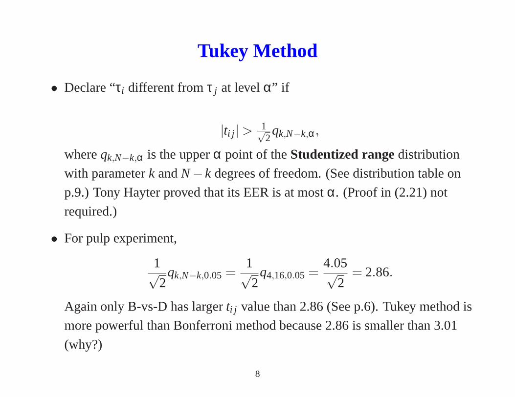
Tukey Method

• Declare “τi different fromτ j at levelα” if

|ti j | > 1√2qk,N−k,α,

whereqk,N−k,α is the upperα point of theStudentized rangedistribution

with parameterk andN−k degrees of freedom. (See distribution table on

p.9.) Tony Hayter proved that its EER is at mostα. (Proof in (2.21) not

required.)

• For pulp experiment,

1√2

qk,N−k,0.05 =1√2

q4,16,0.05 =4.05√

2= 2.86.

Again only B-vs-D has largerti j value than 2.86 (See p.6). Tukey method is

more powerful than Bonferroni method because 2.86 is smallerthan 3.01

(why?)

8

Selected values ofqk,ν,α for α = 0.05

k

ν 2 3 4 5 6 7 8 9 10 11 12 13 14 15

1 17.97 26.98 32.82 37.08 40.41 43.12 45.40 47.36 49.07 50.59 51.96 53.20 54.33 55.36

2 6.08 8.33 9.80 10.88 11.74 12.44 13.03 13.54 13.99 14.39 14.75 15.08 15.38 15.65

3 4.50 5.91 6.82 7.50 8.04 8.48 8.85 9.18 9.46 9.72 9.95 10.15 10.35 10.52

4 3.93 5.04 5.76 6.29 6.71 7.05 7.35 7.60 7.83 8.03 8.21 8.37 8.52 8.66

5 3.64 4.60 5.22 5.67 6.03 6.33 6.58 6.80 6.99 7.17 7.32 7.47 7.60 7.72

6 3.46 4.34 4.90 5.30 5.63 5.90 6.12 6.32 6.49 6.65 6.79 6.92 7.03 7.14

7 3.34 4.16 4.68 5.06 5.36 5.61 5.82 6.00 6.16 6.30 6.43 6.55 6.66 6.76

8 3.26 4.04 4.53 4.89 5.17 5.40 5.60 5.77 5.92 6.05 6.18 6.29 6.39 6.48

9 3.20 3.95 4.41 4.76 5.02 5.24 5.43 5.59 5.74 5.87 5.98 6.09 6.19 6.28

10 3.15 3.88 4.33 4.65 4.91 5.12 5.30 5.46 5.60 5.72 5.83 5.93 6.03 6.11

11 3.11 3.82 4.26 4.57 4.82 5.03 5.20 5.35 5.49 5.61 5.71 5.81 5.90 5.98

12 3.08 3.77 4.20 4.51 4.75 4.95 5.12 5.27 5.39 5.51 5.61 5.71 5.80 5.88

13 3.06 3.73 4.15 4.45 4.69 4.88 5.05 5.19 5.32 5.43 5.53 5.63 5.71 5.79

14 3.03 3.70 4.11 4.41 4.64 4.83 4.99 5.13 5.25 5.36 5.46 5.55 5.64 5.71

15 3.01 3.67 4.08 4.37 4.59 4.78 4.94 5.08 5.20 5.31 5.40 5.49 5.57 5.65

16 3.00 3.65 4.05 4.33 4.56 4.74 4.90 5.03 5.15 5.26 5.35 5.44 5.52 5.59

α=upper tail probability,ν=degrees of freedom,k=number of treatments

For complete tables corresponding to various values ofα refer to Appendix E.

9

One-Way ANOVA with a Quantitative Factor

• Data :

y = bonding strength of composite material,

x = laser power at 40, 50, 60 watt.

Table 2: Strength Data, Composite Experiment

Laser Power (watts)

40 50 60

25.66 29.15 35.73

28.00 35.09 39.56

20.65 29.79 35.66

10

One-Way ANOVA (Contd)

Table 3: ANOVA Table, Composite Experiment

Degrees of Sum of Mean

Source Freedom Squares SquaresF

laser 2 224.184 112.092 11.32

residual 6 59.422 9.904

total 8 283.606

• Conclusion from ANOVA : Laser power has a significant effect on strength.

• To further understand the effect, use of multiple comparisons is not useful

here. ( Why? )

• The effects of a quantitative factor like laser power can be decomposed into

linear, quadratic, etc.

11

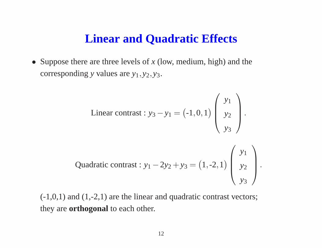
Linear and Quadratic Effects

• Suppose there are three levels ofx (low, medium, high) and the

correspondingy values arey1,y2,y3.

Linear contrast :y3−y1 =(

-1,0,1)

y1

y2

y3

.

Quadratic contrast :y1−2y2 +y3 =(

1, -2,1)

y1

y2

y3

.

(-1,0,1) and (1,-2,1) are the linear and quadratic contrast vectors;

they areorthogonal to each other.

12

Linear and Quadratic Effects (Contd.)

• Using (-1,0,1) and (1,-2,1), we can write a more detailed regression model

y = Xβ+ ε, where the model matrixX is given as in (2.26).

• Normalization : Length of(−1,0,1) =√

2, length of(1,−2,1) =√

6,

divide each vector by its length in the regression model. (Why ? It provides

aconsistentcomparison of the regression coefficients. But thet-statistics in

the next table are independent of such (and any) scaling.)

• Normalized contrast vectors:

linear: (−1,0,1)/√

2 = (−1/√

2,0,1/√

2),

quadratic:(1,−2,1)/√

6 = (1/√

6,−2/√

6,1/√

6).

13

Estimation of Linear and Quadratic Effects• Let β0, βl , βq denote respectively the intercept, the linear effect and the quadratic

effect and letβ = (β0,βl ,βq)′. An estimatorβ of β based on normalized constrasts

for the mean, linear, and quadratic effects is given by

β =

β0

βl

βq

=

1/√

3 1/√

3 1/√

3

−1/√

2 0 1/√

2

1/√

6 −2/√

6 1/√

6

y1

y2

y3

• We can writeβ = X′y, where

X =

1/√

3 −1/√

2 1/√

6

1/√

3 0 −2/√

6

1/√

3 1/√

2 1/√

6

• Since the columns ofX constitute a set of orthonormal vectors, i.e.X′X = I , we have

β = X′y = (X′X)−1X′y.

This shows thatβ is identical to the least squares estimate ofβ.

• Running a multiple linear regression with responsey and predictorsxl andxq, we get

β0 = 31.0322, βl = 8.636, βq = −0.381.

14

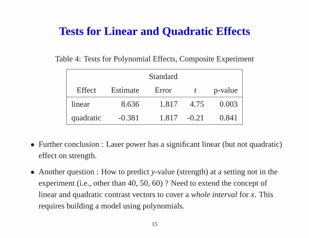
Tests for Linear and Quadratic Effects

Table 4: Tests for Polynomial Effects, Composite Experiment

Standard

Effect Estimate Error t p-value

linear 8.636 1.817 4.75 0.003

quadratic -0.381 1.817 -0.21 0.841

• Further conclusion : Laser power has a significant linear (but not quadratic)

effect on strength.

• Another question : How to predicty-value (strength) at a setting not in the

experiment (i.e., other than 40, 50, 60) ? Need to extend the concept of

linear and quadratic contrast vectors to cover awhole intervalfor x. This

requires building a model using polynomials.

15

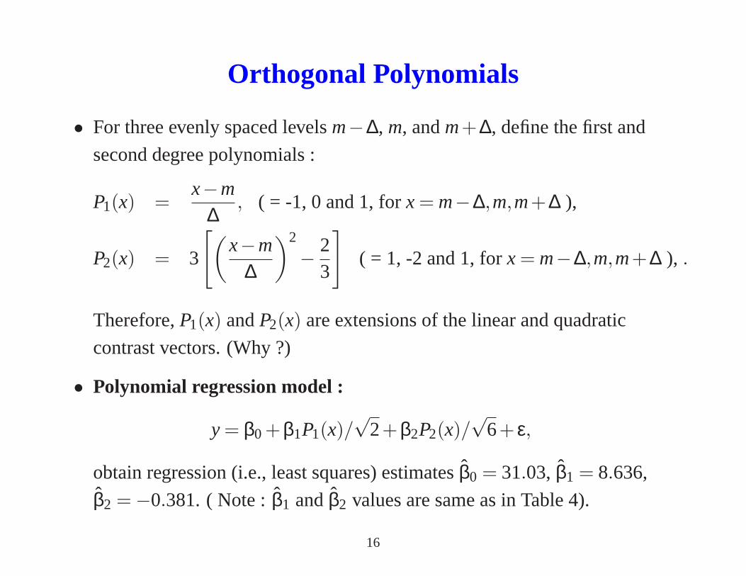
Orthogonal Polynomials

• For three evenly spaced levelsm−∆, m, andm+∆, define the first and

second degree polynomials :

P1(x) =x−m

∆, ( = -1, 0 and 1, forx = m−∆,m,m+∆ ),

P2(x) = 3

[

(

x−m∆

)2

− 23

]

( = 1, -2 and 1, forx = m−∆,m,m+∆ ), .

Therefore,P1(x) andP2(x) are extensions of the linear and quadratic

contrast vectors. (Why ?)

• Polynomial regression model :

y = β0 +β1P1(x)/√

2+β2P2(x)/√

6+ ε,

obtain regression (i.e., least squares) estimatesβ0 = 31.03, β1 = 8.636,

β2 = −0.381. ( Note :β1 andβ2 values are same as in Table 4).

16

Prediction based on Polynomial Regression Model

• Fitted model:

y = 31.0322+8.636P1(x)/√

2−0.381P2(x)/√

6,

• To predicty at anyx, plug in thex on the right side of the regression

equation. Forx = 55= 50+ 1210,m= 50,∆ = 10,

P1(55) =55−50

10=

12,

P2(55) = 3

[

(

55−5010

)2

− 23

]

= −54,

y = 31.0322+8.636(0.3536)−0.381(−0.5103)

= 34.2803.

17

Residual Analysis: Theory

• Theory: define theresidual for the ith observationxi as

r i = yi − yi , yi = xTi β,

yi contains information given by the model;r i is the “difference” betweenyi

(observed) and ˆyi(fitted) and contains information on possiblemodel

inadequacy.

Vector of residualsr = {r i}Ni=1 = y−Xβ.

• Under the model assumptionE(y) = Xβ, it can be shown that

(a)E(r) = 0,

(b) r andy are independent,

(c) variances ofr i are nearly constant for “nearly balanced” designs.

18

Residual Plots

• Plot r i vs. yi (see Figure 1): It should appear as a parallel band around 0.

Otherwise, it would suggest model violation. If spread ofr i increases as ˆyi

increases, error variance ofy increases with mean ofy. Need a

transformation ofy. (Will be explained in Unit 3.)

• Plot r i vs. xi (see Figure 2): If not a parallel band around 0, relationship

betweenyi andxi not fully captured, revise theXβ part of the model.

• Plot r i vs. time sequence: to see if there is a time trend or autocorrelation

over time.

• Plot r i from replicates per treatment: to see if error variance depends on

treatment.

19

Plot of r i vs. yi

•

•

•

•

•

•

•

•

•

•

•

•

•

•

•

•

•

fitted

resid

ua

l

60.1 60.2 60.3 60.4 60.5 60.6 60.7

-0.4

-0.2

0.0

0.2

0.4

0.6

Figure 1:r i vs. yi , Pulp Experiment

20

Plot of r i vs.xi

•

•

•

•

•

•

•

•

•

•

•

•

•

•

•

•

•

operator

resid

ua

l

-0.4

-0.2

0.0

0.2

0.4

0.6

A B C D

Figure 2:r i vs.xi , Pulp Experiment

21

Box-Whisker Plot

• A powerful graphical display (due to Tukey) to capture the location,

dispersion, skewness and extremity of a distribution. See Figure 3.

• Q1 = lower quartile (25th percentile),Q3 = upper quartile (75th percentile),

Q2 = median (location) is the white line in the box.Q1 andQ3 are

boundaries of theblack box.

IQR= interquartile range (length of box) =Q3 - Q1 is a measure of

dispersion.

Minimum and maximum ofobservedvalues within

[Q1−1.5IQR,Q3 +1.5IQR] are denoted by twowhiskers. Any values

outside the whiskers areoutliersand are displayed.

• If Q1 andQ3 are not symmetric around the median, it indicatesskewness.

22

Box-Whisker Plot

Figure 3: Box-Whisker Plot

23

Normal Probability Plot

• Original purpose : To test if a distribution is normal, e.g., ifthe residuals

follow a normal distribution (see Figure 5). More powerful use in factorial

experiments (will be discussed in Units 4 and 5).

• Let r(1) ≤ . . . ≤ r(N) be the ordered residuals. The cumulative probability for

r(i) is pi = (i −0.5)/N. Thus the plot ofpi vs. r(i) should be S-shaped as in

Figure 4(a) if the errors are normal. By transforming the scale of the

horizontal axis, the S-shaped curve is straightened to be a line (see

Figure 4(b)).

• Normal probability plot of residuals :(

Φ−1(pi), r(i))

, i = 1, . . . ,N, Φ = normal cdf.

If the errors are normal, it should plot roughly as a straightline. See

Figure 5.

24

Regular and Normal Probability Plots of Normal

CDF(a)

-2 -1 0 1 2

0.2

0.4

0.6

0.8

1.0

(b)

-2 -1 -0.5 0 0.5 1 2

0.2

0.4

0.6

0.8

1.0

Figure 4: Normal Plot ofr i , Pulp Experiment

25

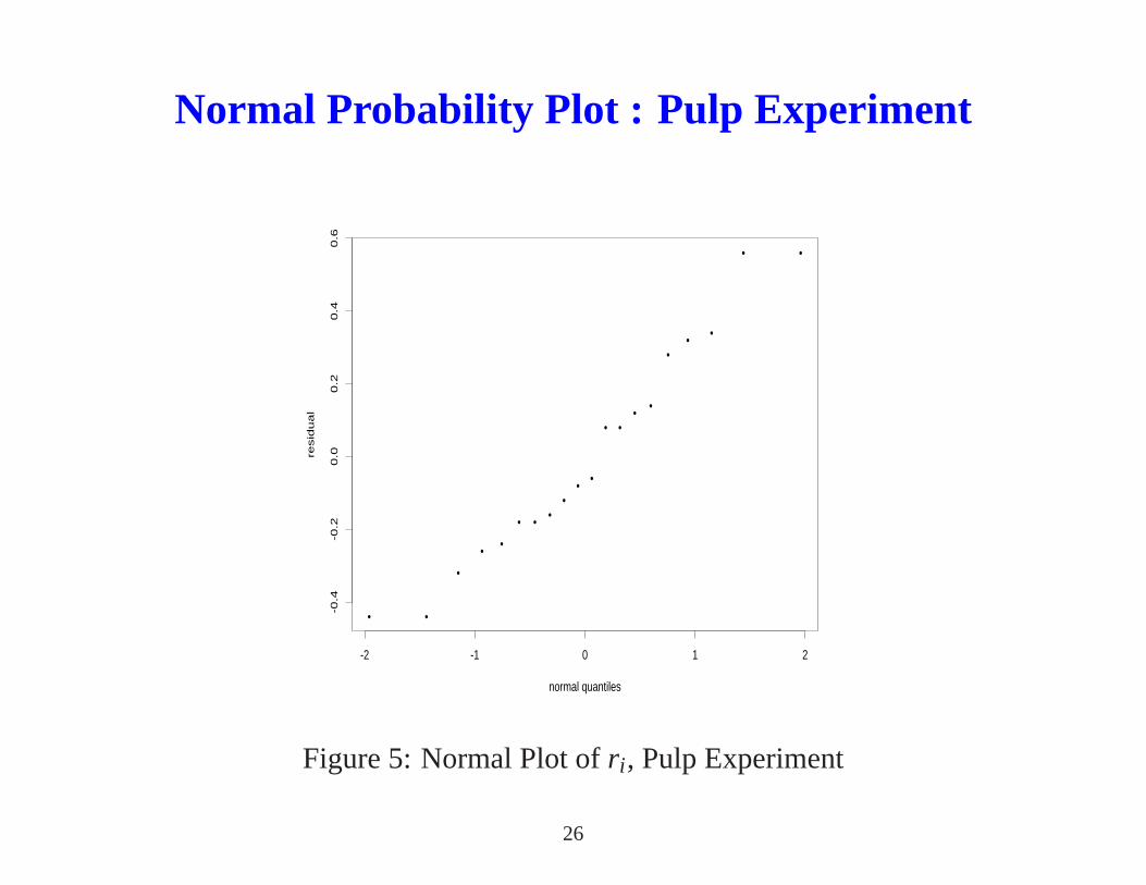
Normal Probability Plot : Pulp Experiment

•

•

• •

•

•

•

•

•

•

• •

•

•

•

•

•

•

• •

normal quantiles

resid

ua

l

-2 -1 0 1 2

-0.4

-0.2

0.0

0.2

0.4

0.6

Figure 5: Normal Plot ofr i , Pulp Experiment

26

Pulp Experiment Revisited

• In the pulp experiment the effectsτi are calledfixedeffects because the

interest was in comparing the fourspecificoperators in the study. If these

four operators were chosen randomly from the population of operators in

the plant, the interest would usually be in the variation among all operators

in the population. Because the observed data are from operators randomly

selected from the population, the variation among operators in the

populationis referred to asrandomeffects.

• One-way random effects model :

yi j = η+ τi + εi j ,

εi j ’s are independent error terms withN(0,σ2), τi are independentN(0,σ2τ),

andτi andεi j are independent (Why? Give an example.);σ2 andσ2τ are the

two variance componentsof the model. The variance among operators in

the population is measured byσ2τ .

27

One-way Random Effects Model: ANOVA and

Variance Components

• The null hypothesis for the fixed effects model:τ1 = · · · = τk should be

replaced by

H0 : σ2τ = 0.

UnderH0, theF test and the ANOVA table in Section 2.1 still holds.

Reason: underH0, SSTr∼ σ2χ2k−1 andSSE∼ σ2χ2

N−k. Therefore theF-test

has the distributionFk−1,N−k underH0.

• We can apply thesameANOVA andF test in the fixed effects case for

analyzing data. For example, using the results in Section 2.1, theF test has

value 4.2 and thusH0 is rejected at level 0.05. However, we need to

compute the expected mean squares under the alternative ofσ2τ > 0,

(i) for sample size determination, and

(ii) to estimate the variance components.

28

Expected Mean Squares for Treatments

• Equation (1) holds independent ofσ2τ ,

E(MSE) = E

(

SSEN−k

)

= σ2. (1)

• Under the alternative:σ2τ > 0, and forni = n,

E(MSTr) = E

(

SSTrk−1

)

= σ2 +nσ2τ . (2)

For unequalni ’s, n in (2) is replaced by

n′ =1

k−1

[

k

∑i=1

ni −∑k

i=1n2i

∑ki=1ni

]

.

29

Proof of (2)

yi. − y.. =(

τi − τ.

)

+(

εi .− ε..

)

SSTr =k

∑i=1

n(

yi. − y..

)2

= n{

∑(

τi − τ.

)2+∑

(

εi. − ε..

)2+2∑

(

εi. − ε..

)(

τi − τ.

)

}

.

The cross product term has mean 0 (becauseτ andε are independent). It can beshown that

E( k

∑i=1

(

τi − τ.

)2)

= (k−1)σ2τ and E

( k

∑i=1

(

εi. − ε..

)2)

=(k−1)σ2

n.

Therefore

E(SSTr) = n(k−1)σ2τ +(k−1)σ2,

E(MSTr) = E

(

SSTrk−1

)

= σ2 +nσ2τ .

30

ANOVA Tables (ni = n)

Source d.f. SS MS E(MS)

treatment k−1 SSTr MSTr= SSTrk−1 σ2 +nσ2

τ

residual N−k SSE MSE= SSEN−k σ2

total N−1

Pulp Experiment

Source d.f. SS MS E(MS)

treatment 3 1.34 0.447 σ2 +5σ2τ

residual 16 1.70 0.106 σ2

total 19 3.04

31

Estimation of σ2 and σ2τ

• From equations (1) and (2), we obtain the following unbiasedestimates ofthe variance components:

σ2 = MSE and σ2τ =

MSTr−MSEn

.

Note thatσ2τ ≥ 0 if and only ifMSTr≥ MSE, which is equivalent toF ≥ 1.

Therefore anegativevariance estimateσ2τ occurs only if the value of theF

statistic is less than 1. Obviously the null hypothesisH0 is not rejected whenF ≤ 1. Since variance cannot be negative, a negative variance estimate isreplaced by 0. This does not mean thatσ2

τ is zero. It simply means that thereis not enough information in the data to get a good estimate ofσ2

τ .

• For the pulp experiment,n = 5, σ2 = 0.106,σ2τ = (0.447−0.106)/5 = 0.068,

i.e., sheet-to-sheet variance (within same operator) is 0.106, which is about50% higher than operator-to-operator variance 0.068.

Implications on process improvement(discuss in class) : try to reduce thetwo sources of variation, also considering costs.

32

Estimation of Overall Mean η• In random effects model,η, the population mean, is often of interest.

FromE(yi j ) = η, we use the estimate

η = y.. .

• Var(η) = Var(τ. + ε..) =σ2

τk + σ2

N , whereN = ∑ki=1ni .

Forni = n, Var(η) =σ2

τk + σ2

nk = 1nk

(

σ2 +nσ2τ)

.

Using (2),MSTrnk is an unbiased estimate ofVar(η). Confidence interval for

η:

η± tk−1, α2

√

MSTrnk

• In the pulp experiment,η = 60.40,MSTr= 0.447, and the 95% confidenceinterval forη is

60.40±3.182

√

0.4475×4

= [59.92,60.88].

33

Comments on Board

34