uncertainty propagation for terrestrial mobile laser …

UNCERTAINTY PROPAGATION FOR TERRESTRIAL MOBILE LASER SCANNER

Miloud Mezian* , Bruno Vallet *, Bahman Soheilian*, Nicolas Paparoditis*

* Universite Paris-Est, IGN, SRIG, MATIS, 73 avenue de Paris, 94160 Saint Mande, France

([email protected])

Commission III, WG III/2

KEY WORDS: Mobile mapping, Laser scanner, Uncertainty propagation, Error ellipsoid

ABSTRACT:

Laser scanners are used more and more in mobile mapping systems. They provide 3D point clouds that are used for object reconstructionand registration of the system. For both of those applications, uncertainty analysis of 3D points is of great interest but rarely investigatedin the literature. In this paper we present a complete pipeline that takes into account all the sources of uncertainties and allows tocompute a covariance matrix per 3D point. The sources of uncertainties are laser scanner, calibration of the scanner in relation tothe vehicle and direct georeferencing system. We suppose that all the uncertainties follow the Gaussian law. The variances of thelaser scanner measurements (two angles and one distance) are usually evaluated by the constructors. This is also the case for integrateddirect georeferencing devices. Residuals of the calibration process were used to estimate the covariance matrix of the 6D transformationbetween scanner laser and the vehicle system. Knowing the variances of all sources of uncertainties, we applied uncertainty propagationtechnique to compute the variance-covariance matrix of every obtained 3D point. Such an uncertainty analysis enables to estimate theimpact of different laser scanners and georeferencing devices on the quality of obtained 3D points. The obtained uncertainty valueswere illustrated using error ellipsoids on different datasets.

1. INTRODUCTION

Mobile Terrestrial LiDAR System (MTLS) is an emerging tech-nology that combines the use of a laser scanner, Global Naviga-tion System (GPS), Inertial Navigation System (INS) and odome-ter on a mobile platform to produce accurate and precise geospa-tial data on canyon urban. Much more detailed information hasbeen acquired in comparaison with Airborne LiDAR Systems(ALS). (Olsen, 2013) discussed the key differences and similar-ties between airborne and mobile LiDAR data. The MTLS allowsto obtain a large amount of 3D positional information in a fast andefficient way, which can be used in numerous applications, suchas the object reconstruction and registration of system. In suchapplications, uncertainty analysis of 3D points is of great interestbut rarely investigated in the literature. Consequently, it is impor-tant for users to know the uncertainty of MTLS and the factorsthat can influence the quality of 3D scanned data. Several studieshave analysed the sources of uncertainties in MTLS, which aresimilar to those used by Airborne LiDAR System (ALS). Moredetail about ALS uncertainty sources was introduced by (Schaeret al., 2007). Others issues, related to sources of uncertainty af-fecting on the accuracy of the Mobile Terrestrial LiDAR pointcloud are discussed in (Alshawa et al., 2007, Olsen, 2013, Leslaret al., 2014, Poreba, 2014) .

In general, the sources of uncertainty are divided into three maincategories:

• navigation uncertainties : Here we have uncertainty of theabsolute position and the vehicule orientation measured byINS in real time. The factors that affect the accuracy of thevehicule’s position depend : multipath, shading of the sig-nals caused by buildings and trees, and poor GPS satellitegeometry (Glennie, 2007, Haala et al., 2008). Under goodGPS conditions this uncertainty is about few centimeters,

however, under difficult conditions it can be up to few me-ters. In (Leslar et al., 2014), they have proved that undertightly controlled error conditions, the source of uncertaintyin point cloud is domined by vehicule position.

• calibration uncertainties : Namely the uncertainties in theleverarm and in the boresight angles between scanner laserand the INS frame. The quality of the calibration parametersis usually known and depends on the calibration procedure(Le Scouarnec et al., 2014, Rieger et al., 2010).

• laser scanning uncertainties : The scanner laser measure-ments consist of two angulars and one distance.The factorsaffecting laser-target position accuracy are numerous suchas the weather (humidity, temperature), properties of thescanned surface (roughness, reflectivity), scanning geom-etry (incidence angle on the surface) and scanner mecha-nism precision (mirror center offset) (Soudarissanane et al.,2008). These uncertainties are evaluated by the construc-tors.

This paper is organized as follows: Section 1 presents briefly theprinciples of geo-referencing of 3D point. Section 2 describes acomplete pipeline that takes into account all the sources of uncer-tainties and allows to compute a covariance matrix per 3D point.The obtained uncertainty values were illustrated using error ellip-soids on different datasets.

In this work, the mobile data that we used was produced by theterrestrial mobile mapping vehicle Stereopolis II (Paparoditis etal., 2012) developped at National Geographic Institute (IGN).The laser sensor is a RIEGL VQ-250 that was mounted transver-sally in order to scan a plane orthogonal to the trajectory. It ro-tates at 100 Hz and emits 3000 pulses per rotation, which cor-responds to an angular resolution around 0.12 result in 0 to 8echoes producing an average of 250 thousand points per second.

The International Archives of the Photogrammetry, Remote Sensing and Spatial Information Sciences, Volume XLI-B3, 2016 XXIII ISPRS Congress, 12–19 July 2016, Prague, Czech Republic

This contribution has been peer-reviewed. doi:10.5194/isprsarchives-XLI-B3-331-2016

331

1.1 Mobile Terrestrial LiDAR formulas

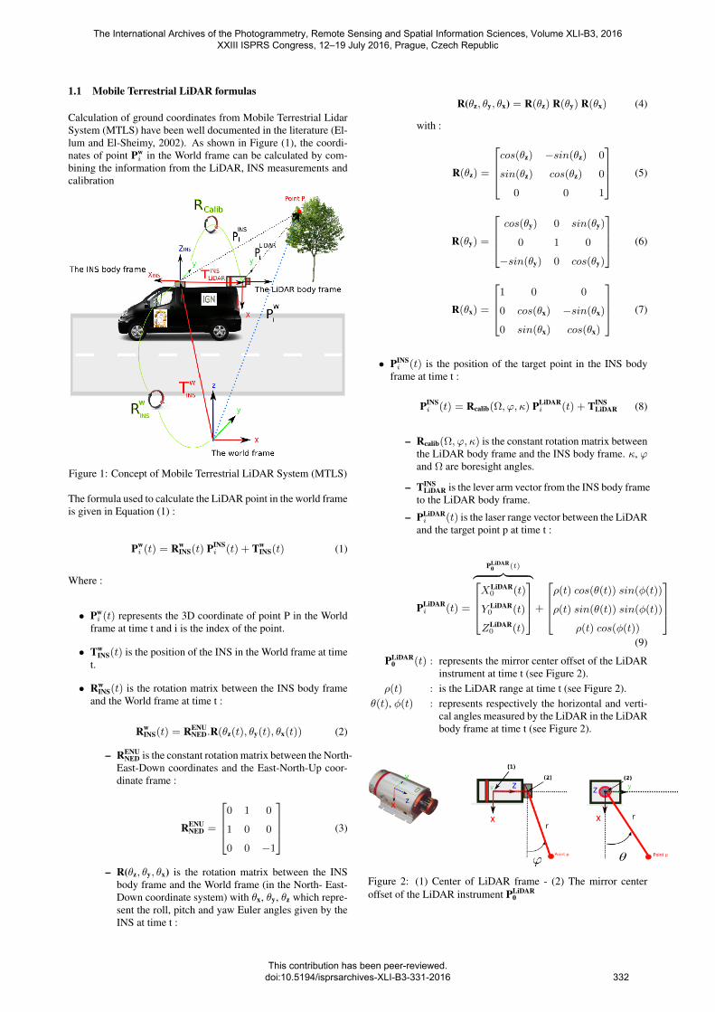
Calculation of ground coordinates from Mobile Terrestrial LidarSystem (MTLS) have been well documented in the literature (El-lum and El-Sheimy, 2002). As shown in Figure (1), the coordi-nates of point Pw

i in the World frame can be calculated by com-bining the information from the LiDAR, INS measurements andcalibration

Figure 1: Concept of Mobile Terrestrial LiDAR System (MTLS)

The formula used to calculate the LiDAR point in the world frameis given in Equation (1) :

Pwi (t) = Rw

INS(t) PINSi (t) + Tw

INS(t) (1)

Where :

• Pwi (t) represents the 3D coordinate of point P in the World

frame at time t and i is the index of the point.

• TwINS(t) is the position of the INS in the World frame at time

t.

• RwINS(t) is the rotation matrix between the INS body frame

and the World frame at time t :

RwINS(t) = RENU

NED.R(θz(t), θy(t), θx(t)) (2)

– RENUNED is the constant rotation matrix between the North-

East-Down coordinates and the East-North-Up coor-dinate frame :

RENUNED =

0 1 0

1 0 0

0 0 −1

(3)

– R(θz, θy, θx) is the rotation matrix between the INSbody frame and the World frame (in the North- East-Down coordinate system) with θx, θy, θz which repre-sent the roll, pitch and yaw Euler angles given by theINS at time t :

R(θz, θy, θx) = R(θz) R(θy) R(θx) (4)

with :

R(θz) =

cos(θz) −sin(θz) 0

sin(θz) cos(θz) 0

0 0 1

(5)

R(θy) =

cos(θy) 0 sin(θy)

0 1 0

−sin(θy) 0 cos(θy)

(6)

R(θx) =

1 0 0

0 cos(θx) −sin(θx)

0 sin(θx) cos(θx)

(7)

• PINSi (t) is the position of the target point in the INS body

frame at time t :

PINSi (t) = Rcalib(Ω, ϕ, κ) PLiDAR

i (t) + TINSLiDAR (8)

– Rcalib(Ω, ϕ, κ) is the constant rotation matrix betweenthe LiDAR body frame and the INS body frame. κ, ϕand Ω are boresight angles.

– TINSLiDAR is the lever arm vector from the INS body frame

to the LiDAR body frame.

– PLiDARi (t) is the laser range vector between the LiDAR

and the target point p at time t :

PLiDARi (t) =

PLiDAR0 (t)︷︸︸︷

XLiDAR0 (t)

Y LiDAR0 (t)

ZLiDAR0 (t)

+

ρ(t) cos(θ(t)) sin(φ(t))

ρ(t) sin(θ(t)) sin(φ(t))

ρ(t) cos(φ(t))

(9)

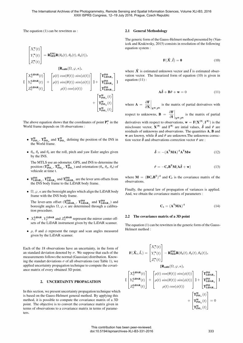
PLiDAR0 (t) : represents the mirror center offset of the LiDAR

instrument at time t (see Figure 2).ρ(t) : is the LiDAR range at time t (see Figure 2).

θ(t), φ(t) : represents respectively the horizontal and verti-cal angles measured by the LiDAR in the LiDARbody frame at time t (see Figure 2).

Figure 2: (1) Center of LiDAR frame - (2) The mirror centeroffset of the LiDAR instrument PLiDAR

0



332

The equation (1) can be rewritten as :

Xwi (t)

Y wi (t)

Zwi (t)

= RENUNEDR(θz(t), θy(t), θx(t)).

[Rcalib(Ω, ϕ, κ).

[

XLiDAR

0 (t)

Y LiDAR0 (t)

ZLiDAR0 (t)

+



ρ(t) cos(φ(t))

] +

TINS

LiDARx

TINSLiDARy

TINSLiDARz

]

+

TW

INSx(t)

TWINSy (t)

TWINSz (t)

The above equation shows that the coordinates of point Pwi in the

World frame depends on 18 observations :

• TWINSx , TW

INSy and TWINSz defining the position of the INS in

the World frame.

• θx, θy and θz are the roll, pitch and yaw Euler angles givenby the INS.

The MTLS use an odometer, GPS, and INS to determine theposition (TW

INSx , TWINSy , TW

INSz ) and orientation (θx, θy, θz) ofvehicule at time t.

• TINSLiDARx

, TINSLiDARy

and TINSLiDARz

are the lever arm offsets fromthe INS body frame to the LiDAR body frame.

• Ω, ϕ, κ are the boresight angles which align the LiDAR bodyframe with the INS body frame.

The lever-arm offset (TINSLiDARx

, TINSLiDARy

and TINSLiDARz

) andboresight angles Ω, ϕ, κ are determined through a calibra-tion procedure.

• XLiDAR0 , Y LiDAR

0 and ZLiDAR0 represent the mirror center off-

sets of the LiDAR instrument given by the LiDAR scanner.

• ρ, θ and φ represent the range and scan angles measuredgiven by the LiDAR scanner.

Each of the 18 observations have an uncertainty, in the form ofan standard deviation denoted by σ. We suppose that each of themeasurements follows the normal (Gaussian) distribution. Know-ing the standart deviations σ of all observations (see Table 1), weapplied uncertainty propagation technique to compute the covari-ance matrix of every obtained 3D point.

2. UNCERTAINTY PROPAGATION

In this section, we present uncertainty propagation technique whichis based on the Gauss-Helmert general method. By applying thismethod, it is possible to compute the covariance matrix of a 3Dpoint. The objective is to convert the covariance matrix given interms of observations to a covariance matrix in terms of parame-ters.

2.1 General Methodology

The generic form of the Gauss-Helmert method presented by (Van-icek and Krakiwsky, 2015) consists in resolution of the followingequation system :

F(X, l) = 0 (10)

where X is estimated unknown vector and l is estimated obser-vation vector. The linearized form of equation (10) is given inequation (11) :

Aδ + Br + w = 0 (11)

where A =∂F∂X

∣∣∣∣X(0),l(0)

is the matrix of partial derivatives with

respect to unknowns, B =∂F∂l

∣∣∣∣X(0),l(0)

is the matrix of partial

derivatives with respect to observations, w = F(X(0), l(0)) is themisclosure vector, X(0) and l(0) are intial values, δ and r areresiduals of unknowns and observations. The quantities A, B andw are known, while δ and r are unknown.The unknowns correc-tion vector δ and observations correction vector r are :

δ = −(ATMA)-1ATMw (12)

r = −CrBTM(Aδ + w) (13)

where M = (BCrBT)-1 and Cr is the covariance matrix of theobservations.

Finally, the general law of propagation of variances is applied.And, we obtain the covariance matrix of parameters :

Cx = (ATMA)-1 (14)

2.2 The covariance matrix of a 3D point

The equation (1) can be rewritten in the generic form of the Gauss-Helmert method :

F(Xi, li) =

Xwi (t)

Y wi (t)

Zwi (t)

− RENUNEDR(θz(t), θy(t), θx(t)).

[Rcalib(Ω, ϕ, κ).

[

XLiDAR

0 (t)

Y LiDAR0 (t)

ZLiDAR0 (t)

+



ρ(t) cos(φ(t))

] +

TINS

LiDARx

TINSLiDARy

TINSLiDARz

]

+

TW

INSx(t)

TWINSy (t)

TWINSz (t)

= 0



333

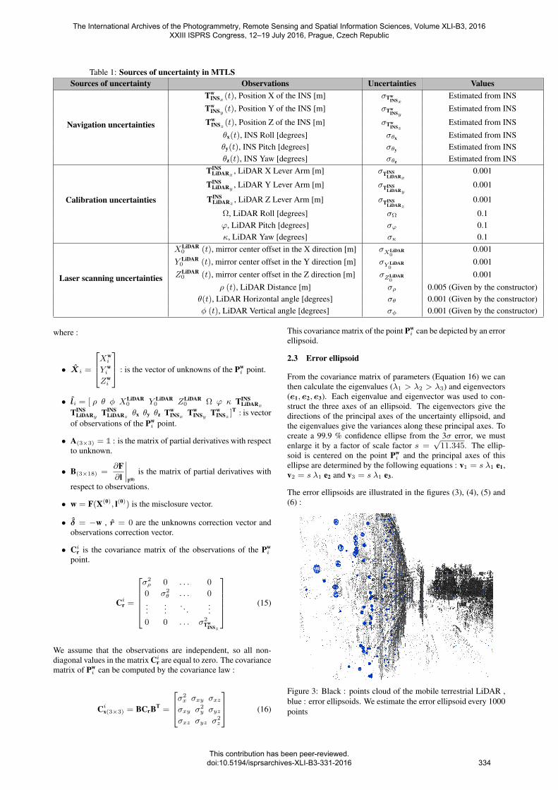
Table 1: Sources of uncertainty in MTLSSources of uncertainty Observations Uncertainties Values

Navigation uncertainties

TwINSx(t), Position X of the INS [m] σTw

INSxEstimated from INS

TwINSy (t), Position Y of the INS [m] σTw

INSyEstimated from INS

TwINSz (t), Position Z of the INS [m] σTw

INSzEstimated from INS

θx(t), INS Roll [degrees] σθx Estimated from INSθy(t), INS Pitch [degrees] σθy Estimated from INSθz(t), INS Yaw [degrees] σθz Estimated from INS

Calibration uncertainties

TINSLiDARx

, LiDAR X Lever Arm [m] σTINSLiDARx

0.001

TINSLiDARy

, LiDAR Y Lever Arm [m] σTINSLiDARy

0.001

TINSLiDARz

, LiDAR Z Lever Arm [m] σTINSLiDARz

0.001

Ω, LiDAR Roll [degrees] σΩ 0.1ϕ, LiDAR Pitch [degrees] σϕ 0.1κ, LiDAR Yaw [degrees] σκ 0.1

Laser scanning uncertainties

XLiDAR0 (t), mirror center offset in the X direction [m] σXLiDAR

00.001

Y LiDAR0 (t), mirror center offset in the Y direction [m] σY LiDAR

00.001

ZLiDAR0 (t), mirror center offset in the Z direction [m] σZLiDAR

00.001

ρ (t), LiDAR Distance [m] σρ 0.005 (Given by the constructor)θ(t), LiDAR Horizontal angle [degrees] σθ 0.001 (Given by the constructor)φ (t), LiDAR Vertical angle [degrees] σφ 0.001 (Given by the constructor)

where :

• Xi =

Xwi

Y wi

Zwi

: is the vector of unknowns of the Pwi point.

• li = [ ρ θ φ XLiDAR0 Y LiDAR

0 ZLiDAR0 Ω ϕ κ TINS

LiDARx

TINSLiDARy

TINSLiDARz

θx θy θz TwINSx Tw

INSy TwINSz ]T : is vector

of observations of the Pwi point.

• A(3×3) = 1 : is the matrix of partial derivatives with respectto unknown.

• B(3×18) =∂F∂l

∣∣∣∣l(0)

is the matrix of partial derivatives with

respect to observations.

• w = F(X(0), l(0)) is the misclosure vector.

• δ = −w , r = 0 are the unknowns correction vector andobservations correction vector.

• Cir is the covariance matrix of the observations of the Pwi

point.

Cir =

σ2ρ 0 . . . 0

0 σ2θ . . . 0

......

. . ....

0 0 . . . σ2Tw

INSz

(15)

We assume that the observations are independent, so all non-diagonal values in the matrix Cir are equal to zero. The covariancematrix of Pw

i can be computed by the covariance law :

Cix(3×3) = BCrBT =

σ2x σxy σxzσxy σ2

y σyzσxz σyz σ2

z

(16)

This covariance matrix of the point Pwi can be depicted by an error

ellipsoid.

2.3 Error ellipsoid

From the covariance matrix of parameters (Equation 16) we canthen calculate the eigenvalues (λ1 > λ2 > λ3) and eigenvectors(e1, e2, e3). Each eigenvalue and eigenvector was used to con-struct the three axes of an ellipsoid. The eigenvectors give thedirections of the principal axes of the uncertainty ellipsoid, andthe eigenvalues give the variances along these principal axes. Tocreate a 99.9 % confidence ellipse from the 3σ error, we mustenlarge it by a factor of scale factor s =

√11.345. The ellip-

soid is centered on the point Pwi and the principal axes of this

ellipse are determined by the following equations : v1 = s λ1 e1,v2 = s λ1 e2 and v3 = s λ1 e3.

The error ellipsoids are illustrated in the figures (3), (4), (5) and(6) :

Figure 3: Black : points cloud of the mobile terrestrial LiDAR ,blue : error ellipsoids. We estimate the error ellipsoid every 1000points



334

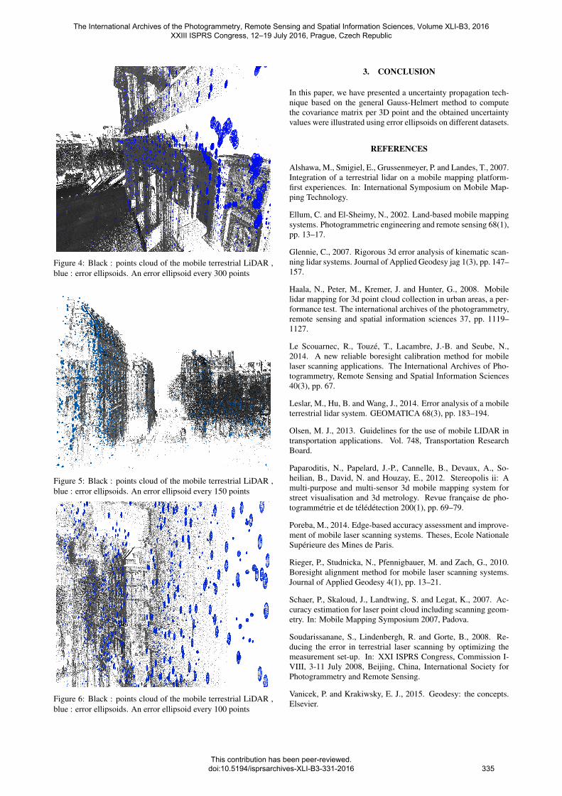
Figure 4: Black : points cloud of the mobile terrestrial LiDAR ,blue : error ellipsoids. An error ellipsoid every 300 points



3. CONCLUSION

In this paper, we have presented a uncertainty propagation tech-nique based on the general Gauss-Helmert method to computethe covariance matrix per 3D point and the obtained uncertaintyvalues were illustrated using error ellipsoids on different datasets.

REFERENCES

Alshawa, M., Smigiel, E., Grussenmeyer, P. and Landes, T., 2007.Integration of a terrestrial lidar on a mobile mapping platform-first experiences. In: International Symposium on Mobile Map-ping Technology.

Ellum, C. and El-Sheimy, N., 2002. Land-based mobile mappingsystems. Photogrammetric engineering and remote sensing 68(1),pp. 13–17.

Glennie, C., 2007. Rigorous 3d error analysis of kinematic scan-ning lidar systems. Journal of Applied Geodesy jag 1(3), pp. 147–157.

Haala, N., Peter, M., Kremer, J. and Hunter, G., 2008. Mobilelidar mapping for 3d point cloud collection in urban areas, a per-formance test. The international archives of the photogrammetry,remote sensing and spatial information sciences 37, pp. 1119–1127.

Le Scouarnec, R., Touze, T., Lacambre, J.-B. and Seube, N.,2014. A new reliable boresight calibration method for mobilelaser scanning applications. The International Archives of Pho-togrammetry, Remote Sensing and Spatial Information Sciences40(3), pp. 67.

Leslar, M., Hu, B. and Wang, J., 2014. Error analysis of a mobileterrestrial lidar system. GEOMATICA 68(3), pp. 183–194.

Olsen, M. J., 2013. Guidelines for the use of mobile LIDAR intransportation applications. Vol. 748, Transportation ResearchBoard.

Paparoditis, N., Papelard, J.-P., Cannelle, B., Devaux, A., So-heilian, B., David, N. and Houzay, E., 2012. Stereopolis ii: Amulti-purpose and multi-sensor 3d mobile mapping system forstreet visualisation and 3d metrology. Revue francaise de pho-togrammetrie et de teledetection 200(1), pp. 69–79.

Poreba, M., 2014. Edge-based accuracy assessment and improve-ment of mobile laser scanning systems. Theses, Ecole NationaleSuperieure des Mines de Paris.

Rieger, P., Studnicka, N., Pfennigbauer, M. and Zach, G., 2010.Boresight alignment method for mobile laser scanning systems.Journal of Applied Geodesy 4(1), pp. 13–21.

Schaer, P., Skaloud, J., Landtwing, S. and Legat, K., 2007. Ac-curacy estimation for laser point cloud including scanning geom-etry. In: Mobile Mapping Symposium 2007, Padova.

Soudarissanane, S., Lindenbergh, R. and Gorte, B., 2008. Re-ducing the error in terrestrial laser scanning by optimizing themeasurement set-up. In: XXI ISPRS Congress, Commission I-VIII, 3-11 July 2008, Beijing, China, International Society forPhotogrammetry and Remote Sensing.

Vanicek, P. and Krakiwsky, E. J., 2015. Geodesy: the concepts.Elsevier.



335

uncertainty propagation for terrestrial mobile laser …

Documents