uncertainty propagation in cfd using polynomial...
TRANSCRIPT
Uncertainty Propagation in CFD Using
Polynomial Chaos Decomposition
O.M. Knio a,∗, O.P. Le Maıtre b
aDepartment of Mechanical Engineering, The Johns Hopkins University,
Baltimore, MD 21218, USA
bUniversite d’Evry Val d’Essonne, CEMIF and Laboratoire d’Informatique pour la
Mecanique et les Sciences de l’Ingenieur,
LIMSI-CNRS, BP 133, F-91403 Orsay, France
Abstract
Uncertainty quantification (UQ) in CFD computations is receiving increased in-terest, due in large part to the increasing complexity of physical models, and theinherent introduction of random model data. This paper focuses on recent applica-tion of Polynomial Chaos (PC) methods for uncertainty representation and propa-gation in CFD computations. The fundamental concept on which Polynomial Chaos(PC) representations are based is to regard uncertainty as generating a new set ofdimensions, and the solution as being dependent on these dimensions. A spectraldecomposition in terms of orthogonal basis functions is used, the evolution of thebasis coefficients providing quantitative estimates of the effect of random modeldata. A general overview of PC applications in CFD is provided, focusing exclu-sively on applications involving the unreduced Navier-Stokes equations. Includedin the present review are an exposition of the mechanics of PC decompositions,an illustration of various means of implementing these representation, a perspec-tive on the applicability of the corresponding techniques to propagate and quantifyuncertainty in Navier-Stokes computations.
Key words: Polynomial Chaos, uncertainty quantification, adaptive scheme
∗ Corresponding author. Tel: 1-410-516-7736; Fax: 1-410-516-7254.Email addresses: [email protected] (O.M. Knio), [email protected]
(O.P. Le Maıtre).
Preprint submitted to Elsevier Science 5 October 2005
1 Introduction
The increasing complexity of physical models in CFD computations is fre-quently accompanied by the introduction of uncertain model data, such asinexact knowledge of system forcing, initial and boundary conditions, physi-cal properties of the medium, as well as parameters in rate expressions. Thesesituations underscore the need for efficient UQ methods, namely for the es-tablishment of confidence intervals in computed predictions, the assessment ofthe suitability of model formulations, and/or the support of decision-makinganalysis. This paper provides a survey of recent applications of PC represen-tations [4, 47] to propagate and quantify uncertainty in CFD computations.
PC methods rely on a probabilistic framework, which distinguishes them fromalternative approaches in uncertainty assessment including fuzzy set theories,interval analysis, convex analysis, as well as linearization and perturbationmethods. The fundamental concept on which PC decompositions are basedis to regard uncertainty as generating a new dimension and the solution asbeing dependent on this dimension. A convergent expansion along the newdimension is then sought in terms of a set of orthogonal basis functions, whosecoefficients can be used to quantify and characterize the uncertainty. Themotivation behind PC approaches includes its suitability to models expressedin terms of partial differential equations, the ability to deal with situationsexhibiting steep non-linear dependence of the solution on random model data,and the promise of obtaining efficient and accurate estimates of uncertainty. Inaddition, such information is provided in a format that permits it to be readilyused to probe the dependence of specific observables on particular componentsof the input data, to design experiments in order to better calibrate or testthe validity of postulated models.
Polynomial Chaos based methods have been extensively used for uncertaintyquantification (UQ) in engineering problems of solid and fluid mechanics (e.g.elastic structures [18, 36], flow through porous media [13, 14], thermal prob-lems [19, 24], combustion [44], and also in the analysis of turbulent velocityfields [8, 9, 38]. In contrast, application of PC methods to models involvingthe full (unreduced) Navier-Stokes (NS) equations is relatively more recent,though various attempts have been reported. This review focuses specificallyon these applications.
Our objective is not to provide an in-depth review of the mathematical theoryof PC methods, nor of its rigorous convergence proofs and accuracy estimates.Rather, we shall restrict our attention to the mechanics of the implementationof PC methods to CFD computations involving the unreduced NS equations.Section 2 provides a brief introduction to the probabilistic framework of uncer-tainty representation, a basic outline of PC decomposition, and then illustrates
2
implementation of this framework to the incompressible Navier-Stokes equa-tions. Attention is initially focused on Galerkin approaches relying on classi-cal Wiener-Hermite expansions [4, 47]. In section 3 a discussion is providedof computational aspects of PC operations, briefly touching on the treatmentof higher-order non-linearities. Section 4 discusses alternatives to weightedresidual approaches bases on so-called non-intrusive formulations, while sec-tion 5 discusses generalizations of the Wiener-Hermite chaos. We conclude insection 6 with an outlook on future areas of investigation.
3

2 Polynomial Chaos Decompositions
The central question at hand is to characterize the solution of a problem wheresome of the parameters have been modeled as random variables or processes.PC decompositions implicitly rely on a probabilistic framework [15] in ad-dressing this question. A random variable will thus be viewed as a functionof a single variable that refers to the space of elementary events. Similarly, astochastic process or field is then a function of n + 1 variables where n is thephysical dimension of the space over which each realization of the process isdefined.
Contrary to Monte-Carlo (MC) simulation, which can be viewed as a colloca-tion method in the space of random variables, PC decomposition are based oncoupling Hilbert space concepts –specifically projections of random functions–directly with models of computational mechanics. Random variables, definedas measurable functions from the set of basic events onto the real line, providethe mechanism for achieving such coupling, and the solution to the problemwill be identified with its projection on a set of appropriately chosen basis func-tions. This approach is thus consistent with the identification of the space ofsecond-order random variables ∗ as a Hilbert space with the inner product onit defined as the mathematical expectation operation [31]. This Hilbert spacestructure is very convenient as it forms the foundation of many methods ofdeterministic numerical analysis; in addition, projections on subspaces as wellas convergent approximations can now be unambiguously defined, quantified,and refined as necessary.
2.1 Random Variables and Processes
For brevity, we shall restrict our attention in this section to the case of Gaus-sian random variables and processes. Recall that a Gaussian process, E(x, θ),can be characterized by its covariance function REE(x, y). Here, x and y areused to denote spatial coordinates, while θ is used to denote the random natureof the corresponding quantity. Being symmetrical and positive definite, REE
has all its eigenfunctions mutually orthogonal, and they form a complete setspanning the function space to which E belongs. It can be shown that if thisset of deterministic eigenfunctions is used to represent E, then the random co-efficients appearing in the expansion are also orthogonal. The process can thusbe expressed in terms of the well-known Karhunen-Loeve (KL) expansion [31]:
E(x, θ) = E(x) +∞∑
i=1
√
λiξi(θ)φi(x), (1)
∗ Second-order random variables are those random variables with finite variance.
4
where E(x) is the mean of the stochastic process, ξi(θ) are orthogonal randomvariables, while φi(x) and λi are the eigenfunctions and eigenvalues of of thecovariance kernel, respectively. φi(x) and λi are the solution of the followingintegral equation:
∫
D
REE(x, y)φi(y)dy = λiφi(x), (2)
where D denotes the domain over which E(x, θ) is defined.
Note that the KL expansion is mean-square convergent irrespective of theprobabilistic structure of the process being expanded, provided it has finitevariance [31]. The closer a process is to white noise, the more terms are requiredin the expansion. Conversely, a Gaussian random variable, α, be representedby a single term, i.e. the KL expansion can be reduced to:
α = α + σαξ (3)
where α is the mean, σα is the standard deviation, and ξ is normalized Gaus-sian with unit standard deviation.
2.2 Polynomial Chaos Decomposition
The covariance function of the solution process is not known a priori, andhence the KL expansion may not be used to approximate it. Furthermore,even when the problem specification only involves Gaussian parameters orprocesses, the solution process is not necessarily Gaussian, so that the KLrepresentation may not be a suitable approximation even when much is knownabout the covariance function of the solution. Thus, an alternative represen-tation means is needed, and the PC decomposition addresses this need.
Since the solution process, u, is a function of the random data, it is naturalto seek to represent it as a non-linear functional of the ξi’s that are used torepresent the random data. It can be shown [4] that this functional depen-dence can be expressed in terms of polynomial functions of the ξi, known aspolynomial chaoses, according to:
u = a0Γ0 +∞∑
i1=1
ai1Γ1(ξi1) +∞∑
i1=1
∞∑
i2=1
ai1i2Γ2(ξi1, ξi2) + . . . (4)
where Γn(ξi1, . . . , ξin) denotes the Polynomial Chaos [20, 47] of order n in thevariables (ξi1, . . . , ξin). The polynomial chaoses are usually generalized multidi-mensional Hermite polynomials of independent variables that are measurable
5

functions with respect to the Wiener measure. In particular, when the inde-pendent variables are identified as the Gaussian vector ξ = (ξ1, ξ2, · · · , ξn),one recovers the familiar expression of the expectation:
〈f〉 =1
(2π)n/2
∞∫
−∞
f(ξ) exp
(
−|ξ|22
)
dξ (5)
where |ξ|2 =∑n
i=1 ξ2i .
The zero, first, and second-order polynomials are given by [18]:
Γ0 = 1, Γ1(|xii) = ξi, Γ2(ξi, ξj) = ξiξjδij (6)
where δij is the Kronecker delta. For computational purposes, the “generic” PCrepresentation (4) must be suitably truncated, and this is typically performedby retaining polynomials of order ≤ p, where p is a prescribed value. It isalso convenient (section 3) to introduce a one-to-one mapping between theset of indices appearing in the truncated sum corresponding to (4) and a setof ordered indices, and rewrite the truncated sum in (4) in single-index formaccording to:
u 'P∑
j=0
ujΨj (7)
where the Ψj denote the polynomial chaoses in single-index notation, whileP +1 is the total number of polynomials chaoses of order ≤ p. Note that for theone-dimensional case, P = p, while in a space with n stochastic dimensions [11]
P =(p + n)!
p!n!− 1. (8)
Note that the polynomials are mutually orthogonal, in the sense that the innerproduct 〈ΨiΨj〉 = 0 when i 6= j. Moreover, the set Ψj∞j=1 can be shown toform a complete basis in the space of second-order random variables. Specif-ically, any second-order process u has a mean-square convergent expansiongiven in equation (4) where Γp(.) is the Polynomial Chaos of order p [4]. Alsonote that the PC expansion can be used to represent, in addition to the so-lution process, both Gaussian and non-Gaussian model data. One can verifythis by observing that the first summation in an expansion of the form givenby Eq. (4) represents a Gaussian component; thus, for a Gaussian function,expansion (4) reduces to a single summation, the coefficients ai1 being the coef-ficients in the Karhunen-Loeve expansion of the function [12,18]. Accordingly,
6
the additional summations in the expansion are immediately identified as rep-resenting the non-Gaussian behavior of the function in terms of a non-linear,(polynomial) functional dependence on the independent Gaussian variables.
In order to obtain a complete probabilistic characterization of the solutionprocess, u, it is sufficient to determine the “deterministic” coefficients uj ap-pearing in Eq. (7). Due to the orthogonality of the Ψ’s, the coefficients of thePC expansion of u satisfy:
uj =〈uΨj〉⟨
Ψ2j
⟩ , (9)
for j = 0, . . . , P . As mentioned in the introduction, we shall primarily focus ondetermination of the uj’s using a Galerkin approach, and the latter is initiallyoutlined for a generic stochastic process, u, governed by:
O(u(ξ), ξ) = 0, (10)
where O is an non-linear operator. The Galerkin scheme is based on intro-ducing the expansion (7) into (10) and taking orthogonal projections onto thetruncated basis, which results in the following system for the basis functioncoefficients:
⟨
O(
∑
i
uiΨi(ξ), ξ
)
, Ψj
⟩
= 0, j = 0, . . . , P. (11)
Solution of the above coupled system then yields the desired coefficients. Be-low, we focus on implementation of this approach to the incompressible NSequations.
2.3 Application to the Incompressible NS Equations
Application of the PC decomposition above is illustrated by outlining the con-struction of the stochastic projection method (SPM) as originally introducedin [25]. The SPM focuses on the numerical solution of the incompressible NSequations:
∂u
∂t+ (u · ∇)u =−∇p + ν∇2u (12)
∇ · u =0 (13)
7
where u = (u, v) is the velocity vector, t is time, p is the pressure, and ν thekinematic viscosity. For brevity, we focus on the solution of Eqs. (12-13) in a2D domain, D, with specified velocity boundary conditions on ∂D satisfying:
∫
Γ
undA = 0 (14)
where Γ = ∂D is the boundary of D, un is the component of u normal toΓ, and dA is the surface element along Γ. We also restrict our attention tothe case of a single parameter, and illustrate the case of a Gaussian initialcondition:
u(x, t = 0) = u(x) + ξu′(x) (15)
where ξ is a Gaussian variable with unit variance, and u(x) and u′(x) aregiven quantities. Note that in the present case u and u′ represent the meanand standard deviation of the initial velocity field, respectively. One can im-mediately verify this claim from the definitions of mean and variance appliedto each of the velocity components. For instance, for the u component, wehave:
〈u(x, t = 0)〉≡ 〈u(x) + ξu′(x)〉 = u(x), and (16)
σu(x,t=0) ≡⟨
(u(x, t = 0) − 〈u(x, t = 0)〉)2⟩1/2
= |u′(x)| . (17)
The development of the SPM is based on inserting the PC decompositionsof all stochastic quantities into the NS equations, and applying the Galerkinprocedure to derive governing equations for the individual modes appearingin these expansions. This results in a system of the form:
∂uk
∂t+
P∑
i=0
P∑
j=0
Mijk(u · ∇)u =−∇pk + ν∇2uk (18)
∇ · uk =0 (19)
for k = 0, . . . , P . Note that the quadratic term involves a convolution suminvolving the multiplication tensor:
Mijk ≡ 〈ΨiΨjΨk〉〈Ψ2
k〉(20)
Boundary and initial conditions are also decomposed in a similar fashion. Inparticular, for the latter we have: u0(x, t = 0) = u(x), u1(x, t = 0) = u′(x),and uk(x, t = 0) = 0 for k = 2, . . . , P .
8
SPM relies a fractional step projection scheme in order to integrate the evolu-tion equations of the stochastic modes. In a first fractional step, we integratethe coupled advection-diffusion equations:
∂uk
∂t+
P∑
i=0
P∑
j=0
Mijk(ui · ∇)uj = ν∇2uk (21)
for k = 0, . . . , P . An explicit multi-step scheme may be used for this purpose.For instance, for a second-order Adams-Bashforth scheme we have:
u∗
k − unk
∆t=
3
2Hn
k − 1
2Hn−1
k k = 0, . . . , P (22)
where u∗
k are the predicted velocity modes, ∆t is the time step,
Hk ≡ ν∇2uk −P∑
i=0
P∑
j=0
Mijk(ui · ∇)uj, (23)
and the superscripts refer to the time level. In the second fractional step, apressure correction is performed in order to satisfy the divergence constraintson the velocity modes. We have:
un+1k − u∗
k
∆t= −∇pk k = 0, . . . , P (24)
where the pressure fields pk are determined so that the fields un+1k satisfy the
divergence constraints in (19), i.e.
∇ · un+1k = 0 (25)
Combining equations (24) and (25) results in the following system of decoupled
Poisson equations:
∇2pk = − 1
∆t∇ · u∗
k k = 0, . . . , P (26)
Similar to the original projection method [7], the above Poisson equations aresolved, independently, subject to Neumann conditions that are obtained byprojecting equation (24) in the direction normal to the domain boundary [7,22].
9
Remarks
(1) One of the key advantages of SPM is that the numerical formulation effec-tively exploits the fact that the velocity divergence constraints are decou-
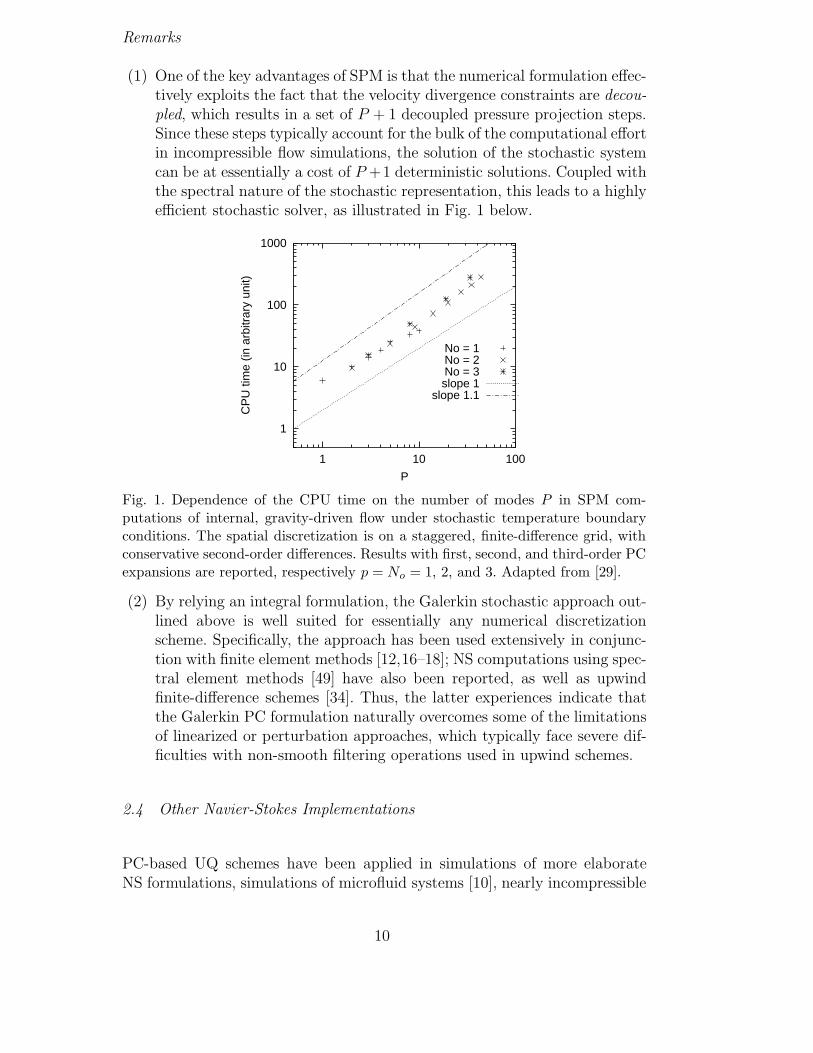
pled, which results in a set of P + 1 decoupled pressure projection steps.Since these steps typically account for the bulk of the computational effortin incompressible flow simulations, the solution of the stochastic systemcan be at essentially a cost of P +1 deterministic solutions. Coupled withthe spectral nature of the stochastic representation, this leads to a highlyefficient stochastic solver, as illustrated in Fig. 1 below.
1
10
100
1000
1 10 100
CP
U ti
me
(in a
rbitr
ary
unit)
P
No = 1No = 2No = 3slope 1
slope 1.1
Fig. 1. Dependence of the CPU time on the number of modes P in SPM com-putations of internal, gravity-driven flow under stochastic temperature boundaryconditions. The spatial discretization is on a staggered, finite-difference grid, withconservative second-order differences. Results with first, second, and third-order PCexpansions are reported, respectively p = No = 1, 2, and 3. Adapted from [29].
(2) By relying an integral formulation, the Galerkin stochastic approach out-lined above is well suited for essentially any numerical discretizationscheme. Specifically, the approach has been used extensively in conjunc-tion with finite element methods [12,16–18]; NS computations using spec-tral element methods [49] have also been reported, as well as upwindfinite-difference schemes [34]. Thus, the latter experiences indicate thatthe Galerkin PC formulation naturally overcomes some of the limitationsof linearized or perturbation approaches, which typically face severe dif-ficulties with non-smooth filtering operations used in upwind schemes.
2.4 Other Navier-Stokes Implementations
PC-based UQ schemes have been applied in simulations of more elaborateNS formulations, simulations of microfluid systems [10], nearly incompressible
10

Boussinesq flows [29], weakly compressible flow at low-Mach-number [28], re-acting flow [39], as well as fully compressible unsteady flow in a single spacedimension [33].
For brevity, we focus our attention on Galerkin approaches following the devel-opment outlined in section 2.2, and to multi-dimensional momentum solvers.Thus, we shall omit from the present discussion 1D compressible flow compu-tations [33], and reacting flow models [39]. Also omitted are stochastic sim-ulations of microfluidic systems [10], as the latter incorporate essentially thesame incompressible momentum update as in SPM [25,29].
An immediate, though non-trivial, generalization of the incompressible SPMconcerns weakly-compressible Boussinesq flows. This situation was consideredin [29], which focused on simulation of a stochastic variant of the coupledsystem:
∂u
∂t+ u · ∇u = −∇p +
Pr√Ra
∇2u + Prθy, (27)
∇ · u = 0, (28)
∂θ
∂t+ ∇ · (uθ) =
1√Ra
∇2θ. (29)
where θ is the normalized temperature, while Pr and Ra denote the Prandtland Rayleigh numbers, respectively. Generalization of the SPM outlined aboveto the case of Boussinesq flow is deemed immediate, since the major modifi-cations involve incorporation of the buoyancy source term in the momentumequation, and the simultaneous integration of an advection equation for tem-perature. The structure of the pressure projection steps, on the other hand,remains unchanged, as the presence buoyancy source terms only affects theirright-hand-sides. Thus, at least in the case of SPM, generalization from in-compressible to Boussinesq flow requires a straightforward adaptation of thestochastic scheme.
In contrast, generalization of stochastic incompressible NS solver to compress-ible zero-Mach-number flows can prove significantly more challenging. Such anexercise was considered in [28], which focused on extension of SPM to simula-tion of natural convection in a heated cavity under non-Boussinesq conditions.The simulations were based on a stochastic variant on the compressible NSequations in the zero-Mach-number limit [6, 32]:
∂ρ
∂t=−∇ · ρu (30)
∂(ρu)
∂t=−∂(ρu2)
∂x− ∂(ρuv)
∂y− ∂Π
∂x+
1√Ra
Φx (31)
11

∂(ρv)
∂t=−∂(ρuv)
∂x− ∂(ρv2)
∂y− ∂Π
∂y+
1√Ra
Φy −1
Pr
ρ − 1
2ε(32)
∂T
∂t=−u · ∇T +
1
ρPr√
Ra∇ · (κ∇T ) +
γ − 1
ργ
dP
dt(33)
P = ρT (34)
where ρ is the density, Π is the hydrodynamic pressure, Ra is the Rayleighnumber, ε is the temperature (Boussinesq) ratio, Φx and Φy are the viscousstress terms in the x and y directions, respectively, Pr is the Prandtl number,κ is the normalized thermal conductivity, γ is the specific heat ratio, and P (t)is the thermodynamic pressure [45].
As explained in [28], one delicate aspect of the generalization of SPM tozero-Mach-number flows concerns enforcement of the mass conservation con-straints. In the numerical scheme constructed in [28], these constraints leadto the following decoupled system of elliptic equations for the hydrodynamicpressure modes:
∇2Πk =1
∆t
∇ · (ρu)∗k +∂ρk
∂t
∣
∣
∣
∣
∣
n+1
, k = 0, . . . , P (35)
with homogeneous Neumann boundary conditions. These equations are thussubject to the following solvability constraints:
∫
Ω
1
∆t
∇ · (ρu)∗k +∂ρk
∂t
∣
∣
∣
∣
∣
n+1
dΩ = 0 (36)
In many situations, particularly in the case of a conservative discretization,the integral of the divergence term in Eq. (36) may be given as an integralover known boundary terms, and may thus be evaluated exactly. In particular,in the case of a domain bounded by stationary solid boundaries, the integralof the divergence term vanishes identically. On the other hand, the integralof the second term is significantly more delicate, because the density evolu-tion equation involves complex combinations of stochastic quantities which,generally, can only be approximately estimated. Consequently, without spe-cial care, the solvability constraints may only be approximately satisfied. Asexperienced in [28], this situation always led to unstable computations. Toovercome this difficulty, a special procedure for the evaluation of the globalmass conservation constraint was developed in [28]. The procedure ensuredthat solvability constraints were satisfied to machine precision, which resultedin a stable solver.
Note that in the case of a constant density flow, the time derivative in Eq. (36)
12

vanishes identically, while the integral of the divergence term also vanishes dueto the global mass (volume) conservation constraint (Eq. 14). Thus, unlike thecase of zero-Mach-number flow, for a conservative discretization the solvabil-ity conditions of the Poisson equations for the stochastic pressure modes areimmediately satisfied. Consequently, extensions of incompressible solvers tozero-Mach-number flows should include a suitable treatment of the mass di-vergence constraints.
13

3 PC computations
In this section we review some key concepts for the manipulation and imple-mentation of stochastic spectral expansions.
3.1 Quadratic products
In their simplest unreduced form, the unreduced NS equations involve quadratic(convective) non-linear terms. Consequently, the determination of the spectralexpansion of the quadratic product of the form c = ab, where a and b are givenby:
a(ξ) =P∑
i=0
aiΨi(ξ) and b(ξ) =P∑
j=0
bjΨj(ξ), (37)
is of primary interest. Applying the definition of the projection on the spectralbasis, we obtain the expression for the spectral coefficients of c, namely:
ck
⟨
Ψ2k
⟩
≡ 〈cΨk〉 = 〈(ab)Ψk〉 =P∑
i=0
P∑
j=0
aibj 〈ΨiΨjΨk〉 . (38)
Introducing the multiplication tensor Mijk defined in Eq. (20), Eq. (38) canbe rewritten as:
ck =P∑
i=0
P∑
j=0
Mijkaibj. (39)
The above convolution sum is a true Galerkin projection of c onto the subspacespanned by the Ψk, k = 0, . . . , P , but that higher-order terms, namely thoseinvolving polynomials of order > p are, of course, ignored. It is also interestingto note that, formally, Eq. (39) suggests that the operation count neededto determine a quadratic product is essentially O(P 3). However, due to thesparse nature of M, the operation count is actually much smaller. As furtherdiscussed in section 3.4, taking advantage of the “sparseness” of M is key forcomputational efficiency.
One can exploit Eq. (39) to derive expression for the PC expansion of theinverse of a stochastic quantity. Letting b denote the inverse of a, we have bydefinition:
(ab)k =∑
i
∑
j
Mijkaibj = δ0k (40)
14

where δ denote the Kronecker delta. Since the coefficients ai are known, theabove expression can be recast as a system of (P + 1) linear equations in theunknown coefficients bk, k = 0, . . . , P . A standard linear equation solver canthen be used to solve the system and hence determine the PC expansion of b.
3.2 Higher-order transformations
For many fluid problems of interest, the formulation involves complex physicalmodels requiring higher-order transformations of spectral quantities. A well-known example concerns reacting flows, where the governing equations includequadratic products as well as complex source terms involving higher-orderproducts, exponentiation, inversion, etc. . . These complex functionals requiresuitable spectral estimates, which, generally, may only constitute approximateGalerkin projections; balancing precision and computation cost is, in thesesituations, an important consideration.
3.2.1 Higher-order products
Consider first the ternary product d = abc. One can apply the same Galerkinprocedure used for quadratic products, which in the present case gives:
dl =P∑
i=0
P∑
j=0
P∑
k=0
Tijklaibjck (41)
where
Tijkl ≡〈ΨiΨjΨkΨl〉
〈ΨlΨl〉. (42)
Although T is also sparse, it has a significantly larger number of non-zeroentries than M, and Galerkin evaluation of d requires substantially higherstorage and CPU cost than a quadratic product. In order to reduce theserequirements, an alternative “pseudo-spectral” evaluation approach can beimplemented, based on successive application of the formula for quadraticproducts. For instance, d may be estimated using:
dk ≈∑
i
∑
j
(ab)icjMijk, where (ab)i =∑
m
∑
n
ambnMmni. (43)
15
The drawback of this approximate factorization is that it may introduce alias-ing errors. We also note that in general
∑
i
∑
j
(ab)icjMijk 6=∑
i
∑
j
(ac)ibjMijk 6=∑
i
∑
j
(bc)iajMijk, (44)
and so using the pseudo-spectral approach the spectral representation of ddepends on the order in which the approximate factorization is applied. How-ever, if the expansion order p is large enough, one may expect the resultingerrors to be small, as observed in actual computations. Also note that thesame factorization procedure can be applied to higher-order terms, writing forinstance abcd = [(ab)c]d.
3.2.2 Taylor series approach
Let f(a) denote a function of a stochastic quantity a with known PC repre-sentation. The Taylor expansion of f(a) about the mean of a = a0 is
f(a) = f(a0) +∞∑
l=1
(a − a0)l
l!f (l)(a0),
where f (l) = dlf/dal. If f is well behaved and the variance of a sufficientlysmall, one can expect the Taylor series to converge quickly with l. In thiscase, the series can be truncated after the first few terms, requiring only theestimation of the first powers of a ≡ a − a0 =
∑Pi=1 aiΨi, using for instance
the pseudo-spectral approach outlined above. However, if the Taylor seriesconverges slowly, the computation of the PC expansion of al, from al−1a, maybe plagued by significant errors as l increases, thus restricting the domain ofapplication for the Taylor series approach.
3.2.3 Simulation approach
A robust means for overcoming the limitation of the Taylor series approachconsists of avoiding approximation of higher powers, instead relying on sam-pling or simulation to directly determine the PC representation of f(a). Sincethe spectral coefficients fi of f(a) are by definition given by 〈f(a)Ψi〉 / 〈Ψ2
i 〉,one can apply the following sampling procedure to determine fi:
〈fΨi〉 ≈Ns∑
s=1
f(a(ξs))Ψi(ξs)w(ξs), (45)
where Ns is the number of samples, and (ξs, ws) are the sample points andassociated weights. Different sampling strategies can be used, including non-
16

deterministic sampling (e.g. Monte-Carlo, Latin hypercube, . . . ), quadrature,and cubature formulas (see section 4). It is emphasized that this approachonly requires the computation of f for different (deterministic) values of itsrandom argument a(ξ). The principal limitation of this simulation strategyconcerns the number of sample points Ns needed to achieve sufficient accuracy.Specifically, the computational cost may be prohibitively large in situationswhere a large value of Ns is needed to ensure small sampling errors.
3.3 Integration approach
This approach, recently introduced in [11], is based on differentiation of f ,followed by integration along a prescribed path. In the deterministic case,and provided that f can be differentiated, f(a) can be computed through theintegration of its derivative g(a) = df/da :
f(a) − f(a) =
a∫
a
gda,
where a is an arbitrary starting point where f can be evaluated. This ideacan be extended to the stochastic case as follow. First, consider the randomprocesses:
b = b(s, ξ) =P∑
i=0
bi(s)Ψi(ξ),
f = f(s, ξ) =P∑
i=0
fi(s)Ψi(ξ),
g = g(s, ξ) =P∑
i=0
gi(s)Ψi(ξ),
where s parametrized the integration path across the deterministic space ofPC coefficients, and g is still the derivative of f . The random process b(s, ξ) isarbitrary selected such that it evolves along the integration path from b = b(ξ)where f(b) can be easily evaluated, to b = a(ξ) at the end of the integration.
Assuming that b, f and g are analytic with respect to s, we have
s2∫
s1
∂f
∂sds =
s2∫
s1
g∂b
∂sds, (46)
and the result of the integration being path-independent. Equation (46) may
17
be rewritten as:
P∑
i=0
Ψi
s2∫
s1
dfi
dsds =
P∑
i=0
[fi(s2) − fi(s1)]Ψi =P∑
i=0
P∑
j=0
ΨiΨj
s2∫
s1
gi(s)dbj
dsds. (47)
Projecting onto the PC basis, we obtain for each index k :
fk(s2) = fk(s1) +∑
i
∑
j
s2∫
s1
Mijkgi(s)dbj
dsds. (48)
Then, given an integration path such that f(b(s1, ξ)) can be easily evaluated,and b(s2, ξ) = a(ξ), we obtain
fk(s2) =〈f(a)Ψk〉〈Ψ2
k〉= fk(s1) +
∑
i
∑
j
s2∫
s1
Mijkgidbj
dsds. (49)
In practice, the integration path from s1 to s2 is defined as:
b0(s) = a0,
bk(s) = aks − s1
s2 − s1
k > 0,(50)
such that fk(s1) = f(a0) for k = 0 and 0 for k > 0, and fk(s2) = fk(a).Then, the integration can be performed using standard techniques as long asthe spectral expansion of g, the derivative of f , can be computed along theintegration path.
Though the approach appears to have merely shifted the difficulty in evaluat-ing the PC expansion of f to that of its derivative, it still enables us to resolvea wide class of non-linear transformations, such as exponentials, logarithmsand powers of a [11]). Compared with the Taylor series approach, this integra-tion technique is more costly, due to multiple evaluations of the PC expansionsof g along the integration path. However, numerical tests have shown its effec-tiveness for situations with large variance of the argument, where applicationof the Taylor series approach is limited.
3.4 Computational strategies
An efficient implementation of PC expansions is a crucial step in conversion ofa deterministic code into a stochastic PC-based counterpart. In this section,
18
we provide here details on the so-called UQ-toolkit, which comprises a libraryof utilities that help streamline deterministic code conversions.
3.4.1 PC constructs
One of the key features in PC implementation concerns the tensor construc-tion of the multi-dimensional basis functions. For brevity, we illustrate theseconstructs using the classical Hermite-based PC expansions.
The multi-dimensional Hermite polynomials are constructed from tensor prod-ucts of the one-dimensional Hermite polynomials. Let Hi(ξ) denote the 1-DHermite polynomial of order i > 0 in ξ. Then the corresponding Ψi(ξ) is givenby:
Ψi(ξ) =n∏
j=1
Hα
(i)j
(ξj), (51)
where α(i) ≡ α(i)1 , . . . , α(i)
n is the multi-index of the polynomial Ψi. The order
of Ψi is pi =∑n
j=1 α(i)j . By convention, α(0) = 0, . . . , 0, so that Ψ0(ξ) = 1,
while the multi-indices for the first order polynomials are given by:
α(i) = 0, . . . , 0, α(i)i = 1, 0, . . . for i = 1, . . . , n, (52)
yielding Ψi=1,...,n = ξi. Polynomials with order 1 < pi ≤ p are typically de-termined by systematically “looping” over the various dimensions [23], andthis results in an ordered the representation of the Ψ′
is and the correspondingmulti-indices. The ordering scheme is in fact a key underlying feature of allPC operations.
3.4.2 Construction of the multiplication tensor
Determination of the multiplication tensor involves the evaluation of the ex-pectation of triple products of the form ΨiΨjΨk. Using the multi-index defi-nition, we have:
〈ΨiΨjΨk〉=
⟨(
n∏
m=1
Hα
(i)m
(ξm)
)(
n∏
m=1
Hα
(j)m
(ξm)
)(
n∏
m=1
Hα
(k)m
(ξm)
)⟩
=n∏
m=1
⟨
Hα
(i)m
Hα
(j)m
Hα
(k)m
⟩
, (53)
where we have made use of the statistical independence of the ξ’s. Equa-tion (53) shows that the multidimensional multiplication tensor can be de-
19
termined based on knowledge of the one-dimensional expectations 〈HiHjHk〉.The latter can be established using symbolic computations or tables (see forinstance [18]), or alternatively using the Gauss-Hermite quadratures [1, 23].Equation (53) also reveals the origin of the sparseness of M, as it is sufficientthat the 1-D expectation vanishes along one stochastic dimension to haveMijk = 0.
Taking advantage of the multi-index construction, only the non-zero entriesof the multiplication tensor are computed during a pre-processing stage, andstored using a sparse format for subsequent use in the computations.
3.5 UQ toolkit
Extension of a deterministic code to incorporate the PC representation of un-certainty consists of two elementary steps. First, all quantities and fields thatdepend on the uncertainty are extended to involve a supplementary index thatcorresponds to the single-index representation of the PC basis. The orderingscheme determined in the multi-index construct is also used for the presentpurpose. For instance, in a two-dimensional problem the deterministic discretevelocity uij, defined at the node (i, j) of a spatial mesh, is extended to uijk
where the two first indices still refer to the spatial location, while k refers tothe polynomial index. In other words, the uncertain velocity at node (i, j) hasfor expansion:
uij(θ) =∑
k
uijkΨk(ξ(θ)). (54)
After this index extension is implemented for all relevant variables, it is nec-essary to re-interpret all operations involving these quantities. Some of theseoperations are not affected by the uncertainty, as spatial differentiation forinstance, and need only to be repeated for all modes 0 ≤ k ≤ P . On theother hand, require a spectral treatment as discussed in this section 3.1. Asan example, consider the computation of the convective terms u∂u/∂x arisingin the momentum equation. In a first stage, we compute the spatial deriva-tives ∂ui/∂x = (∂xu)i for all modes. Then, in a second stage, the spectralcoefficients of the convective term, (u∂xu)k, are determined by applying themultiplication rule in (39), resulting in:
(u∂xu)k =∑
i
∑
j
Mijkui(∂xu)j. (55)
Note that the operations above involve local grid information, and so can beeasily and efficiently parallelized. Moreover, since the multiplication tensor is
20

sparse and stored in sparse format, it is advantageous to systematically relyon a subroutine that takes advantage of this feature. For instance in Fortran-like language, the spectral coefficients of the convective terms of our examplewould be obtained through
call prod(u,dudx,ududx)
where u and ududx are two arrays of length P + 1 containing the spectralcoefficients of u and ∂xu respectively, and prod returns the coefficients oftheir product in the array ududx. In a similar way, higher-order operationsare also implemented through systematic calls to subroutines contained in theUQ toolkit.
21

4 Non-intrusive formulations
In this section, we discuss an alternative to spectral computations which con-sists of performing the projection of the stochastic flow solution onto the spec-tral basis using a set of deterministic solutions. Since this approach does notrequire solution of the governing equations for the spectral modes, but needsonly the availability of a deterministic solver, it is termed “non-intrusive,” theterminology emphasizing the fact that modification of the deterministic solveris neither required nor performed. By construction, the non-intrusive approachcan also be qualified as a collocation method, as opposed to Galerkin method,since the projection is performed based on specific realizations or points in therandom parameter space. The non-intrusive alternative is especially attrac-tive in situations where one wants to propagate and quantify uncertainties ina complex problem using a deterministic code that should not be modified,for instance using commercial, legacy or certified codes. Another interestingfeature of the non-intrusive approach is that it naturally circumvents the dif-ficulties associated with the spectral treatment of high-order non-linearities.
As in the Galerkin method, the starting point of uncertainty quantification andpropagation in the non-intrusive context is the parametrization of the input-uncertainties. Again, we assume that the input random data are parametrizedusing a set of n independent and normalized Gaussian variables ξ(θ) = ξ1(θ), . . . , ξn(θ),and are interested, in particular, in the determination of the velocity modesuk, k = 0, . . . , P . The orthogonality of the spectral basis provides the followingexpressions for uk,
⟨
Ψ2k
⟩
uk = 〈u(ξ(θ))Ψk(ξ(θ))〉 =∫
u(ξ)Ψk(ξ)pdf(ξ)dξ, (56)
where, using the independence of the ξi’s,
pdf(ξ) =n∏
i=1
exp[−ξ2i /2]√
2π. (57)
Equation (56) shows that the velocity modes can be determined through thecomputation of the integrals on its right-hand side. Different means can beused to estimate these integrals, leading to the methods outlined below.
4.1 Stochastic methods
The first class of methods discussed here is based on stochastic sampling strate-gies. The simplest of these methods is the Monte-Carlo (MC) approach (see
22
e.g. [30]), which relies on an unbiased sampling of the random parameter space.In unbiased MC, The integrals are computed using:
∫
u(ξ)Ψk(ξ)pdf(ξ)dξ = limNmc→∞
1
Nmc
Nmc∑
m=1
u(ηm)Ψk(ηm), (58)
where the ηm are pseudo-random vectors, with independent components, gen-erated following the distribution of ξ given in Eq. (57). The flow has to besolved for each realization of the uncertain parameters, as prescribed by ηm.It is known that the convergence rate for unbiased sampling is 1/
√Nmc in the
asymptotic limit Nmc → ∞, so the precision of the MC projection method isinherently limited for large problems where the computation of individual real-izations are expensive. More complex (biased) stochastic sampling techniquescan be used to improve the convergence rate. There is a vast literature on im-provement of MC sampling strategies, including variance reduction techniques,stratified sampling, Latin-Hypercube sampling, and most of these techniquesare readily applicable to the integral in Eq. (56). In [29], we performed a non-intrusive numerical experiment for a natural convection flow inside a closedcavity, involving n = 6 uncertain parameters, and using a Latin-Hypercubesampler (LHS) [37]. The comparison with the Galerkin computation for thesame flow, clearly put in evidence the much lower efficiency of the LHS non-intrusive approach both in terms of CPU cost and accuracy. Note, however,that for problems with large number, n, of stochastic dimensions, the Galerkinapproach may face limitations due to memory requirements, while in con-trast the computation of individual realizations is insensitive to the numberof stochastic dimensions involved in the underlying uncertainty sources. Themain limitation of non-intrusive methods appears to be due to the number ofrealizations needed to properly sample the parameter space. Note also thatdifferent realizations of the flow are independent and can be computed on par-allel; for example, in [29] a 64-processor machine was used to take advantageof this feature.
4.2 Deterministic methods
In problems with a moderate number of stochastic dimensions, it may beadvantageous to apply a deterministic approach to compute the integrals inEq. (56), since deterministic methods usually exhibit greater flexibility in rateof convergence and accuracy control. This section discusses two possible de-terministic methods.
23
4.2.1 Gauss-type quadratures
For n = 1, Eq. (56) can be written as:
⟨
Ψ2k
⟩
uk =
+∞∫
−∞
u(ξ)Ψk(ξ)exp(−ξ2/2)√
2πdξ. (59)
Using the Gauss-Hermite (GH) quadrature formula [1], the integral can beestimated using the finite sum:
⟨
Ψ2k
⟩
uk ≈Nq∑
i=1
u(xi)Ψk(xi)wi, (60)
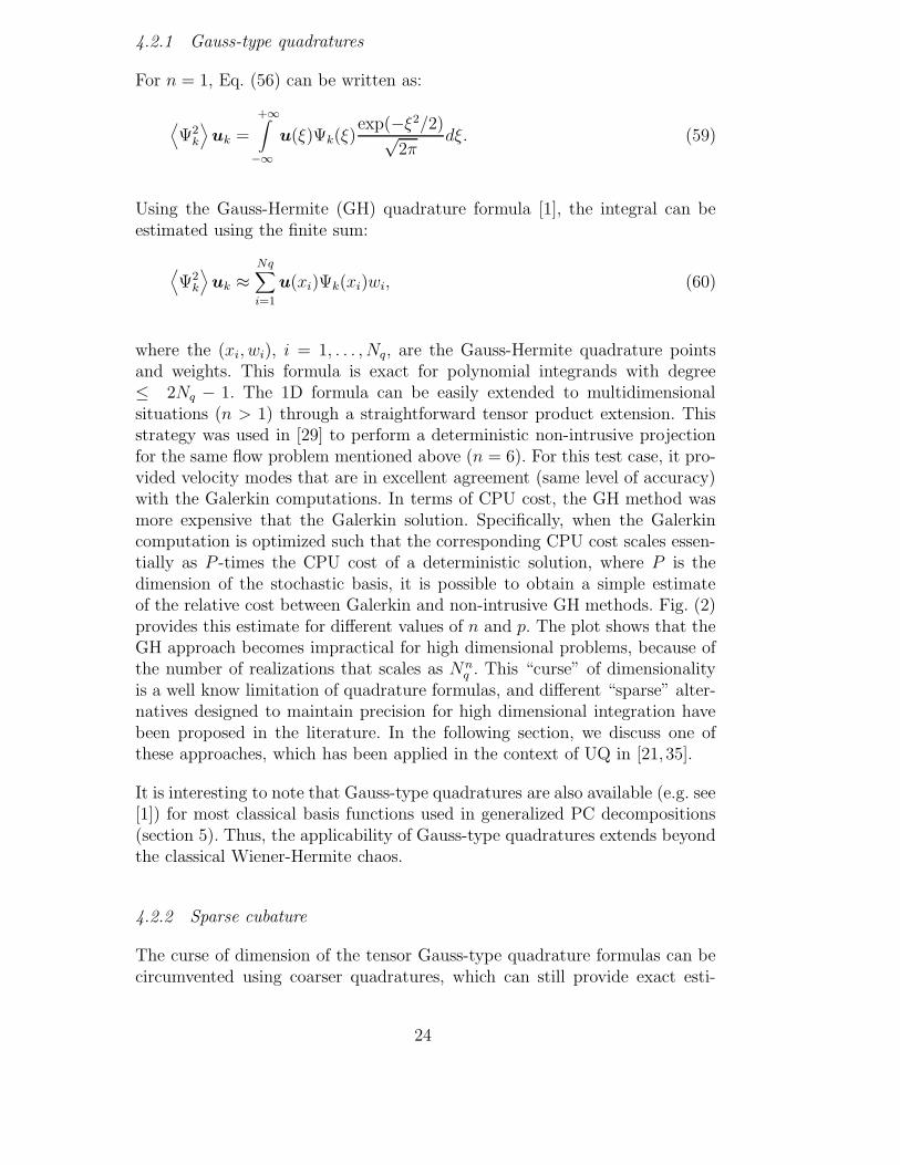
where the (xi, wi), i = 1, . . . , Nq, are the Gauss-Hermite quadrature pointsand weights. This formula is exact for polynomial integrands with degree≤ 2Nq − 1. The 1D formula can be easily extended to multidimensionalsituations (n > 1) through a straightforward tensor product extension. Thisstrategy was used in [29] to perform a deterministic non-intrusive projectionfor the same flow problem mentioned above (n = 6). For this test case, it pro-vided velocity modes that are in excellent agreement (same level of accuracy)with the Galerkin computations. In terms of CPU cost, the GH method wasmore expensive that the Galerkin solution. Specifically, when the Galerkincomputation is optimized such that the corresponding CPU cost scales essen-tially as P -times the CPU cost of a deterministic solution, where P is thedimension of the stochastic basis, it is possible to obtain a simple estimateof the relative cost between Galerkin and non-intrusive GH methods. Fig. (2)provides this estimate for different values of n and p. The plot shows that theGH approach becomes impractical for high dimensional problems, because ofthe number of realizations that scales as Nn
q . This “curse” of dimensionalityis a well know limitation of quadrature formulas, and different “sparse” alter-natives designed to maintain precision for high dimensional integration havebeen proposed in the literature. In the following section, we discuss one ofthese approaches, which has been applied in the context of UQ in [21, 35].
It is interesting to note that Gauss-type quadratures are also available (e.g. see[1]) for most classical basis functions used in generalized PC decompositions(section 5). Thus, the applicability of Gauss-type quadratures extends beyondthe classical Wiener-Hermite chaos.
4.2.2 Sparse cubature
The curse of dimension of the tensor Gauss-type quadrature formulas can becircumvented using coarser quadratures, which can still provide exact esti-
24
1 2
3 4
5 6
0 2
4 6
8 10
12
-6-5-4-3-2-1 0
log10 [CPUS / CPUNI]
pn
log10 [CPUS / CPUNI]
Fig. 2. Evolution with the number of stochastic dimensions n and expansion order p,of the ratio of CPUS, the CPU cost of the Galerkin computation (assuming a linearscaling with the basis dimension P + 1) with CPUNI the CPU cost of non-intrusiveprojection using the tensor Gauss-Hermite formula.
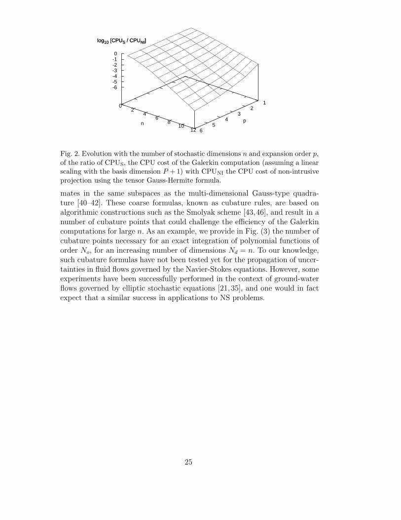
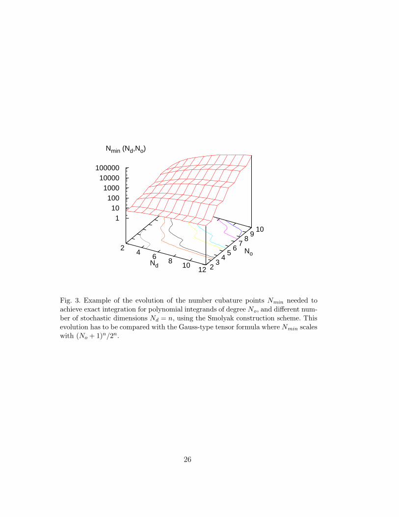
mates in the same subspaces as the multi-dimensional Gauss-type quadra-ture [40–42]. These coarse formulas, known as cubature rules, are based onalgorithmic constructions such as the Smolyak scheme [43,46], and result in anumber of cubature points that could challenge the efficiency of the Galerkincomputations for large n. As an example, we provide in Fig. (3) the number ofcubature points necessary for an exact integration of polynomial functions oforder No, for an increasing number of dimensions Nd = n. To our knowledge,such cubature formulas have not been tested yet for the propagation of uncer-tainties in fluid flows governed by the Navier-Stokes equations. However, someexperiments have been successfully performed in the context of ground-waterflows governed by elliptic stochastic equations [21, 35], and one would in factexpect that a similar success in applications to NS problems.
25
24
68
1012
Nd 23
45
67
89
10
No
110
1001000
10000100000
Nmin (Nd,No)
Fig. 3. Example of the evolution of the number cubature points Nmin needed toachieve exact integration for polynomial integrands of degree No, and different num-ber of stochastic dimensions Nd = n, using the Smolyak construction scheme. Thisevolution has to be compared with the Gauss-type tensor formula where Nmin scaleswith (No + 1)n/2n.
26

5 Generalized PC
Classical PC representations are based on a well-established theoretical foun-dation that takes advantage of the fact that the Hermite chaos is completeand orthogonal with respect to the Wiener measure [4]. In particular, Wiener-Hermite expansions are well suited when representing random data corre-sponding to Gaussian variables and processes.
Note, however, that it is possible to apply alternative orthogonal basis func-tions in PC expansions. This section outlines possible alternatives, and brieflyaddresses the question concerning their suitability and whether specific ad-vantages may be derived from their implementation. The discussion focusesexclusively on chaos decompositions corresponding to continuous measures,and considers separately the cases of local and global basis functions.
5.1 Global Basis Functions
A general construction that captures several possible choices of PC represen-tations is the so-called Wiener-Askey family, originally developed by Askeyand Wilson [3] and first introduced in the UQ context by Xiu and Karni-adakis [48]. In addition to the Hermite chaos, the Wiener-Askey family inparticular includes Laguerre and Jacobi basis functions. The latter are or-thogonal polynomials in random variables that follow gamma and beta distri-butions, respectively, orthogonality being naturally interpreted with respectto the corresponding measures.
From an implementation perspective, the computational framework of the UQtoolkit outlined above enables the user to navigate freely between differentbasis representations. Most of the effort associated with a change of basisconcerns the construction of the multiplication tensor(s), and procedures forother nonlinear transformations in case they are not based directly on thelatter. Thus, this effort is limited to pre- and post-processing, with little or nochange to the structure of the stochastic code. This is another key feature ofthe UQ toolkit.
It is also interesting to note, much like the Hermite case, PC representationsbased on the Laguerre and Jacobi polynomials are expected to exhibit expo-nential convergence as the order of the corresponding expansion is increased.Such convergence behavior is in fact guaranteed whenever certain smoothnessconditions are satisfied [5]. In such situations, selection of a specific basis func-tion representation would primarily be based on convenience, and to a lesserextent on the “efficiency” of the presentation –since the latter is generally notknown a priori.
27

In their original development [48], Xiu and Karniadakis provided several ex-amples in which the input random data have pdf’s that correspond to thoseof the random variables of basis functions belonging to Wiener-Askey chaos.They show through computational examples that it can be more advanta-geous to select a basis representation whose random variables have a similardistribution as the input random data. This is especially the case when thedistribution of the input data are such that exponential convergence is imme-diately lost when other basis function representations are selected.
On should note, however, that a rapidly convergent spectral representationof the input random data may not always constitute a key consideration inthe selection of a basis function representation. To support this assertion, oneobserves that PC representation generally provides a complete functional rep-resentation of the response of the stochastic solution in terms of the randomvariables. Specifically, one can readily determine particular solutions corre-sponding to specific realizations of the random variables. Consequently, hav-ing determined the response surface starting from given random input data,one can immediately determine the statistics of the solution for “new” ran-dom input having different statistics, so long as the new data “lives” on thesame portion of the probability space as the former. It should be emphasizedthat such transformation does not require that the solution be recomputedusing the new random input, as it can be readily determined using spectralprojections or alternatively via sampling or collocation. Sampling or colloca-tion approaches are quite suitable for this purpose, since the associated costsare, for most CFD problems of interest, substantially smaller than those re-quired to determine the original stochastic solution (in other words, for largenon-linear problems, the cost of uncertainty propagation is much larger thanthat of sampling the stochastic solution). Thus, it appears to the authors that,an approximate representation of random input data may, in many cases, beefficiently corrected in post-processing stages.
Beyond matters of computational convenience, and of representation of stochas-tic inputs, it is generally difficult to assess the impact of the basis functionrepresentation on the efficiency of the propagation computations. This is thecase because, for complex nonlinear problems, generally little is known a pri-
ori about the statistics of the solution, and the relationship between thesestatistics and those of the random inputs. On the other hand, if the statisticsof the solutions are known or constrained, one may attempt to take advantageof this knowledge by selecting a basis function representation that efficientlycaptures the known or constrained behavior, appropriately approximating therandom inputs using a few elements of this basis, and later correcting for theapproximation through post-processing.
An additional complication that has so far received little attention concernsthe case where the stochastic solution depends steeply or discontinuously on
28

the random inputs. In such situations, one would expect that a spectral rep-resentation in terms of global basis functions would exhibit severe difficulties.This topic is addressed in the section below, which shows that wavelet-baseddecompositions may be effective in addressing some of these difficulties.
5.2 Local Basis Functions
Uncertainty propagation may be especially challenging in cases where randominputs include critical parameters or bifurcation points. In such situations,the representation of the flow dependence on the uncertain parameters us-ing global polynomial basis may be impractical because of discontinuities orinsufficient smoothness along the stochastic dimensions. Specifically, the ex-ponential convergence rate may be lost, and Gibbs phenomena may resultin large errors or even global breakdown of the solution. To overcome thesedrawbacks, local expansions have been proposed in [26,27]. These expansionsuse Multi-Wavelets (see [2]) basis consisting in piece-wise continuous multidi-mensional polynomials.
For zero-order multi-wavelets (MW), one obtains a Wiener-Haar expansionwhich is a piece-wise constant approximation of the uncertain flow [26], i.e. itprovides local averages of the flow over sub-domains of the uncertain parameterspace, whose “volumes” are controlled by the resolution level. As the resolutionlevel increases, the flow is averaged over smaller and smaller portions of the pa-rameter space, thus allowing convergence to the exact response surface. In [26]an example is provided for the case of stochastic Rayleigh-Benard instabilityin a rectangular domain, the input uncertainty essentially corresponding to astochastic Rayleigh number which assumes both subcritical and supercriticalvalues. The numerical experiments showed that the (global) Wiener-Legendreexpansion was not able to converge to the correct solution, and that the oscil-latory character of the polynomials leads to unphysical predictions when theexpansion order is increased. On the other hand, the Wiener-Haar computa-tions provide robust estimates which converged towards the exact stochasticsolution as the number of refinement levels increased.
The improvement in robustness and stability provided by MW expansions isachieved at the cost of a lower convergence rate, the stochastic errors nowbeing controlled by the polynomial order (p-convergence) and the refinementlevel (h-convergence). Also the dimension of the spectral basis dramaticallyincreases with the resolution level and polynomial order, especially for prob-lems with a large number of stochastic dimensions n. However, the commonsituation concerns a smooth dependence of the flow over large portions of theparameter space, where high-order expansions are well suited, separated bylocalized steep/discontinuous variations, where the robustness of low order
29

expansions highly desired. Thus, an optimal, non-global representation wouldinvolve high-order polynomial expansions over large sub-domains of the pa-rameter space, where p-convergence is attractive, and low-order expansions inregions of steep/discontinuous variation, where h-convergence is highly effec-tive. This ideal picture is similar to the spatial spectral-element discretizationsstrategies, the discretization being now implemented in the space of randomdata. Since the behavior of the stochastic solution is generally not known a pri-
ori, an adapted mesh of the parameter space can not be determined before thecomputations are performed. Thus, automatic refinement strategies are soughtin order to tune the local resolution level and the polynomial order. Most ofthe techniques developed for Automatic Mesh Refinement (AMR) can in prin-ciple be applied or adapted for the present purpose. For instance, in [27] anautomatic procedure, involving an a priori error estimator based on the localMW expansion, was designed to determine the need for local stochastic re-finement. Compared to spatial AMR techniques, one observes that refinementof the random parameter space is easier to handle since solutions over sub-domains can be obtained independently. This features substantially simplifiesdata management, and allows for straightforward parallel implementations.
30
6 Outlook
As highlighted above, various implementations of PC representations havebeen recently applied to the development of stochastic NS solvers. These de-velopments have been in large part motivated by the promise of achievingaccurate representations of the impact of uncertain input data, at efficiencylevels that far exceed those of MC computations. This review has, in particu-lar, identified various areas of recent progress.
The use of PC-based representations for stochastic NS computations is stilla developing field. There is, consequently, a large potential for substantialadvances. Based our own recent experiences –and consequently biases– weconclude with a brief outline of some of the corresponding opportunities andchallenges:
(1) The development of flexible and robust computational libraries for accu-rate and efficient evaluation of PC transformation can be regarded as anessential tool for the construction of stochastic PC-based stochastic codes.Briefly, these libraries have enabled efficient transformation of determin-istic codes into stochastic codes. This transformation, however, requiresuser intervention, primarily to replace deterministic operations with thecorresponding functional calls into the stochastic library. An interestingconcept worth pursuing consists of an “automating” transformation, inwhich deterministic operations would be replaced by stochastic counter-parts at essentially compilation or during run time. The developmentof software tools that would enable such key capabilities appears to bepresent a key opportunity that would benefit and accelerate a wide rangeof investigations.
(2) One of the challenges facing PC representations arises in situations inwhich both the deterministic and stochastic systems exhibit limit cycleoscillations (LCO). To illustrate these challenges, on can consider theidealized case of a linear oscillator having a random, say Gaussian, fre-quency. The exact solution of such an idealized system, which can bereadily determined, indicates that at large time the solution exhibits arandom phase that is uniformly distributed over the unit circle. An im-mediate dilemma facing such situations concerns the selection of a basis,as those based on continuous random variables generally face severe dif-ficulties in providing efficient representations of both the input and theoutput. Much needed are robust means to overcome such difficulties.
(3) Another set of challenges concerns situations where one is only interestedin assessing the impact of uncertainty on specific observables or compo-nents of the solution. These are in many ways akin to the problems justmentioned. For instance, in problems admitting LCOs, one may only beinterested in stochastic amplitudes and frequencies, but not in relating
31

the phase of different stochastic realizations. The development of compu-tational PC methods enabling such “projections” appears to be a worthyendeavor.
(4) Computational experiences obtained using PC representations in un-steady NS computations have so far been quite encouraging. In partic-ular, efficient schemes have been developed exhibiting superior conver-gence characteristics. On the other hand, theoretical results concerningthe behavior of the systems of stochastic equations resulting from PCrepresentations of stochastic NS equations are lacking. Of particular in-terest would be the pursuit of rigorous results concerning the stability ofsuch systems of stochastic equations and, if necessary, numerical methodsto stabilize the corresponding computations.
(5) Recent experiences with wavelet-based decompositions in stochastic NScomputations have pointed to the potential of constructing highly-efficient,accurate and robust UQ schemes. While experiences gained so far arequite limited, they indicate the promise of local refinement techniques aswell as adaptive order methods in which the order of PC expansions isalso adapted together with local refinement of random parameter space.These methods are yet to be fully exploited in the context of stochasticNS computations.
Finally, we recall that the development UQ methods for CFD computationshas in many cases been motivated by the increasingly-elaborate, underlyingphysical models, typically including a large number of uncertain parameters.The impact that UQ schemes can bring to such situations is in large part con-ditioned on a suitable representation of the uncertainty in the model inputs.Though the issue of representation of uncertain inputs has not been centralto the present review, it should evidently not be overlooked during implemen-tations. This may represent an especially delicate task in the case of complexmodels, which may incorporate uncertain, possibly correlated, data gatheredfrom different experiments, observations and/or simulations.
32
Acknowledgments
The authors acknowledge helpful interactions with collaborators, particularlyR. Ghanem, H. Najm, B. Debusschere, and M. Reagan. This work was sup-ported by the Laboratory Directed Research and Development Program atSandia National Laboratories, by the Defense Advanced Research ProjectsAgency (DARPA) and Air Force Research Laboratory, Air Force MaterielCommand, USAF, under agreement number F30602-00-2-0612. The U.S. gov-ernment is authorized to reproduce and distribute reprints for Governmentalpurposes notwithstanding any copyright annotation thereon. Computationswere performed at the National Center for Supercomputer Applications. OKalso acknowledges support from the Alexander von Humboldt Foundation.
33

References
[1] M. Abramowitz and I.A. Stegun. Handbook of Mathematical Functions. Dover,1970.
[2] B.K. Alpert. A class of bases in L2 for the sparse representation of integraloperators. SIAM J. Math. Anal., 24:246–262, 1993.
[3] R. Askey and J. Wilson. Some basic hypergeometric polynomials that generalizeJacobi polynomials. Mem. Amer. Math. Soc., 319, 1985.
[4] R.H. Cameron and W.T. Martin. The orthogonal development of nonlinearfunctionals in series of Fourier-Hermite functionals. Ann. Math., 48:385–392,1947.
[5] C. Canuto, Y. Yousuff Hussaini, A. Quasteroni, and T.A. Zang. Spectral
Methods in Fluid Dynamics. Springer-Verlag, 1988.
[6] D. Chenoweth and S. Paolucci. Natural convection in an enclosed vertical layerwith large horizontal temperature differences. J. Fluid Mech., 169:173–210,1986.
[7] A.J. Chorin. A numerical method for solving incompressible viscous flowproblems. J. Comput. Phys., 2:12–26, 1967.
[8] A.J. Chorin. Gaussian fields and random flow. Journal of Fluid Mechanics,63:21–32, 1974.
[9] S.C. Crow and G.H. Canavan. Relationship between a Wiener-Hermiteexpansion and an energy cascade. Journal of Fluid Mechanics, 41:387–403,1970.
[10] B. Debusschere, H.N. Najm, A. Matta, O.M. Knio, R.G. Ghanem, andO.P. Le Maıtre. Protein labeling reactions in electrochemical microchannelflow: Numerical prediction and uncertainty propagation. Physics of Fluids,15(8):2238–2250, 2003.
[11] B.J. Debusschere, H.N. Najm, P.P. Pebray, O.M. Knio, R.G. Ghanem, and O.P.Le Maıtre. Numerical challenges in the use of Polynomial Chaos representationsfor stochasic processes. SIAM J. Sci. Comp., 2004. in press.
[12] R. Ghanem. Ingredients for a general purpose stochastic finite elementformulation. Computer Methods in Applied Mechanics and Engineering, 168:19–34, 1999.
[13] R. Ghanem and S. Dham. Stochastic finite element analysis for multiphase flowin heterogeneous porous media. Transport in Porous Media, 32:239–262, 1998.
[14] R.G. Ghanem. Probabilistic characterization of transport in heterogeneousmedia. Computer Methods in Applied Mechanics and Engineering, 158:199–220, 1998.
34

[15] R.G. Ghanem and O.M. Knio. A probabilistic framework for the validation andcertification of computer simulations. In Proceedings of 1st JANNAF Modeling
and Simulation Subcommittee Meeting, 2000.
[16] R.G. Ghanem and R.M. Kruger. Numerical solution of spectral stochastic finiteelement systems. Computer Methods in Applied Mechanics and Engineering,129:289–303, 1996.
[17] R.G. Ghanem and P.D. Spanos. A spectral stochastic finite element formulationfor reliability analysis. J. Eng. Mech. ASCE, 117:2351–2372, 1991.
[18] R.G. Ghanem and P.D. Spanos. Stochastic Finite Elements: A Spectral
Approach. Springer Verlag, 1991.
[19] T.D. Hien and M. Kleiber. Stochastic finite element modeling in linear transientheat transfer. Computer Methods in Applied Mechanics and Engineering,144:111–124, 1997.
[20] G. Kallianpur. Stochastic Filtering Theory. Springer-Verlag, 1980.
[21] A. Keese and H. G. Matthies. Sparse quadrature as an alternative toMonte Carlo for stochastic finite element techniques. Proceedings in Applied
Mathematics and Mechanics, 3(1):493–494, 2003.
[22] J. Kim and P. Moin. Application of a fractional-step method to incompressiblenavier-stokes equations. J. Comput. Phys., 59:308–323, 1985.
[23] O.M. Knio and R.G. Ghanem. Polynomial Chaos product and momentformulas : A user utility. Technical report, The Johns Hopkins University,Baltimore, MD, to appear.
[24] O.P. Le Maıtre, O.M. Knio, B.D. Debusschere, H.N. Najm, and R.G. Ghanem.A multigrid solver for two-dimensional stochastic diffusion equations. Computer
Methods in Applied Mechanics and Engineering, 92(41-42):4723–4744, 2003.
[25] O.P. Le Maıtre, O.M. Knio, H.N. Najm, and R.G. Ghanem. A stochasticprojection method for fluid flow. i. basic formulation. Journal of Computational
Phyics, 173:481–511, 2001.
[26] O.P. Le Maıtre, O.M. Knio, H.N. Najm, and R.G. Ghanem. Uncertaintypropagation using Wiener-Haar expansions. Journal of Computational Phyics,197(1):28–57, 2004.
[27] O.P. Le Maıtre, H.N. Najm, R.G. Ghanem, and O.M. Knio. Multi-resolution analysis of Wiener-type uncertainty propagation schemes. Journal
of Computational Phyics, 197(2):502–531, 2004.
[28] O.P. Le Maıtre, M.T. Reagan, B. Debusschere, H.N. Najm, R.G. Ghanem,and O.M. Knio. Natural convection in a closed cavity under stochastic, non-Boussinesq conditions. SIAM J. Sci. Comput., 2004. in press.
[29] O.P. Le Maıtre, M.T. Reagan, H.N. Najm, R.G. Ghanem, and O.M. Knio.A stochastic projection method for fluid flow. ii. random process. Journal of
Computational Phyics, 181:9–44, 2002.
35

[30] J.S. Liu. Monte Carlo Strategies in Scientific Computing. Springer Verlag, 2001.
[31] M. Loeve. Probability Theory. Springer, 1977.
[32] A. Majda and J. Sethian. The derivation and numerical solution of the equationsfor zero-Mach number combustion. Comb. Sci. and Technology, 42:185–205,1985.
[33] L. Mathelin, M.Y. Hussaini, T.A. Zang, and F. Bataille. Uncertaintypropagation for turbulent compressible flow in a quasi-1d nozzle using stochasticmethods. AIAA Journal, 2004. in press.
[34] A. Matta. Numerical Simulation and Uncertainty Quantification in Microfluidic
systems. PhD thesis, Department of Civil Engineering, Johns HopkinsUniversity, 2003.
[35] H. Matthies and A. Keese. Galerkins methods for linear and nonlinearelliptic stochastic partial differential equations. Report 2003-08, Inst.Scientific Computing, Technical University Braunschweig, Technical UniversityBraunschweig Brunswick, Germany, 2003.
[36] H.G. Matthies, C.E. Brenner, C.G. Bucher, and C.G. Soares. Uncertaintiesin probabilistic numerical analysis of structures and solids - stochastic finite-elements. Structural Safety, 19(3):283–336, 1997.
[37] M. McKay, R. Beckman, and W. Conover. A comparison of three methods forselecting values of input variables in the analysis of output from a computercode. Technometrics, 21(2):239–245, 1979.
[38] W.C. Meecham and D.T. Jeng. Use of the Wiener-Hermite expansion for nearlynormal turbulence. Journal of Fluid Mechanics, 32:225, 1968.
[39] H.N. Najm, M.T. Reagan, O.M. Knio, R.G. Ghanem, and O.P. Le Maıtre.Uncertainty quantification on reacting flow modelling. Technical Report 2003-8598, SANDIA, 2003.
[40] E. Novak and K. Ritter. High-dimensional integration of smooth functions overcubes. Numerische Mathematik, 75:79–97, 1996.
[41] E. Novak and K. Ritter. The curse of dimension and a universal method fornumerical integration. In G. Nurnberger, J. W. Schmidt, and G. Walz, editors,Multivariate Approximation and Splines, ISNM, pages 177–188. Birkhauser,Basel, 1997.
[42] E. Novak and K. Ritter. Simple cubature formulas with high polynomialexactness. Constructive Approximation, 15:499–522, 1999.
[43] K. Petras. Fast calculation of coefficients in the Smolyak algorithm. Numerical
Algorithms, 26:93–109, 2001.
[44] B.D. Phenix, J.L. Dinaro, M.A. Tatang, J.W. Tester, J.B. Howard, andG.J. McRae. Incorporation of Parametric Uncertainty into Complex KineticMechanisms: Application to Hydrogen Oxidation in Supercritical Water.Combustion and Flame, 112:132–146, 1998.
36
[45] P. Le Quere, R. Masson, and P. Perror. A Chebychev collocation algorithm for2d non-Boussinesq convection. J. Comput. Phys., 103:320–334, 1992.
[46] S.A. Smolyak. Quadrature and interpolation formulas for tensor products ofcertain classes of functions. Dokl. Akad. Nauk SSSR, 4:240–243, 1963.
[47] S. Wiener. The Homogeneous Chaos. Amer. J. Math., 60:897–936, 1938.
[48] D.B. Xiu and G.E. Karniadakis. The Wiener-Askey Polynomial Chaos forstochastic differential equations. SIAM J. Sci. Comput., 24:619–644, 2002.
[49] D.B. Xiu and G.E. Karniadakis. Modeling uncertainty in flow simulations viageneralized Polynomial Chaos. Journal of Computational Physics, 187:137–167,2003.
37