uncertainty evaluation of reservoir simulation models using particle swarms and hierarchical
TRANSCRIPT

Uncertainty Evaluation
of Reservoir Simulation Models using
Particle Swarms and Hierarchical Clustering
Muhammad KathradaMuhammad KathradaMuhammad KathradaMuhammad Kathrada
Submitted for the
Degree of Doctor of Philosophy
Institute of Petroleum Engineering
Heriot-Watt University
June 2009
This copy of the thesis has been supplied on condition that anyone who consults it is understood
to recognize the copyright rests with its author and that no quotation from the thesis and no
information derived from it may be published without the prior written consent of the author or the
University (as may be appropriate).

2
Abstract
History matching production data in finite difference reservoir simulation
models has been and always will be a challenge for the industry. The
principal hurdles that need to be overcome are finding a match in the first
place and more importantly a set of matches that can capture the uncertainty
range of the simulation model and to do this in as short a time as possible
since the bottleneck in this process is the length of time taken to run the
model. This study looks at the implementation of Particle Swarm
Optimisation (PSO) in history matching finite difference simulation models.
Particle Swarms are a class of evolutionary algorithms that have shown
much promise over the last decade. This method draws parallels from the
social interaction of swarms of bees, flocks of birds and shoals of fish.
Essentially a swarm of agents are allowed to search the solution hyperspace
keeping in memory each individual’s historical best position and iteratively
improving the optimisation by the emergent interaction of the swarm. An
intrinsic feature of PSO is its local search capability. A sequential niching
variation of the PSO has been developed viz. Flexi-PSO that enhances the
exploration and exploitation of the hyperspace and is capable of finding
multiple minima. This new variation has been applied to history matching
synthetic reservoir simulation models to find multiple distinct history

3
matches to try to capture the uncertainty range. Hierarchical clustering is
then used to post-process the history match runs to reduce the size of the
ensemble carried forward for prediction.
The success of the uncertainty modelling exercise is then assessed by
checking whether the production profile forecasts generated by the ensemble
covers the truth case.

4
Acknowledgements
I would like to thank the Herriot-Watt Uncertainty Joint Industry Program
for funding of this work, the sponsors being BG, BP, Chevron, ConocoPhillips,
DTI, JOGMEC, Hydro, ENI, Shell & Transform. At Shell, I’d like to thank
Dick Eikmans, whom it was always great to bounce ideas off.

5
Contents
1 Introduction 7
1.1. Introduction to Numerical Reservoir Simulation 11
1.2. A Brief History of History Matching 18
1.3. General History Matching Approaches 24
1.4. Swarm Intelligence 35
2 Review of Particle Swarm Optimisation 39
2.1. Background to Particle Swarms 39
2.2. The Canonical PSO 42
2.3. The Inertia Weight PSO 43
2.4. The Constriction Factor PSO 47
2.5. Parameter Sensitivities 48
3 Development of a new Particle Swarm Variant 53
3.1. The Flexi-PSO 53
3.2. Qualitative Behaviour of the Swarm 64
3.3. Sequential Niching 72
3.4. Function Stretching 81
3.5. Handling Mixed Integer Problems 86
4 Mathematical testing of the Flexi-PSO 89
4.1. CEC 2005 benchmark test set 89
4.2. Neural network model of the IRIS dataset 98
4.3. Integer Problems 107
5 Hierarchical Clustering 109
5.1. Agglomerative Hierarchical Clustering 109
5.2. Clustering the IRIS dataset 114

6
6 History Matching & Forecasting : Case Study of the Imperial
College Fault Model 116
6.1. Low Discrepancy Sequences 117
6.2. Model Definition 120
6.3. Results and Discussion 123
7 History Matching & Forecasting : Case Study of a North Sea Gas Field 139
7.1. Field Description 140
7.2. Results and Discussion 146
8 Conclusions 159
Appendix 166
Appendix A : CEC 2005 Mathematical Function Set 167
Appendix B : IRIS Dataset 200
Bibliography 204

Chapter 1 Introduction
7
Chapter 1
Introduction
Although much attention is focussed on new oil and gas developments, more
than 70% of the worlds production comes from fields that are more than 30
years old. Maturing reservoirs come with a unique set of management
challenges, from increased water cuts and gas-oil ratios through to aging
technologies and health and safety implications. An added challenge to these
reservoirs is that they often require more detailed forecasts of production
behaviour, even though production volumes and hence revenues are lower.
With the importance of understanding and forecasting the production
increasing as well as the oil and gas becoming more difficult to extract,
production costs also rise.
This leads to searching for an effective tool that can predict production
behaviour. Reservoir simulation is one of the principal tools employed in the
oil and gas industry to develop oil and gas bearing formations. This tool is
used to evaluate different field development/management options against one
another and thus maximise the economic value of the project. For the
simulation model to be of any value, it needs to be representative of the
subsurface structure, rock and fluid properties. For fields that have already

Chapter 1 Introduction
8
been on production, the engineer can use the historical production data in an
inverse manner to calibrate uncertain geological/fluid-flow parameters in the
simulation model. This process of adjusting the reservoir model until it
closely reproduces its past behaviour is typically referred to as “history
matching”, and is probably the number one topic of interest within the
reservoir simulation community. History matching also plays a key role in
developing an integrated approach to reservoir management because it
allows the static geological model to be rationalised with production data.
Initially the objective of the history match study needs to be defined. The
objective is mainly driven by the underlying business decision process in
reservoir management e.g. reservoir planning, infill drilling campaigns,
decisions on EOR incremental reserves, platform requirements, investigation
of the impact of subsurface uncertainties on the reserves etc.
Multiple solutions exist to the history matching problem i.e. different history
matched simulation models may not differ in the quality of their match
criteria, but they may produce different results in the forecasting stage. This
model diversity provides a basis for the quantification of uncertainties related
to production forecasts and the estimation of the remaining reserves of a
producing field.

Chapter 1 Introduction
9
Quite often the history matching process is undertaken deterministically
where the engineer defines a set of reservoir / well parameters and some
sensible ranges through which these parameters can be varied. He then goes
through a tedious trial and error process varying these parameters, often one
at a time to gain a sensitivity of the effect of that parameter on the system,
analyse the results on completion of each run and then try some other
combination of parameters that he intuitively feels would result in a lower
error between the simulated and the historical data. This can often take
many months, the outcome of which is not certain to yield a decent match at
all particularly if the field is large and there are complex mechanisms at play
within the reservoir.
In addition there is no guarantee that the match would be able to predict
future reservoir performance either, which is why an ensemble of matches
would give a better idea of what the prediction range may be. The
shortcoming of the deterministic method is that the human brain can hardly
visualise in more than four dimensions and most field history matches have
many parameters that can be varied. With such a large number of unknown
parameters to consider, traditional manual history matching remains very
much a work in progress.

Chapter 1 Introduction
10
There are technological developments in both history matching and reservoir
simulation that are helping to address today’s reservoir management
challenges. The rise of computer assisted history matching is an example of
this. Computer assisted history matching allows the engineer to focus on
developing an understanding of reservoir mechanisms and their relative
impact on production behaviour. Through such tools, match modifiers are
updated intelligently to try to increasingly improve the history match. It also
makes it possible to consider more information when developing a history
match or sensitising an appraisal. With manual history matching it can be
impossible to evaluate all aspects of the reservoir description that could have
an effect on the reservoir behaviour.
With computer assisted history matching however, large numbers of
modifiers can be evaluated in a full physics simulator and in fewer runs to
provide multiple matches of the reservoir to the production history. The
results are then used with the simulator to predict how a field will perform
and give measures of the uncertainty of these predictions. This in turn leads
to valuable information on the economics of the reservoir.
This thesis addresses the area of assisted history matching where an
algorithm is devised to search the hyperspace, and be quicker than a human
at finding combinations of the uncertain parameters that would match the

Chapter 1 Introduction
11
historical production data. We begin with a brief journey through the Society
of Petroleum Engineers (SPE) literature to put into perspective the various
approaches that have been used over the years and where the proposed
methodology fits in. It is also to delineate the key advantages and
disadvantages of the various methodologies. The Particle Swarm
Optimisation method and its performance on benchmark mathematical
functions, training a feed-forward neural network model and integer
problems will be discussed. Then the Flexi-PSO will be tested on the Imperial
College Fault Model that is widely regarded as a benchmark test case for
history matching due to its difficult fitness landscape. The Flexi-PSO is then
used to history match a synthetic version of a real North Sea gasfield model.
1.1. Introduction to Numerical Reservoir Simulation
Numerical reservoir simulation is the mathematical replication of the real
physical processes of fluid flow that occur within oil and gas reservoirs
(Ertekin et al, 2001). It is a model that represents the reservoir by a set of
mathematical equations derived from first principles of flow through porous
media. These equations can be solved analytically or numerically. As is so
often found in engineering systems, the model can require assumptions to
simplify the problem statement. If however, there are too many simplifying

Chapter 1 Introduction
12
assumptions or the simplifying assumptions deviate too far from the true
physics of the system, then the simulation can lead to unreliable results.
A reservoir simulation model is typically composed of a representation of the
reservoir as well as a set of equations describing fluid flow through the
reservoir. The reservoir representation begins with the geophysics discipline
where the boundaries of the reservoir are demarcated. This is followed by the
geology and petrophysics disciplines that determine the content of this
demarcated volume. This volume is then populated by a geological model
which could be a river channels, turbidite systems, etc. This geological model
then uses information from wells which have been drilled as well as seismic
data from the geologist to populate a set of rock parameters within this
volume.
This geological model is discretised into a grid of blocks or cells as they are
commonly known. An example of this is shown in Figure 1.1. This figuire
shows a reservoir grid with wells penetrating the gridblocks at locations
where they are in reality. Each gridblock has an associated set of reservoir
rock properties that represents the volume that the gridblock is associated
with. These properties can change with time as the reservoir undergoes
production and injection, however the model is initialised with properties as
found when initially drilled.

Chapter 1 Introduction
13
Figure 1.1. Example of a reservoir simulation grid
Typically the following data is required for any simulation model (Koederitz,
2005) :-
A. Gridblock location dependent parameters
• Location of each gridblock node in space viz. x, y, z co-ordinate
• Net to Gross (that amount of rock volume which can allow fluid
flow)
• Effective Porosity (ϕ) – the ratio of connected void space to bulk
volume of the rock
• Absolute permeability in each direction viz. kx, ky and kz. This
determines the speed of fluid flow through the reservoir rock.
W3 W4
W2
W5
W1
N

Chapter 1 Introduction
14
• Pressure (P) expected over the gridblock volume
• Phase saturations typically oil, water and gas (So, Sw & Sg).
However if enhanced oil processes are being undertaken,
additional liquid and/or solid phases could be present)
B. Saturation dependent properties
• Capillary pressue (Pc) is the difference in pressure across the
interface of two immiscible fluid phases. This is used to initialise
the saturation profile of the various phases in the reservoir
simulator
• Relative permeability (kro, krw & krg) is the measurement of the
ability of two or more fluid phases to pass through a formation
matrix. When more than phase is present in the reservoir rock,
each phase tends to inhibit the flow of the other. Relative
permeability (kr) is multiplied by absolute permeability (k) to
give an effective permeability (ke) for each phase flow
C. Fluid and Rock parameters which are pressure dependent
• Formation volume factors of oil, water and gas (Bo, Bw and Bg)
which is the ratio of a unit volume of reservoir fluid to the
volume it would occupy at standard conditions (1 atm, 60 °F) at
the surface

Chapter 1 Introduction
15
• Gas-Oil Ratio (Rs) which is the ratio of the volume of gas
dissolved in the oil to the volume of oil itself at standard
conditions
• Densities of each fluid phase viz. oil, water and gas (ρo, ρw & ρg)
• Viscosities of each fluid phase (µo, µw & µg)
• Fluid (oil, water and gas) and Rock Compressibilities (co, cg, cw &
cf). This is a measure of the change in volume of the fluid and
rock with a change in pressure
D. Well and Surface Facilities data
• Location of perforations of each well in the grid co-ordinate
system. This is important as these gridblocks act as pressure
sinks for the movement of fluid from other parts of the reservoir
• Production and injection data comprising of phase rates and
pressure when history matching
• Production and injection constraints due to facilities handling
limits and pressure drawdown constraints on the wells when
forecasting
The reservoir simulator uses all the above data in a set of mathematical
equations to describe the simultaneous fluid flow of multiple phases as well
as transfer of mass between the phases (usually between oil and gas) in the

Chapter 1 Introduction
16
reservoir. The equations essentially describe the interaction between gravity,
viscous and capillary forces within the porous media. Darcy’s Law is the basis
of these fluid flow equations which when applied to multiple phases over time
is formulated as partial differential equations which are solved numerically
in the simulator.
Darcy’s Law is based on experimental work done by a civil engineer Henry
Darcy in1856 on the water filtration systems in Dijon, France. In 1-
dimension and for linear flow for a fluid with viscosity µ, his law expounds
that in a horizontal plane the volumetric flow rate, q, through a porous
medium of length L and cross-sectional area A (Figure 1.2) is given by the
following equation (1.1.1) :-
( )L
PPkAq inout
µ
−−= (1.1.1)
Figure 1.2. Diagram of Darcy’s Experiement
k (permeability) in this equation is a derived property since all the other
parameters are experimentally known. The equation can be formulated in the

Chapter 1 Introduction
17
x, y and z directions by introducing pressure gradient and directional
permeability tensor terms.
The equations used in the reservoir simulator are derived from Darcy’s Law
that honour the mass balance between flow for each phase through adjacent
gridblocks and from gridblocks into wells and hence give the saturation and
pressure changes at any spatial point in the reservoir with time. The
equations are complex nonlinear partial differential equations which are
difficult to solve analytical and typically numerical methods are used. Finite
difference techniques are used to discretise the reservoir model in space and
time. The equations then need to be linearised and can be solved explicitly or
implicitly. Explicitly means that gridblock, fluid, rock and saturation
dependent parameters are updated at the end of every timestep with the
calculated pressure whereas Implicit schemes solve all the parameters
including pressure simultaneously at the end of the timestep. Usually a
direct or an iterative technique e.g. Newtons method is used to solve the
system of linearised equations.
Simulation models with a large number of gridblocks can take quite long to
simulate particularly if a detailed fluid model using an Equation of State is
required. An Equation of State is a rigourous thermodynamic representation
of the reservoir fluid at any pressure and temperature (Whitson et al, 2000).

Chapter 1 Introduction
18
The reservoir simulator now needs to solve an additional set of
thermodynamic equations for each compositional component in all the active
gridblocks. This increases the computing cost tremendously and for large
reservoirs with many gridblocks can take an uncertainty modelling exercise
into many months. However the reservoir simulator is the best tool in
assessing the performance of a reservoir and is the preferred technique used
in uncertainty modelling.
1.2. A Brief History of History Matching
This section covers methods attempted in assisted history matching viz.
derivative and non-derivative techniques, stochastic methods, population
based evolutionary techniques and the use of designed experiments/proxy
modelling.
One of the first attempts at assisted history matching was by (Solorzanom et
al., 1973) using a direct search method. Direct search is a method for solving
optimization problems that does not require any information about the
gradient of the objective function. As opposed to more traditional
optimization methods that use information about the gradient or higher
derivatives to search for an optimal point, a direct search algorithm searches
a set of points around the current point, looking for one where the value of

Chapter 1 Introduction
19
the objective function is lower than the value at the current point. You can
use direct search to solve problems for which the objective function is not
differentiable, or even continuous.
With direct searches, the algorithm computes a sequence of points that get
closer and closer to the optimal point. At each step, the algorithm searches a
set of points, called a mesh, around the current point, which is the best point
computed at the previous step of the algorithm. The algorithm forms the
mesh by adding the current point to a scalar multiple of a fixed set of vectors
called a pattern. If the algorithm finds a point in the mesh that improves the
objective function at the current point, the new point becomes the current
point at the next step of the algorithm.
Other methods that have been proposed are those using sensitivity
coefficients (e.g. Cui et al, 2005) where a sensitivity coefficient matrix of
production data to reservoir parameters is built up by perturbing each
reservoir parameter individually and then calculating the change in history
match quantities (e.g. pressures and saturations) per change in reservoir
parameter. This was found to be prohibitively expensive when dealing with a
large number of dimensions as observed by (Yang et. al, 1988), particularly
when using the classical finite difference method as it meant rerunning the
simulation for each reservoir parameter perturbation.

Chapter 1 Introduction
20
(Chen et al., 1974) proposed using optimal control theory where the gradient
of the performance index is computed. This in conjunction with first-
derivative minimization methods like steepest descent and conjugate
gradient were the focus of attention of many researchers (Chavent et al.,
1975, Watson et. al, 1980, Wasserman et. al, 1975, Brun et. al., 2004, Bissell
et al., 1994). (Yang et al., 1987) proposed quasi-Newton methods viz.
Broyden-Fletcher-Goldfarb-Shanno (BFGS) and Self-Scaling Variable Metric
(SSVM) as these methods could incorporate constraints unlike steepest
descent and conjugate gradient techniques.
(Parish et al., 1993) created a knowledge-based system in conjunction with
Sequential Bayes methods to assist the engineer with history matching. The
knowledge-based element contained a rule base derived from interviews with
engineers. The rules were typically IF … THEN … statements and though
no quantitative results were reported, they concluded that the tool was
effective in assisting the engineer with decision support rather than replacing
him.
Whilst these techniques were of assistance to the simulation engineer, a
caveat soon became apparent. These methods were great at finding a
minimum of a function but who was to say whether that minimum was really

Chapter 1 Introduction
21
the global optimum of the system particularly when one had no real clue as to
what the fitness landscape looked like (Yamadi,2000, Mantica et al, 2001).
Hence the realization of the non-uniqueness of a particular history match
dawned and that the non-convex nature of the problem would be better
tackled by global optimization methods as these techniques have a better
chance of escaping local optima as opposed to local search techniques. To this
end, attention was turned towards generating multiple matches. (Mantica et
al, 2001) proposed a stochastic chaotic search method combined with a
gradient based optimizer. Other attempts have also been made to use global
and local optimization techniques. (Gomez et al, 2001) tried using a limited
memory BFGS gradient optimization technique and once there was no
improvement in the objective function, a tunnelling method was employed to
escape the local minimum.
Other stochastic methods such as simulated annealing are worth mentioning.
Simulated Annealing (Kirkpatrick et al, 1983) operates analogously to the
physical process of annealing where the temperature of a metal is reduced to
its minimum energy level by a slow cooling process. Rapid cooling would lead
to the metal being left in a brittle state, however the usual tradeoff of time
versus strength needs to be made. The method is able to escape local minima
by accepting an uphill move dependent on a temperature function. The
probability of an uphill move is reduced during the course of the run hence it

Chapter 1 Introduction
22
is anticipated that many minima would have been visited during this trip
and that the system would finally settle in the global optimum (Ouenes et al,
1983, Ouenes et al, 1994).
The principal drawback of the above mentioned techniques is that they are
sequential, hence time consuming from a simulation time point of view. This
is where evolutionary population based techniques become attractive.
(Schulze-Reigert et al, 2001) proposed an evolutionary algorithm that made
use of distributed computing. The nature of evolutionary algorithms is that
they are slower to converge than gradient based search algorithms, but their
parallel nature does not limit them to be solved on a single processor. They
are also attractive in that they are much simpler to understand than gradient
based techniques and do not require any derivative information. Other
evolutionary based methods like genetic algorithms have been extensively
studied (Sen et al, 1995, Romero et al, 2000). A genetic algorithm tries to
drive towards a better objective function value by mating the fittest members
of the population. It also has a mutation operator often seen as a necessary
evil to prevent the algorithm from converging too rapidly. Population based
algorithms however do require many iterations and hence are slower to
converge.

Chapter 1 Introduction
23
Experimental design and response surface modelling methods have been
attempted to address this problem. (Allessio et al, 2005, Li et al, 2006, Cullick
et al, 2007) amongst others, used designed experiments in the initial stage of
the history match to which a response surface was fitted. This response
surface acts as a proxy to the simulator and guides future sampling.
[Ramgulam et al, 2007] used a neural network to model the response surface
and claimed that such a model reduced the number of simulations required to
find a history match. Such experimental design-response surface techniques
need to be approached with caution. Whatever their sophistication, they
would be effective as interpolative tools and should never be used to
extrapolate. Another issue associated with experimental design is that high
dimensional problems require an exponentially increasing number of design
points, something that may not be practical.
Scatter Search Metaheuristics have been used by (de Sousa et al, 2007) to
history match two synthetic models. The term metaheuristic refers to
methodologies that combine a high level controlling heuristic with a low level
local search engine. In Scatter Search, in an initial random set of solutions
(RefSet), two or more solutions are used to generate new trial solutions. This
is done via a non-convex linear combination of solutions in the RefSet. The
new trial solutions are ranked by their fitness, and the fittest members then
undergo a local search. A collection of the best points is then extracted to be

Chapter 1 Introduction
24
used as the RefSet for the next iteration. This method is advantageous as it is
virtually parameterless and simple to understand, however the drawback is
that there is not much that you can further do to the algorithm to increase its
performance. (de Sousa et al, 2007) report good scalability of the algorithm
but found it to be simulation intensive particularly with the addition of the
local search.
Uncertainty analysis has also been used in assisted history matching. (Costa
et al, 2006) statistically analyzed simulations and uncertainty variables to
create a risk curve to avoid unnecessary simulation runs. (Erbas et al, 2007)
used a Neighbourhood Algorithm (multiple start non-derivative local search
which can be used in distributed computing) in a Bayesian framework to
sample the parameter space and generate an ensemble of history match
models, which are then assigned probabilities by posterior inferencing. An
uncertainty range in a set of forecasts from these models can then be
assessed.
1.3. General History Matching Approaches
History matching is essentially an inverse problem where plausible
parameter values need to be determined given inexact (uncertain) data from
an assumed theoretical model that relates the observed data to the model

Chapter 1 Introduction
25
(Oliver et al, 2008). Simply put, the parameter set x needs to be determined
that fits data y in model f :-
y = f(x)
From a mathematical standpoint, the history matching process reduces to an
optimisation problem for which a large number of numerical algorithms are
available. Generally, optimisation algorithms are from two distinct classes :-
a) Techniques that use derivatives like Levenberg-Marquardt and Quasi-
Newton. They have relatively fast convergence but are capable of only
finding local minima.
b) Techniques that donot use derivative information like genetic
algorithms and particle swarms. They are slower to converge since
they search a wider area of the parameter space but are capable of
finding multiple minima. They also lend themselves to distributed
processing and treating the simulator as a black box.
This thesis deals with the latter category, however it is worth discussing the
former category as well. Firstly it must be noted that for simple convex
problems, there is no need to use vastly complicated algorithms. Often using
something simple like Newton-Raphson is sufficient. With the Newton-
Raphson technique for root finding, one starts with an initial guess

Chapter 1 Introduction
26
somewhere on the function f(x). A tangent is then drawn from the initial
guess to the x-intercept and typically this point would be a better
approximation to the functions minimum than the original starting point as
depicted in Figure 1.3.
Figure 1.3. Diagram of Newton-Raphson Method
In optimisation, if a real number x* is a minimum of f(x), then x* is a root of
the derivative of f(x) and hence x* can be solved by applying Newton-Raphson
to f(x). The Taylor expansion of a function f(x) (1.3.1) :-
( ) ( ) ( ) ( ) 2''2
1' xxfxxfxfxxf ∆+∆+=∆+ (1.3.1)
has a minimum (or maximum) when (1.3.2) is met :-
0)('')(' =∆+ xxfxf (1.3.2)
and if f’’(x) is positive. This implies that it must be possible to calculate the
second derivative of f(x), something that is not achievable is discontinuous
xn+1
xn
f(x)

Chapter 1 Introduction
27
functions. Hence the solution will converge to x* from an initial guess xo,
using the sequence as follows (1.3.3) :-
0,)(''
)('1 ≥−=+ n
xf
xfxx
n
n
nn (1.3.3)
There are two main classes of methods to calculate the derivates viz. the
forward method, also known as the simulator-gradient and the adjoint
method. The adjoint method requires a backward in time simulation, but it is
able to compute the gradient of the objective function with cost proportional
to a single simulation no matter how many parameters there may be. This
property makes the adjoint method much better to solve models with a large
number of parameters. (Rodrigues et al, 2006) showed field models with more
than 250 parameters which this technique was still able to solve efficiently.
However (Oliver et al, 2008) noted that the sensitivity coefficients to partial
derivatives could not be reliably calculated for those parameters to which the
observed historical data was not very sensitive to.
Experimental design together with response surface modelling can also be
effective emulator in history matching. (Busby et al, 2008) proposed a
hierarchical nonlinear approximation scheme to obtain an accurate
approximation of the response surface using few function evaluations. The
response surface from their sequential experimental design results was
generated by kriging. Response surface or proxy models as they are more

Chapter 1 Introduction
28
commonly known are attractive since they are very quick to solve, and a full
simulation run is not required. Further evaluation points for the simulator
are obtained by optimising on this response surface, and these results are
added to experimental design to update the response surface. The technique
was tested on the Imperial College Fault Model. (This model is presented
later in Chapter 6). Very low errors were achieved using relatively few
function evaluations attesting to the efficacy of this method.
By and large, the challenge of statistical prediction is to assess the
uncertainty in the predicted results. This reduces to the propagation of errors
from the input parameters to the simulated results. The biggest hurdle in
analysing the impact of uncertainties is the “curse of dimensionality”
(Christie et al, 2005). High dimensional spaces can lead to complex fitness
landscapes which can be impossible to resolve within a reasonable timeframe,
particularly for systems that require simulation.
When solving inverse problems, scientists and engineers are faced with
firstly trying to find at least one model that can be consistent with
observations. Secondly, in problems where multiple models are consistent
with observations, how can the non-uniqueness of these results be
quantified? (Tarantola, 2006). The intention of the various history matching

Chapter 1 Introduction
29
algorithms is to generate an ensemble of models that can be used in the
quantification of the uncertainty of the model to the true reservoir behaviour.
Uncertainty arises from a lack of information, therefore uncertainty
quantification means describing the state of information at hand which is
typically done by probability distributions. Two different philosophies exist
for quantifying uncertainty. The first avoids using any a priori information
on the model parameters that could ‘bias’ the inferences drawn from the data.
This means the parameter set is defined as a uniform distribution. The
second philosophy is Bayesian which asks the question: how does the newly
acquired data modify our previous information?
The Bayesian framework for statistical inference provides a methodical
procedure for updating current knowledge of a system based on new
information (Kaipio et al, 2005). Let simulation model n represent the system
at hand, and be a formalisation of all information necessary to solve an
objective. n would contain the fundamental equations describing the system
(usually in the form of partial differential equations), the model parameters
and their ranges, as well as initial and boundary conditions. In real world
applications, much of the information in system n can contain uncertainty.
This uncertainty can be represented by an ensemble of models N, with n ∈ N.
A probability distribution on N can be defined, and is referred to as the prior

Chapter 1 Introduction
30
distribution p(n). Hence the uncertain parameters in the model and their
prior distributions p(n) need to be determined; a process called
parameterisation.
If some information exists as to the likely values of n then a prior distribution
that reflects this can be selected. As an example, permeability (k) normally
has a log-normal distribution due to the heterogeneity in the reservoir rock. If
there is plenty of core data available, then the shape of the distribution can
be delineated and if little data is available then a distribution that supports a
wide range of n should be selected.
Additional information from observations of the system behaviour (O) can be
used to update the estimate for the probability of n. This is referred to as the
posterior distribution and denoted as p(n|O) by using Bayes’ formula. Bayes
theorem (Bayes, 1763) states that considering two events A & B,
)(
)()|()|(
Bp
ApABpBAp = (1.3.4)
This formula describes how a belief about an event changes as new
information is obtained. Let event A have an initial prior probability p(A) of
occurring. If event B then occurs then the description of how likely A is
considering that B has occurred is the posterior probability p(A|B). Bayes

Chapter 1 Introduction
31
theorem updates the prior probability to the posterior by multiplying the
p(B|A)/p(B). The following example illustrates Bayes theorem.
Suppose there is a co-ed school having 60% boys and 40% girls as students.
The girls wear trousers or skirts in equal numbers whilst all the boys wear
trousers. An observer sees a (random) student from a distance and that this
student is wearing trousers. What is the probability this student is a girl?
The correct answer can be computed using Bayes' theorem.
The event A is that the student observed is a girl, and the event B is that the
student observed is wearing trousers. To compute P(A|B), we first need to
know:
• P(A), or the probability that the student is a girl regardless of any
other information. Since the observers sees a random student, meaning
that all students have the same probability of being observed, and the
fraction of girls among the students is 40%, this probability equals 0.4.
• P(A'), or the probability that the student is a boy regardless of any
other information (A' is the complementary event to A). This is 60%, or
0.6.

Chapter 1 Introduction
32
• P(B|A), or the probability of the student wearing trousers given that
the student is a girl. As they are as likely to wear skirts as trousers,
this is 0.5.
• P(B|A'), or the probability of the student wearing trousers given that
the student is a boy. This is given as 1.
• P(B), or the probability of a (randomly selected) student wearing
trousers regardless of any other information. Since P(B) = P(B|A)P(A)
+ P(B|A')P(A'), this is 0.5×0.4 + 1×0.6 = 0.8.
Given all this information, the probability of the observer having spotted a
girl given that the observed student is wearing trousers can be computed by
substituting these values in Bayes’ formula :-
25.08.0
4.05.0
)(
)()|()|( =
×==
Bp
ApABpBAp
(1.3.4) is the discrete form of Bayes’ Theorem. For continuous distributions
the posterior probability density function of n is expressed as (1.3.5) :-
dnnpnOp
npnOpOnp
N
)()|(
)()|()|(
∫= (1.3.5)

Chapter 1 Introduction
33
p(O|n), the probability of observations O given parameter/s n is referred to as
the likelihood function. This together with the prior distribution p(n) must be
specified in any Bayesian computation.
Relating this to reservoir simulation, the posterior distribution of reservoir
parameters n (e.g. pore volume and permeability multipliers, aquifer sizes
etc) are estimated from the observed field production data O (e.g. phase rates,
bottomhole pressures etc). By comparing reservoir simulation production
profiles to the observed field production data, one can create the likelihood
function. Consider a certain phase rate measurement. If measurement errors
are independent i.e. at time t is not dependent on a measurement at any
other time tn, are normally distributed around zero with variance σ2 for all
measurements, then the likelihood function for M measurements can be
defined as (1.3.6) :-
∏=
−−
=
M
m
qqMmsimobs
enOp1
2
)(2
2
2
1)|( σ
πσ (1.3.6)
M
πσ 2
1is constant and if the misfit is defined from the least squares formula as
∑=
−=
M
m
msimobs qqmisfit
12
2
2
)(
σ then the likelihood function becomes (1.3.7) :-

Chapter 1 Introduction
34
misfitenOp −∝)|( (1.3.7)
A general Bayesian framework as developed by the Uncertainty
Quantification Group at Heriot-Watt University is shown in Figure 1.4.
Figure 1.4. Bayesian Framework for Uncertainty Quantification
The cumulative distribution function of the posterior can now be calculated
and credible intervals reported. As an example, a 10% maximum credible
interval (a,b) is the widest interval whose posterior probability of containing
the true n is 0.1. If a = 0, then b corresponds to the 0.1 quantile of the
cumulative distribution. Subsurface quantities such as recovery and
porosity/permeability are often reported as P10, P50 and P90. These terms
correspond to the 10%, 50% and 90% probabilities that the actual value is
below the reported value.

Chapter 1 Introduction
35
Against this backdrop of historical work, a simple attractive population based
evolutionary technique is investigated.
1.4. Swarm Intelligence
Increasingly the trend in the scientific community is to use algorithms
employing natural metaphors to model and solve complex optimisation
problems. This is primarily due to the inefficiency of classical optimisation
algorithms in solving large scale combinatorial and highly non-linear
problems. The situation is exacerbated if integer/discrete variables are also
present in the problem formulation.
It is well known that classical optimisation techniques impose limitations on
solving mathematical programming and operations research models. This is
due to the intrinsic solution mechanisms of these techniques. Solution
strategies of classical optimisation algorithms are generally dependent on the
type of objective and constraint functions (linear, non-linear etc) and the type
of variables used in the problem modelling (discrete, real etc) and are hence
weak in their general applicability to a wider set of problems which have a
combination of different types of variables and or constraints. An example is

Chapter 1 Introduction
36
the Simplex method used in Linear Programming, where only real variables,
linear objectives and linear constraint functions can be used.
However most of the time real-life problems require different types of
variables, constraint and objective functions in their problem formulation and
hence classical methods are often not adequate or easy to use. Their efficiency
is also very much dependent on the size of the solution space, number of
variables and constraints used in the problem definition, the structure of the
solution space (convex, non-convex), and the starting point in the solution
space for the optimisation procedure. If the starting point is in the wrong
place you could easily land in a local optimum and not be able to escape from
there.
Researchers in many areas have spent a great deal of effort in order to adapt
their optimisation problems to classical procedures by sometimes rounding or
transforming variables, relaxing constraints etc. This certainly affects
solution quality and creates a challenge to find alternative optimisation
methods that are more generic in their use.
Insects that live in colonies like ants and bees have fascinated naturalists for
decades. “What is it that governs here? What is it that issues orders, foresees
the future, elaborates plans, and preserves equilibrium?,” wrote (Maeterlinck,
1901). This is indeed very puzzling. Every insect in a social insect colony

Chapter 1 Introduction
37
seems to have its own plans, yet an insect colony as a whole appears so well
organised. The seamless integration of all the individuals does not seem to
require any controlling supervisor.
Social insects like ants, bees, termites and wasps can be viewed as powerful
problem solving systems with sophisticated collective intelligence. Composed
of simple interacting agents, the intelligence lies in the networks of
interactions among individuals, and between individuals and the
environment. Social insects lend themselves to metaphors for artificial
intelligence. The problems they solve viz. finding food, dividing labour among
nestmates, building nests, responding to external threats – all have
important counterparts in engineering.
A branch of nature inspired algorithms viz. Swarm Intelligence which derives
inspiration from natural populations like bees, insects, birds and fish, have
meta-heuristics which can mimic an individual’s behaviour in a population as
well as the population as a whole, thus taking advantage of their natural
problem solving abilities. Particle Swarm Optimisation and Ant Colony
Optimisation (Socha et al, 2008) belong to this domain of algorithms. The
meta-heuristics mimic the communication mechanisms for food
foraging/group motion behaviour and exploit this for solving engineering
objectives.

Chapter 1 Introduction
38
Swarm Intelligence being derived from this kind of paradigm has as its
intrinsic property a system whereby the collective behaviours of
(unsophisticated) agents interacting locally with their environment cause
coherent functional global patterns to emerge. Swarm Intelligence provides a
basis from which it is possible to explore collective (or distributed) problem
solving without centralized control or the provision of a global model.
Swarm Intelligence was popularised by (Crichton, 2002) in the book Prey
which dramatised the use of nano-robots. Though fictional, the book did
expound the mechanisms of swarm intelligence where a population of
individuals are programmed with an objective (military reconnaissance
imaging, medical nanotech-based imaging) and have mechanisms to
communicate with each other to achieve this objective. The key concept here
is “communication”. Evidence of swarm intelligence in humans is also
common. A recent BBC report revealed that oil market traders’ principal
mechanism of decision making is actually the use of Instant Messaging
(Yahoo! in particular) with other traders to glean information from one
another as to market movements (Reuben, 2008).

Chapter 2 Review of Particle Swarm Optimisation
39
Chapter 2
Review of Particle Swarm Optimisation
2.1. Background to Particle Swarms
Particle Swarm Optimisation was first introduced by (Kennedy and
Eberhart, 1995). Since then there has been a significant increase in
publications on this optimisation methodology. Particle swarms are attractive
to the user as they do not require gradient and derivative information, are
intuitive to understand and can be parallelised (Schutte et al, 2003). They
can be used to solve a wide variety of problems, including neural network
training (Eberhart et al, 1995), static function optimisation (Shi et al, 1995),
dynamic function optimisation (Blackwell et al, 2005), multimodal
optimisation (Brits et al, 2002) and data clustering (Cohen et al, 2006).
The idea was originally derived from modelling social behaviour, in particular
modelling the flight of a flock of birds, the social outlook of this methodology
being discussed in (Kennedy and Eberhart, 2001). This population based
approach is different from other population based evolutionary methods
which use some form of evolutionary operators in order to move the
population towards the global optimum. Here the “particles” which make up

Chapter 2 Review of Particle Swarm Optimisation
40
the population move in the search range with a velocity that is determined by
a simple equation relating the experience of each individual particle and the
population. In essence each individual particle memorises the best position it
has encountered and uses this together with the memory of the best position
of its neighbours/population found thus far. Hence changes in the particles
trajectory from these influences are then made to its velocity in each iteration
and this gives the particle direction in the search space. Position updates are
then made from the new calculated velocity.
The resulting effect of these interactions is that particles move towards an
optimal solution while still searching the surrounding territory. A large body
of work is aimed at manipulating the particle’s ability to move in the search
space using different configurations and other operators to manipulate the
particles velocity during the run of the optimiser. Ideally, an optimiser that
has good exploration ability while still being able to do fine local searches
would be highly desirable. Even more beneficial would be an optimiser that
has the ability to escape from local minima, which is something that this
thesis addresses later.
Each particle of a population of n members in d dimensions has the position
Xi = (xi1, xi2, … ,xid) i ∈ [1,n], j ∈ [1,d]

Chapter 2 Review of Particle Swarm Optimisation
41
All the particles are randomly initialised within a predefined search range for
each variable (Xmin,j, Xmax,j). The velocity vector of each particle is represented
as
Vi = (vi1, vi2, … , vid) i ∈ [1,n], j ∈ [1,d]
An upper and lower bound, Vmax,j, also cap the velocities. In this study Vmax,j
is taken to be half the search range of each variable, as was suggested by
(Eberhart and Shi, 2000) after doing numerical experiments on several
benchmark functions.
( )jjj XXV min,max,max, 5.0 −= (2.1.1)
In addition each particle has a memory of the best position it has attained
thus far called the pbest
Pi = (Pi1, Pi2, … , Pid) i ∈ [1,n], j ∈ [1,d]
The particle with the best fitness found thus far is usually represented as Pg
and known as the gbest. There is a variation of the neighbourhood topology
where a localised neighbourhood is used and is known as lbest. This is
usually represented as Pl. Here the swarm is divided into overlapping
neighbourhoods of particles where each neighbourhood is usually about
twenty percent of the size of the population and in each neighbourhood an
lbest particle is defined as the particle with the best fitness. Dynamic
neighbourhoods can also be defined and are discussed by (Suganthan et al,
1999, Zhang et al, 2003).

Chapter 2 Review of Particle Swarm Optimisation
42
2.2. The Canonical PSO
The following formulation represents the canonical particle swarm optimiser
introduced by (Kennedy & Eberhart, 1995) :-
( ) ( ) ( ) ( ))()(1 2211 txPrctxPrctvtv ijgjijijijij −+−+=+ (2.2.1)
if vij > Vmax,j then vij = Vmax,j (2.2.2)
elseif vij < -Vmax,j then vij = -Vmax,j
)1()()1( ++=+ tvtxtx ijijij (2.2.3)
(2.2.1) represents the velocity update for each dimension j of particle i. r1 and
r2 are numbers in the range [0, 1] generated by a uniform random number
generator. c1 and c2 are the acceleration constants for the personal and global
bests respectively. Typically c1 = c2 = 2 is used. As can be seen from (2.2.1) the
velocity update for each particle is a random weighted average of its personal
best and the global best of the swarm, while the first (momentum) term in
equation (2.2.1) allows the particle which may have just achieved the best
fitness value to still move in the search space. (2.2.2) is a checking
mechanism that limits the velocity in each dimension to the maximum
allowable Vmax. Finally the position of each particle in each dimension is
updated according to (2.2.3).

Chapter 2 Review of Particle Swarm Optimisation
43
2.3. The Inertia Weight PSO
The inertia weight method for particle swarm optimisation was first proposed
by (Shi et al, 1998). It is a way of trying to balance the explorative and
exploitative ability of the swarm particles. It also ensures that the particles
do not accelerate out of the search range. The inertia weight parameter
resembles simulated annealing in that initially the PSO can search a larger
range as the particle velocities are allowed to be bigger, while at the end of
the run exploitation is facilitated with a smaller value of the inertia weight.
They show experimentally that varying the inertia weight results in better
performance than using a fixed value of the inertia weight during the course
of a run. The inertia weight method is defined by the following equations :-
( ) ( ) ( ) ( ))()(1 2211 txPrctxPrctwvtv ijgjijijijij −+−+=+ (2.3.1)
if vij > Vmax,j then vij = Vmax,j (2.3.2)
elseif vij < -Vmax,j then vij = -Vmax,j
)1()()1( ++=+ tvtxtx ijijij (2.3.3)
w is the inertia weight and is usually varied linearly decreasing from wmax to
wmin during the course of an optimisation and is represented in (2.3.4),

Chapter 2 Review of Particle Swarm Optimisation
44
( ) ( ) ( )max_
max_1 minmaxmin
t
ttwwwtw
−×−+=+ (2.3.4)
where t_max is the user specified maximum number of iterations and t is the
iteration number. wmax is usually 0.9 and wmin 0.4 as experimentally
determined by (Shi et al, 1998). With time the decreasing inertia weight
limits the movement of this particle and allows the swarm to converge.
Figure 2.1 depicts the typical trajectory of a particle with respect to each
term in (2.3.1).
Figure 2.1. Inertia Weight Particle Trajectory
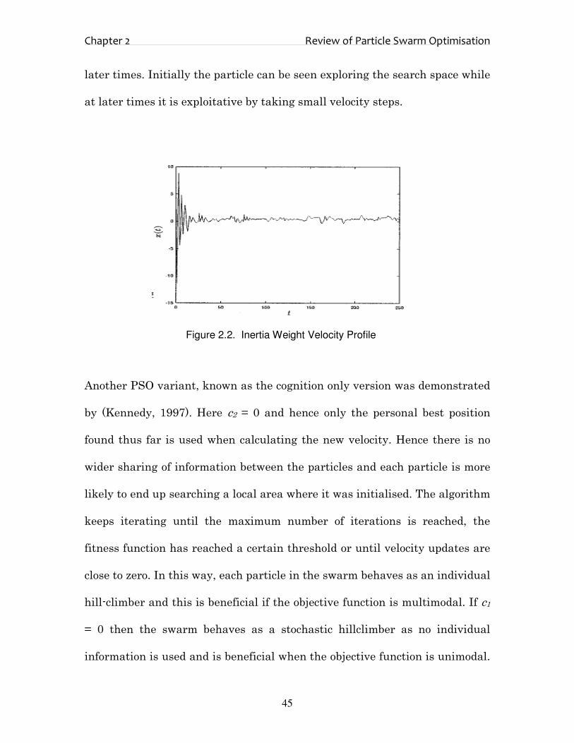
Figure 2.2 displays the typical velocity profile of a particle over each
iteration. The energy dissipating effect of the inertia weight method can
clearly be seen and it is this effect that leads to convergence of the particle at
Pg
Pi
x(t)
w.vij(t) x(t+1)
vij(t)
c2r2(Pg-x(t))
c1r1(Pi-x(t))
Chapter 2 Review of Particle Swarm Optimisation
45
later times. Initially the particle can be seen exploring the search space while
at later times it is exploitative by taking small velocity steps.
Figure 2.2. Inertia Weight Velocity Profile
Another PSO variant, known as the cognition only version was demonstrated
by (Kennedy, 1997). Here c2 = 0 and hence only the personal best position
found thus far is used when calculating the new velocity. Hence there is no
wider sharing of information between the particles and each particle is more
likely to end up searching a local area where it was initialised. The algorithm
keeps iterating until the maximum number of iterations is reached, the
fitness function has reached a certain threshold or until velocity updates are
close to zero. In this way, each particle in the swarm behaves as an individual
hill-climber and this is beneficial if the objective function is multimodal. If c1
= 0 then the swarm behaves as a stochastic hillclimber as no individual
information is used and is beneficial when the objective function is unimodal.

Chapter 2 Review of Particle Swarm Optimisation
46
The coefficients used in (2.2.1) determine the swarm behaviour, and many
studies have been done in order to optimise these coefficients as well as
maintain the explorative ability of the swarm. (Ratnaweera et al, 2004)
proposed time varying acceleration coefficients and the mutation of particles
to address this issue since it has been commonly observed particularly with
benchmark functions, that the PSO finds a good local optima but can remain
stuck in this optima sometimes for the entire duration of the run with little to
no improvement.
A predator-prey type optimiser was introduced in (Silva et al, 2002, Silva et
al, 2003) where a predator particle was used to chase the gbest particle and
the predator randomly repelled particles in the swarm. The extent to which
they were repelled also depended on how close the swarm particle was to the
predator. This method however suffered from determining just how often
swarm particles were to be repelled, and added another level of complexity to
the tuning process. Other methods of gaining better performance include
using mating, breeding and subpopulation mechanisms that were introduced
by (Løvbjerg et al, 2001). Co-operative particle swarm optimisation is another
promising area that has been introduced to allow the swarm to use
information from the genes of different members of the population (van den
Bergh et al, 2000).

Chapter 2 Review of Particle Swarm Optimisation
47
2.4. The Constriction Factor PSO
The canonical PSO can still have fairly large velocities at the end of a run,
hence the reason why inertia weights were introduced in an effort to control
the velocities. The constriction factor PSO is another attempt to control the
particle velocities and was proposed by (Clerc, 1999) as a way of ensuring
convergence. This technique has the following formulation :-
( ) ( ) ( ) ( )])()([1 2211 txPrctxPrctvKtv ijgjijijijij −+−+×=+ (2.4.1)
ϕϕϕ 42
2
2 −−−=K , where ϕ = c1 + c2, applicable for ϕ > 4
In the above formulation, if c1 = c2 = 2.05, K will then be 0.729 and will result in
the previous velocity (momentum term) being multiplied by 0.729 and the (P-
x) being multiplied by 0.729*2.05 = 1.49445 (times a random number between
0 and 1). This is different from the inertia weight formulation where only the
velocity of the previous iteration (momentum term) was lowered at every
iteration, here the entire velocity step is reduced. Intuitively, it is expected
that the velocities in the constriction factor method will decrease much more
rapidly than the inertia weight method, hence leading to convergence.
(Eberhart & Shi, 2000) analysed the constriction factor PSO and concluded
empirically that setting Vmax = Xmax significantly improved their results.

Chapter 2 Review of Particle Swarm Optimisation
48
Furthermore (Zhang, Yu, Hu, 2005) analysed the effect of ϕ on the solution
of unimodal and multimodal problems. ϕ was varied between 4.0 and 4.4.
They concluded that the best choice for unimodal problems was to take ϕ =
4.1 and for multimodal problems ϕ = 4.05.
2.5. Parameter Sensitivities
It is important to have an understanding of the effect of the parameters of
the PSO in order to design a version of the algorithm that would be suitable
for history matching. In order to do this, a test is conducted here on the
canonical, inertia weight and constriction factor versions to gain some insight
to their behaviour. A test function (2.5.1) is used to get an idea of their
velocity profiles.
7.0)2
4cos(4.0)1
3cos(3.022
221
)( +−−+= xxxxxf ππ (2.5.1)
Firstly, the canonical version is tested by varying the acceleration
coefficients. Typically c1 = c2 = 2. Figure 2.3 displays the effect of varying c1 &
c2 from 1.0 to 3.0 on their velocity profiles. There are two aspects that should
be noted from this Figure. Firstly, the velocity magnitudes are proportional to
the acceleration coefficient. Secondly, it doesn’t matter what the coefficient is,
Chapter 2 Review of Particle Swarm Optimisation
49
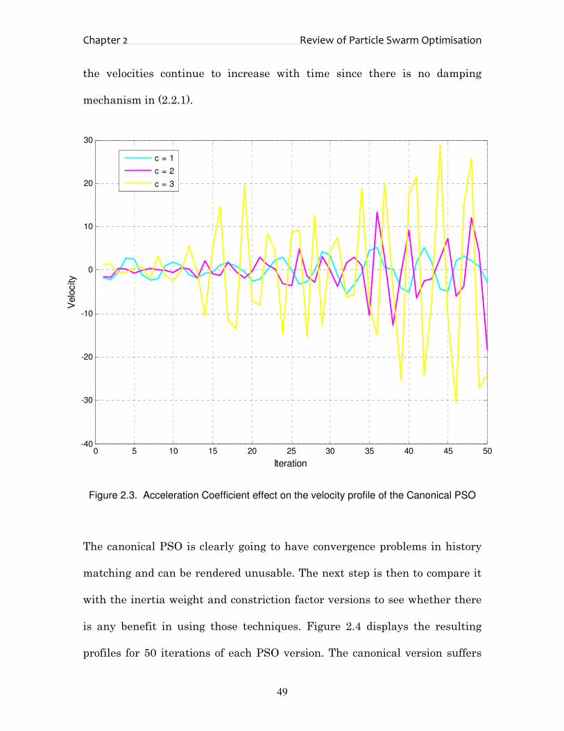
the velocities continue to increase with time since there is no damping
mechanism in (2.2.1).
Figure 2.3. Acceleration Coefficient effect on the velocity profile of the Canonical PSO
The canonical PSO is clearly going to have convergence problems in history
matching and can be rendered unusable. The next step is then to compare it
with the inertia weight and constriction factor versions to see whether there
is any benefit in using those techniques. Figure 2.4 displays the resulting
profiles for 50 iterations of each PSO version. The canonical version suffers
0 5 10 15 20 25 30 35 40 45 50-40
-30
-20
-10
0
10
20
30
Iteration
Velo
city
c = 1
c = 2
c = 3

Chapter 2 Review of Particle Swarm Optimisation
50
from high velocities all through the run and does not converge. The inertia
weight version with w = 0.9 and linearly decreasing to w = 0.4 at the end of
the run also shows fairly high velocities for most of the run, however does
constrain itself towards the end. The constriction factor version quickly
reduces its velocity and is able to make small steps for most of the run, hence
fine tuning its solution.
Figure 2.4. Velocity profile comparison of the Canonical, Inertia Weight and Constriction
Factor PSO’s
0 5 10 15 20 25 30 35 40 45 50-2
-1.5
-1
-0.5
0
0.5
1
1.5
2
Iteration
Velo
city
Canonical PSO
Inertia Weight
Constriction Factor

Chapter 2 Review of Particle Swarm Optimisation
51
The next step is to investigate the effect of changing the inertia weight
ranges to see if any improvement can be made to its convergence behaviour.
A comparison is made with w = 0.9 → 0.4 (Shi et al, 1995), w = 0.4 → 0.9 and
w = 0.5 → 0. Figure 2.5 displays the velocity profiles of this test. Clearly,
varying w = 0.5 → 0 shows convergent behaviour that is even better than the
constriction factor in Figure 2.4.
Figure 2.5. Velocity profile comparison of the Inertia Weight PSO with different w ranges
0 5 10 15 20 25 30 35 40 45 50-2
-1.5
-1
-0.5
0
0.5
1
1.5
2
Iteration
Velo
city
w = 0.9 » 0.4
w = 0.4 » 0.9
w = 0.5 » 0.0

Chapter 2 Review of Particle Swarm Optimisation
52
It does make sense to use this range for the inertia weight as taking it down
to 0 will lead to very small velocities at later iterations and hence be able to
fine tune a search. Although the constriction factor version does have
velocities that are dampened with time, it does not have the flexibility of the
inertia weight as the constriction factor K operates over the entire velocity
update.
The objective is to design a Particle Swarm optimiser suitable for history
matching purposes. The inertia weight version appears to be a better
candidate for further development and it will be used as the basis for the rest
of this thesis.

Chapter 3 Development of a new Particle Swarm Variant
53
Chapter 3
Development of a new Particle Swarm Variant
3.1. The Flexi-PSO
Particle Swarms are similar to fractals. Fractals produced intricate patterns
based on simple recursive equations. Similarly the swarm also produces an
exciting emergence of interaction between its particles that leads to good
solutions in global optimisation also using simple recursive equations. The
analogy of particles interacting at the social level makes intuitive sense and
heuristics can be developed to make the canonical algorithm much more
powerful.
This thesis looks at intuitive mechanisms and heuristics to increase the
effectiveness of the swarm. This will be judged by comparing a particle
swarm variant developed in this thesis viz. the Flexi-PSO (Kathrada, 2009) to
the original Inertia Weight method on a non-convex function. Further tests
will be conducted on benchmark mathematical test sets and the training a
neural network to assess the performance of the Flexi-PSO in relation to
other state of the art techniques.

Chapter 3 Development of a new Particle Swarm Variant
54
The first mechanism that is introduced here is to use an extended particle
swarm optimiser that updates the velocities using pbest, gbest as well as
lbest. lbest here is implemented for a neighbourhood with a ring topology
where each particle has a neighbour on either side of it, with the end member
particles also being connected and hence forming a ring as in Figure 3.1.
Particles are numbered according to the sequence in which they are
initialised.
If the neighbourhood size is taken to be two, then any particle (i) compares
itself to particle (i-1) and particle (i+1), e.g. particle 1 would compare itself to
particle 2 and particle 8 since the topology is a ring. The neighbourhood size
used in this study is 25% of the population size. This idea was also introduced
by (Jun-jie & Zhan-hong, 2005), however it was applied to the constriction
factor method of PSO (Eberhart and Shi, 2000). Here, advantage is taken of
the neighbourhood best position, and this additional information helps the
swarm to search more of the solution space.

Chapter 3 Development of a new Particle Swarm Variant
55
Figure 3.1. Ring Topology for a population of particles
(3.1.1) is the extended PSO equation :-
( ) ( ) ( ) ( ) ( ))()()(1 332211 txPrctxPrctxPrctwvtv ijljijgjijijijij −+−+−+=+ (3.1.1)
r1, r2 and r3 are numbers in the range [0, 1] generated from a uniform random
number generator and are updated for each dimension in each iteration. w is
the inertia weight parameter and is varied linearly down from wmax = 0.5 at
1
5
7
64
3
8 2

Chapter 3 Development of a new Particle Swarm Variant
56
the beginning of the run to wmin = 0.0 at the end of the run. The shorter range
of w used here is to aid exploitation of the particles towards the end of the
run.
The issue then arises as to how to assign the acceleration coefficients. (Jun-jie
& Zhan-hong, 2005) chose various configurations in order to keep the sum of
the acceleration coefficients equal to 4. This is in keeping with the original
PSO where c1 = 2 and c2 = 2. In this study a dynamic approach has been used
to select the acceleration coefficients for each particle and on every iteration.
The simple heuristic that is followed is that a flexible PSO is desired to be
able to deal with both multimodal and unimodal problems. The acceleration
coefficient heuristic for d variables is represented as follows :-
for i = 1:d (3.1.2)
if rand() < 0.333
then c1i = 2.0, c2i = 0.0, c3i = 0.0
elseif rand() > 0.666
then c1i = 0.0, c2i = 2.0, c3i = 0.0
else
c1i = 1.333, c2i = 1.333, c3i = 1.333
end

Chapter 3 Development of a new Particle Swarm Variant
57
where rand() is a uniformly drawn random number in the range [0,1]. Hence
each particle on each iteration has an equal probability of either acting as an
individual hillclimber, a stochastic hillclimber or to use both cognitive and
social information from the swarm. This makes the swarm as a whole much
more flexible in being able to deal with an objective function, particularly if
one does not have much idea of what the fitness landscape may look like.
The underlying motto behind this enhancement is “Big moves coupled with
small moves”. In the traditional inertia weight formulation, particles in the
swarm are more likely to make big moves in the search space which
progressively decreases with each iteration. Conceptually this leads to a big
problem, in that a particle may be in a valley which contains the global
minimum of the function, but because the particles are taking large steps,
they can easily fly out of this region to a poorer region. However, if the swarm
can be designed such that from outset, it does have the possibility of making
small moves as well as big moves, this can greatly enhance its convergence
and explorative ability.
There have been other techniques that have explored the same idea but with
a different implementation. (Li et al, 2007) proposed a random velocity
boundary condition on the swarm such that at each iteration, Vmax was set

Chapter 3 Development of a new Particle Swarm Variant
58
randomly so that particles now had a higher probability of taking small
moves early on in the run.
The next issue that arises in the implementation is how to deal with particles
that go out of the boundary range. Figure 3.2 depicts different mechanisms
that can be employed.
Figure 3.2. Boundary handling mechanisms
In Figure 3.2a, the boundary acts as an absorbing wall, effectively stopping
the particle from going any further. This can be especially useful for those
functions whose optimum is located at the boundary. In Figure 3.2b, the
particle is reflected back into the search space by reversing its velocity after

Chapter 3 Development of a new Particle Swarm Variant
59
impact with the boundary wall. In Figure 3.2c the particle is allowed to
escape the boundary but this particle is typically ignored when it comes to
being function evaluated. Finally in Figure 3.2d the velocity is reversed and
dampened when it impacts the boundary wall.
The damping wall boundary handling mechanism is chosen to be used in the
Flexi-PSO. The absorbing walls mechanism does appear attractive at first
glance particularly since functions can have their optimums on the boundary,
however in practise it was found to lead to many redundant function
evaluations. The problem arises that once the particle is stopped at the
boundary, for it to get back into the search space can take many iterations
since the sign of the velocity needs to be reversed. Reflecting walls were
deemed to be inappropriate since the particle is reflected right back and this
can equally lead to many redundant function evaluations if the optimum is
near the boundaries. Invisible walls were not considered since a history
match function evaluation is desired for every iteration and it would be a
waste of the distributed computing resources to subtract a function
evaluation on an iteration. Damping walls is the most attractive option since
function evaluations are not wasted, and at the same time the particle can
move progressively closer to the boundary if indeed the optimum is located
close to it.

Chapter 3 Development of a new Particle Swarm Variant
60
3-Dimensional animations over a benchmark function presented later in this
paper are used to give a qualitative understanding of the behaviour of the
swarm. It was found that while the acceleration coefficient heuristic did allow
particles some degree of freedom, at the end of the run they still tended to
congregate very closely around the gbest and lacked the desired explorative
ability. This was wasteful as often the particles congregated around the gbest
early on in the run with the result that the particles had very small velocities
and from that point onward were only performing local exploitation with
little improvement in the gbest. This is an intrinsic drawback of the particle
swarm method as the entire swarm surrounds an attractor and cannot break
free from it to search a wider area. If w were varied from wmax = 0.9 to wmin =
0.4 then the particles tend to flicker around the gbest with little ability to fine
tune the search as also noted by (Vesterstroem et al, 2002).
This premature convergence problem was addressed using the following
heuristics. One half of the population should be allowed to perform local
exploitation (denoted as “exploitation” particles) while the other half (denoted
as “exploration” particles) should be repelled from gbest if they came too close
to it. As a measure of “closeness” to the gbest, the repulsion is induced in two
ways. If an exploration particle comes to within a fitness tolerance or a
distance tolerance of the gbest, then a perturbation to a randomly selected
dimension of the velocity vector is added. The fitness repulsion is invoked

Chapter 3 Development of a new Particle Swarm Variant
61
when the difference between fitness of the exploratory and gbest particles is
less than a fitness tolerance ε viz.
ε≤− gbesti ff (3.1.3)
The distance repulsion is invoked when the normalised absolute difference
between the exploratory and gbest particles in all dimensions is less than a
threshold of the search range viz.
α≤−
−
min,max,
,
jj
jgj
XX
PX, j ∈ [1,d] (3.1.4)
Once a repulsion is invoked for an exploration particle, the velocity is
perturbed in a randomly selected dimension and is represented in equation
(3.1.5):
( )2
1 max
4
Vrtvij =+ (3.1.5)
where r4 is a random number drawn uniformly in the range [-1,1].
Qualitative animations using this concept of exploration and exploitation
particles showed “atomic-like” behaviour, similar to what was observed by
(Blackwell and Branke, 2004). This “atomic-like” behaviour is explained by

Chapter 3 Development of a new Particle Swarm Variant
62
the observation that whenever an exploration particle came too close to the
gbest it was repelled outwards only for it to be attracted back to the gbest
where it was once again repelled outwards. However this repulsion often
enables particles to find better solutions. The repulsion step size is set
proportional to half of Vmax. If there is some idea as to how far apart the
optima are expected to be on the fitness landscape then this step size can be
set accordingly. The exploitation particles on the other hand close in on the
gbest and try to improve it by doing a fine local search. If an exploration
particle finds a better gbest, then the rest of the swarm moves towards this
new position and the process continues until the termination criterion is met.
Figure 3.3 displays the pseudo-code for the entire procedure.

Chapter 3 Development of a new Particle Swarm Variant
63
Begin
initialize the population
initialize the velocities
evaluate fitness of all particles
set current position as pbest, set particle with best fitness as gbest and find
the neighbourhood lbests
While iter < total_iterations
update inertia weight factor (2.3.4)
set acceleration constants with (2.4.2)
For i = 1 to population
update fitness distance (fd) and variable difference (vd) using
(2.4.3) and (2.4.4) respectively
If fd > ε | fd = 0 | vd > α | 2
populationi ≤
For j = 1 to dimensions
update velocities (2.4.1)
check velocity magnitudes with (2.3.2)
EndFor j
Else
reset acceleration constants
pick = rand().dimensions // is the ceiling operator
For j = 1:dimensions
If j ≠ pick
update velocities with (2.4.1)

Chapter 3 Development of a new Particle Swarm Variant
64
Else
update velocities with (2.4.5)
check velocity magnitudes with (2.3.2)
EndIf
EndFor j
EndIf
EndFor i
update positions with (2.3.3)
evaluate fitness of all particles
update pbest, gbest and lbest if necessary
EndWhile
End
Figure 3.3. Pseudo-code for the Flexi-PSO
3.2. Qualitative Behaviour of the PSO
In order to gain a greater understanding of the behaviour of the swarm, some
qualitative analysis from experiments is necessary. To this end 3-dimensional
animations have been set up for the following function (3.2.1) {same as (2.5.1)
presented earlier & will red thread its way through this thesis} :-
7.0)2
4cos(4.0)1
3cos(3.022
221
)( +−−+= xxxxxf ππ (3.2.1)

Chapter 3 Development of a new Particle Swarm Variant
65
This is a highly multimodal function with many local minima and is depicted
in Figure 3.4.
Figure 3.4. 3-D plot of multimodal Equation (3.2.1)
-2-1
01
2
-2-1
01
20
2
4
6
8
10
12
x1x2
f(x)
Chapter 3 Development of a new Particle Swarm Variant
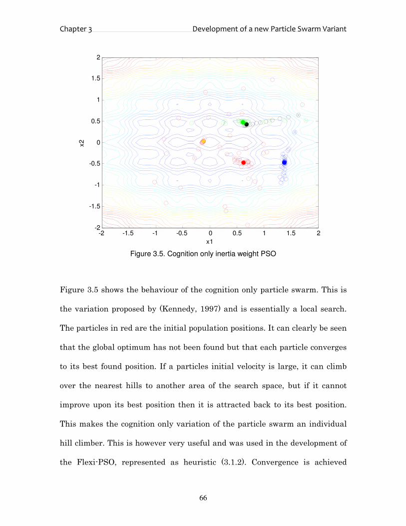
66
Figure 3.5. Cognition only inertia weight PSO
Figure 3.5 shows the behaviour of the cognition only particle swarm. This is
the variation proposed by (Kennedy, 1997) and is essentially a local search.
The particles in red are the initial population positions. It can clearly be seen
that the global optimum has not been found but that each particle converges
to its best found position. If a particles initial velocity is large, it can climb
over the nearest hills to another area of the search space, but if it cannot
improve upon its best position then it is attracted back to its best position.
This makes the cognition only variation of the particle swarm an individual
hill climber. This is however very useful and was used in the development of
the Flexi-PSO, represented as heuristic (3.1.2). Convergence is achieved
x1
x2
-2 -1.5 -1 -0.5 0 0.5 1 1.5 2-2
-1.5
-1
-0.5
0
0.5
1
1.5
2

Chapter 3 Development of a new Particle Swarm Variant
67
much quicker by allowing each particle to randomly use the cognition only
variation.
Figure 3.6 and Figure 3.7 are contour plots of this function upon which the
history of a swarm run using the Inertia Weight PSO and Flexi-PSO are
superimposed respectively. Each run comprised of 10 particles and 100
iterations. The red circles in both figures are the initial population positions.
In Figure 3.6 the population is deliberately initialised away from the global
optimum and in a small volume of the search space yet the swarm is still able
to migrate its way to the global optimum. The efficiency of the Flexi-PSO
algorithm (Figure 3.7) is clear as there is a dense cluster of particles
searching the niche with the global optimum and a sparse search away from
this niche. Other nearby niches have also been searched. This is especially
important in history matching due to the expensive computational time for
each function evaluation and it is along these lines that further development
of the algorithm has been carried out. In contrast the traditional inertia
weight PSO (Figure 3.6) converges much slower to the global optimum.
In Figure 3.7 the Flexi-PSO exhibits repulsion along the principal axis as
equation (3.1.5) is invoked for a single dimension only. For rotated functions,
the repulsion can be invoked in multiple dimensions.
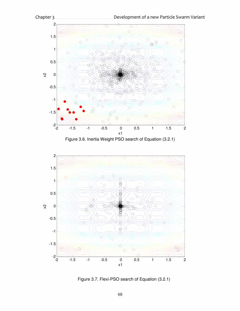
Chapter 3 Development of a new Particle Swarm Variant
68
Figure 3.6. Inertia Weight PSO search of Equation (3.2.1)
Figure 3.7. Flexi-PSO search of Equation (3.2.1)
x1
x2
-2 -1.5 -1 -0.5 0 0.5 1 1.5 2-2
-1.5
-1
-0.5
0
0.5
1
1.5
2
x1
x2
-2 -1.5 -1 -0.5 0 0.5 1 1.5 2-2
-1.5
-1
-0.5
0
0.5
1
1.5
2

Chapter 3 Development of a new Particle Swarm Variant
69
(Vesterstroem et al, 2002) proposed a diversity metric in order to measure the
convergence behaviour of the swarm. This metric is simply a summed
average distance measure of each particle from the mean position of the
swarm given in (3.2.2) where n is the number of particles and d the number
of dimensions :-
( )∑ ∑= =
−=n
i
d
j
jij xxn
diversity1 1
21 (3.2.2)
This metric is independent of the shape of the objective function, and is a
qualitative indicator of the behaviour of the swarm. Figure 3.8 is an
illustration of the diversity of the traditional inertia weight PSO versus the
Flexi-PSO.

Chapter 3 Development of a new Particle Swarm Variant
70
Figure 3.8. Diversity metric of the swarm history
It can be immediately seen that the Flexi-PSO converges quicker than the
traditional inertia weight formulation but that it also maintains a level of
diversity at later iterations by repulsion of the exploration particles thus
enabling the Flexi-PSO to escape local minima more easily. These are key
elements for history matching as we do want to get to a match as quick as
possible but be flexible enough to move on searching for other suitable
matches as well. This is further illustrated in the velocity profiles of both
methods in Figure 3.9 of variable x1.
0 10 20 30 40 50 60 70 80 90 1000
0.2
0.4
0.6
0.8
1
1.2
1.4
1.6
iteration #
div
ers
ity
Flexi-PSO
Inertia Weight PSO

Chapter 3 Development of a new Particle Swarm Variant
71
Figure 3.9. Velocity profile of variable x1
Figure 3.10. Global best value history
0 10 20 30 40 50 60 70 80 90 10010
-20
10-15
10-10
10-5
100
105
iteration #
glo
balb
est
Flexi-PSO
Inertia Weight PSO
0 10 20 30 40 50 60 70 80 90 100-2
-1.5
-1
-0.5
0
0.5
1
1.5
2
iteration
velo
city (
x1)
Flexi-PSO
Inertia Weight PSO

Chapter 3 Development of a new Particle Swarm Variant
72
Figure 3.10 also shows that Flexi-PSO reaches the true global optimum
faster than the inertia weight method, once again due to the modifications
made to it. The Flexi-PSO appears to halt at around iteration 75 however this
is just due to the precision of MATLAB being reached.
3.3. Sequential Niching
The Flexi-PSO does have the ability to escape local minima more easily than
traditional PSO formulations, however the goal of this thesis is to develop an
algorithm for history matching that would be able to find multiple niches to
be used in uncertainty modelling. To this end niching variations of the PSO
have been investigated.
Two variations of niching algorithms exist viz. parallel and sequential
niching. Parallel niching seeks to locate and maintain several niches in a
population simultaneously and the fitness landscape is not modified in doing
so. The challenge is in finding a good measure to locate possible solutions and
to organise individuals in the population around solutions. Sequential
niching methods on the other hand successively locate and isolate niches such
that future searches do not duplicate sampling in niches that have already
been identified, usually by modifying the fitness landscape around the niche.

Chapter 3 Development of a new Particle Swarm Variant
73
There have been many studies on niching using genetic algorithms but very
little using particle swarms. Fitness sharing and deterministic crowding are
popular techniques employed in genetic algorithms for locating multiple
optima. A seminal paper on sequential niching using fitness sharing GA’s is
by (Beasley et al, 1993). In this paper, fitness sharing was used to locate
niches, and derating functions applied to modify the fitness function within
the niche radius. Fitness sharing was introduced by (Goldberg, 1987) and is a
technique that modifies the fitness landscape by lowering an individual’s
fitness by an amount nearly equal to the number of individuals within the
same niche.
The primary drawback to this approach is that the niche radius calculation
requires prior knowledge of the number of optima in the fitness function. This
is something that clearly cannot be used in history matching or when
working with “black boxes” as the number of optima are unknown.
Nevertheless this paper did highlight key elements in sequential niching viz.
selection of an appropriate derating function such that false optima are not
created (mexican hat effect) and estimation of the niche radius. Deterministic
crowding is another method introduced by (Mahfoud, 1995) that uses
competition between parents and children in the same niche. Essentially

Chapter 3 Development of a new Particle Swarm Variant
74
after crossover and mutation, each child replaces its nearest parent if it has a
better fitness.
There have been a few attempts at using particle swarms to find multiple
niches. (Engelbrecht, 2005) argued that the gbest PSO was incapable of
niching while the lbest PSO was inefficient. Nevertheless there have been
studies on modifying the basic algorithm that have achieved some success.
(Kennedy, 2000) used a clustering technique that assigns each particle to a
cluster and substitutes the cluster centre for the particle’s personal best.
Although a niche radius is not employed in this approach, it is necessary to
set the number of clusters before hand, which can be difficult to estimate for
different functions particularly “black boxes”. (Brits et al, 2002) proposed a
cognition only model that iterates and when there is little improvement, a
sub-swarm is created around the particle in a small area to further refine the
search. The algorithm is however dependent on proper initial distribution of
the particles, something which cannot be guaranteed for complex functions.
(Zhang et al, 2005) attempted using the concepts in fitness sharing GA’s to
train multiple sub-swarms by employing a power law derating function and
calculating the niche radius from a prior knowledge of the fitness landscape.
They do however introduce an interesting concept of convergence similar to

Chapter 3 Development of a new Particle Swarm Variant
75
the diversity metric used by (Vesterstroem et al, 2002) to stop the training of
each sub-swarm.
(Vaz & Fernandes, 2005) used the inertia weight PSO in conjunction with an
approximate descent direction to enable the computation of multiple niches.
This is an interesting approach though somewhat computationally expensive
since gradients need to be calculated for each particle at each iteration, and
would not be appropriate for functions with discrete variables.
(Zhang et al, 2006) proposed one of the most rigorous methods of sequential
niching in particle swarms with the only drawback being the computational
expense of additional function evaluations to estimate the niche radius. They
successively train sub-swarms to find new niches by isolating old niches
using the hill valley function approach which continuously moves in each
dimension taking interior sample points until the monotonic change in the
fitness stops. This is very well suited to mathematical functions but not
expensive function evaluations.
Since run times in reservoir simulation models can be quite long, and the
simulator is a “black box” many of these approaches would not be suitable. In
niching the primary elements are choice of a suitable derating function to
steer the algorithm away from previously identifies niches and estimation of

Chapter 3 Development of a new Particle Swarm Variant
76
the niche radius. The approach taken in this thesis is not to use a derating
function due to the computational expense. Instead any particle falling
within a previously identified niche is not evaluated but accelerated out of
that niche instead. It is difficult to address the second problem of choosing a
niche radius as each simulation model is going to have a completely different
fitness landscape and hence we are left with either trying to rigorously
evaluate the niche radius by making many more function evaluations or
empirically set the niche radius beforehand and live with a certain amount of
inefficiency.
In this study, neural networks were used to train the sampled points once
there was less than a 2% improvement in the globalbest over the last 5
iterations. Once the neural network was trained, it was then interrogated in
both directions of each dimension to estimate the niche radius, however this
was found to be ineffective due to the scarcity of sample points. This becomes
a contradictory problem since niches need to be identified with the fewest of
function evaluations whereas neural networks being proxy models require
large amounts of data to be trained with to be effective and this line of work
was abandoned.
The niche radius is now taken as a user defined limit and in this study is set
to 10% of the dimensional range of each variable. This radius is purely up to

Chapter 3 Development of a new Particle Swarm Variant
77
the user to define as the niche radius will vary within each function, vary
with different objective functions and for different problem setups, hence
there is no further sensitivity study on this parameter in this thesis. Figure
3.11 shows the effect of adding this to the Flexi-PSO.
The lowest valleys are extensively sampled by the swarm using the same
number of function evaluations as in the previous cases. Once there is no user
specified threshold improvement within a user specified number of iterations,
the global best position is cordoned off by the niche radius and the swarm is
reinitialised randomly ensuring that no particle is reinitialised in the
cordoned off area. To preserve useful information that the swarm already
has, the global best on re-initialisation is set to the best position visited by
the swarm that is not in the niche cordoned area. Figure 3.12 shows the
pseudo-code for this procedure.

Chapter 3 Development of a new Particle Swarm Variant
78
Figure 3.11. Sequential Niching Flexi-PSO search of Equation (3.2.1)
Figure 3.12 displays the pseudo-code for the Sequential Niching Flexi-PSO.
x1
x2
-2 -1.5 -1 -0.5 0 0.5 1 1.5 2-2
-1.5
-1
-0.5
0
0.5
1
1.5
2

Chapter 3 Development of a new Particle Swarm Variant
79
Begin
initialize the population
initialize the velocities
evaluate fitness of all particles
set current position as pbest, set particle with best fitness as gbest and find
the neighbourhood lbests
While iter < total_iterations
update inertia weight factor (2.3.4)
set acceleration constants with (2.4.2)
For i = 1 to population
update fitness distance (fd) and variable difference (vd) using
(2.4.3) and (2.4.4) respectively
If fd > ε | fd = 0 | vd > α | 2
populationi ≤
For j = 1 to dimensions
update velocities (2.4.1)
check velocity magnitudes with (2.3.2)
EndFor j
Else
reset acceleration constants
pick = rand().dimensions // is the ceiling operator
For j = 1:dimensions
If j ≠ pick
update velocities with (2.4.1)

Chapter 3 Development of a new Particle Swarm Variant
80
Else
update velocities with (2.4.5)
check velocity magnitudes with (2.3.2)
EndIf
EndFor j
EndIf
EndFor i
update positions with (2.3.3)
For I = 1 to population
While (niches > 0 & particle lies within any niche)
Reinitialise particle randomly
EndWhile
EndFor
evaluate fitness of all particles
update pbest, gbest and lbest if necessary
if |gbest(iter) – gbest(iter-user_iter)| < tolerance
set niche boundary = gbest ± niche_radius
reinitialise population
reinitialise velocities
set gbest = best position found outside niche boundary
EndWhile
End
Figure 3.12. Pseudo-code for the Sequential Niching Flexi-PSO

Chapter 3 Development of a new Particle Swarm Variant
81
3.4. Function Stretching
Function Stretching is a technique that can be used to find multiple minima.
(Parsopoulos et al, 2004) proposed a two-phase transformation of the
objective function once a detected minimum has been found. The first phase
stretches the objective function upwards eliminating all minima with values
higher than the detected minimum. In the next stage, the detected minimum
is turned into a maximum whilst still leaving all minima with objective
function values lower than the detected minimum unaltered.
Let x* be a minimiser of an objective function f. The stretching is defined as :-
( ) ( ) ( ) ( )( )( )1**1 +−−+= xfxfsignxxxfxG γ (3.4.1)
( ) ( ) ( ) ( )( )( ) ( )( )( )*tanh
1*2
xGxG
xfxfsignxGxH
−
+−+=
µγ (3.4.2)
where γ1 = 5000, γ2 = 0.5 and µ = 10e-10 are arbitrary parameters. The
following function is used to evaluate whether this transformation process
can be useful in the history matching process.
( ) ( ) 10cos.sin ++= xxxy (3.4.3)

Chapter 3 Development of a new Particle Swarm Variant
82
Figure 3.13. Plot of (3.4.3)
Figure 3.13 illustrates (3.4.3). This function is then taken through the two-
stage transformation process and is depicted in Figure 3.14. The local
minimum used is x* = 3.68 (highlighted in Figure 3.12). G stretches the
function upwards and H has turned this local minimum into a maximum
whilst leaving everything lower than f(x*) = 6.328 intact. This appears to be a
promising technique that can be used in conjunction with the PSO however, if
the first detected minimum is indeed the global minimum, then no other
minima will be detectable thereafter and the algorithm will have to be rerun,
albeit you are better off since the global minimum is now known.
0
2
4
6
8
10
12
14
16
18
20
-10 -8 -6 -4 -2 0 2 4 6 8 10
X
Y

Chapter 3 Development of a new Particle Swarm Variant
83
Figure 3.14. Function Stretched depiction of minimum @ x* = 3.68
Figure 3.15 shows the effect of the stretching transformation on the global
minimum at x* = 9.61. In a way, one would actually hope that the first
minimum that is found is not the global minimum with this technique, but it
does lend itself to the Flexi-PSO since the Flexi-PSO has the ability to take
small steps and hence find a local minimum quicker than its counterparts.
Testing this technique on a local minimum ( x* = [-0.6 –0.5], f(x)* = 0.9127 )
gives the transformed fitness landscape in Figure 3.16. Figure 3.17 then
shows the globalbest progression when the Flexi-PSO is run on this
transformed function.
0.1
1
10
100
1000
10000
100000
1000000
10000000
100000000
1000000000
-10 -8 -6 -4 -2 0 2 4 6 8 10
X
Yf G H

Chapter 3 Development of a new Particle Swarm Variant
84
Figure 3.15. Function Stretched depiction of global minimum @ x* = 9.61
The Flexi-PSO is not initialised anywhere in the area of the hollows of Figure
3.15, since the initial globalbest value is in the region of 105, and the Flexi-
PSO is still able to make its way into the hollows of the transformation and
find the global optimum. This technique looks promising and will be
attempted when history matching the case studies presented later in this
thesis.
0.1
1
10
100
1000
10000
100000
1000000
10000000
100000000
1000000000
-10 -8 -6 -4 -2 0 2 4 6 8 10
X
Yf G H

Chapter 3 Development of a new Particle Swarm Variant
85
Figure 3.16. Function Stretched depiction of local minimum @ x* = [-0.6 –0.5] on (3.2.1)
Figure 3.17. Flexi-PSO performance on the function stretched transformation of (3.2.1)
-2-1.5
-1-0.5
00.5
11.5
2
-2
-1.5
-1
-0.5
0
0.5
1
1.5
2
0
0.5
1
1.5
2
2.5
x 105
x1
x2
f(x)
0 10 20 30 40 50 60 70 8010
-20
10-15
10-10
10-5
100
105
1010
Iterations
fitn
ess

Chapter 3 Development of a new Particle Swarm Variant
86
3.5. Handling Mixed Integer Problems
Another area of particular importance in history matching is mixed integers.
Mixed integer problems are where you have both discrete variables and
continuous variables simultaneously in the problem formalisation. This is
relevant to history matching as the most common approach has been to use a
single static model and deterministically find a suitable history match, but
this approach was largely due to a lack of computing power. With widely
available distributed computing resources and reservoir simulators that can
decompose the grid and run the sub-grids in parallel over multiple
processors, past limitations are no longer that critical. This opens the way for
wider uncertainty handling by using multiple static models either based on
different grids, geological models or property realisations. Hence when the
assisted history match is launched, the Flexi-PSO will sample from the
available static models (discrete variable/s) and fluid/rock parameters
(continuous variables) simultaneously and gravitate towards the static
model/s that give the best performance on the objective function.
This turns the history match problem from being solely in the continuous
domain to the mixed integer domain. In our case it is unlikely that binary
integer problems arise, but it is more of a case where an integer variable can
take on a number of discrete values e.g. realisation 1, realisation 2 etc. There

Chapter 3 Development of a new Particle Swarm Variant
87
have been quite a few attempts at mixed integer problems using particle
swarms of which a few will be mentioned. (Gaing, 2005) used a simple
rounding off method in the velocity updates for the discrete variables. Hence
(3.1.1) would be rounded off to give a discrete value that would then be used
in the position update. (Rongshan & Xia, 2007) proposed using the sigmoid
function (commonly used as transfer functions in neural networks) to deal
with binary integer problems. The updated velocity is used as the sigmoid
function argument and the position is updated as zero if the sigmoid function
result is less than a uniform random value within [0,1] and 1 otherwise.
(Kitayama & Masuda, 2006) developed a penalty function approach to
handling discrete variables. In the velocity updates all variables are treated
as continuous but the fitness function is augmented with a penalty if the
continuous equivalent of the discrete variables departs from discrete values.
In this study a simple round-down approach to each discrete variable is
taken, where the discrete variable represented in the swarm is just the index
to the actual underlying variable value. This is by far the simplest approach
to mixed integer problems and is used in a mathematical benchmark function
test in the next chapter to test its effectiveness. (3.5.1) formalises this
representation for tubing sizes :-

Chapter 3 Development of a new Particle Swarm Variant
88
Actual size (ID) : [ 1.867”, 2.259”, 2.323”, 2.441”, 3.068” ]
PSO index : X = [1, 2, 3, 4, 5]
PSO update (2.3.3) : x = 1.45 → X = floor(x) = 1 (3.5.1)
Function evaluation : f(X) = f(1.867”)

Chapter 4 Mathematical Testing of the Flexi-PSO
89
Chapter 4
Mathematical Testing of the Flexi-PSO
4.1. CEC 2005 benchmark test set
There have been many optimisation methods proposed over the years for
history matching but there has been no qualitative way of judging their
effectiveness in relation to other each other, except for those that have used a
common benchmark test model like the Imperial College Fault model. In this
study 25 non-linear functions have been used as an experiment to gauge how
well the Flexi-PSO can deal with unimodal and highly multimodal functions.
The test set is developed by (Suganthan et al., 2005) for the 2005 Congress on
Evolutionary Computation Special Session on Real Parameter Optimisation.
This test set in particular is good to assess bias in algorithms as many
functions are shifted and rotated. Details of these functions can be found in
Appendix A.
Some functions are asymmetrically initialised to assess the robustness of the
algorithm. When the PSO was first introduced, symmetric initialisation was
common where the initial population was uniformly distributed in the entire
search space. (Angeline, 1998) suggested initialising the population

Chapter 4 Mathematical Testing of the Flexi-PSO
90
asymmetrically, where the population is initialised in only a portion of the
search space and away from the global optimum.
Each function was run twenty five times so as to obtain a mean fitness value
and standard deviation, and each run used a different seed for the random
number generator hence each population initialisation was different. All the
runs were conducted in 10 dimensions, using a population size of 20 particles
for 500 iterations resulting in 10 000 function evaluations per trial. A
comparison is made with another PSO paper presented by (Liang &
Suganthan, 2005) in which a dynamic multi-swarm inertia weight method is
combined with a quasi-Newton search method to improve local optimisation.
In order to maintain parity, the Flexi-PSO is combined with the quasi-
Newton (Fletcher, 1970) option FMINUNC within MATLAB. The Flexi-PSO
uses the first 9500 function evaluations whilst the last 500 function
evaluations use the FMINUNC function. Figure 4.1 and Table 4.1 displays
the comparison of the mean values achieved between these two methods in
addition to a differential evolution (Tasgetiren et al, 2005) and memetic
algorithm (Molina et al, 2005) presented at the conference. (Tasgetiren et al,
2005) present results for only the first 14 functions.
The first five functions are unimodal functions; function 1 is the Shifted
Sphere Function, function 2 the Shifted Schwefel’s problem 1.2, and function

Chapter 4 Mathematical Testing of the Flexi-PSO
91
3 the Shifted Rotated High Conditioned Elliptic function. These three
functions have different condition numbers leaving them in increasing order
of difficulty respectively. The condition number associated with a problem is
a measure of that problem's amenability to digital computation, that is, how
numerically well-conditioned the problem is. A better result is achieved for
function 1 than function 2 which in turn is better than function 3. Function 4
is shifted Schwefel’s problem 1.2 with noise in fitness which makes the
search process much more difficult. The Flexi-PSO does show good
performance on this function relative to the other techniques but is still far
from the optimum.
Function 5 is Schwefel’s problem 2.6 with the global optimum on the bounds.
For 10-D, 3 dimensions are on the low bounds, 3 dimensions on the high
bounds and other 4 dimensions randomly distributed in the search range.
The Flexi-PSO does not perform very well on this problem mainly due to the
fact when a particle goes out of the search space it is damped back in the
search space rather than limiting the position to the boundary. In practice
this can be problematic with particle swarms as it can take many iterations
for the particle to move back into the search space if it is stopped at the
boundary and many function evaluations are wasted during this time.

Chapter 4 Mathematical Testing of the Flexi-PSO
92
Functions 6-25 are multimodal problems. Function 6 is the Shifted
Rosenbrock’s Function, a problem between unimodal and multimodal and an
algorithm with good local search ability can achieve good results on
Rosenbrock’s Function. The Flexi-PSO achieves a good comparable
performance. Function 7 is the Shifted Rotated Griewank function without
bounds, only the initialization range is given and the search range is [−∞,+∞].
Griewank’s function is more difficult with decreasing dimension and it is
difficult to achieve the global optimum. The Flexi-PSO performs relatively
well on this function. Function 8 is the Shifted Rotated Ackley function with
global optimum on bounds, which has a very narrow global basin and half the
dimensions of this basin are on the bounds. This is akin to finding a needle in
a haystack and the Flexi-PSO is not able to find the minimum on any run.
Functions 9 and 10 are shifted Rastrigin’s function and shifted rotated
Rastrigin’s function respectively, both of which have a huge number of local
optima. The Flexi-PSO performs well on all 25 runs for function 9, but the
results are poorer for function 10 owing to the rotation. Function 11 is the
Shifted Rotated Weierstrass function and the poor results that the Flexi-PSO
achieves is due to the complexity of this function. Function 12 is Schwefel’s
problem and for the 100 000 feval case, the optimum is found more than half
the time but when it fails to locate the optimum region, it results in a
solution with a poor fitness. Functions 13 and 14 are expanded functions on

Chapter 4 Mathematical Testing of the Flexi-PSO
93
which the Flexi-PSO performs relatively well, while functions 15-25 are
eleven novel composition functions. They are composed of basic functions and
are extremely challenging to any search algorithm. The Flexi-PSO performs
poorly on all these functions but as can be seen from Figure 4.1 and Table
4.1, to be relatively the same as the other algorithms.
The Flexi-PSO compares well with other methodologies and gives confidence
for further use. Figure 4.2 and Table 4.2 compare the performance on the
same function set but this time in 30 dimensions and for 100 000 function
evaluations. The population size is increased to 40 particles for this test and
the results are once again averaged over twenty five runs. The Flexi-PSO is
compared to a Flexible Evolutionary Algorithm (Alonso et al, 2005), Real
Coded Memetic Algorithm (Molina et al, 2005) and a steady state Real
Parameter Genetic Algorithm (Ballester et al, 2005).
It is evident from Table 4.2 that the Flexi-PSO outperforms the other
techniques on most of the functions underlining its scalability to higher
dimensions. One reason for this is that the Flexi-PSO maintains explorative
capability through the exploration particles even when the exploitative
particles begin to converge, hence the swarm as a whole can continually
search the dynamic range.

Chapter 4 Mathematical Testing of the Flexi-PSO
94
Figure 4.1. CEC-2005 Comparison (10-D, 100 000 fevals)

Chapter 4 Mathematical Testing of the Flexi-PSO
95
Function Random Search
DE RCMA DMS-PSO Flexi-PSO
1 3972.6 18.816 0.00000459 0.0048732 6.0999E-09
2 9856 194.33 3.659 100.7 0.0001715
3 6.32E+07 1001049 515354.8 843760 343160
4 7777.8 267.16 553.511 270.52 5.5735
5 11920 0.0188126 125.378 52.905 516.32
6 3.83E+08 15560 7.10789 82.235 27.273
7 2271.6 1.3767 0.484082 0.84928 0.33796
8 20.509 20.547 20.247 20.365 20.415
9 74.54 35.894 5.309446 7.4393 0.75681
10 90.36 50.082 8.832397 23.521 19.82
11 10.798 9.78996 7.334553 7.3131 4.9684
12 54498 2912.3144 264.37 1180.7 3813.8
13 6.6614 4.99484 1.425342 1.3832 0.70825
14 4.1269 3.99999936 3.513988 3.3758 3.4664
15 727.08 305.706 131.28 296.6
16 340.69 112.8299 141.05 142.41
17 414.52 156.661 161.23 155.1
18 1178.6 806.7819 897.28 922.45
19 1118.3 772.03 879.85 863.56
20 1079.9 800.116 901.32 935.48
21 1352.4 741.413 851.41 1023.9
22 1045.2 721.052 756.64 854.66
23 1377.8 981.28 860.76 1127.8
24 1312.2 224.017 248.75 421.75
25 1338.4 399.9965 1005.7 499.89
Table 4.1. Comparison between Random Search, Differential Evolution, Real-Coded
Memetic, Dynamic Multi-Swarm and Flexi-Particle Swarm Optimisation Algorithms on
the CEC 2005 Mathematical Benchmark Test Set (best solution in bold) for 10-D, 10 000
fevals

Chapter 4 Mathematical Testing of the Flexi-PSO
96
Figure 4.2. CEC-2005 Comparison (30-D, 100 000 fevals)

Chapter 4 Mathematical Testing of the Flexi-PSO
97
Function Random Search
FEA RCMA SPC-PNX Flexi-PSO
1 61517 117.33 9.53E-09 9.3524E-09 1.6389E-11
2 74634 3573.8 7.289625 5.8753 1.9705E-07
3 5.47E+08 17094000 5508628 3317500 40481
4 77629 14525 779.1663 6.8783 5614.6
5 31898 10174 2213.529 4336.6 6035.8
6 1.96E+10 514.15 61.4232 868.07 3.2214
7 9833.6 11.137 0.01329727 0.95537 0.020672
8 20.975 20.464 20.79068 21 20
9 415.46 42.879 7.550987 143.38 2.6034E-12
10 638.52 217.37 110.197 170.61 103.63
11 40.951 31.486 34.65414 18.119 26.395
12 1.13E+06 31652 6432.686 23408 1193.8
13 181.72 7.3701 8.659078 3.7176 1.6729
14 13.784 13.057 12.747 13.452 12.521
15 926.61 331 356.1009 368.29 354.35
16 701.59 269.95 335.0033 133.34 250.61
17 776.21 338.36 296.6728 124.14 270.19
18 1236.1 967.17 877.9795 907.64 832.97
19 1236.5 943.55 882.1409 907.15 831.1
20 1233 973.6 879.902 907.23 832.67
21 1385.6 695.48 500 500.06 821.83
22 1404.8 1082.5 913.7631 908.67 579.96
23 1407.3 965.89 559.1006 534.17 797.6
24 1418.8 328.16 200 200 260.51
25 1433 517.86 212.8011 226.76 231.07
Table 4.2. Comparison between Random Search, FEA, Real-Coded Memetic, Real
Parameter GA (SPC-PNX) and Flexi-Particle Swarm Optimisation Algorithms on the
CEC 2005 Mathematical Benchmark Test Set (best solution in bold) for 30-D, 100 000
fevals

Chapter 4 Mathematical Testing of the Flexi-PSO
98
4.2. Neural Network model of the IRIS Dataset
A further test of the effectiveness of an optimisation algorithm is the training
of a neural network. In this study the Iris dataset (Appendix B) is used to test
the effectiveness of the Flexi-PSO and a comparison made with the standard
backpropagation method of updating the weights of a feed-forward single
hidden layer neural network. This subsection first introduces the basics of a
feedforward neural network before moving on to comparing the performance
of the Flexi-PSO and typical backpropagation error minimisation techniques
long used in the training of neural networks. The commonly used IRIS
dataset used for classification of three different flower types is used in this
comparative study.
An Artificial Neural Network (ANN) is an information processing paradigm
that is inspired by the way biological nervous systems, such as the brain,
handle information (Masters, 1993). The key element of this paradigm is the
novel structure of the information processing system. It is composed of a
large number of highly interconnected processing elements (neurons) working
in unison to solve specific problems. Typically they are used on problems
involving pattern recognition or data classification, proxy or response surface
modelling, time-series modelling and have seen implementation in most
industries.

Chapter 4 Mathematical Testing of the Flexi-PSO
99
ANNs, like people, learn by example. An ANN is usually configured for a
specific application through a learning process. Learning in biological
systems involves adjustments to the synaptic connections that exist between
the neurons. This is true of ANNs as well. From a computational point of
view we also know that the fundamental processing unit of the brain is a
neuron. A neuron consists of a cell body, or soma, that contains a nucleus
(Figure 4.3). Each neuron has a number of dendrites that receive connections
from other neurons. Neurons also have an axon that goes out from the
neuron and eventually splits into a number of strands to make a connection
to other neurons. The point at which neurons join other neurons is called a
synapse.
Signals move from neuron to neuron via electrochemical reactions. The
synapses release a chemical transmitter that enters the dendrite. This raises
or lowers the electrical potential of the cell body. The cell body sums the
inputs it receives and once a threshold level is reached an electrical impulse
is sent down the axon (often known as firing). These impulses eventually
reach synapses and the cycle continues. Synapses that raise the potential
within a cell body are called excitatory. Synapses that lower the potential are
called inhibitory. It has been found that synapses exhibit plasticity. This
means that long-term changes in the strengths of the connections can be

Chapter 4 Mathematical Testing of the Flexi-PSO
100
formed depending on the firing patterns of other neurons. This is thought to
be the basis for learning in the brain.
Figure 4.3. Schematic of a biological neuron
Artificial neural networks “artificially” replicate the behaviour of a system of
biological neurons. Figure 4.4. displays a feed-forward neural network with 2
inputs, 2 hidden neurons, and a single output neuron. I1 and I2 contain the
input data that is used to train the network which is usually scaled before
use in the network. This is done to remove biasness towards variables that
are large in magnitude or vary over log scales as opposed to other variables
that are linear. Weights (Wij) are usually real numbers and can take on any
value.

Chapter 4 Mathematical Testing of the Flexi-PSO
101
Figure 4.4. Schematic of an artificial neural network
The neurons in the hidden and output layers of Figure 4.3. are represented
by transfer functions that could in theory take on any shape. Typically
sigmoid transfer functions in the hidden layer are used together in
conjunction with linear transfer functions in the output layer. This design is
reported to be capable of approximating any continuous function arbitrarily
well (Mathworks, 2005). Figure 4.5 depicts the processing in an artificial
neuron with a sigmoid function. The signal into the neuron is the product of
each input and its weight to the neuron in addition to a bias (threshold). This
is then mapped onto the transfer function and the evaluation thereof is sent
as an output signal.
signal

Chapter 4 Mathematical Testing of the Flexi-PSO
102
Figure 4.5. Processing in an artificial neuron
This inner workings can be represented as the following for neuron i (in this
study a tan-sigmoid function is used) :-
∑=
+=inputs
j
ijji biasWain1
(4.2.1)
).tanh()( iii inkinga == (4.2.2)
The tan-sigmoid function has k = 1, however in this study, k (the slope of the
sigmoid functions) is allowed to vary to increase the flexibility of the network.
Networks used for data classification usually use step functions as transfer
functions that give a hard threshold for a neuron to fire, thus making clear
distinctions in data. Step functions can be approximated with a sigmoid
function that has a relatively large value of k. Figure 4.6 illustrates the effect
bias

Chapter 4 Mathematical Testing of the Flexi-PSO
103
of k on the shape of the transfer function. Naturally if k = 0 there is a flat
response from the neuron for any input and hence this neuron can be
removed.
Figure 4.6. Effect of k on the transfer function (4.2.)
There has been work done before in this area using particle swarms and is
worth testing as neural networks pose highly non-convex fitness landscapes
due to the number of weights (variables) involved and the non-linearity of the
transfer functions within each neuron.
-10 -8 -6 -4 -2 0 2 4 6 8 10-1
-0.8
-0.6
-0.4
-0.2
0
0.2
0.4
0.6
0.8
1
x
sig
moid
function v
alu
e
k = 10
k = 1
k = 0.1
k = -10
k = -1
k = -0.1

Chapter 4 Mathematical Testing of the Flexi-PSO
104
(Ribeiro & Schlansker, 2004) used the canonical particle swarm to train a
neural network for reactive power systems successfully. (Al-kazemi & Mohan,
2002) used a multi-phase PSO to train a feed-forward neural network on the
commonly used Iris, New Thyroid and Glass classification datasets (Blake et
al, 1998). This variation of the algorithm only uses the global best and
current position of the particle in the velocity updates. (Eberhart and Shi,
1998) went as far as to state that scaling was unnecessary in pre-processing
input data to a neural network when using the inertia weight PSO and a
high slope threshold on the sigmoid transfer function.
A test was put forward to the Flexi-PSO to train a feed-forward neural
network with a single hidden layer on the IRIS dataset (Appendix B). The
hidden and output layer neurons contained the tan-sigmoid transfer function
and the Flexi-PSO is used to update the weights and evolve the structure of
the network. This is then compared to a standard back-propagation (Masters,
1993) technique of updating the weights.
The IRIS dataset is commonly used as a test case for data classification
algorithms. There are fifty samples each of flowers of three species viz.
Setosa, Veriscolor and Virginica. There are four attributes used to distinguish
each species, viz. Sepal Length, Sepal Width, Petal Length and Petal Width.

Chapter 4 Mathematical Testing of the Flexi-PSO
105
This set is commonly used as the Veriscolor and Virginica flower types are
not linearly separable from each other. The network is trained to 10 000
epochs using the Flexi-PSO and standard backpropagation. Results of the
classification are presented in Figure 4.7.
The Flexi-PSO achieves a very good match to the actual classification
whereas the standard backpropagation fails on many samples. The
backpropagation algorithm has two parameters to be set viz. learning rate (η)
and momentum (α). In this comparison η = 0.5 and α = 0.8. Testing on other
combinations of the learning rate and momentum did not yield any better
results. This is another test in robustness that the Flexi-PSO passes.

Chapter 4 Mathematical Testing of the Flexi-PSO
106
Figure 4.7. Measured and Predicted Comparison of the Flexi-PSO and Standard
Backpropagation techniques on the IRIS Dataset
0
1
2
3
4
0 10 20 30 40 50 60 70 80 90 100 110 120 130 140 150 160
Sample #
Ca
teg
ory
Actual
Flexi-pso
Backpropagation
Setosa
Virginica
Veriscolor

Chapter 4 Mathematical Testing of the Flexi-PSO
107
4.3. Integer Problems
In testing integer problems, the method used is as discussed in Section 3.4.
Three commonly used test problems found in the literature (Laskari et al,
2002) are used to test the Flexi-PSO. These problems are defined as follows :-
22
21
22
2
2
11 )743()1129()( −++−+= xxxxxF (4.3.1)
with solution x* = (1, 1) and F1(x*) = 0
4
41
4
32
2
43
2
212 )(10)2()(5)10()( xxxxxxxxxF −+−+−++= (4.3.2)
with solution x* = (0, 0, 0, 0) and F2(x*) = 0
21
2
2
2
1213 25.18264.20308.12392.23208.13884.3803)( xxxxxxxF +++−−−= (4.3.3)
with solution x* = (0, 1) and F3(x*) = -3833.12
A comparison is made with results obtained by (Laskari et al, 2002) who used
an inertia weight (PSO-In), constriction factor (PSO-Co) and both inertia
weight and constriction factor (PSO-Bo) particle swarm to solve the above
problems. Table 4.3 reports the comparison in both function value and mean
number of function evaluations required to find the optimum over an average
of 30 runs. All methods do find the global optimum but the Flexi-PSO is able
to do so much quicker.

Chapter 4 Mathematical Testing of the Flexi-PSO
108
Function Method Mean F(x') Mean fevals
F1 PSO-In 0 304.0
PSO-Co 0 297.3
PSO-Bo 0 302.0
Flexi-PSO 0 76.0
F2 PSO-In 0 1728.6
PSO-Co 0 1100.6
PSO-Bo 0 1082.0
Flexi-PSO 0 438.0
F3 PSO-In -3833.12 334.6
PSO-Co -3833.12 324.0
PSO-Bo -3833.12 306.6
Flexi-PSO -3833.12 65.3
Table 4.3. Comparison performance on benchmark integer problems

Chapter 5 Hierarchical Clustering
109
Chapter 5
Hierarchical Clustering
An assisted history match run could lead into hundreds of simulations and in
order to select matches that fall into distinctly different niches, some post-
processing of the results is required. This is even more essential for the
Sequential Niching Flexi-PSO, as it has already been shown that it has the
capability of moving into different niches. However, many other niches could
also have been searched by some particles during the course of the run and
these need to be isolated as well. It may be difficult to analyse a table of
results directly particularly if there a large number of variables, hence
clustering would be useful in this regard.
5.1. Agglomerative Hierarchical Clustering Methods
Many clustering techniques exist viz. self-organising maps, k-means, fuzzy-c
means and hierarchical clustering to name a few. The goal of this thesis is
not to design a new clustering method but to use it in conjunction with other
graphical tools. Hence for simplicity hierarchical clustering has been chosen.
Hierarchical clustering is a method of cluster analysis that builds a hierarchy
of clusters. There are different methods that can be used to generate the

Chapter 5 Hierarchical Clustering
110
hierarchical cluster tree information based on ways of measuring the distance
between two clusters of objects. If nr is the number of objects in cluster r and
ns is the number of objects in cluster s, and xri is the ith object in cluster r, the
definitions of the various measurements are as follows :-
Nearest neighbour, uses the smallest distance between objects in the two
clusters :-
d(r,s) = min( dist( xri,xsj ) ), i ∈ (1, ..., nr), j ∈ (1, ..., ns) (5.1.1)
Furthest neighbour, uses the largest distance between objects in the two
clusters :-
d(r,s) = max( dist( xri,xsj ) ), i ∈ (1, ..., nr), j ∈ (1, ..., ns) (5.1.2)
Average linkage uses the average distance between all pairs of objects in
cluster r and cluster s :-
∑∑= =
=r sn
i
n
j
sjri
sr
xxdistnn
srd1 1
),(1
),( (5.1.3)
where dist is the normalised Euclidean distance function.

Chapter 5 Hierarchical Clustering
111
Fig. 5.1. Nearest Neighbour
Fig. 5.2. Furthest Neighbour

Chapter 5 Hierarchical Clustering
112
Fig. 5.3. Average Linkage
The following is the procedure for the nearest neighbour measure
implementation :-
Consider a set S of m-dimensional data points within a tree structure Y.
a) Place each data point instance of S in its own cluster (singleton),
creating a list of clusters L (initially, the leaves of Y): L = S1, S2, S3,
..., Sn-1, Sn
b) Compute the shortest normalised Euclidean distance between every
pair of elements in L to find the two closest clusters {Si, Sj}
c) Remove Si and Sj from L
d) Merge Si and Sj to create a new internal node Sij in Y which will be
the parent of Si and Sj in the result tree
e) Go to (b) until there is only one set remaining

Chapter 5 Hierarchical Clustering
113
An example illustration of the resulting dendrogram is shown in Fig. 5.4.
Fig. 5.4. Simple Dendrogram

Chapter 5 Hierarchical Clustering
114
5.2. Clustering the IRIS Dataset
This section examines a few hierarchical distance measures in clustering the
IRIS dataset. Figure 5.5 is the cross plot of the dataset and illustrates the
non-separability of the Veriscolor and Virginica flower types. Table 5.1
displays the numbers of samples misclassified by each distance measure.
Average linkage has the least number of classification errors and will be used
later in this study. It is to be expected that the nearest neighbour measure
would result in more errors, as it would be less susceptible to picking up
linearly non-separable clusters.
Distance Measure Misclassifications
Nearest neighbour 51
Furthest neighbour 18
Average 17
Table 5.1. Classification errors on the IRIS dataset

Chapter 5 Hierarchical Clustering
115
Fig. 5.5. Cross plots of the IRIS dataset
0 0.5 1 1.5 2 2.5
petal width
2 4 6
petal length
2 2.5 3 3.5 4 4.5
sepal width
5 6 7 80
0.5
1
1.5
2
2.5
sepal length
pe
tal
wid
th
1
2
3
4
5
6
7
pe
tal
len
gth
2
2.5
3
3.5
4
4.5
se
pa
l w
idth
5
6
7
8
se
pa
l le
ng
th
Setosa
Veriscolor
Virginica

Chapter 6 Imperial College Fault Model
116
Chapter 6
History Matching & Forecasting : Case Study of
The Imperial College Fault Model
This section deals with the Imperial College fault model as a case study. A
description of the model is given followed by the results of the history
matching exercise using the Flexi-PSO and an overall uncertainty evaluation
that includes forecasting with the ensemble that is generated in the history
matching phase. But firstly, lets look at some qualitative ways in which to
enhance the performance of the algorithm. As was discussed in Chapter 3.2,
the swarm is more than capable of finding optima even it is asymmetrically
initialised. However the goal of this thesis is to find ways to quicken the
process of history matching due to the expensive nature of running
simulation models, and to minimise the number of simulations to be run. It is
intuitively better to initialise the swarm as uniformly as possible over the
hypercube and this chapter begins with a technique to address this issue.

Chapter 6 Imperial College Fault Model
117
6.1. Low Discrepancy Sequences
Faure sequences are low discrepancy sequences where successive numbers
are added in a position as far as possible from one another in order to avoid
clustering (Faure, 1992). The numbers generated sequentially fill in the gaps
between the previous numbers in the sequence. These sequences produce low
error bounds for multidimensional integration and global optimisation (Fox,
1986) and have seen extensive application in finance (Joy et al, 1996).
(Van der Corput, 1935) was the first to introduce low discrepancy sequences
and many sequences developed thereafter are based on this work. In general
for base b, if the n’th term of the sequence is indexed as decimal-base :-
∑=
=m
j
j
j bnan0
)( (6.1.1)
The reflection of (6.1.1) is then used to generate the n’th term as :-
∑=
−−=m
j
j
j bnanb0
1)()( (6.1.2)
The n’th term of the van der Corput sequence, for base b, is generated as
follows:-
the decimal–base number n is expanded in the base b, example n = 4 in base
2 is 100100100100 ( 4 = 1111 x 22 + 0000 x 21 + 0000 x 20 ) from equation (6.1.1). The number in
base b is reflected. In the example, 100100100100 becomes 001001001001. Mapping into interval

Chapter 6 Imperial College Fault Model
118
[0,1). 001 becomes 0.001 (binary decimal) and this corresponds to the decimal
number 1/8, that is 1/8 ( = 0x(1/2) + 0x(1/4) + 1x(1/8) ) from equation (6.1.2).
The algorithm for the Faure sequence uses (6.1.1) and (6.1.2), however before
(6.1.2) is used, there is a combinatorial rearrangement of the aj. This is
performed using a recursive equation, from dimension (d-1) to the new
dimension d:-
∑≥
−
−=
m
ij
d
j
d
i bnaiji
jna mod)(
)!(!
!)( 1 (6.1.3)
The first dimension uses the van der Corput sequence with the specific
Faure's base b, then the numbers are reordered for dimension d > 1 with
(6.1.3). Figure 6.1 compares the difference between the internal random
number generator within MATLAB and a Faure sequence for 200 points in
2 dimensions. Clearly the Faure Sequence tends to fill in the space much
more evenly than the random number generator and it is this greater
uniformity of spacing that intuitively is sensible to use in the initialisation of
any population based optimiser.

Chapter 6 Imperial College Fault Model
119
Figure 6.1. 2-D comparison of a random number generator and a Faure Sequence
0 0.1 0.2 0.3 0.4 0.5 0.6 0.7 0.8 0.9 10
0.2
0.4
0.6
0.8
1
x1
x2
0 0.1 0.2 0.3 0.4 0.5 0.6 0.7 0.8 0.9 10
0.2
0.4
0.6
0.8
1
x1
x2
Faure Sequence
Random Number Generator

Chapter 6 Imperial College Fault Model
120
6.2. IC Fault Model Description
The Imperial College Fault Model has become a well known benchmark
history matching model. It is a simple model that is quite difficult to history
match (Carter et al, 2006). The geological model with no-flow boundary
conditions consists of six layers of alternating good and poor quality sands
(Figure 6.2). The good and poor quality layers have identical properties
respectively. Starting from the top layer, the thicknesses are 12.5ft, 11.5ft,
10.5ft, 9.5ft, 8.5ft and 7.5ft for each layer resulting in a total thickness of 60
feet. The simulation model is 100 x 12 grid blocks, with each geological layer
divided into two simulation layers with equal thickness, each grid block is 10
feet by 10 feet aerially. The width of the model is 1000 feet, with a simple
fault at the mid-point, which offsets the layers. Water is injected at the left-
hand edge, and a producer well on the right-hand edge. Both wells are
completed on all layers, and are operated on bottom hole pressures. The
model is constructed such that the vertical positions of the wells are kept
constant and equal, even when different fault throws are considered. The well
depths are from 8325 feet to 8385 feet. This model has been simulated in the
Shell proprietary simulator MoReS.
There are three parameters in this model viz. fault throw (h), high
permeability (kg) and low permeability (kp). A truth case is run for 5 years to

Chapter 6 Imperial College Fault Model
121
generate synthetic monthly production data with the set of parameter values
being fault throw = 10.4 ft, high permeability = 131.6 md and low
permeability = 1.31 md. The first three years of production data is used in the
history match and the last 2 years used as prediction data to measure the
predictive quality of the history matches. The swarm is initialized from a
random uniform distribution in the ranges viz. h ∈ [0,60] ft, kg ∈ [100,200]
md and kp ∈ [0,50] md.
Figure 6.2. Imperial College Fault Model

Chapter 6 Imperial College Fault Model
122
The fitness is defined as the root mean square error between the simulated
data of each realisation and the production data from the truth case :-
2
1
,,2
1
,,1
∑∑==
−+
−=
n
ii
w
isim
w
iobs
wn
ii
o
isim
o
iobs
o QQQQ
nfitness
σσ (6.2.1)
Here n denotes the number of measurements in the history matching period
which is thirty six. The superscript obs refers to the truth case production
data and the superscript sim refers to the realization case production data for
oil and water respectively. σo and σw are the standard deviations for oil and
water production rates respectively in the truth case and behave as
weighting factors for normalization purposes. In this instance they are taken
to be 3% of the truth case production data viz.
σo = 0.03Qoobs (6.2.2)
σw = 0.03Qwobs (6.2.3)
The Flexi-PSO is set up with 20 particles running for 50 iterations leading to
a maximum of 1000 function evaluations.

Chapter 6 Imperial College Fault Model
123
6.3. Results and Discussion
The aim of this history matching exercise is to use the sequential niching
capability of the Flexi-PSO to capture as much of the uncertainty range as
possible, in other words to identify as many distinctly different minima as
possible in the search space thus creating an ensemble of history matches.
Creating an ensemble of matches that are similar to one another is just
taking a set of points from around single minima and that is not the objective
of this study. Such an approach would in all likelihood lead to similar
prediction profiles and this study is aimed at searching for good history
matches that in fact have divergent prediction characteristics and hence lead
to more confidence in the predictive uncertainty range. Another reason is
that in practical terms one can only take forward a reasonable number of
history matches into the prediction phase. Taking forward too many history
matches and multiplying them by the number of prediction scenarios, will
likely give an unmanageable and undecipherable set of profiles that would be
very time consuming.
The nature of the Flexi-PSO is that it explores and tries to exploit different
valleys in the search space, hence it is anticipated that this behaviour would
be reflected in the results. Models were ranked in increasing order of fitness
and their history match profiles analysed. Models with a RMSE less than 3

Chapter 6 Imperial College Fault Model
124
were deemed acceptable. The RMSE value of 3 does not correspond to any
statistical framework, but is chosen pragmatically by visual inspection of the
matches. Fig. 6.3 is a normalized plot of each variable and it is immediately
visible that the swarm has explored and exploited different areas of the
search space. The throw axis shows distinctly different accepted fault throws
indicating exploration and around these distinct areas are clusters of points
indicating exploitation. The challenge now is to select a set of history matches
from this set.
The normalized profile chart of Figure 6.3 is used in conjunction with
hierarchical clustering. Firstly from Figure 6.3, there appears to be about ten
cluster areas. The next step is to use agglomerative hierarchical clustering
with the average linkage normalized Euclidean distance as a criterion for
separation. To verify the appropriateness of the visually derived number of
clusters, the dendrogram just needs to be cut at the level that leaves ten
clusters. The clusters formed from this procedure are then visually checked
against Figure 6.3 to ensure they are sensible. Such profile charts are
valuable to visualise systems with many variables. Figure 6.4 displays the
clusters in 3-D.
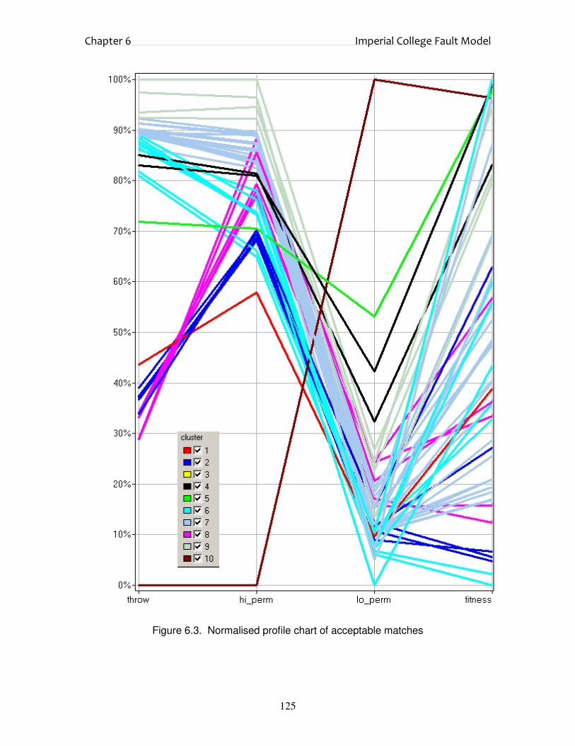
Chapter 6 Imperial College Fault Model
125
Figure 6.3. Normalised profile chart of acceptable matches
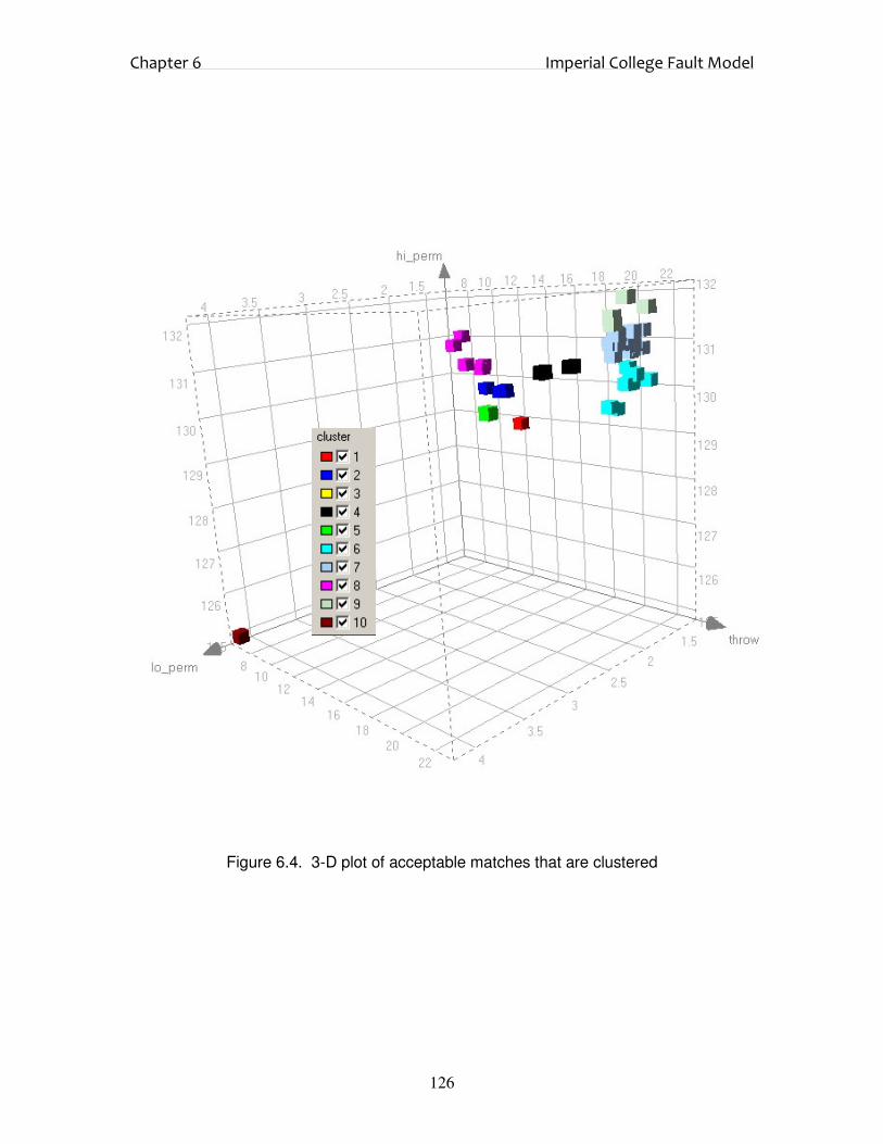
Chapter 6 Imperial College Fault Model
126
Figure 6.4. 3-D plot of acceptable matches that are clustered

Chapter 6 Imperial College Fault Model
127
The next step is to determine which members of each cluster to take into
forecasting. In this thesis a practical approach is taken, considering CPU
availability, disk space and most importantly time available to the engineer
for an uncertainty study task. In this regard, the minimum of each cluster is
only taken into a table for a final qualitative analysis as in Table 3.
It can be seen that there are still some similarities between the various
matches, though they appear distinctly different on Figure 6.3. This is
because Figure 6.3 is a normalised plot hence is very useful qualitatively, not
quantitatively. Similar matches are grouped in Table 6.1, and the minimums
of each group taken as the final set to carry forward into the prediction viz.
Match 2, 7, 9 and 10. It can be seen that Match 9 is very close to the truth
case, in fact the Flexi-PSO would be able to refine the match closer to the
truth case if the improvement tolerance is slackened before reinitialisation.

Chapter 6 Imperial College Fault Model
128
Throw Hi-perm Lo-perm Fitness
Truth 10.60 131.60 1.31 0.00
Match 1 20.41 130.44 1.50 1.67
Match 2 19.58 129.53 1.48 0.99
Match 3 20.25 130.69 2.21 2.62
Match 4 19.92 130.66 2.49 2.93
Match 5 17.91 129.86 2.17 2.86
Match 6 18.10 129.92 2.80 2.91
Match 7 22.66 131.99 2.05 2.58
Match 8 13.53 129.03 1.57 2.09
Match 9 11.13 130.98 1.99 1.73
Match 10 6.47 124.96 4.14 2.88
Table 6.1. List of final history matches
Figures 6.5-6.8 show the production plots for five years. The first three years
are the history match period and the last two years is the prediction phase.
Matches 1-10 were all carried through to check whether eliminating them
loses any valuable information. For the history match period the ensemble is
able to track the truth case well, and the final reduced set (in bold lines) is
adequate to capture the range of the ensemble. It must be noted from Figures
6.5 & 6.7 (oval demarcated area) that late in the prediction the ensemble is
not able to track the truth case. This is important as it makes one realize that
generating an ensemble is quite valuable to give an idea of the uncertainty
range but is by no means definitive.

Chapter 6 Imperial College Fault Model
129
Figure 6.5. Oil Production Rate
100
200
300
400
500
600
0 200 400 600 800 1000 1200 1400 1600 1800 2000
Days
Oil
Pro
du
cti
on
(b
bl/
d)
Truth Case
Match 1
Match 2
Match 3
Match 4
Match 5
Match 6
Match 7
Match 8
Match 9
Match 10

Chapter 6 Imperial College Fault Model
130
Figure 6.6. Cumulative Oil Production
0.E+00
1.E+05
2.E+05
3.E+05
4.E+05
5.E+05
6.E+05
7.E+05
8.E+05
9.E+05
1.E+06
0 200 400 600 800 1000 1200 1400 1600 1800 2000
Days
Cu
mu
lati
ve
Oil
Pro
du
cti
on
(b
bls
)
Truth Case
Match 1
Match 2
Match 3
Match 4
Match 5
Match 6
Match 7
Match 8
Match 9
Match 10

Chapter 6 Imperial College Fault Model
131
Figure 6.7. Water Production Rate
0
100
200
300
400
500
600
700
800
900
0 200 400 600 800 1000 1200 1400 1600 1800 2000
Days
Wa
ter
Pro
du
cti
on
(b
bls
/d)
Truth Case
Match 1
Match 2
Match 3
Match 4
Match 5
Match 6
Match 7
Match 8
Match 9
Match 10

Chapter 6 Imperial College Fault Model
132
Figure 6.8. Cumulative Water Production
0
50000
100000
150000
200000
250000
300000
350000
400000
450000
500000
0 200 400 600 800 1000 1200 1400 1600 1800 2000
Days
Cu
mu
lati
ve W
ate
r P
rod
ucti
on
(b
bls
)
Truth Case
Match 1
Match 2
Match 3
Match 4
Match 5
Match 6
Match 7
Match 8
Match 9
Match 10

Chapter 6 Imperial College Fault Model
133
Figure 6.9 illustrates the fitness history of the Flexi-PSO. It can be seen that
up to the 30th iteration the swarm converges very quickly but from here on
(oval demarcated area) there doesn’t appear to be any improvement in the
global best solution and in fact the swarm appears to be finding progressively
poorer solutions. This is due to the sequential niching nature of the Flexi-
PSO, where minima that have already been found have been isolated and as
the swarm is now exploring other areas of the search space it cannot find any
other reasonable minima.
Figure 6.9. Fitness history
0 5 10 15 20 25 30 35 40 45 500
50
100
150
200
250
iterations
fitn
ess
Flexi-PSO

Chapter 6 Imperial College Fault Model
134
The minimum fitness is obtained on the 24th iteration and is represented by
Match 2 (Table 6.1). Unlike any other method previously reported this
divergence is in fact an encouraging indicator because one now has the option
of stopping the global search procedure and complete the analysis of the
assisted history match. Finally one always has the option of taking this a
step further, time and resources permitting, to execute the cognition only
version of the PSO or a local search algorithm to fine tune the final set of
matches to see if any slightly better solution can be found.
A further attempt at history matching the ICF model using the Flexi-PSO
and function stretchingfunction stretchingfunction stretchingfunction stretching was investigated. This also serves to investigate the
effect on a different starting population on another run. The final list of
history matches is presented in Table 6.2. Distinct matches have been
isolated using this technique, but this time the niche containing the truth
case has not been found. Since function stretching elevates the fitness
landscape, niches with a narrow valley can be even more difficult to identify
as the stretching can lead to narrow needle like valleys in the transformed
fitness landscape. This also leads onto the conclusion that any uncertainty
modelling task should preferably be done with different starting populations
on different runs to ensure that the fitness landscape has been searched more
thoroughly.

Chapter 6 Imperial College Fault Model
135
Throw Hi-perm Lo-perm Fitness
Truth 10.60 131.60 1.31 0.00
Match 1 5.5064 119.82 9.9581 2.4606
Match 2 5.9013 120.47 9.5479 2.6728
Match 3 17.566 129.32 1.9041 1.6375
Match 4 17.586 129.39 2.1557 1.2772
Match 5 17.589 129.38 2.3202 2.0165
Match 6 17.59 129.37 4.3485 2.7946
Match 7 17.601 129.35 2.1453 1.325
Match 8 17.64 129.26 2.1185 1.5769
Match 9 17.765 128.96 2.0321 2.4119
Match 10 2.2419 121.61 2.9937 1.2027
Table 6.2. List of final history matches for function stretching transformation
Figure 6.10. Fitness history for function stretched transformation
0 5 10 15 20 25 30 35 40 45 500
50
100
150
200
250
iterations
fitn
ess

Chapter 6 Imperial College Fault Model
136
Figure 6.10 illustrates the fitness history of the function stretched
transformation. For scale purposes the true fitness values are plotted and not
the transformed fitness. Once the first niche is isolated at the 25th iteration,
successive niches are then visited as the model objective is transformed. This
is valuable as it directs the swarm fairly quickly to the non-transformed
areas. The drawback is that it is much more difficult to get into the niche
that contains the truth case since the transformation results in a very “spiky”
fitness landscape. In a multimodal landscape this will result in niches
residing in the spiked areas and hence being separated in a somewhat
discontinuous fashion. This would require many more iterations to find the
truth case as once the swarm finds the first niche, the objective function is
transformed and the swarm will then search for the next niche and once a
particle finds the next niche and the globalbest is updated, the rest of the
particles will rush into that niche without much exploration of the rest of the
search space since the contrast in fitness is so large.
This enhances the sequential niching nature of the Flexi-PSO but it does
mean that the more spikes there are in the objective transformation, the
longer it will take to find the region of the truth case as evidenced in this
study.

Chapter 6 Imperial College Fault Model
137
Using the Nelder-Mead Simplex direct search method (Lasgarias et al, 1998)
to history match the ICF Model makes a further test as to the efficiency of
the Flexi-PSO. A brief description of direct search was given in Chapter 1.2.
The FMINSEARCH option within MATLAB was employed for this task.
Since the original formulation of the Nelder-Mead technique was not
designed to handle bounds, direct usage of this option always led to solutions
outside the desired range of the uncertainty parameters.
A modified version FMINSEARCHBND (D’Errico, 2006) that is able to
handle boundary constraints by an internal transformation of the variables
(quadratic for single bounds, sin(x) for dual bounds) was then used to history
match the ICF Model. 10 attempts were made using random starting points
and each attempt was allowed 1000 function evaluations to be commensurate
with the Flexi-PSO. The results are shown in Table 6.3. Each attempt
terminated once the improvement in the objective function was less than the
specified tolerance that was set very low at 0.001 to allow
FMINSEARCHBND to make as many function evaluations as possible.
The resulting best fitness on all attempts was very poor and it is clear that
the Flexi-PSO outperforms it.

Chapter 6 Imperial College Fault Model
138
Throw Hi-perm Lo-perm Fitness fevals
Truth 10.60 131.60 1.31 0.00
Match 1 52.03 170.07 9.70 4.67 243
Match 2 49.56 162.02 9.70 4.98 303
Match 3 28.05 138.41 1.01 12.98 224
Match 4 54.16 174.61 11.78 4.64 252
Match 5 57.56 101.05 41.19 13.03 204
Match 6 12.33 136.00 1.22 18.16 175
Match 7 55.98 102.25 35.37 12.99 119
Match 8 55.98 180.29 13.33 4.53 184
Match 9 16.69 128.99 1.68 3.32 197
Match 10 47.10 152.41 2.82 11.16 216
Table 6.3. List of history matches from modified Nelder-Mead Simplex method

Chapter 7 North Sea Gasfield Case Study
139
Chapter 7
History Matching & Forecasting : Case Study of a
North Sea Gasfield
A North Sea Gasfield is now studied to check the effectiveness of the Flexi-
PSO and to further investigate the uncertainty evaluation conclusions of the
ICF model case study. It could be that since the ICF model has a very
difficult fitness landscape and quite a simple cross-sectional grid that the
uncertainty results are anomalous to it, hence further research into a real
field model is warranted.
A Gasfield that Shell operates in the North Sea is selected for this case study.
To be able to meaningfully assess the performance of the Flexi-PSO on
history matching this real field model, a set of modifiers and a respective set
of values are defined as the truth case for the model. The model is then run
for ~ 4 years and this production regarded as the truth case history. The
Flexi-PSO is then unleashed on the model modifiers with predefined ranges
and the fitness history is then analysed and clustered to isolate a final set of
matches to be taken into forecasting. A synthetic model like this is much
more useful than matching to true production data since there is no way of

Chapter 7 North Sea Gasfield Case Study
140
evaluating whether the forecasts from the matches obtained will in fact
encapsulate the true future production.
7.1. Field Description
This is a clastic reservoir with combined structural and stratigraphic traps.
There is some internal faulting but the faults do not compartmentalise the
reservoir. The sands were deposited in a sand-rich turbidite system. The
reservoir section is subdivided into 4 lithostratigraphic units (E – laterally
variable thin heterogeneous, D – laterally extensive massive sand, C –
laterally extensive mudstone rich heterogeneous & A – laterally restricted
sand rich) as in Figure 7.1. The bulk of the gas occurs in Unit D, which, with
high overall net/gross, porosity and permeability, has excellent reservoir
quality. The mud-rich Unit C is expected to mitigate against bottom-water
influx, so that most of the water drive is expected to come from edge aquifers.
The reservoir production mechanism is gas expansion drive supplemented by
aquifer influx.
The fluid is a fairly dry gas with very little liquid dropout at the facilities.
There are five vertical, partially penetrated wells, all completed in the E and
D units. In this study, a set of modifiers are taken as the truth case (Table

Chapter 7 North Sea Gasfield Case Study
141
7.1) which in fact reflect the real uncertainty in the field. The production
rates used in the history match are derived from the real production as well.
Figure 7.1. Lithostratigraphic x-section of the reservoir
Since primary depletion is the main drive mechanism, a pore volume
multiplier is applied to the synthetic case (PV mult). A vertical
transmissibility multiplier is also applied to the main D unit to accelerate the
flow vertically and exacerbate any effect of coning (CTRZ Dsand). An integer
variable is applied to the connectivity between the C & D units with the
default being no connectivity (CTR CD). Since gas expansion is the primary
drive mechanism, the connected volume would play an important role.
500 1000 1500 2000 2500 3000 3500 4000 4500 5000 5500 6000 6500 7000 7500 8000 8500 9000
500 1000 1500 2000 2500 3000 3500 4000 4500 5000 5500 6000 6500 7000 7500 8000 8500 9000
-10000
-9600
-9200
-8800
-8400
-8000
-7600
-10000
-9600
-9200
-8800
-8400
-8000
-7600
0 500 1000 1500 2000 2500m
1:40000
D
C
A
GWC
Well 1
Well 2Well 3
Well 5
Well 4
Well positions areprojected
E
500 1000 1500 2000 2500 3000 3500 4000 4500 5000 5500 6000 6500 7000 7500 8000 8500 9000
500 1000 1500 2000 2500 3000 3500 4000 4500 5000 5500 6000 6500 7000 7500 8000 8500 9000
-10000
-9600
-9200
-8800
-8400
-8000
-7600
-10000
-9600
-9200
-8800
-8400
-8000
-7600
0 500 1000 1500 2000 2500m
1:40000
D
C
A
GWC
Well 1
Well 2Well 3
Well 5
Well 4
Well positions areprojected
E
D
C
A
GWC
Well 1
Well 2Well 3
Well 5
Well 4
Well positions areprojected
E

Chapter 7 North Sea Gasfield Case Study
142
History Match Modifier
Min Max Truth
PV mult 0.8 1.2 0.9
CTRZ Dsand 20 50 45
CTR CD 0 1 0
AQFW Length 20000 50000 45000
AQFE Length 15000 35000 20000
AQFW Perm 50 300 250
AQFE Perm 400 800 650
Rock Compr. 2e-6 5e-6 3e-6
Res. Gas 0.1 0.25 0.14
Table 7.1. History Match Modifiers and their range
There are linear finite analytical aquifers attached to the grid on the western
and eastern flanks of the field and their respective lengths and permeabilities
are a source of uncertainty (AQFW Length, AQFE Length, AQFW Perm,
AQFE Perm). Rock compressibility is thrown into the history match as a red
herring to test whether the Flexi-PSO would concentrate its efforts on this
variable. Finally the residual gas saturation is added to add to the effect of
the primary drive mechanism as it affects the movable gas volumes. The
simulator automatically scales the relative permeability according to
whatever residual gas saturation is specified at initialisation.
A One-Parameter-at-a-Time (OPAT) sensitivity test is run on all the
variables to get an initial gauge of the effect of each variable on the gas
production. Figure 7.2 displays the tornado chart for this sensitivity analysis

Chapter 7 North Sea Gasfield Case Study
143
where the base case is taken as the mid-point of the modifier range. The
production is especially sensitive to the pore volume multiplier and
intuitively this makes sense as the gas volume is the main driving force in
the system. The connectivity of the C & D units also appears to play a role, as
this naturally would add more connected volume to the system.
Figure 7.2. Tornado plot of OPAT sensitivity
The Faure Sequence presented in Chapter 6.1 is also useful as a designed
experiment (since they are evenly space filling) to quickly screen variables
and have a relative idea of their effect. Trends in the effect of variables can
also be ascertained and variables with little/no effect can be discarded at this
-150 -100 -50 0 50 100 150
Res. Gas
AQFW Length
AQFE Perm
CTRZ Dsand
AQFW Perm
CTR_CD
Rock Compr
AQFE Length
PVmult
delta CGP (Bscf)

Chapter 7 North Sea Gasfield Case Study
144
stage. To this end, one hundred runs were set up within the ranges specified
in Table 7.1. Figure 7.3 shows the results of these runs.
Figure 7.3. Faure Sequence “designed experiment”
Figure 7.4 plots the relative effect of each variable on the fitness using the
well known correlation function (7.1.1) (µ - mean, σ- standard deviation).
0.8 0.9 1 1.1 1.20
5
10
15
20
Fitness
PV mult
20 30 40 500
5
10
15
20
Fitness
CTRZ Dsand
0 0.5 10
5
10
15
20
Fitness
CTR CD
2 3 4 5
x 104
0
5
10
15
20
Fitness
AQFW Length
1.5 2 2.5 3 3.5
x 104
0
5
10
15
20
Fitness
AQFE Length
50 100 150 200 250 3000
5
10
15
20
Fitness
AQFW PERM
400 500 600 700 8000
5
10
15
20
Fitness
AQFE PERM
2 3 4 5
x 10-6
0
5
10
15
20
Fitness
Rock Compr
0.1 0.15 0.2 0.250
5
10
15
20
Fitness
Res Gas
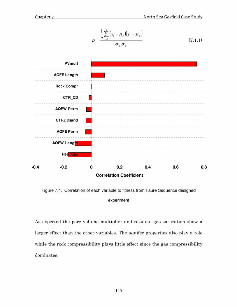
Chapter 7 North Sea Gasfield Case Study
145
( )( )
yx
n
i
yixi yxn
σσ
µµ
ρ.
1
1
∑=
−−
= (7.1.1)
Figure 7.4. Correlation of each variable to fitness from Faure Sequence designed
experiment
As expected the pore volume multiplier and residual gas saturation show a
larger effect than the other variables. The aquifer properties also play a role
while the rock compressibility plays little effect since the gas compressibility
dominates.
-0.4 -0.2 0 0.2 0.4 0.6 0.8
Res. Gas
AQFW Length
AQFE Perm
CTRZ Dsand
AQFW Perm
CTR_CD
Rock Compr
AQFE Length
PVmult
Correlation Coefficient

Chapter 7 North Sea Gasfield Case Study
146
There are ~ 170 000 gridblocks in the model with ~ 53 000 active. Figure 7.5
is a water saturation gridview of the model at an arbitrary point in time.
Figure 7.5. Overall Sw gridview of the model
7.2. Results and Discussion
The simulator used is MoReS (Shell proprietary). The Flexi-PSO was set up
in the same way as in the ICF Model case study with a population of 20
particles and 50 iterations. Each run took about three hours and distributed
over a cluster of CPU’s the entire Flexi-PSO run took six days to complete.
W3 W4
W2
W5
W1
N

Chapter 7 North Sea Gasfield Case Study
147
All matches with RMSE less than 1 were considered acceptable from a visual
judgement of the history match versus production plots. There were 50
acceptable matches, which were then clustered into 10 groups using average
linkage hierarchical clustering. The match with the lowest fitness in each
group was then taken forward into forecasting. Table 7.2 presents these final
matches.
It is encouraging to note that the Flexi-PSO has performed well on this
mixed-integer problem with all the acceptable matches having no
transmissibility between the C & D units as in the truth case.
PVmult CTRZ Dsand
CTR_CD AQFW Length
AQFE Length
AQFW Perm
AQFE Perm
Rock Compr
Res. Gas Fitness
Truth 0.9 45 0 45000 20000 250 650 3e-6 0.14 0
Match 1 0.952 29.46 0 41249 34384 116.14 465.71 4.26E-06 0.158 0.813
Match 2 0.943 23.92 0 43293 25611 104.46 518.18 4.48E-06 0.151 0.239
Match 3 0.940 27.09 0 47665 29593 112.41 514.12 3.51E-06 0.135 0.317
Match 4 0.940 28.71 0 39158 24162 155.06 588.34 3.67E-06 0.164 0.768
Match 5 0.951 34.01 0 28844 23173 98.62 634.53 4.14E-06 0.176 0.526
Match 6 0.935 35.76 0 26781 23856 163.16 566.98 3.94E-06 0.166 0.439
Match 7 0.962 22.15 0 30491 33770 119.33 546.00 3.87E-06 0.150 0.932
Match 8 0.964 39.58 0 21796 28192 105.20 561.41 4.13E-06 0.200 0.871
Match 9 0.948 21.59 0 27098 22328 131.82 756.51 3.77E-06 0.158 0.887
Match 10 0.930 25.44 0 25547 22377 235.35 732.47 2.72E-06 0.168 0.771
Table 7.2. Final set of history matched models

Chapter 7 North Sea Gasfield Case Study
148
Figure 7.6 displays the fitness history of the Flexi-PSO. The restarts are
highlighted where the sequential niching process takes effect. The range of
each niche is set to 10% of the dynamic range for each modifier. In this run
there have been three restarts of the algorithm. On each restart the
algorithm does reduce the fitness rapidly but still explores the search space.
Figure 7.6. Fitness history of the Flexi-PSO ( x – globalbest tracker in each niche
sequence )
Figures 7.7 - 7.12 display the history match per well and field for each
realisation. The history period starts at 01/11/2004 and ends at 01/03/2008
0 5 10 15 20 25 30 35 40 45 500
5
10
15
20
25
30
Iterations
Fit
ness

Chapter 7 North Sea Gasfield Case Study
149
(demarcated on each plot). The forecast ends at 01/01/2011. To make the
forecasting more challenging in terms of uncertainty modelling, it is assumed
that the production facilities can no longer handle any more water
throughput. In this way, the forecasts can now be analysed with respect to
the truth case to see whether they do encapsulate it and if so, how wide is the
forecasted uncertainty band. The forecast has a surface pipeline network
with a compressor attached to it. The compression logic built into the deck
states that whenever the tubing head pressure drops below a certain
threshold, the compressor speed is then ramped up to compensate for this
pressure drop which in turn leads to an increase in production.
Figure 7.7 shows the matches to Well 1 to be acceptable. Each match is able
to produce the rates and track the flowing bottomhole pressure. The truth
case forecast for this well is interesting as it is around 20 Bscf away from the
ensemble as the truth case produces for a much longer duration that the rest
of the cases. In Figure 7.8, the matches to Well 2 are also acceptable, with the
flowing bottomhole pressure being tracked quite nicely. This well shuts in at
the end of 2008 and hence its no surprise then that the ensemble does
capture the truth case for the cumulative production for this well. In Figure
7.9, the matches to Well 3 are all acceptable with a slight deviation of the
ensemble to the flowing bottomhole pressure near the end of history. The

Chapter 7 North Sea Gasfield Case Study
150
truth case for this well shuts in before the rest of the ensemble and hence has
a cumulative production below the range of the ensemble.
In Figure 7.10, Well 4 has acceptable matches to the gas production and
bottomhole pressure. This is the only well in the history that does produce
water and its water production rate is in Figure 7.10. The ensemble does
encapsulate the water production, but there is quite a wide uncertainty band
(~ 3400 bbl/d to ~ 4200 bbl/d). In Figure 7.11, Well 5 has acceptable matches
with the flowing bottomhole pressure deviating slightly towards the end of
the history. The truth case shuts in before the rest of the ensemble and hence
this well has a cumulative production that is lower than the ensemble. All
the wells show an upturn in the bottomhole pressure towards the end of the
forecast. This is due to the continuous charging of the reservoir from the
aquifers.
In Figure 7.12, the ensemble does encapsulate the cumulative field
production but not the field rate. This is because Well 1 continues to produce
much later in the truth case than the history match cases. The results of this
gasfield study are in stark similarity to that obtained with the ICF Model.
Once again, we are faced with the likelihood that the ensemble will not be
able to encapsulate the range on the production rate, but for the field as a

Chapter 7 North Sea Gasfield Case Study
151
whole it is more likely that the ensemble will encapsulate the truth case for
the cumulative production. The reason for this is simple.
Lets assume we have a set of realisations, the only difference between them
being pore volume multipliers while all other parameters are held constant.
In this case, when the realisations are simulated the “likely outcome” will be
a forecast range that is proportional to the pore volume multipliers. If we
have a set of realisations that have similar volumes but differing properties,
the “likely outcome” is that they will all produce similar forecasts in terms of
the overall volume drained from the reservoir. As in this North Sea Gasfield
study, the truth case sees Well 2 and Well 3 water out earlier than the
history matches, but Well 1 sees more production than the history match
cases as it now has a greater volume available to drain. Hence the reason for
the fairly tight forecast envelope on the cumulative gas production.
It is important to note here that even with a perfect structural model, correct
set of uncertainty parameters, ranges that cover the truth case and perfect
measurements, as well as a set of excellent history matches, that the truth
case production still cannot be encapsulated for the wells when forecasting!
This makes the case for using uncertainty modelling to identify infill drilling
targets somewhat tenuous. (Millar, 2005) quotes an example of an oil major
identifying an infill location as being better than two other targets with

Chapter 7 North Sea Gasfield Case Study
152
similar average cumulative production because its forecast envelope was
narrower. If as shown in this North Sea Gasfield case study, producing wells
with a good set of matches and modifiers that are appropriately conditioned
to historical production cannot encapsulate the truth case production for a
gasfield, it hardly seems plausible that an infill location for an oil well (where
relative permeability effects are more pronounced) can be identified to be
better than any other location with similar production but a narrower
forecast envelope.

Chapter 7 North Sea Gasfield Case Study
153
Figure 7.7. Well 1 matches (QGP – mmscfd, CGP - bscf, BHP - psia)

Chapter 7 North Sea Gasfield Case Study
154
Figure 7.8. Well 2 matches (QGP – mmscfd, CGP - bscf, BHP- psia)

Chapter 7 North Sea Gasfield Case Study
155
Figure 7.9. Well 3 matches (QGP – mmscfd, CGP - bscf, BHP - psia)

Chapter 7 North Sea Gasfield Case Study
156
Figure 7.10. Well 4 matches (QGP – mmscfd, CGP - bscf, BHP - psia, QWP – bbl/d)

Chapter 7 North Sea Gasfield Case Study
157
Figure 7.11. Well 5 matches (QGP – mmscfd, CGP - bscf, BHP - psia)

Chapter 7 North Sea Gasfield Case Study
158
Figure 7.12. Field matches (QGP – mmscfd, CGP - bscf, QWP – bbl/d, CWP - mbbl/d )

CONCLUSIONS

Conclusions
160
Chapter 8
Conclusions
The theme of this thesis has been to examine key issues that we are faced
with in history matching and try to develop an effective workflow in the
history matching process that will generate meaningful results to practising
reservoir engineers. In this regard, the focus is on further advancements in
the area of assisted history matching. The key areas that this thesis
contributes to can be summarised as follows :-
• Introduction of Particle Swarm Optimisation to the oil industry
• Understanding the effects of the parameters in the Particle Swarm
Optimiser
• Development of a state of the art variant of the Particle Swarm
Optimisation algorithm for history matching purposes (Flexi-PSO)
• Techniques of post-processing an assisted history match run
• Insight into the possible implications of the results of an uncertainty
modelling exercise
Particle Swarms are a novel optimisation technique and are used in this
thesis to history match finite difference reservoir simulation models. Particle

Conclusions
161
Swarms form part of the so-called evolutionary class of optimization
algorithms that are population based and use various communication
mechanisms to move towards optimal solutions. This is the first known
implementation of particle swarms in the oil and gas industry and has been
successfully applied to the Imperial College Fault Model to locate distinctly
different history matches.
Particle swarms if designed properly can be very effective in moving through
the search space and are effective in balancing global exploration and local
exploitation. In this regard, a particle swarm variant dubbed “Flexi-PSO” has
been specifically created that can quickly locate multiple niches and also
handle multiple static realisations or discrete parameters. The motto behind
the Flexi-PSO is “Big moves coupled with small moves”. This theme enables
the swarm to scan niches more thoroughly and the reason behind its success
in dealing with benchmark mathematical functions and the history matching
case studies presented. The reason for this is that in the canonical and
inertia weight versions of the PSO, particles concentrate on doing a global
search and have high velocities from the outset which can lead to a particle
that may be in a niche that contains the global optimum to fly out of that
region. The Flexi-PSO reduces that possibility by enabling particles to also
make local searches during the course of the run.

Conclusions
162
Before any optimisation algorithm can be deployed, it is best to test it against
a wide range of problems to assess its robustness, and in doing so any
shortcomings of the algorithm can be addressed. This thesis interrogated the
Flexi-PSO with convex and highly non-convex mathematical functions, a
neural network and integer problems. The Flexi-PSO is shown to have
comparative efficacy as current state of the art algorithms. The algorithm is
further modified to increase its effectiveness in dealing with multimodal
problems via a sequential niching routine, which has shown to be effective in
locating multiple optima.
The Flexi-PSO is then used to history match the Imperial College Fault
Model and returns a match that is very close to the truth case, however this
is not the case on every single run as was shown when function stretching
was applied to niches. The results of the history matching procedure do
require some post processing. A simple graphical approach combined with
hierarchical clustering can be used to narrow down a final set of realizations
to carry forward into prediction.
Even with the best algorithms and methods of processing results, it is still
imperative to understand that the model is not a perfect reflection of the
reservoir properties. This thesis shows that even with a highly effective
algorithm like the “Flexi-PSO”, the ensemble of matches that we are left with

Conclusions
163
(even with one match that is very close to the truth case), there is no
guarantee that their predictions will cover the true reservoir behaviour.
It is useful that unlike unstable systems in chaos theory which have a
multiplicative effect if the starting point is incorrect and leads to less
accurate behaviour over time, petroleum reservoirs are dissipative in energy
and cumulative production predictions tend to flatten out the longer the
prediction is in time. In this regard an ensemble is likely to create a
prediction envelope that will cover the truth case with regards to field
cumulative production (provided that the initial volumes in place are
representative), however it is less likely that it will do so for well production
rates.
The Flexi-PSO is then used to history match a synthetic version of a North
Sea Gasfield. The results of this case study are indeed very interesting.
Although the Flexi-PSO has successfully managed to find multiple matched
cases, the matched cases in fact point to an interesting insight into
evaluating uncertainty. All the history match cases have similar volumes in
place and their narrow forecast range does encapsulate the cumulative
production of the truth case. However, as was observed in the ICF Model case
study, the same cannot be said of the production rate. It becomes even more
interesting on a well level, where we see that it is much more difficult for the

Conclusions
164
ensemble to track the truth case production. In this case where wells are
being shut in due to the limit on the water handling capacity, the remaining
gas volume is then left available for other wells to drain.
Essentially, it appears that the wider the hydrocarbon in place volume range
there is from a set of history match realisations, the wider it can be expected
the reserves forecast will be. For a narrow in place volume range, the wells
will compete for production and wells that are shut-in will just leave more
volume for the remaining wells to access.
As shown in the North Sea Gasfield case study, producing wells with a good
set of matches and modifiers that are appropriately conditioned to historical
production cannot encapsulate the truth case for a gasfield, it hardly seems
plausible that an infill location for an oil well can be identified to be better
than any other location with similar production but a narrower forecast
envelope. This criteria needs to reviewed very carefully, and other
environmental factors should be called into account e.g. drilling cost when
making a final decision.
In short any history matching exercise requires a good optimisation
algorithm together with post processing of results to take meaningful
realisations forward into prediction. The end result is as is commonly

Conclusions
165
quipped only as good as the model itself, hence some degree of common sense
needs to be exercised in the allocation of time and resources with respect to
any history matching exercise.

Appendix
166
APPENDIX

Appendix A CEC-2005 Testset
167
Appendix A
Problem Definitions for the CEC 2005 Special Session
on Real-Parameter Optimisation
Summary of the 25 Test Functions
� Unimodal Functions (5):
� F1: Shifted Sphere Function
� F2: Shifted Schwefel’s Problem 1.2
� F3: Shifted Rotated High Conditioned Elliptic Function
� F4: Shifted Schwefel’s Problem 1.2 with Noise in Fitness
� F5: Schwefel’s Problem 2.6 with Global Optimum on Bounds
� Multimodal Functions (20):
� Basic Functions (7):
� F6: Shifted Rosenbrock’s Function
� F7: Shifted Rotated Griewank’s Function without Bounds
� F8: Shifted Rotated Ackley’s Function with Global Optimum on
Bounds
� F9: Shifted Rastrigin’s Function
� F10: Shifted Rotated Rastrigin’s Function
� F11: Shifted Rotated Weierstrass Function
� F12: Schwefel’s Problem 2.13

Appendix A CEC-2005 Testset
168
� Expanded Functions (2):
� F13: Expanded Extended Griewank’s plus Rosenbrock’s Function
(F8F2)
� F14: Shifted Rotated Expanded Scaffer’s F6
� Hybrid Composition Functions (11):
� F15: Hybrid Composition Function
� F16: Rotated Hybrid Composition Function
� F17: Rotated Hybrid Composition Function with Noise in Fitness
� F18: Rotated Hybrid Composition Function
� F19: Rotated Hybrid Composition Function with a Narrow Basin for
the Global Optimum
� F20: Rotated Hybrid Composition Function with the Global Optimum
on the Bounds
� F21: Rotated Hybrid Composition Function
� F22: Rotated Hybrid Composition Function with High Condition
Number Matrix
� F23: Non-Continuous Rotated Hybrid Composition Function
� F24: Rotated Hybrid Composition Function
� F25: Rotated Hybrid Composition Function without Bounds

Appendix A CEC-2005 Testset
169
Unimodal Functions
F1: Shifted Sphere Function
2
1 1
1
( ) _D
i
i
F z f bias=
= +∑x , = −z x o , 1 2[ , ,..., ]D
x x x=x
D: dimensions. 1 2[ , ,..., ]D
o o o=o : the shifted global optimum.
Figure A-1. 3-D map for 2-D function
Properties:
� Unimodal
� Shifted
� Separable
� Scalable
� [ 100,100]D∈ −x , Global optimum: * =x o , 1( *)1
F f_bias=x = - 450
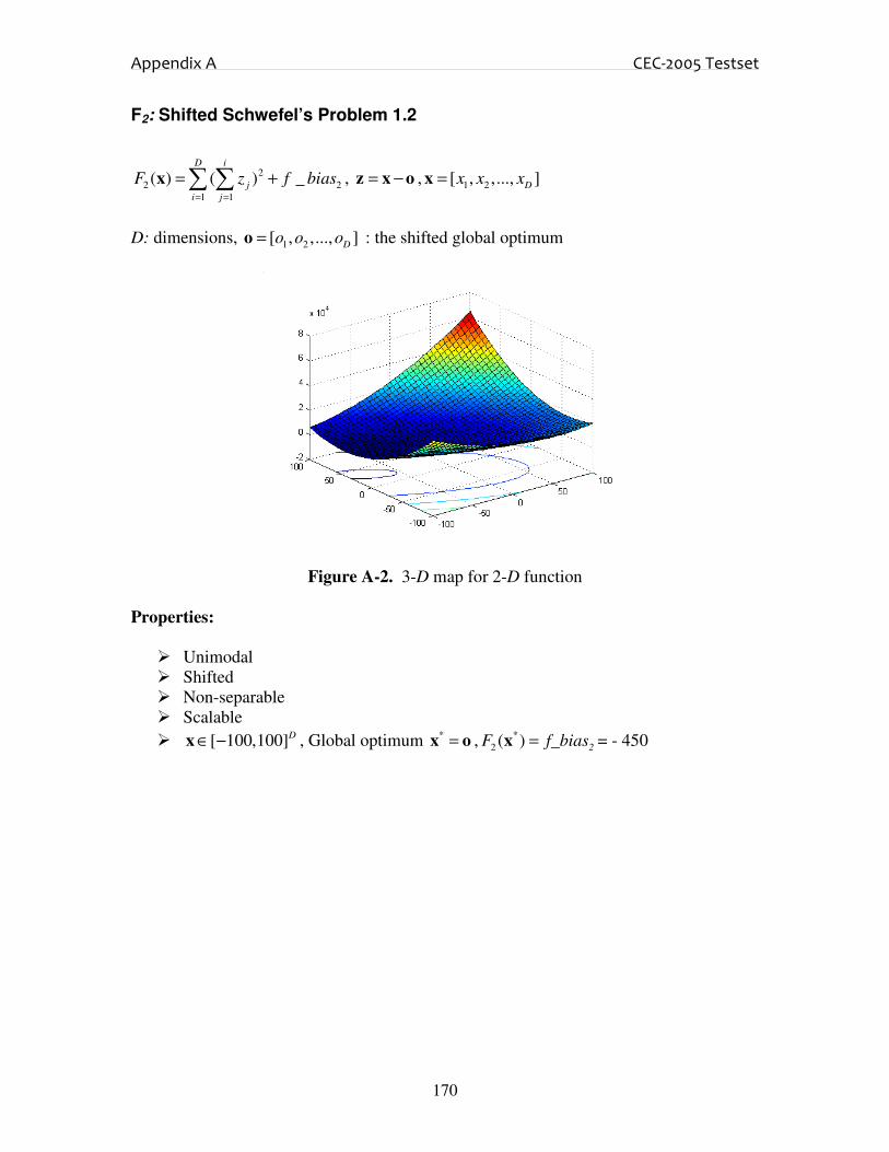
Appendix A CEC-2005 Testset
170
F2: Shifted Schwefel’s Problem 1.2
2
2 2
1 1
( ) ( ) _D i
j
i j
F z f bias= =
= +∑ ∑x , = −z x o , 1 2[ , ,..., ]D
x x x=x
D: dimensions, 1 2[ , ,..., ]D
o o o=o : the shifted global optimum
Figure A-2. 3-D map for 2-D function
Properties:
� Unimodal
� Shifted
� Non-separable
� Scalable
� [ 100,100]D∈ −x , Global optimum * =x o , *
2 ( )2
F f_bias=x = - 450

Appendix A CEC-2005 Testset
171
F3: Shifted Rotated High Conditioned Elliptic Function
1
6 213 3
1
( ) (10 ) _iD
Di
i
F z f bias−
−
=
= +∑x , ( )*= −z x o M , 1 2[ , ,..., ]D
x x x=x
D: dimensions, 1 2[ , ,..., ]D
o o o=o : the shifted global optimum
M: orthogonal matrix
Figure A-3. 3-D map for 2-D function
Properties:
� Unimodal
� Shifted
� Rotated
� Non-separable
� Scalable
� [ 100,100]D∈ −x , Global optimum * =x o , *
3( )3
F f_bias=x =- 450

Appendix A CEC-2005 Testset
172
F4: Shifted Schwefel’s Problem 1.2 with Noise in Fitness
2
4 4
1 1
( ) ( ( ) )*(1 0.4 (0,1) ) _D i
j
i j
F z N f bias= =
= + +∑ ∑x , = −z x o , 1 2[ , ,..., ]D
x x x=x
D: dimensions, 1 2[ , ,..., ]D
o o o=o : the shifted global optimum
Figure A-4. 3-D map for 2-D function
Properties:
� Unimodal
� Shifted
� Non-separable
� Scalable
� Noise in fitness
� [ 100,100]D∈ −x , Global optimum * =x o , *
4 ( )4
F f_bias=x = - 450

Appendix A CEC-2005 Testset
173
F5: Schwefel’s Problem 2.6 with Global Optimum on Bounds
1 2 1 2( ) max{ 2 7 , 2 5}, 1,...,f x x x x i n= + − + − =x , * [1,3]=x , *( ) 0f =x
Extend to D dimensions:
5 5( ) max{ } _ , 1,...,i iF f bias i D= − + =x A x B , 1 2[ , ,..., ]D
x x x=x
D: dimensions
A is a D*D matrix, ij
a are integer random numbers in the range [-500, 500],
det( ) 0≠A , Ai is the ith
row of A.
*i i
=B A o , o is a D*1 vector, i
o are random number in the range [-100,100]
set 100i
o = − , for 1,2,..., / 4i D= , 100i
o = ,for 3 / 4 ,...,i D D=
Figure A-5. 3-D map for 2-D function
Properties:
� Unimodal
� Non-separable
� Scalable
� If the initialization procedure initializes the population at the bounds, this problem
will be solved easily.
� [ 100,100]D∈ −x , Global optimum * =x o , *
5 ( )5
F f_bias=x = - 310

Appendix A CEC-2005 Testset
174
Basic Multimodal Functions
F6: Shifted Rosenbrock’s Function
1
2 2 2
6 1 6
1
( ) (100( ) ( 1) ) _D
i i i
i
F z z z f bias−
+=
= − + − +∑x , 1= − +z x o , 1 2[ , ,..., ]D
x x x=x
D: dimensions, 1 2[ , ,..., ]D
o o o=o : the shifted global optimum
Figure A-6. 3-D map for 2-D function
Properties:
� Multi-modal
� Shifted
� Non-separable
� Scalable
� Having a very narrow valley from local optimum to global optimum
� [ 100,100]D∈ −x , Global optimum * =x o , *
6 ( )6
F f_bias=x = 390

Appendix A CEC-2005 Testset
175
F7: Shifted Rotated Griewank’s Function without Bounds
2
7 7
1 1
( ) cos( ) 1 _4000
DDi i
i i
z zF f bias
i= =
= − + +∑ ∏x , ( )*= −z x o M , 1 2[ , ,..., ]D
x x x=x
D: dimensions
1 2[ , ,..., ]D
o o o=o : the shifted global optimum
M’: linear transformation matrix, condition number=3
M =M’(1+0.3|N(0,1)|)
Figure A-7. 3-D map for 2-D function
Properties:
� Multi-modal
� Rotated
� Shifted
� Non-separable
� Scalable
� No bounds for variables x
� Initialize population in [0,600]D , Global optimum * =x o is outside of the
initialization range, *
7 ( )7
F f_bias=x = -180

Appendix A CEC-2005 Testset
176
F8: Shifted Rotated Ackley’s Function with Global Optimum on Bounds
2
8 8
1 1
1 1( ) 20exp( 0.2 ) exp( cos(2 )) 20 _
D D
i i
i i
F z z e f biasD D
π= =
= − − − + + +∑ ∑x ,
( )*= −z x o M , 1 2[ , ,..., ]D
x x x=x , D: dimensions
1 2[ , ,..., ]D
o o o=o : the shifted global optimum;
After load the data file, set 2 1 32j
o − = − 2 jo are randomly distributed in the search range,
for 1, 2,..., / 2j D=
M: linear transformation matrix, condition number=100
Figure A-8. 3-D map for 2-D function
Properties:
� Multi-modal
� Rotated
� Shifted
� Non-separable
� Scalable
� A’s condition number Cond(A) increases with the number of variables as 2( )O D
� Global optimum on the bound
� If the initialization procedure initializes the population at the bounds, this problem
will be solved easily.
� [ 32,32]D∈ −x , Global optimum * =x o , *
8 ( )8
F f_bias=x = - 140

Appendix A CEC-2005 Testset
177
F9: Shifted Rastrigin’s Function
2
9 9
1
( ) ( 10cos(2 ) 10) _D
i i
i
F z z f biasπ=
= − + +∑x , = −z x o , 1 2[ , ,..., ]D
x x x=x
D: dimensions, 1 2[ , ,..., ]D
o o o=o : the shifted global optimum
Figure A-9. 3-D map for 2-D function
Properties:
� Multi-modal
� Shifted
� Separable
� Scalable
� Local optima’s number is huge
� [ 5,5]D∈ −x , Global optimum * =x o , *
9 ( )9
F f_bias=x = - 330

Appendix A CEC-2005 Testset
178
F10: Shifted Rotated Rastrigin’s Function
2
10 10
1
( ) ( 10cos(2 ) 10) _D
i i
i
F z z f biasπ=
= − + +∑x , ( )*= −z x o M , 1 2[ , ,..., ]D
x x x=x
D: dimensions, 1 2[ , ,..., ]D
o o o=o : the shifted global optimum
M: linear transformation matrix, condition number=2
Figure A-10. 3-D map for 2-D function
Properties:
� Multi-modal
� Shifted
� Rotated
� Non-separable
� Scalable
� Local optima’s number is huge
� [ 5,5]D∈ −x , Global optimum * =x o , *
10 ( )10
F f_bias=x = - 330

Appendix A CEC-2005 Testset
179
F11: Shifted Rotated Weierstrass Function
max max
11 11
1 0 0
( ) ( [ cos(2 ( 0.5))]) [ cos(2 0.5)] _D k k
k k k k
i
i k k
F a b z D a b f biasπ π= = =
= + − ⋅ +∑ ∑ ∑x ,
a=0.5, b=3, kmax=20, ( )*= −z x o M , 1 2[ , ,..., ]D
x x x=x
D: dimensions, 1 2[ , ,..., ]D
o o o=o : the shifted global optimum
M: linear transformation matrix, condition number=5
Figure A-11. 3-D map for 2-D function
Properties:
� Multi-modal
� Shifted
� Rotated
� Non-separable
� Scalable
� Continuous but differentiable only on a set of points
� [ 0.5,0.5]D∈ −x , Global optimum * =x o , *
11( )11
F f_bias=x = 90

Appendix A CEC-2005 Testset
180
F12: Schwefel’s Problem 2.13
2
12 12
1
( ) ( ( )) _D
i i
i
F f bias=
= − +∑x A B x , 1 2[ , ,..., ]D
x x x=x
1
( sin cos )D
i ij j ij j
j
a bα α=
= +∑A ,1
( ) ( sin cos )D
i ij j ij j
j
x a x b x=
= +∑B , for 1,...,i D=
D: dimensions
A, B are two D*D matrix, ij
a ,ij
b are integer random numbers in the range [-100,100],
1 2[ , ,..., ]D
α α α=αααα ,j
α are random numbers in the range [ , ]π π− .
Figure A-12. 3-D map for 2-D function
Properties:
� Multi-modal
� Shifted
� Non-separable
� Scalable
� [ , ]Dπ π∈ −x , Global optimum * =x αααα , *
12 ( )12
F f_bias=x = - 460

Appendix A CEC-2005 Testset
181
Expanded Functions
Using a 2-D function ( , )F x y as a starting function, corresponding expanded function is:
1 2 1 2 2 3 1 1( , ,..., ) ( , ) ( , ) ... ( , ) ( , )D D D D
EF x x x F x x F x x F x x F x x−= + + + +
F13: Shifted Expanded Griewank’s plus Rosenbrock’s Function (F8F2)
F8: Griewank’s Function: 2
1 1
8( ) cos( ) 14000
DDi i
i i
x xF
i= =
= − +∑ ∏x
F2: Rosenbrock’s Function: 1
2 2 2
1
1
2( ) (100( ) ( 1) )D
i i i
i
F x x x−
+=
= − + −∑x
1 2 1 2 2 3 1 18 2( , ,..., ) 8( 2( , )) 8( 2( , )) ... 8( 2( , )) 8( 2( , ))D D D D
F F x x x F F x x F F x x F F x x F F x x−= + + + +
Shift to
13 1 2 2 3 1 1 13( ) 8( 2( , )) 8( 2( , )) ... 8( 2( , )) 8( 2( , )) _D D D
F F F z z F F z z F F z z F F z z f bias−= + + + + +x
1= − +z x o , 1 2[ , ,..., ]D
x x x=x
D: dimensions 1 2[ , ,..., ]D
o o o=o : the shifted global optimum
Figure A-13. 3-D map for 2-D function
Properties:
� Multi-modal
� Shifted
� Non-separable
� Scalable
� [ 3,1]D∈ −x , Global optimum * =x o , *
13( )13
F f_bias=x (13)=-130

Appendix A CEC-2005 Testset
182
F14: Shifted Rotated Expanded Scaffer’s F6 Function
2 2 2
2 2 2
(sin ( ) 0.5)( , ) 0.5
(1 0.001( ))
x yF x y
x y
+ −= +
+ +
Expanded to
14 1 2 1 2 2 3 1 1 14( ) ( , ,..., ) ( , ) ( , ) ... ( , ) ( , ) _D D D D
F EF z z z F z z F z z F z z F z z f bias−= = + + + + +x ,
( )*= −z x o M , 1 2[ , ,..., ]D
x x x=x
D: dimensions, 1 2[ , ,..., ]D
o o o=o : the shifted global optimum
M: linear transformation matrix, condition number=3
Figure A-14. 3-D map for 2-D function
Properties:
� Multi-modal
� Shifted
� Non-separable
� Scalable
� [ 100,100]D∈ −x , Global optimum * =x o , *
14 ( )14
F f_bias=x (14)= -300

Appendix A CEC-2005 Testset
183
Composition functions
( )F x : new composition function
( )i
f x : ith
basic function used to construct the composition function
n : number of basic functions
D : dimensions
iM : linear transformation matrix for each ( )
if x
io : new shifted optimum position for each ( )
if x
1
( ) { *[ '(( ) / * ) ]} _n
i i i i i
i
F w f bias f biasλ=
= − + +∑x x o Mi
iw : weight value for each ( )
if x , calculated as below:
2
1
2
( )
exp( )2
D
k ik
k
i
i
x o
wDσ
=
−
= −∑
,
max( )
*(1-max( ).^10) max( )
i i i
i
i i i i
w w ww
w w w w
===
≠
then normalize the weight 1
/n
i i i
i
w w w=
= ∑
iσ : used to control each ( )
if x ’s coverage range, a small
iσ give a narrow range for that
( )i
f x
iλ : used to stretch compress the function,
iλ >1 means stretch,
iλ <1 means compress
oi define the global and local optima’s position,
ibias define which optimum is global
optimum. Using oi,
ibias , a global optimum can be placed anywhere.
If ( )i
f x are different functions, different functions have different properties and height,
in order to get a better mixture, estimate a biggest function value max i
f for 10 functions
( )i
f x , then normalize each basic functions to similar heights as below:
max'( ) * ( ) /i i if C f f=x x , C is a predefined constant.
max if is estimated using max if = (( '/ )* )i i i
f λx M , 'x =[5,5…,5].
In the following composition functions,
Number of basic functions n=10.
D: dimensions
o: n*D matrix, defines ( )i
f x ’s global optimal positions
bias =[0, 100, 200, 300, 400, 500, 600, 700, 800, 900]. Hence, the first function1( )f x
always the function with the global optimum.
C=2000

Appendix A CEC-2005 Testset
184
Pseudo Code:
Define f1-f10, σ , λ , bias, C, load data file o and rotated linear transformation matrix
M1-M10
y =[5,5…,5].
For i=1:10
2
1
2
( )
exp( )2
D
k ik
k
i
i
x o
wDσ
=
−
= −∑
,
((( ) / )* )i i i i i
fit f λ= −x o M
max (( / )* )i i i i
f f λ= y M ,
* / maxi i i
fit C fit f=
EndFor
1
n
i
i
SW w=
=∑
max( )i
MaxW w=
For i=1:10
*(1- .^10)
i i
i
i i
w if w MaxWw
w MaxW if w MaxW
===
≠
/i i
w w SW=
EndFor
1
( ) { *[ ]}n
i i i
i
F w fit bias=
= +∑x
( ) ( ) _F F f bias= +x x

Appendix A CEC-2005 Testset
185
F15: Hybrid Composition Function
1 2( )f − x : Rastrigin’s Function
2
1
( ) ( 10cos(2 ) 10)D
i i i
i
f x xπ=
= − +∑x
3 4( )f − x : Weierstrass Function
max max
1 0 0
( ) ( [ cos(2 ( 0.5))]) [ cos(2 0.5)]D k k
k k k k
i i
i k k
f a b x D a bπ π= = =
= + − ⋅∑ ∑ ∑x ,
a=0.5, b=3, kmax=20
5 6( )f − x : Griewank’s Function
2
1 1
( ) cos( ) 14000
DDi i
i
i i
x xf
i= =
= − +∑ ∏x
7 8( )f − x : Ackley’s Function
2
1 1
1 1( ) 20exp( 0.2 ) exp( cos(2 )) 20
D D
i i i
i i
f x x eD D
π= =
= − − − + +∑ ∑x
9 10( )f − x : Sphere Function
2
1
( )D
i i
i
f x=
=∑x
1i
σ = for 1,2,...,i D=
λλλλ = [1, 1, 10, 10, 5/60, 5/60, 5/32, 5/32, 5/100, 5/100]
iM are all identity matrices
Please notice that these formulas are just for the basic functions, no shift or rotation is
included in these expressions. x here is just a variable in a function.
Take 1
f as an example, when we calculate1 1 1 1((( ) / )* )f λ−x o M , we need
calculate 2
1
1
( ) ( 10cos(2 ) 10)D
i i
i
f z zπ=
= − +∑z , 1 1 1
(( ) / )*λ= −z x o M .

Appendix A CEC-2005 Testset
186
Figure A-15. 3-D map for 2-D function
Properties:
� Multi-modal
� Separable near the global optimum (Rastrigin)
� Scalable
� A huge number of local optima
� Different function’s properties are mixed together
� Sphere Functions give two flat areas for the function
� [ 5,5]D∈ −x , Global optimum *
1=x o , *
15( )
15F f_bias=x = 120

Appendix A CEC-2005 Testset
187
F16: Rotated Version of Hybrid Composition Function F15
Excepti
M are different linear transformation matrixes with condition number of 2, all
other settings are the same as F15.
Figure A-16. 3-D map for 2-D function
Properties:
� Multi-modal
� Rotated
� Non-Separable
� Scalable
� A huge number of local optima
� Different function’s properties are mixed together
� Sphere Functions give two flat areas for the function.
� [ 5,5]D∈ −x , Global optimum *
1=x o , *
16( )
16F f_bias=x =120

Appendix A CEC-2005 Testset
188
F17: F16 with Noise in Fitness
Let (F16 - f_bias16) be ( )G x , then
17 17( ) ( )*(1+0.2 N(0,1) ) _F G f bias= +x x
All settings are the same as F16.
Figure A-17. 3-D map for 2-D function
Properties:
� Multi-modal
� Rotated
� Non-Separable
� Scalable
� A huge number of local optima
� Different function’s properties are mixed together
� Sphere Functions give two flat areas for the function.
� With Gaussian noise in fitness
� [ 5,5]D∈ −x , Global optimum *
1=x o , *
17 17( ) _F f bias=x =120

Appendix A CEC-2005 Testset
189
F18: Rotated Hybrid Composition Function
1 2( )f − x : Ackley’s Function
2
1 1
1 1( ) 20exp( 0.2 ) exp( cos(2 )) 20
D D
i i i
i i
f x x eD D
π= =
= − − − + +∑ ∑x
3 4( )f − x : Rastrigin’s Function
2
1
( ) ( 10cos(2 ) 10)D
i i i
i
f x xπ=
= − +∑x
5 6( )f − x : Sphere Function
2
1
( )D
i i
i
f x=
=∑x
7 8( )f − x : Weierstrass Function
max max
1 0 0
( ) ( [ cos(2 ( 0.5))]) [ cos(2 0.5)]D k k
k k k k
i i
i k k
f a b x D a bπ π= = =
= + − ⋅∑ ∑ ∑x ,
a=0.5, b=3, kmax=20
9 10( )f − x : Griewank’s Function
2
1 1
( ) cos( ) 14000
DDi i
i
i i
x xf
i= =
= − +∑ ∏x
σσσσ =[1, 2, 1.5, 1.5, 1, 1, 1.5, 1.5, 2, 2];
λλλλ = [2*5/32; 5/32; 2*1; 1; 2*5/100; 5/100; 2*10; 10; 2*5/60; 5/60]
iM are all rotation matrices. Condition numbers are [2 3 2 3 2 3 20 30 200 300]
10[0,0,...,0]=o
Figure A-18. 3-D map for 2-D function

Appendix A CEC-2005 Testset
190
Properties:
� Multi-modal
� Rotated
� Non-Separable
� Scalable
� A huge number of local optima
� Different function’s properties are mixed together
� Sphere Functions give two flat areas for the function.
� A local optimum is set on the origin
� [ 5,5]D∈ −x , Global optimum *
1=x o , *
18( )
18F f_bias=x = 10

Appendix A CEC-2005 Testset
191
F19: Rotated Hybrid Composition Function with narrow basin global
optimum
All settings are the same as F18 except
σσσσ =[0.1, 2, 1.5, 1.5, 1, 1, 1.5, 1.5, 2, 2];,
λλλλ = [0.1*5/32; 5/32; 2*1; 1; 2*5/100; 5/100; 2*10; 10; 2*5/60; 5/60]
Figure A-19. 3-D map for 2-D function
Properties:
� Multi-modal
� Non-separable
� Scalable
� A huge number of local optima
� Different function’s properties are mixed together
� Sphere Functions give two flat areas for the function.
� A local optimum is set on the origin
� A narrow basin for the global optimum
� [ 5,5]D∈ −x , Global optimum *
1=x o , *
19 19( )F f_bias=x (19)=10

Appendix A CEC-2005 Testset
192
F20: Rotated Hybrid Composition Function with Global Optimum on the
Bounds
All settings are the same as F18 except after load the data file, set 1(2 )
5j
o = , for
1, 2,..., / 2j D=
Figure A-20. 3-D map for 2-D function
Properties:
� Multi-modal
� Non-separable
� Scalable
� A huge number of local optima
� Different function’s properties are mixed together
� Sphere Functions give two flat areas for the function.
� A local optimum is set on the origin
� Global optimum is on the bound
� If the initialization procedure initializes the population at the bounds, this problem
will be solved easily.
� [ 5,5]D∈ −x , Global optimum *
1=x o , *
20 20( ) _F f bias=x =10

Appendix A CEC-2005 Testset
193
F21: Rotated Hybrid Composition Function
1 2( )f − x : Rotated Expanded Scaffer’s F6 Function
2 2 2
2 2 2
(sin ( ) 0.5)( , ) 0.5
(1 0.001( ))
x yF x y
x y
+ −= +
+ +
1 2 2 3 1 1( ) ( , ) ( , ) ... ( , ) ( , )
i D D Df F x x F x x F x x F x x−= + + + +x
3 4( )f − x : Rastrigin’s Function
2
1
( ) ( 10cos(2 ) 10)D
i i i
i
f x xπ=
= − +∑x
5 6( )f − x : F8F2 Function
2
1 1
8( ) cos( ) 14000
DDi i
i i
x xF
i= =
= − +∑ ∏x
12 2 2
1
1
2( ) (100( ) ( 1) )D
i i i
i
F x x x−
+=
= − + −∑x
1 2 2 3 1 1( ) 8( 2( , )) 8( 2( , )) ... 8( 2( , )) 8( 2( , ))
i D D Df F F x x F F x x F F x x F F x x−= + + + +x
7 8( )f − x : Weierstrass Function
max max
1 0 0
( ) ( [ cos(2 ( 0.5))]) [ cos(2 0.5)]D k k
k k k k
i i
i k k
f a b x D a bπ π= = =
= + − ⋅∑ ∑ ∑x ,
a=0.5, b=3, kmax=20
9 10( )f − x : Griewank’s Function
2
1 1
( ) cos( ) 14000
DDi i
i
i i
x xf
i= =
= − +∑ ∏x
[1,1,1,1,1,2,2,2,2,2]=σσσσ ,
λλλλ = [5*5/100; 5/100; 5*1; 1; 5*1; 1; 5*10; 10; 5*5/200; 5/200];
iM are all orthogonal matrix
Figure A-21. 3-D map for 2-D function

Appendix A CEC-2005 Testset
194
Properties:
� Multi-modal
� Rotated
� Non-Separable
� Scalable
� A huge number of local optima
� Different function’s properties are mixed together
� [ 5,5]D∈ −x , Global optimum *
1=x o , *
21( )
21F f_bias=x =360

Appendix A CEC-2005 Testset
195
F22: Rotated Hybrid Composition Function with High Condition Number
Matrix
All settings are the same as F21 except i
M ’s condition numbers are [10 20 50 100 200
1000 2000 3000 4000 5000]
Figure A-22. 3-D map for 2-D function
Properties:
� Multi-modal
� Non-separable
� Scalable
� A huge number of local optima
� Different function’s properties are mixed together
� Global optimum is on the bound
� [ 5,5]D∈ −x , Global optimum *
1=x o , *
22( )
22F f_bias=x =360

Appendix A CEC-2005 Testset
196
F23: Non-Continuous Rotated Hybrid Composition Function
All settings are the same as F21.
Except 1
1
1/ 2
(2 ) / 2 1/ 2
j j j
j
j j j
x x ox
round x x o
− <=
− >=
for 1, 2,..,j D=
1 0 & 0.5
( ) 0.5
1 0 & 0.5
a if x b
round x a if b
a if x b
− <= >=
= < + > >=
,
where a is x ’s integral part and b is x ’s decimal part
All “round” operators in this document use the same schedule.
Figure A-23. 3-D map for 2-D function
Properties:
� Multi-modal
� Non-separable
� Scalable
� A huge number of local optima
� Different function’s properties are mixed together
� Non-continuous
� Global optimum is on the bound
� [ 5,5]D∈ −x , Global optimum *
1=x o , *( )f ≈x f_bias (23)=360

Appendix A CEC-2005 Testset
197
F24: Rotated Hybrid Composition Function
1( )f x : Weierstrass Function
max max
1 0 0
( ) ( [ cos(2 ( 0.5))]) [ cos(2 0.5)]D k k
k k k k
i i
i k k
f a b x D a bπ π= = =
= + −∑ ∑ ∑x ,
a=0.5, b=3, kmax=20
2 ( )f x : Rotated Expanded Scaffer’s F6 Function
2 2 2
2 2 2
(sin ( ) 0.5)( , ) 0.5
(1 0.001( ))
x yF x y
x y
+ −= +
+ +
1 2 2 3 1 1( ) ( , ) ( , ) ... ( , ) ( , )i D D D
f F x x F x x F x x F x x−= + + + +x
3( )f x : F8F2 Function
2
1 1
8( ) cos( ) 14000
DDi i
i i
x xF
i= =
= − +∑ ∏x
12 2 2
1
1
2( ) (100( ) ( 1) )D
i i i
i
F x x x−
+=
= − + −∑x
1 2 2 3 1 1( ) 8( 2( , )) 8( 2( , )) ... 8( 2( , )) 8( 2( , ))i D D D
f F F x x F F x x F F x x F F x x−= + + + +x
4 ( )f x : Ackley’s Function
2
1 1
1 1( ) 20exp( 0.2 ) exp( cos(2 )) 20
D D
i i i
i i
f x x eD D
π= =
= − − − + +∑ ∑x
5 ( )f x : Rastrigin’s Function
2
1
( ) ( 10cos(2 ) 10)D
i i i
i
f x xπ=
= − +∑x
6 ( )f x : Griewank’s Function
2
1 1
( ) cos( ) 14000
DDi i
i
i i
x xf
i= =
= − +∑ ∏x
7 ( )f x : Non-Continuous Expanded Scaffer’s F6 Function
2 2 2
2 2 2
(sin ( ) 0.5)( , ) 0.5
(1 0.001( ))
x yF x y
x y
+ −= +
+ +
1 2 2 3 1 1( ) ( , ) ( , ) ... ( , ) ( , )D D D
f F y y F y y F y y F y y−= + + + +x
1/ 2
(2 ) / 2 1/ 2
j j
j
j j
x xy
round x x
<=
>=
for 1, 2,..,j D=
8 ( )f x : Non-Continuous Rastrigin’s Function
2
1
( ) ( 10cos(2 ) 10)D
i i
i
f y yπ=
= − +∑x

Appendix A CEC-2005 Testset
198
1/ 2
(2 ) / 2 1/ 2
j j
j
j j
x xy
round x x
<=
>=
for 1, 2,..,j D=
9 ( )f x : High Conditioned Elliptic Function
1
6 21
1
( ) (10 )iD
Di
i
f x−
−
=
=∑x
10 ( )f x : Sphere Function with Noise in Fitness
2
1
( ) ( )(1 0.1 (0,1) )D
i i
i
f x N=
= +∑x
2i
σ = ,for 1, 2...,i D=
λλλλ =[10; 5/20; 1; 5/32; 1; 5/100; 5/50; 1; 5/100; 5/100]
iM are all rotation matrices, condition numbers are [100 50 30 10 5 5 4 3 2 2 ];
Figure A-24. 3-D map for 2-D function
Properties:
� Multi-modal
� Rotated
� Non-Separable
� Scalable
� A huge number of local optima
� Different function’s properties are mixed together
� Unimodal Functions give flat areas for the function.
� [ 5,5]D∈ −x , Global optimum *
1=x o , *
24 ( )24
F f_bias=x = 260

Appendix A CEC-2005 Testset
199
F25: Rotated Hybrid Composition Function without bounds
All settings are the same as F24 except no exact search range set for this test function.
Properties:
� Multi-modal
� Non-separable
� Scalable
� A huge number of local optima
� Different function’s properties are mixed together
� Unimodal Functions give flat areas for the function.
� Global optimum is on the bound
� No bounds
� Initialize population in[2,5]D , Global optimum *
1=x o is outside of the
initialization range, *
25 ( )25
F f_bias=x =260

Appendix B Iris Dataset
200
Appendix B
Iris Dataset
Sample # Sepal Length Sepal Width Petal Length Petal Width Type
1 5.1 3.5 1.4 0.2 Setosa
2 4.9 3 1.4 0.2 Setosa
3 4.7 3.2 1.3 0.2 Setosa
4 4.6 3.1 1.5 0.2 Setosa
5 5 3.6 1.4 0.2 Setosa
6 5.4 3.9 1.7 0.4 Setosa
7 4.6 3.4 1.4 0.3 Setosa
8 5 3.4 1.5 0.2 Setosa
9 4.4 2.9 1.4 0.2 Setosa
10 4.9 3.1 1.5 0.1 Setosa
11 5.4 3.7 1.5 0.2 Setosa
12 4.8 3.4 1.6 0.2 Setosa
13 4.8 3 1.4 0.1 Setosa
14 4.3 3 1.1 0.1 Setosa
15 5.8 4 1.2 0.2 Setosa
16 5.7 4.4 1.5 0.4 Setosa
17 5.4 3.9 1.3 0.4 Setosa
18 5.1 3.5 1.4 0.3 Setosa
19 5.7 3.8 1.7 0.3 Setosa
20 5.1 3.8 1.5 0.3 Setosa
21 5.4 3.4 1.7 0.2 Setosa
22 5.1 3.7 1.5 0.4 Setosa
23 4.6 3.6 1 0.2 Setosa
24 5.1 3.3 1.7 0.5 Setosa
25 4.8 3.4 1.9 0.2 Setosa
26 5 3 1.6 0.2 Setosa
27 5 3.4 1.6 0.4 Setosa
28 5.2 3.5 1.5 0.2 Setosa
29 5.2 3.4 1.4 0.2 Setosa
30 4.7 3.2 1.6 0.2 Setosa
31 4.8 3.1 1.6 0.2 Setosa
32 5.4 3.4 1.5 0.4 Setosa
33 5.2 4.1 1.5 0.1 Setosa
34 5.5 4.2 1.4 0.2 Setosa
35 4.9 3.1 1.5 0.1 Setosa

Appendix B Iris Dataset
201
Sample # Sepal Length Sepal Width Petal Length Petal Width Type
36 5 3.2 1.2 0.2 Setosa
37 5.5 3.5 1.3 0.2 Setosa
38 4.9 3.1 1.5 0.1 Setosa
39 4.4 3 1.3 0.2 Setosa
40 5.1 3.4 1.5 0.2 Setosa
41 5 3.5 1.3 0.3 Setosa
42 4.5 2.3 1.3 0.3 Setosa
43 4.4 3.2 1.3 0.2 Setosa
44 5 3.5 1.6 0.6 Setosa
45 5.1 3.8 1.9 0.4 Setosa
46 4.8 3 1.4 0.3 Setosa
47 5.1 3.8 1.6 0.2 Setosa
48 4.6 3.2 1.4 0.2 Setosa
49 5.3 3.7 1.5 0.2 Setosa
50 5 3.3 1.4 0.2 Setosa
51 7 3.2 4.7 1.4 Versicolor
52 6.4 3.2 4.5 1.5 Versicolor
53 6.9 3.1 4.9 1.5 Versicolor
54 5.5 2.3 4 1.3 Versicolor
55 6.5 2.8 4.6 1.5 Versicolor
56 5.7 2.8 4.5 1.3 Versicolor
57 6.3 3.3 4.7 1.6 Versicolor
58 4.9 2.4 3.3 1 Versicolor
59 6.6 2.9 4.6 1.3 Versicolor
60 5.2 2.7 3.9 1.4 Versicolor
61 5 2 3.5 1 Versicolor
62 5.9 3 4.2 1.5 Versicolor
63 6 2.2 4 1 Versicolor
64 6.1 2.9 4.7 1.4 Versicolor
65 5.6 2.9 3.6 1.3 Versicolor
66 6.7 3.1 4.4 1.4 Versicolor
67 5.6 3 4.5 1.5 Versicolor
68 5.8 2.7 4.1 1 Versicolor
69 6.2 2.2 4.5 1.5 Versicolor
70 5.6 2.5 3.9 1.1 Versicolor
71 5.9 3.2 4.8 1.8 Versicolor
72 6.1 2.8 4 1.3 Versicolor
73 6.3 2.5 4.9 1.5 Versicolor
74 6.1 2.8 4.7 1.2 Versicolor
75 6.4 2.9 4.3 1.3 Versicolor
76 6.6 3 4.4 1.4 Versicolor
77 6.8 2.8 4.8 1.4 Versicolor

Appendix B Iris Dataset
202
Sample # Sepal Length Sepal Width Petal Length Petal Width Type
78 6.7 3 5 1.7 Versicolor
79 6 2.9 4.5 1.5 Versicolor
80 5.7 2.6 3.5 1 Versicolor
81 5.5 2.4 3.8 1.1 Versicolor
82 5.5 2.4 3.7 1 Versicolor
83 5.8 2.7 3.9 1.2 Versicolor
84 6 2.7 5.1 1.6 Versicolor
85 5.4 3 4.5 1.5 Versicolor
86 6 3.4 4.5 1.6 Versicolor
87 6.7 3.1 4.7 1.5 Versicolor
88 6.3 2.3 4.4 1.3 Versicolor
89 5.6 3 4.1 1.3 Versicolor
90 5.5 2.5 4 1.3 Versicolor
91 5.5 2.6 4.4 1.2 Versicolor
92 6.1 3 4.6 1.4 Versicolor
93 5.8 2.6 4 1.2 Versicolor
94 5 2.3 3.3 1 Versicolor
95 5.6 2.7 4.2 1.3 Versicolor
96 5.7 3 4.2 1.2 Versicolor
97 5.7 2.9 4.2 1.3 Versicolor
98 6.2 2.9 4.3 1.3 Versicolor
99 5.1 2.5 3 1.1 Versicolor
100 5.7 2.8 4.1 1.3 Versicolor
101 6.3 3.3 6 2.5 Virginica
102 5.8 2.7 5.1 1.9 Virginica
103 7.1 3 5.9 2.1 Virginica
104 6.3 2.9 5.6 1.8 Virginica
105 6.5 3 5.8 2.2 Virginica
106 7.6 3 6.6 2.1 Virginica
107 4.9 2.5 4.5 1.7 Virginica
108 7.3 2.9 6.3 1.8 Virginica
109 6.7 2.5 5.8 1.8 Virginica
110 7.2 3.6 6.1 2.5 Virginica
111 6.5 3.2 5.1 2 Virginica
112 6.4 2.7 5.3 1.9 Virginica
113 6.8 3 5.5 2.1 Virginica
114 5.7 2.5 5 2 Virginica
115 5.8 2.8 5.1 2.4 Virginica
116 6.4 3.2 5.3 2.3 Virginica
117 6.5 3 5.5 1.8 Virginica
118 7.7 3.8 6.7 2.2 Virginica
119 7.7 2.6 6.9 2.3 Virginica

Appendix B Iris Dataset
203
Sample # Sepal Length Sepal Width Petal Length Petal Width Type
120 6 2.2 5 1.5 Virginica
121 6.9 3.2 5.7 2.3 Virginica
122 5.6 2.8 4.9 2 Virginica
123 7.7 2.8 6.7 2 Virginica
124 6.3 2.7 4.9 1.8 Virginica
125 6.7 3.3 5.7 2.1 Virginica
126 7.2 3.2 6 1.8 Virginica
127 6.2 2.8 4.8 1.8 Virginica
128 6.1 3 4.9 1.8 Virginica
129 6.4 2.8 5.6 2.1 Virginica
130 7.2 3 5.8 1.6 Virginica
131 7.4 2.8 6.1 1.9 Virginica
132 7.9 3.8 6.4 2 Virginica
133 6.4 2.8 5.6 2.2 Virginica
134 6.3 2.8 5.1 1.5 Virginica
135 6.1 2.6 5.6 1.4 Virginica
136 7.7 3 6.1 2.3 Virginica
137 6.3 3.4 5.6 2.4 Virginica
138 6.4 3.1 5.5 1.8 Virginica
139 6 3 4.8 1.8 Virginica
140 6.9 3.1 5.4 2.1 Virginica
141 6.7 3.1 5.6 2.4 Virginica
142 6.9 3.1 5.1 2.3 Virginica
143 5.8 2.7 5.1 1.9 Virginica
144 6.8 3.2 5.9 2.3 Virginica
145 6.7 3.3 5.7 2.5 Virginica
146 6.7 3 5.2 2.3 Virginica
147 6.3 2.5 5 1.9 Virginica
148 6.5 3 5.2 2 Virginica
149 6.2 3.4 5.4 2.3 Virginica
150 5.9 3 5.1 1.8 Virginica

Bibliography
204
BIBLIOGRAPHY

Bibliography
205
Alessio, L., Coca, S., Bourbon, L., “Experimental Design as a framework for
Multiple Realisation History Matching : F6 Further Development Studies,”
paper SPE 93164 presented at the 2005 Asia Pacific Oil & Gas Conference
and Exhibition held in Jakarta, Indonesia, 5-7 Apr 2005.
Al-kazemi, B. & Mohan, C.K., “Training Feedforward Neural Networks using
Multi-phase Particle Swarm Optimisation,” in Proceedings of the 9th
International Conference on Neural Information Processing, 5555, 2002.
Alonso, S., Jimenez, J., Carmona, H., Galvan, B. & Winter, G., “Performance
of a Flexible Evolutionary Algorithm," Proc. of IEEE Congress on
Evolutionary Computation (CEC 2005), 1111, 02-05, Sept. 2005.
Angeline, P., “Evolutionary Optimization versus Particle Swarm
Optimization: Philosophy and Performance Difference,” The 7th Annual
Conference on Evolutionary Programming, San Diego, USA. 1998, pp 600-
610.
Ballester, P.J., Stephenson, J., Carter, J.N. & Gallagher, K., “Real-Parameter
Optimization Performance Study on the CEC-2005 benchmark with SPC-
PNX," Proc. of IEEE Congress on Evolutionary Computation (CEC 2005), 1111,
02-05, Sept. 2005.

Bibliography
206
Bayes, T. “An Essay towards solving a problem in the Doctrine of Chances,”
Philosophical Transactions of the Royal Society,” Vol. 53, 1763.
Beasley, D., Bull, D. R., Martin, R. R., “A Sequential Niche Technique for
Multimodal Function Optimisation,” Evolutionary Computation, 1111, No. 2,
1993.
Bissell, R.C. Yogeshwar, S., and Killough, J.E., “History Matching using the
method of Gradients: Two Case Studies, “ paper SPE 28590 presented at the
SPE 69th Annual Technical Conference and Exhibition, New Orleans,
Louisiana, Sep 25-28, 1994.
Blackwell, T. and Branke, J.,: “Multi-swarm Optimisation in Dynamic
Environments,” Applications of Evolutionary Computing (2004) pp. 489-500.
Blake, C. Keogh, E. & Merz, C.J., “UCI Repository of Machine Learning
Databases,” University of California, Irvine, Dept. of Information and
Computer Sciences, 1998.

Bibliography
207
Brits, R., Engelbrecht, A.P., F. van den Bergh, “A Niching Particle Swarm
Optimiser,” Fourth Asia-Pacific Conference on Simulated Evolution and
Learning, (2002) pp 692-696.
Brun, B., Gosseling, O., and Barker, J. W., “Use of Prior Information in
Gradient Based History Matching,” SPEJ (March 2004) 9999, No. 1, 67.
Carter, JN, Ballester, PJ, Tavassoli, Z, “Our calibrated model has poor
predictive value: An example from the petroleum industry,” RELIAB ENG
SYST SAFE, 2006, 91919191, Pages: 1373 – 1381.
Chavent, G., Dupuy, M., and Lemonnier, P., “History Matching by use of
Optimal Control Theory, “ SPEJ (Feb. 1975) 74-86, Trans., AIME, 259259259259.
Chen, W. H. et al., “A New Algorithm for Automatic History Matching,“ SPEJ
(Dec. 1974) 593-608; Trans., AIME, 257257257257.
Chrichton, M., “PREY,” Harper Collins, 2002.
Christie, M.A., Glimm, J., Grove, J.W., Higdon, D.M., Sharp, D.H. & Wood-
Schultz, M.M. “Error Analysis and Simulations of Complex Phenomena,” Los
Alamos Science, No. 29, 2005.

Bibliography
208
Clerc, M., ”The Swarm and the Queen : Towards a deterministic and adaptive
particle swarm optimisation,” Proceedings of the 1999 IEEE Congress on
Evolutionary Computation, Washington D.C., p1951-1957, 1999.
Cohen, S.C.M & de Castro, L.N., “Data Clustering with Particle Swarms,”
IEEE Congress on Evolutionary Computation, 2006, p1792-1798.
Costa, A.P.A, Schiozer, D.J., Poletto, C.A., “Use of Uncertainty Analysis to
Improve Production History Matching Decision-Making Process,” paper SPE
99324 presented at the SPE Europe/EAGE Annual Conference and
Exhibition held in Vienna, Austria, 12-15 Jun 2006.
Cui, H., and Kelkar, M., “Automatic History Matching of Naturally Fractured
Reservoirs and a Case Study,” paper SPE 94037-MS presented at SPE
Western Regional Meeting, Irvine, California, Mar 30 - Apr 01, 2005.
Cullick, A.S., Johnson, D., Shi, G., “Improved and More-Rapid History
Matching with a Non-linear Proxy and Global Optimisation,” paper SPE
101933 presented at the 2006 SPE Annual Technical Conference and
Exhibition held in San Antonio, Texas, 24-27 Sep 2006.

Bibliography
209
Darcy, H. “Les Fontaines Publiques de la Ville de Dijon,” Dalmont, Paris,
1856.
D’Errico, J. “fminsearchbnd, Bound constrained optimisation using
fminsearch, “ Mathworks File Exchange, 2006,
http://www.mathworks.com/matlabcentral/fileexchange/8277.
Eberhart, R.C. and Hu, X., “Human Tremor Analysis using Particle Swarm
Optimisation,” Proceedings of the Congress on Evolutionary Computation,
(Washington D.C. USA), IEEE Service Centre, Piscataway, NJ, 1995, pp.
1927-1930.
Eberhart, R. & Shi, Y., “Evolving Artificial Neural Networks,” Proc. of the
Intl. Conf. on Neural Networks and Brain. Beijing, P. R. of China, 1998.
Eberhart,R., and Shi, Y. “Comparing inertia weights and constriction factors
in particle swarm optimization,” in Proceedings of the Congress on
Evolutionary Computing, pages 84-89, 2000.
Engelbrecht, A.P., Masiye, B.S., Pampara,G., “Niching ability of basic particle
swarm optimization algorithms,” in Proceedings of the IEEE Swarm
Intelligence Symposium, 2005.

Bibliography
210
Erbas, D., Christie, M.A, “Effect of Sampling Strategies on Prediction
Uncertainty Estimation,” paper SPE 106299 presented at the 2007 SPE
Reservoir Simulation Symposium held in Houston, Texas, 26-28 Feb 2007.
Ertekin, T., Abou-Kassem, J.H., King, G.R. “Basic Applied Reservoir
Simulation,” Society of Petroleum Engineers, 2001.
Faure, H., “Good Permutations for Extreme Discrepancy,” Journal of Number
Theory, 42424242, 1992.
Fletcher, R., "A New Approach to Variable Metric Algorithms," Computer
Journal, 13131313, pp. 317-322, 1970.
Fox, B.L., “Implementation and Relative Efficiency of Quasirandom Sequence
Generators,” ACM Transactions on Mathematical Software, 12121212, No. 4, 1986.
Gaing, Z, “Constrained optimal power flow by mixed integer particle swarm
optimisation,” in Power Engineering Society General Meeting IEEE, 1111, 2005.
Goldberg, D. E. & Richardson, J., “Genetic algorithms with sharing for
multimodal function optimisation,” in Proceedings of the 2nd International

Bibliography
211
Conference on Genetic Algorithms, J.J. Grefensette, Ed. Hillsdale, NJ:
Lawrence Erlbaum, 1989.
Gomez, S., Gosselin, O. and Barker, J.W., “Gradient-Based History Matching
With a Global Optimization Method,” SPEJ (June 2001), 6666, No. 2, 200.
Joy, C., Boyle, P.P., Tan, K.S., “Quasi-Monte Carlo Methods in Numerical
Finance,” Management Science, 42424242, No. 6, 1996.
Jun-jie, X., Zhan-hong, X., "An Extended Particle Swarm Optimizer," 19th
IEEE International Parallel and Distributed Processing Symposium
(IPDPS'05) - Workshop 6, 2005, p.193a.
Kaipio, J., Somersalo, E. “Statistical and Computational Inverse Problems,”
Applied Mathematical Sciences, Vol. 160, Springer, 2005.
Kathrada, M. “The Flexi-PSO: Towards a more flexible Particle Swarm
Optimiser,” OPSEARCH, Vol. 2, Springer, 2009.
Kennedy, J. and Eberhart, R. C., “Particle Swarm Optimization,” Proceedings
of IEEE International Conference on Neural Networks, 4444, (Perth, Australia),
IEEE Service Centre, Piscataway, NJ, 1995, pp 1942-1948.

Bibliography
212
Kennedy, J., “The Particle Swarm: Social Adaptation of Knowledge”,
Proceedings of the International Conference on Evolutionary Computation,
pp. 303-308, 1997.
Kennedy, J., “Stereotyping: improving particle swarm performance with
cluster analysis,” in Congress on Evolutionary Computation (CEC 2000), 2222,
2000.
Kennedy, J., Eberhart, R. C. and Shi, Y., “Swarm Intelligence”, Morgan
Kauffman, 2001.
Koederitz, L.F., “Lecture Notes on Applied Reservoir Simulation,” World
Scientific Publishing Co., 2005.
Lagarias, J.C., J. A. Reeds, M. H. Wright, and P. E. Wright, "Convergence
Properties of the Nelder-Mead Simplex Method in Low Dimensions," SIAM
Journal of Optimization, Vol. 9 No. 1, pp. 112-147, 1998.
Laskari, E.C., Parsopoulos, K.E. & Vrahatis, M.N., “Particle swarm
optimization for integer programming,” Proceedings of the 2002 Congress on
Evolutionary Computation, Vol. 2, 2002.

Bibliography
213
Li, B., Friedmann, F., “Semiautomatic Multiple Resolution Design for History
Matching,” paper SPE 102277 presented at the 2006 SPE Annual Technical
Conference and Exhibition held in San Antonio, Texas, 24-27 Sep 2006.
Liang, J.J. & Suganthan, P.N., "Dynamic Multi-Swarm Particle Swarm
Optimizer with Local Search," Proc. of IEEE Congress on Evolutionary
Computation (CEC 2005), 1111, 02-05, Sept. 2005
Løvbjerg, M., Rasmussen, T. K., and Krink, T., “Hybrid particle swarm
optimiser with breeding and subpopulations,” Proceedings of the Genetic and
Evolutionary Computation Conference (GECCO 2001).
Kirkpatrick, S., C. D. Gelatt Jr., M. P. Vecchi, "Optimization by Simulated
Annealing", Science, 220220220220, 4598, 671-680, 1983.
Kitayama, S. & Yasuda, K., “A method for mixed-integer programming
problems by particle swarm optimisation,” Electrical Engineering in Japan,
157157157157, No. 2, 2006.
Maeterlinck, M., “The Life of the Bee,” Dodd, Mead and Company, 1901.

Bibliography
214
Mantica, S. and Cominelli, A., “Combining Global and Local Optimization
Techniques for Automatic History Matching Production and Seismic Data,”
paper 66355 presented at the SPE Reservoir Simulation Symposium held in
Houston, Texas, 11–14 Feb 2001.
Masters, T., “Practical Neural Network Recipes in C++,” Morgan Kaufmann,
1993.
Mathworks, “Neural Network Toolbox,” Matlab Online Help, Mathworks
2005.
Millar, D., “Assisted history matching gives better production forecasts,” Oil
Review Middle East, 5555, 2005.
Molina, D., Herrera, F. & Lozano, M., “Adaptive Local Search Parameters for
Real-Coded Memetic Algorithms," Proc. of IEEE Congress on Evolutionary
Computation (CEC 2005), 1111, 02-05, Sept. 2005.
Oliver, D.S., Reynolds, A.C. & Liu, N. “Inverse Theory for Petroleum
Reservoir Characterisation and History Matching,” Cambridge University
Press, 2008.

Bibliography
215
Ouenes, A., Brefort, B., Meunier, G., and Dupéré, S., “A New Algorithm for
Automatic History Matching: Application of Simulated Annealing Method to
Reservoir Inverse Modeling,” paper SPE 26297 (1983).
Ouenes, A., and Bhagavan, S., “Application of Simulated Annealing and
Other Global Optimization Methods to Reservoir Description: Myths and
Realities,” paper SPE 28415 presented at the 1994 SPE Annual Technical
Conference and Exhibition, New Orleans, Sept. 25-28.
Parish et al., “Effective History Matching : The Application of Advanced
Software Techniques to the History Matching process,“ paper 25250
presented at the 12th SPE Symposium on Reservoir Simulation, New Orleans,
Louisiana, Feb 28 – Mar 03, 1993.
Parsopoulos, K.E., Vrahatis, M.N., “On the Computation of all Global
Minimzers through Particle Swarm Optimisation,” IEEE Transactions on
Evolutionary Computation, 8(3), 2004.
Ramgulam, A., Ertekin, T., Flemings, P. B., “Utilization of Artificial Neural
Networks in the Optimisation of History Matching,” paper SPE 107468
presented at the 2007 SPE Latin American and Caribbean Petroleum
Engineering Conference held in Beunos Aires, Argentina, 15-16 Apr 2007.

Bibliography
216
Ratnaweera, A., Halgamuge, S. K.,Watson, H.C., “Self-Organizing
Hierarchical Particle Swarm Optimizer With Time-Varying Acceleration
Coefficients,” IEEE Transactions on Evolutionary Computation, 8888, No. 3, :
(2004), pp 240-255
Reuben, A., “What is it like being an oil trader?,” BBC News,
http://news.bbc.co.uk/2/hi/business/7250554.stm, 2008.
Ribeiro, P.F. & Schlansker, W.K.,: “A Hybrid Particle Swarm and Neural
Network Approach for Reactive Power Control,” online article -
http://webapps.calvin.edu/~pribeiro/courses/engr302/Samples/ReactivePower-
PSO-wks.pdf, 2004.
Rodrigues, J.R.P., Wachter, A. & Conn, A. “Combining Adjoint Calculations
and Quasi-Newton Methods for Automatic History Matching,” paper
presented at SPE Europec/EAGE Annual Conference, SPE 99996, 2006.
Romero, C.E., Carter, C.E., Gringarten, A.C., Zimmerman, R.W., “A Modified
Genetic Algorithm for Reservoir Characterisation,” paper SPE presented at
the SPE International Oil and Gas Conference and Exhibition in China held
in Beijing, China, 7–10 November 2000.

Bibliography
217
Rongshan, B. & Yang, X., “Using Particle Swarm Optimisation for Mixed-
Integer Nonlinear Programming in Process Synthesis,” eprints for the
optimization community, http://www.optimization-
online.org/DB_HTML/2004/01/807.html.
Schulze-Riegert, R.W., Axmann, J.K., Haase, O., Rian, D.T., You, Y. L.,
“Optimization Methods for History Matching of Complex Reservoirs,” paper
SPE 66393 presented at the SPE Reservoir Simulation Symposium held in
Houston, Texas, 11–14 Feb 2001.
Schutte, J.F., Reinbolt, J.A., Fregly, B.J. Haftka, R.T., George, A.D., “Parallel
Global Optimisation with the Particle Swarm Algorithm,” International
Journal of Numerical Methods in Engineering, 61616161, 2004.
Sen, M.K., Datta-Gupta, A., Stoffa, P.L., Lake, L.W. and Pope, G.A.,
"Stochastic Reservoir Modelling Using Simulated Annealing and Genetic
Algorithms," SPE Formation Evaluation (March 1995) 49.
Shi, Y. and Eberhart, R.C., “Empirical Study of Particle Swarm
Optimisation,” Proceedings of the Congress on Evolutionary Computation,

Bibliography
218
(Washington D.C. USA), IEEE Service Centre, Piscataway, NJ, 1995, pp.
1945-1949.
Shi, Y.H. and Eberhart, R.C., “Parameter selection in particle swarm
optimisation,” Annual Conference on Evolutionary Programming, San Diego,
1998.
Silva, A., Neves, A., Costa, E., “Chasing the Swarm: A Predator Prey
Approach to Function Optimisation”, Proceedings of the MENDEL2002 8th
International Conference on Soft Computing, Brno, Czech Republic. 2002.
Silva, A., Neves, A., and Costa, E., “SAPPO: a simple, adaptable, predator
prey optimiser,” Lecture Notes in Computer Science(LNCS) No. 2902:
Progress in Artificial Intelligence, Proceedings of 11th Protuguese Conference
on Artificial Intelligence (EPIA 2003), Beja, Portugal. pp. 59-73, 2003
Socha, K., Dorigo, M., “Ant colony optimisation for continuous domains,”
European Journal of Operations Research, 185185185185, 2008.
Solorzanom L. N., Arredando, S.E., “Method for Automatic History Matching
of Reservoir Simulation Models,” paper SPE 4594 presented at 48th Annual
Fall Meeting, Las Vegas, Nevada 1973.

Bibliography
219
de Sousa, S.H.G., “Scatter Search Heuristic Applied to the History Matching
Problem,” paper SPE 113610-STU presented at the 2007 SPE International
Student Paper contest, 2007.
Suganthan, P.N., “Particle Swarm Optimiser with Neighbourhood Operator,”
Proceedings of the 1999 Congress of Evolutionary Computation, vol. 3, 1999,
pp 1958-1962. IEEE Press.
Suganthan, P.N.,: “Problem Definitions and Evaluation Criteria for the 2005
Special Session on Real Parameter Optimisation,”
http://www.ntu.edu.sg/home/EPNSugan/, 2005.
Tarantola, A. “Popper, Bayes and the inverse problem,” Nature Physics, Vol.
2, 2006.
Tasgetiren, M.F., Liang, Y., Gencyilmaz, G. & Eker, I., “A Differential
Evolution algorithm for Continuous Function Optimisation," Proc. of IEEE
Congress on Evolutionary Computation (CEC 2005), 1111, 02-05, Sept. 2005
Bibliography
220
van den Bergh, F. and Engelbrecht, A. P., "Cooperative learning in neural
networks using particle swarm optimizers," South African Computer Journal,
26262626 pp. 84-90, 2000.
van der Corput, J., “Verteilungsfunktionen I & II,“ Nederlandse Akademie
van Wetenschappen, 38383838, 1935.
Vaz, I.F., Fernandes, M.G.P., “Particle swarm algorithms for multi-local
optimisation,” in Congreso Galego de Estatística e Investigación de
Operacións Guimarães 26, 27 e 28 de Outubro de 2005.
Vesterstroem, J.S., Riget, J., Krink, T., “Division of labor in particle swarm
optimisation,” Proceedings of the IEEE Congress on Evolutionary
Computation, Honolulu, Hawaii (2002).
Wasserman, M. L., Emanuel, A.S., and Seinfeld, J.H., “Practical Applications
of Optimal Control Theory to History Matching Multiphase Simulator
Models,” SPEJ (Aug.1975) 347-55; Trans., AIME, 259259259259.
Watson, A.T., “History Matching in Two Phase Petroleum Reservoirs,“ SPEJ
(Dec 1980) 521-32.

Bibliography
221
Yang, P.H. & Watson, A.T., “Automatic History Matching with Variable
Metric Methods,” paper 16977 presented at the SPE Annual Technical
Conference and Exhibition, Dallas, Sep. 1987.
Yamada, T., “Non-Uniqueness of History Matching,” paper SPE 59434
presented at the SPE Asia Pacific Conference on Integrated Modelling for
Asset Management held in Yokohama, Japan, 25–26 Apr 2000.
Zhang, J., Zhang, J.R., Li, K., “A Sequential Niching Technique for Particle
Swarm Optimisation,” in Advances in Intelligent Computing. Springer Berlin
/ Heidelberg, 2005.
Zhang, L., Yu, H., Hu, S., “Optimal choice of parameters for particle swarm
optimisation,“ Journal of Zhejiang University SCIENCE, 6A(6), p528-534,
2005.
Zhang, W., Liu, Y. and Clerc, M., “An Adaptive PSO Algorithm for Reactive
Power Optimization,” Advances in Power System Control Operation and
Management (APSCOM) 2003, Hong Kong.