massive mimo for communications with drone swarms
TRANSCRIPT
Massive MIMO for Communications with DroneSwarms
Prabhu Chandhar, Member, IEEE, Danyo Danev, Member, IEEE, and Erik G. Larsson, Fellow, IEEE
Abstract—We illustrate the potential of Massive MIMO forcommunication with unmanned aerial vehicles (UAVs). We con-sider a scenario where multiple single-antenna UAVs simultane-ously communicate with a ground station (GS) equipped with alarge number of antennas. Specifically, we discuss the achievableuplink (UAV to GS) capacity performance in the case of line-of-sight (LoS) conditions. We develop a realistic geometric modelwhich incorporates an arbitrary orientation of the GS and UAVantenna elements to characterize the polarization mismatch losswhich occurs due to the movement and orientation of the UAVs.A closed-form expression for a lower bound on the ergodicrate for a maximum-ratio combining receiver with estimatedchannel state information is derived. The optimal antenna spacingthat maximizes the ergodic rate achieved by an UAV is alsodetermined for uniform linear and rectangular arrays. It is shownthat when the UAVs are spherically uniformly distributed aroundthe GS, the ergodic rate per UAV is maximized for an antennaspacing equal to an integer multiple of one-half wavelength.
Index Terms—unmanned aerial vehicles, Massive MIMO, er-godic capacity
I. INTRODUCTION
In recent years, the use of unmanned aerial vehicles (UAVs),also known as drones, for both civilian and military appli-cations is increasing worldwide. There are different typesof UAVs, with varying sizes and capabilities that are usedin multitude applications. Depending on the power source,their connectivity range varies from a few meters to severalkilometers and their flight time varies from a few minutes totens of hours. For a comprehensive survey of different type ofUAVs, their capabilities, and issues related to communication,readers are referred to [3]–[6] and references therein. Thecommunication between a ground station (GS) and the UAVsinvolves many challenges. First, UAVs are often equippedwith cameras that deliver high-resolution images and videosto the GS, requiring high-speed communication in the rangesof tens of Mbps [3]. The main challenge here is to maintainreliable communication as the link conditions are affectedby variations in signal propagation due to the movement ofthe UAVs in three-dimensional (3D) space. Particularly, theantenna characteristics (radiation pattern and polarization) andorientation can have strong impact on the link performance[5], [7], [8]. Second, many applications also require that theinformation should be delivered with low latency, down to the
The authors are with the Division of Communication Systems, Dept.of Electrical Engineering (ISY), Linkoping University, Sweden (email:prabhu.c, danyo.danev, [email protected]). Portions of this work werepresented at ICUAS 2016 [1] and at IEEE SPAWC 2016 [2].
This work was funded in part by the Swedish Research Council (VR) andELLIIT.
order of 10 milliseconds [9]. Third, power consumption maybe a limitation for certain UAV networks.
Currently, existing wireless technologies, such as WirelessFidelity (WiFi), ZigBee, and XBee-Pro are being used forcommunication with UAVs. Since these technologies wereoriginally designed for provision of wireless access in in-door scenarios, their use is limited to very short range,low throughput, and low-mobility applications. Experimentalstudies have shown that under line-of-sight (LoS) conditions,IEEE 802.11n can provide single link data rates of 10 Mbpsup to 500 m (mobility: 5 m/s, latency: 100s of ms) andXBee-Pro can provide 250 Kbps up to a 1 km range [6],[10]. These technologies cannot be used for long-range, high-throughput, high-mobility UAV applications, where the flyingspeed is in the order of 20–50 m/s [3], [7]. Moreover, thesetechnologies are not suitable for applications where a swarmof UAVs needs simultaneous high-throughput communicationwith the GS. Consider, for example, 20–30 UAVs streaminghigh-resolution videos to the GS, each UAV requiring tens ofMbps data rate. Some of the potential applications that requiresuch high-throughput link include border surveillance, crowdmanagement, crop monitoring, 3D cartography, and search andrescue missions after natural disasters such as earthquakes andmassive flooding. The list of civilian and military applicationsfor UAV swarms keeps growing [3], [6], [11], [12]. Therefore,a new breakthrough technology is required in order to supportUAV applications that need reliable long-range connectivity,high throughput, low power consumption, and low latency.
Massive multiple input multiple output (MIMO) is anemerging technique for 5G cellular wireless access [13]–[15].It is characterized by its scalability and potential to deliververy high and stable throughputs. In a massive MIMO cellularsystem, base stations equipped with a very large number of an-tennas simultaneously serve multiple single-antenna terminals.By coherent closed-loop beamforming, the power is focusedinto a small region of space, thus reducing interference. Italso provides significant improvement in energy efficiency andreduced latency. To avoid channel state information feedback,Massive MIMO uses time-division multiplexing (TDD), ex-ploiting channel reciprocity. In this paper, we argue that a so-lution for communication with UAV swarms based on MassiveMIMO can offer orders of magnitude higher sum-throughputand reliability compared to the direct use of existing standards.
A. Contributions
We consider an uplink communication scenario with LoSand no multipath. In this setup, multiple single-antenna UAVs
arX
iv:1
707.
0103
9v2
[cs
.IT
] 8
Dec
201
7
2
simultaneously communicate with a GS which is equippedwith an uniform rectangular array (URA). We develop a ge-ometric model which captures the polarization characteristicsof the GS and the UAV antennas. Using this model, we answerthe following questions:
• What is the achievable uplink capacity per UAV, whena swarm of single antenna UAVs simultaneously com-municate with a GS equipped with a large number ofantennas?
• What is the optimal antenna spacing in the GS antennaarray?
• How does the antenna configuration (i.e. antenna orien-tation and polarization) at the GS and the UAV affectthe link reliability, and what is the appropriate antennapolarization that should be used in order to maintain areliable communication link?
The performance gain of Massive MIMO is achieved by theorthogonality between the spatial signatures (channel responsevectors) of the terminals [13]. Unlike in Rayleigh fadingchannels, in LoS propagation conditions, the spatial signaturesare determined by the position of the terminals. Hence inthe UAV application, the interference power is determined bythe spatial correlation between the spatial signatures of thedifferent UAVs. This interference power will be continuouslychanging as the positions of the UAVs change when the UAVsmove. For example, in micro UAV networks [5], the UAVstypically move at high speed (10 m/s to 30 m/s) in randomdirections. Even if the UAVs move along a deterministictrajectory, the interference power will fluctuate due to varyingelevation and azimuth angles. Once can then expect multipleindependent realizations of the interference power within ashort period of time (i.e. in a few milliseconds). Effectively, theUAVs then experience many possible interference realizationswithin the transmission duration of a codeword. This factmotivates us to analyze the ergodic capacity by averaging overall possible positions of the UAVs. For analytical tractabil-ity we assume inverse-SNR power control, leading to max-min fairness in terms of received power. First, we derive aclosed-form lower bound on the achievable uplink rate fora maximum-ratio combining (MRC) receiver with estimatedchannel state information (CSI). Then, we analyze the optimalGS antenna geometry that maximizes the ergodic rate. To thebest of our knowledge, this analysis is entirely novel and verydifferent, quantitatively and qualitatively, from the analysis incellular communications and Rayleigh fading [13]. We alsostudy the ergodic rate performance for the zero-forcing (ZF)receiver with perfect CSI.
We consider that the elements of the GS antenna array aswell as the UAV antenna are composed of two orthogonallycrossed dipoles. The advantage of a cross-dipole antenna is itsquasi-isotropic antenna pattern, and it can be used to transmitand receive electromagnetic waves with different polarizations(linear, circular, and elliptical). We develop an analyticallytractable polarization loss model to characterize the channelbetween the cross-dipole antenna elements at the GS and atthe UAV. This model could, in principle, at some effort, beextended to the case of a tripole antennas, which have a closer
to isotropic antenna pattern compared to dipoles. However,we show that in the Massive MIMO setup, the use of cross-dipole antennas is sufficient to obtain very good performance(in terms of rates and reliability) of the communication link,by appropriately orienting the elements of the GS array. Thereason is the “polarization diversity” effect that arises whenthe array comprises many antennas with different orientations.
The proposed Massive MIMO based communication frame-work could be used for wide range of altitudes and differenttypes of UAVs. In this paper, we interchangably use the termsdrone and UAV.
B. Related WorksMIMO for UAV communications: A simulation-based study
of multi-user MIMO communications for air traffic manage-ment for airplanes flying at altitudes ranging from 5 kmto 10 km was presented in [16]. The authors studied theimpact of antenna spacing on the sum-capacity performancein the uplink. However, they neither used a detailed geometricmodel nor studied the impact of the number of antennason the achievable capacity. MIMO for point-to-point aerialcommunication was studied in [17]–[19]. The authors usedsmall numbers of antennas (2 × 2 and 4 × 4) which isdifferent from Massive MIMO where a very large antennaarray (with hundreds or thousands of elements) serve manysingle antenna terminals. Further, they did not study the impactof polarization mismatch losses due to fluctuations of the UAVantenna orientations.
MIMO performance in LoS conditions: The impact ofantenna spacing on the capacity of fixed point-to-point MIMO(20 × 20) in LoS channels was studied in [20]–[22]. It wasshown in [13, Ch. 7] that in two-dimensional (2D) MassiveMIMO systems, the LoS channels are asymptotically orthog-onal as the number of antennas increases. The impact of differ-ent array geometries on the asymptotic channel orthogonalityin Massive MIMO systems was studied in [23]. The authorshowed that in LoS channels, asymptotic orthogonality holdsfor uniform linear arrays and uniform planar arrays, but notfor uniform circular arrays. In [24], the authors showed that in2D LoS channels, the mainlobe distribution of the interferencecan be approximated as a Beta-mixture. Assuming that perfectCSI is available, a sum-rate analysis for LoS Massive MIMOsystems with different array configurations was studied in[25]. The performance of Massive MIMO in LoS conditionswith max-min fairness signal-to-interference-plus-noise ratio(SINR) power control was studied in [26]. However, the au-thors did not consider ergodic rate performance. All the abovementioned works [23]–[25] considered a fixed half-wavelengthantenna spacing and did not consider polarization mismatchlosses. Moreover, the above-mentioned works assume thatperfect CSI is available at the BS and did not consider mobilityof the terminals in their analysis. In contrast, we derive alower bound on the uplink ergodic rate with estimated CSI,and optimize the antenna array geometry. Our analysis alsotakes into account the (pseudo-)random orientations of theUAV antennas.
Polarization modeling: A 3D polarization model for MIMOchannels with linearly polarized antennas in cellular environ-
3
x
y
z
δx(Mx − 1)δx
δy
(My − 1)δy
dk
φk
θk
x
y
z
φ′k
θ′k
UAV’s moving direction
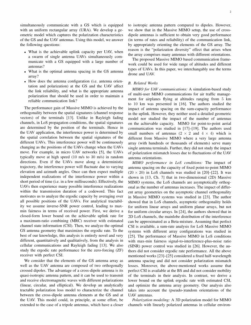
Fig. 1. Illustration of 3D geometric model with a rectangular array at the GS.
ments was developed in [27]. In [28], the authors developed a3D polarization channel model for a 2×2 MIMO configurationin cellular environments with vertical (V) and horizontal (H)polarizations (i.e., V/V, V/H, and ±45 slanted). However,these models cannot be used for UAV communications as thepropagation conditions are different from cellular communi-cations1. A 3D polarization rotation model for both LoS andNLoS conditions was developed in [29]. The authors used asequence of complicated coordinate system transformationsto find the elements of the polarization rotation matrix. Anexperimental study of IEEE 802.11 networks with 3D mobilitywas studied in [7]. It was shown that 5 dB to 15 dB gainsin received signal strength is possible using three linearlypolarized dipole antennas. The authors analyzed the impactof azimuth and elevation angles but they did not analyzethe impact of antenna orientations due to flight dynamics(pitch, yaw, roll). In this work, we develop a simpler method,using rotation matrices for the GS and the UAV antennas toincorporate azimuth, elevation, and flight dynamics.
II. SYSTEM MODEL
A. Geometric Model
We consider an uplink of a Massive MIMO system, withLoS and no multipath. The geometric model of the system is
1The effect of polarization mismatch is not a major problem in cellularcommunications, because irrespective of the type of transmit antenna polar-ization, the large number of multipath components (MPCs) arriving at thereceive antenna will comprise a combination of all polarizations.
shown in Figure 1. We fix an orthonormal coordinate systemwith unit basis vectors x, y, and z and an origin at somepoint O. We refer to this system as a “reference coordinatesystem”. We consider a rectangular antenna array with Mx
and My antennas on x-axis and y-axis, respectively. The totalnumber of antenna elements is denoted by M = MxMy . Thespacing between the antenna elements on x-axis and y-axisis denoted by δx and δy , respectively. The array elements aredescribed by index l = (q−1)Mx+p, where p ∈ 1, 2, ...,Mxdenotes the index on x-axis and q ∈ 1, 2, ...,My denotes theindex on y-axis. The l-th antenna position P l is denoted by(xl, yl, zl) = ((p− 1)δx, (q − 1)δy, 0).
There are K single-antenna UAVs simultaneously trans-mitting data to the GS in the same time-frequency resource.Let the position Pk of the k-th UAV has the coordinates(xk, yk, zk). The direction vector pk from the origin O towardsthe k-th UAV at position Pk can be expressed as
−−→OPk = pk =
(x y z
)xkykzk
=(x y z
)dk cosφk sin θkdk sinφk sin θkdk cos θk
,
where dk is the radial distance between the GS and the k-thUAV, φk ∈ [0, 2π] is the azimuth angle (i.e. the angle fromthe positive direction of the x-axis towards the positive y-axis,to the vector’s (i.e. pk’s) orthogonal projection onto the x-yplane), and θk ∈ [0, π] is the elevation angle (i.e. the angle
4
0
5
0
2
0
2
4
φk
θk
erro
r (%
)
0.5
1
1.5
2
2.5
3
3.5
(a) Relative error with the second term in (3)
0
5
0
1
2
30
2
4
φk
θk
erro
r (%
)
0
0.5
1
1.5
2
2.5
(b) Relative error without the second term in (3)
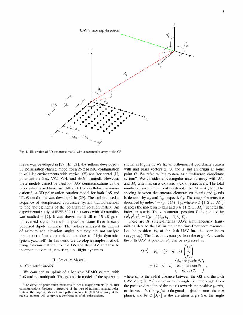
Fig. 2. The approximation error in (3) as a function of the elevation and azimuth angles for Mx = 100,My = 1, dk = 25 m, and δx = 6.25 cm.
from the positive direction of the z-axis towards the directionvector pk).
The distance between the l-th GS antenna and the k-thUAV’s antenna is then given by
dkl =√
(xk − (p− 1)δx)2 + (yk − (q − 1)δy)2 + z2k. (1)
By expanding (1), we get
dkl = dk
[1 +
1
d2k
[(p− 1)2δ2x + (q − 1)2δ2
y] (2)
− 2
dksin θk[(p−1)δx cosφk+(q−1)δy sinφk]
] 12
.
When the distance between the GS antenna and the UAVposition is greater than the aperture size of the array i.e.dk >
√(Mx − 1)2δ2
x + (My − 1)2δ2y , by using the approx-
imation√
1 + t ≈ 1 + t2 , for |t| < 1, the distance in (2) can
be simplified to
dkl ≈dk +1
2dk[(p− 1)2δ2
x + (q − 1)2δ2y]
− sin θk[(p− 1)δx cosφk + (q − 1)δy sinφk].
(3)
Note that in our previous works [1], [2], by assuming dkto be very large when compared to the aperture size, weneglected the second term in (3). However, since the microUAVs typically fly at very low altitudes in the range from30 m to 200 m, the distance dk can be comparable to theaperture size. In this case, the second term in (3) shouldnot be neglected as it will introduce expressive errors in theanalysis. For example, Figure 2 shows the error (in %) withand without including the term 1
2dk
((p− 1)2δ2
x + (q− 1)2δ2y
)for Mx = 100,My = 1, δx = 6.25 cm, and dk = 25 m. Itcan be seen that without the term, the error is significant formost of the elevation and azimuth angles. In contrast, withincluding the term, the error is small for most of the elevationand azimuth angles. Therefore, in this work, we include thesecond term in (3) in our analysis.
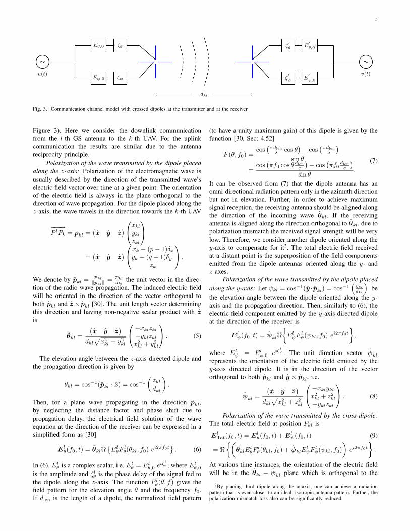
B. Polarization model with single cross-dipole antenna at thetransmitter and the receiver
Let us assume that the l-th GS antenna transmits the signal
u(t) = cos(2πf0t) = <ei2πf0t,
where < denotes the real part. In practice, this signal canbe realized by creating an alternating electrical current ofunit amplitude and frequency f0 in the transmitter’s electricalcircuit. The actual transmission takes place when we applyelectrical current at the transmit antenna. In our model weconsider amplification and phase shifting of the original signalu(t) before applying it to the antenna. The signal’s wavelengthis λ = c/f0, where c ≈ 3× 10⁸ m/s is the speed of light.
If the position and the orientation of the k-th UAV is fixed,the signal at its receiver can be expressed as
v(t) = <√
βkl hkl(f0) e−i2πf0c dkl u(t)
(4)
=√βkl |hkl(f0)| cos
(2πf0
(t− dkl
c
)+ arg(hkl(f0))
),
where βkl =(
λ4πdkl
)2
is the free-space pathloss [30, Sec:2.17.1] and the complex number hkl(f0) represents the com-bined effect of polarization mismatch and antenna gain. In thissubsection we detail the calculation of the factor hkl(f0) forl-th GS antenna the antenna at the UAV.
We fix a translated coordinate system parallel to the refer-ence coordinate system with origin at the l-th GS antenna’sposition P l, i.e. (xl, yl, zl). For the first GS antenna, weget exactly the reference coordinate system. The position Pklof the k-th UAV in the translated coordinate system hascoordinates (xkl, ykl, zkl) = (xk−(p−1)δx, yk−(q−1)δy, zk).Each element of the GS array is composed of two orthogonallycrossed dipoles (one dipole is oriented parallel to the z-axisand the other to the y-axis). As it will be detailed later, thecrossed dipoles are fed with the same signal but with differentmagnitude and phase. The UAV antenna is also composed oftwo crossed dipoles oriented along the y- and z-axes (refer
5
∼
u(t)
Eθ,0 ζθ
dkl
ζ′θ
E′θ,0
Eψ,0 ζψ ζ′ψ E
′ψ,0
∼
v(t)
Fig. 3. Communication channel model with crossed dipoles at the transmitter and at the receiver.
Figure 3). Here we consider the downlink communicationfrom the l-th GS antenna to the k-th UAV. For the uplinkcommunication the results are similar due to the antennareciprocity principle.
Polarization of the wave transmitted by the dipole placedalong the z-axis: Polarization of the electromagnetic wave isusually described by the direction of the transmitted wave’selectric field vector over time at a given point. The orientationof the electric field is always in the plane orthogonal to thedirection of wave propagation. For the dipole placed along thez-axis, the wave travels in the direction towards the k-th UAV
−−−→P lPk = pkl =
(x y z
)xklyklzkl
=(x y z
)xk − (p− 1)δxyk − (q − 1)δy
zk
.
We denote by pkl = pkl‖pkl‖
= pkldkl
the unit vector in the direc-tion of the radio wave propagation. The induced electric fieldwill be oriented in the direction of the vector orthogonal toboth pkl and z× pkl [30]. The unit length vector determiningthis direction and having non-negative scalar product with zis
θkl =
(x y z
)dkl√x2kl + y2
kl
−xklzkl−yklzklx2kl + y2
kl
. (5)
The elevation angle between the z-axis directed dipole andthe propagation direction is given by
θkl = cos−1(pkl · z) = cos−1
(zkldkl
).
Then, for a plane wave propagating in the direction pkl,by neglecting the distance factor and phase shift due topropagation delay, the electrical field solution of the waveequation at the direction of the receiver can be expressed in asimplified form as [30]
Elθ(f0, t) = θkl<
ElθF
lθ(θkl, f0) ei2πf0t
. (6)
In (6), Elθ is a complex scalar, i.e. Elθ = Elθ,0 eiζlθ , where Elθ,0
is the amplitude and ζlθ is the phase delay of the signal fed tothe dipole along the z-axis. The function F lθ(θ, f) gives thefield pattern for the elevation angle θ and the frequency f0.If dlen is the length of a dipole, the normalized field pattern
(to have a unity maximum gain) of this dipole is given by thefunction [30, Sec: 4.52]
F (θ, f0) =cos(πdlen
λ cos θ)− cos
(πdlen
λ
)sin θ
=cos(πf0 cos θ dlen
c
)− cos
(πf0
dlen
c
)sin θ
.
(7)
It can be observed from (7) that the dipole antenna has anomni-directional radiation pattern only in the azimuth directionbut not in elevation. Further, in order to achieve maximumsignal reception, the receiving antenna should be aligned alongthe direction of the incoming wave θkl. If the receivingantenna is aligned along the direction orthogonal to θkl, due topolarization mismatch the received signal strength will be verylow. Therefore, we consider another dipole oriented along they-axis to compensate for it2. The total electric field receivedat a distant point is the superposition of the field componentsemitted from the dipole antennas oriented along the y- andz-axes.
Polarization of the wave transmitted by the dipole placedalong the y-axis: Let ψkl = cos−1(y ·pkl) = cos−1
(ykldkl
)be
the elevation angle between the dipole oriented along the y-axis and the propagation direction. Then, similarly to (6), theelectric field component emitted by the y-axis directed dipoleat the direction of the receiver is
Elψ(f0, t) = ψkl<
ElψF
lψ(ψkl, f0) ei2πf0t
,
where Elψ = Elψ,0 eiζlψ . The unit direction vector ψkl
represents the orientation of the electric field emitted by they-axis directed dipole. It is in the direction of the vectororthogonal to both pkl and y × pkl, i.e.
ψkl =
(x y z
)dkl√x2kl + z2
kl
−xklyklx2kl + z2
kl
−yklzkl
. (8)
Polarization of the wave transmitted by the cross-dipole:The total electric field at position Pkl is
ElTot(f0, t) = El
θ(f0, t) +Elψ(f0, t) (9)
= <(θklE
lθF
lθ(θkl, f0) + ψklE
lψF
lψ(ψkl, f0)
)ei2πf0t
.
At various time instances, the orientation of the electric fieldwill be in the θkl − ψkl plane which is orthogonal to the
2By placing third dipole along the x-axis, one can achieve a radiationpattern that is even closer to an ideal, isotropic antenna pattern. Further, thepolarization mismatch loss also can be significantly reduced.
6
wave travel direction3. Let the vector function El(θkl, ψkl, f0)be defined as
El(θkl, ψkl, f0) =
(ElθF
lθ(θkl, f0)
ElψFlψ(ψkl, f0)
). (10)
The total electric field vector in (9) can be rewritten asEl
Tot(Pkl, f0, t) = <E lei2πf0t
, where E l is the response
vector of the transmit antenna defined as
Ekl =(θkl ψkl
)·El(θkl, ψkl, f0)
= θklElθF
lθ(θkl, f0) + ψklE
lψF
lψ(ψkl, f0).
(11)
The polarization of the electric field can be expressed by theunit vector E l = El
‖El‖ .
Polarization of the receive cross-dipole: Let p′
kl be thepropagation direction unit vector measured from the receiver,i.e. p
′
kl = −pkl. When the transmitted electromagnetic waveis illuminated on the antenna at the receiver side, the inducedfield strength depends on the field patterns of the receivedipoles in the incoming propagation direction. The elevationangles for the receive dipoles oriented along the z- and y-axes are obtained as θ
′kl = cos−1(z · p
′
kl) = cos−1(− zkldkl
)=
π−θkl and ψ′kl = cos−1(y · p
′
kl) = cos−1(− ykldkl
)= π−ψkl,
respectively. Let F′kθ (θ
′kl, f) and F
′kψ (ψ
′kl, f) be the field
patterns of z and y directed receiving dipoles, respectively.The outputs from the dipoles are appropriately amplified andphase shifted in order to match with the polarization of thewave. Let the complex magnitudes of these amplifications beE′kθ = E
′kθ,0 e
iζ′kθ and E
′kψ = E
′kψ,0 e
iζ′kψ . Similarly to (10), we
can define
E′k(θ
′kl, ψ
′kl, f0) =
(E′kθ F
′kθ (θ
′kl, f0)
E′kψ F
′kψ (ψ
′kl, f0)
)(12)
and the response vector of the receive antenna can be writtenas
E′kl = (z y) ·E
′k(θ′kl, ψ
′kl, f0)
= zE′kθ F
′kθ (θ
′kl, f0) + yE
′kψ F
′kψ (ψ
′kl, f0).
(13)
The polarization of the electric field of the receive antenna can
be expressed as E′
k =E′k
‖E′k‖.
Polarization loss factor (PLF): The quantity hkl(f0) in(4) can be obtained by projecting the incident electric fieldvector (Ekl as given in (11)) upon the receiving antennaresponse vector (E
′kl as given in (13)), i.e.
hkl(f0) = Ekl · E′kl = EHklE
′kl
=(El(θkl, ψkl, f0)
)H(θTklψT
kl
)(z y
)E′k(θ
′kl, ψ
′kl, f0)
=(El(θkl, ψkl, f0)
)HTklE
′k(θ′kl, ψ
′kl, f0).
3The polarization (i.e. linear, circular or elliptical) of the resultant waveis determined by the magnitudes and phase difference between the quantitiesElθ and Elψ and the direction of wave propagation. For example, if the twodipoles were fed with equal magnitude (i.e. Elθ,0 = Elψ,0 = 1√
2) and a π
2
phase difference (i.e. ζlθ − ζlψ = π
2) then the polarization along the direction
perpendicular to both dipole axes (the x-axis) would be circular and elliptical(or linear) in other directions (for more details see [30, Sec: 2.12]).
We can calculate the 2× 2 matrix Tkl as
Tkl =
(θT
kl
ψT
kl
)(z y
)=
(θT
klz θT
kly
ψT
klz ψT
kly
)
=1
dkl
√x2kl + y2
kl −yklzkl√x2kl+y
2kl
− yklzkl√x2kl+z
2kl
√x2kl + z2
kl
,
(14)
where the matrix entries denote the polarization mismatchfactors between the orientations of electric field componentsand the dipoles at the UAV. Using this result we obtain that
hkl(f0) =(El(θkl, ψkl, f0)
)HTklE
′k(θ′kl, ψ
′kl, f0)
=1
dkl
(Elθ,0F
lθ(θkl, f0)e−iζ
lθ
Elψ,0Flψ(ψkl, f0)e−iζ
lψ
)T√x2kl + y2
kl −yklzkl√x2kl+y
2kl
− yklzkl√x2kl+z
2kl
√x2kl + z2
kl
×
(E′kθ,0F
′kθ (θ
′kl, f0)eiζ
′kθ
E′kψ,0F
′kψ (ψ
′kl, f0)eiζ
′kψ
)(15)
=
√x2kl + y2
kl
dklElθ,0E
′kθ,0F
lθ(θkl, f0)F
′kθ (θ
′kl, f0)e
i(ζ′kθ −ζ
lθ
)
− yklzkl
dkl√x2kl + y2
kl
Elθ,0E′kψ,0F
lθ(θkl, f0)F
′kψ (ψ
′kl, f0)e
i(ζ′kψ −ζ
lθ
)
− yklzkl
dkl√x2kl+z
2kl
Elψ,0E′kθ,0F
lψ(ψkl, f0)F
′kθ (θ
′kl, f0)e
i(ζ′kθ −ζ
lψ
)
+
√x2kl + z2
kl
dklElψ,0E
′kψ,0F
lψ(ψkl, f0)F
′kψ (ψ
′kl, f0)e
i(ζ′kψ −ζ
lψ
).
The polarization loss factor between the transmitted elec-tromagnetic wave and the receive antennas is given by [30]
PLFkl = |hkl(f0)|2 = |Ekl · E′
kl|2 = |EH
klE′
kl|2
= EH
klE′
kl(E′
kl)H Ekl,
(16)
where (·)H denotes Hermitian transpose. Note that even withfixed orientations of the transmit and receive antennas, ifwe move the receive antenna’s position around the transmitantenna, the PLF can be high for certain elevation and azimuthangles irrespective of the type of polarization of transmit andreceive antennas.
In this subsection we considered the situation when thedipoles at both transmitting and receiving end are aligned withthe y- and z-axes. In the following subsection, we detail thecalculation of hkl(f0) due to the rotation of antennas at thetransmitter and the receiver.
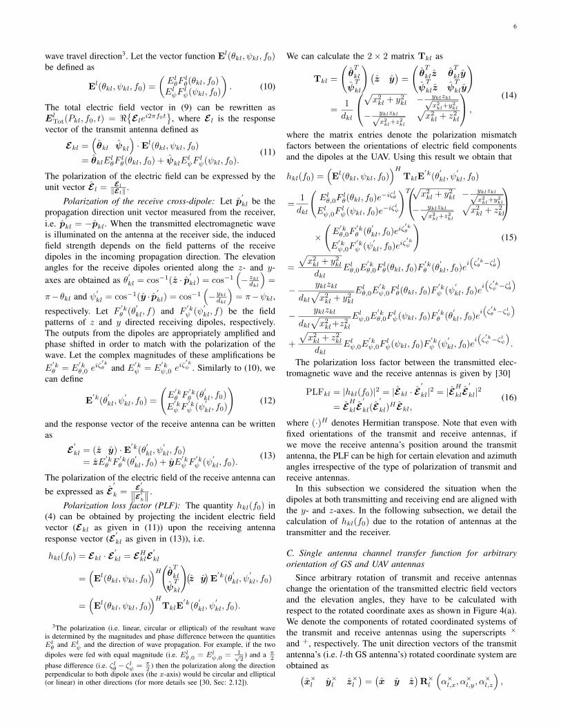
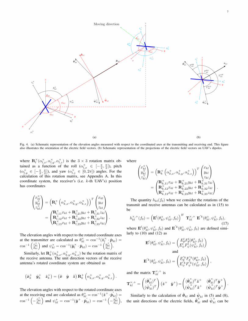
C. Single antenna channel transfer function for arbitraryorientation of GS and UAV antennas
Since arbitrary rotation of transmit and receive antennaschange the orientation of the transmitted electric field vectorsand the elevation angles, they have to be calculated withrespect to the rotated coordinate axes as shown in Figure 4(a).We denote the components of rotated coordinated systems ofthe transmit and receive antennas using the superscripts ×
and +, respectively. The unit direction vectors of the transmitantenna’s (i.e. l-th GS antenna’s) rotated coordinate system areobtained as(
x×l y×l z×l)
=(x y z
)R×l
(α×l,x, α
×l,y, α
×l,z
),
7
x
y
z
x×l
y×l
z×l
ψ×kl
θ×kl
φkl
θkl
ψkl
x
y
z
ψ′kl
θ′kl
x+k
y+k
z+k
ψ+kl
θ+kl
Moving direction
ψ×kl
ψkl
θ×kl
θkl
pkl
(a)
x+k
y+k
z+k
Γψψkl
Γθψkl
Γθθkl
Γψθkl
ψ×kl
θ×kl
rkl
x
y
z
(b)
Fig. 4. (a) Schematic representation of the elevation angles measured with respect to the coordinated axes at the transmitting and receiving end. This figurealso illustrates the orientation of the electric field vectors. (b) Schematic representation of the projections of the electric field vectors on UAV’s dipoles.
where R×l (α×l,x, α×l,y, α
×l,z) is the 3 × 3 rotation matrix ob-
tained as a function of the roll (α×l,x ∈ [−π2 ,π2 ]), pitch
(α×l,y ∈ [−π2 ,π2 ]), and yaw (α×l,z ∈ [0, 2π]) angles. For the
calculation of this rotation matrix, see Appendix A. In thiscoordinate system, the receiver’s (i.e. k-th UAV’s) positionhas coordinates
x×kly×klz×kl
=(R×l
(α×k,x, α
×k,y, α
×k,z
))T xklyklzkl
=
R×l,11xkl + R×l,21ykl + R×l,31zklR×l,12xkl + R×l,22ykl + R×l,32zklR×l,13xkl + R×l,23ykl + R×l,33zkl
.
The elevation angles with respect to the rotated coordinate axesat the transmitter are calculated as θ×kl = cos−1(z×l · pkl) =
cos−1(z×kldkl
)and ψ×kl = cos−1(y×l · pkl) = cos−1
(y×kldkl
).
Similarly, let R+k (α+
k,x, α+k,y, α
+k,z) be the rotation matrix of
the receive antenna. The unit direction vectors of the receiveantenna’s rotated coordinate system are obtained as
(x+k y+
k z+k
)=(x y z
)R+k
(α+k,x, α
+k,y, α
+k,z
).
The elevation angles with respect to the rotated coordinate axesat the receiving end are calculated as θ+
kl = cos−1(z+ · p′
kl) =
cos−1(− z+
kl
dkl
)and ψ+
kl = cos−1(y+ · p′
kl) = cos−1(− y
+kl
dkl
),
wherex+kl
y+kl
z+kl
=(R+k
(α+k,x, α
+k,y, α
+k,z
))T xklyklzkl
=
R+k,11xkl + R+
k,21ykl + R+k,31zkl
R+k,12xkl + R+
k,22ykl + R+k,32zkl
R+k,13xkl + R+
k,23ykl + R+k,33zkl
.
The quantity hkl(f0) when we consider the rotations of thetransmit and receive antennas can be calculated as in (15) tobe
h×,+kl (f0) =(El(θ×kl, ψ
×kl, f0)
)HT×,+kl E
′k(θ+kl, ψ
+kl, f0),
(17)where El(θ×kl, ψ
×kl, f0) and E
′k(θ+kl, ψ
+kl, f0) are defined simi-
larly to (10) and (12) as
El(θ×kl, ψ×kl, f0) =
(ElθF
lθ(θ×kl, f0)
ElψFlψ(ψ×kl, f0)
)and
E′k(θ+
kl, ψ+kl, f0) =
(E′kθ F
′kθ (θ+
kl, f0)
E′kψ F
′kψ (ψ+
kl, f0)
),
and the matrix T×,+kl is
T×,+kl =
((θ×kl)
T
(ψ×kl)
T
)(z+ y+
)=
((θ×kl)
T z+ (θ×kl)
T y+
(ψ×kl)
T z+ (ψ×kl)
T y+
).
Similarly to the calculation of θkl and ψkl in (5) and (8),the unit directions of the electric fields, θ
×kl and ψ
×kl can be
8
calculated in the rotated transmit antenna coordinate systemas
θ×kl =
(x×l y×l z×l
)dkl
√(x×kl)
2 + (y×kl)2
−x×klz×kl
−y×klz×kl
(x×kl)2 + (y×kl)
2
=(x y z
) R×l
(α×l,x, α
×l,y, α
×l,z
)dkl
√(x×kl)
2 + (y×kl)2
−x×klz×kl
−y×klz×kl
(x×kl)2 + (y×kl)
2
and
ψ×kl =
(x×l y×l z×l
)dkl
√(x×kl)
2 + (z×kl)2
−x×kly×kl
(x×kl)2 + (z×kl)
2
−y×klz×kl
=(x y z
) R×l
(α×l,x, α
×l,y, α
×l,z
)dkl
√(x×kl)
2 + (z×kl)2
−x×kly×kl
(x×kl)2 + (z×kl)
2
−y×klz×kl
.Obviously, for the receive antenna dipole directions we have
z+k =
(x+k y+
k z+k
) (0 0 1
)T=(x y z
)R+k
(α+k,x, α
+k,y, α
+k,z
) (0 0 1
)Tand
y+k =
(x+k y+
k z+k
) (0 1 0
)T=(x y z
)R+k
(α+k,x, α
+k,y, α
+k,z
) (0 1 0
)TSince the reference coordinate system is orthonormal, i.e.(x y z
)T (x y z
)= I3, we calculate the matrix T×,+kl
as
T×,+kl =
((θ×kl)
T
(ψ×kl)
T
)(z+ y+
)
=1
dkl
− x×klz×kl√
(x×kl
)2+(y×kl
)2− y×
klz×kl√
(x×kl
)2+(y×kl
)2
√(x×kl)
2 + (y×kl)2
− x×kly×kl√
(x×kl
)2+(z×kl
)2
√(x×kl)
2 + (z×kl)2 − z×
kly×kl√
(x×kl
)2+(z×kl
)2
×R×,+kl
0 00 11 0
, (18)
where R×,+kl is the combined rotation matrix given by
R×,+kl =(R×l
(α×l,x, α
×l,y, α
×l,z
))TR+k
(α+k,x, α
+k,y, α
+k,z
)=
R×,+kl,11 R×,+kl,12 R×,+kl,13
R×,+kl,21 R×,+kl,22 R×,+kl,23
R×,+kl,31 R×,+kl,32 R×,+kl,33
.
Note that the elements of T×,+kl are the projections of theunit electric field vectors components θ
×kl and ψ
×kl on the
receive dipoles unit vectors z+k and y+
k as shown in Figure4(b), i.e.
T×,+kl =
(cos Γθθkl cos Γθψklcos Γψθkl cos Γψψkl
). (19)
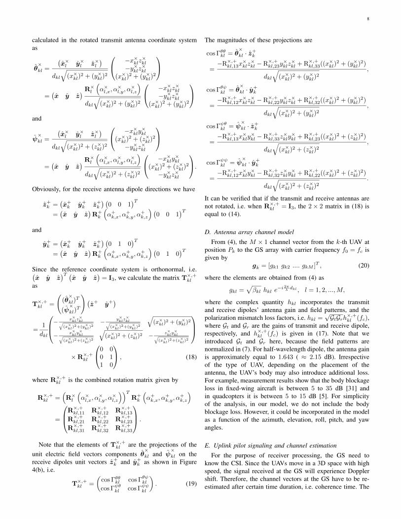
The magnitudes of these projections are
cos Γθθkl = θ×kl · z
+k
=−R×,+kl,13x
×klz×kl − R×,+kl,23y
×klz×kl + R×,+kl,33((x×kl)
2 + (y×kl)2)
dkl
√(x×kl)
2 + (y×kl)2
,
cos Γθψkl = θ×kl · y
+k
=−R×,+kl,12x
×klz×kl − R×,+kl,22y
×klz×kl + R×,+kl,32((x×kl)
2 + (y×kl)2)
dkl
√(x×kl)
2 + (y×kl)2
,
cos Γψθkl = ψ×kl · z
+k
=−R×,+kl,13x
×kly×kl − R×,+kl,33z
×kly×kl + R×,+kl,23((x×kl)
2 + (z×kl)2)
dkl
√(x×kl)
2 + (z×kl)2
,
cos Γψψkl = ψ×kl · y
+k
=−R×,+kl,12x
×kly×kl − R×,+kl,32z
×kly×kl + R×,+kl,22((x×kl)
2 + (z×kl)2)
dkl
√(x×kl)
2 + (z×kl)2
.
It can be verified that if the transmit and receive antennas arenot rotated, i.e. when R×,+kl = I3, the 2× 2 matrix in (18) isequal to (14).
D. Antenna array channel model
From (4), the M × 1 channel vector from the k-th UAV atposition Pk to the GS array with carrier frequency f0 = fc isgiven by
gk = [gk1 gk2 .... gkM ]T , (20)
where the elements are obtained from (4) as
gkl =√βkl hkl e
−i 2πλ dkl , l = 1, 2, ...,M,
where the complex quantity hkl incorporates the transmitand receive dipoles’ antenna gain and field patterns, and thepolarization mismatch loss factors, i.e. hkl =
√GtGrh×,+kl (fc),
where Gt and Gr are the gains of transmit and receive dipole,respectively, and h×,+kl (fc) is given in (17). Note that weintroduced Gt and Gr here, because the field patterns arenormalized in (7). For half-wavelength dipole, the antenna gainis approximately equal to 1.643 ( ≈ 2.15 dB). Irrespectiveof the type of UAV, depending on the placement of theantenna, the UAV’s body may also introduce additional loss.For example, measurement results show that the body blockageloss in fixed-wing aircraft is between 5 to 35 dB [31] andin quadcopters it is between 5 to 15 dB [5]. For simplicityof the analysis, in our model, we do not include the bodyblockage loss. However, it could be incorporated in the modelas a function of the azimuth, elevation, roll, pitch, and yawangles.
E. Uplink pilot signaling and channel estimation
For the purpose of receiver processing, the GS need toknow the CSI. Since the UAVs move in a 3D space with highspeed, the signal received at the GS will experience Dopplershift. Therefore, the channel vectors at the GS have to be re-estimated after certain time duration, i.e. coherence time. The
9
coherence time is defined as a time interval over which the im-pact of Doppler shift on the received signal is insignificant. Weadopt an over-conservative design to re-estimate the channelafter every coherence time Tcoh calculated as follows. Giventhe maximum speed of the UAVs vmax, the coherence time canbe calculated as Tcoh ≈ 1
2fmax, where the Doppler frequency
fmax = vmax
λ . For example, if the maximum speed of UAV is30 m/s, at a carrier frequency of 2.4 GHz, the coherence timeis Tcoh ≈ 2 ms.
As the massive MIMO systems operate in TDD mode,downlink transmission, uplink pilot transmission, and uplinkdata transmission happen within the coherence interval Tlen,i.e. τdl + τul,p + τul,d ≤ Tlen. The parameters τdl, τul,p,and τul,d denote the number of symbols used for downlink,uplink pilot, and uplink data transmission, respectively. Thecoherence interval Tlen is defined as the product of coherencetime and coherence bandwidth. In LoS, since there is nomultipath, the coherence bandwidth is infinite. However, inover-water and mountainous settings, due to a few multipathcomponents, the coherence bandwidth is finite [32]–[34]4.Therefore, we define
Tlen = Tcoh ×Bc =Bc · c
2 · vmax · fc, (21)
where Bc is the coherence bandwidth.During the training phase, K UAVs are assigned K orthog-
onal pilot sequences of length τul,p. Let the M ×K channelmatrix between the GS and the UAVs be G = [g1 g2 ... gK ].The M × τul,p received pilot matrix at the GS is given by
Y p =√ppGΦT +Np,
where pp is transmit power of each pilot symbol, Φ isτul,p × K orthogonal pilot matrix satisfies ΦHΦ = IK andNp is M × τul,p noise matrix with i.i.d CN (0, 1) elements.For notational convenience, we take noise variance to be 1.Therefore, pp can be interpreted as normalized transmit SNR.
In order to obtain reliable channel estimate, the pilot powerhas to be chosen based on the worst-case values of the distanceand effective antenna gain,
pp = ρp
(4πdwc
λ
)21
χwc, (22)
where ρp is the target pilot SNR, dwc is the maximum possibledistance between the GS and UAV, and χwc is the lowestpossible gain over all possible values of azimuth, elevation,and UAV’s rotation angles as discussed in Appendix A, i.e.χwc = min
φ,θ,αx,αy,αz
1M
∑Ml=1 χkl.
4Recent measurements performed in the C-band (5.03–5.091 GHz) showthat the average root-mean-square delay spread is typically very small inover-water (∼ 10 ns), hilly and mountain (∼ 10 ns), suburban and near-urban (10–60 ns) environments (with an average UAV altitude of 600 mand link ranges from 860 m to several kilometers) [32]–[34]. Hence, if thecoherence bandwidth is defined as the bandwidth over which the frequencycorrelation function is above 0.5 [35], depending on the environment thecoherence bandwidth varies between 3 MHz and 20 MHz (300 KHz and2 MHz if the frequency correlation is 0.9). Further, the measured values ofRician K-factors in different environments is greater than 25 dB [32]–[34].Therefore, it is appropriate to consider LoS propagation between the GS andthe UAVs.
The maximum likelihood (ML) estimate of G given Y p is
G =1√ppY pΦ
∗ = G+1√ppW . (23)
Here, W = NpΦ∗ is the estimation error that is uncorrelated
with G. The elements of W are i.i.d zero-mean complexGaussian with unit variance. We use ML as finding theminimum mean square error estimate is nontrivial under theassumed LoS model.
F. Uplink Data Transmission
The M × 1 received signal vector at the GS is given by
y = G(√pu q) + n,
where denotes element wise multiplication; q is the vectorof symbols simultaneously transmitted by the K UAVs, i.e.q = [q1, q2, ..., qK ]T (normalized such that E|qk|2 = 1 forall k ∈ 1, 2, ...,K); pu = [pu1, pu2, ..., puK ]T is the vectorof transmit power of symbols of K UAVs; n is a complexAWGN vector, n ∼ CN (0, IM ).
In order to maintain the same average SNR (ρu) for allUAVs, we consider channel inversion power control, i.e. thepower allocated by the k-th UAV to each data symbol is
puk = min
(ρu
1M
∑Ml=1 βklχkl
, pu
), (24)
where χkl = |hkl|2 and pu is the maximum power availableat the UAV for data symbol. Note that for power control,the UAV needs to know the large scale channel gain (i.e. thedenominator term in (24)). This can be accomplished throughdownlink pilot transmission. Unlike uplink, the downlink pilottransmission requires only one symbol.
We consider that the pilot symbols are transmitted with fixedpower pp according to (22). The value of data power pu iscalculated from the total energy constraint P of each UAV ina coherence interval given by
ppτul,p + puτul,d ≤ P. (25)
Here P is a design parameter selected based on source ofpower supply and flying range of the UAVs. Due to the uplinkpower constraint in (24), the combined effect of free-spacepath loss, polarization mismatch, and directional antenna gainsmay result in signal outage, i.e. the k-th UAV is in outage if
ρu1M
∑Ml=1 βklχkl
> pu. The outage probability is defined as
Pout = P
(ρu
1M
∑Ml=1 βklχkl
> pu
). (26)
When the GS array elements are identically oriented andthe distance between the GS and the UAV location (i.e. dk)is much larger than the aperture size of the GS array, hkl andβkl are approximately the same across the antenna elements,i.e. for all l = 1, 2, ...,M , we have
hkl ≈ hk, βkl ≈ βk, R×,+kl = I3, and
dkl √
(Mx − 1)2δ2x + (My − 1)2δ2
y.(27)
10
Therefore, from (24), we obtain that
puk = min
(ρuβkχk
, pu
). (28)
For analytical tractability, we use (27) and (28) for the ergodicrate analysis in Section III. In Section V, we separately showthe impact of arbitrary orientation of GS array elements onthe link reliability.
III. ACHIEVABLE RATE ANALYSIS
It is known that the linear detectors (MRC and ZF) performfairly well when K M [13]. In this section, we derivethe uplink achievable rate for MRC receiver considering theestimated CSI. For ZF receiver, we analyze the achievable rateconsidering perfect CSI.
A. MRC receiver
By using the MRC detector, the received signal y isseparated into K streams by multiplying it with G
Has follows
r = GHy = G
HG(√pu q) + G
Hn.
Let rk and qk be the k-th elements of the vectors r and q,respectively. Then,
rk =√pukg
Hk gkqk +
∑K
j=1,j 6=k
√puj g
Hk gjqj + gHk n, (29)
where gk is the k-th column of G. In (29), the quantitiesgk and gj will be continuously changing as the positions ofthe UAVs change due to their movement. Even if the locationof the k-th UAV is fixed, it is more likely that any of theother K−1 UAVs will interfere that UAV. Hence, the quantitygHk gj will also be changing as a function of the positions ofthe UAVs i.e. dk, θk, and φk for all k ∈ 1, 2, ...,K. Forexample, in micro UAV networks [5], since the UAVs moveat high speed (10 m/s to 30 m/s) in random directions, onecan expect multiple independent realizations of gHk gj within ashort time duration. For example, consider an ULA with Mx
antennas on the x-axis and My = 1, i.e. M = Mx. If dkand dj are very large when compared to the aperture size ofthe array, after some manipulations, the square of the innerproduct between the channel vectors of the k-th and the j-thUAV can be obtained from (20) and (27) as
|gHk gj |2 =βkβjχkχjM2
×sinc2
(M δx
λ (sin θk cosφk − sin θj cosφj))
sinc2(δxλ (sin θk cosφk − sin θj cosφj)
) .
Here sinc(x) = sin(πx)πx . The fluctuations in |gHk gj |2 are deter-
mined by the following factors: number of antennas, M , an-tenna spacing, δx, velocity, and moving direction of the UAVs.Therefore, by assuming multiple independent realizations ofthe interference power within the codeword transmission time,we compute the ergodic rate by averaging over all possibleUAV positions.
Next we derive closed form expression for achievable rateusing the method from [13] i.e. we assume that the receiverat the GS uses only statistical knowledge of the channel when
performing the detection. The k-th element of r in (29), i.e.rk, can be rewritten in the form√pukrk =EpukgHk gkqk+
(pukg
Hk gk − EpukgHk gk
)qk
+∑K
j=1,j 6=k
√pujpukg
Hk gjqj +
√pukg
Hk n.
(30)By defining the effective additive noise as
a′k =
(pukg
Hk gk − EpukgHk gk
)qk︸ ︷︷ ︸
a1
+∑K
j=1,j 6=k
√pujpukg
Hk gjqj︸ ︷︷ ︸
a2
+√pukg
Hk n︸ ︷︷ ︸
a3
,(31)
the expression in (30) can be written as√pukrk = E
pukg
Hk gk
qk + a′k. (32)
Since EgHk gk is deterministic and qk is independent ofgHk gk, the first two terms of (30) are uncorrelated. Similarly,the last two terms of (30) are uncorrelated with the first term of(30). Hence, the desired signal and the effective additive noisein (32) are uncorrelated. By using the fact that the worst-caseuncorrelated additive noise is independent Gaussian noise ofsame variance [13], the ergodic rate achieved by the k-th UAVcan be lower bounded as
SMRCk ≥ Slb,MRC
k , Λ log2
(1 +|EpukgHk gk|2
var(a′k)
), (33)
where Λ denotes the fraction of symbols used for uplink datatransmission within the coherence length and puk ≤ pu. If thenumber of uplink pilot symbols τul,p = K, then from (21) wecan write
Λ = 1− τdl + τul,p
Tlen= 1− 2 · vmax · fc · (τdl +K)
Bc · c. (34)
Since all three terms in (31) are independent of eachother, the variance of effective noise in (33) is var(a′k) =var(a1) + var(a2) + var(a3). After substituting the expec-tation and variance terms in (33), the lower bound Slb,MRC
k
of the ergodic rate achieved by the k-th UAV is obtained asgiven in (35) (shown on top of next page). For the proof, seeAppendix B.
In (35), it can be observed that the numerator term inside thelogarithm increases proportionally with M . This is an effect ofthe array gain. For example, with 100 antennas and the sameradiated power as in a single-antenna system, the array gainis 20 dB which implies a range extension of 10 times in LoS.The first term in the denominator represents the cumulativeinterference caused by the other K − 1 UAVs. The secondand third terms stem from channel estimation errors and noise,respectively.
Equation (35) can be used to analyze the achievable ratefor any arbitrary distribution and placement of the drones (i.e.distributions of dk, θk, and φk for k ∈ 1, 2, ...,K). Forsome distributions one may have to compute the ergodic ratenumerically as it is difficult to obtain a closed form expression.Next we derive a lower bound on the ergodic rate for the case
11
Slb,MRCk = Λ log2
1 +Mρu
1Mρu
K∑j=1,j 6=k
Epujpuk|gHk gj |2
+(1 +Kρu
)E
1βkχk
(λ
4πdwc
)2χwc
ρuρp+ 1
. (35)
with uniformly distributed UAV locations inside a sphericalshell and the results follow in closed form in this case.
Theorem 3.1: By employing MRC receiver at the GS andusing the ML estimate of the channel matrix, for the inde-pendently and spherically uniformly distributed UAV locationsinside the spherical shell with inner radius
Rmin >√
(Mx − 1)2δ2x + (My − 1)2δ2
y (36)
and outer radius R, the lower bound on the achievable ergodicrate for the k-th UAV is given in (37) (shown on top of nextpage).
Proof: Consider that the UAV positions are independentlyand spherically uniformly distributed within a spherical shellwith inner radius radius Rmin and outer radius R. The distri-bution of the distance dj (for all j ∈ 1, 2, ...,K) is givenby
fdj (r) =3r2
R3 −R3min
, Rmin ≤ r ≤ R. (42)
The distributions of the elevation and azimuth angles are givenby
fθj (θ) =sin θ
2, 0 ≤ θ ≤ π and fφj (φ) =
1
2π, 0 ≤ φ ≤ 2π,
(43)respectively.
By using (42), since χk is independent of the distance (inspherical coordinates χk is only a function of θk and φk), theexpected value of 1
βkχkcan be obtained as
E
1
βkχk
= E
(4πdkλ
)2E
1
χk
= E
1
χk
(4π
λ
)2 ∫ R
Rmin
r2fdk(r) dr (44)
= E
1
χk
(4π
λ
)2 ∫ R
Rmin
r2 3r2
R3 −R3min
dr
=
(4π
λ
)2
κ3(R5 −R5
min)
5(R3 −R3min)
,
where κ = E
1χk
. This expectation has to be calculated
numerically as hkl is a complicated function of rotation angles,field patterns, and polarization mismatch factors. We willdiscuss this in detail in Section V.
The inner product between the channel vectors of k-th andj-th UAVs can be written as
gHk gj =∑M
l=1
√βklβjlhklhjl e
i 2πλ (dkl−djl). (45)
By applying (27), the expression in (45) can be rewritten as
gHk gj =√βkβjhkhj
∑M
l=1ei
2πλ (dkl−djl).
Since |gHk gj |2 = (gHk gj)(gHk gj)
H , we can write
|gHk gj |2 = βkβj |hk|2|hj |2
×
(M∑l=1
ei2πλ (dkl−djl)
)(M∑l′=1
e−i2πλ (dkl′−djl′ )
)
= βkβjχkχj
M∑l=1
M∑l′=1
ei2πλ (dkl−dkl′ ) e−i
2πλ (djl−djl′ ).
The expectation of pujpuk|gHk gj |2 can be written as
Epujpuk|gHk gj |2
= E
(pukβkχk)(pujβjχj)
×M∑l=1
M∑l′=1
ei2πλ (dkl−dkl′ ) e−i
2πλ (djl−djl′ )
.
(46)
Since dkl and djl are independent, by applying (28), theexpectation in (46) can be written as
Epujpuk|gHk gj |2
= ρ2
u
M∑l=1
M∑l′=1
Nkll′ N∗jll′ ,
where
Nkll′ = Eei
2πλ (dkl−dkl′ )
and Njll′ = E
e−i
2πλ (djl−djl′ )
.
Obviously Nkll′ = Njll′ . Therefore,
Epujpuk|gHk gj |2 = ρ2u
∑M
l=1
∑M
l′=1|Nkll′ |2 (47)
= ρ2u
(M +
∑M
l=1
∑M
l′=1,l′ 6=l|Nkll′ |2
).
The distance difference between the l-th and l′-th elements tothe k-th UAV is given by
dkl − dkl′
=1
2dk
[((p− 1)2 − (p′ − 1)2)δ2
x + ((q − 1)2−(q′ − 1)2)δ2y
]− sin θk
[(p− p′)δx cosφk + (q − q′)δy sinφk
].
Since dk, θk, and φk are independent for all k ∈ 1, 2, ...,K,
Nkll′ = E
ei
2πλ (dkl−dkl′ )
(48)
= E
eiπλ
1dk
[((p−1)2−(p′−1)2)δ2x+((q−1)2−(q′−1)2)δ2
y ]
× E
e−i
2πλ sin θk[(p−p′)δx cosφk+(q−q′)δy sinφk]
.
12
Slb,MRCk = Λ log2
1 +Mρu
ρu(K − 1)(1 + ΩM ) + 1 + 1
ρuρp
(1 +Kρu
) 3κχwc(R5−R5min)
5R2(R3−R3min)
, (37)
where
Ω =
M∑l=1
M∑l′=1,l′ 6=l
sinc2
(2
λ
√(p′ − p)2δ2
x + (q′ − q)2δ2y
)×(C2(bll′) + D2(bll′)
), (38)
bll′ =π
λ
(((p− 1)2 − (p′ − 1)2)δ2
x + ((q − 1)2 − (q′ − 1)2)δ2y
), (39)
l = (q − 1)Mx + p, l′ = (q′ − 1)Mx + p′, p, p′ ∈ 1, 2, ...,Mx, q, q′ ∈ 1, 2, ...,My,
C(bll′) =1
2(R3 −R3min)
×
((2R2 − b2ll′
)R cos
(bll′/R
)− bll′R2 sin
(bll′/R
)− b3ll′Si
(bll′/R
)(40)
−(2R2
min − b2ll′)Rmin cos
(b/Rmin
)+ bll′R
2min sin
(bll′/Rmin
)+ b3ll′Si
(bll′/Rmin
)),
D(bll′) =1
2(R3 −R3min)
×
((2R2 − b2ll′
)R sin
(bll′/R
)+ bll′R
2 cos(bll′/R
)+ b3ll′Ci
(b/R
)(41)
−(2R2
min − b2ll′)Rmin sin
(bll′/Rmin
)− bll′R2
min cos(bll′/Rmin
)− b3ll′Ci
(bll′/Rmin
)),
and κ = E
1χk
. Here, Si(x) =
∫ x0
sin tt dt and Ci(x) = −
∫∞x
cos tt dt.
By using (42), the first expectation in (48) can be obtained as
Eeiπλ
1dk
[((p−1)2−(p′−1)2)δ2x+((q−1)2−(q′−1)2)δ2
y ]
= C(bll′) + i D(bll′),
(49)
where bll′ , C(bll′), and D(bll′) are defined in (39), (40), (41),respectively.
By using (43), the second expectation in (48) can beobtained as
Ee−i
2πλ sin θk[(p−p′)δx cosφk+(q−q′)δy sinφk]
= sinc
(2
λ
√(p′ − p)2δ2
x + (q′ − q)2δ2y
).
(50)
For the proofs of (49) and (50), see Appendix C.By substituting (49) and (50) into (48), we obtain that
Nkll′ = (C(bll′) + i D(bll′))
× sinc
(2
λ
√(p′ − p)2δ2
x + (q′ − q)2δ2y
).
(51)
By substituting (51) into (47), we get
Epujpuk|gHk gj |2
= ρ2
u(M + Ω), (52)
where
Ω =
M∑l=1
M∑l′=1,l′ 6=l
sinc2
(2
λ
√(p′ − p)2δ2
x + (q′ − q)2δ2y
)
×(C2(bll′) + D2(bll′)
).
Finally, by using the fact that dwc = R and after substituting(44) and (52) into (35), we get (37).
From the Theorem 3.1, we derive the following result. Whenthe UAVs are located on the surface of the sphere, i.e. whenRmin → R, we obtain that
C(bll′)→1
6R2f ′(R) = cos(bll′/R)
andD(bll′)→
1
6R2g′(R) = sin(bll′/R),
where f ′(x) and g′(x) are the derivatives of
f(x)=(2x2−b2ll′)x cos(bll′x
)−bll′x2 sin
(bll′x
)−b3ll′Si
(bll′x
)and
g(x)=(2x2−b2ll′)x sin(bll′x
)+bll′x
2 cos(bll′x
)+b3ll′Ci
(bll′x
),
respectively.Since C2(bll′)+D2(bll′)→ cos2(bll′/R)+sin2(bll′/R) = 1,
the lower bound becomes as given in (53) (shown on top ofnext page). The quantity Ω1 in (53) depends on the spacingbetween the elements of the GS array. We discuss the impactof antenna spacing on the ergodic rate in Section IV. Notethat since κ = E
1χk
, we have that κχwc < 1.
B. Zero forcing (ZF) receiver
In this section by assuming that perfect CSI is availableat the GS we derive and analyze a lower bound on ergodic
13
Slb,MRCk → Λ log2
(1 +
Mρu
ρu(K − 1)(1 + Ω1
M
)+ 1 + κχwc
ρuρp
(1 +Kρu
)) , Rmin → R, (53)
where Ω1 =M∑l=1
M∑l′=1,l′ 6=l
sinc2
(2λ
√(p′ − p)2δ2
x + (q′ − q)2δ2y
).
capacity with the ZF receiver. By using the ZF detector, thereceived signal y is separated into K streams by multiplyingit with G† =
(GHG
)−1GH as follows
r = G†y.
The output of the ZF detector can be written as
r = G†(G(√pu q) + n
)= (√pu q) +G†n. (54)
Since the first and the second terms in (54) are independent ofeach other, for a given channel matrixG, the K×K covariancematrix of r can be written as
ErrH
∣∣G= E
((√pu q) +G†n
)((√pu q) +G†n
)H= E
(√pu q)(
√pu q)H
+ E
G†nnH(G†)H
= diag(pu1, ..., puK) +G†EnnH(G†)H
= diag(pu1, ..., puK) +G†IM (G†)H
= diag(pu1, ..., puK) + (GHG)−1,
where we used the facts that E
(√pu q)(
√pu q)H
=
diag(pu1, ..., puK), EnnH = IM , and G†(G†)H =(GHG)−1.
The post processing SINR for the k-th UAV is γZFk =
puk[(GHG
)−1]kk
. Since we know that[(GHG
)−1]kk
=
1
det(GHG
)[adj(GHG
)]kk
, we can write
γZFk =
puk det(GHG
)[adj(GHG
)]kk
.
By the convexity of log2
(1 + 1
t
)and Jensen’s inequality, a
lower bound on the achievable uplink rate using ZF receivercan be obtained as
SZFk ≥ Slb,ZF
k = Λ log2
(1 +
(E
1
γZFk
)−1)
(55)
= Λ log2
1 +
(E
[adj(GHG
)]kk
puk det(GHG
))−1,
where puk ≤ pu.The expectation in (55) has to be taken over the distances
dk, the elevation angles θk, and the azimuth angles φk for allk ∈ 1, 2, ...,K. Since it is difficult to find the expectationfor general K UAVs scenario, we analyze the lower bound for
K = 2. In this case, the determinant of GHG can be obtainedas
det(GHG
)= ‖g1‖
2 ‖g2‖2 − (gH1 g2)(gH2 g1)
= M2β1β2χ1χ2
− β1β2χ1χ2
(M +
M∑l=1
M∑l′=1,l′ 6=l
ei2πλ (d1l−d1l′−d2l+d2l′ )
).
We have also[adj(GHG
)]kk
=∥∥g3−k
∥∥2= Mβ3−kχ3−k for
k = 1, 2. Therefore, by applying (28), the expectation in (55)is obtained as
E
[adj(GHG
)]kk
puk det(GHG
) = E
Mβ1β2χ1χ2
ρudet(GHG
) (56)
=1
ρuE
M−(1 +
1
M
M∑l=1
M∑l′=1,l′ 6=l
ei2πλ (d1l−d1l′−d2l+d2l′ )
)−1.
Finally, by substituting (56) into (55), we get the lowerbound as given in (57) (shown on top of next page).
IV. ERGODIC RATE PERFORMANCE WITH OPTIMALANTENNA SPACING
In this section we analyze the ergodic rate performance withoptimal antenna spacing for ULA and URA structures.
A. Optimal antenna spacing
Uniform linear array: For an ULA, i.e. My = 1, sincethe zero crossings of the sinc(u) are at non-zero integer mul-tiples of u, the quantity Ω (as given in (38)) is zero wheneverδx = nλ2 , n = 1, 2, ...,
⌊2Rmin
λ(M−1)
⌋(Here the maximum value
of n is obtained from (36)). Therefore, for an ULA, the optimalantenna spacing for maximizing the ergodic rate is
δ∗x = nλ
2, n = 1, 2, ...,
⌊2Rmin
λ(M − 1)
⌋. (58)
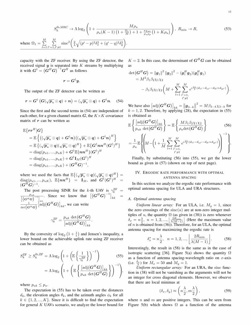
Interestingly, the result in (58) is the same as in the case ofisotropic scattering [36]. Figure 5(a) shows the quantity Ωas a function of antenna spacing-wavelength ratio on x-axis(i.e. δxλ ) for Mx = 50 and My = 1.
Uniform rectangular array: For an URA, the sinc func-tion in (38) will not be vanishing as the arguments will not bean integer for cross diagonal elements. However, we observethat there are local minimas at
(δx, δy) ≈(nλ
2,m
λ
2
), (59)
where n and m are positive integers. This can be seen fromFigure 5(b) which shows Ω as a function of the antenna
14
Slb,ZFk = Λ log2
1 + ρu
EM −
1 +1
M
M∑l=1
M∑l′=1,l′ 6=l
ei2πλ (d1l−d1l′−d2l+d2l′ )
−1−1 , k = 1, 2. (57)
0 0.5 1 1.5 2 2.5 3 3.5 4 4.5 5−50
−40
−30
−20
−10
0
10
Normalized antenna spacing (δx/λ)
Ω (
dB)
(a) Ω (dB) for Mx = 50, My = 1
(b) Ω (dB) for Mx = 5, My = 5
1 2 3 4 5
1
2
3
4
5
δx
λ
δy λ
−15
−10
−5
0
5
(c) Ω (dB) for Mx = 5, My = 5
Fig. 5. Ω as a function of antenna spacing-wavelength ratio for λ = 12.5 cm and R = 500 m.
spacing-wavelength ratio on x-axis ( δxλ ) and y-axis ( δyλ ). Notethat for a given inner radius of the spherical shell Rmin asin (36), the values of n and m are limited by the maximumallowable aperture size of the array, i.e.
(Mx − 1)2n2 + (My − 1)2m2 <4R2
min
λ2.
Furthermore, numerical observations show that Ω is close tozero whenever n ≥ My and m ≥ Mx. For instance, withn = My and m = Mx, we observe that Ω ≈ 0.053. This canbe seen from Figure 5(c) which shows only the values of Ω at(59). Therefore, for an URA, an appropriate choice of antennaspacing for maximizing the ergodic rate could be
(δ∗x, δ∗y) =
(nλ
2,m
λ
2
), n ≥My, m ≥Mx,
(Mx − 1)2n2 + (My − 1)2m2 <4R2
min
λ2.
(60)
B. Achievable rate performance with optimal antenna spacing
MRC receiver: With the optimal antenna spacing as givenin (58) and (60), by employing MRC receiver at the GS, whenRmin → R, from (53) we obtain that
Slb,MRCk (61)
=
Λ log2
(1+ Mρu
ρu(K−1)+1+κχwcρuρp
(1+Kρu)
), for ULA,
Λ log2
(1+ Mρu
ρu(K−1)(
1+ΩURAM
)+1+κχwc
ρuρp(1+Kρu)
), for URA,
where ΩURA =M∑l=1
M∑l′=1,l′ 6=l
sinc2
(√(p′ − p)2n2 + (q′ − q)2m2
),
l = (q − 1)Mx + p, p ∈ 1, 2, ...,Mx, q ∈ 1, 2, ...,My,n ≥My , m ≥Mx, and (Mx−1)2n2+(My−1)2m2 <
4R2min
λ2 .
15
50 100 150 2000
10
20
30
40
50
60
Number of GS antennas (M)
Erg
odic
thro
ughp
ut a
chie
vded
per
UA
V (
Mbp
s)
K = 20K = 50K = 100
(a)
101
102
103
0
1
2
3
4
5
6
Number of UAVs (K)
Sum
thro
ughp
ut (
Gbp
s)
ρu = −10 dB
ρu = 0 dB
ρu = 10 dB
M = 300
M = 100
(b)
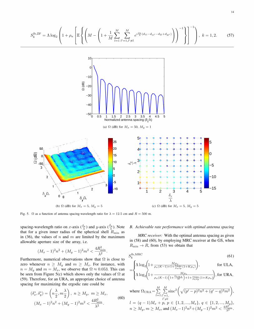
Fig. 6. (a) Ergodic throughput achieved per UAV vs. Number of GS antennas (M ) with the MRC receiver for ρu = 0 dB, ρp = 10 dB, τdl = Tlen8
, B = 20MHz, Bc = 3 MHz, fc = 2.4 GHz, and vmax = 20 m/s. (b) Sum throughput (in Gbps) vs. Number of UAVs for ρp = 10 dB and different values of ρuand M .
For an ULA, the sum rate achieved by the K UAVs is then
SMRCsum,K =
∑K
k=1Slb,MRCk (62)
=ΛK log2
(1 +
Mρuρu(K − 1) + 1 + κχwc
ρuρp(1 +Kρu)
).
It can be observed from (61) that for a given K, the rategrows unbounded with M . If we define ergodic throughput,Q = B ·S bits/sec (where S is the ergodic rate in bits/sec/Hzand B is the system bandwidth in Hz), it can be derived from(61) that when Rmin → R, the minimum number of antennasrequired to support a target data rate of Qtar (bits/s) is
Mreq =
((K − 1) +
1
ρu+κχwc
ρ2uρp
(1 +Kρu)
)(2QtarΛB − 1
).
(63)Figure 6(a) shows the ergodic throughput achieved per UAV
(Q) versus the number of GS antennas (M ) for varying numberof simultaneously communicating UAVs when κχwc = 1,τdl = Tlen
8 , ρu = 0 dB, ρp = 10 dB, B = 20 MHz,Bc = 3 MHz, fc = 2.4 GHz, and vmax = 20 m/s. It canbe seen that, in order to support the data rate of 20 Mbps,for K = 20, 50, and 100 UAVs the number of antennaelements required is approximately equal to 27, 68, and 136,respectively. With the same parameters as in the previous case,Figure 6(b) shows the sum throughput (Qsum = K · B · S)versus the number of UAVs (K) for different values of dataSNR (ρu) and varying number of GS antennas. For a givenρu, the sum throughput increases up to a certain value of Kand decreases with further increase in K. This is because thepre-log term decreases with the number of UAVs due to thefinite number of symbols in a coherence interval.
ZF receiver: With ZF receiver, since it is difficult tocalculate the expectation in (57), we provide the asymp-
totic result. For large M , we observed that the term1M
M∑l=1
M∑l′=1,l′ 6=l
ei2πλ (d1l−d1l′−d2l+d2l′ ) in (57) tends to zero, i.e.
Slb,ZFk
Λ log2 (1 +Mρu)→ 1, k = 1, 2. (64)
Note that when compared to MRC receiver, additional sum-rate performance gains at medium and high SNR regime arepossible with the ZF receiver [13]. This is a topic for futurework.
It is interesting to see from (61) and (64) that only byincreasing the number of antenna elements at the GS, one canincrease the uplink capacity of UAV communication systemwithout increasing the UAV’s transmit power.
Power scaling law: Consider a case with the perfect CSI(i.e. ρp → ∞). If the UAV’s transmit power is scaled downaccording to ρu = εu
M , where εu is fixed, then for large M ,the lower bounds in (61) and (64) (i.e. Slb,MRC
k and Slb,ZFk )
tend to Λ log2(1 + εu). This implies that, with finite K, whenM grows large, each UAV obtains the same rate performanceas in the single UAV case.
V. IMPACT OF POLARIZATION MISMATCH AND ANTENNAPATTERN ON THE LINK RELIABILITY
Since each UAV performs instantaneous power control tomaintain an equal data SNR ρu according to (24), at the GS,the received power on the coherence channel bandwidth Bcremains the same for all drones (i.e. ρu N0 Bc (W), whereN0 is the noise spectral density (i.e. N0 = kB T 10F/10 ≈2× 10⁻²⁰ J, where kB = 1.38× 10⁻²³ J/K, T = 290 K, andthe receiver noise figure F = 7 dB). Therefore, if the distancebetween the GS and the UAV location is much larger than theGS array’s aperture size (i.e. dkl ≈ dk,∀l), for given positions
16
(a)
0 20 40 60 80 100−40
−30
−20
−10
0
10
χ kl (
dB)
GS antenna index (l)
10 log10(
χkl
) 10 log10
(
1
M
∑M
l=1χkl
)
(b)
−10 0 10 200
0.2
0.4
0.6
0.8
1
∑M
l=1 χkl (dB)
CD
F
M=1 M=50
(c)
−30 −20 −10 0 10 200
0.2
0.4
0.6
0.8
1
∑M
l=1 χkl (dB)
CD
F
M=50M=1
(d)
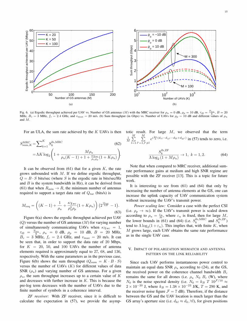
Fig. 7. (a) Effective gain (including antenna gain and polarization mismatch loss) with identically oriented GS array elements for λ = 12 cm, dk =100 m, δx = λ
2m, dlen = λ
2m with Elθ = 1√
2, E′kθ = i√
2and Elψ = E
′kψ = 1√
2. (b) Effective gain with arbitrarily oriented GS array elements for
Mx = 100,My = 1, θk = π3, φk = π. (c) CDF of (
∑Ml=1 χkl) for Mx = 50,My = 1 and Elθ = 1√
2, Elψ = i√
2, E′kθ = 1√
2, E′kθ = −i√
2(circularly
polarized antenna elements; solid lines: identically oriented GS elements, dashed lines: pseudo-randomly oriented GS elements, red lines: isotropic antennapattern, black lines: dipole antenna pattern). (d) CDF of (
∑Ml=1 χkl) for Mx = 50,My = 1 and Elθ = 1, Elψ = 0, E
′kθ = 1, E
′kθ = 0 (linearly polarized
antenna elements).
of GS and k-th UAV, the required transmit power per datasymbol is calculated from (24) as
puk = ρu N0 Bc
(4πdkλ
)21
1M
∑Ml=1 χkl
(W).
Note that the quantity χkl consists of polarization mismatchloss factors, and transmit and receive antenna patterns. Therequired pilot power is obtained using (22) as
pp = ρp N0 Bc
(4πdwc
λ
)21
χwc(W).
Then the instantaneous uplink power (in W) required by thek-th UAV over bandwidth of B Hz is
puk,Tot =B
Bc
(Λ puk +
(K
Tlen
)pp
)= B N0
(4π
λ
)2
(65)
×
Λ ρu d2k
1
1M
M∑l=1
χkl
+
(K
Tlen
)ρp d
2wc
1
χwc
.
In this section, to show the effect of the polarization mis-match loss and antenna patterns we analyze the effective gain∑Ml=1 χkl for the randomly and uniformly distributed UAV po-
17
sitions within a spherical shell with inner radius Rmin = 20 mand outer radius R = 500 m. The uniformly distributed UAVlocations inside a spherical volume are obtained using theprocedure as detailed in [37, p.130]. We consider an ULAwith antenna spacing δx = λ
2 = 6.25 cm (fc = 2.4 GHz). Theroll, pitch, and yaw angles both at the GS and at the UAV areuniformly distributed in the interval [−π2 ,
π2 ], [−π2 ,
π2 ], and
[0, π2 ], respectively.When all GS array elements are identically oriented (i.e.
R×,+kl = I3 and χkl ≈ χk,∀l), with an arbitrarily chosenroll, pitch, and yaw angles, Figure 7(a) shows the effectivegain (χkl) for varying elevation and azimuth angles withElθ = 1√
2, Elψ = i√
2, E
′kθ = E
′kψ = 1√
2. It can be observed
that the gain is very low at certain orientation angles (below−50 dB in some cases). This implies that if all the GS antennaarray elements are identically oriented, most likely the signalwill be lost for certain positions and orientation of the UAV.
For example, consider the following parameters: K = 20,ρu = 10 dB, ρp = 10 dB, τdl = Tlen
8 , B = 20 MHz,Bc = 3 MHz, fc = 2.4 GHz, and vmax = 20 m/s. Ifdk = 400 m, since dwc = R, the total transmit power requiredby the UAV is puk,Tot = 9.2×10⁻³
1M
∑Ml=1 χkl
+ 2.3×10⁻⁵
χwcW. Now the
required uplink power depends on the relative orientation ofthe GS and UAV antenna elements. When all GS elements areidentically oriented, as a result of low gain as shown in Figure7(a), the required uplink power will be very high. For example,if we consider 1
M
∑Ml=1 χkl = −40 dB and χwc = −50 dB,
the required transmit power is puk,Tot ≈ 94 W. Since theUAV’s power supply is limited in practice, the outage proba-bility (as defined in (26)) will be high. This situation can beavoided by arbitrarily orienting the GS array elements.
When all GS array elements are arbitrarily oriented, Fig-ure 7(b) shows the effective gain experienced by an individualantenna element for Mx = 100, My = 1, θk = π
3 , andφk = π. It can be observed that not all elements experiencelow gain. As a result, the nulls as shown in Figure 7(a) canbe canceled out due to polarization diversity. For example,from Figure 7(b), it can be observed that the average gain(i.e. 1
M
∑Ml=1 χkl) is approximately equal to −8 dB.
Figure 7(c) shows the CDF of (∑Ml=1 χkl) with iden-
tical and pseudo-randomly oriented GS elements forMx = 1, 50, My = 1, and Elθ = 1√
2, Elψ = i√
2, E′kθ = 1√
2,
E′kθ = −i√
2(circularly polarized cross-dipoles both at the GS
and at the UAV). The solid and dashed lines denote the gainvalues with identical and pseudo-randomly oriented GS ele-ments, respectively. The black lines represent the gain valueswith an omni-directional antenna pattern (only in the azimuthaldirection) while the red lines represent the gain values powerwith a hypothetical isotropic antenna pattern (i.e. the gain isassumed to be 1 for all θk and φk). Similarly, Figure 7(d)shows the CDF of (
∑Ml=1 χkl) for Mx = 50,My = 1 and
Elθ = 1, Elψ = 0, E′kθ = 1, E
′kθ = 0 (linearly polarized dipoles
both at the GS and at the UAV).From Figures 7(c) and 7(d) we make the following obser-
vations:• By increasing the number of antennas from 1 to 50, the
gain is increased by a factor of 50 (≈ 17 dB).
• Employing linearly polarized antennas either at the GS orUAV results in lower gain. Irrespective of the orientationof the GS array elements, almost always the gain variesbetween −30 and 21 dB.
• Circularly polarized cross-dipoles perform far better thanthe linearly polarized dipoles. Consider a threshold valueof 10 dB gain. When GS elements are identically oriented(solid lines), the probability of experiencing gain below10 dB (This corresponds to 1
M
∑Ml=1 χkl ≈ −7 dB) is
0.045 for circularly polarized cross-dipoles and 0.26 forlinearly polarized dipoles. This is due to the nulls asobserved in Figure 7(a). On the other hand, when the GSelements are pseudo-randomly oriented (dashed lines),the probability is zero and 0.16 for circular polarized andlinearly polarized dipoles, respectively.
• With circularly polarized cross-dipoles, the value ofχwc is around −17 dB for identical orientation and−3.5 dB for arbitrary orientation. This will significantlyreduce the uplink power. For example, if we consider1M
∑Ml=1 χkl = −12 dB and χwc = −20 dB, the required
transmit power is puk,Tot = 0.15 W. This means that,using arbitrarily oriented GS elements, it is possible toachieve 100% coverage with very low uplink transmitpower. As it has been seen earlier, this is not possiblewith identically oriented array elements.
• Since the cross-dipole provides quasi-isotropic gain pat-tern, the gain difference with the isotropic antenna patternis only around 3 dB. By adding third dipole, the differ-ence in gain can be further reduced.
The above results clearly suggest that by using simple cross-dipole antenna elements with circular polarization both at theGS (with arbitrary orientation) and at the UAV one can achievethe link reliability requirements of the UAV networks.
VI. SURVEILLANCE USE CASE
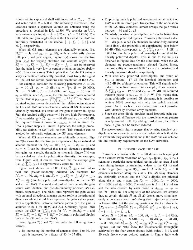
Consider a scenario with K = 20 drones each equippedwith a camera (with resolution of rpy×rpx [pixel], rpy > rpx)scanning a particular geographical region with an area A andtransmitting images or streaming videos to the GS locatedat the origin (see Figure 8(a)). An ULA with Mx = 100elements is located along the x-axis. The GS array elementsare arbitrarily oriented and the UAV’s dipoles are orientedalong the x- and z-axes. Let X1 = −1000, X2 = 2000,Y1 = 2000 and Y2 = 6000. The total area is A = 3 km ×4 kmand the area covered by each drone is Adrone = A
K =600 m ×1000 m. For simplicity of the analysis, we assumethat, at certain altitude H m, all 20 drones move simultane-ously at constant speed v m/s along their trajectory as shownin Figure 8(b). Let the starting position of the k-th drone be(X1 + (i− 1) (X2−X1)
5 , Y1 + j (Y2−Y1)4 , H
), k = 5(j−1)+ i,
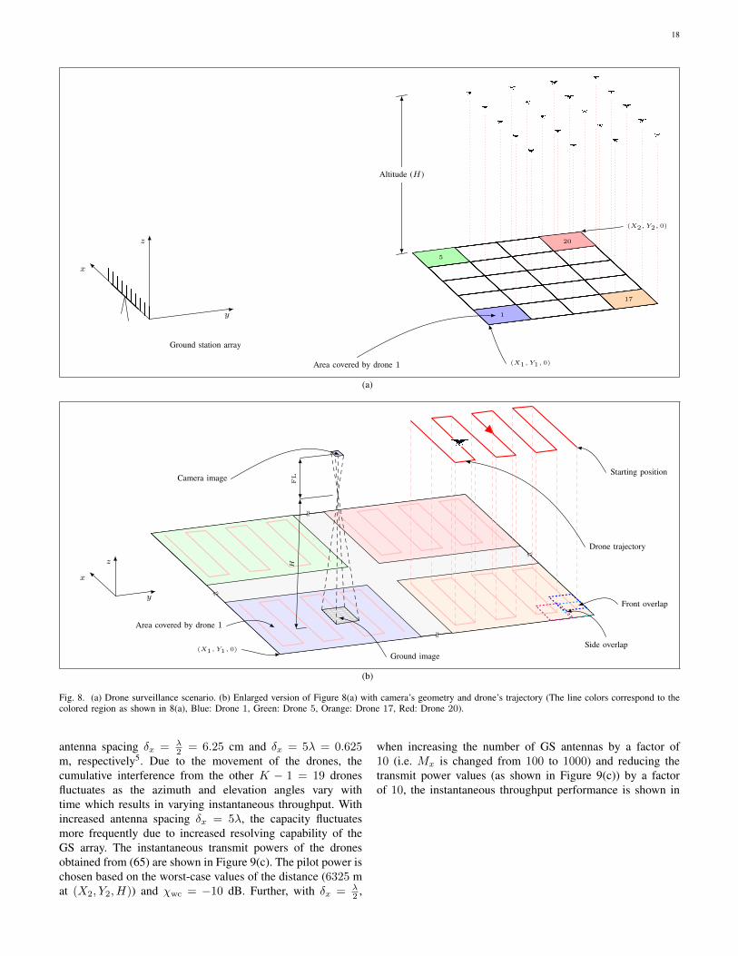
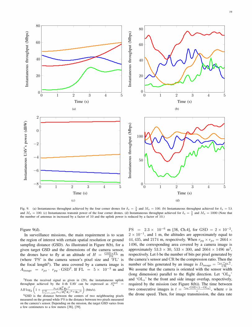
i = 1, ..., 5, j = 1, ..., 4.When H = 100 m, Mx = 100, My = 1, fc = 2.4 GHz,
B = 20 MHz, Bc = 3 MHz, ρu = 10 dB, ρp = 20 dB,v = 30 m/s, and Elθ = i√
2, Elψ = i√
2, E
′kθ = i√
2, E
′kθ = i√
2,
Figures 9(a) and 9(b) show the instantaneous throughputachieved by the four corner drones (with index 1, 5, 17, and20 each drone covers colored regions in Figure 8(a)) with
18
Ground station array
z
x
y 1
5
17
20
Altitude (H)
(X1, Y1, 0)
(X2, Y2, 0)
Area covered by drone 1
(a)
≈
≈
≈
≈
(X1, Y1, 0)
Starting position
Drone trajectory
Side overlap
Front overlap
HF
L
Ground image
Camera image
Area covered by drone 1
z
x
y
(b)
Fig. 8. (a) Drone surveillance scenario. (b) Enlarged version of Figure 8(a) with camera’s geometry and drone’s trajectory (The line colors correspond to thecolored region as shown in 8(a), Blue: Drone 1, Green: Drone 5, Orange: Drone 17, Red: Drone 20).
antenna spacing δx = λ2 = 6.25 cm and δx = 5λ = 0.625
m, respectively5. Due to the movement of the drones, thecumulative interference from the other K − 1 = 19 dronesfluctuates as the azimuth and elevation angles vary withtime which results in varying instantaneous throughput. Withincreased antenna spacing δx = 5λ, the capacity fluctuatesmore frequently due to increased resolving capability of theGS array. The instantaneous transmit powers of the dronesobtained from (65) are shown in Figure 9(c). The pilot power ischosen based on the worst-case values of the distance (6325 mat (X2, Y2, H)) and χwc = −10 dB. Further, with δx = λ
2 ,
when increasing the number of GS antennas by a factor of10 (i.e. Mx is changed from 100 to 1000) and reducing thetransmit power values (as shown in Figure 9(c)) by a factorof 10, the instantaneous throughput performance is shown in
19
0 1 2 3 4 50
20
40
60
80
Time (s)
Inst
anta
neou
sth
roug
hput
(Mbp
s)
(a)
0 1 2 3 4 50
20
40
60
80
Time (s)
Inst
anta
neou
sth
roug
hput
(Mbp
s)
(b)
0 1 2 3 4 5−8
−6
−4
−2
0
2
Time (s)
Inst
anta
neou
sU
AV’s
pow
er(d
BW
)
(c)
0 1 2 3 4 50
50
100
Time (s)
Inst
anta
neou
sth
roug
hput
(Mbp
s)
(d)
Fig. 9. (a) Instantaneous throughput achieved by the four corner drones for δx = λ2
and Mx = 100. (b) Instantaneous throughput achieved for δx = 5λ
and Mx = 100. (c) Instantaneous transmit power of the four corner drones. (d) Instantaneous throughput achieved for δx = λ2
and Mx = 1000 (Note thatthe number of antennas in increased by a factor of 10 and the uplink power is reduced by a factor of 10.)
Figure 9(d).In surveillance missions, the main requirement is to scan
the region of interest with certain spatial resolution or groundsampling distance (GSD). As illustrated in Figure 8(b), for agiven target GSD and the dimensions of the camera sensor,the drones have to fly at an altitude of H = GSD×FL
PS m(where ‘PS’ is the camera sensor’s pixel size and ‘FL’ isthe focal length6). The area covered by a camera image isAimage = rpx · rpy · GSD2. If FL = 5 × 10⁻³ m and
5From the received signal as given in (29), the instantaneous uplinkthroughput achieved by the k-th UAV can be expressed as Sinst
k =
ΛB log2
(1 +
puk|gHk gk|2∑K
j=1,j 6=k puj |gHk
gj |2+|gk|2
)(bits/s).
6GSD is the distance between the centers of two neighbouring pixelsmeasured on the ground while PS is the distance between two pixels measuredon the camera’s sensor. Depending on the mission, the target GSD varies froma few centimeters to a few meters [38], [39].
PS = 2.3 × 10⁻⁶ m [38, Ch.4], for GSD = 2 × 10−2,2 × 10−1, and 1 m, the altitudes are approximately equal to44, 435, and 2174 m, respectively. When rpy × rpx = 2664×1496, the corresponding area covered by a camera image isapproximately 53.3 × 30, 533 × 300, and 2664 × 1496 m2,respectively. Let b be the number of bits per pixel generated bythe camera’s sensor and CR be the compression ratio. Then thenumber of bits generated by an image is Dimage =
rpx·rpy·bCR .
We assume that the camera is oriented with the sensor width(long dimension) parallel to the flight direction. Let ‘OLy’and ‘OLx’ be the front and side image overlap, respectively,required by the mission (see Figure 8(b)). The time betweentwo consecutive images is t =
rpy·GSD·(1−OLy)v , where v is
the drone speed. Then, for image transmission, the data rate
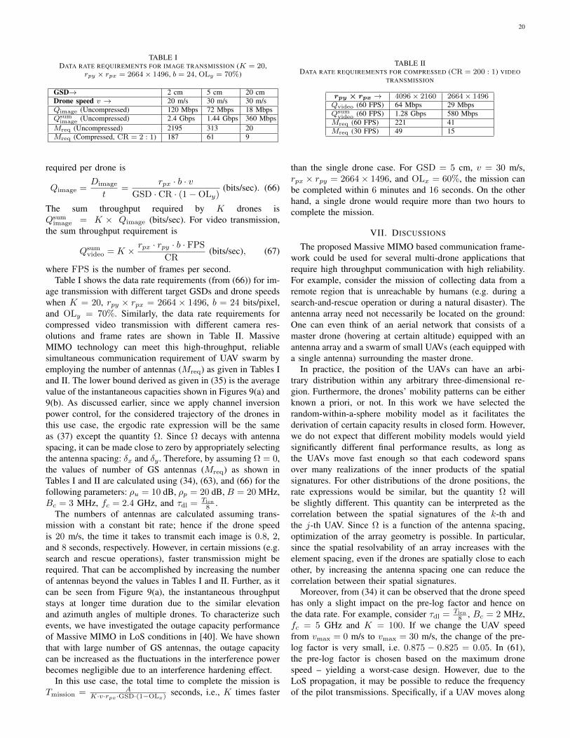
20
TABLE IDATA RATE REQUIREMENTS FOR IMAGE TRANSMISSION (K = 20,
rpy × rpx = 2664× 1496, b = 24, OLy = 70%)
GSD→ 2 cm 5 cm 20 cmDrone speed v → 20 m/s 30 m/s 30 m/sQimage (Uncompressed) 120 Mbps 72 Mbps 18 MbpsQsum
image (Uncompressed) 2.4 Gbps 1.44 Gbps 360 MbpsMreq (Uncompressed) 2195 313 20Mreq (Compressed, CR = 2 : 1) 187 61 9
TABLE IIDATA RATE REQUIREMENTS FOR COMPRESSED (CR = 200 : 1) VIDEO
TRANSMISSION
rpy × rpx → 4096× 2160 2664× 1496Qvideo (60 FPS) 64 Mbps 29 MbpsQsum
video (60 FPS) 1.28 Gbps 580 MbpsMreq (60 FPS) 221 41Mreq (30 FPS) 49 15
required per drone is
Qimage =Dimage
t=
rpx · b · vGSD · CR · (1−OLy)
(bits/sec). (66)
The sum throughput required by K drones isQsum
image = K × Qimage (bits/sec). For video transmission,the sum throughput requirement is
Qsumvideo = K × rpx · rpy · b · FPS
CR(bits/sec), (67)
where FPS is the number of frames per second.Table I shows the data rate requirements (from (66)) for im-
age transmission with different target GSDs and drone speedswhen K = 20, rpy × rpx = 2664 × 1496, b = 24 bits/pixel,and OLy = 70%. Similarly, the data rate requirements forcompressed video transmission with different camera res-olutions and frame rates are shown in Table II. MassiveMIMO technology can meet this high-throughput, reliablesimultaneous communication requirement of UAV swarm byemploying the number of antennas (Mreq) as given in Tables Iand II. The lower bound derived as given in (35) is the averagevalue of the instantaneous capacities shown in Figures 9(a) and9(b). As discussed earlier, since we apply channel inversionpower control, for the considered trajectory of the drones inthis use case, the ergodic rate expression will be the sameas (37) except the quantity Ω. Since Ω decays with antennaspacing, it can be made close to zero by appropriately selectingthe antenna spacing: δx and δy . Therefore, by assuming Ω = 0,the values of number of GS antennas (Mreq) as shown inTables I and II are calculated using (34), (63), and (66) for thefollowing parameters: ρu = 10 dB, ρp = 20 dB, B = 20 MHz,Bc = 3 MHz, fc = 2.4 GHz, and τdl = Tlen
8 .The numbers of antennas are calculated assuming trans-
mission with a constant bit rate; hence if the drone speedis 20 m/s, the time it takes to transmit each image is 0.8, 2,and 8 seconds, respectively. However, in certain missions (e.g.search and rescue operations), faster transmission might berequired. That can be accomplished by increasing the numberof antennas beyond the values in Tables I and II. Further, as itcan be seen from Figure 9(a), the instantaneous throughputstays at longer time duration due to the similar elevationand azimuth angles of multiple drones. To characterize suchevents, we have investigated the outage capacity performanceof Massive MIMO in LoS conditions in [40]. We have shownthat with large number of GS antennas, the outage capacitycan be increased as the fluctuations in the interference powerbecomes negligible due to an interference hardening effect.
In this use case, the total time to complete the mission isTmission = A
K·v·rpx·GSD·(1−OLx) seconds, i.e., K times faster
than the single drone case. For GSD = 5 cm, v = 30 m/s,rpx × rpy = 2664× 1496, and OLx = 60%, the mission canbe completed within 6 minutes and 16 seconds. On the otherhand, a single drone would require more than two hours tocomplete the mission.
VII. DISCUSSIONS
The proposed Massive MIMO based communication frame-work could be used for several multi-drone applications thatrequire high throughput communication with high reliability.For example, consider the mission of collecting data from aremote region that is unreachable by humans (e.g. during asearch-and-rescue operation or during a natural disaster). Theantenna array need not necessarily be located on the ground:One can even think of an aerial network that consists of amaster drone (hovering at certain altitude) equipped with anantenna array and a swarm of small UAVs (each equipped witha single antenna) surrounding the master drone.
In practice, the position of the UAVs can have an arbi-trary distribution within any arbitrary three-dimensional re-gion. Furthermore, the drones’ mobility patterns can be eitherknown a priori, or not. In this work we have selected therandom-within-a-sphere mobility model as it facilitates thederivation of certain capacity results in closed form. However,we do not expect that different mobility models would yieldsignificantly different final performance results, as long asthe UAVs move fast enough so that each codeword spansover many realizations of the inner products of the spatialsignatures. For other distributions of the drone positions, therate expressions would be similar, but the quantity Ω willbe slightly different. This quantity can be interpreted as thecorrelation between the spatial signatures of the k-th andthe j-th UAV. Since Ω is a function of the antenna spacing,optimization of the array geometry is possible. In particular,since the spatial resolvability of an array increases with theelement spacing, even if the drones are spatially close to eachother, by increasing the antenna spacing one can reduce thecorrelation between their spatial signatures.
Moreover, from (34) it can be observed that the drone speedhas only a slight impact on the pre-log factor and hence onthe data rate. For example, consider τdl = Tlen
8 , Bc = 2 MHz,fc = 5 GHz and K = 100. If we change the UAV speedfrom vmax = 0 m/s to vmax = 30 m/s, the change of the pre-log factor is very small, i.e. 0.875 − 0.825 = 0.05. In (61),the pre-log factor is chosen based on the maximum dronespeed – yielding a worst-case design. However, due to theLoS propagation, it may be possible to reduce the frequencyof the pilot transmissions. Specifically, if a UAV moves along
21
a trajectory that is known or can be estimated, its channelresponse may be predicted. This can further boost the payloaddata rate achieved per drone.
Massive MIMO offers both multiplexing gains and a rangeextension due to the array gain. In the surveillance use casedescribed above, the distances between the GS and the fourcorner drones are on the order of several kilometers. Evenwith a single drone, existing wireless standards cannot supportthe required range and throughput, and Massive MIMO maybe the only feasible solution. In particular, Massive MIMOtechnology appears to be much preferable and promising ascompared to multi-hop solutions, which are known to sufferfrom serious drawbacks in terms of reliability and latency [41].
VIII. CONCLUSIONS
Massive MIMO has tremendous potential in the scenarioof communication between a ground station and a swarm ofdrones:• The multiplexing ability of the array offers huge trans-
mission capacity. See Tables I and II for an exam-ple of a drone-swarm surveillance case study, offeringsum throughput of 2.4 Gbps (with 2194 antennas) and1.44 Gbps (with 313 antennas) in 20 MHz bandwidth to20 drones.
• The array gain of M offers a range extension of afactor
√M in line-of-sight. Therefore, the use of Massive
MIMO may reduce the need for multi-hop solutions.Alternatively, the array gain can be used to reduce theUAV’s transmit power by a factor M .
• Maximal-ratio processing with very low complexity andper-antenna distributed processing is sufficient to obtainvery good performance. Additional gains are obtainablethrough zero-forcing as pointed out in Section IV-B.However, a more detailed study of zero-forcing has tobe regarded as future work.
• With (pseudo-) randomly oriented ground station anten-nas, diversity against polarization mismatches is naturallyobtained. This facilitates the use of simple antenna ele-ments, such as cross-dipoles, reducing the concerns ofantenna pattern designs.
• If the drones are uniformly distributed inside of a spher-ical shell, then the optimal antenna spacing is an integermultiple of half a wavelength for a linear array (exactly)and for a rectangular array (approximately).
We hope that the community will reduce our ideas in thispaper to practice in the future and perform field trials.
APPENDIX AAPPENDIX A: 3D ROTATION MODEL
A counterclockwise rotation around the reference coordinateaxes is described by 1) Roll (αx ∈ [−π2 ,
π2 ]): angle of
rotation around the x-axis 2) Pitch (αy ∈ [−π2 ,π2 ]): angle
of rotation around y-axis 3) Yaw (αz ∈ [0, 2π]): angle ofrotation around the z-axis. For example, the transformedunit direction vectors due to a rotation around the x-axisis (x
′y′z′) = (x y z)Rx(αx), where the 3 × 3 matrix
Rx(αx) is given by Rx(αx) =
1 0 00 cosαx − sinαx0 sinαx cosαx
.
Similarly, the rotation matrices around y- and z-axes
are given by Ry(αy) =
cosαy 0 sinαy0 1 0
− sinαy 0 cosαy
and
Rz(αz) =
cosαz − sinαz 0sinαz cosαz 0
0 0 1
, respectively. In prac-
tice, the rotation of the UAVs may take place at around any ofthe three axes irrespective of the current state of the rotation.In that case, the elements of the rotation matrix depend onthe order that the axes are rotated. For example, the rotationmatrix that rotates in the order around z-, y-, and x-axes isobtained by R(αz, αy, αx) = Rx(αx)Ry(αy)Rz(αz).
APPENDIX BAPPENDIX B: PROOF OF EQUATION (35)
1) Calculation of var(a2): The variance of the second termof (31) is
var(a2) =∑K
j=1,j 6=kEpujpuk|gHk gj |2. (68)
Let wk be the k-th column of W . Then, Epujpuk|gHk gj |2in (68) can be obtained as
Epujpuk|gHk gj |2= EpujpukgHk gjgHj gk
= Epujpuk
(gk +
1√ppwk
)Hgjg
Hj
(gk +
1√ppwk
)= E
pujpukg
Hk gjg
Hj gk
+
1√pp
EgHk E
pujpukgjg
Hj E
wk
(69)
+1√pp
EwHk E
pujpukgjg
Hj E
gk
+1
ppEwHk gjg
Hj wk
= E
pujpuk|gHk gj |2
+
1
ppEpujpuk
∥∥gj∥∥2
= Epujpuk|gHk gj |2
+Mρupp
E
1
βkχk
,
where we used the facts that gk and wk are independent,Ewk
= 0, and
∥∥gj∥∥2= Mβjχj .
After substituting (22) and (69) into (68), we get
var(a2) =(K − 1)Mρu
ρpχwc
(λ
4πdwc
)2
E
1
βkχk
+∑Kj=1,j 6=k E
pujpuk|gHk gj |2
.
(70)
2) Calculation of var(a1): The variance of the first termof (31) is
var(a1) = E|pukgHk gk − EpukgHk gk|2
= E
p2uk|g
Hk gk|2
− |EpukgHk gk|2.
(71)
22
From (69), by applying (22) and (28), we get
Ep2uk|g
Hk gk|2 = E
p2uk ‖gk‖
4+1
ppEp2uk ‖gk‖
2 = M2ρ2
u +Mρupp
E
1
βkχk
(72)
and
EpukgHk gk = Epuk
(gk +
1√ppwk
)Hgk
= E
puk ‖gk‖
2+1√pp
EwHk
Epukgk
= E
puk ‖gk‖
2 (73)= Mρu.
After substituting (72) and (73) into (71), we get
var(a1) =Mρuρp
χwc
(λ
4πdwc
)2
E
1
βkχk
. (74)
3) Calculation of var(a3): The variance of the third termof (31) is
var(a3) = EpukgHk nnH gk= E
pukg
Hk nn
Hgk
+1√pp
Epukg
Hk EnnHEwk
+
1√pp
EwHk EnnHEpukgk
+
1
ppEpukw
Hk nn
Hwk
= Mρu +
M
ρpχwc
(λ
4πdwc
)2
E
1
βkχk
.
(75)
After substituting (70), (73), (74), and (75) into (33), we get(35).
APPENDIX CAPPENDIX C: PROOF OF EQUATIONS (49) AND (50)
1) Proof of Equation (49): By letting
bll′ =π
λ
(((p− 1)2− (p′− 1)2)δ2
x + ((q− 1)2− (q′− 1)2)δ2y
),
Equation (49) can be written as
Eeiπλ
1dk
[((p−1)2−(p′−1)2)δ2
x+((q−1)2−(q′−1)2)δ2y
]= E
eibll′dk
(76)
= E cos (bll′/dk)+ iE sin (bll′/dk) .
Here
E
cos(bll′/dk
)=
∫ R
Rmin
cos
(bll′
r
)fdk(r) dr
=
∫ R
Rmin
cos
(bll′
r
)3r2
R3 −R3min
dr
=1
R3 −R3min
(r3 cos
(bll′
r
) ∣∣∣∣RRmin
−∫ R
Rmin
r3d cos
(bll′
r
))=
1
R3 −R3min
(r3 cos
(bll′
r
) ∣∣∣∣RRmin
− bll′∫ R
Rmin
r sin
(bll′
r
)dr
)=
1
R3 −R3min
(r3 cos
(bll′
r
) ∣∣∣∣RRmin
(77)
− bll′
2
(r2 sin
(bll′
r
) ∣∣∣∣RRmin
+ bll′
∫ R
Rmin
cos
(bll′
r
)dr
))
=1
R3 −R3min
(r3 cos
(bll′
r
) ∣∣∣∣RRmin
− bll′
2r2 sin
(bll′
r
)∣∣∣∣RRmin
− b2ll′
2
(r cos
(bll′
r
) ∣∣∣∣RRmin
− bll′∫ R
Rmin
sin(bll′r
)r
dr
))
=1
2(R3 −R3min)
((2r2 − b2ll′)r cos
(bll′
r
) ∣∣∣∣RRmin
− bll′r2 sin
(bll′
r
) ∣∣∣∣RRmin
− b3ll′∫ R
Rmin
sin(bll′r
)r
dr
).
The last integral in (77) can be calculated as
∫ R
Rmin
sin(bll′r
)r
dr = −∫ b
ll′R(bll′/Rmin
) sin(t)
tdt
= −Si(bll′/r
)∣∣∣∣RRmin
(78)
= Si(bll′/R
)− Si
(bll′/Rmin
),
where Si(x) =∫ x
0sin tt dt. By substituting (78) into (77), we
get
E
cos(bll′/dk
)=
1
2(R3 −R3min)
×((
2R2 − b2ll′)R cos
(bll′/R
)− bll′R2 sin
(bll′/R
)+ b3ll′Si
(bll′/R
)−(2R2
min−b2ll′)Rmin cos
(bll′/Rmin
)+ bll′R
2min sin
(bll′/Rmin
)− b3ll′Si
(bll′/Rmin
)).
23
Similarly,
E
sin(bll′/dk
)=
1
2(R3 −R3min)
×((
2R2 − b2ll′)R sin
(bll′/R
)+ bll′R
2 cos(bll′/R
)+ b3ll′Ci
(bll′/R
)−(2R2
min−b2ll′)Rmin sin
(bll′/Rmin
)− bll′R2
min cos(bll′/Rmin
)− b3ll′Ci
(bll′/Rmin
)),
where Ci(x) = −∫∞x
cos tt dt. Now by letting
C(bll′) = E
cos(bll′/dk
)and D(bll′) = E
sin(bll′/dk
),
the expectation in (76) is expressed as given in (49).
2) Proof of Equation (50):
Eei
2πλ ((p−p′)δx sin θk cosφk+(q−q′)δy sin θk sinφk)
=
∫ 2π
0
∫ π
0
ei2πλ ((p−p′)δx sin θ cosφ+(q−q′)δy sin θ sinφ)
× fθk(θ)fφk(φ) dθdφ
=1
4π
∫ 2π
0
∫ π
0
ei2πλ ((p−p′)δx sin θ cosφ+(q−q′)δy sin θ sinφ)sin θ dθdφ.
By letting α1 = (p−p′)δxλ and α2 =
(q−q′)δyλ , the above
integral can be rewritten as
1
4π
∫ 2π
0
∫ π
0
ei2π(α1 sin x cos y+α2 sin x sin y) sinx dxdy.
First we observe that α1 cos y + α2 sin y =√α2
1 + α22
(α1√α2
1+α22
cos y + α2√α2
1+α22
sin y
)and we can
find an angle ξ ∈ [0, 2π), such that cos ξ = α1√α2
1+α22
and
sin ξ = α2√α2
1+α22
. Thus we can simplify the expression as
α1 cos y + α2 sin y =√α2
1 + α22
(cos ξ cos y + sin ξ sin y
)=√
α21 + α2
2 cos(y − ξ), which leads to
1
4π
∫ 2π
0
∫ π
0
ei2π sin x(α1 cos y+α2 sin y) sinx dxdy
=1
4π
∫ 2π
0
∫ π
0
ei2πα sin x cos (y−ξ) sinx dxdy (79)
=1
4π
∫ 2π
0
∫ π
0
ei2πα sin x cos y sinx dxdy,
where α =√α2
1 + α22. By applying the following symmetries
of the trigonometric functions cos y = cos(2π − y),sinx = sin(π − x) and cos y = − cos(π − y) we
consecutively calculate
1
4π
∫ 2π
0
∫ π
0
ei2πα sin x cos y sinx dxdy
=1
2π
∫ π
0
∫ π
0
ei2πα sin x cos y sinx dxdy
=1
π
∫ π
0
∫ π2
0
ei2πα sin x cos y sinx dxdy (80)
=1
π
(∫ π2
0
∫ π2
0
ei2πα sin x cos y sinx dxdy
+
∫ π2
0
∫ π2
0
e−i2πα sin x cos y sinx dxdy
).
By defining the function
h(α) =
∫ π2
0
∫ π2
0
ei2πα sin x cos y sinx dxdy
and using (80), we get
1
4π
∫ 2π
0
∫ π
0
ei2πα sin x cos y sinx dxdy =1
π
(h(α) + h∗(α)
)=
2
π<h(α). (81)
We calculate the Fourier transform of h(α) as
H(f) = Fh(α) =
∫ ∞−∞
h(α)e−i2παfdα
=
∫ ∞−∞
∫ π2
0
∫ π2
0
ei2πα sin x cos y sinx dxdy e−i2παf dα
=
∫ π2
0
∫ π2
0
(∫ ∞−∞
e−i2πα(f−sin x cos y)dα
)sinx dxdy
=
∫ π2
0
∫ π2
0
δ(f − sinx cos y) sinx dxdy (82)
=
∫ π2
0
∫ π2
0δ(f − sinx cos y) sinx dxdy, if f ∈ [0, 1],
0, if f 6∈ [0, 1].
Here we used the facts that sinx cos y ∈ [0, 1] whenx, y ∈
[0, π2
]and that∫A
f(x) δ(g(x))dx =∑
i
f(xi)
|g′(xi)|, (83)
where xi ∈ A ⊆ R are all roots of g(x) (i.e. g(xi) = 0)in the set A. If g(x) has no roots in A, then the integral in(83) is equal to zero. We proceed with the calculation of theinner integral in (82). We observe that in this case we havef ∈ [0, 1], sinx ∈ [0, 1] and cos y ∈ [0, 1]. Using (83) we canconclude that∫ π
2
0
δ(f − sinx cos y) sinx dx
=
sin(arcsin( f
cos y ))
|−cos(arcsin( fcos y )) cos y|
, if f ∈ [0, cos y],
0, if f ∈ (cos y, 1](84)
=
f
cos y√
cos2 y−f2, if y ∈ [0, arccos f ],
0, if y ∈ (arccos f, π2 ].
24
Now we can calculate the double integral in (82) by applyingseveral variable changes. Inserting (84) in (82) we obtain∫ π
2
0
∫ π2
0
δ(f − sinx cos y) sinx dxdy
=
∫ arccos f
0
f
cos y√
cos2 y − f2dy /y = arcsin t/
=
∫ √1−f2
0
f
(1− t2)√
1− t2 − f2dt /t=(p− p′)
√1− f2/
=
∫ 1
0
f
(1− (p− p′)2(1− f2))√
1− (p− p′)2du
/p− p′ = cos t/ (85)
=
∫ π2
0
f
sin2 t+ f2 cos2 tdt
=
∫ π2
0
2f
(f2 + 1) + (f2 − 1) cos 2tdt /t =
π − 2u
4/
=
∫ π2
−π2
f
(f2 + 1) + (f2 − 1) sin(p− p′)du
=f
2farcsin
((f2 + 1) sin(p− p′) + (f2 − 1)
(f2 + 1) + (f2 − 1) sin(p− p′)
)∣∣∣∣π2−π2
=π
2.
Combining (82) and (85) we get
H(f) =π
2rect
(f − 1
2
)=
π2 , if f ∈ [0, 1],
0, if f 6∈ [0, 1],
where the rectangular pulse function is defined as
rect(t) =
1, if t ∈
[− 1
2 ,12
],
0, if t 6∈[− 1
2 ,12
].
The function h(α) can be derived by taking the inverse Fouriertransform H(f) as follows
h(α) = F−1H(f) = π2F−1
rect
(f − 1
2
)=π
2ei2π
12αF−1rect(f) =
π
2eiπαsinc(α).
(86)
Using (79), (81), and (86), the original integral can be obtainedas
1
4π
∫ 2π
0
∫ π
0
ei2π sin x(α1 cos y+α2 sin y) sinx dxdy
=2
π<h(α) =
2
π
π
2<eiπαsinc(α)
= cos(πα) sinc(α) =cos(πα) sin(πα)
πα
=sin(2πα)
2πα= sinc(2α).
(87)
Finally, by substituting α1, α2, and α, we get
Eei
2πλ ((p−p′)δx sin θk cosφk+(q−q′)δy sin θk sinφk)
= sinc
(2λ
√(p− p′)2δ2
x + (q − q′)2δ2y
).
REFERENCES
[1] P. Chandhar, D. Danev, and E. G. Larsson, “Massive MIMO as enablerfor communications with drone swarms,” in Proc. International Confer-ence on Unmanned Aircraft Systems (ICUAS), June 2016, pp. 347–354.
[2] ——, “On ergodic rates and optimal array geometry in line-of-sightMassive MIMO,” in Proc. IEEE SPAWC, July 2016, pp. 1–6.
[3] S. Hayat, E. Yanmaz, and R. Muzaffar, “Survey on unmanned aerialvehicle networks for civil applications: A communications viewpoint,”IEEE Commun. Surveys Tuts., vol. 18, no. 4, pp. 2624–2661, Fourth-Quarter 2016.
[4] L. Gupta, R. Jain, and G. Vaszkun, “Survey of important issues in UAVcommunication networks,” IEEE Commun. Surveys Tuts., vol. 18, no. 2,pp. 1123–1152, Second-Quarter 2016.
[5] M. Asadpour, B. Van den Bergh, D. Giustiniano, K. Hummel, S. Pollin,and B. Plattner, “Micro aerial vehicle networks: An experimental anal-ysis of challenges and opportunities,” IEEE Commun. Mag., vol. 52,no. 7, pp. 141–149, July 2014.
[6] T. Andre, K. Hummel, A. Schoellig, E. Yanmaz, M. Asadpour,C. Bettstetter, P. Grippa, H. Hellwagner, S. Sand, and S. Zhang,“Application-driven design of aerial communication networks,” IEEECommun. Mag., vol. 52, no. 5, pp. 129–137, May 2014.
[7] E. Yanmaz, R. Kuschnig, and C. Bettstetter, “Achieving air-ground com-munications in 802.11 networks with three-dimensional aerial mobility,”in Proc. IEEE INFOCOM, Apr. 2013, pp. 120–124.
[8] M. Asadpour, K. A. Hummel, D. Giustiniano, and S. Draskovic, “Routeor carry: Motion-driven packet forwarding in micro aerial vehiclenetworks,” IEEE Trans. Mobile Comput., vol. 16, no. 3, pp. 843–856,Mar. 2017.
[9] M. Asadpour, D. Giustiniano, K. A. Hummel, S. Heimlicher, andS. Egli, “Now or later?: Delaying data transfer in time-critical aerialcommunication,” in Proc. ACM Conference on Emerging NetworkingExperiments and Technologies CoNEXT, 2013, pp. 127–132.
[10] S. Hayat, E. Yanmaz, and C. Bettstetter, “Experimental analysisof multipoint-to-point UAV communications with IEEE 802.11n and802.11ac,” in Proc. IEEE PIMRC, Aug. 2015, pp. 1991–1996.
[11] Abatti J., Small Power: The Role of Micro and Small UAVs in the Future.Maxwell AFB, AL: Air Command and Staff College, 2005.
[12] P. Olsson, J. Kvarnstrom, P. Doherty, O. Burdakov, and K. Holm-berg, “Generating UAV communication networks for monitoring andsurveillance,” in Proc. International Conference on Control AutomationRobotics Vision (ICARCV), Dec. 2010, pp. 1070–1077.
[13] T. L. Marzetta, E. G. Larsson, H. Yang, and H. Q. Ngo, Fundamentalsof Massive MIMO. Cambridge University Press, 2016.
[14] T. Marzetta, “Noncooperative cellular wireless with unlimited numbersof base station antennas,” IEEE Trans. Wireless Commun., vol. 9, no. 11,pp. 3590–3600, Nov. 2010.
[15] E. G. Larsson, O. Edfors, F. Tufvesson, and T. Marzetta, “MassiveMIMO for next generation wireless systems,” IEEE Commun. Mag.,vol. 52, no. 2, pp. 186–195, Feb. 2014.
[16] J. Rasool, G. Oien, J. Hakegard, and T. Myrvoll, “On multiuser MIMOcapacity benefits in air-to-ground communication for air traffic manage-ment,” in Proc. ISWCS, Sept. 2009, pp. 458–462.
[17] Y. Jiang, A. Tiwari, M. Rachid, and B. Daneshrad, “MIMO for airbornecommunications [industry perspectives],” IEEE Wireless Commun. Mag.,vol. 21, no. 5, pp. 4–6, Oct. 2014.
[18] W. Su, J. D. Matyjas, M. J. Gans, and S. Batalama, “Maximumachievable capacity in airborne MIMO communications with arbitraryalignments of linear transceiver antenna arrays,” IEEE Trans. WirelessCommun., vol. 12, no. 11, pp. 5584–5593, Nov. 2013.
[19] E. T. Michailidis and A. G. Kanatas, “Three-dimensional HAP-MIMOchannels: Modeling and analysis of space-time correlation,” IEEE Trans.Veh. Technol., vol. 59, no. 5, pp. 2232–2242, June 2010.
[20] I. Sarris and A. Nix, “Maximum MIMO capacity in line-of-sight,” inProc. International Conference on Information, Communications andSignal Processing, Dec. 2005, pp. 1236–1240.
[21] F. Bohagen, P. Orten, and G. Oien, “Design of optimal high-rank line-of-sight MIMO channels,” IEEE Trans. Wireless Commun., vol. 6, no. 4,pp. 1420–1425, Apr. 2007.
[22] T. Halsig and B. Lankl, “Array size reduction for high-rank LoS MIMOULAs,” IEEE Microw. Wireless Compon. Lett., vol. 4, no. 6, pp. 649–652, Dec. 2015.
[23] J. Chen, “When does asymptotic orthogonality exist for very largearrays?” in Proc. IEEE GLOBECOM, Dec. 2013, pp. 4146–4150.
[24] Y. Hu, Y. Hong, and J. Evans, “Interference in LoS Massive MIMO iswell approximated by a Beta-mixture,” in Proc. IEEE ICC Workshops,June 2015, pp. 1137–1142.
25
[25] W. Tan, S. Jin, J. Wang, and Y. Huang, “Achievable sum-rate analysis forMassive MIMO systems with different array configurations,” in Proc.IEEE WCNC, Mar. 2015, pp. 316–321.
[26] H. Yang and T. L. Marzetta, “Massive MIMO with max-min powercontrol in line-of-sight propagation environment,” IEEE Transactionson Communications, vol. 65, no. 11, pp. 4685–4693, Nov. 2017.
[27] M. Shafi, M. Zhang, A. Moustakas, P. Smith, A. Molisch, F. Tufvesson,and S. Simon, “Polarized MIMO channels in 3-D: Models, measure-ments and mutual information,” IEEE J. Select. Areas Commun., vol. 24,no. 3, pp. 514–527, Mar. 2006.
[28] M.-T. Dao, V.-A. Nguyen, Y.-T. Im, S.-O. Park, and G. Yoon, “3Dpolarized channel modeling and performance comparison of MIMO an-tenna configurations with different polarizations,” IEEE Trans. AntennasPropag., vol. 59, no. 7, pp. 2672–2682, July 2011.
[29] S. Jaeckel, K. Borner, L. Thiele, and V. Jungnickel, “A geometricpolarization rotation model for the 3-D spatial channel model,” IEEETrans. Antennas Propag., vol. 60, no. 12, pp. 5966–5977, Dec. 2012.
[30] C. A. Balanis, Antenna Theory: Analysis and Design. Wiley-Interscience, 2005.
[31] R. Sun, D. W. Matolak, and W. Rayess, “Air-ground channel character-ization for unmanned aircraft systems–Part IV: Airframe shadowing,”IEEE Trans. Veh. Technol., vol. 66, no. 9, pp. 7643–7652, Sept. 2017.
[32] D. W. Matolak and R. Sun, “Air-ground channel characterization forunmanned aircraft systems–Part I: Methods, measurements, and modelsfor over-water settings,” IEEE Trans. Veh. Technol., vol. 66, no. 1, pp.26–44, Jan. 2017.
[33] R. Sun and D. W. Matolak, “Air-ground channel characterization forunmanned aircraft systems–Part II: Hilly and mountainous settings,”IEEE Trans. Veh. Technol., vol. 66, no. 3, pp. 1913–1925, Mar. 2017.
[34] D. W. Matolak and R. Sun, “Air-ground channel characterization forunmanned aircraft systems–Part III: The suburban and near-urban envi-ronments,” IEEE Trans. Veh. Technol., vol. 66, no. 8, pp. 6607–6618,Aug. 2017.
[35] Rappaport T. S., Wireless Communications Principles and Practice.Prentice Hall Inc., 1996.
[36] P. D. Teal, T. D. Abhayapala, and R. A. Kennedy, “Spatial correlationfor general distributions of scatterers,” IEEE Signal Process. Lett., vol. 9,no. 10, pp. 305–308, Oct. 2002.
[37] D. E. Knuth, The Art of Computer Programming, Volume 2 (3rdEd.): Seminumerical Algorithms. Boston, MA, USA: Addison-WesleyLongman Publishing Co., Inc., 1997.
[38] “Drones and aerial observation: New technologies for property rights,human rights, and global development - A primer,” http://drones.newamerica.org/primer/DronesAndAerialObservation.pdf, [Online], Ac-cessed: December 11, 2017.
[39] T. Rosnell and E. Honkavaara, “Point cloud generation from aerial imagedata acquired by a quadrocopter type micro unmanned aerial vehicle anda digital still camera,” Sensors, vol. 12, no. 1, pp. 453–480, Jan. 2012.
[40] P. Chandhar, D. Danev, and E. G. Larsson, “On the outage capacity inMassive MIMO with line-of-sight,” in Proc. IEEE SPAWC, July 2017,pp. 1–6.
[41] L. R. Pinto, L. Almeida, and A. Rowe, “Demo abstract: Video streamingin multi-hop aerial networks,” in Proc. ACM/IEEE International Con-ference on Information Processing in Sensor Networks, Apr. 2017, pp.283–284.
Prabhu Chandhar received the Ph.D. Degree fromIndian Institute of Technology Kharagpur, West Ben-gal, India. From Nov. 2015 to Oct. 2017, he wasa Postdoctoral Researcher at the Division of Com-munication Systems, Linkoping University (LiU),Linkoping, Sweden. From Aug. 2009 to July 2010,he worked as a Senior Research Fellow at VodafoneIIT KGP Centre of Excellence in Telecommunica-tions (VICET), IIT Kharagpur, India. His researchinterests are within the fields of signal processingand communication theory.
Danyo Danev received his MSc in mathematicsfrom Sofia University in 1996 and his PhD inelectrical engineering from Linkoping University in2001. In 2005 he obtained Docent title in DataTransmission. He is currently Associate Professor atLinkoping University, Sweden. His research interestsare within the fields of coding, information and com-munication theory. He has authored or co-authored 2book chapters, 17 journal papers and more than 30conference papers on these topics. He is currentlyteaching a number of communication engineering
and mathematics courses. Since 2012 he is board member of the IEEE SwedenVT/COM/IT Chapter.
Erik G. Larsson received the Ph.D. degree fromUppsala University, Uppsala, Sweden, in 2002.
He is currently Professor of Communication Sys-tems at Linkoping University (LiU) in Linkoping,Sweden. He was with the Royal Institute of Tech-nology (KTH) in Stockholm, Sweden, the Universityof Florida, USA, the George Washington University,USA, and Ericsson Research, Sweden. In 2015 hewas a Visiting Fellow at Princeton University, USA,for four months. His main professional interests arewithin the areas of wireless communications and
signal processing. He has co-authored some 130 journal papers on thesetopics, he is co-author of the two Cambridge University Press textbooks Space-Time Block Coding for Wireless Communications (2003) and Fundamentalsof Massive MIMO (2016). He is co-inventor on 16 issued and many pendingpatents on wireless technology.
He was Associate Editor for, among others, the IEEE Transactions onCommunications (2010-2014) and the IEEE Transactions on Signal Process-ing (2006-2010). From 2015 to 2016 he served as chair of the IEEE SignalProcessing Society SPCOM technical committee, and in 2017 he is the pastchair of this committee. From 2014 to 2015 he served as chair of the steeringcommittee for the IEEE Wireless Communications Letters. He was the GeneralChair of the Asilomar Conference on Signals, Systems and Computers in2015, and its Technical Chair in 2012. He is a member of the IEEE SignalProcessing Society Awards Board during 2017–2019.
He received the IEEE Signal Processing Magazine Best Column Awardtwice, in 2012 and 2014, the IEEE ComSoc Stephen O. Rice Prize inCommunications Theory in 2015, and the IEEE ComSoc Leonard G. AbrahamPrize in 2017. He is a Fellow of the IEEE.