tutorial – examples - ifat

ADMITADMITTutorial – ExamplesTutorial – ExamplesS Streif A Savchenko P Rumschinski S Borchers R FindeisenS. Streif, A. Savchenko, P. Rumschinski, S. Borchers, R. Findeisen

Otto‐von‐Guericke University Magdeburg, Germanyy g g, yInstitute for Automation EngineeringChair for Systems Theory and Automatic Control

ExamplesA Michaelis Menten kinetics [R mschinski et al 2011 BMC S st Biol ]A Michaelis‐Menten kinetics [Rumschinski et al., 2011, BMC Syst. Biol.]

• step‐by‐step workflow illustration and explanation• parameter estimationp

• outerbounding• bisectioning

B Carnitine Transport mechanism [R mschinski et al 2011 BMC S st Biol ]B Carnitine Transport mechanism [Rumschinski et al., 2011, BMC Syst. Biol.]• data import from table, data uncertainty description • state estimation• uncertainty analysis

C Bio‐Reactor system [Savchenko et al., 2011, IFAC World Congress]• binary variables• detection of discrete state changes (fault detection and diagnosis)• reachability analysis• reachability analysis•Monte‐Carlo

D Adaptation process [Rumschinski et al 2012 in press]D Adaptation process [Rumschinski et al. 2012, in press]• combination of quantative data and qualitative information• combined parameter and state estimation• invalidation of model hypotheses

Refer ADMIT/examples/

Example A: Michaelis‐Menten (Overview)

Task: parameter estimation for Michaelis‐Menten kinetics

Dynamical model Measurements • 20 measurements (sustrate + complex)

i ki i

E S C E ++ P• uncertain (ca 5% relative error)

•mass action kinetics• three unknown parameters

C ti tiContinuous‐time:

A priori knowledge (parameters)

ADMIT/examples/MichaelisMenten/analyzeModel.m

Workflow and Example Highlights

read project fromInitialize project

Set options

ADMITproject()

ADMITsetOptions()

read project from'opt'‐file

choose estimation Set options

Compose

ADMITsetOptions()method

Compose feasibility problem

ADMITcompose()

Estimate ADMITestimate()

/Visualize ADMITplotResults()

ADMITplotBisectioning()plot outerbounding/bisectioning results

Michaelis‐Menten: Structure and syntax of the 'opt' file

Variable section

l• states: real, time‐variant• parameters: real, time‐invariant, of interest

Time set section

• time‐points from sampling

Time‐set section

Constraints sectionConstraints section

•model dynamics, discrete‐time version

• a priori data e.g.parameter bounds

•measurements

Michaelis‐Menten: General Workflow

Read 'opt' file

Set options

• outer bounding • 5 iterations

• bisectioning• bisectioning• 3 recursions

• solverSDP S D Mi• SDP: SeDuMi• LP: cplex, gurobi

Compose problem

Estimate

Visualize

Further scenarios

Summary and Results: Outer‐boundingOuter‐bounding of the parameters p1 p2 p3Outer‐bounding of the parameters p1, p2, p3

Estimateopt = ADMITproject('MichaelisMenten.opt')

Visualize resultsp1 := {real,timeInvariant,ofInterest}2 { l i i f }

Variables optResult = ADMITestimate(optInfo,ops)

ADMITplotResults(optResult,ops)p2 := {real,timeInvariant,ofInterest}p3 := {real,timeInvariant,ofInterest}

Set options

ops =ADMITsetOptions(...'ESTIMATE.outerBounding.use',1,...

Set options

'ESTIMATE.outerBounding.iterations',3)

Compose

optInfo = ADMITcompose(opt,ops) a priori bounds

estimatedbounds

Summary and Results: BisectioningBisection for the parameters p1 p2 p3Bisection for the parameters p1, p2, p3

Estimateopt = ADMITproject('MichaelisMenten.opt')

Visualize resultsp1 := {real,timeInvariant,ofInterest}2 { l i i f }


p2 := {real,timeInvariant,ofInterest}p3 := {real,timeInvariant,ofInterest}

Set options

ADMITplotBisectioning(optResult,ops)

ops = ADMITsetOptions(...'ESTIMATE.bisectioning.use',1,...

Set options

feasible 'ESTIMATE.bisectioning.splitDepth',3)

Composeparameter region

optInfo = ADMITcompose(opt,ops)

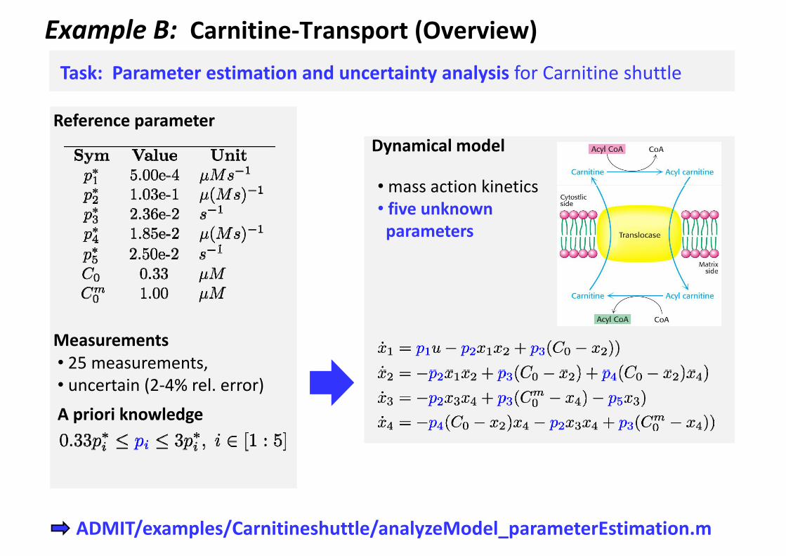
Example B: Carnitine‐Transport (Overview)Task: Parameter estimation and uncertainty analysis for Carnitine shuttle

Reference parameter

•mass action kinetics

Dynamical model Reference parameter

•mass action kinetics• five unknown parameters

Measurements • 25 measurements, ,• uncertain (2‐4% rel. error) A priori knowledge

ADMIT/examples/Carnitineshuttle/analyzeModel_parameterEstimation.m

General Workflow and Example Highlights

Initialize project ADMITproject()

• read measurementsfrom a table

Initialize project ADMITproject()

Import data, ADMITimportData()ADMITprocessData()

• add uncertainty decription

preprocess dataADMITprocessData()ADMITaddData()

Set options ADMITsetOptions()

Compose ADMITcompose()

Estimate ADMITestimate()

Visualize ADMITplotResults()ADMITplotBisectioning()

Carnitine‐Transport: Structure and syntax of the 'opt' file

Variables

• states: x1 x4• states: x1‐x4• parameters: p1‐p5, of interest• constants: C0, C0m, u

Time‐vector

Model dynamicsModel dynamics

• discrete‐time model

A priori data

• a priori bounds on parameters and constants

Carnitine‐Transport: Measurements

•measurements can be included from a table (csv xls )

Measurement data import

measurements can be included from a table (csv, xls,...)• here: import from table (csv), carnitine.dat

optData = ADMITimportData('carnitinedata dat')optData = ADMITimportData( carnitinedata.dat )

Measurement uncertainties

• add uncertainty description if available, here: additive relative error of 4% of all measurements

Measurement uncertainties

optData = ADMITprocessData(optData,{'x1','x2','x3','x4'},[0:5:125],0.04,0.0)

species

relative uncertainty [%]time‐points

y [ ]absolute uncertainty

• data can be plotted and then added to the ADMITprojectADMITplotData(optData,{'x1','x2','x3','x4'})opt = ADMITaddData(opt,optData)

p p j

Carnitine‐Transport: Workflow

Initialize

Import data

• import from table

Set options

• import from table• 4% relative error

Set options

• outerbounding • 5 iterations

Compose

• LP: cplex

Estimate

Visualize

Further scenarios

Carnitine‐Transport: Results (outer‐bounding)O t b di 4% l ti t t i tOuter bounding, 4% relative measurement uncertainty

Estimateopt=ADMITproject('carnitineshuttle_param...

Visualize resultsp1 := {real,timeInvariant,ofInterest}p2 := {real,timeInvariant,ofInterest}


ADMITplotResults(optResult,ops)p3 := {real,timeInvariant,ofInterest}p4 := {real,timeInvariant,ofInterest}p5 := {real,timeInvariant,ofInterest}

A priori data

•

Measurements

• 4% relative error on x1‐x4

ops = ADMITsetOptions(...

Set options

'ESTIMATION.outerBounding.use',1,...'ESTIMATION.outerBounding.iterations',5)

Compose


Carnitine‐Transport: Results (state estimation,outer‐bounding)2% l ti t i t t i t2% relative uncertainty, uncertain parameters

Estimatei bl

opt = ADMITproject('carnitineshuttle_state...

Visualize results

optResult = ADMITestimate(optInfo,ops);

x1 := {real,timeVariant,ofInterest}

Variables

ADMITplotResults(optResult,ops)A priori data

••

Measurements

Set options


ops = ADMITsetOptions(...'ESTIMATE.outerBounding.use',1,...'ESTIMATE.outerBounding.iterations',3,...

p

S .oute ou d g. te at o s ,3,...'YALMIP.solver,'cplex')

Compose


Carnitine‐Transport: Results (state estimation,outer‐bounding)2% l ti t i t t t2% relative uncertainty, exact parameters

Estimatei bl

opt = ADMITproject('carnitineshuttle_state...

Visualize results

optResult = ADMITestimate(optInfo,ops)

x1 := {real,timeVariant,ofInterest}

Variables

ADMITplotResults(optResult,ops)A priori data

•( !)•

Measurements

(exact!)

Set options


pops = ADMITsetOptions(...

'ESTIMATE.outerBounding.use',1,...'ESTIMATE.outerBounding.iterations',3,...

Compose feasibility problem

g'YALMIP.solver,'cplex')


Example C: Two Tank Bioreactor (Overview Fault Diagnosis)T k F lt Di i f t t k bi t

Dynamical model

Task: Fault Diagnosis for two tank bioreactor

• four uncertainparameters

Dynamical model

Reference parameterparameters• two fault scenarios

Measurements (artifical) • uncertain (5% rel. error)

A priori parameter knowledge

• uncertain (±2.5e‐5 abs. error)uncertain (±2.5e 5 abs. error)

ADMIT/examples/TwoTanks/analyzeModel_faultDiagnosis.m

Two Tank System: Workflow (Fault Diagnosis)

•measurements created for 300s with possible occurence of the fault at 150s

Variables

• we consider only one fault at a time• fault scenarios are modelled using binary variables s1, s2:

s1 := {binary,timeInvariant,ofInterest}s1 : {binary,timeInvariant,ofInterest}s2 := {binary,timeInvariant,ofInterest}

• s1: 0 – when valve between tanks is clogged, 1 – when valve functions normally2 0 h t k 1 i l d 1 h t k 1 i l ki

Estimate

• s2: 0 – when tank 1 is sealed, 1 – when tank 1 is leaking

• estimate values of s1, s2 that are consistent with (simulated) measurements data• fault is detected if (s1,s2)=(1,0) is not consistentwith the datawith the data• fault is uniquely diagnosed if only one of the pairs{ (1,0), (0,0), (1,1) } is consistent with the data

t leakagenotconsideredNotes

• here we estimate values of s1, s2 via bisectioningfaultlessclogging

, g

Two Tank System: Result I (Fault Diagnosis)Bisectioning of the fault switches s1 s2Bisectioning of the fault switches s1, s2

Fault Diagnosis

•measurement data (uncertain) provided from the real plant (here simulated)• goal: discard fault scenarios, that cannot represent this measurement data

Faultless system (simulated data) Results I:

t leakagenot considered

faultlessclogging

Two Tank System: Result II (Fault Diagnosis)Bisectioning of the fault switches s1 s2Bisectioning of the fault switches s1, s2

• simulated appearance of the faults (leakage in the tank 1 or clogging of the valve)• unique fault diagnosis: only one considered faulty model is consistent with the data

Leakage at 150s (simulated data) Clogging at 150s (simulated data)

• unique fault diagnosis: only one considered faulty model is consistent with the data

t t

leakage

leakage not

considered notconsidered

faultlessclogging faultlessclogging

Two Tank System: Overview (Reachability Analysis)T k R h bilt A l i f t t k l

Dynamical model

Task: Reachabilty Analysis for two tank example


y

Reference parameterp• two fault scenarios• H1 H2 unknownH1, H2 unknown

Measurements • only (uncertain) initial data (first time step)(first time step)

A priori parameter knowledge • uncertain (±2 5e 5 abs error)• uncertain (±2.5e‐5 abs. error)

ADMIT/examples/TwoTanks/analyzeModel_reachability.m

Two Tank System: Result (Reachability Analysis)Outer bounding of the states for a given time horizonOuter bounding of the states for a given time horizon.

Reachability Analysis

• initial states (uncertain) provided• global bounds assumed unmeasured states• goal: state estimationunder parametric uncertainty

Notes

• user can estimate bounds on the statesat specific time instances (here at everytime instance but the first one)time instance but the first one)• user can fix the values of faulty switchess1, s2 or leave them uncertain• initial global bounds improved by toolboxvia interval arithmetic (thin bars)

Two Tank System: Overview (Monte Carlo)T k M t C l li f t t k l

Dynamical model

Task: Monte Carlo sampling for two tank example


Dynamical model Reference parameter

parameters• two fault scenarios

Measurements • time‐course data• uncertain (5% rel. error)A priori parameter knowledgeA priori parameter knowledge • cL uncertain (±2.5e‐4 abs.)• c2, c12, qp uncertain (±2.5e‐5 abs.)–

ADMIT/examples/TwoTanks/analyzeModel_MonteCarlo.m

Two Tank System: Result (Monte Carlo Sampling)Monte Carlo samplingMonte Carlo sampling

Estimation

• user can create Monte Carlo samples after theproblem is formulated in QP format (optInfo):

[fS,iS] = ADMITMonteCarlo(optInfo,100,ops)

• function produces 100 samples and evaluates in(feasibility)

•measurement data (uncertain) provided

Monte Carlo

• goal: find Monte Carlo samples, that fitthis measurement data

Notes

• outer bounding was performed forouter bounding was performed forthe same problem to compare the results• guaranteed: feasible Monte Carlo samples within the estimated boundswithin the estimated bounds

Example D: Adaptation (Overview)T k bi d t d t t ti ti f d t tiTask: combined parameter and state estimation for adaptation process, using (uncertain) quantitative measurements and qualitative information

Dynamical model Measurements • time‐course data (Aa + Ba)• uncertain (2% relative error)

Qualitative Information (for Ca)

A priori data• parametersp

•Michaelis‐Menten kinetics• five unknown parameters• five unknown parameters

ADMIT/examples/Adaptation/analyzeModel.m

Adaptation (Data)

Measurements Qualitative Information (Ca)

1. after stimulus withdrawal, system adapts to

• time‐course data (Aa + Ba)• uncertain (2% relative error)

prestimulus level within 30s (adaptation)2. Ca never drops below 95% of its initial condition

3 C h i ithi 5 ft3. Ca reaches maximum within 5 s after stimulus is withdrawn

Adaptation (Results)T k bi d t d t t ti ti f d t ti

bl R l (Ill i )

Task: combined parameter and state estimation for adaptation process

p := {binary,timeVariant,ofInterest}p1 := {binary,timeVariant,ofInterest}

Variables Results (Illustration)

p2 := {binary,timeVariant,ofInterest}

Add qualitative information

ADMITconstraint('p <==> &{p1,p2}')AND linked propositions: ADMITconstraint('p <==> |{p1,p2} ')

OR linked propositions:

•models which does not admit the required qualitative behaviorrequired qualitative behavior (adaptation) are invalidated

References (selected)

• P. Rumschinski, S. Borchers, S. Bosio, R. Weismantel, and R. Findeisen. Set‐based dynamicalparameter estimation and model invalidation for biochemical reaction networks. BMC SystemsBiology 4:69 2010Biology, 4:69, 2010. • S. Borchers, S. Bosio, R. Findeisen, U. Haus, P. Rumschinski, and R. Weismantel. Graph problemsarising from parameter identification of discrete dynamical systems. Mathematical Methods ofOperations Research 73(3) 381‐400 2011Operations Research, 73(3), 381 400. 2011.• J. Hasenauer, P. Rumschinski, S. Waldherr, S. Borchers, F. Allgöwer, and R. Findeisen. Guaranteedsteady state bounds for uncertain biochemical processes using infeasibility certificates. J. Proc.Contr., 20(9):1076‐1083, 2010., ( ) ,• S. Borchers, P. Rumschinski, S. Bosio, R. Weismantel, and R. Findeisen. A set‐based framework forcoherent model invalidation and parameter estimation of discrete time nonlinear systems. In 48thIEEE Conf. on Decision and Control, pages 6786 ‐ 6792, Shanghai, China, 2009.p g g• P. Rumschinski , S. Streif . R. Findeisen. Combining qualitative information and semi‐quantitativedata for guaranteed invalidation of biochemical network models. Int. J. Robust Nonlin. Control, 2012. In Press.• S. Streif, S. Waldherr, F. Allgöwer, and R. Findeisen. Systems Analysis of Biological Networks, chapterSteady state sensitivity analysis of biochemical reaction networks: a brief review and new methods,pages 129 ‐148. Methods in Bioengineering. Artech House MIT Press, August 2009.

h• A. Savchenko, P. Rumschinski , R. Findeisen. Fault diagnosis for polynomial hybrid systems. In 18thIFAC World Congress, Milan, Italy, 2011

tutorial – examples - ifat

Documents