1

TUTORIAL #1-2

This tutorial is a minor modification of the model developed in Tutorial 1. This example shows a general

procedure for adjusting the model to current day OIP and saturation levels when historical operations

have included water flooding.

This example shows how to initialize the model at the original conditions and at current conditions and

initiate CO2 injection. Oil production results for this example are much different than for Tutorials 1 or

1-1 due to the difference in the saturations conditions at the start of CO2 injection. Tutorial 1-1 initiated

CO2 injection with oil saturations throughout the reservoir at So = 0.50. The oil was assumed to be

immobile at this saturation. This case initiates CO2 injection with oil saturations in excess of Sorw and

but less than Soi. Oil in excess of Sorw = 0.35 is assumed to be mobile.

The initial OOIP was 2.79 MMSTB. The reservoir is depleted from 1/1/1990 to 1/1/2012 under primary

recovery and water flood operations. The cumulative oil production over the life of the reservoir is 1.08

MMSTB. This suggests an OIP at 1/1/2012 of 1.71 MMSTB. The reservoir pressures are 2500 psia at -

4500 ft ss on 1/1/1990 and 1500 psia at -4500 ft ss on 1/1/2012.

The base case in this tutorial is Tutorial 1. From the Recent projects section in COZView Homepage, load

the project file for Tutorial 1. It is recommended to save the project under a different name using Save

Project As in the Home Page as we will make minor changes to the original project data.

Please note that the PVT properties are the same as in Tutorial 1. Select Saturation Functions from the

Fluid and Saturation properties menu area. Select Rock1 as defined in Tutorial 1.

2

Click Generate to update the relative permeability tables and then Save the rock properties.

Please note that the saturation function used in Tutorial 1 has no capillary pressure. The Water-oil

contact used in the tutorial (-5000 ft ss) is below the reservoir model to assure that the water saturation

is at Swirr (0.35) throughout the reservoir at initial conditions.

The user is required to create a new saturation function to incorporate capillary pressure in the model.

Click Copy to create a copy of the current saturation functions

3

Name the new rock type (R2) and click OK to continue.

��� = ������� � × ∅ × �1 − ��� × � 1���

The Rock Volume, porosity (∅) are constant throughout the simulation. The formation volume factor

(Bo) is a function of reservoir pressure, temperature and fluid composition. The unknown in this

equation is water saturation. This saturation is controlled by the capillary pressure curve. The drainage

curve controls the saturation in the reservoir at the original time (and any point in the reservoir above

the current day WOC) and the imbibition curve controls the saturations in the reservoir at current time

at any point below the implied current WOC. (The original WOC and the implied current WOC will be

different.)

The user should follow the procedure applied in this example for matching current day OIP.

• Calculate capillary pressure value at the midpoint of reservoir

���� = ��� − ����ℎ

����~0.1 × �" #$%�#&' −(�)� �� , �� are water and oil densities, ℎ is the height above (or below) the WOC, WOC is the water-

oil contact at the initialization time.

���� can be positive or negative based on the location of WOC

For this example

Maximum and Minimum Elevation values can be found in the Model Initialization screen.

Original conditions (at 1/1/1900)

Pcow at Zmidpoint ~ 0.1*(-4585.35-(-5000)) = 41.45 psi; WOC is -5000 ft ss

Current condition (at 1/1/2012)

Pcow at Zmidpoint ~ 0.1*(-4585.35-(-4500)) = -8.5 psi; implied WOC is -4500 ft ss

• Generating capillary pressure curves in COZView

Midpoint = -4585.35

TOP = -4537.8

Bottom = -4632.9

4

Set Lambda value to 1.0 (Default) and PEWO to 1 and select Generate. Click on PC-WO to view

Oil-water capillary pressure curves. (PEWO must be greater than zero for a capillary pressure

curve to be generated.)

Note that the scale of PCOW (y-axis) is -60 to 60. The capillary pressure calculated at the midpoint of the

reservoir is 41 and -8 psi respectively for original and current conditions. PCOW at Midpoint at 1/1/1990

should always be much greater than the highest value on the PCOW scale to assure that the Sw = Swirr.

(This PC-WO curve (scale) would suggest a Sw value of approximately 0.37 at the midpoint of the

reservoir which is greater than Swirr.)

Modify the PEWO value to make the scale more appropriate. A higher PEWO value will increase the

scale and a lower PEWO will decrease the scale.

A PEWO value of 0.5 is used in this example. The capillary pressure scale is now set to -30 to 30. The

PCOW at the Midpoint (41 psi) at original conditions is now above the max scale value shown.

5

Go to Model Initialization from the Verify Model menu area. The user must input two Initialization

times and the associated data for 1/1/1990 (original conditions) and 1/1/2012 (current conditions). Use

PVT1 and saturation function R2 for this initialization.

Initialization Date 1/1/1990

Model Type 2 phase

Pressure @Ref 2500

Reference Elevation -4500

Elevation @ WOC -5000 (is below the model)

PSATHCG 800

Initialization Date 1/1/2012

Model Type 2 phase

Pressure @Ref 1500

Reference Elevation -4500

Elevation @ WOC -4500 (is above the model)

PSATHCG 800

6

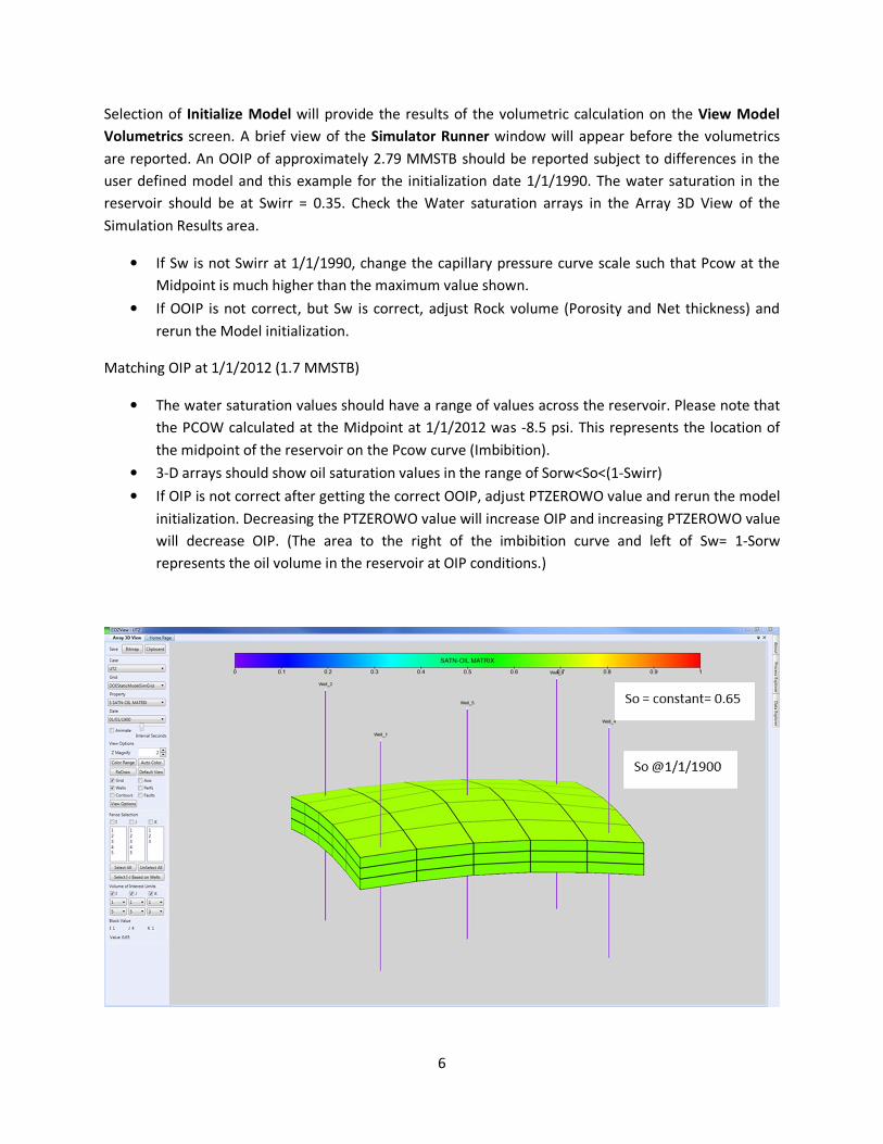
Selection of Initialize Model will provide the results of the volumetric calculation on the View Model

Volumetrics screen. A brief view of the Simulator Runner window will appear before the volumetrics

are reported. An OOIP of approximately 2.79 MMSTB should be reported subject to differences in the

user defined model and this example for the initialization date 1/1/1990. The water saturation in the

reservoir should be at Swirr = 0.35. Check the Water saturation arrays in the Array 3D View of the

Simulation Results area.

• If Sw is not Swirr at 1/1/1990, change the capillary pressure curve scale such that Pcow at the

Midpoint is much higher than the maximum value shown.

• If OOIP is not correct, but Sw is correct, adjust Rock volume (Porosity and Net thickness) and

rerun the Model initialization.

Matching OIP at 1/1/2012 (1.7 MMSTB)

• The water saturation values should have a range of values across the reservoir. Please note that

the PCOW calculated at the Midpoint at 1/1/2012 was -8.5 psi. This represents the location of

the midpoint of the reservoir on the Pcow curve (Imbibition).

• 3-D arrays should show oil saturation values in the range of Sorw<So<(1-Swirr)

• If OIP is not correct after getting the correct OOIP, adjust PTZEROWO value and rerun the model

initialization. Decreasing the PTZEROWO value will increase OIP and increasing PTZEROWO value

will decrease OIP. (The area to the right of the imbibition curve and left of Sw= 1-Sorw

represents the oil volume in the reservoir at OIP conditions.)

7

-30

-20

-10

0

10

20

30

0 0.05 0.1 0.15 0.2 0.25 0.3 0.35 0.4 0.45 0.5 0.55 0.6 0.65 0.7 0.75 0.8 0.85 0.9 0.95 1

PC

OW

Sw

PCOW

PCOWI

Pcow, Sw@1/1/1900 = 41.45

psi, 0.35

Pcow- -8.5 psi; Sw@1/1/2012

= 0.59

8

For this example, a PTZEROWO value of 0.57 is appropriate to match the OIP of 1.71 MMSTB. (It is

suggested that the number of data points be increased from the default of 20 to 40 during this exercise.

This will better display the imbibition curve and the PTZEROWO point.)

Click Done to save the Model Initialization.

9

Select Completions from the Well Data area to view and alter the well completions of the CO2 Injection

well (Well 5) which is perforated only in the bottom layer (Layer 3) in this example.

CO2 injection is initiated in 1/1/2012 as in Tutorial 1.

10

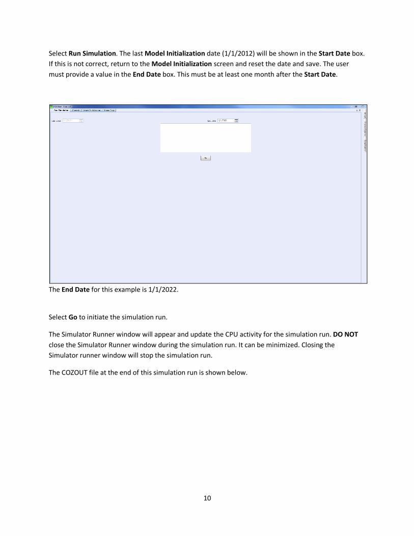
Select Run Simulation. The last Model Initialization date (1/1/2012) will be shown in the Start Date box.

If this is not correct, return to the Model Initialization screen and reset the date and save. The user

must provide a value in the End Date box. This must be at least one month after the Start Date.

The End Date for this example is 1/1/2022.

Select Go to initiate the simulation run.

The Simulator Runner window will appear and update the CPU activity for the simulation run. DO NOT

close the Simulator Runner window during the simulation run. It can be minimized. Closing the

Simulator runner window will stop the simulation run.

The COZOUT file at the end of this simulation run is shown below.

11

In this example, the reservoir is depleted through primary recovery and water flooding from 1/1/1990 to

1/1/2012. The available oil for production at that time is from unswept oil in the rocks. (Much of the

reservoir was not swept to Sorw in this example.) To accomplish a successful prediction run, the user

should make sure that the initial well rates and water cuts of the producers before the start of CO2

injection are consistent with the current day data.

• Check initial oil rates and water cuts to match current data. If the rates are not correct adjust PI

(Productivity Index) of the wells (Process Explorer/Prediction Period/Well Parameters/Well

Productivity Parameters) and/or modify relative permeability curves (Process Explorer/Fluid and

Saturation Properties/Saturation Functions-Advanced Settings).

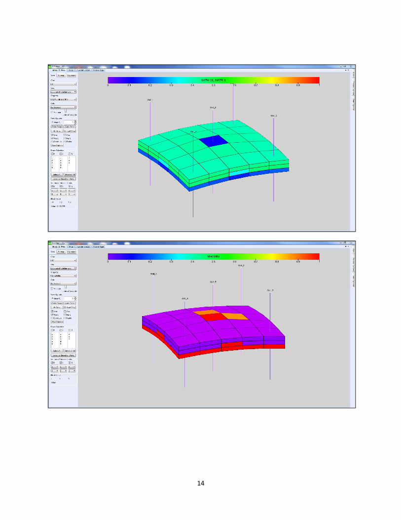
The field cumulative oil produced (due to CO2 injection) by the end of 10 years (1/1/2022) is 0.65

MMSTB and the cumulative CO2 injected is 2.7 BSCF at that time. CO2 Miscibility is achieved around the

injection well and all through Layer 3 as shown in the 3D array at 1/1/2022.

12

13

14