tÍtol: economic development and income inequality. a
TRANSCRIPT

TÍTOL: Economic Development and Income Inequality. A European Case of
Study.
AUTOR: Sergi Quintana Garcia
GRAU: Economia en anglès
TUTOR: Mikel Esnaola Acebes
DATA: 07/06/2019
2
ABSTRACT
This work studies the relationship between economic development and income inequality
in 29 European countries over the period 1995 to 2018. To measure economic
development GDP per capita has been used. To measure income inequality 4 different
proxies have been used: the Gini coefficient and the share of income received by the top
1%, the top 10%, and the bottom 50% income earners. Furthermore, 6 control variables
have been added to the analysis, those variables are: GDP per capita growth (annual %),
inflation measured by consumer prices (annual %), GDP gross domestic savings (% of
GDP), urban population (% of total population) and total general government expenditure
(% of GDP). To test for the effect a total amount of 24 linear mixed effect models have
been produced following a sequential strategy for the variable selection process. The
results obtained shows that there is a negative significant relationship between economic
development and income inequality. Also provides empirical evidences between the link
of the control variables and income inequality. Overall, GDP per capita increases leads to
increases in income inequality, before and after introducing the control variables.

3
CONTENT
1. INTRODUCTION ............................................................................................................... 4
1.1. INEQUALITY AND POVERTY ................................................................................. 4
1.2. WHAT IS ECONOMIC DEVELOPMENT? ................................................................ 6
2. CAUSALITY ....................................................................................................................... 7
3. HISTORICAL EVOLUTION OF INEQUALITY AND THE DIFFERENT
THEORIES REGARDING INCOME AND ITS DISTRIBUTION ....................................... 9
3.1. 18TH AND 19TH CENTURY- THE FIRST THEORIES AND THE CHANGE IN
WORLD DYNAMICS .............................................................................................................. 9
3.2. 20TH CENTURY-THE DATA REVOLUTION .......................................................... 12
3.3. 21ST CENTURY- THE WORLD AFTER KUZNETS................................................ 13
3.4. OVERALL REVISION ............................................................................................... 19
4. DATA ................................................................................................................................. 20
5. METHODOLOGY ............................................................................................................ 22
6. RESULTS AND INTERPRETATION ............................................................................ 23
6.1. GDP PER CAPITA ..................................................................................................... 28
6.2. GDP GROWTH .......................................................................................................... 32
6.3. GDP GROWTH* GDP PER CAPITA ........................................................................ 33
6.4. GOVERNMENT EXPENDITURE ............................................................................ 34
6.5. INFLATION ............................................................................................................... 35
6.6. SAVINGS ................................................................................................................... 36
6.7. URBAN POPULATION ............................................................................................. 37
7. CONCLUSIONS................................................................................................................ 38
8. REFERENCES .................................................................................................................. 41

4
1. INTRODUCTION
Inequalities have existed since the existence of property itself. Some people have always
owned more than others and this has been one of the key elements of the study of social
sciences like sociology or economy. In Oxfam 2018 they warn that the world’s richest
1% are getting 82% of all wealth, and the bottom 50% is getting nothing. Related to
income inequality Lanker and Milanovic 2016 found the so-called elephant curve which
shows how the top income earners of society are the most benefited from economic
growth. Inequality is affected by very different economic and political factors and it is
difficult to know its roots. In Scheidel 2018, Walter Scheidel claims that only very drastic
shocks can reduce inequality, those shocks are war, revolution, and plague.
In the following work, the existence of those inequalities is going to be analyzed together
with the relationship that economic growth has on the global distribution of income. In
the first part of the work, the causality of the relationship between economic development
and income inequality is going to be analyzed. The second part analyzes the evolution of
the different approaches that try to establish a relationship between economic growth and
inequality. After doing a theoretical analysis of the relationship between growth and
inequality, the next section is a quantitative analysis of the relationship between economic
development and income inequality. This is translated into a cross-country analysis of the
relationship between inequality and growth. The analysis will focus on 29 European
countries during the period of 1995 to 2018. To perform this analysis, some proxies will
be chosen as representative for economic development and income inequality.
Furthermore, different control variables will be introduced to enrich the analysis. To test
for this effect different regressions are going to be used. The hypothesis of this work is
that economic development will have a negative impact on income inequality and
probably government intervention will have a positive one.
Before continuing with the work, the concept of inequality and economic growth is going
to be defined to have a proper understanding of the next sections.
1.1.INEQUALITY AND POVERTY
The reader might be confused between inequality and poverty. Both focus mostly on three
dimensions which are income, wealth and consumption. While poverty focuses on the
absolute number of people that falls below a living standard, inequality focuses on the
distribution of income and wealth among individuals of a society. In that sense, inequality
5
answers the question of how well is wealth and income distributed in a society. It is
important to understand the difference between those concepts because later we will see
that economic growth does not affect both in the same way.
Poverty has two main dimensions, the absolute and the relative. According to the Smelser
and Baltes 2001, and to the criteria of the UNESCO , absolute poverty measures poverty
taking into account the money necessary to meet basic needs such as food, clothing, and
shelter while relative poverty analyzes poverty taking a look at the economic position of
an individual compared to the society as a whole: an individual is poor if its economic
status is below the prevailing standards of living of the society. In that sense, relative
poverty is an indicator of inequality. To measure poverty we need to specify a poverty
line and divide the population into poor and non-poor, as explained in Sen 1976. To
analyze poverty, the World Bank created its own poverty line. This poverty line
establishes that the population that falls below a daily income of 2$ are poor, and those
who have less than 1.25$ per day are extremely poor.
Economic inequality has three main dimensions which are income, wealth and
consumption inequality. Income inequality focuses in the differences of income received
by individuals of society whereas wealth inequality focuses on how the wealth of an
economy is distributed among its individuals. Income inequality includes all sources of
inflows of money an individual receives such as wage, interest or returns on capital. On
the other hand, wealth inequality establishes how the ownership of wealth is distributed
in a society. This accounts for how all the assets available in an economy are distributed
among its individuals. The third dimension is consumption, and consist of the different
purchasing power of different individuals of a society. As we can see the three dimensions
are much related among each other: individuals with more wealth, will have a higher
income on the return from capital, and hence, a higher consumption. Nevertheless, it is
important to differentiate among the different types. In this work, the aim is to study
income inequality, so only one of the three economic inequality dimensions is going to
be taken into account in the data analysis.
There are different measures of income inequality, however, the most common measure
is the Lorenz curve. The Lorenz curve is a graphical representation of the percentage
share of income earned by each segment of the population, it has the cumulative share of
income percentage on the vertical axis and the percentage of households by income
distribution on the horizontal axis, see Gaastwirth 1971. In the Lorenz curve, a society

6
without inequality will have a perfect 45-degree line. From the Lorenz curve, the proxies
that will be used in this work as measures of income inequality can be extracted. Those
proxies are the Gini coefficient and the shares of income received by different income
groups (tops 1%, top10% and bottom 50% in this case). The Gini coefficient measures
deviations in the Lorenz curve from the perfect equality line, see Gastwirth 1972, and
establishes a number between 0 and 1, being 0 perfect equality and 1 total inequality.
However, there are some critics of the use of the Gini coefficient as a measure of income
inequality. In Atkinson 1970 the author, referring to the Gini coefficient, concluded that
this conventional method of approach is misleading. The other proxies obtained from the
Lorenz curve are the shares of top income earners. These proxies answer the question of
how much from the total income of a society are the top 1%/10% earners receiving. That
is, the higher the amount received by the top earners, the higher the income inequality of
a society.1
1.2.WHAT IS ECONOMIC DEVELOPMENT?
Development is a multidimensional concept that includes fields such as economic
development, social development, human development, and others. The definition and
purpose of economic development have evolved during the years. At the end of the 60s a
more critic approach towards development appeared and together with the improvements
of data about poverty and inequality did in the 80s and 90s, thanks to the World Bank as
described in Atkinson and Brandolini 2001, employment, poverty, and inequality were
established as the goals of development. A goal achieved with economic growth. In Seers
(1979) the author concludes that the purpose of development should be reducing poverty,
inequality, and unemployment. However, the perception of what development should
achieve have changed and the word has moved towards a poverty approach were the only
goal of development is to reduce poverty. Twenty years later, in Sen (1999) the author
establishes goals different from Seers (1979). He considers development should achieve
a reduction in deprivation. Deprivation is a multidimensional concept that includes things
like hunger, illiteracy, illness, poor health, powerlessness, insecurity, humiliation, and a
lack of access to basic infrastructure. As we can see, what used to include the distribution
of wealth and income as an indicator of development has been forgotten and it just now
1 Visit https://www.chartbookofeconomicinequality.com/economic-
inequality/measures-of-economic-inequality/ for the definition and measures of the
indicators of income inequality.

7
focuses on poverty. This evolution is influenced by the higher elites of society in their
own interest, as described in Stiglitz 2012.
Economic growth is just the mean to achieve economic development, and in the
international community economic growth is measured in terms of income per capita. In
his work Seers (1989) the author wonders why do we confuse economic growth and
development. Here he gives the answer that national income is a very convenient
indicator. We should assume that increases in national income will lead to a reduction of
social and political problems. He also raises the debate that increases in national income
could not only not solve social and political problems, but creates them. To understand
why national income is the indicator of development Stiglitz 2012 proposes that the
richest most influential elite can affect ideas and beliefs and shape it in their favor. For
instance, making us believe that economic growth is beneficial for everybody, and using
it as an indicator of development.
Other indicators have been created in an attempt to measure development in a more
accurate way. This is the case of the Human Development Index, that understands
development as a process of enlarging people’s choices (UNDP 1990). The work of
Prados de la Escosura 2015 found that GDP per capita and human development, measured
by the HDI are uncorrelated over time, which indicates GDP per capita might not be a
good indicator of well-being after all.
Economic well-being should not be measured only by GDP per capita. The way income
and wealth are distributed in a society is almost as important as the total level of wealth
and income the economy is producing. For this reason, to measure development those
variables should be taken into account. The aim of this work is to check for the
relationship between economic growth measured in terms of GDP per capita and income
and wealth inequality, to see whereas improvements in GDP per capita are beneficial or
prejudicial for the distribution of income and wealth of an economy.
2. CAUSALITY
There is a lot of research regarding the relationship between economic growth and
inequality. However, the causality of the relationship between those two variables is not
clear.

8
Most of the authors decide to study the relationship trying to see how inequality affects
economic growth. Since most of the authors are only concerned about the sources of
growth, i.e., how GDP per capita is increased, this has led authors to study the effect of
the initial distribution of wealth and income on economic growth instead of analyzing
how this growth affects the distribution of wealth. Person and Tabellini 1994 concluded
that income inequality is not beneficial for growth because it implies economic policies
that led property rights unprotected. Alesina and Rodrik 1994 also concluded that income
and land inequality are negatively correlated with economic growth. Moreover, in
Cingano 2014 the authors found income inequality has a negative impact on growth, but
it remains unaffected by redistributive policies towards equality. To see for more studies
that have found a negative relationship see Murphy 1989, Sukissayan 2007 or
Tachibanaki 2005.
However, not all the studies concluded the same. In Barro 2000 the author found that
inequality affects differently poor and rich countries. In poor countries inequality retards
growth but in rich countries inequality led to higher levels of growth. Furthermore, there
are authors that have found a positive relationship between the initial level of inequality
and economic growth. Li and Zou 1998 proved both theoretically and empirically that
income inequality is positively associated with economic growth. Forbes 2000 also
concluded that inequality and economic growth are positively correlated. So in
conclusion, the correlation between inequality and growth is unambiguous, with different
studies obtaining different results.
Nevertheless, in this work, the causality is analyzed in the opposite way. The interest of
this work is to analyze the effect of economic growth on inequality. Instead of analyzing
the sources of economic growth in an attempt to maximize it, the aim of this work is to
understand the consequences of this growth. There are authors that have understood the
causality in this direction and there are studies in this field. In Aghion, Caroli and García-
Peñalosa 1999 the authors ask themselves whereas there is a virtuous cycle by which a
reduction in inequality will imply an acceleration of growth and thereby induce further
reductions in inequality or, on the contrary, there is a vicious cycle because growth
increases inequality and calls for a permanent redistribution. As an answer to this
question, there have been a lot of authors that have asked themselves how the increase in
the total level of output affects the shape of the distribution of wealth on an economy. In
the following section, a review of the different literature on this topic is going to be done.
9
3. HISTORICAL EVOLUTION OF INEQUALITY AND THE DIFFERENT
THEORIES REGARDING INCOME AND ITS DISTRIBUTION
The study of economic growth and the distribution of wealth has been a question of
concern for many economists. However, given the lack of data until the 20th century, most
of the answers and hypotheses answering this question are purely theoretical, without
empirical evidence. Nevertheless, since the mid-20th century onwards, improvements in
statistical sources, data, and accountability have led to the creation of the so-called big
data. This has allowed economists to have access to a huge database and to empirically
study this relationship, among a wide range of other things.
To understand the evolution of the approaches toward the dynamics of economic growth
and inequality we have to take into account the historical economic atmosphere in every
period.
3.1. 18TH AND 19TH CENTURY- THE FIRST THEORIES AND THE CHANGE IN
WORLD DYNAMICS
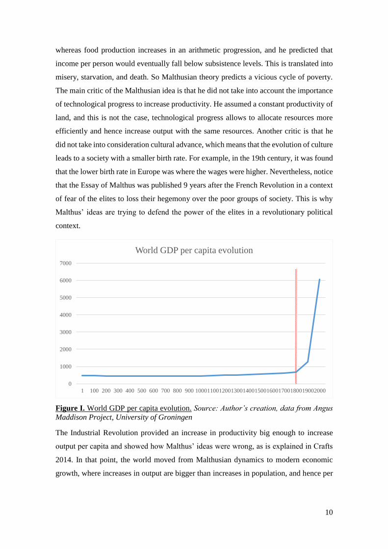
As Figure I shows, before the Industrial Revolution economic growth was small and
weak. Increases in per capita income were not possible because population and total
output were growing hand in hand at a very similar rate.
On the basis of this trend, Malthus’ established what is known as the Malthusian
Catastrophe. Thomas Robert Malthus is well known for his studies in demography and
mainly for his work An Essay on the Principle of Population, published in 1798. As it is
explained in Cypher 2014 Malthus theory states that increases in food production will
produce a temporary increase on the well-being, because rapidly population will grow
and the increase will be canceled by the increase in population, leading to the same per
capita production level, as we can see in Figure I. He argued the poor are responsible for
their own misery and that the increase in population responding to an improvement in
food is due to the animal nature, specifically the laboring poor, whom Malthus seem
morally inferior to the rich. So he states that the nature of the population is to increase
rather than maintaining higher standards of living, this is known as the Malthusian trap.
Malthus also explains how population increase is limited by the ability of the land to
produce enough food. He believed that population increased in a geometric progression
10
whereas food production increases in an arithmetic progression, and he predicted that
income per person would eventually fall below subsistence levels. This is translated into
misery, starvation, and death. So Malthusian theory predicts a vicious cycle of poverty.
The main critic of the Malthusian idea is that he did not take into account the importance
of technological progress to increase productivity. He assumed a constant productivity of
land, and this is not the case, technological progress allows to allocate resources more
efficiently and hence increase output with the same resources. Another critic is that he
did not take into consideration cultural advance, which means that the evolution of culture
leads to a society with a smaller birth rate. For example, in the 19th century, it was found
that the lower birth rate in Europe was where the wages were higher. Nevertheless, notice
that the Essay of Malthus was published 9 years after the French Revolution in a context
of fear of the elites to loss their hegemony over the poor groups of society. This is why
Malthus’ ideas are trying to defend the power of the elites in a revolutionary political
context.
Figure I. World GDP per capita evolution. Source: Author’s creation, data from Angus
Maddison Project, University of Groningen
The Industrial Revolution provided an increase in productivity big enough to increase
output per capita and showed how Malthus’ ideas were wrong, as is explained in Crafts
2014. In that point, the world moved from Malthusian dynamics to modern economic
growth, where increases in output are bigger than increases in population, and hence per
0
1000
2000
3000
4000
5000
6000
7000
1 100 200 300 400 500 600 700 800 900 10001100120013001400150016001700180019002000
World GDP per capita evolution

11
capita output can increase, as Figure I shows. Notice that in the graph, there is a vertical
bar denoting the Industrial Revolution.
Some years later, in the same context and at a mature stage of the first Industrial
Revolution, David Ricardo published the Principles of Political Economy and Taxation
1817. David Ricardo is one of the most influential economists, together with Adam Smith
or Karl Marx. He studied different fields in economy and his theory of comparative
advantage convinced the British government, together with Adam Smith ideas, to
promote free trade and globalization around the world. As is explained in Piketty Capital
in the XXIst Century David Ricardo establishes a relationship between economic growth
and inequality on the basis of the scarcity principle. Using Malthus’ ideas he assumed
that increases in output will imply increases in population and this will made land scarcer
the more output increases. This will make land prices constantly increase, together with
the rents of land and hence landowners will constantly receive a bigger amount of national
income. Since the rents received by the landowners constantly increase, there is less
income available for wages, as explained in Cypher 2014. In that sense, Ricardo
understood that inequality will be negatively affected by economic growth.
Like Ricardo, another economist that understood a negative relationship between growth
and inequality was Marx. Karl Marx devoted his life to understanding the dynamics of
the capitalist industrial society. As Prados de la Escosura 2015 indicates, the periods of
bigger economic growth are the ones with less social peace, because those periods
generate inequalities. Karl Marx saw the creation of the industrial capitalist society and
tried to give an explanation of the nature and the evolution of the capitalist system. The
new capitalist world was based on industrial capital rather than land, as Thomas Pikkety
describes in his book. For this reason, Marx modified the theory of Ricardo an adopted it
for a society where industrial capital was the new land, and the capitalists were the new
landowners. The main difference between industrial capital and land is that industrial
capital can be accumulated forever. For this reason, the conclusions of Marx were that
capital will accumulate forever and concentrate in fewer hands. Therefore, according to
Marx’ theory, economic growth understood as increases in output will provoke an
accumulation of capital but only on those that had the capital, and as a consequence
inequality will increase.

12
3.2. 20TH CENTURY-THE DATA REVOLUTION
No other interesting contributions were done to this issue until Simon Kuznets. In 1955
and in a post-war world, Simon Kuznets further developed this issue thanks to the new
improvements in data collection. He was the first one using data to check for the effect of
economic growth on inequality. During his studies, Kuznets used the GINI coefficient to
measure inequality, and GDP per capita to measure economic growth. As described in
Kuznets 1955, there are two main forces that increase inequality in the distribution of
income, analyzed before taxes. The first force is the fact that upper-income groups have
a higher saving rate and this will imply a constant concentration of income in upper-
income groups that will be transmitted to their descendants. This is also shown in Stiglitz
1969, where the author analyzed the distribution of income and wealth and generates a
model with different savings for the capitalists and the workers. The second force
according to Kuznets’ is the industrial structure of income distribution. Even if per capita
income is higher in industrial societies than in rural societies, inequalities are higher as
well. For this reason, the shift from rural to industrial societies generates an increase in
the overall inequality. Kuznets’ was very interested in the shift from agricultural to an
industrial society and its effect on inequality. What Kuznets found was the so-called
Kuznets curve. It implies that the relationship between economic growth and income
inequality has an inverted U shape. As it is described in his work, the pattern of income
inequality is to increase in the first stages of economic growth during the transition from
pre-industrial to industrial societies, stabilize, and then decrease in the more developed
stages of growth. This is because in the first stages of industrialization the income
distribution of the urban population was more unequal than that of the agricultural. To
explain the shift from increasing to decreasing inequality Kuznets’ had two main points.
The first one is that the movement from rural areas to industrial areas have implied an
increase in the income received by the low-income population from industrial areas. The
second point is that development creates democracies, and in democratic societies the
interest of the low-income groups are better represented, leading to a more protective and
redistributive policies that counteract the effects of industrialization. Kuznets’ also adds
that the functioning of a free economic society will counteract the negative effect of the
concentration of savings on inequality.
In conclusion, Kuznets’ hypothesis states that the first stages of industrialization will
increase inequality, but the later stages will make it decrease. This is why it follows an
13
inverted “U” shape over the course of industrialization. So Kuznets provides a very
optimistic evolution and a strong confidence in economic growth. However, as Kuznets
pointed out “The paper is perhaps 5 per cent empirical information and 95 per cent
speculation, some of it possibly tainted by wishful thinking” (Kuznets 1955. p.26)
Despite the fact that Kuznets was the first economist talking about inequality with
empirical information, he was not taking into account exogenous shocks in the reduction
of inequality, as it is described by Thomas Piketty in Capital of the XXIst Century. Piketty
warns the reader that the period that Kuznets understood as the one with reductions in
inequality was, in fact, the Great Depression and World War II. Moreover, Piketty
emphasizes how Kuznets’ conclusions could be politically influenced. His theory was
justifying the no intervention into the market.
3.3.21ST CENTURY- THE WORLD AFTER KUZNETS
The Kuznets hypothesis was valid for the US and OECD countries until the 1970s, as is
pointed in Aghion, Caroli and García-Peñalosa 1999. Their work describes that before
the 70s, it appeared to be a virtuous cycle were low inequality incentivized growth and
this growth reduced inequality. However, after the 70s as both Aghion, Caroli and
García-Peñalosa 1999 and Piketty 2014 explain, inequality in rich countries increased
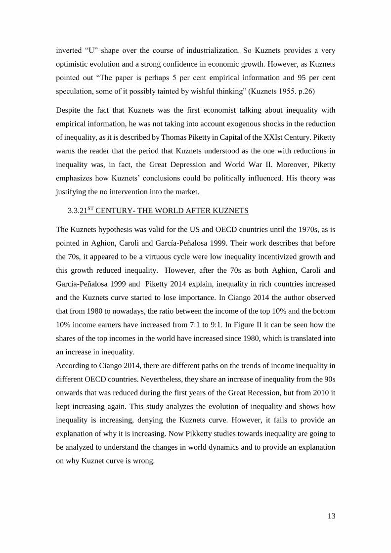
and the Kuznets curve started to lose importance. In Ciango 2014 the author observed
that from 1980 to nowadays, the ratio between the income of the top 10% and the bottom
10% income earners have increased from 7:1 to 9:1. In Figure II it can be seen how the
shares of the top incomes in the world have increased since 1980, which is translated into
an increase in inequality.
According to Ciango 2014, there are different paths on the trends of income inequality in
different OECD countries. Nevertheless, they share an increase of inequality from the 90s
onwards that was reduced during the first years of the Great Recession, but from 2010 it
kept increasing again. This study analyzes the evolution of inequality and shows how
inequality is increasing, denying the Kuznets curve. However, it fails to provide an
explanation of why it is increasing. Now Pikketty studies towards inequality are going to
be analyzed to understand the changes in world dynamics and to provide an explanation
on why Kuznet curve is wrong.
14
Figure II. World Top Income Shares Evolution.Source: Author’s creation, data from
World Inequality Database
After Simon Kuznets hypothesis was proven to be wrong, a new group of economists
started to analyze the relationship between economic growth and inequality. This is the
case of Thomas Piketty, that has devoted his life to understand the dynamics of income
and wealth distribution and has done enormous contributions to the debate. In Piketty and
Saez 2001, a lot of new data was provided to study this issue. For Piketty and Saez,
Kuznets’ conclusions were wrong. The relationship of inequality and economic growth
does not follow an inverted “U” shape because the observed decrease of inequality
interpreted by Simon Kuznets corresponded to the period of the Great Depression and the
World Wars. So they state Kuznets curve is wrong because Kuznets was not taking into
account the effect on the labor market and on economic policy regarding inequality that
the Great Depression and the World Wars produced. This is exemplified with strongly
distributive policies and the rise of the unions. In their work, Piketty and Saez, explain
how this period generated a destruction of business and this reduced the share of top
capital incomes, reducing inequality. They observed a relationship between economic
growth and inequality depended on wages, or on tax systems.
For Piketty, inequality decreases in the periods of higher taxation, such as during WWI
and WWII and increases in periods of low taxation, such after the Tax Reform Act 1986.
In Piketty 2014 the author explains the importance of the role of progressive taxation and
15%
16%
17%
18%
19%
20%
21%
22%
23%
45%
47%
49%
51%
53%
55%
57%
1980198219841986198819901992199419961998200020022004200620082010201220142016
World Top Income Shares Evolution
World 10% World 1%

15
states that taxes allow for collective action in society. He explains how progressive
taxation was created during WWI and WWII with the need of finance the war.
Nevertheless, even if it was created due to war, for Piketty the progressive income tax is
the main fiscal innovation of the century, and it is a mechanism to reduce inequality. This
is why for Piketty the decrease in taxation after the 80s in the US and UK explains the
increase in top income shares. As Figure III shows, in the case of the UK, the relationship
is very clear, decreases in top income taxes imply increases in the Gini coefficient. Notice
this graph has a vertical line denoting the monetarist revolution of the 80s, that started a
bit earlier in the UK, as the graph itself shows. Figure IV also shows the same relationship
but for the US and France. This decrease in taxation is explained in the book of Kaufmann
and Stützle 2017. From this book, the 80s was the starting point of the so-called neoliberal
age. From this year onwards a period described by Kaufmann and Stützle 2017 as tax
competition era between states implied the reduction of taxes. As Table I shows, the
tendency of the top marginal income taxes from 1979 onwards is decreasing.
Apart from taxation, there are other redistributive tools, such as fixing maximum salaries
to reduce inequality on income, and Piketty exemplified this with what some European
economies did after WWII by making public firms and establishing the salaries. As we
can see in Figure IV, in the case of the US and France in the periods of higher taxation
the share of the top 10% income was reduced, and from the 80s onwards the tendency is
increasing. However, in Piketty and Saez 2001 both authors concluded that even though
taxes have an important effect on inequality, there are other factors that explain inequality.
Furthermore, they propose that shocks in capital income were responsible for the decrease
in inequality. So for Piketty, capital ownership is what really generates inequality.
Top Marginal Income Tax Rate (%)
Country 1979 1990 2002 Country 1979 1990 2002
Belgium 76 55 52 France 60 52 50
Brazil 55 25 28 Germany 56 53 49
Chile 60 50 43 Japan 75 50 50
Denmark 73 68 59 Netherlands 72 60 52
Egypt 80 65 40 United Kingdom 83 40 40
Finland 71 43 37 United States 73 33 39
Table I. Top Marginal Income Tax Rate (%) Source: Author’s creation, data from
Alan Reynolds. "Marginal Tax Rates."

16
Figure III. UK Evolution of Marginal Top Income Tax and Gini Coefficient Source:
Author’s creation, data from All the Ginis Dataset (Gini coefficient), Thomas Piketty
Capital in the XXIst Century (Top Marginal Income Tax Rate) Retrieved from:
http://piketty.pse.ens.fr/fr/capital21C
Figure IV.US and France Top Marginal Income Tax Rate and Share Top 10% Income
Earners Evolution. Source: Author’s creation, data from World Inequality Database
(Shares of Top 10% Income) and Thomas Piketty Capital in the XXIst Century (Top
Marginal Income Tax Rates). Retrieved from http://piketty.pse.ens.fr/fr/capital21C
20
22
24
26
28
30
32
34
36
38
40
0%
20%
40%
60%
80%
100%1
90
0
19
04
19
08
19
12
19
16
19
20
19
24
19
28
19
32
19
36
19
40
19
44
19
48
19
52
19
56
19
60
19
64
19
68
19
72
19
76
19
80
19
84
19
88
19
92
19
96
20
00
20
04
20
08
20
12
UK Tax GINI Relationship
U.K. Top Tax Rate UK gini
0%
10%
20%
30%
40%
50%
60%
70%
80%
90%
190
0
190
4
190
8
191
2
191
6
192
0
192
4
192
8
193
2
193
6
194
0
194
4
194
8
195
2
195
6
196
0
196
4
196
8
197
2
197
6
198
0
198
4
198
8
199
2
199
6
200
0
200
4
200
8
201
2
Tax Rate Income Share Relationship
U.S. France France10% US10%
17
After having proven how Kuznets curve is wrong, Piketty does his own interpretation of
the economic growth/inequality relationship in his controversial book Capital in the 21st
Century. Piketty notices that there are forces of convergence and forces of divergence
towards inequality. The main force of divergence is what he calls the First Fundamental
Law of Capitalism. This law implies that r>g and, where r is the average annual rate of
return on capital, and g is the rate of growth of the economy. This law is assumed to be
true for the last 2000 years of history. Before the industrial revolution, g was zero and
hence r was larger. After the industrial revolution and in the actual trends, r has a value
between 4% and 5%, and the long term rate of growth of the economies is around 2%.
The intuition is the following
When the rate of return on capital significantly exceeds the growth rate of the
economy […], then it logically follows that inherited wealth grows faster than
output and income. People with inherited wealth need to save only a portion of
their income from capital to see that capital grow more quickly than the economy
as a whole. (Piketty 2013. p. 34)
Moreover, Piketty ads that there are mechanisms to reinforce this divergence such as
higher level of saving rates for higher owners of wealth.
Piketty puts very importance on the capital/income ratio together with the national
division of income between labor and capital and shows how it has recovered historical
levels, and it will keep increasing. This means capital is having more importance in the
economy. This is why the second divergence mechanism is what he calls the Second
Fundamental Law of Capitalism. This law says that in the long run B=s/g. Where B is the
capital/income ratio of an economy, this is, the level of national capital; s is the savings
rate of the economy, and g is the growth rate. Extracted from the book:
[…]a country that saves a lot and grows slowly will over the long run accumulate
an enormous stock of capital, which in turn can have significant consequences on
the social structure and distribution of wealth. [...] In a quasi-stagnant society,
wealth accumulated in the past will inevitably acquire disproportionate
importance. (Piketty 2013. p. 207.)
He suggest the possible solution for the fundamental law of capitalism is a progressive
global tax on capital to reduce the level of capital accumulation of the capitalists and it is
justified by saying that this tax would have dynamics effects on the economy by reducing

18
the return obtained from wealth, and hence, helping reduce this vicious cycle of wealth
accumulation that generates inequality. Piketty also adds that this progressive tax on
capital should be accompanied by a high level of international transparency. However,
Piketty assumes this global tax on capital is a utopian idea and suggests it should be
implemented progressively, with countries wishing to do it.
Piketty theory has been controversial and there are a lot of critics to his view. As described
in Kaufmann and Stützle 2017
[…]Piketty analysis attacked some of the cornerstones of neoliberal ideology: that
the market is a merely neutral place in which everyone can in principle pursue and
find happiness; that differences in income and wealth are to be welcomed, since
they motivate individuals to achieve; and that this differences are legitimate, since
they reflect different levels of performance or preferences of market-individuals.
(Kaufmann and Stützle 2017. p.43.).
One of those critics is the one done by Gregory Mankiw. In Mankiw 2015 the author
analyzes what Piketty calls the first fundamental law of capitalism using an expansion of
the Solow growth model. He is not surprised by the fact that r>g and he says that:
In this model, r>g is not a problem, but r<g could be. If the rate of return is less
than the growth rate, the economy has accumulated an excessive amount of
capital. In this dynamically inefficient situation, all generations can be made better
off by reducing the economy’s saving rate. From this perspective, we should be
reassured that we live in a world in which r>g because it means we have not left
any dynamic Pareto improvements unexploited. (Mankiw 2015. p.1)
So what for Piketty seems an unavoidable catastrophe, for Mankiw, is a necessary
condition for the well-functioning of the economy.
Mankiw predicts that if r>g, there will be a steady state level of inequality, measured with
the ratio between the consumption of the workers and the consumption of the capitalists,
denoted Cw/Ck. He shows that a higher capital tax will improve the ratio, but by reducing
the consumption of both workers and capitalists. This is why the solution Mankiw
proposes is a progressive tax on consumption. He believes this tax could reduce
consumption inequality between capitalist and workers without discouraging capital
accumulation.

19
So even if Piketty has done enormous contributions to understand inequality, its sources
and its evolution, the neoclassical school seems not to like his theory.
3.4.OVERALL REVISION
The aim of this part of the work is to put together the different theories of inequality
analyzed and try to find a proxy to test them in the next section.
AUTHOR THEORY DEFINITION PROXY
David Ricardo
Karl Marx
Principle of scarcity The scarcity of capital
will make capital
owners accumulate
more wealth the more
the economy
increases.
Simon Kuznets The inverted “U”
curve
Inequality will
increase in the first
stages of
development and
later will decrease.
Importance of saving
rates on the upper
groups.
Urbanization rate
Saving rate
Thomas Piketty r>g and B=s/g Under this condition,
inherited wealth takes
more importance
every period,
generating inequality.
Importance on the
welfare state, taxation
and redistribution on
reducing inequality
Expenditure to
GDP rate

20
4. DATA
After having reviewed the existing literature surrounding this issue, the objective of this
part of the work is to check the hypothesis of this work. Does economic development
have an effect on the distribution of income?
To check for the distribution of income different indicators are going to be used. The main
indicator is the Gini coefficient, but top shares of 1% income owners and 10% income
owners, as well as the bottom 50% income share, are also going to be used. In the first
place, the aim of this work was to do a cross-country analysis, using panel data from all
possible countries in the world. However, it is difficult to find historical data for the GINI
coefficient and distribution of income, so this has importantly reduced our possibilities of
analysis. The main two sources for Gini coefficient data are the All The Ginis Database
done by the World Bank Data and the World Income Inequality Database created by the
United Nations University.
All The Ginis Database includes combined and standardized Ginis from different sources.
In Milanovic 2014, where Branko Milanovic does an analysis of this database, it is said
that the column Giniall of the database should be comparable. This column includes the
standardized Gini coefficients of most countries in the world, covering different periods.
Actually, it is the column used in the work of Li and Zhou 2013, where they tested for the
effect of economic growth on the Gini coefficient. However, Milanovic warns the reader
that the Ginis of this database may be calculated used different mathematical methods
and geometrical approximations to the Lorenz curve and this can create differences on
the values. For this reason, Milanovic warns that the results of using this database can be
biased. To avoid the problem just described, this database has not been used in the
analysis.
The other important database is the World Income Inequality Database that provides Gini
index from all available sources. However, as UNU-WIDER (2018)2 points outs this
database is different from national databases and the observations are not comparable.
This is because the methodology used in the computations is different for different
countries and also for different years in the same country, and the results are not
standardized. As we can see, the World Income Inequality Database does not provide
2 Notice this is the user guide of the World Income Inequality Database

21
standardized values for the Gini coefficient and makes its comparability impossible
without a deep and complex adjustment.
In conclusion, even if there is access to the biggest two data sets on income distribution,
Ginis provided are not comparable and hence some adjustments need to be done. Since
these adjustments imply a very deep understating of the techniques used to compute the
values another database is going to be used in this analysis. Also, it is important to
consider the study of Atkinson and Brandolini (2001) where the authors warn about the
risk of using secondary datasets and how they can lead to erroneous results. For this
reason, the database that will be used is the Gini coefficient of equalized disposable
income obtained from the EU-SILC survey done by Eurostat. This data set includes
observations of EU countries from 1995 to 2018. Since all the observations are computed
by Eurostat, they are comparable and can be used in the analysis. From now on, for the
rest of the variables, the data used will be from EU countries and the period of time from
1995 to 2018.
The other proxies of income distribution used in this analysis are the shares of income as
a percentage of total income received by the top 1 %, the top 10%, and the bottom 50%
income receivers. The data of these variables are obtained from the World Inequality
Database.3
The main independent variable is the evolution of economic development measured in
terms of GDP per capita. The variable used is GDP per capita PPP in current international
dollars and it is obtained from World Bank Data. Notice this variable has been divided
by 1000 and GDP is expressed in thousands of dollars, this is to eliminate decimals in the
values of the parameters. The other control variables that will be used, also obtained from
World Bank Data, are GDP per capita growth (annual %), inflation measured by
consumer prices (annual %), GDP gross domestic savings (% of GDP) and urban
population (% of total population). Total general government expenditure (% of GDP) is
also going to be used as a control variable and it has been obtained from Eurostat.
Once all the data has been obtained and analyzed together, the countries that lacked more
information have been eliminated from the analysis to provide a more robust conclusion.
3 As described on its website “The World Inequality Database (WID.world) aims to provide open and
convenient access to the most extensive available database on the historical evolution of the world
distribution of income and wealth, both within countries and between countries.”
22
So eventually, the data set used for this analysis includes information of the variables
mentioned before from Austria, Belgium, Bulgaria, Cyprus, Czechia, Denmark, Estonia,
Finland, France, Germany, Greece, Hungary, Iceland, Ireland, Italy, Latvia, Lithuania,
Luxembourg, Netherlands, Norway, Poland, Portugal, Romania, Slovakia, Slovenia,
Spain, Sweden, Switzerland and United Kingdom.
5. METHODOLOGY
The statistical model used in the analysis is a linear mixed effect model. The variable
“Country” has been established as random because there are repeated measures on it, that
is, for each country there are different years. The fixed part of the model includes different
dependent variables (Gini, top1%, top10% and bottom50%) Moreover, the variable
selection process used has been a sequential strategy by which the first regression includes
the dependent variable (Gini, top1%, top10% or bottom 50%) to GDP per capita, and then
the other control variables have been added to the model one by one checking its results
and significance. Since 4 different dependent variables have been analyzed (Gini, top1%,
top10%, or bottom 50%) and there were 6 independent variables, 7 taking into account
that an interaction variable between GDP per capita and GDP growth has been created, a
total amount of 24 models have been produced. For simplicity of the work, only the more
relevant models will be shown in the results. Notice that the significance of the variables
has been analyzed by looking at the ANOVA test of each model and analyzing the p-
value. The use of ANOVA test in analyzing the significance of a parameter of a linear
mixed effect model is suggested by Pinheiro and Bates 2006.
Before starting with the analysis, a Pearson correlation matrix has been produced to
measure the linear correlation between variables and avoid regressing variables that are
highly correlated. See Pearson 1909. Table II shows the results of Pearson correlation
matrix. As we can see in Table II, variables of top and bottom shares are highly correlated
among them and in relationship to Gini, this is why those variables have not been used as
control variables when Gini was the dependent variable. The other worrisome correlation
is the one between gross domestic savings and GDP per capita, that has a value of (0,68).
However, after testing for the effect of savings in the model, it has been considered
acceptable and hence, included in the analysis.

23
Pearson Correlation Matrix
gini gov_exp gdp savings gdp_growth
gini 1 -0,04 -0,32 -0,42 0,08
gov_exp -0,04 1 0,02 -0,02 -0,18
gdp -0,32 0,02 1 0,68 -0,22
savings -0,42 -0,02 0,68 1 0,11
gdp_growth 0,08 -0,18 -0,22 0,11 1
urban_pop -0,26 -0,32 0,44 0,18 -0,17
inflation 0,03 -0,01 -0,3 -0,16 0,15
Top1.Share 0,27 -0,21 0,07 0 0,09
Top10.Share 0,57 -0,14 -0,04 -0,17 0,11
Bottom50.share -0,64 0,06 0,07 0,25 -0,09
urban_pop inflation Top1.Share Top10.Share Bottom50.share
gini -0,26 0,03 0,27 0,57 -0,64
gov_exp -0,32 -0,01 -0,21 -0,14 0,06
gdp 0,44 -0,3 0,07 -0,04 0,07
savings 0,18 -0,16 0 -0,17 0,25
gdp_growth -0,17 0,15 0,09 0,11 -0,09
urban_pop 1 -0,16 0,04 -0,06 -0,01
inflation -0,16 1 -0,14 -0,11 0,12
Top1.Share 0,04 -0,14 1 0,84 -0,56
Top10.Share -0,06 -0,11 0,84 1 -0,85
Bottom50.share -0,01 0,12 -0,56 -0,85 1
Table II. Pearson Correlation Matrix of the Dataset Utilized in the Analysis. Source:
Author’s creation
6. RESULTS AND INTERPRETATION
The first model produced is a very basic model in which the effect of GDP per capita on
the Gini coefficient has been tested. The same has been done testing the effect of GDP
per capita in top1% income share, top 10% income share, and bottom 50% income share.
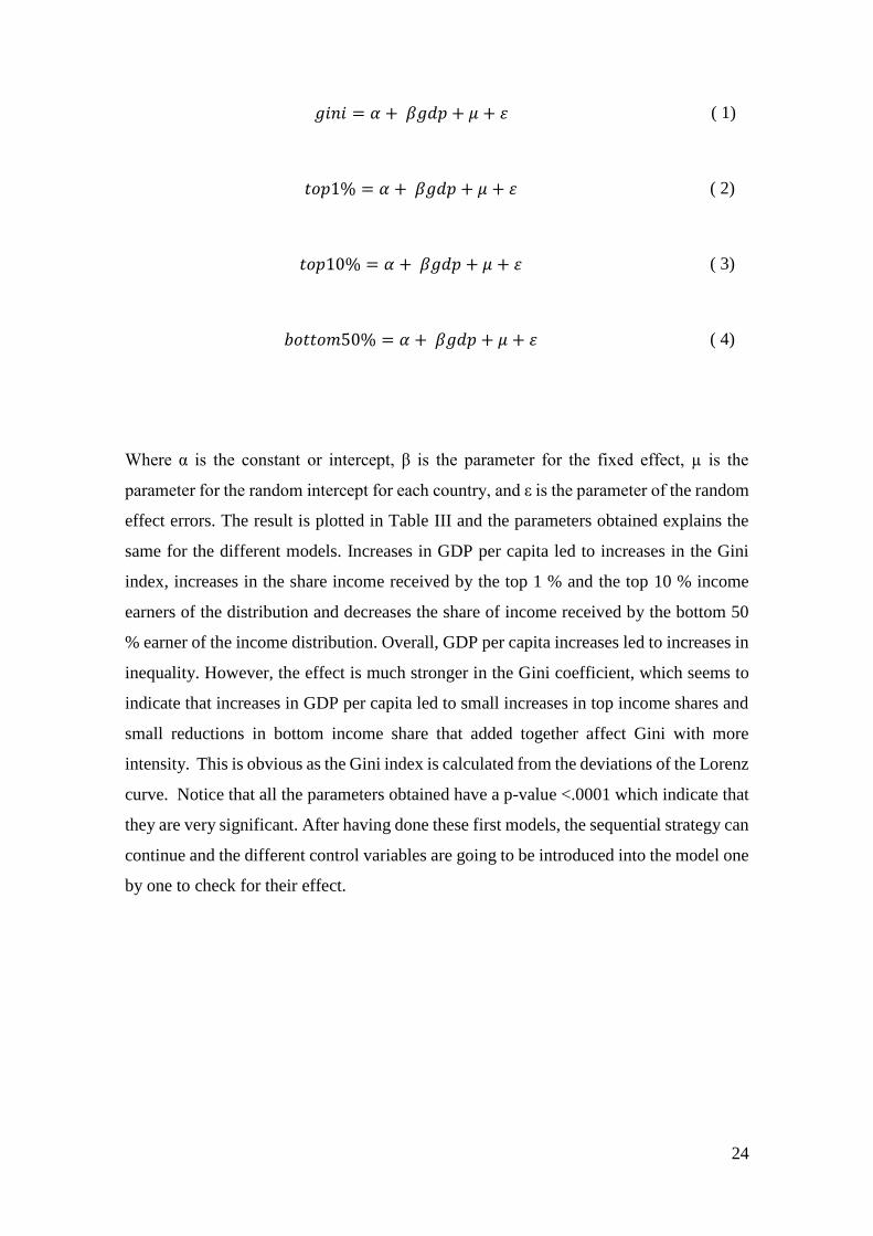
The models follow the next equations:
24
𝑔𝑖𝑛𝑖 = 𝛼 + 𝛽𝑔𝑑𝑝 + 𝜇 + 𝜀
( 1)
𝑡𝑜𝑝1% = 𝛼 + 𝛽𝑔𝑑𝑝 + 𝜇 + 𝜀
( 2)
𝑡𝑜𝑝10% = 𝛼 + 𝛽𝑔𝑑𝑝 + 𝜇 + 𝜀
( 3)
𝑏𝑜𝑡𝑡𝑜𝑚50% = 𝛼 + 𝛽𝑔𝑑𝑝 + 𝜇 + 𝜀
( 4)
Where α is the constant or intercept, β is the parameter for the fixed effect, µ is the
parameter for the random intercept for each country, and ε is the parameter of the random
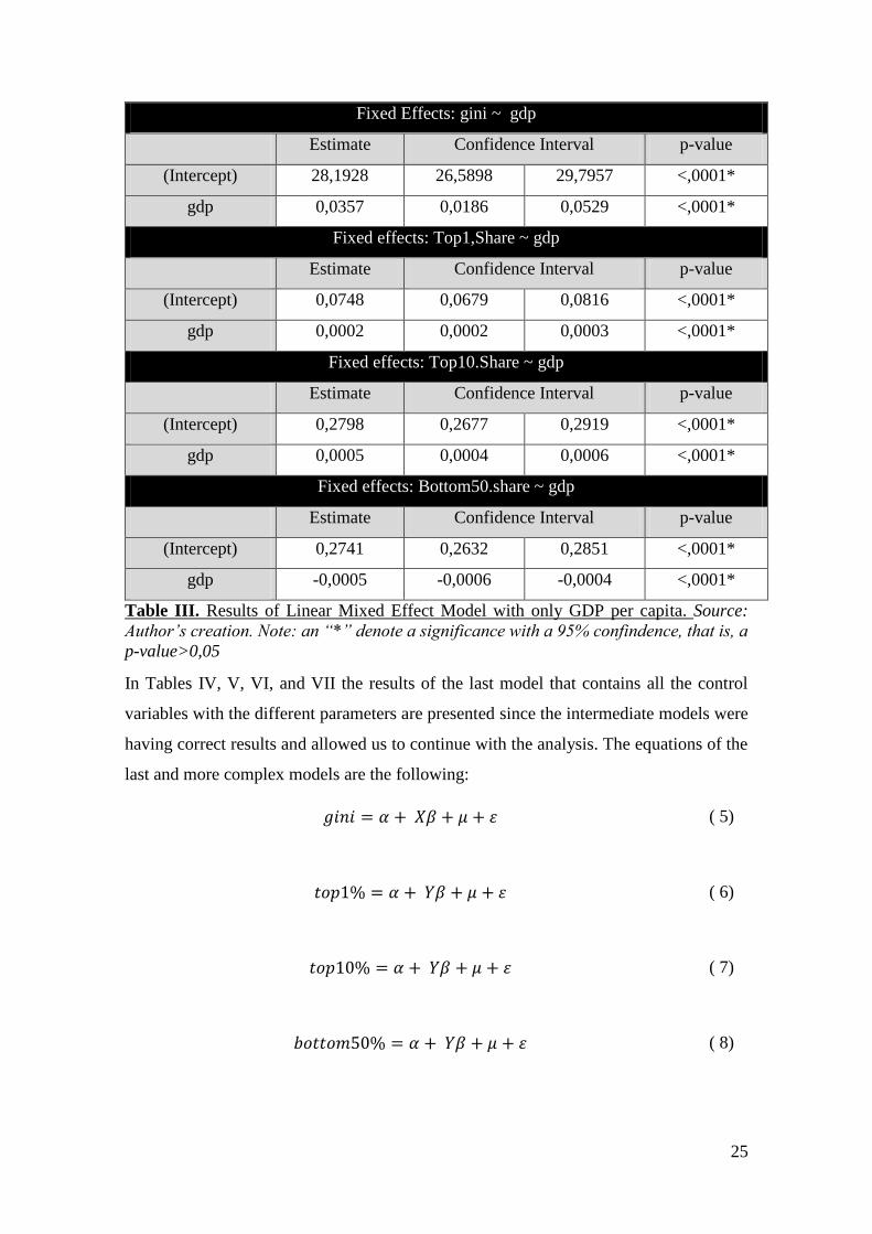
effect errors. The result is plotted in Table III and the parameters obtained explains the
same for the different models. Increases in GDP per capita led to increases in the Gini
index, increases in the share income received by the top 1 % and the top 10 % income
earners of the distribution and decreases the share of income received by the bottom 50
% earner of the income distribution. Overall, GDP per capita increases led to increases in
inequality. However, the effect is much stronger in the Gini coefficient, which seems to
indicate that increases in GDP per capita led to small increases in top income shares and
small reductions in bottom income share that added together affect Gini with more
intensity. This is obvious as the Gini index is calculated from the deviations of the Lorenz
curve. Notice that all the parameters obtained have a p-value <.0001 which indicate that
they are very significant. After having done these first models, the sequential strategy can
continue and the different control variables are going to be introduced into the model one
by one to check for their effect.
25
Fixed Effects: gini ~ gdp
Estimate Confidence Interval p-value
(Intercept) 28,1928 26,5898 29,7957 <,0001*
gdp 0,0357 0,0186 0,0529 <,0001*
Fixed effects: Top1,Share ~ gdp
Estimate Confidence Interval p-value
(Intercept) 0,0748 0,0679 0,0816 <,0001*
gdp 0,0002 0,0002 0,0003 <,0001*
Fixed effects: Top10.Share ~ gdp
Estimate Confidence Interval p-value
(Intercept) 0,2798 0,2677 0,2919 <,0001*
gdp 0,0005 0,0004 0,0006 <,0001*
Fixed effects: Bottom50.share ~ gdp
Estimate Confidence Interval p-value
(Intercept) 0,2741 0,2632 0,2851 <,0001*
gdp -0,0005 -0,0006 -0,0004 <,0001*
Table III. Results of Linear Mixed Effect Model with only GDP per capita. Source:
Author’s creation. Note: an “*” denote a significance with a 95% confindence, that is, a
p-value>0,05
In Tables IV, V, VI, and VII the results of the last model that contains all the control
variables with the different parameters are presented since the intermediate models were
having correct results and allowed us to continue with the analysis. The equations of the
last and more complex models are the following:
𝑔𝑖𝑛𝑖 = 𝛼 + 𝑋𝛽 + 𝜇 + 𝜀
( 5)
𝑡𝑜𝑝1% = 𝛼 + 𝑌𝛽 + 𝜇 + 𝜀
( 6)
𝑡𝑜𝑝10% = 𝛼 + 𝑌𝛽 + 𝜇 + 𝜀
( 7)
𝑏𝑜𝑡𝑡𝑜𝑚50% = 𝛼 + 𝑌𝛽 + 𝜇 + 𝜀
( 8)
26
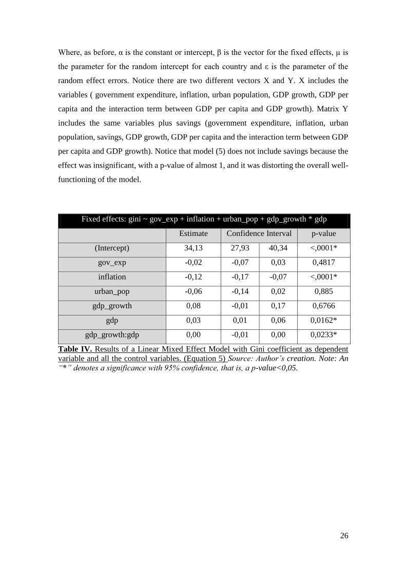
Where, as before, α is the constant or intercept, β is the vector for the fixed effects, µ is
the parameter for the random intercept for each country and ε is the parameter of the
random effect errors. Notice there are two different vectors X and Y. X includes the
variables ( government expenditure, inflation, urban population, GDP growth, GDP per
capita and the interaction term between GDP per capita and GDP growth). Matrix Y
includes the same variables plus savings (government expenditure, inflation, urban
population, savings, GDP growth, GDP per capita and the interaction term between GDP
per capita and GDP growth). Notice that model (5) does not include savings because the
effect was insignificant, with a p-value of almost 1, and it was distorting the overall well-
functioning of the model.
Fixed effects: gini ~ gov_exp + inflation + urban_pop + gdp_growth * gdp
Estimate Confidence Interval p-value
(Intercept) 34,13 27,93 40,34 <,0001*
gov_exp -0,02 -0,07 0,03 0,4817
inflation -0,12 -0,17 -0,07 <,0001*
urban_pop -0,06 -0,14 0,02 0,885
gdp_growth 0,08 -0,01 0,17 0,6766
gdp 0,03 0,01 0,06 0,0162*
gdp_growth:gdp 0,00 -0,01 0,00 0,0233*
Table IV. Results of a Linear Mixed Effect Model with Gini coefficient as dependent
variable and all the control variables. (Equation 5) Source: Author’s creation. Note: An
“*” denotes a significance with 95% confidence, that is, a p-value<0,05.

27
Fixed effects: Top1.Share ~ gov_exp + inflation+ urban_pop + gdp_growth * gdp
Estimate Confidence Interval p-value
(Intercept) 0,001 0,001 0,000 <,0001*
gov_exp -0,07 -0,09 -0,04 <,0001*
inflation 0,16 -2,91 0,34 0,4355
urban_pop 0,97 -0,03 0,05 0,0014*
savings -0,02 -0,06 0,77 0,0427*
gdp_growth 0,06 0,01 0,00 0,0061*
gdp 0,03 0,02 0,05 <,0001*
gdp_growth:gdp -0,09 -0,13 0,13 0,9896
Table V. Results of a Linear Mixed Effect Model with Top1% Income Share as
dependent variable and all the control variables.(Equation 6) Source: Author’s creation.
Note: An “*” denotes a significance with 95% confidence, that is, a p-value<0,05
Fixed effects: Top10.Share ~ gov_exp + inflation + urban_pop + gdp_growth *gdp
Estimate Confidence Interval p-value
(Intercept) 0,00003 0,00003 0,00004 <,0001*
gov_exp -0,09 0,00 -0,05 <,0001*
inflation 0,14 -0,13 0,42 0,9677
urban_pop 0,02 -0,05 0,08 <,0001*
savings -0,05 0,00 -0,48 0,0236*
gdp_growth 0,08 0,02 0,00 0,007*
gdp 0,06 0,05 0,08 <,0001*
gdp_growth:gdp -0,14 -0,14 0,25 0,594
Table VI. Results of a Linear Mixed Effect Model with Top10% Income Share as
dependent variable and all the control variables.(Equation 7) Source: Author’s creation.
Note: An “*” denotes a significance with 95% confidence, that is, a p-value<0,05

28
Fixed effects: Bottom50.share ~ gov_exp + inflation+ urban_pop + gdp_growth *gdp
Estimate Confidence Interval p-value
(Intercept) 0,00003 0,00003 0,00003 <,0001*
gov_exp 0,04 0,94 0,06 0*
inflation_consumer 0,71 -0,13 0,27 0,0635*
urban_pop -0,06 0,00 -0,01 <,0001*
savings 0,02 -0,02 0,05 0,0004*
gdp_growth -0,05 -0,09 0,03 0*
gdp -0,05 -0,06 -0,03 <,0001*
gdp_growth:gdp -0,35 -0,18 0,11 0,6306
Table VII. Results of a Linear Mixed Effect Model with Bottom 50% Income Share as
dependent variable and all the control variables.(Equation 8) Source: Author’s creation.
Note: An “*” denotes a significance with 95% confidence, that is, a p-value<0,05
Now that the models have been presented, an analysis of each variable is going to be
done, trying to understand the values obtained in the regressions.
6.1.GDP PER CAPITA
Testing the effect of GDP per capita on inequality is the main objective of this work. The
parameters obtained in the regression show that, after introducing all the control variables
into the model, GDP per capita still have a significant effect on income inequality (see
Tables IV, V, VI, and VII). The process of economic development during the years 1995
and 2018 has had a negative impact on income inequality in the European countries
analyzed. As Figures V, VI, VII, and VIII4 show, for higher values of GDP per capita,
higher is the value of the Gini coefficient, higher is the income share obtained by the top
1% and top 10% income earners of the society, and lower is the share obtained by the
bottom 50% income earner, i.e., higher values of GDP per capita imply higher income
inequality. Figures V, VI, VII and VIII are proof of the hypothesis proposed on this work:
the process of economic development does have a negative impact on income inequality.
4 Figures V,VI, VII, and VIII displays the average of the countries analyzed during each year for the Gini
coefficient; the top 1%, 10% and bottom 50% shares; and the GDP per capita. The average has been
called European average, even though some European countries are missing in the computations.

29
Figure V. Scatter Plot of the European Average GDP per capita and Gini Index (1997-
2016). Source: Author’s creation, data from Eurostat (Gini) and World Bank Data(GDP
per capita). Note: The average only includes the countries analyzed in this work, is not
the total European average, but a good representative.
Figure VI. Scatter Plot of the European Average GDP per capita and Average Top 1%
Income Share (1997-2016). Source: Author’s creation, data from Eurostat (Gini) and
World Inequality Database(Top 1% share). Note: The average only includes the countries
analyzed in this work, is not the total European average, but a good representative.
27
27,5
28
28,5
29
29,5
30
14000 19000 24000 29000 34000 39000
Aver
age
Gin
i In
dex
Average GDP per capita
Gini Index- GDP per capita Evolution
Evuropean Average (1997-2016)
0,072
0,075
0,078
0,081
0,084
0,087
14000 19000 24000 29000 34000 39000
Aver
age
shar
e to
p 1
%
Average GDP per capita
Top 1% Income Share - GDP per capita
European Average (1996-2016)

30
Figure VII. Scatter Plot of the European Average GDP per capita and Average Top 10%
Income Share (1997-2016). Source: Author’s creation, data from Eurostat (Gini) and
World Inequality Database (Top 10% Share). Note: The average only includes the
countries analyzed in this work, is not the total European average, but a good
representative.
Figure VIII. Scatter Plot of the European Average GDP per capita and Average Bottom
50% Income Share (1997-2016). Source: Author’s creation, data from Eurostat (Gini)
and World Inequality Database (Bottom 50% Share). Note: The average only includes
the countries analyzed in this work, is not the total European average, but a good
representative.
0,275
0,28
0,285
0,29
0,295
0,3
0,305
14000 19000 24000 29000 34000 39000
Aver
age
shar
e to
p 1
0%
Average GDP per capita
Top 10% Income Share - GDP per capita
European Average (1996-2016)
0,244
0,248
0,252
0,256
0,26
0,264
0,268
14000 19000 24000 29000 34000 39000
Aver
age
shar
e b
ott
om
50
%
Average GDP per capita
Bottom 50% Income Share - GDP per capita
European Average (1996-2016)
31
From Tables IV, V, VI, and VII different conclusions can be extracted. On the first place,
GDP per capita has a significant effect on the Gini coefficient with a p-value on the
ANOVA test of (0,0162). However, the significance increases if we take a look at the
effect of GDP per capita on income shares. In that case, the p-values are (<,0001) in the
three models. So GDP per capita increases top income shares and decreases bottom
income shares in a small portion, which led to an overall higher effect on the Gini
coefficient.
To understand the diffusion mechanism through which economic development affects
income inequality Piketty 2013 and what he calls the first fundamental law of capitalism
should be considered. This “law” says that if the return on capital is higher than economic
growth, then wealth owners will see their wealth increase faster than the total output of
the economy, and hence, inequality will increase. In Table VIII the average GDP per
capita growth is shown for every country analyzed in this work. It can be seen that only
Estonia, Ireland, Latvia, Lithuania, and Poland have had an average growth above 4%.
Moreover, none of the countries have had an average growth higher than 6%. To check
for Piketty’s fundamental law, now the values for the average return on capital are needed.
However, those values are very difficult to find and it will require a whole work just to
find the values for each country. Nevertheless, there are some studies that can be used. In
Canales, Lau, Lee, Maneti and Owada 2017 the authors found the average rate of return
on capital for the periods 2013-2015 of different countries. Germany (9.1%), Finland
(8.3%), Czechia (10%) and Greece (9%). Moreover, in Value Trust 2018 the authors
computed the implied capital market return on Europe at every year between 2012 and
2018, and the values fluctuate between 9.5% and 7.7%.

32
Average (%) GDP per capita growth rate per year 1995-2018
Country
Average
Growth Country
Average
Growth Country
Average
Growth
Austria 1,405 Greece 0,745 Poland 4,202
Belgium 1,290 Hungary 2,493 Portugal 1,201
Bulgaria 3,677 Iceland 2,442 Romania 3,820
Cyprus 1,375 Ireland 4,684 Slovakia 3,993
Czechia 2,552 Italy 0,366 Slovenia 2,390
Denmark 1,148 Latvia 5,301 Spain 1,442
Estonia 4,669 Lithuania 5,507 Sweden 2,021
Finland 1,931 Luxembourg 1,712 Switzerland 1,006
France 1,050 Netherlands 1,586
United
Kingdom 1,576
Germany 1,383 Norway 1,318
Table VIII. Average (%) GDP per capita growth rate per year 1995-2018. Source:
Author’s creation. Data from Eurostat.
If it is assumed that those studies are representative of the rate of return on capital, it can
be concluded that the mechanism through which GDP per capita affects income inequality
is Piketty’s first fundamental law of capitalism. It is on the nature of the capitalist
economy to have a higher rate of return on capital than the rate of growth of the economy,
and as Piketty 2013 explains, this creates inequality. Nevertheless, there are other
variables that affect income inequality during the process of economic development,
some of them are the control variables utilized in this study. For this reason, to understand
mechanisms others apart from Piketty’s law, an analysis of the control variables used in
this study is needed.
6.2.GDP GROWTH
By analyzing GDP per capita, the effect of a determined level of GDP per capita on
income inequality is analyzed. However, now GDP per capita growth is analyzed, that is,
how does the growth level between one year and another affect income inequality. This

33
is very similar to the analysis of GDP per capita but it is not the same. Analyzing GDP
per capita the effect of increases in the value is tested while analyzing GDP per capita
growth the size of the increase is tested. To make it clear, analyzing GDP per capita gives
us an answer to the question: How do increases in GDP per capita affect income
inequality. Analyzing GDP per capita growth, the question is: Does the size of this growth
also matter?
From Tables IV, V, VI, and VII the following information can be obtained: GDP per
capita growth is not significant when testing its effect on the Gini coefficient, but it does
become significant when its effect on the different income shares is tested. The
coefficients are positive on its effect to the top 1% and 10% income share earners and
negative to the bottom 50% income earners. This means that for higher growth within one
period, higher is the inequality generated. Nevertheless, the most interesting analysis of
GDP per capita growth is in the next section, when the interaction term between GDP per
capita and GDP per capita growth is tested.
6.3.GDP GROWTH* GDP PER CAPITA
This variable is the result of the interaction between GDP growth and GDP per capita. To
understand an interaction term a revision of Grace-Martin 2000 is useful. On its work, the
author explains the importance and interpretation of the interaction terms. It is said that
interaction terms help to expand the understating of the model and allows to test more
effects. If the interaction term is significant it means that the effect of one variable on the
dependent variable is different at different values of another variable. For this reason, if
an interaction term is introduced into a model, the interpretation of the coefficients of the
previous parameters will change.
The effect that is trying to be tested with the interaction term between GDP growth and
GDP per capita is how GDP growth affects income inequality at different levels of GDP
per capita. In other words, does the level of economic development matter for the effect
of GDP growth on income inequality? The results obtained say yes.
By taking a look at Tables IV, V, VI, and VII it can be seen that the interaction term is
significant in testing its effect on the Gini coefficient. However, the result is not
significant when its effect is tested on the different income shares. This means that the
effect of GDP per capita increases in income shares is the same no matter the initial level
of GDP per capita. Nevertheless, it is not the same while testing the Gini coefficient. The

34
value of the parameter is (-0, 00286581), and has a negative slope. For this reason, the
function of this interaction term is to counteract the effect of GDP per capita. The
interpretation is the following: At higher values of GDP per capita, higher will be the
negative effect of GDP per capita on income inequality, but higher will be the positive
impact from the interaction term, Moreover, if economic growth is big enough, it can
eventually overcome the negative effect of GDP per capita and result in a positive effect
on inequality.
Actually, it has been found that if economic growth within one period is equal or higher
than 11,682%, the effect of the interaction term will overcome the effect of GDP per
capita and income inequality will start to be reduced by GDP growth. This computation
does not take into account the coefficient of GDP growth because it is not significant in
the model. If it is taken into account then the result is that to overcome the negative effect
on income inequality of the GDP per capita and the GDP growth the GDP per capita
growth needs to be 11.681% plus 0.3957*GDP per capita. This means that for higher
values of GDP per capita the level of GDP growth within one period to overcome the
negative effect on inequality and achieve a positive one needs to be higher. 5
6.4.GOVERNMENT EXPENDITURE
The government expenditure relative to the GDP is a proxy of government intervention
into the market. It is assumed that countries with a higher ratio of government expenditure
will have a higher level of redistribution through taxes and transfers. According to Piketty
2013, the welfare state and the tax systems are the main tools to fight inequality. By using
the government expenditure variable Piketty’s hypothesis is trying to be tested in the
analysis.
Government expenditure is a very complex variable and it is composed of different kinds
of expenditure that might affect inequality in different ways. However, to do this analysis
a full work is needed and for this reason, in this work, only the representative of total
government expenditure is taken into account.
5 The computations are, for the first case: 0,033358*GDP-0,00287*GDP*GDPgrowth=0. This led to
needed GDP growth of 11.682%.
For the second case: : 0,033358*GDP-0,00287*GDP*GDPgrowth+0,08428668*GDPgrowth=0. This led
to a needed GDP growth of 11.682% +0,0395758*GDP.
Notice that the coefficients multiplying each variable are the ones obtained in the regression of equation
(5).

35
From Table IV it can be seen that the coefficient of the estimated parameter is negative,
which means the relationship between government expenditure and the Gini coefficient
is negative. However, the p-value is too high and it is not significant. On the other hand,
in Tables V, VI, and VII the parameter becomes significant with a p-value <,0001 for the
three cases. This could be because the Gini coefficient utilized in this work is after
transfers and taxes, and for this reason, the role of government might have mitigated the
effect of government expenditure. In any case, government expenditure has a negative
effect on the income share of the top 1% and top 10% and a positive effect on that of the
bottom 50%. This means that government expenditure does reduce inequality. These
results were also found by Anderson, Jalles, Duvendack and Esposito 2010 in a meta-
regression analysis, where they also divided government expenditure into different kinds
of expenditures and the overall effect was negative.
The results obtained in this analysis coincide with the hypothesis of Thomas Piketty and
the fact that the government has a very important role in reducing inequality.
6.5.INFLATION
Following the work of Li and Zhou 2013, inflation has been included in the model as a
control variable to see if price differential distortions can affect as well as income
inequality. As Table IV shows, actually inflation is a very significant variable, with a p-
value in the ANOVA test (<, 0001). Since the value of the parameter is negative, it means
that higher levels of inflation led to lower levels of inequality, which is surprising.
Testing for the effect of inflation on the share of the top 1%, top 10%, and bottom 50%
income earners helps to understand the results obtained in the effect of inflation in the
Gini index. Inflation is not significant in affecting the top 1% and top 10% income
earners, with p-values on the ANOVA test of (0,4355) and (0,9677) respectively but it is
significant at 10% in affecting the income share received by the bottom 50% income
earners, with a p-value in the ANOVA test of (0,0635) and with a positive parameter.
This means that inflation might not affect the shares of the top income distribution, but
higher inflation rates led to higher shares in the bottom 50% shares, reducing the Gini
coefficient.
In Monnin 2014 the author analyzes the relationship between inflation and income
inequality in OECD countries in the period from 1971 to 2010. The author found a “U”
shape curve between inflation and income inequality. Increases in inflation will reduce

36
inequality in the first levels, achieving the minimum inequality when inflation is 13%,
and then higher values of inflation will increase inequality. The author fails in providing
the mechanisms through which inflation may affect income inequality. However, he
states that there are different sources of income, which are labor, capital, and government
transfers and inflation does not affect them in the same way. Since individuals have
heterogeneous compositions of income sources, the impact of inflation will vary to each
individual.
The conclusions obtained by Monnin 2014 might indicate that in the analysis performed
in this work the income source of the bottom 50% is more affected by inflation. For this
reason, it could be interesting to analyze the composition of the income source of the
different levels of income earners to see how inflation affects them.
6.6. SAVINGS
When introducing the effect of gross domestic savings in the Gini index, the p-value
obtained in the ANOVA test was too high (0.8336), which means it is not significant at
all. For this reason, gross domestic savings have been excluded from the final model of
Gini determination. However, if we analyze the effect of savings into the top 1%, top 10%
and bottom 50% shares, the effect becomes significant with p-values in ANOVA test of
(0,0427) ,(0,0236) and (0,0004) respectively.
With this variable, the effect of the level of savings of an economy into income inequality
was trying to be captured. Kuznets 1955 suggested there is inequality on savings and that
the higher income groups have higher savings rates, and this is a mechanism of inequality.
Using this assumption, higher levels of gross domestic savings means that the upper-
income group is capturing a higher share of the savings of the economy. Hence gross
domestic savings was trying to test if the Kuznets assumption is right, and savings rates
are actually a mechanism of diffusion of inequality. However, the variable has resulted
not to be significant at all in the Gini coefficient. Moreover, the coefficient obtained is
negative, which means higher levels of savings would lead to lower inequality, which
goes against the intuition of my analysis. Nevertheless, given that this parameter is not
significant it should not be taken into account in the analysis of the Gini coefficient.
On the other hand, gross domestic savings have a significant effect affecting the shares
captured by the different segments of the income distribution. The effect is negative on
the share received by the top 1% and the top 10% and positive on the share received by

37
the bottom 50%, which indicates that gross domestic savings do reduce inequality. These
results go against what Simon Kuznets indicated. Kuznets 1955 assumed that the upper-
income groups have higher saving rates, and this generates inequality. Since the upper-
income groups have higher saving rates, a higher gross domestic saving value implies that
the upper-income group is capturing the same relative amount of savings than the lower-
income groups, but a higher absolute value. Nevertheless, the results obtained indicate
gross domestic savings do reduce inequality.
6.7.URBAN POPULATION
Following the work of Simon Kuznets, the evolution of inequality related to the evolution
of economic development has an inverted “U” shape. This is much related to the shift
from rural production to industrial production and the process of industrialization. The
percentage of urban population relative to the percentage of total population is a proxy of
the stage of this transition from rural areas to industrial areas. In that sense, higher levels
of urban population mean the economy is more industrialized and the individuals are
participating in more productive sectors. Notice that this proxy cannot be used at world
level because there are underdeveloped countries with high urban population rates, but
living conditions are unsatisfactory, and this increase in urban population does not imply
better productivity or a more industrialized economy. For this reason, the use of this
variable at world level would be difficult to analyze. However, in this analysis, only
European economies are taken into account, which means that a higher urban rate could
be related with a higher shift in the process of moving from rural to urban areas, and an
increase in the level of industrialization of the economy.
As Table IV shows, the effect of urban population rate on the Gini coefficient is not
significant, with a p-value of (0,885) in the ANOVA test. However, when the dependent
variable is top 1%, top 10% or bottom 50%, the effect of urban population becomes
significant, with p-values in the ANOVA test of (0,0014), (<,0001) and ( <,0001)
respectively. The value of the urban population parameter is positive when analyzing the
share received by top 1% and top 10% income receivers, and becomes negative when
testing for its effect on the share received by the bottom 50% of the income distribution.
So in conclusion, we observe the same phenomena as when analyzing the gross domestic
savings. The effect is not significant in the Gini index, but it becomes significant
analyzing directly the shares of the distribution of income. This could be caused, I believe,

38
because the Gini index utilized in this analysis is after transfers and taxes, so the role of
the state could have modified this value through redistribution, in a way that those effects
disappear. However, further analysis of the diffusion mechanisms of inequality and the
difference between utilizing Gini index and income shares as a proxy should be done, to
arrive at precise conclusions. In Monnin 2014 an analysis of the effect of inflation on
income inequality is done, and the author uses the share of the top 10% income earners
as a proxy for inflation because by using income shares the effect before taxes and
government intervention can be tested. So this gives force to the hypothesis that using the
Gini index, some effects can be lost, due to the effect of government redistribution.
Moreover, if we take into account that the Gini index used in the analysis is after transfers
and taxes.
The reason for the positive effect of urbanization in inequality could be explained by
Badger and Bui 2019. In this article, the authors show how wage inequality is increasing
in cities. The authors concluded that cities do not offer higher wages to low-skilled
workers, as they used to do, because of a decrease in manufacturing. The article shows
how the wage gap between high-education workers and low-education workers has
increased in the US during the last decades. This means that for higher urbanization rates,
higher is the amount of population living in cities and since cities are becoming an engine
of income inequality between low and high skill workers, more urbanization is translated
into more inequality.
7. CONCLUSIONS
This work provides new empirical results for the relationship between income inequality
and economic development during the period 1995- 2018 in some European countries.
Those countries are Austria, Belgium, Bulgaria, Cyprus, Czechia, Denmark, Estonia,
Finland, France, Germany, Greece, Hungary, Iceland, Ireland, Italy, Latvia, Lithuania,
Luxembourg, Netherlands, Norway, Poland, Portugal, Romania, Slovakia, Slovenia,
Spain, Sweden, Switzerland and United Kingdom. The analyses have been realized using
a total amount of 24 linear mixed effect models with random effects on each country and
with a sequential strategy for the variable selection process. The control variables utilized
have been GDP per capita growth (annual %), inflation measured by consumer prices
(annual %), GDP gross domestic savings (% of GDP), urban population (% of total
population), and total general government expenditure (% of GDP). The relationship
39
between economic development and income inequality is statistically significant using
different proxies of inequality, both before and after introducing the control variables.
Those proxies are the Gini coefficient and the income shares received by the top 1%, the
top 10%, and the bottom 50% income earners. The effect found is that economic
development measured in terms of GDP per capita has a negative effect on income
inequality.
The results obtained suggest that the first fundamental law of capitalism described by
Thomas Piketty does actually apply to the functioning of the capitalist system, and also
provides new empirical evidence that the Kuznets inverted “U” shape curve between
economic development and inequality does not exist. At least in the European countries
under analysis.
Moreover, the analysis of the control variables also provides more information regarding
how income inequality is increased. The interaction term between GDP per capita and
GDP growth shows how if GDP growth within one year is higher than 11,682%, then the
effect will be positive on the Gini coefficient, reducing it. This result is statistically
significant. The analysis of total government expenditure shows that the role of the
government is very important in reducing inequality, as suggested by Thomas Piketty.
Another variable that had a higher impact on inequality is inflation. The mechanisms
through which inflation affects inequality have been not explained with enough detail and
could be a project to future research. The same is true for gross domestic savings, although
its effect in reducing inequality is much smaller than inflation, but also statistically
significant. The analysis of urban population shows how the higher the percentage of
population living in urban areas, the higher the income inequality. This goes against
Kuznets’ hypothesis and proves how cities are an engine of inequalities. Further research
can be done in this field to understand the dynamics of income inequalities in cities. Some
of the variables were not significant on the Gini index but became significant on the
analysis of the shares of different income earners groups. This could be because the Gini
index utilized in this work is after taxes and transfers and the implication of the
government could have mitigated the effect of the control variables.
In conclusion, the results show empirical links between income inequality and economic
development and also between the control variables.

40
Notice that this work has faced some limitations, most of them due to data problems. At
the beginning of this work, the effect of economic development on income inequality was
trying to be tested at a world level, and in a wider period of time. However, the different
methods for computing the Gini coefficient for different countries and the scarcity of
standardized data made this work impossible or very hard to do. Also, more research
could have been done in the analysis of the control variables and the mechanisms through
which they affect income inequality. Nevertheless, I believe this opens the door to further
research on each of the variables to understand deeply how those variables generate or
reduce inequality.

41
8. REFERENCES
Anderson, E., Jalles D'Orey, M. A., Duvendack, M., & Esposito, L. (2017). Does
Government Spending Affect Income Inequality? A Meta‐Regression Analysis. Journal
of Economic Surveys, 31(4), 961-987.
Aghion, P., Caroli, E., & Garcia-Penalosa, C. (1999). Inequality and economic growth:
the perspective of the new growth theories. Journal of Economic literature, 37(4), 1615-
1660.
Alesina, Alberto and Dani Rodrik. 1994. “Distributive Politics and Economic Growth,”
Quart. J. Econ., 109:2, pp. 465–90.
Atkinson, A. B. (1970). On the measurement of inequality. Journal of economic
theory, 2(3), 244-263.
Atkinson, A. B., & Brandolini, A. (2001). Promise and pitfalls in the use of" secondary"
data-sets: Income inequality in OECD countries as a case study. Journal of economic
literature, 39(3), 771-799.
Badger, E., & Bui, Q. (2019) What if Cities Are No Longer the Land of Opportunity for
Low-Skilled Workers? Retrieved from: https://www.nytimes.com/2019/01/11/upshot/big-
cities-low-skilled-workers-wages.html Accessed 7 April 2019.
Barro, R. J. (2000). Inequality and Growth in a Panel of Countries. Journal of economic
growth, 5(1), 5-32.
Canales, E., Lau, A., Lee, H., Maneti, G., & Owada, K. (2017). Estimating the Rate of
Return to Capital in the EU. London School of Economics. Retrieved from
https://institute.eib.org/2017/03/lse-capstone-with-eib-just-completed/ Accessed 20 May
2019.
Cingano, F. (2014), "Trends in Income Inequality and its Impact on Economic
Growth", OECD Social, Employment and Migration Working Papers, No. 163, OECD
Publishing, Paris,https://doi.org/10.1787/5jxrjncwxv6j-en.
Crafts, N. (2004). Productivity growth in the industrial revolution: A new growth
accounting perspective. The Journal of Economic History, 64(2), 521-535.
Cypher, J. (2014). The process of economic development. Routledge.
42
Forbes, K., 2000. A reassessment of relationship between inequality and growth.
American Economic Review 90 (4), 869–886.
Gastwirth, J. L. (1971). A general definition of the Lorenz curve. Econometrica: Journal
of the Econometric Society, 1037-1039.
Gastwirth, J. L. (1972). The estimation of the Lorenz curve and Gini index. The review
of economics and statistics, 306-316.
Grace-Martin, K. (2000) Interpreting Interactions in Regressions. Retrieved from
https://www.cscu.cornell.edu/news/statnews/stnews40.pdf Accessed 1 June 2019.
Kaufmann, S., & Stützle, I. (2017). Thomas Piketty's Capital in the Twenty-First Century:
An Introduction. Verso Books.
Kuznets, S. (1955). Economic growth and income inequality. The American economic
review, 1-28.
Lakner, C., & Milanovic, B. (2013). Global income distribution: from the fall of the
Berlin Wall to the Great Recession. The World Bank.
Li, H., & Zou, H. F. (1998). Income inequality is not harmful for growth: theory and
evidence. Review of development economics, 2(3), 318-334.
Li, K. W., & Zhou, X. (2013). A Nonparametric and Semiparametric Analysis on
Inequality and Development: Evidence from OECD and Non-OECD
Countries. Economic and Political Studies, 1(2), 55-79.
Malthus, T. (1798). An essay on the principle of population. Printed for J. Johnson. St.
Paul’s church-yard, London, 1-126.
Mankiw, N. G. (2015). Yes, r> g. So what?. American Economic Review, 105(5), 43-47.
Milanovic, B. (2014). Description of All the Ginis dataset. New York: Luxembourg
Income Study.
Monnin, P. (2014). Inflation and income inequality in developed economies. CEP
Working Paper Series.
Murphy, K. M., Shleifer, A., & Vishny, R. (1989). Income distribution, market size, and
industrialization. The Quarterly Journal of Economics, 104(3), 537-564.
43
Oxfam. (2018). Reward work, not wealth. Retrieved from
https://www.oxfam.org/en/research/reward-work-not-wealth Accessed 3 June 2019.
Pearson, K. (1909). Determination of the coefficient of correlation. Science, 30(757), 23-
25.
Persson, T., & Tabellini, G. (1991). Is inequality harmful for growth? Theory and
evidence (No. w3599). National Bureau of Economic Research.
Piketty, T., & Saez, E. (2003). Income inequality in the United States, 1913–1998. The
Quarterly journal of economics, 118(1), 1-41.
Pikkety, T. (2014) Capital in the Twenty-First Century (translated by Arthur
Goldhammer), Cambridge, MA: Belknap Press
Pinheiro, J., & Bates, D. (2006). Mixed-effects models in S and S-PLUS. Springer Science
& Business Media.
Prados de la Escosura, L. (2015). World human development: 1870–2007. Review of
Income and Wealth, 61(2), 220-247.
Reynolds, A. (2006). Marginal tax rates. The Concise Encyclopaedia of
Economics.[Online]. Library of Economics and Liberty. Available from: http://www.
econlib. org/library/enc/MarginalTaxRates. html Accesed on 1 June 2019
Ricardo, D. (1891). Principles of political economy and taxation. G. Bell.
Scheidel, W. (2018). Can inequality only be fixed by war, revolution or plague? Retrieved
from https://www.economist.com/open-future/2018/09/10/can-inequality-only-be-fixed-by-war-
revolution-or-plague Accessed 3 June 2019.
Seers, D. (1979). The Birth, Life and Death of Development Economics: (Revisiting a
Manchester Conference). Development and Change, 10(4), 707-719.
Seers, D. (1989). The meaning of development. Development Studies Revisited: Twenty-
Five Years of the Journal of Development Studies; Cooper, C., Fitzgerald, EVK, Eds,
480-497
Sen, A. (1976). Poverty: an ordinal approach to measurement. Econometrica: Journal of
the Econometric Society, 219-231.
Sen, A.K. (1999) Development as Freedom, New York: Alfred A. Knopf.

44
Smelser, N. J. and Baltes, P. B. (eds.) 2001. International Encyclopaedia of the Social and
Behavioural Sciences. Elsevier. Oxford Science Ltd.
Stiglitz, J. E. (1969). Distribution of income and wealth among
individuals. Econometrica: Journal of the Econometric Society, 382-397.
Stiglitz, J. E. (2012). The price of inequality: How today's divided society endangers our
future. WW Norton & Company.
Sukiassyan, G., 2007. Inequality and growth: what does the transition economy data say?
Journal of Comparative Economics 35 (1), 35–56.
Tachibanaki, T., 2005. Confronting income inequality in Japan – a comparative analysis
of causes, consequences, and reform. MIT Press.
UNDP, Human Development Report 1990 (New York: Oxford University press, 1990).
United Nations Educational, Scientific and Cultural Organization. (n.d.). Poverty.
Retrieved from http://www.unesco.org/new/en/social-and-human-
sciences/themes/international-migration/glossary/poverty/ Accessed 5 June 2019.
UNU-WIDER. (2018). World Income Inequality Database, Version 4, December
2018. https://www.wider.unu.edu/database/world-income-inequality-database-wiid4 Accessed
6 June 2019.
Value Trust. (2018). European Capital Market Study. Retrieved from https://www.value-
trust.com/wp-content/uploads/2018/10/ValueTrust-European-Capital-Market-Study-
.pdf Accessed 4 June 2019.