Trip GenerationCE 303 Transportation Engineering

ByDr G S Gurusinghe.

Department of Civil EngineeringUniversity of Peradeniya

20th August 2010.

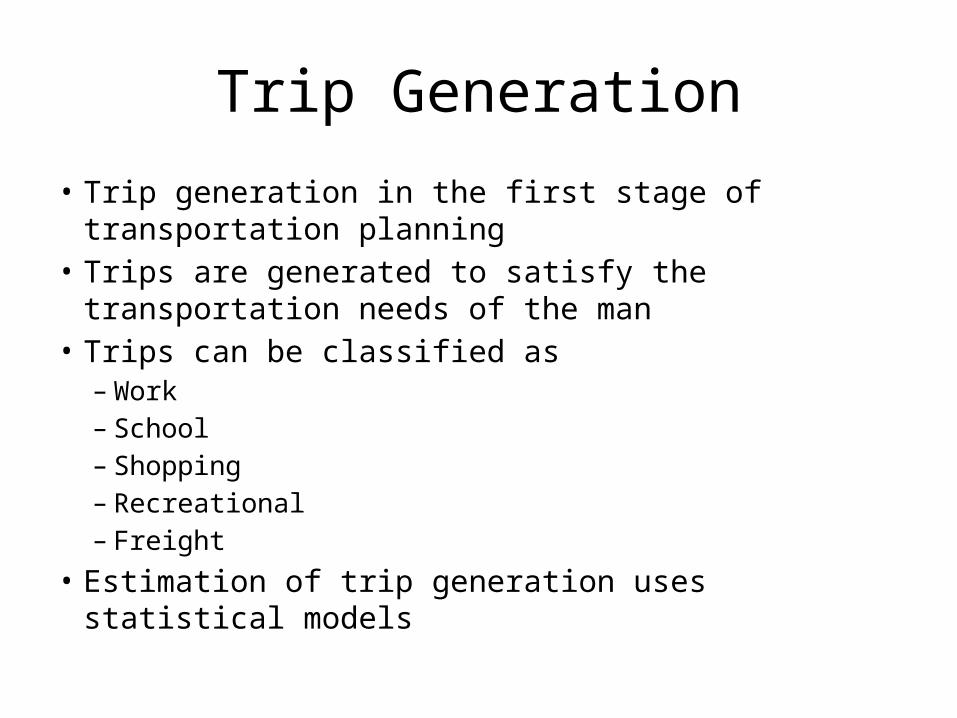
• Trip generation in the first stage of transportation planning• Trips are generated to satisfy the transportation needs of

the man• Trips can be classified as

– Work– School– Shopping– Recreational– Freight

• Estimation of trip generation uses statistical models

Trip Generation

Trip Ends, Productions and Attractions.

ResidentialResidential

Zone jZone i

Nonresidential(business, schools, industry)

Nonresidential(business, schools, industry)

Note : 1. Each zone has two trip ends 2. Zone i has two trip productions 3. Zone j has two trip attractions

Production end

Production end

Attraction end

Attraction end

Urban Zones

• Individual travel patterns are difficult to trace in a region.

• Therefore, a region is divided into easy travel analysis zones of similar travel requirement

• The zones are residential, non residential or mixed (residential and non - residential).

• Residential zones produce trips• Non-residential zones attract trips. • Residential and non - residential zones produce and

attract trips.

Zonal Characteristics (Attributes)

• Zonal population• Average zonal income, • Average vehicle ownership, • Average adults per household• Industries• Commercial activities• Public activities

Households• Zonal averages in a residential zone do not show

variability of the attributes within the zone. • This affects accuracy of estimated trip levels. Eg.

Income levels differ from household to household. • Therefore, households are used as the smallest

entities in modern trip production models. • Zone based models are known as aggregate models • Household based models are known as

disaggregate models.

Trip Purpose Analysis of trips by purpose help more accurate.

Bexause they have similar characteristics of mode of travel and timing.

The main trip purposes are, Work trips School trips Shopping trips Social trips Recreational trips.

Trip generation models

• Estimate the trips generated by a zone using zonal attributes.

• The commonly used statistical models are,

• Regression models• Trip rate analysis models • Cross classification models.

Regression models

• Y = b0 + b1*X1 + b2*X2 + b3*X3 + b4*X4

• Y is the dependent variable ( No of trips generated in a zone)

• X1, X2, X3, X4 etc. are independent variables (Zonal attributes).

• b0, b1, b2, b3, b4 etc. are the model parameters.

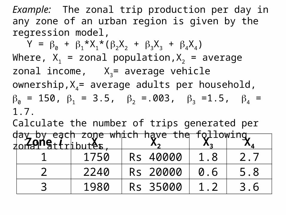
Example: The zonal trip production per day in any zone of an urban region is given by the regression model,

Y = b0 + b1*X1*(b2X2 + b3X3 + b4X4)Where, X1 = zonal population,X2 = average zonal income, X3= average vehicle ownership,X4= average adults per household,b0 = 150, b1 = 3.5, b2 =.003, b3 =1.5, b4 = 1.7.Calculate the number of trips generated per day by each zone which have the following zonal attributes,

Zone i X1 X2 X3 X4

1 1750 Rs 40000 1.8 2.72 2240 Rs 20000 0.6 5.83 1980 Rs 35000 1.2 3.6

Answer.Trips production per day, by Zone 1

=150+ 3.5* 1750* (0.003*40000+1.5*1.8+1.7*2.7) = 118301

by Zone 2=150+ 3.5* 2240* (0.003*20000+1.5*0.6+1.7*5.8) = 131548

by Zone 3=150+ 3.5* 1980* (0.003*35000+1.5*1.2+1.7*3.6) = 127801

Trip Rate Analysis

• The trip rate analysis is simpler than regression models.

• It is a combination of several models that are developed by determining the average trip production or trip attraction rates associated with the important trip generators within the zone.

• An example of these trip generators is the land use.

Trip generation rates grouped by generalized land use categories in downtown . (Ref. Fundamentals of Transportation Engineering by CS Papacostas. p 254)

Land use category Floor space (m2) Person trips Trip Rate (Trips /1000 m2)

Residential 254926 6574 25.8

Commercial - Retail 625423 54833 87.7Commercial - Wholesale 241455 3162 13.1

Commercial - Services 1254748 70014 55.8

Manufacturing 129321 1335 10.32

Transportation 129507 5630 43.47

Public Buildings 276572 11746 42.47

Person trips per hectare by land use and zone. (Ref. Fundamentals of Transportation Engineering by CS Papacostas p 255)

Personal trips per hectare

Zone Residential

Commercial Manufact

uring

Transportation

Publicbuildings

Publicopenspace

Average

Retail Wholesale

Services

Usedland

Allland

1 128 850 135 445 353 73 595 5 128 1002 108 423 90 258 183 25 265 3 75 503 93 563 115 505 83 35 375 10 80 554 75 670 73 385 73 25 245 5 65 435 55 463 60 365 55 13 90 5 43 206 45 485 48 338 53 18 48 3 35 137 38 380 40 328 35 15 10 3 28 8

Weighted Average 60 565 328 78 65 23 115 5 50 23

Example: Four zones of an urban region have the following areas of land use. Calculate the trips produced and attracted by the zones using the previously determined average trip rates.

Land use categoryArea (ha)

Zone 1 Zone 2 Zone 3Residential 2500 150 50Commercial Retail 375 900 150

Wholesale 450 500 200Services 150 250 200

Manufacturing 125 0 2500Transportation 80 250 350Public buildings 230 1500 125Public open space 300 350 100

AnswerFirst calculate the trips generated by land use.

Land use categoryTrip production by land use

Zone 1 Zone 2 Zone 3Residential 150000 9000 3000Commercial Retail 211875 508500 84750

Wholesale 147600 164000 65600Services 11700 19500 15600

Manufacturing 8125 0 162500Transportation 1840 5750 8050Public buildings 26450 172500 14375Public open space 1500 1750 500Total 559090 881000 354375

Now sort out trip productions and attractions by residential and non residential trip generation

Type of tripsPersonal trips

Zone 1 Zone 2 Zone 3

Production 150000 9000 3000

Attractions 409090 872000 351375

Total 559090 881000 354375

There are many ways in which the trip rates can be arranged. The following tables show hypothetical examples of different trip rates that can be developed to determine the number of trips generated.Example of person-trip attraction rates.

Trip purpose

Trips per

house-hold

Trips per employee

University High school OtherNon

retail

Retail

CBD Shop center Other

Home based work - 1.70 1.70 1.70 1.70 - - -

Home based shop - - 2.00 9.00 4.00 - - -Home based school - - - - - 0.90 1.60 1.20

Home based other 0.70 0.60 1.10 4.00 2.30 - - -

Non home based 0.30 0.40 1.00 4.60 2.30 - - -

An example of trip generation rates for residential areas

Residential traffic generator

Morning peak (trips/unit) Afternoon peak (trips/unit)In Out Total In Out Total

Single family residence 0.23 0.58 0.81 0.60 0.40 1.00

Multifamily apartments 0.08 0.49 0.57 0.46 0.23 0.69

An example of trip rates for various commercial activities

Commercial trip generator

Trips per 100 m2 GFA* at peak hour of

operation

Trips per 100 m2 GFA* at afternoon peak street-

hourDrive in restaurants 276.6 116.3Sit down restaurants 37.7 26.9Food stores 15.1 12.9Neighbourhood shopping centres 16.1 15.1

Automobile service stations 30.1 24.8Motels 0.9 0.6Office buildings 2.5 2.5Hospitals 1.1 0.8

*Gross Flow Area (GFA) of buildings

Cross Classification Models• Cross classification is an extension of simple trip rate

analysis• They are zone based models but in trip generation they

are used as disaggregate models. • In residential trip generation, households are further

subdivided into categories or classes that highly correlate with trip making.

• Trip rates associated with each category of households are estimated by statistical methods.

• These rates which are assumed to remain stable over time are used to estimate trip generation in similar zones.

Example of home based non work trip production rates for cross classification

Area typeVehicles

available per household

Trips per household per dayNo of persons per household

1 2-3 4 5+

Urban high density

0 0.57 2.07 4.57 6.951 1.45 3.02 5.52 7.90

2+ 1.82 3.39 5.89 8.27

Suburban medium density

0 0.97 2.54 5.04 7.421 1.92 3.49 5.99 8.37

2+ 2.29 3.86 6.36 8.74

Rural low density

0 0.54 1.94 4.44 96.821 1.32 2.89 5.39 7.77

2+ 1.69 3.26 5.76 8.14

Example: An urban zone contains 200 hectares of residential land, 50 hectares of commercial land and 10 hectares of park land. The zone’s predicted target year household composition is as follows,

Vehicles per

household

Number of householdsNo of persons per household

1 2-3 4 5+

0 100 200 150 201 300 500 210 50

2+ 150 100 60 00Using the calibrated cross classification rates given in previous table, estimate the total home based non work trips that the zone produces during a typical day of the target year.

AnswerThis is a high density zone (large residential area). The total trip productions Pi of the zone i estimated by summing up the contributions of each household type is given by,

h

hhi RNP

where Nh is the number of households type h and Rh is the corresponding trip production rate. Thus, the trip productions by each house hold type is given by,

Vehicles per household

Number of trips generated by household typeTotal by

household type

No of persons per household

1 2-3 4 5+

0 100 x 0.57 200 x 2.07 150 x 4.57 20 x 6.95 12961 300 x 1.45 500 x 3.02 210 x 5.52 50 x 7.90 3499

2+ 150 x 1.82 100 x 3.39 60 x 5.89 00 x 8.27 965Grand Total 5760

An example of procedure for prediction of trip attraction and trip production

Forecast by zone of total households, distribution of household size and vehicle availability

Inputs

Identify area type by zone

Apply trip production rates by zone

Trip production by purpose, by zone and totals by purpose

Trip productionApply trip attraction rates by zone

Obtain total trip attraction by zone and purpose

Compare regional totals to trip production and factors if necessary

Trip attraction by purpose, by zone and totals by purpose

Trip attractionSubtract special attractors from zone totals

Estimate special attractor trip totals by site

Split special attractor trips by purpose by site.

Special attractors

Forecasts by zone of employmant by type, school enrollment, area of parks

Identify special attraction sites

Inputs

Output

Output