trip generation mvs08_chap03

7/28/2019 Trip Generation Mvs08_chap03

http://slidepdf.com/reader/full/trip-generation-mvs08chap03 1/28

CHAPTER 3 – TRIP GENERATION

SCAG 2008 Regional Model

Contents

Introduction ................................................................................................... 3-1Trip Purpose .................................................................................................. 3-1Vehicle Availability Model ........................................................................... 3-2Trip Market Segmentation ....................................................................... 3-11Trip Productions Model ........................................................................... 3-14Trip Attractions Model............................................................................. 3-19Trip Productions Model Validation ....................................................... 3-21



-1


CHAPTER 3 – TRIP GENERATION

Introduction

Trip generation is the process of estimating daily person trips for an average weekday generated byhouseholds within each TAZ. The Year 2008 Model contains a series of models to estimate tripproductions and trip attractions by trip type. The trip production models estimate the number of person trips generated in each TAZ, and trip attraction models estimate the number of person tripattracted to each TAZ. Trip generation estimates trip production and attraction at the Tier 2 zonallevel. The trip generation component includes an Auto Availability model, which forecasts the numberof vehicles available to each household in the region. Auto availability, along with household income,household size, number of workers and other variables are used to forecast trip productions, while tripattractions are a function of land use activity measures such as employment, residential households, andschool enrollment.

Trip Purpose

The model uses an expanded set of trip purposes. This was done to improve trip distribution and modechoice estimates, and to more accurately link trip productions and trip attractions. The model contains10 trip purposes, each subdivided into different household markets. Total trips produced by TAZ wereestimated for each of the following trip purposes and household segments:

1. Home-Based Work

There are two types of home-based work trips: "direct" home-based work trips and "strategic" home-based work trips. "Direct" home-based work (HBWD) trips are trips that go directly between homeand work, without any intermediate stops. "Strategic" home-based work (HBWS) trips are tripsbetween home and work that include one or more intermediate stops, such as to drop-off or pick-up apassenger, to drop-off or pick-up a child at school, or for other reasons. The trip generation modelestimates HBWD and HBWS trips for five household markets, which are carried through tripdistribution and mode choice:

• Zero Car Households

• Car Insufficient Households

• Car Sufficient Households, Low Income (less than $25,000)

• Car Sufficient Households, Medium Income ($25,000 to $49,999)

• Car Sufficient Households, High Income ($50,000 or greater)

2. Home-Based School

Home-based school (HBSC) trips include all student trips with an at-home activity at one end of the tripand a Kindergarten through 12th grade (K-12) school activity at the other end. This purpose does notinclude trips in the college/university category, which follows.

3. Home-Based College and University

Home-based college and university (HBCU) trips include all trips made by persons over the age of 18with an at-home activity at one end of a trip and a college or university activity at the other end.




Page 3-2

4. Home-Based Shopping

Home-based shopping (HBSH) trips include all person trips made with a home activity at one end of atrip and a shopping activity at the other end. The trip generation model estimates HBSH trips for the

same five household markets used for HBW trips. This auto sufficiency / household incomesegmentation is maintained in trip distribution and mode choice. Auto sufficiency is measured differentlyfor work and non-work trips, as described in Table 3-12 below.

5. Home-Based Social-Recreational

Home-based social-recreational (HBSR) trips include all person trips made with a home activity at oneend of a trip and a visiting or recreational activity at the other end. The model estimates HBSR trips forthe five household markets used for HBSH trips, maintained through trip distribution and mode choice.

6. Home-Based Serving-Passenger

Home-based serve passenger (HBSP) trips include all person trips made with a home activity at one endof a trip and a passenger serving activity, such as driving someone to somewhere, at the other end. Tripsthat serve passengers while on the way to work are classified as home based work strategic trips ratherthan serve passenger trips because they are part of a work trip chain. The model estimates HBSP tripsfor the five household markets used for HBSH trips, also maintained through trip distribution and modechoice.

7. Home-Based Other

Home-based other (HBO) trips include all other home-based (with a home activity at one end of a trip)trips that are not already accounted for in any of the home-based trips categories described above. Themodel estimates HBO trips for the five household markets used for HBSH trips, also maintained

through trip distribution and mode choice.

8. Work-Based Other

Work-based other trips are non home-based trips where at least one end of a trip is from/to a work location. An example of such a trip would be, “running an errand during lunch hour” from one’s place of employment.

9. Other-Based Other

Other-based other trips are all other trips that do not begin or end at a trip-maker’s home or place of work.

Vehicle Availability Model

Introduction

The auto availability model predicts the number of households with 0, 1, 2, 3, and 4 or more availablevehicles. The model was estimated in a multinomial logit form using the ALOGIT software. This model isthe first model applied in the model chain. As is customary, the model was estimated using householdrecords, and then applied at the aggregate, TAZ level. The auto availability model includes indicators for




Page 3-3

household size, household income, number of workers, type of housing unit, residential and employmentdensity, and transit and non-motorized accessibilities.

Estimation Dataset

The SCAG 2000 household travel survey final sample consists of 16,939 households. After excludingrecords with unknown or invalid household income, the estimation dataset comprises 14,878 householdrecords. Table 3-1 shows the number of sample households by auto availability and by the fourhousehold attributes included in the estimation file.

Table 3-1: Observed Household Frequencies

Count Percent

Auto Availability

Zero vehicle 1,059 6%One 5,977 35%

Two 6,745 40%Three 2,232 13%Four or more 926 5%Household Size

One person 5,108 30%Two 5,929 35%Three 2,393 14%Four or more 3,509 21%Household Workers

Zero workers 4,055 24%One 7,214 43%Two 4,848 29%Three or more 822 5%

Household Income0 - $25K 3,386 20%$25K- $50K 4,111 24%$50K - $100K 5,215 31%$100K or more 2,166 13%unknown 2,061 12%Type of Housing Unit

Single family detached 10,585 62%Other 6,354 38%

The survey observations were joined with multiple measures of residential density, employment density,and transit and non-motorized accessibility. Table 3-2 shows a complete list and definitions of all the

density and accessibility measures examined during model estimation.




Page 3-4

Table 3-2: Land Use Form and Accessibility Measures

Measure Description and Formulas

Density MeasuresDensity measures are calculated over a 1/2 mile radius of the TAZcentroid. These densities are based on total area, instead of developedarea.

Household Density Total Households / AreaRetail Employment Density Retail Employment / AreaTotal Employment Density Total Employment / Area

Diversity Measures

The indicators of diversity may be proportional to geometric averages of various land uses. These variables take the highest values when all theuses are high and equally allocated. Diversity can also be expressed asthe relative difference between various land uses. The highest diversityoccurs when the two land uses are equal, lowest when one or the otherdominates. These measures are calculated over a one-half mile radius of the TAZ centroid.

Retail Employment (RE) and Household

(HH) Diversity0.001 x RE x HH / (RE + HH)

Retail/Service Employment (RSE) andHousehold (HH) Diversity

0.001 x RSE x HH / (RSE + HH)

Jobs/Housing diversity (SACOG)1- [ABS(b*HH - EMP)/(b*HH + EMP)],where b = regional employment / regional households

Job Mix Diversity1-[ABS(b*RE - NRE) /(B*RE + NRE)],Where NRE is non-retail employment and b = regional non retailemployment / regional retail employment

Design MeasuresThe only available urban design indicator is the number of intersections,calculated using the Tele Atlas street network.

Mix Employment, Household and

Intersection Density

Ln {[Int*(Emp*a) * (HH*b)] /[Int + (Emp*a) + (HH*b)]},where:Int= Number of local intersections in 1/2 mile of centroidEmp= Employment within 1/2 mile of centroid

HH= Households within 1/2 mile of centroida= average Int / average Empb= average Int / average HH

Intersection Density 3-way + 4-way intersections / AreaStreet Density Total street length in 1/2 mile radiusConnectivity Index Proportion of 4-way intersections

Accessibility MeasuresAccessibility variables are proportional to the number of opportunities(such as jobs or retail opportunities) that can be reached by auto, transitor walk means.

Transit Accessibility LogsumWhere Timepq is total transit time including a weight of 2 on all out-of-vehicle time components.

Transit Accessibility to Jobs Employment within x minutes of transit (walk access),where x is a category 0-30mins, 30-60mins etc.

Transit Accessibility to Retail Retail employment within 30 minutes of transit (walk)Transit Stop Density Number of transit stops / Area

Non-Motorized Accessibility




Page 3-5

The mix employment, household and intersection density indicator proved to be the strongest designand density indicator for this region. Figure 3-1 shows how this mix density measure varies over themost urbanized areas in the SCAG region. It is highest in areas that combine high residential,employment and intersection density –Los Angeles CBD, Santa Monica and Wilshire Boulevard, West

Hollywood, Burbank, Glendale, Long Beach, and parts of Santa Ana and Orange.

Figure 3-1: Mixed Employment, Residential and Intersection Density

Utility Structure

The utility of having (a) autos available for a household of type (h) located in zone (z) is given by

All household attributes, listed below, are entered in the utility function as indicator variables; thedensity and accessibility terms are all linear in the parameters. The following variables were examined,proved to be significant in the utility functions, and were selected for the final model:

• Household Size – 1, 2, 3, 4 or more persons• Household Income

o Low income (less than $25,000)o Medium income ($25,000-$50,000)o High income ($50,000-$100,000)o Very high income ($100,000 or more)

• Number of Workers in Household – 0, 1, 2, 3 or more workers




Page 3-6

• Type of Housing Unito Single-Family Detachedo Multi-Family (duplex, apartment, and condominium)

• Transit Accessibility Logsum (LS)

• Mix Household, Employment, and Intersection Density (MixDen)

• Non Motorized Accessibility (WlkAcc)

Estimation Results

Table 3-3 shows the final auto availability model estimation results. All variables show expected, logicalsigns, and most are significant at 95% confidence. Auto availability increases with household size,household income and the number of workers in the household, and decreases for households living inmulti-family housing. Auto availability decreases with increasing transit and walk accessibility toemployment, and also decreases with increasing mix density.

Many of the candidate density and design variables showed logical, statistically significant effects on theirown, but they tended to be correlated with each other. The mix density measure was preferred becauseit responds to changes in residential and employment density, as well as urban form density (asmeasured by the number of intersections).

Table 3-3: Auto Availability Estimation Results

Auto Availability Choice

1 Car 2 Cars 3 Cars 4+ Cars

Coeff. t-stat Coeff. t-stat Coeff. t-stat Coeff. t-stat

Household Income

Low -2.8138 -6.8 -4.7168 -11.3 -5.5354 -12.9 -6.1442 -13.4

Medium -1.3453 -3.2 -2.6003 -6.2 -3.0210 -7.1 -3.6313 -8.3High -0.3288 -0.7 -0.7827 -1.8 -0.9589 -2.1 -1.1941 -2.6

Household Size

2 Person HH 2.0175 33.1 1.9849 18.5 1.4450 8.8

3 Person HH 1.8057 22.6 2.4022 19.7 1.6413 8.94+ Person HH 2.0975 27.8 2.3327 19.5 2.3295 13.6

Workers in HH

1 Worker HH 0.8839 10.5 1.0585 10.9 1.1472 9.2 1.3116 7.1

2 Workers HH 0.4965 3.5 1.5991 10.9 1.8583 11.1 2.1258 9.8

3+ Workers HH 0.7428 4.1 2.7108 14.1 3.7370 15.6Multi-Family Housing -0.3262 -3.9 -1.0705 -11.6 -1.7900 -15.6 -2.1969 -13.2

Mix Emp, Hhld. And Int. Density -0.0494 -2.2 -0.0731 -3.2 -0.1034 -4.3 -0.1181 -4.5

Non Motorized Accessibility -0.3820 -2.0 -0.6870 -2.0Transit Accessibility Logsum -0.0884 -3.9 -0.0853 -3.6 -0.0853 -0.0853

Constant 4.3911 9.9 4.2830 9.6 3.3968 7.4 2.8727 5.9

Notes:

Observations: 14,868

Final log likelihood: 14,940

Rho-Squared (zero): 0.376

Rho-Squared (constants): 0.245




Page 3-7

Model Calibration

The model was first applied to a Year 2000 base scenario and calibrated to match the auto availabilityshares observed in the CTPP 2000 dataset. Subsequently the model was applied to the 2008 base year,with all density measures computed at the Tier 2 zone level. The 2008 model forecast was validated toACS 2005-2009 release data. A comparison of the model forecast to CTPP 2000 and ACS 2005-2009data, for each county in the SCAG region, is shown in Table 3-4 and Table 3-5.

Table 3-4: Year 2000 Auto Availability Forecast - County of Residence Validation

CTPP 2000 Auto Availability

Residence County 0Cars 1Car 2Cars 3Cars 4+Cars Total

Imperial 4,215 13,365 14,355 5,495 2,000 39,430

Los Angeles 391,135 1,154,740 1,084,325 355,510 150,570 3,136,280

Orange 53,695 289,380 400,395 134,615 58,070 936,155Riverside 36,035 174,860 199,405 68,340 28,145 506,785

San Bernardino 41,710 170,245 205,325 78,625 32,935 528,840

Ventura 12,075 67,720 105,805 40,210 17,690 243,500

Total 538,865 1,870,310 2,009,610 682,795 289,410 5,390,990

2000 Model Forecast


Imperial 3,305 15,270 13,811 5,035 1,959 39,380

Los Angeles 398,994 1,139,639 1,090,195 353,769 149,865 3,132,462

Orange 57,848 287,477 397,136 133,240 59,577 935,279

Riverside 33,236 180,446 190,541 72,527 29,468 506,218

San Bernardino 35,491 178,883 207,274 76,055 30,833 528,537

Ventura 11,900 70,027 101,855 40,853 18,596 243,232

Total 540,775 1,871,742 2,000,811 681,481 290,299 5,385,108

Forecast Difference


Imperial (910) 1,905 (544) (460) (41) (50)

Los Angeles 7,859 (15,101) 5,870 (1,741) (705) (3,818)

Orange 4,153 (1,903) (3,259) (1,375) 1,507 (876)

Riverside (2,799) 5,586 (8,864) 4,187 1,323 (567)San Bernardino (6,219) 8,638 1,949 (2,570) (2,102) (303)

Ventura (175) 2,307 (3,950) 643 906 (268)

Total 1,910 1,432 (8,799) (1,314) 889 (5,882)




Page 3-8

Table 3-5: Year 2008 Auto Availability Forecast – County of Residence Validation

ACS 2005-2009 Auto Availability

Residence County 0Cars 1Car 2Cars 3Cars 4+Cars TotalImperial 5,022 14,658 16,371 6,919 3,435 46,405

Los Angeles 300,094 1,105,169 1,123,597 430,792 216,026 3,175,678

Orange 45,379 279,591 407,333 159,368 81,130 972,802

Riverside 29,360 191,759 254,724 112,203 57,038 645,084

San Bernardino 30,030 162,589 224,543 112,044 59,681 588,887

Ventura 10,497 67,105 103,869 49,793 25,876 257,140

Total 420,382 1,820,871 2,130,438 871,119 443,186 5,685,995

2008 Model Forecast


Imperial 6,748 19,223 14,134 6,631 3,264 50,000

Los Angeles 297,797 1,170,600 1,175,672 463,590 273,449 3,381,108

Orange 42,906 308,147 419,677 161,550 100,608 1,032,887

Riverside 40,717 245,517 236,917 108,850 67,435 699,436

San Bernardino 36,317 195,893 213,705 110,543 75,214 631,672

Ventura 11,953 79,085 100,319 51,354 31,586 274,297

Total 436,438 2,018,465 2,160,424 902,517 551,556 6,069,400

Forecast Difference (%), County Normalized


Imperial 2.67% 6.86% -7.01% -1.65% -0.87% 0.0%Los Angeles -0.64% -0.18% -0.61% 0.15% 1.29% 0.0%

Orange -0.51% 1.09% -1.24% -0.74% 1.40% 0.0%

Riverside 1.27% 5.38% -5.61% -1.83% 0.80% 0.0%

San Bernardino 0.65% 3.40% -4.30% -1.53% 1.77% 0.0%

Ventura 0.28% 2.74% -3.82% -0.64% 1.45% 0.0%

Total -0.20% 1.23% -1.87% -0.45% 1.29% 0.0%

An important validation measure is to ascertain whether the model matches the observed pattern of auto availability level by urban form geographies. A comparison of auto availability obtained from ACS

data to the model estimates, classified into density or accessibility bins, shows that the modelreproduces the observed patterns, in the aggregate. Similarly, a comparison of zero car households atthe Regional Statistical Area (RSA) level shows that the model predicts well the number of zero-carhouseholds and the total number of available vehicles. Tables 3-6 to 3-8 and Figures 3-2 and 3-3 providemore information.




Page 3-9

Table 3-6: Auto Availability Validation to Mix Employment, Household and IntersectionDensity

Auto

Availability

Share of Households by Mix Density Level

ACS 2005-2009 Model 2008 Estimate

7 or less 7 to 8.5 8.5 to 9.5 9.5 + 7 or less 7 to 8.5 8.5 to 9.5 9.5 +

0 3% 4% 7% 13% 4% 5% 7% 13%

1 24% 27% 32% 43% 29% 29% 33% 41%

2 42% 40% 37% 32% 37% 39% 37% 31%

3 20% 19% 15% 9% 19% 17% 15% 10%

4+ 10% 10% 8% 4% 12% 10% 9% 6%Total 100% 100% 100% 100% 100% 100% 100% 100%

Table 3-7: Auto Availability Validation to Non Motorized Accessibility

Auto

Availability

Share of Households by Non Motorized Accessibility


6 or less 6 to 8 8 to 10 10 + 6 or less 6 to 8 8 to 10 10 +

0 4% 8% 13% 25% 4% 7% 13% 22%

1 25% 33% 43% 43% 29% 33% 41% 44%

2 41% 37% 32% 26% 37% 36% 30% 23%

3 20% 15% 9% 4% 18% 14% 10% 7%

4+ 10% 8% 4% 2% 11% 9% 6% 4%Total 100% 100% 100% 100% 100% 100% 100% 100%

Table 3-8: Auto Availability Validation to Transit Accessibility Logsum

Auto

Availability

Share of Households by Transit Accessibility Logsum


9 or less9.5 to

1212 to 13.5 13.5 + 9 or less

9.5 to

1212 to 13.5 13.5 +

0 5% 5% 7% 17% 6% 4% 7% 16%1 29% 27% 33% 42% 36% 28% 33% 43%

2 40% 40% 38% 29% 32% 40% 38% 25%

3 18% 19% 15% 8% 16% 17% 14% 10%

4+ 9% 9% 8% 4% 11% 10% 8% 7%

Total 100% 100% 100% 100% 100% 100% 100% 100%




Page 3-10

Figure 3-2: Validation of Zero Car Households for Regional Statistical Areas

Figure 3-3: Validation of Total Auto Availability for Regional Statistical Areas

0

10,00020,000

30,000

40,000

50,000

60,000

70,000

80,000

90,000

100,000

0 10,000 20,000 30,000 40,000 50,000 60,000 70,000 80,000 90,000100,000

2 0 0 8 M o

d e l E s t i m a t e

Observed (ACS 2005-2009)

Zero Car Households

050,000

100,000

150,000

200,000

250,000

300,000

350,000

400,000

450,000

500,000

0 100,000 200,000 300,000 400,000 500,000

2 0 0 8 M o d e l E s t i m a t e

Observed (ACS 2005-2009)

Total Autos

R =0.98

R2

=0.99




Page 3-11

Trip Market Segmentation

Market segmentation is the technique used in trip-based model to subdivide the population into groups

expected to exhibit similar travel behavior. The model segmentation is partly determined by theavailability of survey and census data to identify specific markets or population subgroups and supportthe estimation and validation of separate models for each subgroup.

Trip Purposes

The internal person trip market is stratified into the ten purposes listed in Table 3-9. The external tripmarket is segmented into internal-external (IE/EI) and external-external trips.

Table 3-9: Trip Purposes

Purpose Description

HBWD Home Based Work - Direct

HBWS Home Based Work - StrategicHBCU Home Based College and University

HBSC Home Based School

HBSH Home Based Shop

HBSR Home Based Social and Recreation

HBSP Home Based Serve PassengerHBO Home Based Other

WBO Non Home Based Work

OBO Non Home Based Other

Time Periods

As is customary in a trip-based model, the SCAG model segments the demand models (auto ownership,trip generation, trip distribution, and mode choice) into two time periods - peak and off-peak. The peak periods are 6:00 AM to 9:00 AM in the morning and 3:00 PM to 7:00 PM in the evening. The transitassignments are also performed for these two time periods.

The model uses five periods for highway assignment. The five highway assignment time periods are:

• AM Peak: 6:00 AM to 9:00 AM

• Midday: 9:00 AM to 3:00 PM

• PM Peak: 3:00 PM to 7:00 PM

• Evening: 7:00 PM to 9:00 PM

• Night: 9:00 PM to 6:00 AM

A representative peak period travel time is fed back from the highway assignment to the demand model.This representative time is a weighted average of the AM peak travel time and the PM peak travel time,where the weights equal the proportion of peak period trips that occur in the AM and PM periodsrespectively.




Page 3-12

Household Classifications

In addition to trip purpose and time period, the trip market is further defined by household attributes.The proposed classifications for each model component are summarized in Table 3-10. The groups tobe used for each household classification variable are the following:

• Household Income: low (less than $20,000, medium ($20,000 to $49,999), high ($50,000 to$99,999) and very high (more than $100,000), in $1999.

• Household Size: one, two, three, four or more persons in household.

• Workers in Household: zero, one, two, three or more workers in household.

• Auto Availability: zero, one, two, three, and four or more autos in household.

• Type of Housing Unit: single-family detached unit, all other unit types.

• Age of Head of Household: 18 to 24, 25 to 44, 45 to 64, 65 years old or older.

• Age: number of household members younger than 5, 5 to 17, 18 to 24, 25 years old or older.

Table 3-10: Person and Household Attributes

ModelHhld.

Income

Hhld.

Size

Hhld

Workers

Auto

Availability

Type of

Housing

Unit

Age of

Head of

Hhld.

Age

Auto Ownership X X X X

Trip Production

HBW, WBO X X X X

HBSC, HBCU X

HBO, OBO X X X

Trip Distribution

HBW, WBO X X X

HBO, OBO X X XMode Choice X

HBW, WBO X X X

HBO, OBO X X X

The household income segments were defined to approximately match the household income quintilesused by SCAG in their environmental justice analyses, without significantly deviating from the subgroupsused to report income in the various regional surveys (see Table 3-11). Because of the disparity of income ranges used by the different surveys, it was necessary to impute some of the aggregate incomedata, and/or merge the high and very high income groups in the model estimation work. The specificstrategy used to overcome the survey income disparities is discussed separately for each model

component in the following sections.




Page 3-13

Table 3-11: Survey Household Income Classifications

Annual Household

IncomeHouseholds Quintiles

1999

Census

2001

HIS

2001

MTA

2006

MTA

2010

OCTA

2008

Metrolink

Less than $7,500 481,452 Less than$19,360

X X X X

X X $7,500 to $10,000

X X $10,000 to $14,999 316,692 X

X $15,000 to $19,999 311,115 X X X

$20,000 to $24,999 325,475 $19,361to

$36,340

X X X

$25,000 to $29,999 310,709 X X X X

$30,000 to $34,999 313,862 X

X

X $35,000 to $39,999 290,243

$36,340to

$57,323

X

X X X $40,000 to $44,999 277,669 X X

$45,000 to $49,999 244,079 X

$50,000 to $59,999 455,185 X X

X X

X

X

$60,000 to $74,999 560,767 $57,324to

$91,402

X X

$75,000 to $99,999 601,404 X X X

$100,000 to $149,999 525,328 $91,403or more

X X X X

$150,000 to $200,000342,916 X X X

X

$200,000 or more X

The trip production, destination choice and mode choice models use a market stratification defined byhousehold income and car sufficiency. Car sufficiency is defined relative to household workers for HBWtrips, and relative to household size for HBO trips. The specification of each stratum is shown in Table3-12.

Table 3-12: Trip Market Strata

Trip Market HBW Trips HBO Trips

1 Zero car households, all incomes Zero car households, all incomes

2Households with fewer cars than workers, all

incomes1 car, 2+ person households, all incomes

3Equal or more cars than workers, income less

than $25,0001 car, 1 person households or 2+ car

households, and income less than $25,000

4Equal or more cars than workers, incomeequal or higher than $25,000 and less than

$50,000

1 car, 1 person households or 2+ carhouseholds, and income equal or higher than

$25,000 and less than $50,000

5

Equal or more cars than workers, and income

equal or higher than $50,000

1 car, 1 person households or 2+ car

households, and income equal or higher than$50,000




Page 3-14

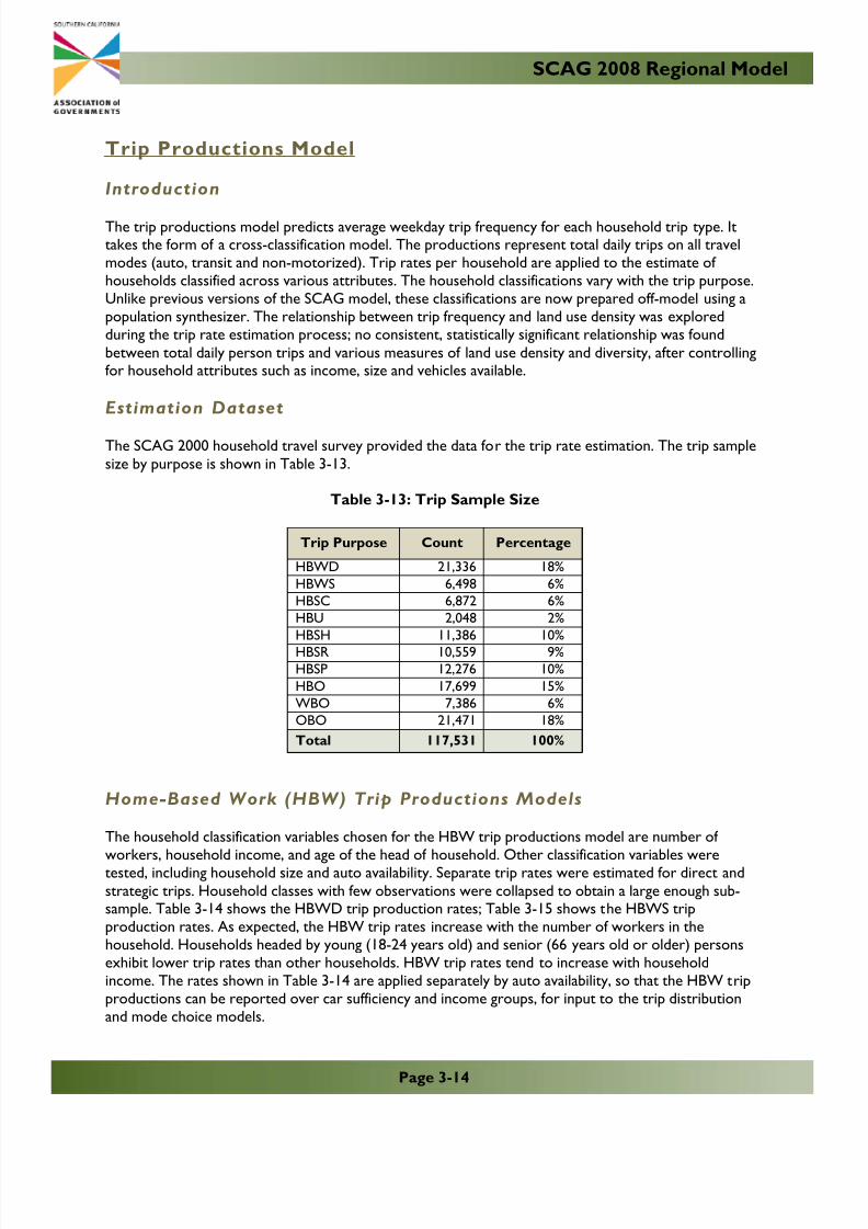
Trip Productions Model

Introduction

The trip productions model predicts average weekday trip frequency for each household trip type. Ittakes the form of a cross-classification model. The productions represent total daily trips on all travelmodes (auto, transit and non-motorized). Trip rates per household are applied to the estimate of households classified across various attributes. The household classifications vary with the trip purpose.Unlike previous versions of the SCAG model, these classifications are now prepared off-model using apopulation synthesizer. The relationship between trip frequency and land use density was exploredduring the trip rate estimation process; no consistent, statistically significant relationship was foundbetween total daily person trips and various measures of land use density and diversity, after controllingfor household attributes such as income, size and vehicles available.

Estimation Dataset

The SCAG 2000 household travel survey provided the data for the trip rate estimation. The trip samplesize by purpose is shown in Table 3-13.

Table 3-13: Trip Sample Size

Trip Purpose Count Percentage

HBWD 21,336 18%

HBWS 6,498 6%

HBSC 6,872 6%

HBU 2,048 2%

HBSH 11,386 10%HBSR 10,559 9%

HBSP 12,276 10%

HBO 17,699 15%

WBO 7,386 6%

OBO 21,471 18%

Total 117,531 100%

Home-Based Work (HBW) Trip Productions Models

The household classification variables chosen for the HBW trip productions model are number of

workers, household income, and age of the head of household. Other classification variables weretested, including household size and auto availability. Separate trip rates were estimated for direct andstrategic trips. Household classes with few observations were collapsed to obtain a large enough sub-sample. Table 3-14 shows the HBWD trip production rates; Table 3-15 shows the HBWS tripproduction rates. As expected, the HBW trip rates increase with the number of workers in thehousehold. Households headed by young (18-24 years old) and senior (66 years old or older) personsexhibit lower trip rates than other households. HBW trip rates tend to increase with householdincome. The rates shown in Table 3-14 are applied separately by auto availability, so that the HBW tripproductions can be reported over car sufficiency and income groups, for input to the trip distributionand mode choice models.




Page 3-15

Table 3-14: HBWD Trip Production Rates

Workers Age of Head of HouseholdHousehold Income ($1999)

<25K 25K-50K 50K-100K >100K

1 18-24 1.098 1.383 1.540 1.4631 25-44 1.164 1.383 1.540 1.463

1 45-65 1.310 1.326 1.428 1.409

1 66+ 0.842 1.260 1.401 1.401

2 18-24 1.986 2.292 2.292 2.2922 25-44 2.101 2.336 2.590 2.720

2 45-65 2.150 2.600 2.710 2.713

2 66+ 2.099 2.304 2.304 2.304

3+ 18-24 3.015 3.015 3.015 3.015

3+ 25-44 3.424 3.458 3.945 3.9453+ 45-65 3.608 3.514 3.749 3.942

3+ 66+ 3.353 3.353 3.655 3.655

Table 3-15: HBWS Trip Production Rates

Workers Age of Head of HouseholdHousehold Income ($1999)

<25K 25K-50K 50K-100K >100K

1 18-24 0.260 0.260 0.260 0.260

1 25-44 0.306 0.426 0.514 0.514

1 45-65 0.369 0.379 0.452 0.468

1 66+ 0.229 0.253 0.348 0.363

2 18-24 0.573 0.788 0.788 0.788

2 25-44 0.696 0.775 1.005 1.005

2 45-65 0.677 0.780 0.922 0.993

2 66+ 0.386 0.386 0.749 0.8663+ 18-24 0.769 0.769 0.769 0.769

3+ 25-44 0.909 0.909 0.940 1.103

3+ 45-65 0.853 0.853 0.918 1.103

3+ 66+ 0.726 0.726 0.726 0.726

Home-Based School (HBSC) and Home-Based College (HBCU) Trip

Productions Models

The HBSC trip productions were estimated based on the number of school-age children in a household.A classification of households by the number of children aged 5 to 17 years old is prepared off-model,

along with all the other household classifications. The HBSC trip rates are shown in Table 3-16.

The HBCU trip productions are estimated based on the number of college-age persons in thehousehold, household income, and the group quarters population. The HBCU trip rates are shown inTable 3-17.




Page 3-16

Table 3-16: HBSC Trip Production Rates

Number of Household Members 5-17 years old Trip Rate

0 0.0381 1.252

2 2.466

3+ 4.028

Table 3-17: HBCU Trip Production Rates

Household Income ($1999)Number of Household Members 17 to 25 years old

0 1 2+

0-25K 0.076 0.357 0.686

25K-50K 0.068 0.266 0.469

50K-100K 0.056 0.246 0.487100K+ 0.032 0.284 0.782

Home-Based Non-Work (HBNW) Trip Productions Models

The household classification variables chosen for the HBNW trip productions model are household size,income and auto availability. Separate trip rates were estimated for HBSH, HBSR, HBSP, and HBO trips.Household classes with few observations were collapsed to obtain a large enough sub-sample. TheHBNW trip production rates are shown in Table 3-18. As expected, the HBNW trip rates increase withhousehold size and with auto availability. The HBNW trip rates do not vary much with householdincome, but the income classification was kept so it is available for trip distribution and mode choice.

Table 3-18: HBNW Trip Production Rates

Auto

Availability

Household

Income

Household

Size

Trip Production Rates

HBSH HBSR HBSP HBO

0

0-25K

1 0.340 0.202 0.059 0.3192 0.664 0.452 0.111 0.5063 0.782 0.606 0.850 0.715

4+ 0.960 0.863 2.489 0.940

25K-50K

1 0.306 0.224 0.033 0.3562 0.616 0.463 0.079 0.506

3 0.735 0.611 0.758 0.7154+ 0.912 0.866 2.388 0.940

50K-100K

1 0.299 0.232 0.009 0.3562 0.604 0.466 0.058 0.5063 0.717 0.599 0.691 0.715

4+ 0.894 0.855 2.313 0.940

100K+

1 0.294 0.241 0.002 0.3562 0.593 0.461 0.052 0.5063 0.699 0.602 0.688 0.716

4+ 0.890 0.868 2.296 0.940




Page 3-17

Auto

Availability

Household

Income

Household

Size


HBSH HBSR HBSP HBO

1

0-25K

1 0.560 0.379 0.501 0.6402 0.888 0.649 0.784 0.924

3 0.995 0.815 1.416 1.4274+ 1.164 1.070 3.009 1.978

25K-50K

1 0.504 0.420 0.279 0.640

2 0.824 0.664 0.558 1.216

3 0.935 0.821 1.263 1.4984+ 1.106 1.075 2.886 2.074

50K-100K

1 0.491 0.436 0.080 0.671

2 0.809 0.668 0.407 1.322

3 0.912 0.805 1.151 1.569

4+ 1.085 1.060 2.796 2.486

100K+

1 0.484 0.452 0.018 0.723

2 0.804 0.686 0.368 1.361

3 0.906 0.814 1.146 1.569

4+ 1.080 1.077 2.776 2.486

2

0-25K

1 0.588 0.442 0.260 0.6402 0.931 0.717 0.714 1.072

3 1.042 0.897 1.333 1.427

4+ 1.214 1.152 2.930 2.036

25K-50K

1 0.529 0.490 0.144 0.640

2 0.863 0.734 0.508 1.1303 0.979 0.904 1.189 1.639

4+ 1.153 1.156 2.810 2.104

50K-100K

1 0.516 0.508 0.041 0.671

2 0.847 0.738 0.371 1.337

3 0.955 0.886 1.083 1.743

4+ 1.130 1.141 2.722 2.616

100K+

1 0.509 0.528 0.009 0.723

2 0.842 0.759 0.335 1.378

3 0.948 0.896 1.079 1.754

4+ 1.125 1.159 2.703 2.741

3+

0-25K

1 0.599 0.533 0.158 0.676

2 0.940 0.819 0.191 1.072

3 1.058 1.007 0.993 1.427

4+ 1.230 1.261 2.629 2.036

25K-50K

1 0.539 0.590 0.088 0.6762 0.871 0.839 0.136 1.130

3 0.994 1.015 0.885 1.639

4+ 1.168 1.266 2.522 2.104

50K-100K

1 0.526 0.611 0.025 0.6762 0.855 0.843 0.099 1.337

3 0.969 0.995 0.807 1.7434+ 1.145 1.249 2.443 2.616

100K+

1 0.518 0.635 0.005 0.723

2 0.850 0.866 0.090 1.378

3 0.962 1.006 0.803 1.754

4+ 1.140 1.269 2.425 2.741




Page 3-18

Non-Home Based (NHB) Trip Productions Models

The household classification variables chosen for the NHB trip productions are income, workers andage of householder for work-based trips; and income, size and auto availability for all other non-homebased trips Table 3-19 and Table 3-20 show the WBO and OBO trip rates, respectively.

Table 3-19: WBO Trip Production Rates

Workers in

Household

Household

Size

Household Income ($1999)

<25K 25K-50K 50K-100K >100K

1

1 0.381 0.715 0.919 1.316

2 0.354 0.665 0.855 1.224

3 0.241 0.453 0.582 0.834

4+ 0.203 0.381 0.489 0.701

2

1

2 0.732 1.072 1.252 1.577

3 0.607 0.889 1.038 1.308

4+ 0.574 0.840 0.982 1.237

3+

1

2

3 0.672 0.998 1.189 1.541

4+ 0.629 0.934 1.112 1.441

Table 3-20: OBO Trip Production Rates


Household

Income

Household

Size

Auto Availability

0 1 2 3+

0-25K

1 0.416 1.297 1.355 1.399

2 0.989 1.870 1.912 1.958

3 1.422 2.317 2.367 2.412

4+ 2.586 3.482 3.513 3.553

25-50K

1 0.453 1.414 1.478 1.525

2 1.049 1.984 2.029 2.078

3 1.499 2.443 2.496 2.543

4+ 2.690 3.622 3.654 3.696

50K-100K

1 0.437 1.364 1.425 1.470

2 1.030 1.948 1.992 2.0393 1.461 2.380 2.431 2.478

4+ 2.656 3.576 3.607 3.649

100K+

1 0.444 1.387 1.449 1.495

2 1.052 1.990 2.035 2.083

3 1.481 2.413 2.465 2.512

4+ 2.687 3.617 3.649 3.691




Page 3-19

Trip Attractions Model

The trip attraction models are linear regression models that estimate attractions for each trip purpose,and then allocate total attractions to car ownership/income markets in proportion to the share of productions by household income in each car ownership market. The models are applied in two steps.First, total attractions for each purpose are calculated using the attraction equations shown in Table 3-21. For HBSH trips, attractions are estimated by applying a trip rate R to the zonal retail employment.The steps for calculating R are as follows:

Step 1: Calculate regionwide resident population to retail employment ratio, R1.Step 2: Calculate the same ratio for each RSA, R2.Step 3: Calculate for each RSA the relative retail service index RSI = R2/R1.Step 4: Range bracket RSI to 0.5 – 1.5.Step 5: Assign this RSI to each TAZ of that RSAStep 6: Apply the equation R = 2.105 + 4.108*RSI to estimate the attraction rate

The trip attraction regression models forecast total attractions by TAZ and by household income forHBW trips, and by TAZ total for all other purposes. An allocation process is applied to segment theseattractions into the household markets used by the trip distribution and mode choice models -- zerocars all income, car insufficient all income, car sufficient low income, car sufficient medium income andcar sufficient high income. This allocation process works as follows:

• The HBW zero car and car insufficient trip attractions are computed as a weighted average of the income group attractions. The weights reflect the share of trips of each income group ineach of these two household markets.

• The HBW car sufficient attractions are set to the corresponding household income segmentattractions.

• Then the HBW attractions are balanced to the trip productions in each market.

• For HBSH, HBSR, HBSP and HBO, total attractions are allocated to household trip markets inproportion to the share of trip productions in the market.

The HBSC and HBCU attraction models are based on school and university enrollment, respectively.The trip attraction rates are shown in Table 3-22. In application, the school productions get allocated toschool attractions within the same school district. This is accomplished by balancing the trips at theschool district level. Similarly, the group quarters population is assigned to a college location, to keepthe model from assigning some of these students to the wrong campus. There are several instances of student dormitories located on a TAZ adjacent to the campus TAZ, so not all of the group quarterspopulation HBCU trips are intra-zonal trips.

Table 3-21: HBSC and HBCU Trip Attraction Rates

Trip PurposeTrip Attraction Rate

(attractions per enrolled student)R2

Home-Based School 1.326 0.84

Home-Based College, non GQ 0.549 0.77

Home-Based College, GQ 1.500 n/a



SCAG 2008 Regional Mode

Page 3-20

Table 3-22: Trip Attraction Model Regression Coefficients

Trip Purpose

H o u s e h

o l d s

T o

t a l E

m p l o y m e n t

R e s i d e n

t i a l

P o p u l a

t i o n

L o w - W

a g e

E m p l o y

m e n t

M e d i u m

- W a g e

E m p l o y

m e n t

H i g h - W

a g e

E m p l o y

m e n t

R e t a i l

I n f o r m a t i o n

P r o

f e s s i o n a l S e r v i c e s

E d u c a t i o n & H e a l t h

S e r v i c e

s

A r t s , E n t e r t a i n m e n t ,

A c c o m m o d a t i o n s

a n d F o o

d S e r v i c e s

O t h e r S e r v i c e s

P u

b l i c

A d m i n i s t r a t i o n

K 1 2 E n r o

l l m e n t

C o l l e g e

E n r o

l l m e n t

HBWD1 Low Inc. 1.181

HBWD2 Med Inc. 1.040

HBWD3 High Inc. 1.040

HBWS1 Low Inc. 0.324

HBWS2 Med Inc. 0.339

HBWS3 High Inc. 0.347

HBCU 0.549

HBSC 1.326

HBO 0.270 0.993 0.544 0.993 0.993 3.439

HBSR 0.367 0.578 0.578 0.578

HBSP 0.388 0.454 0.449 0.453

OBO Attraction 0.508 0.180 4.678 0.698 3.136 3.303

WBO Attraction 0.036 0.202 0.513 1.147

OBO Production 0.538 0.162 4.393 1.118 2.568 3.784

WBO Production 0.137 0.227 0.250 5.743



Page 3-21


Trip Production Model Validation

The model was validated to the expanded SCAG 2000 household travel survey and the NHTS 2008dataset.

The expansion factors of the SCAG 2000 household survey were adjusted to account for two instancesof trip under-reporting. A comparison of trip rates between a GPS-based sample and the diary-basedsample showed that households who completed a diary under-reported home-based trips by 12% andnon-home-based trips by nearly 40%. Furthermore, a comparison of trip rates among households thatcompleted the 2-day diary showed that households assigned to Friday/Saturday or Sunday/Mondaycombinations under-reported their trips on the non-weekend day of their 2-day diary.

Table 3-23 shows a comparison of total trips by purpose for the years 2000 and 2008. As shown, themodel applied with the 2000 inputs generates trips by purpose within 5% of the observed trips, andwithin 1% overall of the total observed trips. When applied to 2008, the model forecasts a 6% increasein total trips, reflecting a 6% increase in home-based work trips, approximately 2% increase in home-based school trips, and between 15% to 20% increase in other trips. The same trip rates were applied in2000 and 2008, therefore the differences in trip generation are due to changes in the socio-economiccomposition of the region’s households, including auto availability.

An additional validation point is provided by the National Household Travel Survey (NHTS). The 2008NHTS estimates total trip productions in the SCAG region at nearly 60.5 million trips, which is close tothe model estimate of 62.0 million trips (see Table 3-23). Note that the NHTS trips have not beenlinked in the same manner as the household survey trips; for this reason the NHTS HBW trips areshown as direct trips only. On the other hand, if trips were linked NHTS would exhibit an even lowershare of non-home-based trips. The NHTS SCAG sample consists of 6,700 households, some of whichdid not report a full day’s worth of travel for all household members-- NHTS accepted householdswhen at least half of its adult members completed the trip diary. The SCAG household survey, incontrast, gathered trip data for over 16,000 households and required that all members report acompleted diary to be accepted as a valid observation. Given these and other methodologicaldifferences, the validation of the 2008 model estimates to NHTS is considered adequate (see Tables 3-23 and 3-24).

Table 3-23: Trip Production Validation to Household Survey, 2000 and 2008

Trip Purpose2001

Household

Survey

2000 Model

Estimate% Diff.

2008 Model

Estimate

2008 to 2000

Change

HBWD 7,951,000 8,245,000 4% 8,964,000 1.09

HBWS 2,496,000 2,575,000 3% 2,738,000 1.06

HBSc 4,605,000 4,755,000 3% 4,852,000 1.02HBU 662,000 667,000 1% 688,000 1.03

HBSh 4,446,000 4,710,000 6% 5,360,000 1.14

HBSR 4,242,000 4,362,000 3% 4,934,000 1.13

HBO 7,598,000 7,965,000 5% 8,939,000 1.12HBSP 6,595,000 6,720,000 2% 7,618,000 1.13

OBO 11,233,000 12,709,000 13% 14,543,000 1.14

WBO 3,248,000 3,433,000 6% 3,524,000 1.03

Total 53,078,000 56,341,000 6% 62,160,000 1.10



Page 3-22


Table 3-24: HBW Trip Production Validation to NHTS 2008

Trip Purpose2008 Model

Estimate 2008 NHTS

HBWD 8,964,000 7,908,000

HBO 35,127,000 36,813,000NHB 18,067,000 15,658,000

Total 62,064,000 60,380,000

The validation of Year 2000 HBW trips by household income level is shown in Table 3-25. Nocomparable Year 2008 data is available to validate the 2008 model estimates.

Table 3-25: HBW Trip Production Validation

Trip Purpose and

Household Income

2001 Household

Survey

2000 Model

Estimate% Difference

HBWD 0-25K 950,780 980,934 3%

HBWD 25-50K 2,024,579 2,077,394 3%

HBWD 50-100K 3,086,696 3,342,825 8%

HBWD over 100 K 1,889,752 1,869,919 -1%

HBWS 0-25K 267,693 273,565 2%

HBWS 25-50K 556,251 608,686 9%

HBWS 50-100K 1,023,915 1,076,878 5%

HBWS over 100K 649,042 623,449 -4%

Tables 3-26 and 3-27 provide summary statistics for person trips, by county and for the SCAG region.Table 3-26 shows the share of trips by county and purpose, compared to the 2008 household survey.Table 3-27 identifies selected comparative statistics, such as trips per household, trips per vehicle, andtrips per capita (resident person).



Page 3-23


Table 3-26: Year 2008 Trip Generation Summary by Trip Purpose and by County

TripPurpose

Person Trip Productions

ImperialLos

AngelesOrange Riverside

San

BernardinoVentura

Model

Area Total

HBWD NoCars

1,525 104,225 19,104 5,908 7,744 3,546 142,053

HBWD CarCompetition

8,229 701,643 225,525 82,579 76,300 44,901 1,139,178

HBWD CarSuf. 0-25K

8,807 502,192 139,909 74,080 81,629 29,643 836,260

HBWD CarSuf. 25-50K

14,055 1,082,396 310,261 190,094 215,160 74,397 1,886,363

HBWD CarSuf. over 50K

23,499 2,601,126 1,039,312 495,089 517,598 283,207 4,959,830

HBWS NoCars

481.0586 29,311 5,365 1,614 2,075 981.8732 39,828

HBWS CarCompetition

2,628 197,562 64,234 23,920 21,236 12,961 322,539

HBWS CarSuf. 0-25K

2,798 140,504 39,228 21,383 22,634 8,510 235,057

HBWS CarSuf. 25-50K

4,467 312,070 89,737 57,651 62,345 21,991 548,261

HBWS CarSuf. over 50K

8,355 825,520 335,981 166,803 163,046 92,339 1,592,044

Total Home

Based Work 74,845 6,496,549 2,268,655 1,119,120 1,169,768 572,476 11,701,413

HBSC 50,335 2,640,303 764,232 575,933 602,315 218,587 4,851,705HBCU 5,208 393,249 116,703 72,040 72,418 28,114 687,732

HBSH 45,764 2,938,417 916,603 629,609 583,684 245,468 5,359,545HBSR 32,644 2,700,173 854,227 572,722 546,212 228,435 4,934,414

HBSP 71,460 4,145,896 1,268,159 909,989 888,091 334,645 7,618,240

HBO 56,880 4,848,026 1,578,344 1,044,550 990,877 419,856 8,938,534

Total Home

Based Non

Work

262,291 17,666,064 5,498,269 3,804,844 3,683,597 1,475,106 32,390,170

WBO 19,677 2,036,727 727,957 295,030 298,288 146,744 3,524,422

OBO 108,913 8,024,250 2,846,199 1,487,903 1,426,096 649,672 14,543,033

Total Non-

HomeBased

128,590 10,060,978 3,574,156 1,782,933 1,724,384 796,416 18,067,456

Total

Person

Trips

465,726 34,223,590 11,341,079 6,706,897 6,577,749 2,843,998 62,159,039



Page 3-24


Table 3-27: Year 2008 Trip Generation Comparative Statistics

Home Based

Work Trips Imperial

Los

Angeles Orange Riverside

San

Bernardino Ventura

Model Area

Total

Trips 74,845 6,496,549 2,268,655 1,119,120 1,169,768 572,476 11,701,413

Trips perHousehold

1.54 2.01 2.30 1.65 1.93 2.16 2.01

Trips per Vehicle 0.97 1.15 1.18 0.90 0.99 1.08 1.10

Trips perWorker

1.43 1.59 1.57 1.55 1.61 1.55 1.58

% Home BasedWork Trips

16.1% 19.0% 20.0% 16.7% 17.8% 20.1% 18.8%

Home Based

Non Work

Trips

ImperialLos

Angeles

Orange RiversideSan

Bernardino

VenturaModel Area

Total

Trips 262,291 17,666,064 5,498,269 3,804,844 3,683,597 1,475,106 32,390,170

Trips perHousehold

5.40 5.48 5.57 5.61 6.08 5.56 5.57

Trips per Vehicle 3.40 3.13 2.87 3.05 3.12 2.79 3.06

Trips per Person 1.54 1.81 1.84 1.79 1.83 1.81 1.81

% Home BasedNon Work Trips

56.3% 51.6% 48.5% 56.7% 56.0% 51.9% 52.1%



Page 3-25


Table 3-27: Year 2008 Trip Generation Comparative Statistics (continued)

Non Home

Based TripsImperial

Los

AngelesOrange Riverside

San

BernardinoVentura

Model

Area Total

Trips 128,590 10,060,978 3,574,156 1,782,933 1,724,384 796,416 18,067,456

Trips perHousehold

2.65 3.12 3.62 2.63 2.85 3.00 3.11

Trips perVehicle

1.67 1.78 1.87 1.43 1.46 1.51 1.70

Trips perPerson

0.76 1.03 1.20 0.84 0.86 0.98 1.01

% Home BasedNon Work Trips

27.6% 29.4% 31.5% 26.6% 26.2% 28.0% 29.1%

Total Trips Imperial

Los

Angeles Orange Riverside

San

Bernardino Ventura

Model

Area Total

Trips 465,726 34,223,590 11,341,079 6,706,897 6,577,749 2,843,998 62,159,039

Trips perHousehold

9.58 10.61 11.49 9.88 10.86 10.71 10.69

Trips perVehicle

6.03 6.05 5.92 5.38 5.57 5.38 5.86

Trips perPerson

2.74 3.50 3.79 3.15 3.26 3.50 3.47




THIS PAGE LEFT INTENTIONALLY BLANK

trip generation mvs08_chap03

Documents