Transition Within a Hypervelocity Boundary Layer on

a 5-Degree Half-Angle Cone in Air/CO2 Mixtures

Joseph S. Jewell∗

California Institute of Technology, Pasadena, CA, 91125

Ross M. Wagnild†

Sandia National Laboratories, Albuquerque, NM, 87185

Ivett A. Leyva‡

Air Force Research Laboratory, Edwards AFB, CA, 93536

Graham V. Candler§

University of Minnesota, Minneapolis, MN, 55455

Joseph E. Shepherd¶

California Institute of Technology, Pasadena, CA, 91125

Laminar to turbulent transition on a smooth 5-degree half angle cone at zero angle ofattack is investigated computationally and experimentally in hypervelocity flows of air,carbon dioxide, and a mixture of 50% air and carbon dioxide by mass. Transition N factorsabove 10 are observed for air flows. At comparable reservoir enthalpy and pressure, flowscontaining carbon dioxide are found to transition up to 30% further downstream on the conethan flows in pure air in terms of x-displacement, and up to 38% and 140%, respectively,in terms of the Reynolds numbers calculated at edge and reference conditions.

Nomenclature

f frequencyh enthalpyM Mach numberP pressurePr Prandtl numberR specific gas constantT temperatureu velocityw mass fractionx displacement from the tipγ ratio of specific heatsδ boundary layer thicknessΘ characteristic vibrational temperatureμ dynamic viscosityρ densityτ vibrational relaxation time

∗Ph.D. Candidate, GALCIT, MC 205-45, Caltech. AIAA Student Member.†Senior Member, Technical Staff, Sandia National Laboratories. AIAA Member.‡Sr. Aerospace Engineer, Air Force Research Laboratory. AIAA Associate Fellow.§Professor, University of Minnesota. AIAA Fellow.¶Professor, GALCIT, MC 105-50, Caltech. AIAA Senior Member.

1 of 13

American Institute of Aeronautics and Astronautics

Subscripte condition at the boundary layer edgeres condition in the reservoirtr condition at the location of transitionw condition at the wall

Superscript∗ condition at Dorrance reference temperature

I. Introduction

In hypervelocity flow over cold, slender bodies, the most significant instability mechanism is the so-calledsecond or Mack mode. These flows are characteristic of high-enthalpy facilities like the T5 shock tunnel

at Caltech. A second mode disturbance depends on the amplification of acoustic waves trapped in theboundary layer, as described by Mack.1 Another potential disturbance is the first mode, which is the highspeed equivalent of the viscous Tollmien–Schlichting instability.2 However, at high Mach number (> 4) andfor cold walls, the first mode is damped and higher modes are amplified, so that the second mode would beexpected to be the only mechanism of linear instability leading to transition for a slender cone at zero angleof attack.

Parametric studies in air and CO2 in the T5 hypervelocity reflected shock tunnel by Germain3 andAdam4 on a smooth 5-degree half angle cones at zero angle of attack showed an increase in the referenceReynolds number Re* (see Equation 6 on page 8) at the point of transition as reservoir enthalpy hres in-creased. Germain and Adam also observed that flows of CO2 transitioned at higher values of Re* than flowsof air for the same hres and Pres. Johnson et al.5 studied this effect with a linear stability analysis focused onthe chemical composition of the flow, and found an increase in transition Reynolds number with freestreamtotal enthalpy, and further found the increase to be greater for gases with lower dissociation energies andmultiple vibrational modes, such as CO2. In fact, with the assumption of a transition N factor of 10 thatwas made at the time, none of the CO2 cases computed by Johnson et al. predicted transition at all. Theseeffects led Fujii and Hornung6 to further investigate their hypothesis that the delay in transition was due tothe damping of acoustic disturbances in non-equilibrium relaxing gases by vibrational absorption. Fujii andHornung estimated the most strongly amplified frequencies for representative T5 conditions and found thatthese agreed well with the frequencies most effectively damped by non-equilibrium CO2. This suggests thatthe suppression of the second mode through the absorption of energy from acoustic disturbances throughvibrational relaxation is the dominant effect in delaying transition for high-enthalpy carbon dioxide flows.

Numerous studies have been made on inhibiting the second mode, and therefore preventing or delayingtransition through the suppression of acoustic disturbances within the boundary layer; see Fedorov et al.7 andRasheed8 for work focused on absorbing acoustic energy using porous walls. Another approach to suppressionof the pressure waves that lead to transition centers around altering the chemical composition within theboundary layer to include species capable of absorbing acoustic energy at the appropriate frequencies. Effortsin this area to date have included preliminary experimental work on mixed freestream flows, e.g. Leyva etal.,9 computations, e.g. Wagnild et al.,10, 11 and experiments with direct injection of absorptive gases intothe boundary layer, e.g. Jewell et al.12 The present aim is to confirm and extend these studies bothcomputationally and experimentally by considering transition within a hypervelocity boundary layer on a5-degree half-angle cone in freestream mixtures of air and carbon dioxide.

II. Background

By assuming that the boundary layer acts as an acoustic waveguide for disturbances (see Fedorov13 for aschematic illustration of this effect), the frequency of the most strongly-amplified second-mode disturbancesin the boundary layer may be estimated as Equation (1), as shown in Stetson.14

f ≈ 0.8ue

2δ(1)

Here δ is the boundary layer thickness and ue is the velocity at the boundary layer edge. For a typicalT5 condition in air, with enthalpy of 10 MJ/kg and reservoir pressure of 50 MPa, the boundary layerthickness is on the order of 1.5 mm and the edge velocity is 4000 m/s. This indicates that the most

2 of 13

American Institute of Aeronautics and Astronautics

strongly amplified frequencies are in the 1 MHz range. This is broadly consistent with the results of Fujiiand Hornung.6 Kinsler et al.15 provide a good general description of the mechanisms of attenuation ofsound waves in fluids due to molecular exchanges of energy within the medium. The relevant exchange ofenergy for carbon dioxide in the boundary layer of a thin cone at T5-like conditions is the conversion ofmolecular kinetic energy (e.g. from compression due to acoustic waves) into internal vibrational energy. Inreal gases, molecular vibrational relaxation is a non-equilibrium process, and therefore irreversible. Thisabsorption process has a characteristic relaxation time. The problem of sound propagation, absorption,and dispersion in a dissociating gas has been treated from slightly different perspectives by Clarke andMcChesney,16 Zeldovich and Raizer,17 and Kinsler et al.15 However, in non-equilibrium flows when theacoustic characteristic time scale and relaxation time scale are similar, some finite time is required formolecular collisions to achieve a new density under an acoustic pressure disturbance. This results in a limitcycle, as the density changes lag the pressure changes. The area encompassed by the limit cycle’s trajectoryis related to energy absorbed by relaxation. Energy absorbed in this way is transformed into heat anddoes not contribute to the growth of acoustic waves.9 Carbon dioxide, a linear molecule, has four normalvibrational modes. The first two, which correspond to transverse bending, are equal to each other, and havecharacteristic vibrational temperatures Θ1 = Θ2 = 959.66 K. The third mode, corresponding to symmetriclongitudinal stretching, has Θ3 = 1918.7 K, and the fourth mode, corresponding to asymmetric longitudinalstretching, has Θ4 = 3382.1 K. Camac18 showed that the four vibrational modes for carbon dioxide all relaxat the same rate, and proposed a simplified formula, Equation (2), to calculate vibrational relaxation time,which was reproduced in Fujii and Hornung.6

ln (A4τCO2P ) = A5T−1/3 (2)

Here A4 and A5 are constants given by Camac for carbon dioxide as A4 = 4.8488×102 Pa−1s−1 andA5 = 36.5 K1/3. Using the constants suggested by Camac, with P = 35kPa and T = 1500 K, which areconsistent with a typical T5 condition with enthalpy 10 MJ/kg and stagnation pressure 50 MPa, we findvibrational relaxation time = 1.43×10−6 s, which indicates that frequencies around 700 KHz should be moststrongly absorbed at these conditions. This is, again, broadly similar to the results of Fujii and Hornung,6

who computed curves at 1000 K and 2000 K with peaks bracketing 700 kHz.Thus, in a flow of gas that absorbs energy most efficiently at frequencies similar to the most strongly

amplified frequencies implied by the geometry of the boundary layer, laminar to turbulent transition isexpected to be delayed. Using computations, we show that the flow of carbon dioxide/air mixtures over aslender cone at T5 conditions allows for such a match in frequencies. We then perform a series of experimentsto confirm this effect.

III. Experimental Model

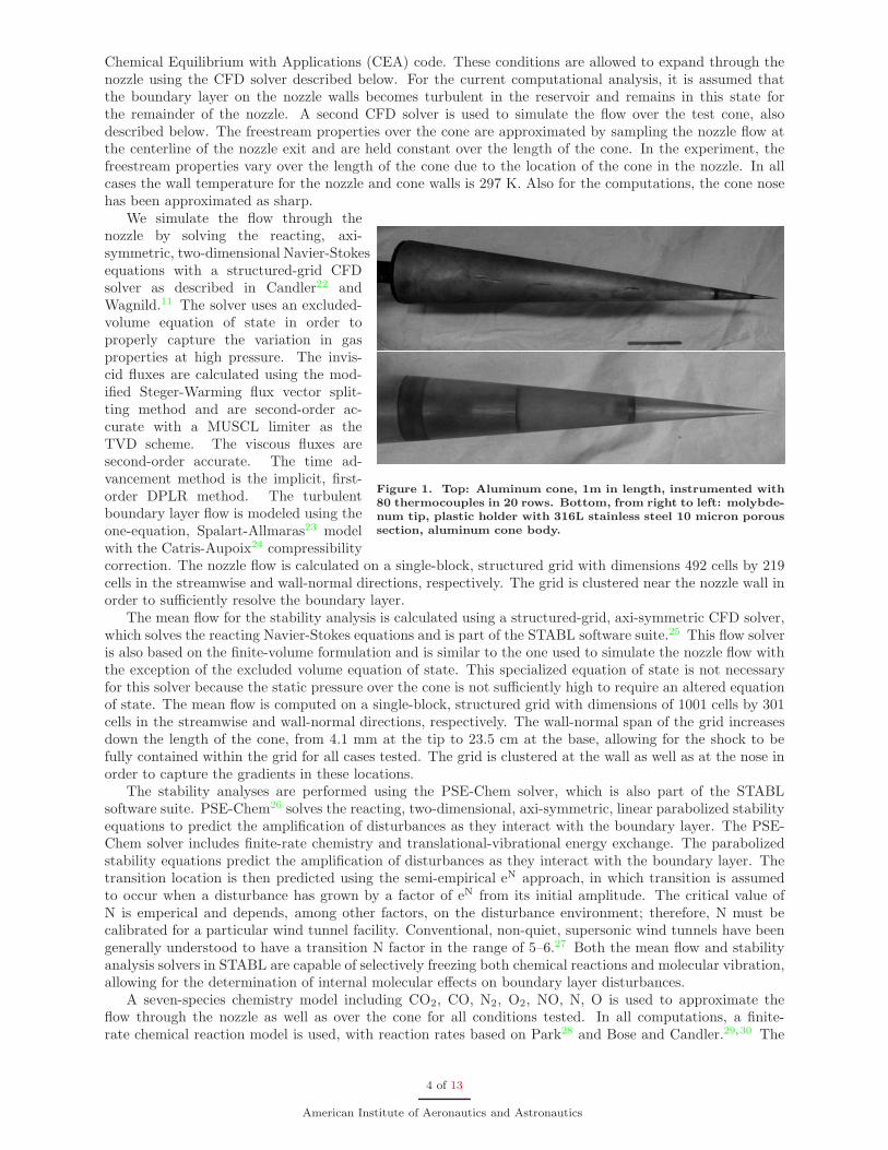
The facility used in all experiments for the current study is the T5 hypervelocity reflected shock tunnel;see Hornung19 and Hornung and Belanger.20 The model is a smooth 5-degree half-angle aluminum conesimilar to that used in a number of previous experimental studies in T5, 1 m in length, and is composedof three sections: a sharp tip (radius ∼0.2 mm) fabricated of molybdenum, an interchangeable mid-sectionwhich may contain a porous gas-injector section (in the present experiments this section is a smooth, solidpiece of plastic), and the main body, which is instrumented with a total of 80 thermocouples evenly spacedat 20 lengthwise locations beginning at 221 mm from the tip of the cone, with each row located 38 mm fromthe last. These thermocouples have a response time on the order of a few microseconds21 and have beensuccessfully used for boundary layer transition determination in Adam and Hornung4 and Rasheed et al.8

The conical model geometry was chosen because of the wealth of experimental and numerical data availablewith which to compare the results from this program. Two photographs of the cone model are shown inFigure 1. The model is mounted such that the tip of the cone protrudes about 380 mm into the T5 nozzleat run time, in order to maximize the linear extent of the cone within the test rhombus defined by theexpansion fan radiating from the nozzle’s edge.

IV. Computational Model

In order to obtain the flow properties over the test cone, we start with the flow properties in the tunnelreservoir, which serves as the inflow for the nozzle flow simulations. The reservoir conditions are obtainedby solving for chemical and thermal equilibrium at the specified reservoir pressure and enthalpy using the

3 of 13

American Institute of Aeronautics and Astronautics

Chemical Equilibrium with Applications (CEA) code. These conditions are allowed to expand through thenozzle using the CFD solver described below. For the current computational analysis, it is assumed thatthe boundary layer on the nozzle walls becomes turbulent in the reservoir and remains in this state forthe remainder of the nozzle. A second CFD solver is used to simulate the flow over the test cone, alsodescribed below. The freestream properties over the cone are approximated by sampling the nozzle flow atthe centerline of the nozzle exit and are held constant over the length of the cone. In the experiment, thefreestream properties vary over the length of the cone due to the location of the cone in the nozzle. In allcases the wall temperature for the nozzle and cone walls is 297 K. Also for the computations, the cone nosehas been approximated as sharp.

Figure 1. Top: Aluminum cone, 1m in length, instrumented with80 thermocouples in 20 rows. Bottom, from right to left: molybde-num tip, plastic holder with 316L stainless steel 10 micron poroussection, aluminum cone body.

We simulate the flow through thenozzle by solving the reacting, axi-symmetric, two-dimensional Navier-Stokesequations with a structured-grid CFDsolver as described in Candler22 andWagnild.11 The solver uses an excluded-volume equation of state in order toproperly capture the variation in gasproperties at high pressure. The invis-cid fluxes are calculated using the mod-ified Steger-Warming flux vector split-ting method and are second-order ac-curate with a MUSCL limiter as theTVD scheme. The viscous fluxes aresecond-order accurate. The time ad-vancement method is the implicit, first-order DPLR method. The turbulentboundary layer flow is modeled using theone-equation, Spalart-Allmaras23 modelwith the Catris-Aupoix24 compressibilitycorrection. The nozzle flow is calculated on a single-block, structured grid with dimensions 492 cells by 219cells in the streamwise and wall-normal directions, respectively. The grid is clustered near the nozzle wall inorder to sufficiently resolve the boundary layer.

The mean flow for the stability analysis is calculated using a structured-grid, axi-symmetric CFD solver,which solves the reacting Navier-Stokes equations and is part of the STABL software suite.25 This flow solveris also based on the finite-volume formulation and is similar to the one used to simulate the nozzle flow withthe exception of the excluded volume equation of state. This specialized equation of state is not necessaryfor this solver because the static pressure over the cone is not sufficiently high to require an altered equationof state. The mean flow is computed on a single-block, structured grid with dimensions of 1001 cells by 301cells in the streamwise and wall-normal directions, respectively. The wall-normal span of the grid increasesdown the length of the cone, from 4.1 mm at the tip to 23.5 cm at the base, allowing for the shock to befully contained within the grid for all cases tested. The grid is clustered at the wall as well as at the nose inorder to capture the gradients in these locations.

The stability analyses are performed using the PSE-Chem solver, which is also part of the STABLsoftware suite. PSE-Chem26 solves the reacting, two-dimensional, axi-symmetric, linear parabolized stabilityequations to predict the amplification of disturbances as they interact with the boundary layer. The PSE-Chem solver includes finite-rate chemistry and translational-vibrational energy exchange. The parabolizedstability equations predict the amplification of disturbances as they interact with the boundary layer. Thetransition location is then predicted using the semi-empirical eN approach, in which transition is assumedto occur when a disturbance has grown by a factor of eN from its initial amplitude. The critical value ofN is emperical and depends, among other factors, on the disturbance environment; therefore, N must becalibrated for a particular wind tunnel facility. Conventional, non-quiet, supersonic wind tunnels have beengenerally understood to have a transition N factor in the range of 5–6.27 Both the mean flow and stabilityanalysis solvers in STABL are capable of selectively freezing both chemical reactions and molecular vibration,allowing for the determination of internal molecular effects on boundary layer disturbances.

A seven-species chemistry model including CO2, CO, N2, O2, NO, N, O is used to approximate theflow through the nozzle as well as over the cone for all conditions tested. In all computations, a finite-rate chemical reaction model is used, with reaction rates based on Park28 and Bose and Candler.29, 30 The

4 of 13

American Institute of Aeronautics and Astronautics

equilibrium coefficients are calculated from fits based on Park31 and McBride et al.32 It is assumed thatthe vibrational-vibrational energy exchanges occur on a relatively short time scale, allowing for a singletemperature governing all vibrational modes. It is also assumed that rotation and translation are coupledand governed by the translational temperature. The translational-vibrational energy exchanges are governedby the Landau-Teller model for the simple harmonic oscillator. The vibrational relaxation times are governedby the Millikan and White model with several empirical corrections given in Camac18 and Park.28 Theviscosity for each species is calculated using Blottner fits and the mixture quantities are calculated usingWilke’s semi-empirical mixing law.

V. Computational Predictions

Mass Fraction CO2

x tr (

m)

0 0.2 0.4 0.6 0.8 10.2

0.4

0.6

0.8

1

10 MJ/kg - 50 MPa8.5 MJ/kg - 45 MPa7 MJ/kg - 40 MPa5 MJ/kg - 30 MPa

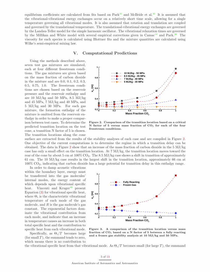
Figure 2. Comparison of the transition location based on a criticalN factor of 5 versus mass fraction of CO2 for each of the fourfreestream conditions.

Using the methods described above,seven test gas mixtures are simulated,each at four different freestream condi-tions. The gas mixtures are given basedon the mass fraction of carbon dioxidein the mixture and are 0.0, 0.1, 0.2, 0.3,0.5, 0.75, 1.0. The freestream condi-tions are chosen based on the reservoirpressure and the reservoir enthalpy andare 10 MJ/kg and 50 MPa, 8.5 MJ/kgand 45 MPa, 7 MJ/kg and 40 MPa, and5 MJ/kg and 30 MPa. For each gasmixture, the formation enthalpy of themixture is omitted from the reservoir en-thalpy in order to make a proper compar-ison between test cases. To determine thepredicted transition location on the testcone, a transition N factor of 5 is chosen.The transition locations along the conesurface are extracted from the results of the stability analyses of each case and are compiled in Figure 2.One objective of the current computations is to determine the regime in which a transition delay can beobtained. The data in Figure 2 show that an increase of the mass fraction of carbon dioxide in the 5 MJ/kgcase has only a small effect on the transition location. At 7 MJ/kg, the transition location moves toward therear of the cone by about 5 cm at 100% CO2. The 8.5 MJ/kg case shows a shift in transition of approximately61 cm. The 10 MJ/kg case results in the largest shift in the transition location, approximately 66 cm at100% CO2, indicating that carbon dioxide has a large potential for transition delay in this enthalpy range.

Mass Fraction CO2

x tr (

m)

0 0.2 0.4 0.6 0.8 1

0.2

0.4

0.6

0.8

1

Fully ReactingFrozen Gas

Figure 3. A comparison of the transition location versus massfraction of CO2 based on a N factor of 5 between a fully reactingand a frozen gas stability analysis at 10 MJ/kg and 50 MPa.

In order to damp acoustic vibrationswithin the boundary layer, energy mustbe transferred into the gas molecules’internal modes, the energy content ofwhich depends upon vibrational specificheat. Vincenti and Kruger33 presentEquation (3) for vibrational specific heat,where Θi is the characteristic vibrationaltemperature of each mode of the gasmolecule, and R is the gas molecule’s gasconstant. The exponential factors dom-inate the vibrational contribution fromeach mode, and indicate that an increasein temperature causes an increase in bothtotal specific heat and the contribution tospecific heat from each vibrational mode.

Specifically, as Θi/T becomes large(for small T ), the summand tends to zero,which means there is no contribution tothe vibrational specific heat from that vibrational mode. As Θi/T becomes small (for large T ), the summand

5 of 13

American Institute of Aeronautics and Astronautics

tends to unity, and the maximum contribution from a given vibrational mode is therefore R. As temperatureincreases within the boundary layer, each mode becomes more fully excited and capable of exchanging moreenergy from acoustic vibrations. Temperature tends to increase with enthalpy. Table 1 on page 8 recordsreservoir enthalpy and T ∗, a characteristic boundary layer reference temperature, for each experiment.

Cvvib= R

∑i

{(Θi

T

)2eΘi/T(

eΘi/T − 1)2

}(3)

Using the ability of the stability analysis in STABL to freeze the chemical and vibrational rate processes,we can determine the effect of these rate processes on the damping of second mode disturbances. An exampleof this type of calculation is demonstrated by comparing the transition location for a fully reacting stabilityanalysis and a frozen gas stability analysis for the 10 MJ/kg case, as shown in Figure 3. Using a reacting meanflow and a frozen gas stability analysis, the data show that adding carbon dioxide promotes transition. Whenthe chemical and vibrational rate processes are included in the stability analysis, the transition location movesfurther down the cone due to carbon dioxide’s ability to damp boundary layer disturbances. By calculatingthe change in transition location, we can compare the effectiveness of disturbance damping in each of thefour freestream conditions, shown in Figure 4. For all cases tested, the addition of chemical and vibrationalrate processes results in a shift in the transition location towards the rear of the cone that increases withan increasing mass fraction of carbon dioxide in the test gas. From these data, it becomes clear that thedamping ability of carbon dioxide is most effective for the 10 MJ/kg case, for the reasons described above.Interestingly, the addition of carbon dioxide in the 5 MJ/kg case has little or no effect as indicated inFigure 2, despite the disturbance damping ability of molecular vibration demonstrated in Figure 4. In thiscase, the optimum disturbance damping frequency of carbon dioxide is no longer similar to the boundarylayer disturbance frequencies.

Mass Fraction CO2

x tr (

m)

0 0.2 0.4 0.6 0.8 1

0.2

0.4

0.6

0.8

10 MJ/kg - 50 MPa8.5 MJ/kg - 45 MPa7 MJ/kg - 40 MPa5 MJ/kg - 30 MPa

Figure 4. Comparsion of the change in transition location due to vibrational relaxation versus mass fractionof CO2 based on a transition N factor of 5 for each of the three freestream conditions tested.

It is also noted that the relatively small effect of vibrational damping shown in Wagnild et al.34 is dueto the total enthalpy of the flow considered in their study, approximately 4.5 MJ/kg. As demonstrated inFigure 4, the vibrational damping of carbon dioxide causes a smaller change in transition location with adecreasing flow enthalpy. Thus, a small change in amplification at 4.5 MJ/kg is expected.

VI. Experimental Results

Although there have been several previous experimental campaigns on transition in T5 (Germain,3 Adamand Hornung,4 Leyva et al.,9 Jewell et al.12), based on recent experience with T5 operations, it is desirableto conduct new experiments with special attention paid to repeatability and cleanliness of the tunnel. Basedon the computations described above, we choose three carbon dioxide/air gas mixtures which were testedin T5 on the 5-degree half-angle cone, with reservoir enthalpies varying from 7.68–9.65 MJ/kg and reservoirpressures held as consistently as possible near 58 MPa, but varying from 53.4–60.7 MPa, to attempt toreproduce the largest shift in transition location implied by the computations. The gas mixtures, by massfraction of carbon dioxide in the mixture, are 0.0 (e.g. all air), 0.5, 1.0. A summary of run conditions andresults is presented in Table 1 on page 8. For the 0.5 mass fraction case, the CO2 and air are not premixed.

6 of 13

American Institute of Aeronautics and Astronautics

The shock tube is filled sequentially and the gases allowed to diffuse into each other for approximately 15minutes before each experiment.

0.2 0.3 0.4 0.5 0.6 0.8 1x−position [m]

106

107

10−4

10−3

10−2

Reynolds number (Rex) [−]

Sta

nto

n n

um

ber

(S

t) [

−]

Plot of St vs Rex for T5−2744; P

res = 60.7 MPa, h

res = 7.68 MJ/kg, T

res = 5250 K

laminarVan Driest IIWhite & Christophexperimental

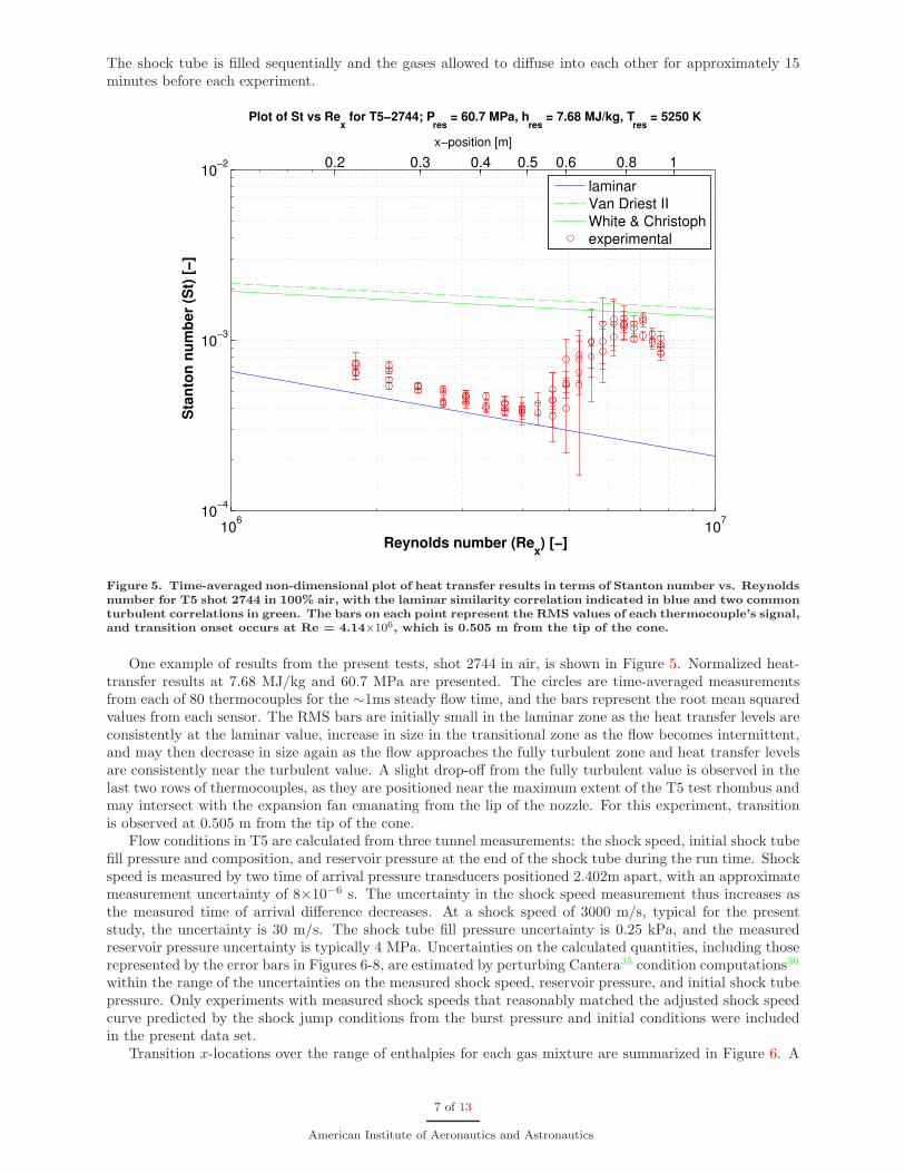
Figure 5. Time-averaged non-dimensional plot of heat transfer results in terms of Stanton number vs. Reynoldsnumber for T5 shot 2744 in 100% air, with the laminar similarity correlation indicated in blue and two commonturbulent correlations in green. The bars on each point represent the RMS values of each thermocouple’s signal,and transition onset occurs at Re = 4.14×106, which is 0.505 m from the tip of the cone.

One example of results from the present tests, shot 2744 in air, is shown in Figure 5. Normalized heat-transfer results at 7.68 MJ/kg and 60.7 MPa are presented. The circles are time-averaged measurementsfrom each of 80 thermocouples for the ∼1ms steady flow time, and the bars represent the root mean squaredvalues from each sensor. The RMS bars are initially small in the laminar zone as the heat transfer levels areconsistently at the laminar value, increase in size in the transitional zone as the flow becomes intermittent,and may then decrease in size again as the flow approaches the fully turbulent zone and heat transfer levelsare consistently near the turbulent value. A slight drop-off from the fully turbulent value is observed in thelast two rows of thermocouples, as they are positioned near the maximum extent of the T5 test rhombus andmay intersect with the expansion fan emanating from the lip of the nozzle. For this experiment, transitionis observed at 0.505 m from the tip of the cone.

Flow conditions in T5 are calculated from three tunnel measurements: the shock speed, initial shock tubefill pressure and composition, and reservoir pressure at the end of the shock tube during the run time. Shockspeed is measured by two time of arrival pressure transducers positioned 2.402m apart, with an approximatemeasurement uncertainty of 8×10−6 s. The uncertainty in the shock speed measurement thus increases asthe measured time of arrival difference decreases. At a shock speed of 3000 m/s, typical for the presentstudy, the uncertainty is 30 m/s. The shock tube fill pressure uncertainty is 0.25 kPa, and the measuredreservoir pressure uncertainty is typically 4 MPa. Uncertainties on the calculated quantities, including thoserepresented by the error bars in Figures 6-8, are estimated by perturbing Cantera35 condition computations36

within the range of the uncertainties on the measured shock speed, reservoir pressure, and initial shock tubepressure. Only experiments with measured shock speeds that reasonably matched the adjusted shock speedcurve predicted by the shock jump conditions from the burst pressure and initial conditions were includedin the present data set.

Transition x-locations over the range of enthalpies for each gas mixture are summarized in Figure 6. A

7 of 13

American Institute of Aeronautics and Astronautics

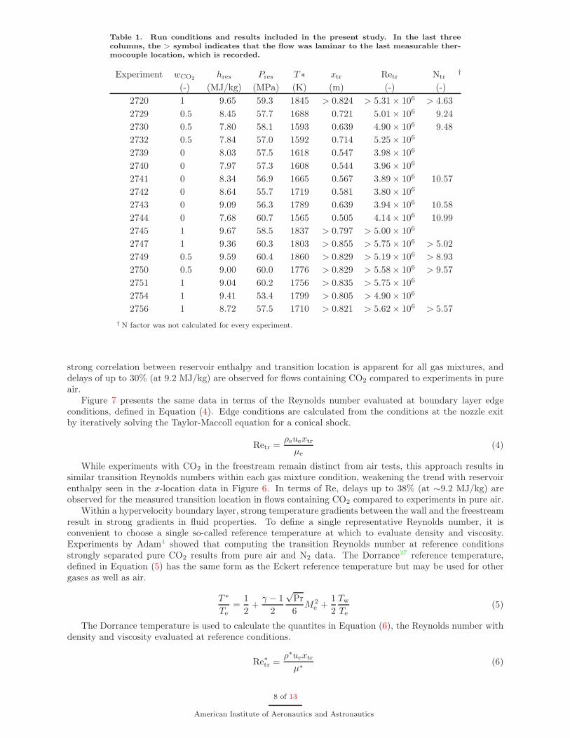
Table 1. Run conditions and results included in the present study. In the last threecolumns, the > symbol indicates that the flow was laminar to the last measurable ther-mocouple location, which is recorded.

Experiment wCO2 hres Pres T ∗ xtr Retr Ntr†

(-) (MJ/kg) (MPa) (K) (m) (-) (-)

2720 1 9.65 59.3 1845 > 0.824 > 5.31× 106 > 4.63

2729 0.5 8.45 57.7 1688 0.721 5.01× 106 9.24

2730 0.5 7.80 58.1 1593 0.639 4.90× 106 9.48

2732 0.5 7.84 57.0 1592 0.714 5.25× 106

2739 0 8.03 57.5 1618 0.547 3.98× 106

2740 0 7.97 57.3 1608 0.544 3.96× 106

2741 0 8.34 56.9 1665 0.567 3.89× 106 10.57

2742 0 8.64 55.7 1719 0.581 3.80× 106

2743 0 9.09 56.3 1789 0.639 3.94× 106 10.58

2744 0 7.68 60.7 1565 0.505 4.14× 106 10.99

2745 1 9.67 58.5 1837 > 0.797 > 5.00× 106

2747 1 9.36 60.3 1803 > 0.855 > 5.75× 106 > 5.02

2749 0.5 9.59 60.4 1860 > 0.829 > 5.19× 106 > 8.93

2750 0.5 9.00 60.0 1776 > 0.829 > 5.58× 106 > 9.57

2751 1 9.04 60.2 1756 > 0.835 > 5.75× 106

2754 1 9.41 53.4 1799 > 0.805 > 4.90× 106

2756 1 8.72 57.5 1710 > 0.821 > 5.62× 106 > 5.57

† N factor was not calculated for every experiment.

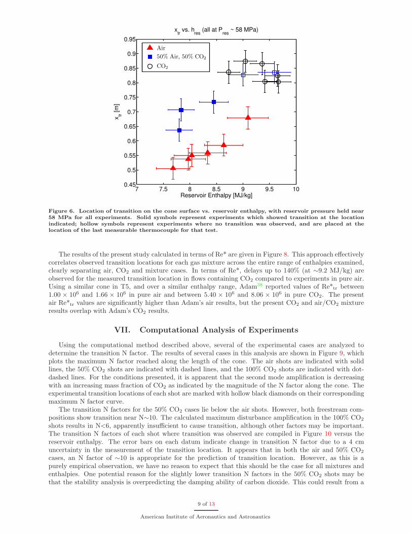
strong correlation between reservoir enthalpy and transition location is apparent for all gas mixtures, anddelays of up to 30% (at 9.2 MJ/kg) are observed for flows containing CO2 compared to experiments in pureair.

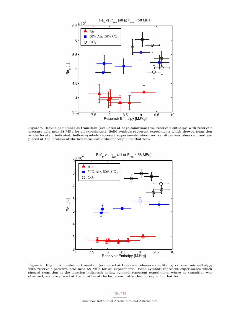
Figure 7 presents the same data in terms of the Reynolds number evaluated at boundary layer edgeconditions, defined in Equation (4). Edge conditions are calculated from the conditions at the nozzle exitby iteratively solving the Taylor-Maccoll equation for a conical shock.

Retr =ρeuextr

μe(4)

While experiments with CO2 in the freestream remain distinct from air tests, this approach results insimilar transition Reynolds numbers within each gas mixture condition, weakening the trend with reservoirenthalpy seen in the x-location data in Figure 6. In terms of Re, delays up to 38% (at ∼9.2 MJ/kg) areobserved for the measured transition location in flows containing CO2 compared to experiments in pure air.

Within a hypervelocity boundary layer, strong temperature gradients between the wall and the freestreamresult in strong gradients in fluid properties. To define a single representative Reynolds number, it isconvenient to choose a single so-called reference temperature at which to evaluate density and viscosity.Experiments by Adam4 showed that computing the transition Reynolds number at reference conditionsstrongly separated pure CO2 results from pure air and N2 data. The Dorrance37 reference temperature,defined in Equation (5) has the same form as the Eckert reference temperature but may be used for othergases as well as air.

T ∗

Te=

1

2+

γ − 1

2

√Pr

6M2

e +1

2

Tw

Te(5)

The Dorrance temperature is used to calculate the quantites in Equation (6), the Reynolds number withdensity and viscosity evaluated at reference conditions.

Re∗tr =ρ∗uextr

μ∗ (6)

8 of 13

American Institute of Aeronautics and Astronautics

7 7.5 8 8.5 9 9.5 100.45

0.5

0.55

0.6

0.65

0.7

0.75

0.8

0.85

0.9

0.95

xtr vs. h

res (all at P

res ~ 58 MPa)

Reservoir Enthalpy [MJ/kg]

x tr [m

]

Air

50% Air, 50% CO2

CO2

Figure 6. Location of transition on the cone surface vs. reservoir enthalpy, with reservoir pressure held near58 MPa for all experiments. Solid symbols represent experiments which showed transition at the locationindicated; hollow symbols represent experiments where no transition was observed, and are placed at thelocation of the last measurable thermocouple for that test.

The results of the present study calculated in terms of Re* are given in Figure 8. This approach effectivelycorrelates observed transition locations for each gas mixture across the entire range of enthalpies examined,clearly separating air, CO2 and mixture cases. In terms of Re*, delays up to 140% (at ∼9.2 MJ/kg) areobserved for the measured transition location in flows containing CO2 compared to experiments in pure air.Using a similar cone in T5, and over a similar enthalpy range, Adam38 reported values of Re*tr between1.00 × 106 and 1.66 × 106 in pure air and between 5.40 × 106 and 8.06 × 106 in pure CO2. The presentair Re*tr values are significantly higher than Adam’s air results, but the present CO2 and air/CO2 mixtureresults overlap with Adam’s CO2 results.

VII. Computational Analysis of Experiments

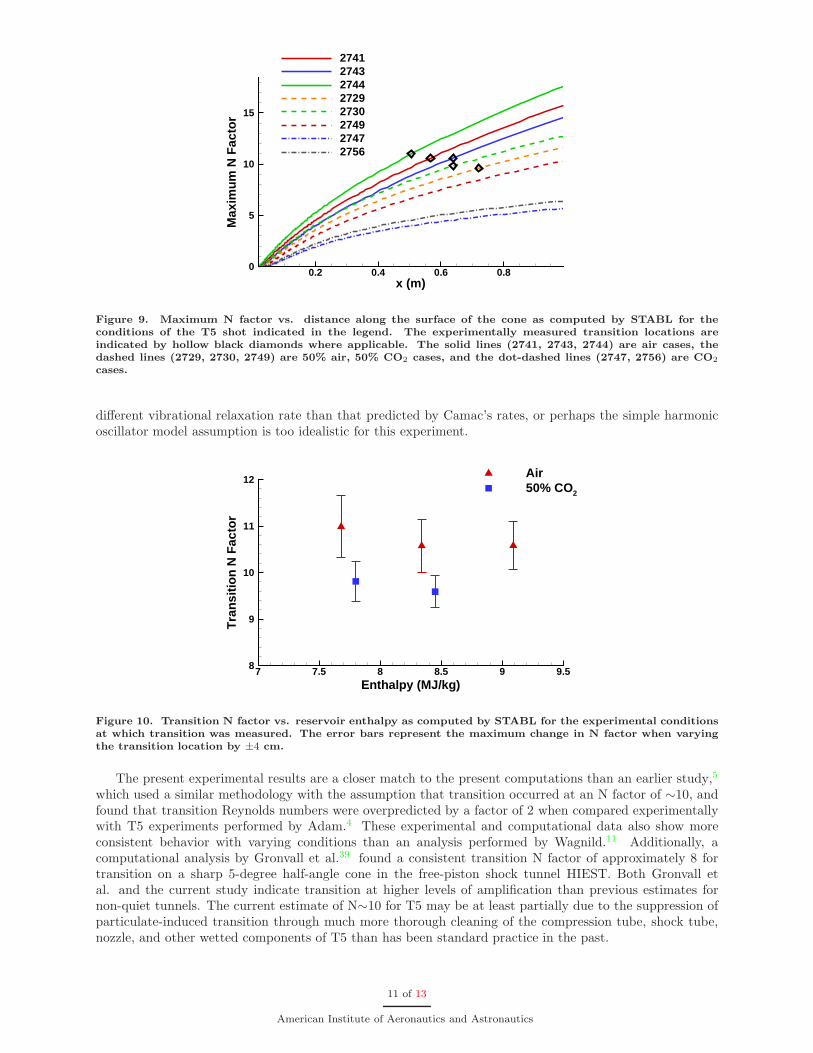
Using the computational method described above, several of the experimental cases are analyzed todetermine the transition N factor. The results of several cases in this analysis are shown in Figure 9, whichplots the maximum N factor reached along the length of the cone. The air shots are indicated with solidlines, the 50% CO2 shots are indicated with dashed lines, and the 100% CO2 shots are indicated with dot-dashed lines. For the conditions presented, it is apparent that the second mode amplification is decreasingwith an increasing mass fraction of CO2 as indicated by the magnitude of the N factor along the cone. Theexperimental transition locations of each shot are marked with hollow black diamonds on their correspondingmaximum N factor curve.

The transition N factors for the 50% CO2 cases lie below the air shots. However, both freestream com-positions show transition near N∼10. The calculated maximum disturbance amplification in the 100% CO2

shots results in N<6, apparently insufficient to cause transition, although other factors may be important.The transition N factors of each shot where transition was observed are compiled in Figure 10 versus thereservoir enthalpy. The error bars on each datum indicate change in transition N factor due to a 4 cmuncertainty in the measurement of the transition location. It appears that in both the air and 50% CO2

cases, an N factor of ∼10 is appropriate for the prediction of transition location. However, as this is apurely empirical observation, we have no reason to expect that this should be the case for all mixtures andenthalpies. One potential reason for the slightly lower transition N factors in the 50% CO2 shots may bethat the stability analysis is overpredicting the damping ability of carbon dioxide. This could result from a

9 of 13

American Institute of Aeronautics and Astronautics

7 7.5 8 8.5 9 9.5 103.5

4

4.5

5

5.5

6

6.5x 10

6 Retr vs. h

res (all at P

res ~ 58 MPa)

Reservoir Enthalpy [MJ/kg]

Re tr

[−]

Air

50% Air, 50% CO2

CO2

Figure 7. Reynolds number at transition (evaluated at edge conditions) vs. reservoir enthalpy, with reservoirpressure held near 58 MPa for all experiments. Solid symbols represent experiments which showed transitionat the location indicated; hollow symbols represent experiments where no transition was observed, and areplaced at the location of the last measurable thermocouple for that test.

7 7.5 8 8.5 9 9.5 102

3

4

5

6

7

8

9x 10

6 Re*tr vs. h

res (all at P

res ~ 58 MPa)

Reservoir Enthalpy [MJ/kg]

Re*

tr [−

]

Air

50% Air, 50% CO2

CO2

Figure 8. Reynolds number at transition (evaluated at Dorrance reference conditions) vs. reservoir enthalpy,with reservoir pressure held near 58 MPa for all experiments. Solid symbols represent experiments whichshowed transition at the location indicated; hollow symbols represent experiments where no transition wasobserved, and are placed at the location of the last measurable thermocouple for that test.

10 of 13

American Institute of Aeronautics and Astronautics

x (m)

Max

imu

m N

Fac

tor

0.2 0.4 0.6 0.80

5

10

15

27412743274427292730274927472756

Figure 9. Maximum N factor vs. distance along the surface of the cone as computed by STABL for theconditions of the T5 shot indicated in the legend. The experimentally measured transition locations areindicated by hollow black diamonds where applicable. The solid lines (2741, 2743, 2744) are air cases, thedashed lines (2729, 2730, 2749) are 50% air, 50% CO2 cases, and the dot-dashed lines (2747, 2756) are CO2

cases.

different vibrational relaxation rate than that predicted by Camac’s rates, or perhaps the simple harmonicoscillator model assumption is too idealistic for this experiment.

Enthalpy (MJ/kg)

Tra

nsi

tio

n N

Fac

tor

7 7.5 8 8.5 9 9.58

9

10

11

12 Air50% CO2

Figure 10. Transition N factor vs. reservoir enthalpy as computed by STABL for the experimental conditionsat which transition was measured. The error bars represent the maximum change in N factor when varyingthe transition location by ±4 cm.

The present experimental results are a closer match to the present computations than an earlier study,5

which used a similar methodology with the assumption that transition occurred at an N factor of ∼10, andfound that transition Reynolds numbers were overpredicted by a factor of 2 when compared experimentallywith T5 experiments performed by Adam.4 These experimental and computational data also show moreconsistent behavior with varying conditions than an analysis performed by Wagnild.11 Additionally, acomputational analysis by Gronvall et al.39 found a consistent transition N factor of approximately 8 fortransition on a sharp 5-degree half-angle cone in the free-piston shock tunnel HIEST. Both Gronvall etal. and the current study indicate transition at higher levels of amplification than previous estimates fornon-quiet tunnels. The current estimate of N∼10 for T5 may be at least partially due to the suppression ofparticulate-induced transition through much more thorough cleaning of the compression tube, shock tube,nozzle, and other wetted components of T5 than has been standard practice in the past.

11 of 13

American Institute of Aeronautics and Astronautics

VIII. Conclusions and Future Work

Consistent transition N factors greater than 10 have been found over a 5-degree half-angle in the T5hypervelocity shock tunnel for air flows with reservoir enthalpies above 7.68 MJ/kg and reservoir pressuresnear 58 MPa. N factors greater than 9 have been calculated for 50% air/CO2 mixtures at equivalent enthalpyand pressure conditions. Transition location is an increasing function of both the reservoir enthalpy and CO2

concentration. Addition of 50% CO2 by mass results in an increase in transition distance of Re* by a factorof two, but the N factor is comparable in all cases, N∼9–11. This suggests that the suppression of thesecond mode through the absorption of energy from acoustic disturbances through vibrational relaxation isa mechanism for delaying transition both in high-enthalpy carbon dioxide flows and, more usefully, high-enthalpy flows consisting of a mixture of CO2 and air.

These results are quite promising. Future work will include the installation of a premixing tank forstudies using fully mixed CO2 and air in the shock tube, to address concerns about completeness of thegaseous mixing process prior to each experiment; additional mass fraction cases; studies in gases other thanCO2; and ultimately continuation of the boundary-layer injection work begun in Jewell et al.12

Acknowledgments

The authors thank Mr. Nick Parziale for his assistance in running T5, Mr. Bahram Valiferdowsi forhis work with design, fabrication, and maintenance, and Prof. Hans Hornung for his advice and support.The experimental portion of this project was sponsored by the Air Force Office of Scientific Research underaward number FA9550-10-1-0491 and the NASA/AFOSR National Center for Hypersonic Research. Thecomputational work was sponsored by the Air Force Office of Scientific Research grant FA9550-10-1-0352.Sandia National Laboratories is a multi-program laboratory managed and operated by Sandia Corporation,a wholly owned subsidiary of Lockheed Martin Corporation, for the U.S. Department of Energy’s NationalNuclear Security Administration under contract DE-AC04-94AL85000. The views expressed herein are thoseof the authors and should not be interpreted as necessarily representing the official policies or endorsements,either expressed or implied, of AFOSR, Sandia, or the U.S. Government.

References

1Mack, L. M., “Boundary-layer linear stability theory. special course on stability and transition of laminar flow advisorygroup for aerospace research and development,” Tech. rep., 1984, AGARD Report No. 709.

2Malik, M. R., “Hypersonic flight transition data analysis using parabolized stability equations with chemistry effects,”Journal of Spacecraft and Rockets, Vol. 40, No. 3, 2003, pp. 332–344.

3Germain, P., The Boundary Layer on a Sharp Cone in High-Enthalphy Flow , Ph.D. thesis, California Institute ofTechnology, Pasadena, CA, 1993.

4Adam, P. H. and Hornung, H. G., “Enthalpy effects on hypervelocity boundary-layer transition: Ground test and flightdata,” Journal of Spacecrafts and Rockets, Vol. 34, No. 5, 1997.

5Johnson, H. B., Seipp, T. G., and Candler, G. V., “Numerical study of hypersonic reacting boundary layer transition oncones,” Physics of Fluids, Vol. 10, 1998, pp. 2676–2685.

6Fujii, K. and Hornung, H. G., “A Procedure to Estimate Absorption Rate of Sound Propagating Through High Temper-ature Gas,” Tech. rep., California Institute of Technology, Pasadena, CA, Aug. 2001, GALCIT Report FM2001.004.

7Fedorov, A. V., Malmuth, N. D., and Hornung, H. G., “Stabilization of hypersonic boundary layers by porous coatings,”AIAA journal , Vol. 39, No. 4, 2001, pp. 605–610.

8Rasheed, A., Hornung, H. G., Fedorov, A. V., and Malmuth, N. D., “Experiments on passive hypervelocity boundary-layercontrol using an ultrasonically absorptive surface,” AIAA Journal , Vol. 40, No. 3, 2002, pp. 481–489.

9Leyva, I. A., Laurence, S., Beierholm, A. W., Hornung, H. G., Wagnild, R., and Candler, G., “Transition delay inhypervelocity boundary layers by means of CO2/acoustic instability interactions,” 47th Aerospace Sciences Meeting , AIAA,Orlando, FL, 2009, AIAA 2009-1287.

10Wagnild, R. M., Candler, G. V., Leyva, I. A., Jewell, J. S., and Hornung, H. G., “Carbon Dioxide Injection for Hyper-velocity Boundary Layer Stability,” 48th Aerospace Sciences Meeting , AIAA, Orlando, FL, 2010, AIAA 2010-1244.

11Wagnild, R. M., High Enthalpy Effects on Two Boundary Layer Disturbances in Supersonic and Hypersonic Flow , Ph.D.thesis, University of Minnesota, Minneapolis, MN, 2012.

12Jewell, J. S., Leyva, I. A., Parziale, N. J., and Shepherd, J. E., “Effect of Gas Injection on Transition in HypervelocityBoundary Layers,” Proceedings of the 28th International Symposium on Shockwaves, Manchester, UK, 2011.

13Fedorov, A., “Transition and stability of high-speed boundary layers,” Annual Review of Fluid Mechanics, Vol. 43, 2011,pp. 79–95.

14Stetson, K. F., “Hypersonic boundary-layer transition,” Advances in Hypersonics, edited by J. Bertin, J. Periauz, andJ. Ballman, Birkhauser, Boston, MA, 1992, pp. 324–417.

15Kinsler, L. E., Frey, A. R., Coppens, A. B., and Sanders, J. V., Fundamentals of acoustics (Third Edition), John Wiley& Sons, Inc., New York, 1982.

12 of 13

American Institute of Aeronautics and Astronautics

16Clarke, J. F. and McChesney, M., The dynamics of real gases, Vol. 175, Butterworths, 1964.17Zeldovich, Y. B. and Raizer, Y. P., Physics of shock waves and high-temperature hydrodynamic phenomena, Academic

Press, New York, NY, 1967.18Camac, M., “CO2 relaxation processes in shock waves,” Fundamental Phenomena in Hypersonic Flow , edited by J. Hall,

Cornell University Press, 1966, pp. 195–215.19Hornung, H., “Performance data of the new free-piston shock tunnel at GALCIT,” 17th Aerospace Ground Testing

Conference, AIAA, Nashville, TN, 1992, AIAA 92-3943.20Hornung, H. and Belanger, J., “Role and techniques of ground testing for simulation of flows up to orbital speed,” 16th

Aerodynamic Ground Testing Conference, AIAA, Seattle, WA, 1990, AIAA 90-1377.21Marineau, E. C. and Hornung, H. G., “Modeling and calibration of fast-response coaxial heat flux gages,” 47th Aerospace

Sciences Meeting , AIAA, Orlando, FL, 2009, AIAA 2009-0737.22Candler, G. ., “Hypersonic nozzle analysis using an excluded volume equation of state,” AIAA 2005-5202.23Spalart, P. R. and Allmaras, S. R., “A one-equation turbulence model for aerodynamic flows,” 30th Aerospace Sciences

Meeting and Exhibit , AIAA, Reno, NV, 1992, AIAA 92-0439.24Catris, S. and Aupoix, B., “Density corrections for turbulence models,” Aerospace Science and Technology , Vol. 4, No. 1,

2000, pp. 1–11.25Johnson, H. B., Thermochemical Interactions in Hypersonic Boundary Layer Stability , Ph.D. thesis, University of Min-

nesota, Minneapolis, MN, 2000.26Johnson, H. B. and Candler, G. V., “Hypersonic boundary layer stability analysis using PSE-Chem,” 35th Fluid Dynamics

Conference and Exhibit , AIAA, 2005, AIAA 2005-5023.27Schneider, S. P., “Effects of high-speed tunnel noise on laminar-turbulent transition,” Journal of Spacecraft and Rockets,

Vol. 38, No. 3, 2001, pp. 323–333.28Park, C., Howe, J. T., Jaffe, R. L., and Candler, G. V., “Review of Chemical-Kinetic Problems of Future NASA Missions,

II: Mars Entries,” Journal of Thermophysics and Heat transfer , Vol. 8, No. 1, 1994, pp. 9–23.29Bose, D. and Candler, G. V., “Thermal Rate Constants of the N2 + O → NO+ N Reaction Using Ab Initio 3A′′ and

3A′ Potential Energy Surfaces,” Journal of Chemical Physics, Vol. 104, No. 8, 1996, pp. 2825–2833.30Bose, D. and Candler, G. V., “Thermal Rate Constants of the O + N → NO + O Reaction Based on the 2A′ and 4A′

Potential-Energy Surfaces,” Journal of Chemical Physics, Vol. 107, No. 16, 1997, pp. 6136–6145.31Park, C., Nonequilibrium Hypersonic Aerothermodynamics, Wiley, New York, 1990.32McBride, B. J., Zehe, M. J., and Gordon, S., “NASA Glenn coefficients for calculating thermodynamic properties of

individual species,” Tech. rep., 2002, Report TP-2002-21155.33Vincenti, W. G. and Kruger, C. H., Introduction to Physical Gas Dynamics, Wiley, New York, 1965.34Wagnild, R. M., Candler, G. V., Subbareddy, P., and Johnson, H., “Vibrational Relaxation Effects on Acoustic Distur-

bances in a Hypersonic Boundary Layer over a Cone,” 50th Aerospace Sciences Meeting , AIAA, Nashville, TN, 2012, AIAA2012-0922.

35Goodwin, D., “Cantera: An object-oriented software toolkit for chemical kinetics, thermodynamics, and transport pro-cesses,” Available: http://code.google.com/p/cantera, 2009, Accessed: 12/12/2012.

36Browne, S., Ziegler, J., and Shepherd, J., “Numerical solution methods for shock and detonation jump conditions,” Tech.rep., California Institute of Technology, Pasadena, CA, July 2008, GALCIT Report FM2006.006.

37Dorrance, W. H., Viscous hypersonic flow: theory of reacting and hypersonic boundary layers, McGraw-Hill, 1962.38Adam, P. H., Enthalpy Effects on Hypervelocity Boundary Layers, Ph.D. thesis, California Institute of Technology,

Pasadena, CA, 1997.39Gronvall, J. E., Johnson, H. B., and Candler, G. V., “Boundary Layer Stability Analysis of the Free-Piston Shock Tunnel

HIEST Transition Experiments,” 48th Aerospace Sciences Meeting , AIAA, Orlando, FL, 2010, AIAA 2010-0896.

13 of 13

American Institute of Aeronautics and Astronautics