traffic generated by mixed-use developments six-region ... · e-mail: [email protected]...

Traffic Generated by Mixed-UseDevelopments—Six-Region Study UsingConsistent Built Environmental Measures

Reid Ewing1; Michael Greenwald2; Ming Zhang3; Jerry Walters4; Mark Feldman5;Robert Cervero6; Lawrence Frank7; and John Thomas8

Abstract: Current methods of traffic impact analysis, which rely on rates and adjustments from the Institute of Transportation Engineers,are believed to understate the traffic benefits of mixed-use developments (MXDs), leading to higher exactions and development fees thannecessary and discouraging otherwise desirable developments. The purpose of this study is to create new methodology for more accuratelypredicting the traffic impacts of MXDs. Standard protocols were used to identify and generate data sets for MXDs in six large and diversemetropolitan regions. Data from household travel surveys and geographic information system (GIS) databases were pooled for these MXDs,and travel and built environmental variables were consistently defined across regions. Hierarchical modeling was used to estimate models forinternal capture of trips within MXDs, walking and transit use on external trips, and trip length for external automobile trips. MXDs withdiverse activities on-site are shown to capture a large share of trips internally, reducing their traffic impacts relative to conventional suburbandevelopments. Smaller MXDs in walkable areas with good transit access generate significant shares of walk and transit trips, thus alsomitigating traffic impacts. Centrally located MXDs, small and large, generate shorter vehicle trips, which reduces their impacts relativeto outlying developments. DOI: 10.1061/(ASCE)UP.1943-5444.0000068. © 2011 American Society of Civil Engineers.

CE Database subject headings: Traffic management; Assessment; Environmental issues.

Author keywords: Mixed-use development; Trip generation; Internal capture; Traffic impact assessment.

Introduction

Mixed-use development (MXD) is a signature feature of smartgrowth, New Urbanism, and other contemporary land-usemovements aimed at reducing the private automobile’s dominance

in suburban America. By putting offices, shops, restaurants,residences, and other codependent activities in close proximityto each other, MXD shortens trips and thus allows what mightotherwise be external car trips to become internal walk, bike, ortransit trips. This in turn can reduce the vehicle miles generatedby an MXD relative to what it would be if the same activities wereseparated in single-use developments. Fewer vehicle miles traveled(VMT) not only relieves traffic congestion but also reduces green-house gas (GHG) emissions, air pollution, and fuel consumption.MXDs are also promoted for their supply side benefits, such aspossibilities for shared parking and economizing on roadwayand related infrastructure expenditures (because peak travel periodsoften differ between offices, retail, and other uses, enabling invest-ments to be descaled) (Cervero 1988).

A diverse group of stakeholders has a vested interest in thetraffic impacts of MXDs. The replacement of off-site car trips withon-site walking or cycling or (for larger mixed-use sites) on-sitetransit or driving matters to developers who want smooth-flowingtraffic conditions to help market their projects, to communities thatwant to keep existing residents safe from traffic impacts, and totraffic engineers whose very profession is devoted to facilitatingtraffic flows but often harbor some skepticism about the trafficbenefits of MXDs.

Accurately estimating the proportion of trips captured internallyby MXDs is vitally important if communities are to accuratelyassess their traffic impacts and reward such projects through lowerexactions and development fees or expedited project approvals.However, lacking a reliable methodology for adjusting trip gener-ation estimates, communities face a dilemma when assessing MXDproposals: do they err on the conservative side by downplayinginternal capture and thereby potentially discourage worthwhileprojects, or err on the liberal side and risk unmitigated traffic

1Professor, Dept. of City and Metropolitan Planning, Univ. of Utah, 375S. 1530, E. Salt Lake City, UT 84103 (corresponding author). E-mail:[email protected]

2Senior Transportation Planner, Lane Council of Governments, 859Willamette St., Suite 500, Eugene, OR 97401; formerly, Lead Modelerand Analyst/GIS Specialist, Urban Design 4 Health, Inc., P.O. Box85508, Seattle, WA 98145. E-mail: [email protected]

3Associate Professor, Community and Regional Planning, Univ. ofTexas at Austin, 1 University Station, B7500, Austin, TX 78712. E-mail:[email protected]

4Principal and Chief Technical Officer, Fehr & Peers, 100 Pringle Ave.,Suite 600, Walnut Creek, CA 94596. E-mail: [email protected]

5Transportation Engineer, Fehr & Peers, 100 Pringle Ave., Suite 600,Walnut Creek, CA 94596. E-mail: [email protected]

6Professor, Dept. of City and Regional Planning, Univ. of California,Berkeley, 228 Wurster Hall, Berkeley, CA 94720-1850. E-mail: [email protected]

7Associate Professor, School of Environmental Health, Univ. of BritishColumbia, 3rd Floor—2206 East Mall. Vancouver, BC V6T 1Z3 Canada.E-mail: [email protected]

8Policy Analyst, Office of Sustainable Communities, US EPA, 1200Pennsylvania Ave. NW Mailcode 1807T, Washington, DC 20816. E-mail:[email protected]

Note. This manuscript was submitted on December 11, 2009; approvedon October 11, 2010; published online on October 19, 2010. Discussionperiod open until February 1, 2012; separate discussions must be submittedfor individual papers. This paper is part of the Journal of Urban Planningand Development, Vol. 137, No. 3, September 1, 2011. ©ASCE, ISSN0733-9488/2011/3-248–261/$25.00.

248 / JOURNAL OF URBAN PLANNING AND DEVELOPMENT © ASCE / SEPTEMBER 2011

Downloaded 14 Sep 2011 to 192.245.136.3. Redistribution subject to ASCE license or copyright. Visithttp://www.ascelibrary.org

http://dx.doi.org/10.1061/(ASCE)UP.1943-5444.0000068




impacts? Often, the “do no harm” sentiment prevails: when in doubt,go with conventional practices, which, with MXD proposals, typi-cally means only a small downward adjustment in estimated trips, ifany adjustment at all.

In addition to getting internal capture estimates right, accurateassessments of MXD projects also depend on estimating the shareof external trips served by alternative modes (e.g., transit and walk-ing). These must also be subtracted from nominal trip generationrates to estimate the net impacts of MXDs on traffic and VMT.

Community acceptance depends on whether a proposedMXD isperceived as a good neighbor. Exaggerated estimates of a project’straffic generation can heighten concerns about congestion, commu-nity image and character, and even public health and safety. Animby backlash can add substantially to the time and expenseof securing project approval, and can result in the project beingscaled back to a level at which elected officials feel that the tripgeneration is more acceptable. However, the market demand forthe development that is disallowed does not vanish and more oftenthan not ends up in another location, often at a lower density and ina less mixed-use configuration. The end result can be more trafficand higher overall VMT than if the original MXD proposal hadbeen approved.

Traffic generation estimates have supply-side impacts, affectingproject design and cost. This includes the most obvious compo-nents, such as street widths, parking supply, and access pointdesign, and secondary effects on the design and cost of ancillaryinfrastructure like storm water drainage systems. Within con-strained sites, overdesign of traffic elements can limit the spaceavailable for revenue-producing land uses and increase other de-velopment costs; forcing, for example, the rerouting of utilities toaccommodate traffic-handling infrastructure.

Statutory laws also place pressure on getting the traffic estimatesfor MXDs right. The formal National Environmental Policy Act(NEPA) process and state-level environmental reviews rely on traf-fic generation estimates to assess impacts and dictate a project’smitigation measures. Estimates that exaggerate negative impactsincrease the likelihood a project will be judged as a significantthreat to environmental quality. This leads to more rigorous analy-sis and reporting of a wide array of potential secondary impacts,such as the growth inducing effects of the additional required trafficcapacity. It also prompts a more protracted discussion of commu-nity concerns through formal public involvement, document re-view, comment/response periods, and certification protocols. Inaddition, it can incorrectly trigger a review of other impacts suchas noise, air quality, energy use, and greenhouse gas emissions.

Development fee programs rely heavily on traffic generationestimates. As the most comprehensive and widely used referenceon the subject, the Trip Generation report of the Institute of Trans-portation Engineers (ITE) (2008) has become the principal datasource for setting transportation development fee rates. Most cities,counties, and regional agencies opt for uniformity rather thanaccuracy in this regard. In the interest of standardization of assump-tions and approach, many jurisdictions rely on the numbers inTrip Generation to quantify traffic impacts and mitigation feeschedules. The unquestioning use of the ITE report can unreason-ably jeopardize a MXD project’s approval, financial feasibility, anddesign quality.

Conventional Traffic Impact Analysis

Virtually all traffic impact analyses rely on the ITE Trip Generationreport (2008). The ITE rates are largely representative of individual,single-use suburban developments whose trips are by private

vehicle and whose origins or destinations lie outside the develop-ment. Quoting the report: “Data were primarily collected at subur-ban localities with little or no transit service, nearby pedestrianamenities, or travel demand management (TDM) programs.” Rec-ognizing but not resolving this limitation, Trip Generation advises:“At specific sites, the user may want to modify the trip generationrates presented in this document to reflect the presence of publictransportation service, ridesharing or other TDM measures, en-hanced pedestrian and bicycle trip-making opportunities, or otherspecial characteristics of the site or surrounding area.” Unfortu-nately, the desire among traffic engineers for standardization andsubstantial documented evidence prevents them from taking thisadvice in the vast majority of cases.

Even setting aside the variety and complexity of mixed-use de-velopments, the reliability of Trip Generation for evaluating simplesingle-use developments is less than one might assume. For exam-ple, for the most widely studied land-use category within the report,single-family residential, the average ITE Trip Generation dailyrate is 9.6 vehicle trips per dwelling unit, but the standard deviationis 3.7, almost 40% of the mean. Even for this most uniform of land-use types, when described in terms of a single descriptive variable(number of dwelling units), the 9.6 ITE trip generation figure usedin impact study guidelines and fee ordinances throughout theUnited States is just a midpoint in a standard deviation range of5.9 to 13.3 vehicle trips per dwelling. The standard deviationsfor other common and well-studied land-use types (e.g., officebuildings and shopping centers) are at least �50% of the meanvalues. Clearly, trip generation estimation is far from a precisescience.

Professor Donald Shoup of UCLA has been particularly criticalof Trip Generation for the following reasons: the false precisionwith which average trip generation rates are presented, the smallsamples upon which average rates and regression equations arebased, the insignificance of regression coefficients and constants,the implicit assumption that trip generation increases with buildingsize, and the disregard of factors other than building size in theregression analyses. Pointing to the need to represent land-use in-teractions more carefully, Shoup remarks, “Floor area is only oneamong many factors that influence vehicle trips at a site, and weshould not expect floor area or any other single variable to accu-rately predict the number of vehicle trips at any site or land-use”(Shoup 2003).

As an indication of just how far off the mark ITE rates may land,the Transit Cooperative Research Program (TCRP) recently fundeda study of the trip generating characteristics of transit-oriented de-velopments (TODs) (Cervero and Arrington 2008). The aim was toseed the ITE Trip Generation report with original and reliable tripgeneration data for one important TOD land-use—housing—withthe expectation that other TOD land uses will be added later. For allTOD housing projects studied, weekday vehicle trip rates wereconsiderably below the ITE average rate for similar uses. Takingthe weighted average across the 17 case-study projects, TOD hous-ing projects, which included both multifamily and single-familyresidential units, generated approximately 44% fewer vehicle tripsthan predicted by the ITE report (3.8 trips per dwelling unit forTOD housing versus 6.7 trips per dwelling unit by ITE estimatesfor the site-specific mixes of multi- and single-family residences).

ITE Method for MXDs

For mixed-use development projects, Chapter 7 of Trip GenerationHandbook (2004) outlines a procedure for estimating the propor-tion of trips that remain within the development (i.e., the internal

JOURNAL OF URBAN PLANNING AND DEVELOPMENT © ASCE / SEPTEMBER 2011 / 249


capture rate), and hence place no strain on the external streetnetwork. An ITE member survey found that nearly two-thirds ofpractitioners estimate internal capture rates using this procedure.The procedure works as follows:1. The analyst determines the amounts of different land-use

types (residential, retail, and office) contained within thedevelopment.

2. These amounts are multiplied by ITE’s per-unit trip generationrates to obtain a preliminary estimate of the number of vehicletrips generated by the site. This preliminary estimate is whatthe site would be expected to generate if there were no inter-actions among the on-site uses.

3. The generated trips are then reduced by a certain percentage toaccount for internal-capture of trips within MXDs. The reduc-tions are based on lookup tables. The share of internal tripsfrom the appropriate lookup table is multiplied by totalnumbers of trips generated by a given use to obtain an initialestimate of internal trips for each producing use and attractinguse.

4. For each pair of land uses, productions and attractions arereconciled such that the number of internal trips produced byone use just equals the number attracted by the other use. Thelesser of the two estimates of internal trips constrains the num-ber of internal trips generated by the other use.

Strengths of the Current ITE Method

From the viewpoint of the practicing engineer, the ITE internalcapture methodology has some important advantages:1. It seems objective. Two analysts given the same data will arrive

at exactly the same result. There is no room for negotiation orinterpretation (and therefore no reason to pressure the analystinto skewing the results in a predetermined direction).

2. It seems logical. Most engineers readily accept the idea that thedegree of internalization will be determined by how well theproductions and attractions match for each trip purpose.

3. It is fast. With a spreadsheet template, an analyst can input thedata and have an answer in a matter of minutes.Viewed another way, any new methodology that lacks these

qualities may not find wide acceptance within the engineeringcommunity.

Weaknesses of the Current Method

The ITE methodology also has major shortcomings:1. The two lookup tables are based on data for a “limited number

of multiuse sites in Florida” (specifically, three sites analyzedby the Florida Department of Transportation, ITE 2004). Theaccuracy of forecasts is thus dependent on how closely the sitebeing analyzed matches the sites used in the tables’ creation.The fact that the data are drawn from the suburbs of Floridacasts doubt on the applicability to other parts of the country.The handbook acknowledges this problem and instructs theanalyst to find analogous sites locally and collect his own datato produce locally valid lookup tables.

2. The land-use types and adjustments embodied in the lookuptables are limited to the three uses: residential, retail, andoffices. The traffic impacts of other mixed uses cannot beassessed.

3. The scale of development is disregarded. Clearly, a large sitewith many productions and attractions is more likely to pro-duce matches than a small site, and the lookup tables forlarge sites should have higher cell percentages than the tablesfor small sites. Development scale was the most significantinfluence on internal capture rates in a study of South FloridaMXDs, and more than half of all trips were found to be

internalized by community-scale MXDs, far in excess ofany rate obtainable with the handbook method (Ewing et al.2001).

4. The land-use context of development projects is ignored. Com-mon sense and the literature tell us that projects in remotelocations are more likely to capture trips on-site than thosesurrounded by competing trip attractions. For MXDs in SouthFlorida, the second most important determinant of internal cap-ture rates was accessibility to the rest of the region (secondafter the scale of development). Conversely, projects in areasof high accessibility are more likely to generate walk trips toexternal destinations.

5. The possibility of mode shifts for well-integrated, transit-served sites is not explicitly considered. This may not biasresults for free-standing sites, but infill projects within anurban context may capture few trips internally but still havesignificant vehicle trip reductions relative to the ITE rates.

6. The length of external private vehicle trips is not considered.The ITE methodology deals with trip generation, not trafficgeneration. Clearly, in terms of roadway congestion, emis-sions, and other impacts, a 10-mile trip has a greater impactthan a 5-mile trip. Trip distribution is an ad hoc process underthe ITE methodology.

Parallel Efforts

There would seem to be two ways to refine ITE trip generationestimates of MXDs. One, a bottom-up approach, would add tothe paltry set of development projects that currently constitutethe ITE database on MXDs, analyze in detail this larger sample’strip-making characteristics, and then derive a set of more completeadjustments to ITE trip rates. In an effort parallel to our own, theNational Cooperative Highway Research Program (NCHRP) istaking this approach in NCHRP Project 8-51, “Enhancing InternalTrip Capture Estimation for Mixed-Use Developments.” Addingfour sites to the three that currently form the basis for internalcapture calculations in ITE’s Trip Generation Handbook (2004),the project has developed an estimation procedure that includesa proximity adjustment to account for project size and layout.

A second approach, more top down in nature, would assembleenough data on MXDs to estimate statistical models of trafficgeneration in terms of standard built environmental variables,the so-called “D” variables of density, diversity, design, destinationaccessibility, distance to transit, and development scale. Taking thisapproach, Ewing et al. (2001) modeled internal capture rates for 20mixed-use communities in South Florida. For the 20 communities,internal capture rates ranged from 0 to 57% of all trip ends gen-erated by the community.

To explain this variation, internal capture rates were modeled interms of land-use and accessibility measures. The variable thatproved most strongly related to internal capture was neither land-use mix nor density, but the size of the community itself. The twocommunities with the highest internal capture rates, Wellington andWeston, also are the largest, each having more than 30,000 resi-dents and 5,000 jobs. Indeed, these two communities are largeenough to have incorporated as their own small cities. The secondmost important variable was regional accessibility, which wasinversely related to internal capture rates. Both of these commun-ities are on the western edge of development in Southeast Florida,far from other population centers.

Owing to size and inaccessibility, these communities capture amuch higher percentage of trips internally than, for example, thehigher density and better-mixed Miami Lakes. However, Miami



Lakes doubtless generates shorter auto trips and many more walk,bicycle, and transit trips than the other two. Its overall impact on theregional road network is almost certainly less.

The validity and reliability of Ewing et al.’s results are limited bythe small sample, limited geography coverage, and small number ofbuilt environmental variables. The present study improves on theearlier study by, in this order: (1) pooling travel and built environ-mental data for 239 MXDs in six diverse regions; (2) consistentlydefining travel outcomes and built environmental variables forthese MXDs and regions; (3) estimating models of internal capture,external walk and transit choice, and external private vehicle triplength using hierarchical modeling methods; and (4) validatingthe results through comparison to traffic counts at an independentset of mixed-use sites in various parts of the United States.

Conceptual Framework

In travel research, urban development patterns have come to becharacterized by “D” variables. The original “three Ds,” coinedby Cervero and Kockelman (1997), are density, diversity, anddesign. Additional Ds have been labeled since then: destinationaccessibility, distance to transit, and demographics (Ewing andCervero 2001, 2010). An additional D variable is relevant to thisanalysis: development scale.

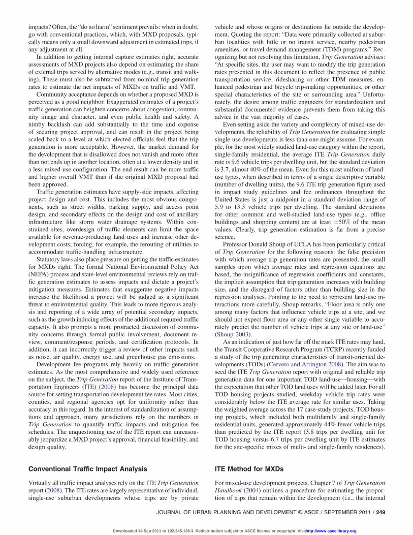
The theory of rational consumer choice underlies this study. It iswell articulated elsewhere (for example, Crane 1996; Boarnet andCrane 2001; Cervero 2002; Zhang 2004; Cao et al. 2009). Travelto/from MXDs is conceived as a series of choices that depend onthe D variables (see conceptual framework in Fig. 1). The choicesrelate directly to the methodology this paper is proposing to adjustITE trip generation rates downward.

The first adjustment to ITE rates is for trips that remain withinthe development. Destination choice is conceived as dichotomous.A traveler may choose a destination within the development, or adestination outside the development. Internal trips are treated as100% deductions from ITE trip generation rates.

Then, for trips that leave the development, adjustments aremade for walking and transit use. Mode choices are conceivedas dichotomous. For external trips, a traveler may choose to walkor not. Likewise, the traveler may choose to use transit or not.Walking and transit use may be treated as 100% deductions from

ITE trip generation rates, or may be treated as partial offsets. It isreasonable to assume that transit trips substitute for automobiletrips, but walk trips may supplement or substitute for automobiletrips. The study team plans to propose substitution rates based on areview of literature.

Finally, for external personal vehicle trips, the traveler choosesa destination. This destination may be near or far. This outcomevariable is continuous rather than dichotomous.

The D variables in Fig. 1 are characteristics of travelers, MXDs,and regions, as defined in the following. The D variables determine,moderate, mediate, and confound travel decisions.

Sample Selection

A main criterion for inclusion of regions in this study was dataavailability. Regions had to offer:1. Regional household travel surveys with XY coordinates for

trip ends, so we could distinguish trips to, from, and withinsmall MXDs; and

2. Land use databases at the parcel level with detailed land-useclassifications, so we could study land-use intensity and mixdown to the parcel level.Most U.S. regions fall short on one or both counts. Although

nearly all metropolitan planning organizations (MPOs) haveconducted regional household travel surveys as the basis for thecalibration of regional travel demand models, most have geocodedtrip ends only at the relatively coarse geography of traffic analysiszones. Likewise, although most MPOs have historical land-usedatabases that are used in model calibration, these too provide dataonly for the relatively coarse geography of traffic analysis zones.Traffic analysis zones vary in size from region to region, but as ageneral rule, are equivalent to census block groups. They are largerelative to many MXDs, and in any event, will ordinarily notcoincide with MXD boundaries.

Thirteen regional household travel databases were identifiedthat met the first criterion. This was narrowed down to six regionsbased on the availability of parcel-level land-use data and theexperience of planning researchers who had worked with these datasets.

All six travel databases were derived from large-scale householdtravel diary surveys. All allowed the writers to classify trips bypurpose and mode of travel. All allowed us to control for socioeco-nomic characteristics of travelers that may confound interactionsbetween the built environment and travel. All had already beenlinked to built environmental databases. Although the specificvariables differed somewhat from database to database, it was pos-sible to reconcile differences and specify equivalent models. Also,although the years of the surveys differed, it was possible to controlfor these and other fixed effects at the regional level in a three-levelhierarchical model.

Identifying MXDs

The ITE definition of multiuse development was modified to createa generic definition of MXD that would encompass many existingareas with interconnected, mixed land-use patterns:

“A mixed-use development or district consists of two or moreland uses between which trips can be made using local streets,without having to use major streets. The uses may includeresidential, retail, office, and/or entertainment. There maybe walk trips between the uses.”

To identify MXDs in the six study regions at the dates of themost recent regional household travel surveys, the team used aFig. 1. Traffic impact adjustments



bottom-up, expert-based process in which planners for the differentlocalities were queried about MXDs within their boundaries. Usingthis approach, a definition of an MXD was read to local plannersover the phone, and they were asked to name, identify the boun-daries, and list the uses contained within such areas. In two of thesix regions, local traffic engineers and ITE members were asked toreview the selected sites to confirm that they met the criteria nor-mally applied by practitioners to identify mixed-use developments.

Final Samples

A total of 239 MXDs were identified, ranging from a low of 24 inAtlanta to a high of 59 in Boston. Site characteristics ranged fromcompact infill sites near the region’s core to low-rise freeway ori-ented developments. The 239 survey sites varied in population andemployment densities, mix of jobs and housing, presence or ab-sence of transit, and location within the region. The sites rangedin size from less than five acres to over 2,000 acres, and over15,000 residents and employees.

Sample statistics are shown in Table 1. The regions that contrib-ute modest numbers of trip ends to the sample still add statisticalpower. The importance of Boston, Houston, and Sacramento lies inthe number of MXDs each contributes, not in the number of tripends. Also, the inclusion of the three regions doubles the number ofregions in the sample. In a hierarchical analysis, statistical power islimited by the number of degrees of freedom at each level of analy-sis. There are ample cases at Level 1, the trip end level, but a short-age of cases at Level 2, the MXD level, and a severe shortage atLevel 3, the regional level.

RiverPlace, a classic MXD just south of downtown Portland, isone of the 239 MXDs in our sample (Fig. 2). Its internal capturerate is a surprisingly high 36%. Of the external trips, 14% are made

by walking and 9% by transit. Its external auto trips average7.7 miles. According to the National Household Travel Surveyof 2009, 14% of Portland’s trips are by walking, and 2% are bytransit. The average vehicle trip length in the Portland ConsolidatedMetropolitan Statistical Area is 8.9 miles. On balance, the trafficimpact of RiverPlace is a fraction of the regional average.

Variables

In this study, all seven types of D variables were measured and usedto predict the travel characteristics of MXDs (Tables 2 and 3). Therichness of the data sets varies from region to region. Portland andAtlanta have the most complete data sets. Houston and Sacramentohave the least complete data sets. Sidewalk data, for example, areonly available for Atlanta and Portland. Floor area ratios are onlyavailable for Atlanta, Portland, and Seattle. Measures of job mix areonly available for Atlanta, Boston, Portland, and Seattle.

To maximize the sample of MXDs, the writers decided to limitour analysis to built environmental variables available for all sixregions. This also simplifies the use of the resulting models bypractitioners, who may have incomplete data on their projects ortheir surroundings.

There is great variation in internal capture rates from MXD toMXD and region to region. Across regions, average internal cap-ture rates vary from a low of 15.9% in Portland to a high of 31.1%for Houston (Table 4). The high rate for Houston may reflect thefact that Houston’s MXDs are, in general, larger and more remotelylocated than those in other regions. Many are standalone master-planned communities.

In all household travel surveys, automobile, walk, and transit(bus or rail, where available) are identified as separate modes oftravel. Bicycle is as well, but samples are too small to be reliablyanalyzed. In all regions, the dominant mode for external trips to/from MXDs is the automobile (“private motor vehicle”). Theessential choices facing travelers are to walk or use an automobile,or to take transit or use an automobile. For external trips, averagemode shares by walking and transit combined vary from a low of3.3% for Sacramento to a high of 28.4% for Boston (Table 4).

Of the 35,877 trip ends generated by these MXDs, 6,378(17.8%) involved trips within the mixed-use site, another 2,099(5.9%) involved trips entering or leaving the site via walking,and another 1,995 (5.6%) involved trips entering or leaving viatransit. Thus, on average, a total of 29% of the trip ends generatedby mixed-use developments put no strain on the external street net-work and should be deducted from ITE trip rates for standalonesuburban developments.

Trip distances are also variable across regions. For external autotrips, average distances range from 4.6 miles for MXDs in Bostonto 13.9 miles for MXDs in Houston (Table 4). Again, this reflectsthe size and remoteness of Houston’s MXDs.

Table 5 provides comparable data for trips internal to MXDs. Infour of the six regions, approximately half of the internal trips arewalk trips, and auto trips are short. For these regions, it may bereasonable to ignore the contribution of internal trips to regionalVMT and emissions, particularly since internal trips are onlyapproximately 16% of all trips produced by or attracted to theseMXDs. For the remaining two regions, with their large master-planned communities, the share of walk trips is low, and auto tripsare relatively long. For these regions, the contribution of internaltrips to regional VMT and emissions is significant. Although thesetrips may not contribute to area-wide congestion, they should beconsidered in VMT and emissions calculations.

Table 1. Sample Statistics

Surveyyear MXDs

Mean acreageper MXD

Totaltrip ends

Mean tripends per MXD

Atlanta 2001 24 287 6,167 257

Boston 1991 59 175 3,578 61

Houston 1995 34 401 1,584 47

Portland 1994 53 116 6,146 116

Sacramento 2000 25 179 2,487 99

Seattle 1999 44 207 15,915 362

Total 239 211 35,877 150

Fig. 2. (Color) RiverPlace at eye level



Table 2. Variable Definition and Description

Outcome variables Definition

INTERNAL Dummy variable indicating that a trip remains internal to the MXD (1 ¼ internal, 0 ¼ external).

WALK Dummy variable indicating that the travel mode on an external trip is walking (1 ¼ walk, 0 ¼ other).

TRANSIT Dummy variable indicating that the travel mode on an external trip is public bus or rail (1 ¼ transit, 0 ¼ other).

TDIST Network trip distance between origin and destination locations for an external private vehicle trip, in miles.

Explanatory variables

Level 1 traveler/household level

CHILD Variable indicating that the traveler is under 16 years of age (1 ¼ child, 0 ¼ adult).

HHSIZE Number of members of the household.

VEHCAP Number of motorized vehicles per person in the household.

BUSSTOP Dummy variable indicating that the household lives within 1=4 mile of a bus stop (1 ¼ yes, 0 ¼ no)

Level 2 MXD explanatory variables

AREA Gross land area of the MXD in square miles.

POP Resident population within the MXD; prorated sum of the population for the census block groups that intersect the MXD. Prorating

was done by calculating density of population per residential acre (tax lots designated single-family or multifamily) for the entire

census block group, then multiplying the density by the amount of residential acreage within the block group contributing to the

MXD, and finally, summing over all block groups intersecting the MXD area. For Houston, data at the traffic analysis zone (TAZ)

level were prorated.

EMP Employment within the MXD; weighted sum of the employment within the MXD for all Standard Industrial Classification (SIC)

industries. For Portland, employment estimates were based on the average number of employees in each size category, summed

across employer size categories. For other regions, data at the TAZ level were prorated.

ACTIVITY Resident population plus employment within the MXD.

ACTDEN Activity density per square mile within the MXD. Sum of population and employment within the MXD, divided by gross land area.

DEVLAND Proportion of developed land within the MXD.

JOBPOP Index that measures balance between employment and resident population within MXD. Index ranges from 0, where only jobs or

residents are present in an MXD, not both, to 1 where the ratio of jobs to residents is optimal from the standpoint of trip generation.

Values are intermediate when MXDs have both jobs and residents, but one predominates.a

LANDMIX Another diversity index that captures the variety of land uses within the MXD. This is an entropy calculation based on net acreage in

land-use categories likely to exchange trips. For Portland, the land uses were: residential, commercial, industrial, and public or

semipublic.b For other regions, the categories were slightly different.c The entropy index varies in value from 0, where all developed

land is in one of these categories, to 1, where developed land is evenly divided among these categories.

STRDEN Centerline miles of all streets per square mile of gross land area within the MXD.

INTDEN Number of intersections per square mile of gross land area within the MXD.

EMPMILE Total employment outside the MXD within one mile of the boundary. Weighted average for all TAZs intersecting the MXD.

Weighting was done by proportion of each TAZ within the MXD boundary relative to an entire TAZ area (i.e., “clipping” the blockgroup with the MXD polygon).

EMP30T Share of total regional employment accessible within 30-min travel time of the MXD using transit.

EMP10A, EMP20A,

EMP30A

Share of total regional employment accessible within 10, 20, and 30-min travel time of the MXD using an automobile at midday.

STOPDEN Number of transit stops within the MXD per square mile of land area. Uses 25 ft buffer to catch bus stops on periphery.

RAILSTOP Rail station located within the MXD (1 ¼ yes, 0 ¼ no). Commuter, metro, and light rail systems are all considered.

Level 3 regional explanatory variables

REGPOP Population within the region.

REGEMP Employment within the region.

REGACT Activity within the region (populationþ employment).

SPRAWL Measure of regional sprawl developed by Ewing et al. (2002, 2003). Index derived by extracting the common variance from multiple

measures through principal components analysis.aJOBPOP ¼ 1� ½ABSðemployment� 0:2 � populationÞ=ðemploymentþ 0:2 � populationÞ�; ABS is the absolute value of the expression in parentheses. Thevalue 0.2, representing a balance of employment and population, was found through trial and error to maximize the explanatory power of the variable.bThe entropy calculation is LANDMIX¼ �½single-family share�LNðsingle� family shareÞþmultifamily share�LNðmultifamily shareÞþcommercial share�LNðcommercial shareÞ þ industrial share � LNðindustrial shareÞ þ public share � LNðpublic shareÞ�=LNð5Þ, where LN is the natural logarithm.cFor Houston, the land uses were: residential, commercial, industrial, and institutional; a mixed residential and commercial class of land uses was includedwith commercial. For Boston, the land uses were: residential, commercial, industrial, and recreational. For Seattle, detailed land uses were aggregated intofour categories: residential, commercial, industrial, and institutional. For Atlanta, detailed land uses were aggregated into four categories: residential,commercial, industrial, and institutional. For Sacramento, detailed land uses were aggregated into four categories: residential, commercial, industrial,and institutional; a mixed class of land uses was included with commercial.



Models

As indicated, four outcomes are modeled in this study: choice ofinternal destination, choice of walking on external trips, choiceof transit on external trips, and distance of external trips by privatevehicle. Models apply to both trips produced by and trips attractedto MXDs. Models are estimated separately by trip purpose: home-based work, home-based other, and non-home-based. The writerspresume that different factors might be at play, or that the samefactors might be more or less important when people travel fordifferent purposes. Modeling by trip purpose also gives us someability to distinguish peak hour travel (disproportionately home-based work) from off-peak travel (disproportionately home-basedother and non-home-based).

The writers took an exploratory approach in modeling factorsthat could explain outcome variables, seeking to include at leastone variable from each of the six Ds. To keep the results parsimo-nious and avoid possible multicollinearity problems, the thresholdfor inclusion of variables in models was a significance level of 0.10.A majority of variables included in our models have much highersignificance levels than this threshold value.

For internal capture, our dependent variable is the natural log ofthe odds of an individual making a trip with both ends within anMXD. For external walk and transit trips, the dependent variable isthe natural log of the odds of an individual making a trip by thesemodes. For external private vehicle trips, the dependent variable isthe distance from origin to destination in miles.

For these outcomes, models have been estimated with bothlinear and logarithmic (natural log) values of the independentvariables. The logarithmic models, which express the odds as apower function of the independent variables, outperform the linearmodels in terms of their pseudo-R2s, sensitivity to changes in val-ues of independent variables, and validation results (described inthe following). Thus, only the logarithmic models are presentedin this article. Coefficient values are arc elasticities of odds withrespect to the independent variables.

For estimating the trip distance by automobile, models tookthree forms: linear, semilogarithmic (linear-log), and log-log forms.The semilogarithmic models, which express trip distance as a linearsum of logged variables, outperform the other models in terms oftheir pseudo-R2s and sensitivity to changes in values of indepen-dent variables. Only the semilogarithmic models are presentedin this article.

This study’s data and model structure are hierarchical. Thus,hierarchical modeling is the best methodology to account fordependence among observations, in this case the dependence of tripsto and from a given MXD and dependence of MXDs within a givenregion. All the trips to/from a given MXD share the characteristicsof the MXD, that is, are dependent on these characteristics. Thisdependence violates the independence assumption of ordinaryleast squares (OLS) regression. Standard errors of regression coef-ficients based on OLS will consequently be underestimated.Moreover,OLS coefficient estimateswill be inefficient.Hierarchical(multilevel) modeling overcomes these limitations, accountingfor the dependence among observations and producing moreaccurate coefficient and standard error estimates (Raudenbushand Bryk 2002).

The writers initially conceived the data structure as a five-levelhierarchy, with trips nested within individuals, individuals nestedwithin households, households nested within MXDs, and MXDsnested within metropolitan regions. Upon review of the data set,we found that the data are not so neatly hierarchical. Many ofthe individuals in the sample make trips to or from more thanone MXD.

Table 3. Sample Sizes and Descriptive Statistics for Levels 1 and 2Variables

N Mean SD

INTERNAL 35,877 0.18 0.38

WALK 29,499 0.07 0.26

TRANSIT 29,499 0.07 0.25

TDIST 23,921 6.48 7.79

CHILD 35,877 0.10 0.30

HHSIZE 35,877 2.66 1.32

VEHCAP 35,877 0.80 0.47

BUSSTOP 35,877 0.43 0.50

AREA 239 0.33 0.32

POP 239 2,271 3,261

EMP 239 2,696 5,572

ACTIVITY 239 4,967 6,945

ACTDEN 239 19,780 30,669

DEVLAND 239 0.83 0.22

JOBPOP 239 0.46 0.31

LANDMIX 239 0.52 0.20

STRDEN 239 25.4 10.5

INTDEN 239 257 203

EMPMILE 239 30,510 50,914

EMP30T 239 0.058 0.095

EMP10A 239 0.048 0.073

EMP20A 239 0.185 0.230

EMP30A 239 0.336 0.391

STOPDEN 239 70.8 83.6

RAILSTOP 239 0.08 0.28

Table 4. Average Internal Capture Rates, Walk and Transit Mode Sharesfor External Trips, and Auto Trip Distances for External Trips to/fromMXDs

Region

Internalcapture

(percentageof all trips)

Mode share percentagesfor external trips

Autodistance

for externaltrips (miles)

Walkshare

Transitshare

Sum of walkand transit

Atlanta 16.7% 5.0% 3.1% 8.1% 6.3

Boston 16.9% 20.6% 7.8% 28.4% 4.6

Houston 31.1% 3.1% 6.1% 9.3% 13.9

Portland 15.9% 7.3% 4.6% 11.9% 4.8

Sacramento 16.4% 2.9% 0.4% 3.3% 6.8

Seattle 18.0% 5.8% 9.9% 15.7% 6.9

Overall 17.8% 7.1% 6.8% 13.9% 6.5

Table 5.Walk and Transit Mode Shares and Auto Trip Distances for TripsInternal to MXDs

Walk shareof internal

trips

Transit shareof internal

trips

Sum of walkand transitinternal trips

Auto distanceof internaltrips (miles)

Atlanta 53.7% 0.8% 54.5% 0.45

Boston 54.3% 1.0% 55.3% 0.51

Houston 15.0% 4.5% 19.5% 3.29

Portland 43.4% 0.8% 44.2% 0.57

Sacramento 7.4% 0% 7.4% 0.64

Seattle 57.1% 1.1% 58.2% 0.36

Overall 47.7% 1.2% 48.9% 0.81



This has implications for modeling methodology. Rather than afive-level hierarchy, the choices facing travelers have been modeledin a three-level framework. Individual trip ends are uniquely iden-tified with MXDs. Therefore, trips (their characteristics and theassociated characteristics of travelers and their households) formLevel 1 in the hierarchy, MXDs form Level 2, and regions formLevel 3 (Fig. 3). Within a hierarchical model, each level in the datastructure is formally represented by its own submodel. The submo-dels are statistically linked.

Models were estimated with hierarchical linear and nonlinearmodeling (HLM) 6 software. Hierarchical linear models were esti-mated for the continuous outcome (trip distance), and hierarchicalnonlinear models were estimated for the dichotomous outcomes(internal versus external, walk versus other, and transit versusother). Hierarchical linear modeling is analogous to linearregression analysis, although models are estimated by using maxi-mum likelihood estimation rather than OLS. Hierarchical nonlinearmodeling is analogous to logistic regression. Like logistic regres-sion, hierarchical nonlinear modeling uses maximum likelihoodestimation.

In the initial model estimations, only the intercepts were allowedto randomly vary across higher level units. All of the regressioncoefficients at higher levels were treated as fixed. These are referredto as random intercept models (Raudenbush and Bryk 2002).As the sample of MXDs expanded, we also tested for cross-levelvariable interactions with random coefficient models. It is certainlypossible that the relationship between, for example, walking andvehicle availability varies with size of the MXD, or the relationshipbetween internal capture and MXD density varies from regionto region. As the cross-level interaction terms seldom provedsignificant, only the random intercept models are presented inthe following section.

Results

Internal Capture

For internal capture of trips, coefficients and their significancelevels (p-values) are shown in Table 6. The coefficients are elas-ticities of the odds of internal capture with respect to the variousindependent variables, that is, measures of effect size. In the case ofhome-based work trips, the odds of an internal trip decline withhousehold size and vehicle ownership per capita, and increase withan MXD’s job-population balance. Internal capture is thus relatedto two D variables, diversity and demographics. Larger householdshave more complex activity patterns that are more likely to takethem beyond the bounds of an MXD. Households with highervehicle ownership have fewer constraints on the use of householdvehicles for long trips. A high job-population balance value trans-lates into more opportunities to live and work on-site. The pseudo-R2 of this model is quite low, at 0.01, indicating a considerableamount of unexplained influence on the odds of a home-basedwork trip being internally captured.

For home-based other trips, the odds of internal capture declinewith household size and vehicle ownership per capita and increasewith an MXD’s land area, job-population balance, and intersectiondensity. Internal capture for trips from home to nonwork destina-tions is thus related to development scale, diversity, design, anddemographics. Relationships to household size and vehicle owner-ship are as explained previously. As for the other significant var-iables, job-population balance spawns on-site travel because jobsinclude those in the retail sector, suggesting the presence of shopsand restaurants encourages some residents to substitute walk tripsfor out-of-neighborhood car trips. Also, a large land area increasesthe likelihood that nonwork destinations will be on-site while highintersection density increases routing options, makes routes moredirect, creates frequent street crossing opportunities, and makestrips seem more eventful. Among the built environment variablesanalyzed, the most statistically significant predictor of internalcapture for home-based other trips is job-population balance fol-lowed by an MXD’s land area and then by its intersection density.The pseudo-R2 of this model is a more respectable 0.20, but stillindicates that there is a considerable amount of unexplained influ-ence on the odds of a trip being internally captured

For non-home-based trips, the odds of internal capture declinewith household size and vehicle ownership, and increase with landarea, employment, and intersection density of the MXD. Internalcapture is thus related to design, development scale, and demo-graphics. Relationships to land area and intersection density wereexplained previously. The relationship to employment is likelyattributable to the greater likelihood of matching employees’

Fig. 3. Data and model structure

Table 6. Log Odds of Internal Capture (Log-Log Form)

Home-based work Home-based other Non-home-based

Coefficient t-ratio p-value Coefficient t-ratio p-value Coefficient t-ratio p-value

Constant �1:75 �2:43 �5:32

EMP — — — — — — 0.208 3.28 0.002

AREA — — — 0.486 3.61 0.001 0.468 4.58 < 0:001

JOBPOP 0.389 2.62 0.010 0.399 4.55 < 0:001 — — —INTDEN — — — 0.385 1.92 0.055 0.638 4.95 < 0:001

HHSIZE �1:33 �6:03 < 0:001 �0:867 �13:0 < 0:001 �0:237 �4:54 < 0:001

VEHCAP �0:990 �4:15 < 0:001 �0:590 �8:19 < 0:001 �0:163 �3:00 0.003

Pseudo-R2 0.01 0.20 0.30



desired trips to on-site destinations when there are more attractionsnearby. The most statistically significant relationship is to intersec-tion density, followed by land area, and then by employment. Thepseudo-R2 of this model is highest of the three trip purposes, 0.30.

Although there is significant variance of internal capture fromregion to region, it is not explained by the variables in our data set.None of the Level 3 variables proved significant. This is not toosurprising, given the small sample (six) of Level 3 units. Nonethe-less, regional variance is captured in the random effects term ofthe Level 3 equation, just not explained by any of the regionalvariables.

Mode Choice for External Trips

Table 7 shows the coefficients and significance levels (p-values) ofestimated models for predicting walk mode choice on external trips.The coefficients are elasticities of the odds of walking with respectto the various independent variables, that is, measures of effect size.For external home-based work trips, the odds of walking declinewith household size and vehicle ownership per capita, and increasewith job-population balance within the MXD and number ofjobs outside the MXD within a mile of the boundaries. Walking onexternal trips is thus related to three types of D variables: diversity,destination accessibility, and demographics. Large householdsachieve economies through car pooling and trip chaining, and thusare less likely to walk. Households with more cars have a lowergeneralized cost of auto use, making them less likely to walk. Rea-sons for the positive association between internal job-populationbalance and walking for external work trips are less obvious.One possibility is that on-site balance creates opportunities for tripchaining. Another possibility is that on-site balance is associatedwith off-site, nearby balance as well, thus further inducing walk

commutes. This is buttressed by the fact that the coefficient ofEMPMILE is positive, indicating that when off-site job opportuni-ties are nearby, MXD residents will walk to work. The pseudo-R2

of this model is 0.19.For external home-based other trips, the odds of walking decline

with household size and vehicle ownership per capita, decline withthe land area of the MXD, and increase with the activity density ofthe MXD, the job-population balance within the MXD, and numberof jobs outside the MXD within a mile of the boundaries. Walkingon external trips is thus related to measures of development scale,density, diversity, destination accessibility, and demographics. Thelarger the area of the MXD, the longer the external trips and the lesslikely they will be made by walking. The higher the activity density,the better the pedestrian environment and the more accessibleattractions will be to those traveling into the community. Relation-ships to job-population balance and employment within a mile havealready been discussed. The pseudo-R2 of this model is a high 0.51.

For external non-home-based trips, the odds of walking declinewith household size and vehicle ownership per capita, and increasewith the activity density of the MXD, the intersection density of theMXD, and the number of jobs outside the MXD within a mile ofthe boundaries. Walking on external trips is thus related to measuresof density, design, destination accessibility, and demographics. Highintersection density within the MXD makes walking to/from activ-ities outside theMXD that muchmore direct. The other independentvariables have already been discussed. The pseudo-R2 of this modelis a very high 0.64. Overall, the external walk models have the great-est explanatory power of all models estimated.

Table 8 shows the coefficients and significance levels (p-values)of estimated models for predicting transit mode choice on externaltrips. For external home-based work trips, the odds of transit usedecline with household size and vehicle ownership per capita, and

Table 7. Log Odds of Walking on External Trips (Log-Log Form)



Constant �5:55 �10:96 �15:09

AREA �0:415 �4:27 < 0:001

ACTDEN 0.370 2.74 0.007 0.377 3.12 0.003

JOBPOP 0.226 2.46 0.015 0.219 3.83 < 0:001

INTDEN 0.803 5.05 < 0:001

EMPMILE 0.385 3.12 0.002 0.450 5.05 < 0:001 0.440 5.09 < 0:001

HHSIZE �1:57 �6:29 < 0:001 �0:486 �5:05 < 0:001 �0:281 �2:59 0.010

VEHCAP �1:84 �7:00 < 0:001 �0:768 �7:62 < 0:001 �0:242 �2:13 0.033

Pseudo-R2 0.19 0.51 0.64

Table 8. Log Odds of Using Transit on External Trips (Log-Log Form)



Constant �8:05 �6:08 �2:69

ACTDEN 0.324 2.89 0.005

INTDEN 1.12 4.44 < 0:001

EMP30T 0.209 2.98 0.004 0.134 3.29 0.002

HHSIZE �1:14 �6:31 < 0:001 �0:958 �8:48 < 0:001

VEHCAP �1:68 �8:56 < 0:001 �1:09 �8:91 < 0:001 �0:340 �3:74 < 0:001

BUSSTOP 0.357 2.08 0.037 0.467 4.04 < 0:001

Pseudo-R2 0.47 NA NA



increase with the intersection density of the MXD and the numberof jobs within a 30-min trip by transit. The odds of transit use aresignificantly higher for households living within 1=4 mile of a busstop than those farther away. Transit use on external trips is thusrelated to measures of design, destination accessibility, distance totransit, and demographics. A higher intersection density translatesinto a more direct walk trips to and from transit stops, and alsopossibly more efficient routing of transit vehicles. More jobs within30 min by transit increase the likelihood a particular job beingwithin easy commuting distance for residents. Residence withinthe standard quarter mile walking distance of a bus stop shortensaccess trips. The pseudo-R2 of this model is 0.48.

For external home-based other trips, the odds of transit usedecline with household size and vehicle ownership per capita andincrease with the activity density within the MXD. The odds aresignificantly higher for households living within 1=4 mile of abus stop than those further away. The higher the activity density,the better the pedestrian environment and the more accessibleattractions will be to those traveling into the community. The otherindependent variables have already been discussed. This is a weakmodel. The pseudo-R2 of this model is a negative number becausethe combined variance at Levels 1 through 3 is greater for theestimated model than the null model with only an intercept andno explanatory variables.

For external non-home-based trips, the odds of transit usedecline with household size and vehicle ownership per capita,and increase with the number of jobs within a 30 min trip by transit.These independent variables have already been discussed. Thepseudo-R2 of this model also is a negative number.

Regarding these negative pseudo-R2s, a pseudo-R2 is not en-tirely analogous to R2 in linear regression, which can only assumepositive values. One standard text on multilevel modeling notes thatthe variance can increase when variables are added to the nullmodel. It goes on to say: “This is counterintuitive, because we havelearned to expect that adding a variable will decrease the error vari-ance, or at least keep it at its current level… In general, we suggestnot setting too much store by the calculation of [pseudo-R2s]”(Kreft and de Leeuw 1998). For more discussion of negativepseudo-R2s, also see Snijders and Bosker (1999).

Activity density has the expected positive sign in all three re-gressions. It reaches statistical significance in only one regression.This is consistent with a finding from a recent meta-analysis of thebuilt environment-travel literature that density is the least importantof the D variables (Ewing and Cervero 2010). Having a rail stopwithin a development also has a positive sign in all three regres-sions but never reaches statistical significance.

Although there is significant variance of walking and transituse from region to region, it is not explained by the variables inour data set. Again, none of the Level 3 variables proved signifi-cant. Regional variance is, however, captured in the random effectsterm of the Level 3 equation.

Trip Distance for External Automobile Trips

Table 9 shows the coefficients and significance levels (p-values) ofestimated models for predicting auto trip distances on external trips.For external home-based work trips by private vehicle, trip distanceincreases with household size, vehicle ownership per capita, andland area of the MXD, and declines with a project’s job-populationbalance and the share of regional jobs reachable within 30 min byautomobile. External trip length is thus related to four types of Dvariables, development scale, diversity, destination accessibility,and demographics. Larger MXDs produce and attract longer exter-nal trips simply because the shortest trips are internalized. MXDswith good job-population balance apparently reduce the need forvery long external trips; e.g., on-site residents patronizing on-siteretail outlets. They may also facilitate trip chaining. MXDs withgood auto accessibility to regional jobs generate shorter trips be-cause more trip attractions are nearby. On the other hand, largerhouseholds have more complex activity patterns, which lengthentrips. More vehicles per household frees up family cars for tripsto more distant destinations. These relationships match expecta-tions. The pseudo-R2 is 0.11.

For external home-based other trips, trip distance increases withhousehold size and vehicle ownership per capita, and declines withthe job-population balance within the MXD and the share ofregional jobs reachable within 20 min by automobile. Externaltrip length is thus related to measures of diversity, destinationaccessibility, and demographics. Relationships to job-populationbalance, accessibility to regional employment, household size,and vehicle ownership follow the same explanations providedabove. The destination accessibility measure with the greatestexplanatory power is the number of jobs reachable within20 min by automobile, not 30 min as with home-based work trips.This makes sense, because home-based other trips are shorter thanhome-based work trips. The pseudo-R2 of this model is 0.03.

For external non-home-based trips, trip distance increases withhousehold size and vehicle ownership per capita, and declines withthe job-population balance within the MXD, intersection densitywithin the MXD, and the share of regional jobs reachable within20 min by automobile. External trip length is thus related tomeasures of diversity, design, destination accessibility, and demo-graphics. As for the one new variable, higher intersection densitywithin an MXD (and perhaps its surroundings as well) makes for

Table 9. Trip Distance for External Automobile Trips (Semilog Form)



Constant 6.54 4.33 8.99

AREA 1.07 2.92 0.004

JOBPOP �0:298 �1:88 0.061 �0:356 �2:38 0.018 �0:282 �2:05 0.041

INTDEN �0:832 �2:06 0.041

EMP20A �0:697 �4:79 < 0:001 �0:823 �5:69 < 0:001

EMP30A �1:19 �6:05 < 0:001

HHSIZE 2.76 8.08 < 0:001 0.772 5.06 < 0:001 0.520 2.58 0.010

VEHCAP 2.76 7.26 < 0:001 1.48 9.22 < 0:001 1.06 5.12 < 0:001

Pseudo-R2 0.11 0.03 0.05



more direct connections to external trip attractions. The pseudo-R2

of this model is 0.05.The VMT calculations made possible with the models presented

in Tables 6–9 represent only the mileage generated by travel exter-nal to the development site. For large MXDs where internal vehicletravel is likely, users of the MXD method are advised to perform anindependent estimate of internal vehicle trip generation and VMT.In these cases, internal and external VMT should be combined forcomplete estimates of impacts such as fuel consumption, green-house gases, and other emissions.

Model Validation

For this method to gain credibility, it is important that the results bevalidated by comparing estimates to in-field traffic counts. The pre-ceding models were applied to 22 MXDs for which traffic countsof external vehicle trips were available. Six of those 22 sites arelocated in South Florida. Their traffic counts are presented inAppendix C of the Trip Generation Handbook (2004). Four addi-tional sites are located in Central Florida, Atlanta, and Texas, ofwhich three are nationally known examples of smart growth ortransit-oriented development: Celebration Florida, Atlantic Station,and Mockingbird Station. Six sites are located in San Diego Countyand were designated by local planners and traffic engineers in 2009as representing a wide range of examples of smart growth tripgenerators. The six remaining sites are conventional developmentprojects located elsewhere in California. The sites represent awide range of densities, land-use mixes, and development scales.Populations of the validation MXDs range from zero (CrockerCenter in Boca Raton, FL and Hazard Center in San Diego, con-taining a mix of commercial and office uses only) to nearly 17,000(the entire town of Moraga, CA). Employment levels range fromnear-zero (The Villages in Irvine, CA, which is predominantly

residential, with only a small amount of restaurant and service re-tail) to more than 5,500 (Park Place, also in Irvine, CA). Some sitesare well served by transit, including three built around rail stations,whereas others are suburban and poorly served by transit. Withsuch a diverse validation sample, one can begin to build confidencethat these MXD models have external validity.

Data were collected for all model variables at each of the 22sites. The variables EMPMILE and EMP30T were estimated fromregional travel models for the MXD traffic analysis zones and vis-ually verified from aerials, and in some cases, from websites of theMXDs. For those sites for which household data were not available,the household size and vehicle ownership variables for tripsproduced and attracted to the MXD were taken from 2000 censusdata for the census tracts most closely matching the locations ofthe MXDs.

The probabilities estimated with these models and the resultingpredicted external vehicle traffic counts are shown in Table 10. Theresults demonstrate that the models are capable of predicting a widerange of internal capture rates and mode shares for external trips,taking into account development scale, site design, and regionalcontext. The models predict total vehicle counts within 20% ofthe actual number of trips observed for 15 of the 22 validation sites,within 30% for four sites, and within 40% for another one. Onlytwo sites were off by more than 40%. When compared with the bestavailable published methods for estimating trip generation, themodels improved the prediction of vehicle counts at 16 of the22 validation sites.

Table 11 compares model performance to current methods,specifically:1. ITE Trip Generation or SANDAG Traffic Generators (2004)

without any adjustments (Gross trips); and2. Current internalization methods from the ITE Trip Generation

Handbook or from SANDAG’s current method of deducting5% for mixed-use and 10% for proximity to transit (Net trips)

Table 10. Predicted Probabilities from Application of the Model to Validation Sites

Site name and locationInternal

capture rateExternal walkmode share

External transitmode share

Predicted externalvehicle counts

Observed externalvehicle counts

Atlantic Station, Atlanta, GA 11% 7% 4% 31,377 28,787

Boca Del Mar, Boca Raton, FL 10% 3% 2% 20,890 22,846

Town of Celebration, Celebration, FL 26% 2% 0% 35,775 40,912

Country Isles, Weston, FL 9% 0% 0% 14,891 22,419

Crocker Center, Boca Raton, FL 3% 4% 3% 17,077 9,791

Galleria, Ft. Lauderdale, FL 9% 3% 3% 29,505 22,971

Gateway Oaks, Sacramento, CA 11% 4% 3% 16,320 23,280

Jamboree Center, Irvine, CA 9% 5% 4% 36,039 36,569

Legacy Town Center, Plano, TX 14% 12% 4% 24,903 20,082

Mizner Park, Boca Raton, FL 8% 9% 5% 11,559 12,086

Mockingbird Station, Dallas, TX 6% 19% 6% 11,153 20,677

Town of Moraga, Moraga, CA 28% 1% 1% 55,816 49,689

Park Place, Irvine, CA 7% 7% 4% 17,417 19,064

South Davis, Davis, CA 25% 2% 2% 66,752 74,648

The Villages, Irvine, CA 2% 7% 4% 7,680 7,128

Village Commons, West Palm Beach, FL 6% 4% 0% 22,793 18,075

Rio Vista, San Diego, CA 4% 15% 7% 5,024 5,307

Village Plaza, La Mesa, CA 7% 17% 8% 3,920 4,280

Uptown Center, San Diego, CA 6% 17% 6% 14,734 16,886

Morena Linda Vista, San Diego, CA 6% 16% 7% 4,132 4,712

Hazard Center, San Diego, CA 5% 10% 8% 11,685 11,644

Otay Ranch, Chula Vista, CA 5% 3% 4% 9,279 7,935



Percentages reported in Table 11 indicate errors in trip estimatesusing gross, net, and MXD modeling methods, respectively, foreach testing site. The percent root mean squared error (%RMSE),used in the transportation field to evaluate model accuracy, penal-izes proportionally more for large errors and normalizes the erroracross different values of the quantity one is trying predict. A %RMSE of less than 40% is generally considered good. Table 11shows that the proposed models improve the %RMSE over thegross and net methods. The MXD models improve the %RMSEfrom 32%, produced by the best of the previously available tripgeneration estimation methods, to a figure of 22%.

R2 in this table measures the squared difference between the ob-served and predicted external vehicle counts as a percentage of thesquared variation of the observed external vehicle counts about themean over the 22 sites. Table 11 shows that the proposed modelsalso improve the R2 significantly compared to the gross and netmethods. The R2 for the MXD model is 0.92, markedly better thanthe 0.81 value for the net method, the best estimates that one couldobtain relying on previously published material alone.

Finally, Figs. 4 and 5 show the strong association betweenpredicted and observed external vehicle counts using the models

developed herein, and a comparison of daily observed externalvehicle counts across the three methods.

Applications

The previously derived models can be used to predict trip produc-tions plus attractions for three separate trip purposes. Having themodels for three trip purposes allows the practitioner to predictexternal private vehicle trips on either a daily basis or a morningor afternoon peak hour basis. The likelihood that a trip during anyof these times of day is home-based-work or home-based-other ornon-home-based is determined based on purpose-specific trip gen-eration rates in NCHRP Report 365, Travel Estimation Techniquesfor Urban Planning (1998). The log odds estimates of internalcapture or walk or transit, as obtained from Tables 6–8, are firstexponentiated, then converted into probabilities using the formula:probability ¼ odds=ð1þ oddsÞ. They are then applied to eachestimate of total trips generated for the three trip purposes. Theremaining trips are combined across all three trip purposes to gettotal net external private vehicle trips.

The models are applied in sequential fashion for each trippurpose. The probability of trips for a given trip purpose travelingexternal to the site is computed first, using the equations in Table 6.These resulting probabilities are used to discount the total site tripgeneration as estimated by the trip rates contained in the ITE TripGeneration report. The resulting external trips are then furtherreduced to account for those external trips that would probabilisti-cally travel by walking or transit, using the equations provided inTables 7 and 8. The three trip purposes are then combined. Thisleaves the estimate of external vehicle trips, or in ITE terms, sitetraffic generation. For those who want to compute the VMT gen-erated by the site, one would apply the Table 9 equations to com-pute the average external trip lengths, and for large sites, would addan estimate of VMT generated by trips remaining entirely withinthe site.

Most of the information required to apply these equations isreadily available from project site plans and programmatic data de-veloped as part of a project planning process or submitted as part ofa development application. Certain data items may require the traf-fic engineer to obtain information via GIS mapping of the site areaor a request to the jurisdiction or metropolitan planning organiza-tion for information easily extracted from the regional travel model.These data, when incorporated into equations that estimate MXDinternal capture and walking and transit use, produce trip genera-tion reductions to be applied to estimates based on the ITE TripGeneration report.

Table 11. Comparison of Percent Differences between Predicted andObserved External Vehicle Counts by Gross, Net, and MXD ModelingMethods

Site name and locationGrosstripsa Net tripsb

MXDmethod

Atlantic Station, Atlanta, GA 37% 25% 9%

Boca Del Mar, Boca Raton, FL 7% �4% �9%

Town of Celebration, Celebration, FL 21% 17% �13%

Country Isles, Weston, FL �27% �38% �34%

Crocker Center, Boca Raton, FL 94% 82% 74%

Galleria, Ft. Lauderdale, FL 50% 35% 28%

Gateway Oaks, Sacramento, CA �15% �19% �30%

Jamboree Center, Irvine, CA 20% 8% �1%

Legacy Town Center, Plano, TX 74% 50% 24%

Mizner Park, Boca Raton, FL 20% 20% �4%

Mockingbird Station, Dallas, TX �24% �26% �46%

Town of Moraga, Moraga, CA 59% 49% 12%

Park Place, Irvine, CA 10% 4% �9%

South Davis, Davis, CA 24% 3% �11%

The Villages, Irvine, CA 22% 17% 8%

Village Commons, West Palm Beach, FL 40% 31% 26%

Rio Vista, San Diego, CA 26% 8% �5%

Village Plaza, La Mesa, CA 33% 13% �8%

Uptown Center, San Diego, CA 20% 8% �13%

Morena Linda Vista, San Diego, CA 35% 16% �12%

Hazard Center, San Diego, CA 29% 11% 0%

Otay Ranch, Chula Vista, CA 32% 19% 17%

RMSE 44% 32% 22%

R2 0.65 0.81 0.92aGross trips estimates are computed from the trip generation rates containedin the ITE Trip Generation report (sites 1–16) or the SANDAG TrafficGenerators report (sites 17–22) for each of the individual land uses withinthe mixed-use site, without discounting for internalization, walking ortransit use.bNet trips estimates apply internalization reductions for multiuse sitesas prescribed in the ITE Trip Generation Handbook (sites 1–16) or theSANDAG Traffic Generators report (sites 17–22) and represent the bestestimates that one could obtain relying on currently published materialalone.

Fig. 4. Scatterplot of predicted versus observed external vehicle counts



As is the case with many of the guidelines presented in TripGeneration, expert judgment is advised on case-by-case basis. Thismight be necessary if, for example, in the judgment of a qualifiedtraffic engineer or planner, the development proposal under study isunique in its relative composition of restaurant, theater, or othercommercial uses.

Conclusion

The bibles of traffic impact analysis, the Institute of TransportationEngineers’ Trip Generation report (2008) and Trip GenerationHandbook (2004), are sorely lacking when it comes to MXDs.Except for a handful of master-planned projects in Florida, actualstudies of internal capture rates are few and far between. Trafficengineers are thus largely left to their own devices when quantify-ing the trip reductions that might result from mixing land uses.Therefore, to err on the conservative side and avoid possible liabil-ity charges from underdesigning road capacity, often no adjustmentis made at all. This results in overestimates of the traffic impacts ofMXD proposals, leading to higher development fees than necessaryand raising opposition among those who fear potential adverseimpacts. Failure to account for internal capture and external walkand transit trips ends up penalizing MXDs and can force MXDdevelopers to, in effect, cross-subsidize single-use projects throughdisproportionate exactions. In addition, lack of accounting forthe trip-reducing benefits of MXDs can result in an oversupplyof parking.

This research sought to advance the state of knowledge on therelationships that govern travel to, from, and within mixed-use de-velopment projects and to enumerate tangible and verifiable trafficreductions relative to the rates in the ITE Trip Generation report.Travel research published over the last few years convincinglyshows that changes by several percentage points in any or severalof the D variables used in this study reduces the number of vehicletrips and vehicle miles traveled (Ewing and Cervero 2001, 2010).This study extends and focuses that research on the particularcharacteristics of MXDs. It represents the first national study ofthe traffic generation by mixed-use developments, making useof household travel survey data from six metropolitan regions.

The writers found that an average of three out of 10 trips generatedby MXDs put no strain on the external street network and generaterelatively few vehicle miles traveled. Statistical equations derivedfrom the data reveal that the primary factors affecting this reductionin automobile travel are:1. The total and the relative amounts of population and employ-

ment on the site;2. The site size and activity density;3. The size of households and their auto ownership;4. The amount of employment within walking distance of the site;5. The block size on the site; and6. The access to employment within a 30 min transit ride of

the site.For traffic impact, greenhouse gas, and energy analyses, the VMT

generated by a mixed-use site depends, in addition to the previ-ously described factors, on the site’s placement within the region,specifically, on the share of jobs located within a 20- to 30-mindrive of the site. Greater destination accessibility translates intoshorter auto trips external to the site. This effect is as significantas the effects associated with internal capture of trips withinmixed-use developments, and conversion of some external tripsfrom auto to alternate modes.

This study’s findings regarding the factors that influence mixed-use trip generation have been validated through field surveys atillustrative sites in California, Florida, Georgia, and Texas. The re-sults will help guide planners and developers of mixed-use projectson design features likely to minimize traffic generation, greenhousegas emissions, and energy impacts, and will produce new analysistechniques for traffic engineers to more realistically quantify infra-structure impacts of mixed-use development proposals.

There are five caveats for practitioners. First, although MXDsoffer the option of walking, not all internally captured trips are walktrips. This study focuses on MXD effects on external trip genera-tion. Microscale built environmental features and their influence onshort-distance driving and nonmotorized trip-making in MXDswarrant further investigation.

Second, when applying these models, internal capture ratescomputed with the formulas are presumptive rates. They still needto be adjusted to balance productions and attractions within the site,as with the ITE Trip Generation Handbook method.

Fig. 5. (Color) Comparison of external vehicle trips across methods



Third, owing to limitations of the hierarchical modeling soft-ware the writers used (HLM), we specified two binomial modechoice models (walk or not, transit or not) rather than one multi-nomial mode choice model (walk, transit, or auto). As a suggestionfor future research, it might be possible to estimate a multinomialmodel with different software. As it is, the “not” alternative in eachcase (“not walking,” “not transit”) is quite heterogeneous, includingall other alternatives. It would be more behaviorally sound (andtherefore may well increase the goodness-of-fit of the models)to explicitly divide the “not” alternative into its constituent modes:a traveler probably does not usually say, “should I take transit ornot?” but rather, “should I drive, walk, or take transit?”

Fourth, while acknowledging that walk trips may supplementrather than substitute for private vehicle trips, we have in our vali-dation exercise treated walking and transit use as one-for-one, trip-for-trip substitutes for private vehicle trips. Our data set prevents usfrom estimating trip generation rates by mode because we have onlya sample of trips to, from, andwithinMXDs toworkwith, not the fullset of trip ends for nonresidential trip generators. This, in turn, forcesus to estimate mode choice equations, and keeps us from drawingany inference about trip substitution. Because some of thewalk tripsmay supplement automobile trips, our walk mode choice modelsrepresent an upper bound on actual rates of substitution.

Finally, the MXD methods presented here do not explicitly ac-count for the effects of parking supply and price. Although severalof the variables included in the analysis, such as development den-sity and proximity to regional job centers, may be partial proxiesfor parking supply and price, site-specific parking data were notavailable and were, therefore, not included in the MXD models.If parking supply and price data were available they might signifi-cantly improve the ability to predict trip generation. It would alsoinform the discussion of how MXDs can reduce trip generation bypricing, supply constraint and unbundling the cost of parking fromthe cost of real estate.

In closing, smart growth requires smart calculations. Unlessdevelopers are rewarded for the trip-reducing impacts of MXDs,the market incentive to build projects with relatively small environ-mental footprints is substantially reduced. Although the technicalaspects of this work might not be accessible to city planning com-missioners and lay citizens, the basic premise that good develop-ment should be rewarded can be understood by all.

References

Boarnet, M. G., and Crane, R. (2001). “The influence of land use on travelbehavior: Specification and estimation strategies.” Transp. Res. Part A,35(9), 823–845.

Cao, X., Mokhtarian, P. L., and Handy, S. L. (2009). “The rela-tionship between the built environment and non-work travel: Acase study of northern California.” Transp. Res. Part A, 43(5),548–559.

Cervero, R. (1988). “Land-use mixing and suburban mobility.” Transpor-tation Quarterly, 42(3), 429–446.

Cervero, R. (2002). “Induced travel demand: Research design, empiricalevidence, and normative policies.” J. Plann. Lit., 17(1), 3–20.

Cervero, R., and Arrington, G. B. (2008). “Vehicle trip reduction impactsof transit-oriented housing.” Journal of Public Transportation, 11(3),1–18.

Cervero, R., and Kockelman, K. (1997). “Travel demand and the3Ds: Density, diversity, and design.” Transp. Res. Part D, 2(3),199–219.

Crane, R. (1996). “On form versus function: Will the new urbanism reducetraffic, or increase it?” J. Plann. Educ. Res., 15, 117–126.

Ewing, R., and Cervero, R. (2001). “Travel and the built environment:A synthesis.” Transp. Res. Rec., 1780, 87–113.

Ewing, R., and Cervero, R. (2010). “Travel and the built environment:A meta-analysis.” J. Am. Plann. Assoc., 76(3), 265–294.

Ewing, R., Dumbaugh, E., and Brown, M. (2001). “Internalizing travel bymixing land uses: Study of master-planned communities in southFlorida.” Transp. Res. Rec., 1780, 115–120.

Ewing, R., Pendall, R., and Chen, D. (2002). Measuring sprawl and itsimpact, Smart Growth America/USEPA, Washington, DC.

Ewing, R., Pendall, R., and Chen, D. (2003). “Measuring sprawl and itstransportation impacts.” Transp. Res. Rec., 1832, 175–183.

Kreft, I., and de Leeuw, J. (1998). Introducing multilevel modeling, SagePublications, Thousand Oaks, CA, 115–119.

National Cooperative Highway Research Program (NCHRP). (1998).“Travel estimation techniques for urban planning.” Rep. 365, Transpor-tation Research Board and National Academy Press, Washington, DC,82–90.

Raudenbush, S. W., and Bryk, A. S. (2002). Hierarchical linear models:Applications and data analysis methods, 2nd Ed., Sage Publications,Thousand Oaks, CA.

San Diego Association of Governments (SANDAG). (2004). San Diegotraffic generators, San Diego, CA.

Shoup, D. (2003). “Truth in transportation planning.” J. Transp. Stat., 6(1),1–12.

Snijders, T., and Bosker, R. (1999). Multilevel analysis: An introduction tobasic and advanced multilevel modeling, Sage Publications, ThousandOaks, CA, 99–105.

Institute of Transportation Engineers (ITE). (2004). Trip generationhandbook, 2nd Ed., ITE, Washington, DC.

Institute of Transportation Engineers (ITE). (2008). Trip generation,8th Ed., ITE, Washington, DC.

Zhang, M. (2004). “The role of land use in travel mode choice: Evidencefrom Boston and Hong Kong.” J. Am. Plann. Assoc., 70(3),344–361.



http://dx.doi.org/10.3141/1831-20

traffic generated by mixed-use developments six-region ... · e-mail: [email protected]...

Documents