track fi'iting with multiple scaitering: a new...

352 Nuclear Instruments and Methods in Physics Research 225 (1984) 3 5 2 3 6 6 North-Holland, Amsterdam

T R A C K F I ' I T I N G W I T H M U L T I P L E S C A I T E R I N G : A N E W M E T H O D

Pierre B I L L O I R

Laboratoire de Physique Corpusculaire, Collbge de France, Paris, France

Received 1 August 1983 and in revised form 27 December 1983

An analytical calculation of the variance is performed, in some simple cases, for standard least-squares estimators of track parameters (accounting for independent measurement errors only); comparison is made with optimal estimators (accounting also for scattering errors, correlated between one point and the following ones). A new method is proposed for optimal estimation: the points measured on the track are included backwards, one by one, in the fitting algorithm, and the scattering is handled locally at each step. The feasibility of the method is shown on real events, for which the geometrical resolution is improved. The algorithm is very flexible and allows fast programmation; moreover the computation time is merely proportional to the number of measured points, contrary to the other optimal estimators.

1. Introduction

Charged particles going through matter are affected by r andom deviations due to multiple scattering. The uncertainty on their initial fitted parameters (posit ion and m o m e n t u m components) arises f rom two contr ibutions: on the one hand the contr ibut ion of the measurement errors, which is a decreasing function of the number of measured points; on the other hand the contr ibut ion of the multiple scattering errors, which cannot be reduced below some min imum values, because the detectors contain at least a gas at a tmospheric pressure, and some denser parts. These scattering uncertainties become predominant for low m o m e n t u m particles, or for very accurate measurements.

There are essentially two ways to per form a geometrical track fit when the scattering errors are not negligible:

1) A standard fit takes only the measurement errors into account, and provides estimators for the track parameters and their covariance matrix (as resulting f rom the measurement errors only). Such estimators are not opt imal (some informat ion is lost). Their actual covariance matrix can be obtained by adding afterwards the multiple scattering contribution.

2) An optimal fit makes use of the full (n x n) covariance matrix of the n measurements (including multiple scattering, i.e. correlat ion terms). This is usually realized by using the G a u s s - M a r k o w theorem, and needs then the inversion of this matrix [1]; other methods in t roduce extra parameters to describe the scattering angles [1].

The precision of the estimators corresponding to bo th methods has already been compared by Drijard [2] by numerical evaluation, for the curvature and angle parametes only. In this paper we give analytical expressions of the covariance matrices, and we consider also posit ion parameters, because the kinematical resolution depends on the precision of these parameters when the tracks are extrapolated to a vertex. Moreover, it is necessary to calculate correctly the covariance matrix of the parameters (accounting for multiple scattering) in order to use the X 2 as a goodness-of-fi t criterion in a subsequent vertex fit or kinematical analysis, or to detect another source of errors.

In sect. 2 we calculate the matrices resulting f rom the s tandard method in some simple cases, and we show that an increase of the number of measured points may lead to an increasing error in the parameters; in sect. 3 we describe a recursive solution of the opt imal method, hopeful ly less expensive than the brute-force matrix inversion involved in the G a u s s - M a r k o v method; in sect. 4 we determine recursively the opt imal covariance matrix of the parameters in the same cases as in sect. 2 in order to evaluate the gain in

0167-5087/84/$03.00 © Elsevier Science Publishers B.V. (North-Holland Physics Publishing Division)

P. Billoir / Track fitting 353

precision. In sect. 5 we present results obtained with real events from the OMEGA spectrometer at CERN. Let us recall the expression of the variance of the projected scattering angle for a particle of charge Z,

velocity v, momentum p, after passing through ~ radiation lengths:

\ p v ]

where K is about 15 MeV (with a correcting factor at low velocities). The main point for our purpose is that for a given particle with a given momentum, Aa z is proportional

to ~.

2. The standard fit: evaluation of the error matrix

2.1. General conventions

We suppose that all measured points on the track are equidistant (interval 1), with the same precision, and that their number n is large enough to replace the summations over the points by integrations (or, equivalently, to hold only the terms of highest degree in n).

We consider slightly curved tracks in an uniform vertical magnetic field, so that they have a straight vertical projection, and their horizontal circular projection can be handled as a parabola in order to perform easier analytical calculations. These conditions are often realistic, and our conclusions will hold qualitatively in more general cases. The calculation could be extended to various t rack/detector configurations.

2.2. Scattering at one point of the track

We suppose that the particle encounters matter concentrated at a distance L 0 after the first measured point. Let n o = Lol l be the number of points before L o, and Aa 2= (KZ/pv)2~ the variance of the scattering angle a in both vertical and horizontal directions, a is a quasi-Gaussian variable, independent of the measurement errors.

At n fixed abscissas x i = il, the coordinate y is measured in the horizontal plane with precision o h and z in the vertical plane with precision 0 v. Their deviations from the theoretical ones (which would be obtained without errors and scattering) are illustrated in fig. 1.

measured points

Lo > ~," "-.. "-. t ra jec tory

" ~ f i f t e d t r a j e t to ry

r

Fig.'1. Deviations of the measured coordinates from the theoretical trajectory.

354 P. Billoir / Track fitting

The vertical projection is then parametrized by z = Z + bx and the horizontal one by y = Y + ax + c x : / 2

(with c = 1 / R when the track has a direction close to x axis). The parameters to be fitted are, in the first case, Z and b, and their variances can be calculated [4] as functions of a, ~ = n / n o and p2 = ni~j2ka2/o2

_4 2 °2-n°,.[l+(rl-1)~4O,214B3

=--~- -~- 1 + 12T/3

In the second case, the variances of the parameters Y, a, c are:

o2=9o211+ (2r/ -- 5)2(~ -- 1)402 } 3 6 7 / 5

off = - ~ ( -~ )2 [ 1 + ('rl- 3)3('0 + 5)2(I/- 1 ) 4 1 9 2 ~ s Oh2]

0, 2 = T ~ S ! 1 + - - - 02 4~ 5

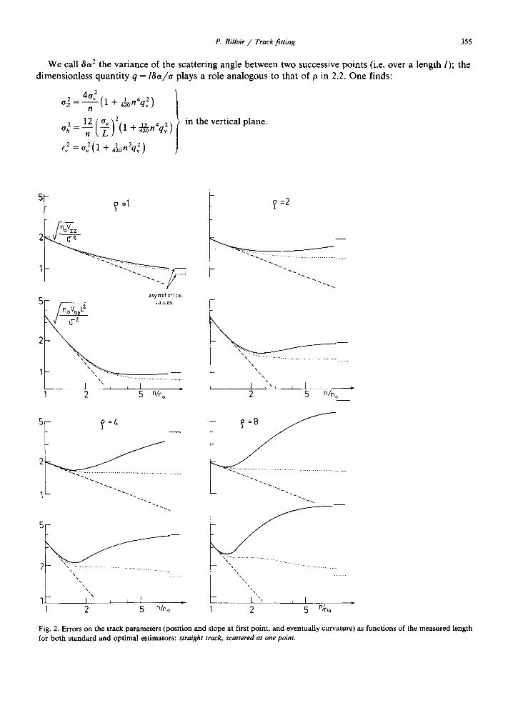
In these expressions the first term represents the well known contributions of the measurement errors. In order to show how the errors on the parameters depends on the measured length (i.e. the number of

points), figs. 2 and 3 (solid curves) represent the square roots of the variances (in normalized units) as function of n / n o for various values of 0: this quantity expresses the relative importance of the scattering errors for a given track/detector configuration; under usual experimental conditions, it can be much greater than 1 for particles with momentum around 1 GeV/c.

These curves often have an absolute minimum (and sometimes also a secondary minimum): so we are led to the notion of optimal measurement length: using points beyond this length worsens the precision of the estimator. Unfortunately the optimal length is generally not the same for all parameters;:in many cases the best precision for the curvature is obtained by using all measurements.

It is important to note that the mean squared residual r 2 is not affected in the same way by the scattering errors: one finds, for large n:

[1 + (n - 1)___3 02 in the vertical d Ov plane [ 3714 no

r~ - - -o~[ l+ (~-1)3(4~/~_ -12~ 615~+15) 02 ] n0] in the horizontal plane.

So the relative increase of the residuals due to the multiple scattering is generally much smaller that the increase of the variances of the fitted parameters. This implies that the X 2 criterion applied to the residuals fails to indicate whether the standard estimator is reliable in spite of the scattering.

When the particles encounter several slices of matter inside the measurement range, the successive scattering angles are independent: so the variances and the mean squared residuals can be calculated by adding the contribution of each slice.

2.3. Scattering uniformly distributed along the track

This approximation is exact for bubble chambers and realistic for many detectors. The variance of the parameters and the mean squared residuals are deduced from the formulae found in 2.2, with an integration over L 0 (as above, the number n of measurement points is assumed to be large enough to allow this approximation).


We call 8a 2 the variance of the scattering angle between two successive points (i.e. over a length l); the dimensionless quantity q = lra/o plays a role analogous to that of p in 2.2. One finds:

°2=4°2(ln_~ I n + 4~n4q2) 42) / gl+ nthoverti a,p,aoo.

a b ~- ~ n qv

1 3 2 rv 2 = a ~ ( 1 + ~ n qv ) }

=I

a s y m p f o t i c a l

- r vaLues - /_noVbbL~"

\ \ ' " ~

1_ , , I . 2 5 n/no

~,=2

x

\ x

x

\ \ \

2 5 n/no

5- ~,=t,

p

2 - - ".... ............................................................

x x .. . . . . .

x

- - \

q I ~ I I . 2 5 n/n o

\

x . . . . . . .

2 5 %o

Fig. 2. Errors on the track parameters (position and slope at first point, and eventually curvature) as functions of the measured length for both standard and optimal estimators: straight track, scattered at one point.

asymptotIcal

+--- I . ’ 2 5 n/n,

Fig. 3. Errors on the track parameters, as in fig. 2 but for: curved track, scattered at onepoinr.


o.,K/vb,~, q=o.ol

oo, I- \ \ "~..7 .......................................

0 . 0 2 [ - \ \ \

0.!

0.1 2 5 n(q

\,//~-cc.P q =0.04

0.02

0.01 ' \ o.oo~:- ' ~

o¢

0.I_ \ .............................................. ,,, ~ .. / ......

I I I 5 10 15 n(q ~-

Fig. 4. Errors on the track parameters, as in fig. 2 but for: straight track with uniformly distributed scattering.

Fig. 5. Errors on the track parameters, as in fig. 2 but for: curved track with uniformly distributed scattering.

__ 1 _4_2 9 o~(1 + s-Z~n qh) 0 " 2 ~ n

o ~ = -~- (1 +~-~n qh ) in the horizontal plane.

o 2 = ~ - ( ° h ]2( l+5-~n4q2 ) F/ r ~ = o ~ ( 1 - ' ~2 + ~-6n qh )

The dependence of ~z_, o b, o r . . . . on n (with l fixed) is shown in figs. 4 and 5: the errors have a min imum (at n = 3 .2 /~qv for o z and o b, at n = 6 . 8 / q ~ h for o v and %) excepted %, which decreases to zero. As a conclusion no opt imal length can be found to minimize the errors on all parameters simultaneously.

Here again the residuals are generally much less affected by the multiple scattering than the errors on the parameters (as a matter of fact, r 2 increases a s n 3 instead of n 4 for the variances); in most cases they reflect the measurement errors only.

3. T h e opt imal fit: recurs ive m e t h o d

3.1. Description of the method

3.1.1. General features The track is measured at abscissas x 1, x z . . . x N. Knowing the best estimators of the track parameters at

358 P. Bdlo ir / T rack f i t t ing

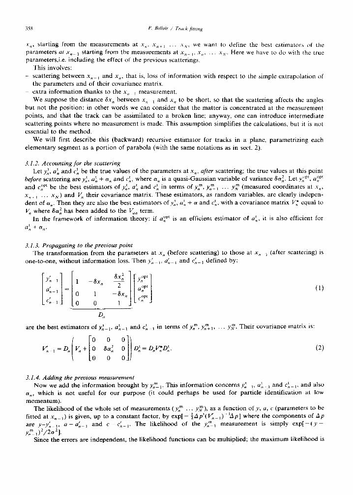
x,,, s tar t ing from the measurements at x . , x,,+~ . . . . xx, we want to def ine the best es t imators of the pa rame te r s at x~_~ s tar t ing f rom the measurement s at x . . . ~, x,,, . . . x x. Here we have to do with the true parameters , i .e , inc luding the effect of the previous scatterings.

This involves:

- scat ter ing between x . _ ~ and x . , that is, loss of in fo rmat ion with respect to the s imple ex t rapo la t ion of the pa rame te r s and of their covar iance matrix.

- ext ra in fo rma t ion thanks to the x n._ ~ measurement . We suppose the d i s tance 6x . between x,, ~ and x . to be short , so that the scat ter ing affects the angles

bu t not the pos i t ion: in o ther words we can cons ider that the ma t t e r is concen t ra t ed at the measurement points , and that the t rack can be ass imi la ted to a b roken line; anyway, one can in t roduce in te rmedia te scat ter ing po in ts where no measuremen t is made. This a s sumpt ion s implif ies the calculat ions, but it is not essential to the method.

W e will first descr ibe this (backward) recursive es t ima tor for t racks in a plane, pa ramet r i z ing each e l emen ta ry segment as a po r t ion of p a r a b o l a (with the same no ta t ions as in sect. 2).

3.1.2. Accounting for the scattering Let yt , a t and ct. be the true values of the pa rame te r s at x . , after scat ter ing; the true values at this po in t

vopt opt t + a . and ct., where a . is a quas i -Gauss i an var iable of var iance 3a] . Let ~n , a~ before scat ter ing are yt , a . t and t in terms of ym, y . + ~ YN (measured coord ina tes at xn, and c . opt be the bes t es t imators of yt , a . c. m . . . rn

x.+~ . . . x N) and V. their covar iance matr ix. These es t imators , as r a n d o m variables , are clearly independen t of a . . Then they are also the best es t imators of.v t , a t + a and ct., with a covar iance matr ix V.* equal to

V. where 3a~ z has been a d d e d to the V.. term. t it is also efficient for opt is an eff icient e s t ima tor of a . , In the f r amework of in fo rma t ion theory: if a .

t +Otn" a n

3.1.3. Propagating to the previous point The t r ans fo rma t ion f rom the pa rame te r s at x , (before scat ter ing) to those at x n ~ (af ter scat ter ing) is

one- to-one , wi thout in fo rma t ion loss. Then y~,. ~, a~, t and c~,_ ~ def ined by:

2 / an°pt 1 - 3 x . [c , ,p, 0 1

Y!- 1

a~_ = 0 cn- 0

are the best es t imators of y t_ 1, a tn-I and cn-~t in terms of ym, Y,~ 1, . .. y ~ . Thei r covar iance matr ix is:

v . _ l = D. V. + 8~. D'. = D.~D.' , .

0

(1)

(2)

3.1.4. Adding the previous measurement N o w we add the in fo rma t ion b rought by yff_ 1. This in fo rma t ion concerns y t_ 1, a t . - 1 and c~, ~, and also

an, which is not useful for our pu rpose (it could pe rhaps be used for par t ic le ident i f ica t ion at low

m om en tum) . The l ike l ihood of the whole set of measurement s (ym . . . yQ) , as a funct ion of y, a, c (pa ramete rs to be

f i t ted at x . _ t) is given, up to a cons tan t factor, by e x p [ - ½Apt(If n_ l ) - tAP] where the c ompone n t s of zap are Y-Y' . -1 , a - a'~_ 1 and c - e ; , _ i. The l ike l ihood of the ym_ 1 measuremen t is s imply e x p [ - ( y - ym_,)2/2o2] .

Since the errors are independen t , the l ike l ihood funct ions can be mul t ip l ied ; the m a x i m u m l ike l ihood is

P. Billoir / Track f i t t ing 359

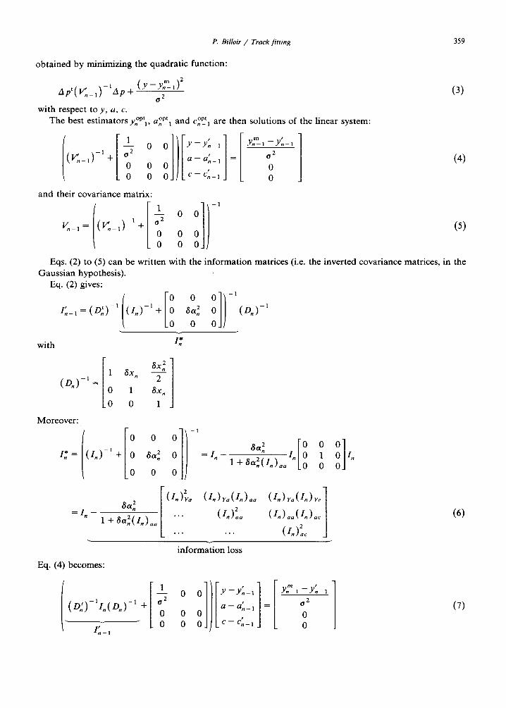
obta ined by minimizing the quadrat ic function:

m )2 (Y - Y . - 1 A p t ( -1 v' ._,) a p + 2

O with respect to y, a, c.

The best es t imators y°_pt 1, a °vt and c °pt . - a n-1 are then solutions of the linear system:

1 0 1 [ _ _ " ynm_l--Y'n_l (I.'._,)-'+ ~ 0 0 Y Y~-' 0 2

- - a n _ 1 0 0 , 0 0 0 - c~-l 0

and their covar iance matr ix:

1

v~_,= (~ ._ , ) - ' + 0 0 o° 1/0 o

(3)

(4)

(5)

Eqs. (2) to (5) can be wri t ten with the in format ion matr ices (i.e. the inverted covar iance matrices, in the Gauss ian hypothesis) .

Eq. (2) gives: 0 0]) I~,_, = ( D r ) -1 ( I , , ) - ' + 8a] 0 (D , , ) -1

0 0

with

( O . ) - ' =

0

Moreover :

1.*= (I,,)- '

= / . -

8z~. 1 8x n 2

0 1 8x. 0 1

[ -0 0 0 -

+ 0 ~a2

0 0

~a 2 [ ( In )2a

1 + 80t2(I,,),,,, "'"

= / . - ~,,~ [o 0 o]

2 / . /o 1 0J.t. 1+8, . . ( / . )o, , [o o o

• .. (,.)L I

Eq. (4) becomes:

in format ion loss

(6)

1 -1 (D.')- I . (D . ) +

I ' _ 1

1 o

0 0 0 0

o]l[y , o///o a,., OJ]tC-C.-,

m t Y,;-a --Yn-1

= 0 2 0 0

(7)

360 P. Billoir / T r a c k f i t t ing

and eq. (5) gives:

' oO] I~_,=I'~ ,+ oS 0 0 .

0 0 0 0

information brought by the measurement

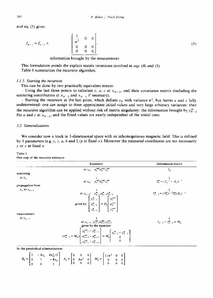
This formulation avoids the explicit matrix inversions involved in eqs. (4) and (5). Table 1 summarizes the recursive algorithm.

(s)

3.1.5. S t a r t i n g the recurs ion

This can be done by two practically equivalent means: - Using the last three points to calculate y, a, c at Xs_ 2, and their covariance matrix (including the

scattering contribution at x s _ 2 and x N_ 1 if necessary). - Starting the recursion at the last point, which defines YN with variance 0 2, but leaves a and c fully

undetermined: one can assign to them approximate initial values and very large arbitrary variances: then

the recursive algorithm can be applied without risk of matrix singularity: the information brought by y~_ 2 fits a and c at x s _ 2, and the fitted values are nearly independent of the initial ones.

3.2. G e n e r a l i z a t i o n s

We consider now a track in 3-dimensional space with an inhomogeneous magnetic field. This is defined by 5 parameters (e.g. y, z, a, b and 1 / p at fixed x) . Moreover the measured coordinates are not necessarily y or z at fixed x.

Table 1 One step of the recursive estimator

Estimator Information matrix

at x,,: yn°Pta°nPtc°n pt I .

at x.: yn°Pta°nPtc°Pt 1"~ = ( I.,-1 + A . ) 1

atx._~: y*.-:*.-,C-, 1.* ~=~D.~)-'I.*¢D.)

[:'1 given by: [a*_ 1 = ~ . / a : ' /

~:-, L c;., j

scattering at x .

propagation from

X n t O X n _ 1

measurement at x . _ ,

• o p t o p t o p t a t x n - - l . Yn-- l a n - - lCn--1

given by the equation: r:,:] "*._, + M.)|a°"_' , - aX_, = M . [ o

L c°"-', - c*._,

= * M n In - I 1._ I +

In the parabolical schematization:

I00 I0 1 - 8x. 8 x Z . / 2 "0

D . = 1 - 8 x n An =

0 1

0il [,,o201] 8 a 2 M,, = 0 "

0 0


We describe hereafter the 3 stages of each step of the recursion. Instead of the aximuth ~ and the dip ~,, we continue to us the slope parameters a =Py/Px = tan ~ and b =pJp~ = tan )~/cos ~: this avoids trigonometrical calculations. We use also: d = Ze /p (B . d is then the curvature for a track perpendicular to the magnetic field).

3.2.1. scattering at x~ This affects only h and ~ (or a and b). Let ~n be the number of radiation lengths X 0 crossed from x n_ 1 to

x~. For a 'homogeneous medium:

x n - x ,_ 1 8x, x/1 + a2 + b2 (9) in = X0 cos X cos ~, = Xo

The scattering angles a and/~ in two perpendicular planes containing the track direction are independent random variables of variance 6a 2 = (KZ/pv)2~n. If one of these planes is vertical, the scattering angle in this plane represents exactly the variation of ~ and the other one of the variation of ~ multiplied by cos h; with the parameters g, and h, to account for the scattering consists in adding 8a2/cos22~ to V** and 8a2n to Vxx.

With the parameters a and b, one finds easily, that one has to add:

oOoo oOl)-, (In) -1 + ~,~ ~---~ 0 ,

i a l 0 t . _ _ _ , d

0 0 0

( l + a 2 + b 2 ) ( 1 + a 2 ) S a ~ to V~

( l + a 2 + b 2 ) ( 1 + b 2)8a~ to Vbb

( l + a 2 + b 2 ) a b 8a 2 to Vab.

In terms of information matrices, we get:

0 0 0 0

i* = ( ~ ) - ' ffi o o

0 0 0 0

A = ( l + a 2 + b 2 ) [ l + a 2 ab ] ab 1 + b E "

where

(10)

(11)

The matrix inversions can be simplified in the same way as in sect. 3.1.4.:

0 0 0 0 O ] 0 0 0 0 0

~ * = ~ - 8 ~ I ~ o o r . . . . ~, o ~ ,

o o , ~ a ; o 0 0 0 0 0

(12)

with

.:(A l+ o ['ao '

3.2.2. Propagation from x~ to x~_ 1: The track extrapolation from a point to the previous one must be accurate: the cumulated error over the

362 P. Billoir / Track f i t t ing

whole length of the track should remain small with respect to the position uncertainty resulting from the fit. Any suitable method for this extrapolation allows to calculate also the (5 × 5) matrix of derivatives analogous to D, in eq. (1), either by analytical differentiation, or by finite differences.

As a matter of fact, on the left-hand side of the equation which should generalize eq. (4), the matrix ~,_ ~ can be calculated with an approximation for D~, assuming the field B to be constant along the track between x,,_ 1 and x, . If the curvature is not too strong, we obtain for the parameters y, z, a, b and d:

-1 0

0 1

Dn--- 0 0

0 0

0 0

2 - 3x,, + F~ 3x,,/2 F23x2.,/2 F33x2/2

G,3x2/2 -6x , , + G23x2/2 G33x2/2

1 - F13x,, - F 2 3 x n - G 3 x n

- G18x,, 1 - - G 2 6 x . - G 3 3 x .

0 0 1

(13)

with

F3=e[bB x + abBv- (1 + a2)Bz] ;

G3= e [ - a B x +(1 + b 2 ) B y - abBz];

F l = d [ a F 3 / e 2 + e ( b B v - 2 a B z ) ]

F2=d[bF3/e 2 + e ( B x + aBv) ]

G 1 = d[aG3/e 2 - e ( B x - bBz) ]

G 2 = d [ b G 3 / e 2 + e ( 2 b B y - a B z ) ] ,

w h e r e e 2 = 1 + a 2 + b 2.

3.2.3. Addition of a measurement In many cases each measurement consists in determining y or z, or a combination t = )~y +/~z, at a

given fixed x. Here it is useless to build space points from several raw measurements: such a procedure implies sometimes a loss of information.

The likehood of measurement t m is now, in the Gaussian approximation: n--1

1 (Xy +/~z_- t ._a) exp -

and the linear system (4) becomes:

Ill 1[ 1 #2 0 0 0 z - z . _ l , , . 1 ~ ' ( t T - , - X Y . - , - ~ ' z . - , ) (14)

0 0 0 0 a - a , , _ 1 = o S 0 (~n- ' ) - l - [ -~"~ 0 0 0 0 b - b ' [ o °_ , o

0 0 0 0 d - d' 0 n--1

Of course, if y and z (or two independent combinations of y and z) are available at the same x, both measurements can be included together in one equation like (14).

If the information refers to a non-linear combination of y and z, it can generally be linearized around the measured values.

When the measured quantity depends only on x, especially in the case of optical measurements, one can transform the raw information into information at fixed x; this transformation is a projection along the direction of the track. Several examples are described in detail in ref. [4].


3.3. Extension to energy loss

The energy loss can be taken into account in natural way: it is enough, in the progagation, in the propagation stage 3.2.2., to add a suitable quantity to the d parameter. Moreover, it is possible to introduce a (Gaussian) uncertainty on this energy loss, as in 3.2.1., by adding a contribution to Vad in the same time as V.~, Vh~ and V~b at the scattering stage.

4. Comparison between the optimal fit and the standard fit

4.1. Introduction

Our aim is to determine the gain in precision on the parameters, brought by the optimal estimators, with the same model as in 2.2. and 2.3., and the same notations.

In the optimal fit, the variances of the parameters cannot increase as measurement points are added (in other terms, addition of measurement cannot cause a loss of information). Thus, for n ~ ~ they must tend toward some limits (possibly zero). Again we use the Gaussian approximation: so the covariance matrix V of the fitted parameters is the inverse of the information matrix I.

4.2. Scattering at one point

The expressions of the measured variables show that the measurements after L 0 are independent of those before L0, so that the total information matrix on the parameters ( Z and b) at the origin is the sum of the contributions brought by the two portions of track delimited by the scatterer

For the second portion (after L0) , we calculate first the information on the parameters at x - - -L 0 (including the effect of the scattering uncertainty), and then we propagate it back to x -- 0. At x = 0 we add the information of the first portion (before L o), where no scattering uncertainty occurs.

This calculation gives the covariance matrix of the parameters, hence their errors as represented in fig. 2a and b (dotted curves). These curves show that the gain in precision of the optimal estimator is large when p is large a n d / o r when n > 3n o (however at very large values of n the gain vanishes for the curvature).

Let us note that in this case (scattering at only one point) the optimal fit can be reduced to two standard fits (one for each track portion, before and after Lo) connected together by the three elementary operations defined in sect. 3: accounting for the scattering at x = L 0 for the second portion, propagating the information matrix of this portion back to the first point, and adding the information of both portions. An analogous strategy could be adopted with few scattering points, provided that each portion of track between two scatterers has a sufficient number of points to perform a standard fit: the information brought by each portion could then be merged recursively as described in sect. 3.

4.3. Uniformly distributed scattering

The formalism developed in sect. 3 gives a recursive expression of the optimal information matrix: if the track has n + 1 points, the last n points give an information matrix I , for the parameters at the second point; then the first measurement can be added within one step of the recursion: so we obtain 1,+ 1 for the parameters at the first point.

For Z and b parameters (straight line fit in the vertical plane) this gives:

0]


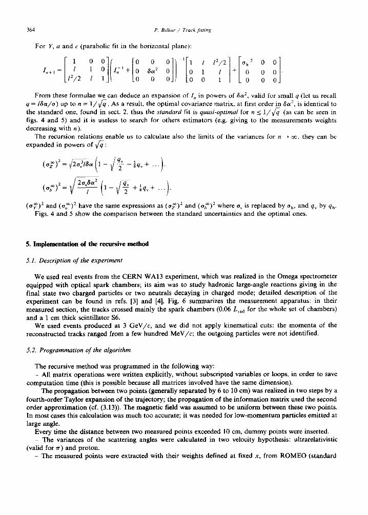
For Y, a and c (parabolic fit in the horizontal plane):

[, ° °If (i ° ill Ii ,,2j2 1 . + 1 = l 1 0 I n 1 + 3 a 2 1 l

12/2 l 1 0 0 1

Oh 2 0 0

+ 0 0 " 0 0

From these formulae we can deduce an expansion of I n in powers of 8a 2, valid for small q (let us recall q = lSa/o) up to n = 1 / ¢ q . As a result, the optimal covariance matrix, at first order in ~a 2, is identical to the standard one, found in sect. 2. thus the standard fit is quasi-optimal for n < 1/v/q (as can be seen in figs. 4 and 5) and it is useless to search for others estimators (e.g. giving to the measurements weights decreasing with n).

The recursion relations enable us to calculate also the limits of the variances for n --, oo. they can be expanded in powers of e q :

qv _ qv÷ ...).

Io;,2;¢ ) (~r~) 2 and (aa°°) 2 have the same expressions as ( o ~ ) 2 and ( o ~ ) 2 where o v is replaced by o h, and qv by qh.

Figs. 4 and 5 show the comparison between the standard uncertainties and the optimal ones.

5. I m p l e m e n t a t i o n o f t h e r e c u r s i v e m e t h o d

5.1. Description of the experiment

We used real events from the CERN WA13 experiment, which was realized in the Omega spectrometer equipped with optical spark chambers; its aim was to study hadronic large-angle reactions giving in the final state two charged particles or two neutrals decaying in charged mode; detailed description of the experiment can be found in refs. [3] and [4]. Fig. 6 summarizes the measurement apparatus: in their measured section, the tracks crossed mainly the spark chambers (0.06 Lra d for the whole set of chambers) and a 1 cm thick scintillator $6.

We used events produced at 3 GeV/ c , and we did not apply kinematical cuts: the momenta of the reconstructed tracks ranged from a few hundred MeV/c ; the outgoing particles were not identified.

5.2. Programmation of the algorithm

The recursive method was programmed in the following way: - All matrix operations were written explicitly, without subscripted variables or loops, in order to save

computat ion time (this is possible because all matrices involved have the same dimension). - The propagation between two points (generally separated by 6 to 10 cm) was realized in two steps by a

fourth-order Taylor expansion of the trajectory; the propagation of the information matrix used the second order approximation (cf. (3.13)). The magnetic field was assumed to be uniform between these two points. In most cases this calculation was much too accurate; it was needed for low-momentum particles emitted at large angle.

Every time the distance between two measured points exceeded 10 cm, dummy points were inserted. - The variances of the scattering angles were calculated in two velocity hypothesis: ultrarelativistic

(valid for or) and proton. - The measured points were extracted with their weights defined at fixed x, from ROMEO (standard


reconstruction program for Omega events), just before the final fit, so that both fitting procedures worked on exactly the same input.

- The starting value of the curvature parameter was estimated with three points (at the beginning, in the middle and at the end of the track); for the slope parameters, the last two points were used, with a curvature correction. As a matter of fact, the fitted values do not appear to depend strongly on the initial ones. After 3 or 4 recursion steps, the gaps between the extrapolated trajectory and the measured points are compatible with the measurements errors, and moderate deviations on the starting values are automatically corrected; for example, estimating the slope without curvature correction between the last two points has no appreciable effect on the fitted values.

The computation time for one recursion step (propagation + measurement + scattering) amounted to about 360/~s on CDC CYBER 750, equivalent to 160/~s on CDC 7600 (the computat ion of the magnetic field is not included). The time for a whole track is obviously proportional to the number of points on this track.

5.3. Test o f the precision

From the parameters fitted at the first measured point we extrapolated the tracks backwards to find intersections, and we determined the points of closest approach between each pair of tracks with opposite sign.

Fig. 7 shows the distributions of the minimal distances obtained with the standard program ROMEO, and with our algorithm (for both mass hypotheses).

200'

100, -• a) standard f i t (ROMEO}

L

beam

["

h , ,

__/iJI I

I optical modutes (spark chambers)

200-

I00-

200-

100 -

our method

hyp. rc for bo'th part icles

:_ J

--• c) our method

hyp. p /~ for both par t ic les

c , - - : 2 2 wire chambers ~ ~, scintitlaf0rs 1 2 cm

Fig. 6. Layout of the WA13 experiment in the Omega Spectrometer.

Fig. 7. Comparison between the standard fitting method of ROMEO and the re.cursive implementation of the optimal estimator: distance, at the point of closest approach, between two tracks extrapolated backwards to the vertex.


The precision is clearly improved by our method. The improvement is not very strong, but anyway the theoretical gain that we could deduce from sect. 4 for this experiment, is not enormous. Moreover there was matter accumulated around the vertex (the hydrogen target was surrounded by scintillators) which worsened its geometrical precision, and for which optimization cannot help. For the same reason, no appreciable improvement can be expected in the kinematical resolution.

6. C o n c l u s i o n

The standard fitting procedures, applied to slow tracks measured over a long length, a n d / o r with high accuracy, lead to important losses of precision on the geometrical parameters. They can be improved by taking account of the measurements up to a certain length only; this optimal length can be evaluated from analytical approximations of the variances. In many cases, especially in a homogeneous medium, this " t runcated" fit is not far from being optimal. Its main drawback is that the optimal length depends on the choice of parameter for which one wants the highest precision; moreover it was calculated assuming Gaussian independent measurement errors, and we do not know how it would be modified by small uncorrected geometrical distorsions, or by non-Gaussian errors (e.g. in a MWPC).

The optimal fit (without information loss) is usually realized by calculating the whole covariance matrix of the measurements, or by adding extra parameters to describe the scattering [1]; these methods involve handling big matrices. In this paper we described a new implementation of the optimal estimator: the parameters are fitted backwards by introducing the measured points one at a time from the end to the beginning of the track. The elementary steps are thus: including one or several raw measurements, a n d / o r one elementary scattering: from one point to the next one the parameters and their information (or weight) matrix are propagated by a local polynomial parametrization.

Such a procedure is very flexible: it can be applied to various types of detectors, and especially to composite detectors. Moreover it does not require more computation time than the standard ones (perhaps less); contrary to the "b ig matrix" optimal methods, the time used is merely proportional to the number of points.

The implementation of this algorithm on real events shows an improvement of the geometrical accuracy; its order of magnitude corresponds to what could be expected. The fitted values of the parameters appear to be stable with respect to the starting value chosen at the end of the track: thus no iteration is needed to obtain the best estimate; the algorithm stabilizes after 3 or 4 steps along the track.

Finally we point out that this method, in some configurations, could be able to perform at the same time the pattern recognition and the geometrical reconstruction of the tracks, since it gives in a short time the best extrapolation of a track candidate built up with the most external points.

I thank Professor M. Froissart for helpful discussions and suggestions.

R e f e r e n c e s

[1] H. Eichmger and M. Regler, CERN 81-06, Review of track-fitting methods in counter e×periments. [2] D. Drijard, CERN/D.Ph. II/Prog. 69-4, Handfing of multiple scattering in track reconstruction. [3] R. Schwarz, Thesis, Neuch~ttel (1982). [4] P. BiUoir, Thesis, Paris VI (1983).

track fi'iting with multiple scaitering: a new...

Documents