TOA-Based Robust Wireless Geolocation and

Cramér-Rao Lower Bound Analysis in Harsh

LOS/NLOS Environments

Feng Yin, Carsten Fritsche, Fredrik Gustafsson and Abdelhak M Zoubir

Linköping University Post Print

N.B.: When citing this work, cite the original article.

©2013 IEEE. Personal use of this material is permitted. However, permission to

reprint/republish this material for advertising or promotional purposes or for creating new

collective works for resale or redistribution to servers or lists, or to reuse any copyrighted

component of this work in other works must be obtained from the IEEE.

Feng Yin, Carsten Fritsche, Fredrik Gustafsson and Abdelhak M Zoubir, TOA-Based Robust

Wireless Geolocation and Cramér-Rao Lower Bound Analysis in Harsh LOS/NLOS

Environments, 2013, IEEE Transactions on Signal Processing, (61), 9, 2243-2255.

http://dx.doi.org/10.1109/TSP.2013.2251341

Postprint available at: Linköping University Electronic Press

http://urn.kb.se/resolve?urn=urn:nbn:se:liu:diva-92694

1

TOA Based Robust Wireless Geolocation and

Cramer-Rao Lower Bound Analysis in Harsh

LOS/NLOS EnvironmentsFeng Yin, Student Member, IEEE, Carsten Fritsche, Member, IEEE, Fredrik Gustafsson, Fellow, IEEE

and Abdelhak M. Zoubir, Fellow, IEEE

Abstract—We consider time-of-arrival based robust geoloca-tion in harsh line-of-sight/non-line-of-sight environments. Herein,we assume the probability density function (PDF) of the mea-surement error to be completely unknown and develop aniterative algorithm for robust position estimation. The iterativealgorithm alternates between a PDF estimation step, whichapproximates the exact measurement error PDF (albeit unknown)under the current parameter estimate via adaptive kernel densityestimation, and a parameter estimation step, which resolves aposition estimate from the approximate log-likelihood functionvia a quasi-Newton method. Unless the convergence conditionis satisfied, the resolved position estimate is then used to refinethe PDF estimation in the next iteration. We also present thebest achievable geolocation accuracy in terms of the Cramer-Rao lower bound. Various simulations have been conducted inboth real-world and simulated scenarios. When the number ofreceived range measurements is large, the new proposed positionestimator attains the performance of the maximum likelihoodestimator (MLE). When the number of range measurements issmall, it deviates from the MLE, but still outperforms severalsalient robust estimators in terms of geolocation accuracy, whichcomes at the cost of higher computational complexity.

Index Terms—Adaptive kernel density estimation (AKDE),Cramer-Rao lower bound (CRLB), non-line-of-sight (NLOS)mitigation, robust geolocation, time-of-arrival (TOA).

I. INTRODUCTION

Wireless geolocation refers to the problem of finding the

position of a mobile subscriber in different wireless systems,

such as cellular networks, wireless local area networks, and

wireless sensor networks [1]. Over the past two decades,

wireless geolocation has received considerable attention due

to the expanding location-based services, such as wireless

Emergency 911 (E-911) service, location-sensitive billing,

fraud detection, intelligent transportation systems and mobile

yellow pages [2]. In order to give a position estimate, most

geolocation systems utilize a two-step geolocation technique

Copyright c©2012 IEEE. Personal use of this material is permitted. How-ever, permission to use this material for any other purposes must be obtainedfrom the IEEE by sending a request to pubs-permissions@ieee.org.

F. Yin and A. M. Zoubir are with the Signal Processing Group, Instituteof Telecommunications, Technische Universitat Darmstadt, Darmstadt, 64283,Germany (e-mail: fyin@spg.tu-darmstadt.de; zoubir@spg.tu-darmstadt.de).

C. Fritsche was with the Department of Electrical Engineering, Divisionof Automatic Control, Linkoping University, Linkoping, SE-581 83, Swe-den. He is now with the IFEN GmbH, Poing, 85586, Germany (e-mail:carsten@isy.liu.se).

F. Gustafsson is with the Department of Electrical Engineering, Divisionof Automatic Control, Linkoping University, Linkoping, SE-581 83, Sweden(e-mail: fredrik@isy.liu.se).

primarily due to its lower complexity as compared to a direct

geolocation technique (see e.g., [3], [4]). In the first step of the

two-step geolocation technique, position related measurements

such as received-signal-strength (RSS), time-of-arrival (TOA),

time-difference-of-arrival (TDOA) and angle-of-arrival (AOA)

are extracted. In the second step, the obtained measurements

are processed so as to give a position estimate. Various

different position estimation approaches can be found in [5]–

[8] and references therein.

In indoor environments or urban areas, non-line-of-sight

(NLOS) propagation significantly degrades the estimation per-

formance of conventional position estimation techniques (e.g.,

[9]–[14]), which are developed solely under the line-of-sight

(LOS) assumption. Therefore, robust methods for position

estimation are constantly sought after. In this paper, we focus

on the design of a new robust position estimation approach

based on the extracted TOA measurements. The existing TOA

based robust position estimation approaches can be broadly

categorized into “identify and discard” based approaches,

“mathematical programming” based approaches and robust

estimation based approaches.

The essence of the “identify and discard” based approaches

(see e.g., [15]–[17]) is to identify and discard those NLOS-

corrupted range measurements. The remaining range mea-

surements, classified as LOS measurements, are then used

by conventional algorithms (e.g., least-squares and maximum

likelihood algorithms) to compute an accurate position esti-

mate. The key idea of “mathematical programming” based

approaches is to formulate the position estimation problem

as a constraint optimization problem, which can be solved

by mathematical programming techniques (e.g., quadratic pro-

gramming [18], linear programming [19], and semi-definite

programming [20]). In order to combat the NLOS effect,

robust estimation based approaches resort to replace the least-

squares residual formulation by a robust statistics based on

[21], [22]. In the literature, the term “residual formulation” is

often regarded as a synonym for the term “score function”. In

[23], [24], robust least-median-squares based approaches were

proposed. In [25], a robust bootstrapping M-estimation ap-

proach that combines Huber’s M-estimation and the bootstrap

[26]–[28] was proposed. For further improvement, an adaptive

approach that tunes Huber’s score function was introduced in

[29], [30]. Most of the aforementioned approaches as well as

many other robust position estimation approaches can be found

in [31].

2

In harsh situations, where NLOS propagation dominates,

i.e., a majority of the measurements are outliers, and the

probability density function (PDF) of the measurement error is

completely unknown, robust position estimation becomes ex-

traordinarily challenging. To the best of our knowledge, those

approaches from the first and second categories are not able

to work properly under unknown measurement errors. Even

if some prior knowledge about the measurement error can be

obtained in a training stage, the high computational complexity

of these approaches is the main drawback for their practical

use. Robust estimation based approaches are favorable in harsh

situations, while classical approaches are merely robust for

up to 50% of outliers. In order to achieve more robustness

against the NLOS effect, two new fashioned robust estimation

approaches have been proposed in [30] and [32] respectively.

The gist of the two approaches is to approximate the maximum

likelihood estimator (MLE). By following the same design

philosophy, we propose in this paper a new robust position

estimation approach, which outperforms the existing robust

approaches by far.

Our original contributions of this paper are summarized as

follows:

• We propose an iterative geolocation algorithm, which

alternates between a PDF estimation step and a position

estimation step. Starting with a carefully selected initial

position estimate, we construct an estimate of the exact

measurement error PDF via adaptive kernel density esti-

mation (AKDE) [33], and then formulate an approximate

log-likelihood function, from which a refined position

estimate is resolved via a quasi-Newton method.

• We present the best achievable geolocation accuracy

in terms of Cramer-Rao lower bound (CRLB), which

serves as a benchmark for comparison of different robust

position estimators.

• We demonstrate the performance of the proposed algo-

rithm in a real-world scenario in Germany. The simulation

results show that the proposed algorithm outperforms its

competitors by far and behaves nearly optimally for a

large sample size.

• We exemplify several practically relevant signal pro-

cessing applications, to which our algorithm design and

CRLB analysis can be directly applied.

The remainder of this paper is organized as follows: In

Section II, we introduce the signal model and state the problem

at hand. In Section III, we briefly review the robust position

estimation approach in [30], followed by our new algorithm.

In Section IV, adaptive kernel density estimation is introduced.

Theoretical performance analysis is performed in Section V,

followed by simulation results which are obtained based on

a real-world scenario in Section VI. Finally, Section VII

concludes this paper.

II. SIGNAL MODEL

Consider the scenario where N(N ≥ 3) base stations (BSs)

surround a stationary mobile station (MS) of interest in a

wireless cellular network. Let [xi, yi]T denote the a priori

known geographic coordinates of the ith BS, i = 1, 2, ..., N

and let θ = [x, y]T denote the unknown coordinates of the MS,

where the superscript T stands for transpose. For each BS,

we obtain K(K ≥ 1) range measurement(s) and subsequently

relay them to a central site for post-processing [2].

Similar to [17], single path (LOS or NLOS) one-way propa-

gation is considered. Assuming a precise time synchronization

between the BSs and MS, we can express the kth range

measurement ri(k) measured at the ith BS by

ri(k) =√

(x− xi)2 + (y − yi)2︸ ︷︷ ︸

hi(θ)

+vi(k), (1)

k = 1, 2, ...,K , where hi(θ) represents the Euclidean distance

between the MS and the ith BS.1 The measurement errors

vi(k) are assumed to be independent and identically distributed

(i.i.d.) random variables whose PDF is completely unknown

to us. In the literature, the measurement error is often reported

to have a two-mode mixture PDF which can be written here

in a general form as follows:

pV (v) = (1− ε)N (v; 0, σ2L) + εH(v), (2)

meaning that a random variable v is N (v; 0, σ2L) distributed

with probability (1− ε) in a LOS environment or distributed

as H(v) with probability ε in an NLOS environment. Here,

ε is referred to as NLOS contamination ratio that quantifies

the impact of the NLOS effect, and N (v; 0, σ2L) represents

the Gaussian distribution with zero mean and variance σ2L.

In general, H(v) has a positive bias and a variance larger

than σ2L [6]. It is frequently modeled by a shifted Gaussian

distributionN (v; µNL, σ2NL) (e.g., in [6], [30], [32], [34]–[38]),

a Rayleigh distribution R(v) (e.g., in [30], [32], [39], [40]),

or an exponential distribution E(v) (e.g., in [30], [41], [42]),

depending on the actual scenario for geolocation. Note that we

motivate here the use of the two-mode mixture density model

that is often used in a variety of experimentations conducted

in mixed LOS/NLOS environments. We stress, however, that

the geolocation algorithm we design in the sequel does not

assume any model for the measurement errors.

For better readability, we express the signal model in a

compact vector form, yielding

r = h(θ) + v, (3)

where

r = [r1(1), . . . , r1(K), . . . , rN (1), . . . , rN (K)]T ,

h(θ) = [h1(θ), . . . , h1(θ)︸ ︷︷ ︸

K

, . . . , hN (θ), . . . , hN(θ)︸ ︷︷ ︸

K

]T ,

v = [v1(1), . . . , v1(K), . . . , vN (1), . . . , vN (K)]T .

Column vectors r, h(θ) and v are all of dimension NK × 1.

In the sequel, rm, hm and vm represent the mth element of

r, h(θ) and v respectively, with m = 1, 2, . . . , NK .

Our task is to estimate the MS position θ based on the

available set of range measurements r. In contrast to the vast

majority of papers available from the literature, we assume

that the noise density pV (v) is completely unknown.

1Range measurement and the corresponding TOA measurement only differby a constant scaling factor, namely the speed of light in a given medium.

3

III. ROBUST POSITION ESTIMATION

For the case that the PDF of the measurement error is

completely known, the MLE can be obtained by maximizing

the exact log-likelihood function, i.e.,

θMLE = argmaxθ

N∑

i=1

K∑

k=1

log pV (ri(k)− hi(θ))

= argmaxθ

NK∑

m=1

log pV (rm − hm) (4)

where log(·) denotes the natural logarithm operator for sim-

plicity.

The performance of estimators that rely on maximizing the

exact log-likelihood function generally degrades once the true

measurement errors deviate from the error model assumption.

Since the PDF of the measurement error pV (v) is assumed

completely unknown here, finding a robust position estimator

whose performance is close to that of the MLE given in (4)

is extremely challenging.

The idea we follow in this paper is to jointly combine posi-

tion estimation with PDF estimation in an iterative process.

According to the defintion in [43], the resulting parameter

estimation approaches fall in the class of semi-parametric

approach when the PDF pV (v) is estimated nonparametri-

cally and the vector parameter θ to be determined is of

finite dimension. The semi-parametric approach, which was

initially proposed for robust multiuser detection in impulsive

noise channels in [44], has its merits in dealing with the

problem where the noise PDF is unknown. In the context of

geolocation, however, the design of semi-parametric position

estimation approach is more challenging due to the nonlinear

signal model in general (e.g., (3) for TOA measurements).

Before proceeding with the new approach, however, we first

briefly revisit an existing semi-parametric approach for robust

position estimation, which was presented in [30].

A. Existing Robust Semi-Parametric Approach

In [30], the nonlinear signal model is first linearized by

squaring both sides of (1) as follows:

r2i (k) = h2i (θ) + v2i (k) + 2hi(θ) · vi(k)= Ri +R− 2xi · x− 2yi · y + vi(k), (5)

where

R = x2 + y2, (6)

Ri = x2i + y2i , (7)

vi(k) = v2i (k) + 2hi(θ) · vi(k). (8)

Reformulating (5) yields

r2i (k)−Ri = −2xi · x− 2yi · y +R + vi(k). (9)

Stacking all the terms in a vector, a linear regression model

is thus obtained, that is

r = Sθ + v (10)

with the vector notations defined by

r =

r21(1)−R1

...

r21(K)−R1

...

r2N (1)−RN

...

r2N (K)−RN

, S =

−2x1, −2y1, 1...

−2x1, −2y1, 1...

−2xN , −2yN , 1...

−2xN , −2yN , 1

,

v = [v1(1), . . . , v1(K), . . . , vN (1), . . . , vN (K)]T and θ =[x, y,R]T . Note that r and v are both of dimension NK × 1and S is of dimension NK × 3. Assuming the elements in

v are i.i.d. random variables with PDF pV (v), although not

always true, the log-likelihood function can be expressed by

NK∑

m=1

log pV (rm − Smθ) (11)

where Sm denotes the mth row of matrix S.

Since pV (v) is in fact unknown, two conceptually similar

iterative algorithms (cf. [30, Table I]) are proposed to resolve

an approximate MLE of θ from

NK∑

m=1

STm · ϕ

(

rm − Smθ)

= 0 (12)

where the score function is defined by

ϕ(v) = −p′V(v)

pV (v)(13)

with pV (v) denoting the estimated PDF using transformation

kernel density estimation (TKDE) and p′V(v) denoting the first

order derivative of pV (v) with respect to v. Given an extracted

residual vector ˆv on one iteration, TKDE is carried out to give

an estimated PDF pV (v) in the following four steps:

1) Transform the extracted residual vector ˆv via a trans-

formation z = t(ˆv; ζ), where the parameter ζ steers the

shape of this transformation function.

2) Symmetrize the transformed residual vector by zs =[−zT , zT ]T .

3) Perform conventional kernel density estimation (KDE)

upon zs and consequently obtain an estimated PDF

pZ(z).4) Transform pZ(z) back to pV (v).

Note that the transformation parameter ζ has to be determined

in an optimization procedure prior to the TKDE. Details of the

TKDE and the selection of a proper transformation parameter

can be found in [30, Appendix A and B], respectively.

Although this semi-parametric approach has shown consid-

erable improvements in the estimation performance as com-

pared to several other salient competitors [30], some issues still

remain unsolved. First, an auxiliary parameter R is introduced,

but the constraint condition R = x2 + y2 is not incorporated

in the optimization process, which surely leads to a sub-

optimal solution. The technique proposed in [45] may serve as

a powerful tool for remedying this drawback. Secondly, after

the linearization, the elements vi(k) for i = 1, . . . , N and

4

k = 1, . . . ,K in v are no more identically distributed due to

the factor hi(θ) in the expression of vi(k). Thirdly, in [30],

a transformation of the original residual vector ˆv has to be

conducted but there is no well established rule underpinning

the selection of a parametric transformation function t(ˆv; ζ) as

well as an appropriate interval [ζL, ζU ] for optimizing ζ, which

are crucial to the PDF estimation. As illustrated in [30, Fig. 7],

a wrongly selected transformation parameter ζ may severely

degrade the geolocation accuracy. For sake of avoiding these

drawbacks, we propose a new approach below.

B. Proposed Approach

The newly proposed approach is also a semi-parametric

approach according to the definition in [43]. In order to

distinguish between the two semi-parametric approaches, we

refer to the new approach as “robust iterative nonparametric

(RIN) approach” with the term “nonparametric” indicating

the fact that the measurement error PDF pV (v) is estimated

nonparametrically, and follow the name “semi-parametric ap-

proach” for the existing approach in the remaining parts of

this paper.

The main features of the new approach as compared to

the existing semi-parametric approach in [30] are highlighted

as follows. Firstly, the proposed algorithm directly uses the

nonlinear signal model. As a consequence, evaluation of

the constraint condition R = x2 + y2 is avoided and the

elements in v are i.i.d..2 Secondly, TKDE is replaced by

nonparametric adaptive kernel density estimation (AKDE) to

obtain an estimate of the measurement error PDF. This has the

advantage that the parameters required for constructing a den-

sity estimator are now set adaptively and fully automatically

as compared to the TKDE. Thirdly, a quasi-Newton method is

employed to resolve a position estimate from the approximate

log-likelihood function, which is derived based on the a priori

calculated PDF estimate. The key steps of the RIN position

estimation approach are summarized in Algorithm 1.

It is noteworthy that,

• the initial estimate θ(0) is set by the first two entries of

the least-squares solution of (10), i.e., by [xLS, yLS]T of

θLS = [xLS, yLS, RLS]T = (ST

S)−1STr; (16)

• the approximated noise density p(j)V (v) is composed of a

sum of Gaussian kernels as follows

p(j)V (v) =

1

NK

NK∑

m=1

1√2πw(j)λ

(j)m

exp

[

− (v − v(j)m )2

2(w(j)λ(j)m )2

]

(17)

where v(j)m denotes the mth element of the residual

vector v(j); w(j) denotes the window width; and λ

(j)m ,

m = 1, 2, ..., NK denote the local bandwidth factors

calculated in the jth iteration;

2It is necessary to stress here again that we work with the nonlinear signalmodel in (3), where the entries in v are i.i.d., for the new algorithm designand CRLB analysis, while the existing semi-parametric approach [30] workswith the linearized signal model in (10), where the entries in v are not i.i.din general from our analysis.

Algorithm 1 Robust Iterative Nonparametric (RIN) Position

Estimation Approach

Step 1–Initialization: Define the convergence tolerance∆ and

the maximum number of iterations NmaxItr ; Set the iteration

index j = 0; Choose an initial guess θ(0) of the position

parameter θ to be determined.

Step 2–Perform Joint Estimation: In the jth (j ≥ 1)

iteration, sequentially do:

1) Determine the residual vector v(j) = r− h(θ(j−1)).2) Construct an estimate of the true probability density

function pV (v), p(j)V (v), from v

(j) via the nonparametric

AKDE described in Algorithm 3.

3) Approximate the exact log-likelihood function by

ll(j)(θ) =

N∑

i=1

K∑

k=1

log p(j)V (ri(k)− hi(θ)) . (14)

4) Define the negative of the approximate log-likelihood

function by g(j)(θ) = −ll(j)(θ) and update the position

estimate by minimizing g(j)(θ), more specifically,

θ(j) = argminθ

g(j)(θ), (15)

using (for instance) Algorithm 2.

Step 3–Convergence Check: If ‖θ(j) − θ(j−1)‖ < ∆ or

the maximum number of iterations NmaxItr is reached, then

we terminate the algorithm; otherwise we update the iteration

index j ← j + 1 and return to Step 2.

• the cost function g(j)(θ) is given by

g(j)(θ) = −N∑

i=1

K∑

k=1

log1

NK

NK∑

m=1

1√2πw(j)λ

(j)m

× exp

[

− (ri(k)− hi(θ)− v(j)m )2

2(w(j)λ(j)m )2

]

; (18)

• the operator ‖ · ‖ denotes the L2 norm.

Many numerical methods can be utilized to solve the

minimization problem formulated in (15), e.g., the Newton-

Raphson method [46], quasi-Newton method [47], and the

expectation maximization method [48]. Alternatively, it is

safest to perform a two-dimensional (2-D) grid search in the

vicinity of a good initial guess [49]. But the drawback lies

in the higher computational complexity. In this paper, we use

the Broyden-Fletcher-Goldfarb-Shanno (BFGS) quasi-Newton

method to minimize the nonlinear cost function g(θ), since

it guarantees downhill progress towards the local minimum

in each Newton step [50]. The key steps of the BFGS quasi-

Newton method are listed in Algorithm 2. It is noteworthy to

mention that the iteration index j of g(j)(θ) is discarded for

brevity in Algorithm 2.

The reasons that we choose the least-squares solution as

the initial value in Algorithm 1 are due to its simplicity and

rather low computational complexity [6]. However, in the case

where the least-squares solution may largely lose its accuracy,

we have to resort to a more sophisticated strategy in which we

use several candidate initial values and finally choose the one

5

leading to the maximal value of the approximate log-likelihood

ll(1)(θ) (cf.(14)) after the first iteration of Algorithm 1.3 The

disadvantage of such an approach is the increase in compu-

tational complexity. In the sequel, we merely test the least-

squares solution as the initial guess. In Section VI, simulations

confirm the performance of this simpler initialization strategy.

It is conspicuous from Algorithm 1 that the parametric

position estimation and the nonparametric PDF estimation

are tightly combined in an iteration process. Intuitively, the

improved position estimate will lead to a refined PDF estimate

and vice versa so that at the convergence of this iterative

algorithm a good estimation performance can be achieved.

However, it remains difficult, even asymptotically, to theoret-

ically analyze the performance difference between the new

position estimator and the corresponding MLE (cf. (4)) in

terms of bias and root mean squared error (RMSE). While

the MLE is known to be asymptotically efficient under some

regularity conditions, see [49, Theorem 7.3], this is not easy to

show for the new position estimator, due to the difficulties in

quantifying how well the true PDF pV (v) can be approximated

by its estimate pV (v) for a given number of observations.

But we still believe that the performance of the new position

estimator can be very close to that of the MLE when the

number of range measurements is sufficiently large. In this

paper, we evaluate the actual performance of the new position

estimator in a large-scale Monte Carlo simulation.

Algorithm 2 BFGS quasi-Newton method with a cubic line

search

1) Set l = 0 and obtain a search direction sl = −Hl ·∇θg(θl), where ∇θg(θl) is the gradient of the cost

function g(θ) evaluated at θl. The initial value θ0 is set

to θ(j−1) on the jth (j ≥ 1) iteration of Algorithm 1.

2) Find the step size αl along the direction sl via cubic line

search introduced in [51, Algorithm 3.5 and 3.6].

3) Update the estimate by θl+1 = θl + αlsl.

4) Set δl = αlsl and γl = ∇θg(θl+1)−∇θg(θl).5) Update the approximate Hessian matrix by

Hl+1 = Hl+(1+γTl Hlγl

δTl γl)δlδ

Tl

δTl γl−(δlγ

Tl Hl +Hlγlδ

Tl

δTl γl).

(19)

Note that, the initial approximate Hessian matrix H0 is

set to an identity matrix I2.

6) If ‖θl+1 − θl‖ < κ, then stop; otherwise update the

iteration index l← l + 1 and return to step 2.

IV. ADAPTIVE KERNEL DENSITY ESTIMATION

Kernel density estimation (KDE) is a nonparametric ap-

proach for estimating the PDF based on a given set of observa-

tions [33]. The key idea of KDE is to approximate the desired

PDF by a linear combination of kernel functions with carefully

3We can employ, for instance, the position estimates obtained from therobust M-estimation approach [29], [30] and the robust semi-parametricestimation approach [30] as well as the grid points in the vicinity of them.However, the computational cost highly depends on the total number of thegrid points.

chosen bandwidths. Amongst a large number of variations

of this kind, we employ here an adaptive kernel density

estimation approach, which gives overall good performance

in estimating a long-tailed and/or multi-modal PDF [33].

Assuming that we have a set of NK i.i.d. observations

v = {v1, v2, ..., vNK} generated from a continuous univariate

distribution with probability density function pV (v), the steps

required for constructing an adaptive kernel density estimator

pV (v) are demonstrated in Algorithm 3.

Algorithm 3 Adaptive Kernel Density Estimator

1) Find a pilot density estimator

p0(v) =1

NK

NK∑

m=1

1

w0G

(v − vmw0

)

(20)

where G(·) denotes a standard Gaussian kernel, w0 =0.79 · Iqr{v} · (NK)−1/5 denotes an initial global band-

width and Iqr{v} denotes the interquartile range of

v = {v1, v2, . . . , vNK}.2) Define local bandwidths λm, m = 1, 2, . . . , NK by

λm =

p0(vm)

/[NK∏

m=1

p0(vm)

] 1

NK

−β

(21)

where the sensitivity parameter β is set to 0.5 as sug-

gested in [52].

3) An adaptive kernel density estimator pV (v) is finally

constructed by

pV (v) =1

NK

NK∑

m=1

1

wλmG

(v − vmwλm

)

(22)

where the global bandwidth w is determined using the

least-squares cross-validation technique [33].

V. THEORETICAL PERFORMANCE METRICS FOR

GEOLOCATION ACCURACY

In this section, different performance metrics are presented

that can be used to assess the best achievable performance of

position estimators in harsh LOS/NLOS environments. Here,

it is worth noting that for the theoretical performance analysis,

pV (v) is assumed to be known.

A. Cramer-Rao Lower Bound

It is well known that the covariance matrix of any unbiased

estimator of an unknown vector parameter is lower bounded

by the Cramer-Rao lower bound [49], [17]. In the following,

CRLB analysis will be carried out based on our nonlinear

signal model in (3). Let θ = [x, y]T denote an unbiased

position estimator of a deterministic vector position parameter

θ = [x, y]T and let Cov(θ) denote the covariance matrix of θ.

Assuming that certain regularity conditions are fulfilled [53],

we have

Cov(θ) = Ep(r|θ)

{

(θ − θ)(θ − θ)T}

� F−1(θ) ≡ CRLB (23)

6

where F(θ) denotes Fisher information matrix (FIM), and

A � B means that the matrix difference A − B is positive

semidefinite. Let ∇θ = [∂/∂x, ∂/∂y]T denote the gradient

operator, and let ∆θ

θ= ∇θ∇T

θdenote the Laplace operator.

Then, FIM can be expressed as

F(θ) = Ep(r|θ)

{−∆θ

θ log p(r | θ)}

(24)

where the expectation is taken with respect to p(r | θ), namely

the PDF of r parameterized in θ. For nonlinear models with

non-Gaussian error v in (3), closed-form expressions for FIM

are generally not available. Here, Monte Carlo integration

techniques [54] can be used to numerically approximate the

expectation given in (24). Instead of performing Monte Carlo

integration directly on (24), we suggest the following proce-

dure. Often, it is more convenient to express FIM as follows

F(θ) = Ep(r|θ)

{∇θp(r | θ)∇Tθp(r | θ)

p(r | θ)2}

. (25)

It was shown in [55], [56] that for nonlinear models given by

(3), FIM in (25) can be reformulated as

F(θ) = H(θ) · Iv ·HT (θ) (26)

where

H(θ) = ∇θh(θ)

=

x− x1h1(θ)

, · · · , x− x1h1(θ)

︸ ︷︷ ︸

Krepetitions

, · · · , x− xNhN (θ)

, · · · , x− xNhN (θ)

︸ ︷︷ ︸

Krepetitions

y − y1h1(θ)

, · · · , y − y1h1(θ)

︸ ︷︷ ︸

Krepetitions

, · · · , y − yNhN (θ)

, · · · , y − yNhN(θ)

︸ ︷︷ ︸

Krepetitions

(27)

and

Iv = Epv(v)

{

[∇vpv(v)] · [∇vpv(v)]T

[pv(v)]2

}

. (28)

In Appendix A, it is proven that as long as the elements in v

are i.i.d., the matrix Iv is a diagonal matrix of the form

Iv = Iv · INK (29)

where INK is an identity matrix of dimension NK × NK ,

and Iv is calculated by

Iv = EpV (v)

{

[∇vpV (v)]2

p2V (v)

}

=

∫[∇vpV (v)]

2

p2V (v)pV (v)dv (30)

and referred to as intrinsic accuracy [57]. For most of the

measurement error distributions, it is difficult to derive Iv in

closed form. A notable exception, however, is the Gaussian

distribution N (v;µv, σ2v) and in this case Iv = σ−2

v . In the

other cases, the integral in (30) can be approximated using

Monte Carlo integration [54], yielding

Iv ≈1

NC

NC∑

n=1

[∇vpV (v

(n))]2

p2V (v(n))

(31)

where v(n), n = 1, 2, ..., NC are NC i.i.d. samples generated

from pV (v). It is obvious from (29) that for a specified pV (v),only one Monte Carlo integration has to be performed to

compute Iv if the elements in the vector v are i.i.d., and this

Iv can be used to compute the CRLB for several different

MS positions. This comes with a considerable reduction in

computational complexity as compared to performing Monte

Carlo integration directly on (25).

B. Bias and Root Mean Squared Error

In geolocation applications, it is desirable to design an

unbiased estimator with RMSE as small as possible [58]. The

bias of a position estimator is defined here by

Bias(θ) = Ep(r|θ){θ} − θ (32)

and the RMSE, frequently interpreted as the geolocation

accuracy of a position estimator, is related to the obtained

CRLB through

RMSE ≡√

Ep(r|θ){(x− x)2 + (y − y)2}

=

√

tr(

Cov(θ))

≥√

tr(F

−1(θ))≡ CRLBpos (33)

where tr (·) denotes the trace of a matrix, and CRLBpos can

be interpreted as the best achievable RMSE of an unbiased

position estimator.

C. Estimation Efficiency

Here, it is more convenient to re-define the efficiency of an

unbiased position estimator by

η =CRLBpos

RMSE=

√√√√

tr(F

−1(θ))

tr(

Cov(θ)) . (34)

It follows from (33) that 0 ≤ η ≤ 1. If a position estimator is

unbiased and simultaneously attains η = 1, then it is referred

to as an efficient position estimator. As it is well known, the

MLE obtained from (4) is asymptotically efficient—unbiased

and η = 1—as the number of measurements goes to infinity.

D. Geometric Dilution of Precision

Another important metric is called geometric dilution of pre-

cision (GDOP), which is used to describe the influence of BSs-

MS geometry on the relationship between the measurement

error and geolocation accuracy [59]. Since we have assumed

identical variance of the measurement errors at different BSs,

GDOP is easily calculated by

GDOP =

√√√√ tr

(

Cov(θ))

σ2v

(35)

where σ2v denotes the variance of the measurement error PDF,

pV (v). For an efficient position estimator, (35) becomes

GDOP =CRLBpos

σv. (36)

It was reported in [31] that GDOP values smaller than three

imply well-suited geometry, whereas those larger than six

imply a deficient geometry.

7

TABLE ISIMULATION PARAMETERS

Parameter Section Value

N VI 8

KVI-A 1 sampleVI-B, C, E 20 samplesVI-D 5: 5: 75 samples

εVI-A, C, D 0.5VI-B, E 0: 0.1: 1

σL VI 55 meter (m)µNL VI 380mσNL VI 120m∆ VI-B, C, D, E 0.1mκ VI-B, C, D, E 10−6 m

NmaxItr VI-B, C, D, E 20 iterations

NC in (31) VI-A, B, D 50,000 samples

MCVI-B, E 2500 trialsVI-C 1 trialVI-D 1000 trials

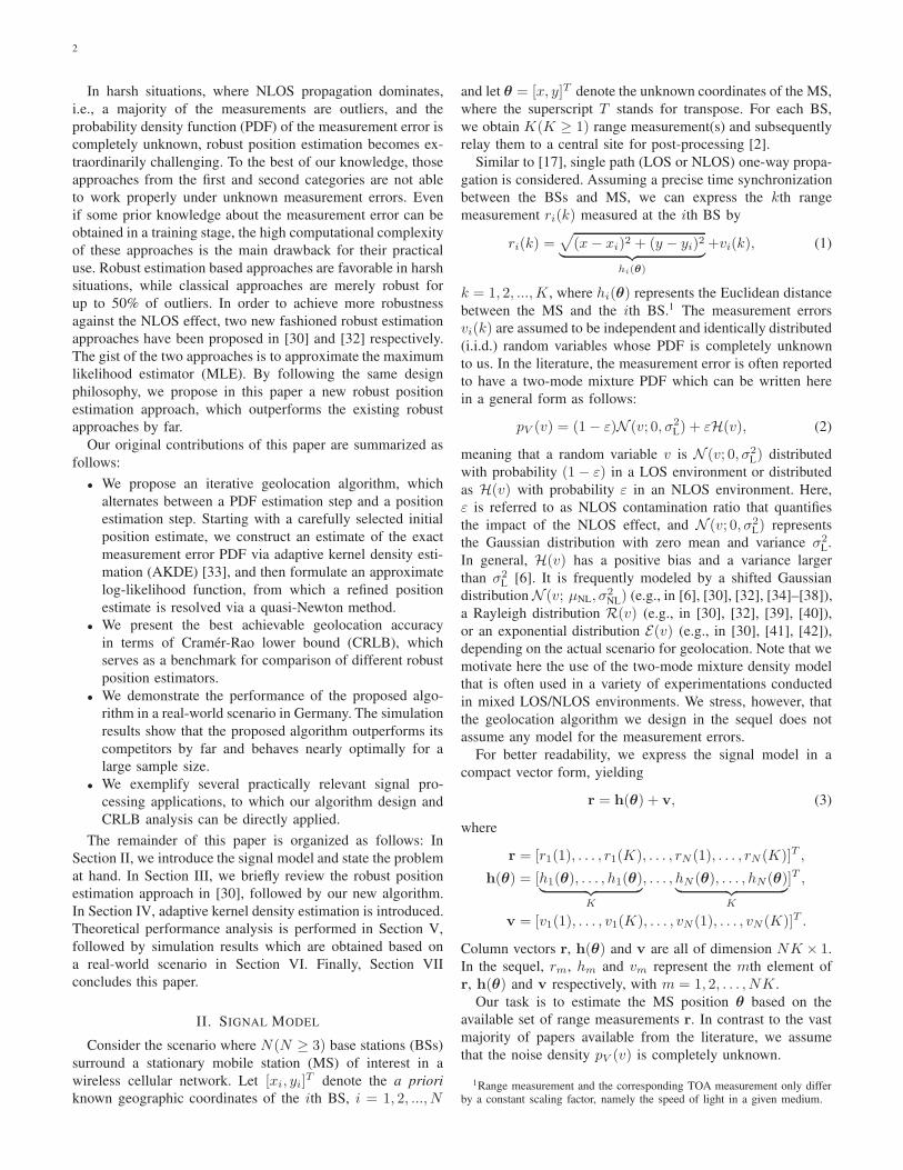
VI. SIMULATIONS

We consider geolocation of a stationary MS in a cellular

radio network which comprises N BSs with fixed and known

geographic coordinates. In order to be as realistic as possible,

the BS locations are taken from an operating cellular radio

network in a German city center [36], [60]. The geometry

of the BSs as well as the approximate location of the city

center is shown in Fig. 1. The BS antennae are generally

deployed on rooftops, and the city center can be characterized

as urban with multi-storey buildings and narrow streets. Field

trials conducted in this city have revealed that the TOA

measurement error can be well approximated by a Gaussian

mixture distribution [36]. In the simulations, we generate range

measurement errors from the following two-mode Gaussian

mixture distribution

pV (v) = (1− ε)N (v; 0, σ2L) + εN (v;µNL, σ

2NL) (37)

as mentioned in Section II. The parameters of the Gaussian

mixture as well as all other simulation parameters are sum-

marized in Table I.

The newly proposed robust iterative nonparametric estima-

tor is compared to the following position estimators:

• Least-squares estimator, cf. (16)

• Robust M-estimator [29], [30]

• Robust semi-parametric estimator [30]

• Robust nonparametric estimator [32]

• MLE with known pV (v)

The first three approaches are all developed under the linear

regression model in (10). In the robust M-estimation approach,

the clipping point c of Huber’s score function ψ(v; c) (cf. [30,

(7)]) is adaptively calculated by c = 0.6/(1.483 · mad(ˆv)),where ˆv denotes the a priori extracted residual vector in each

iteration and mad(·) denotes the median absolute deviation. In

the semi-parametric approach [30], we choose the same trans-

formation function t(ˆv; ζ) and search interval [ζL = 0.9, ζU =1] as suggested therein. The robust nonparametric approach

follows Algorithm 1, except that the number of iterations is

constrained to one. By assuming pV (v) to be known, we

resolve the MLE, serving as a benchmark for comparison,

from (4) via the quasi-Newton method (cf. Algorithm 2) with

−2000 −1500 −1000 −500 0 500 1000 1500 2000−1500

−1000

−500

0

500

1000

1500

city−center

BSs

x-position (meter)

y-p

osi

tion

(met

er)

Fig. 1. 2-D illustration of the geometry of BSs and the city center area ina real-world scenario in Germany.

0.2

5879

0.25879

0.25879

0.25879

0.2

5933

0.25

933

0.25933

0.25933

0.25933

0.2

5987

0.25987 0.25987

0.25987

0.25987

0.26041 0.26041

0.26041

0.26041

0.260960.26096

0.26096

0.26096

0.26150.2615

0.2615

0.2615

0.262040.26204 0.26204

0.26204

0.262580.26258 0.26258

0.2

6258

0.26312

0.26312

0.26312

0.2

6312

0.26366

0.263660.26366

0.2

6366

0.26420.2642

0.2

642

0.264750.26475

0.265290.265290.26583

0.26637

−500 −400 −300 −200 −100 0 100 200 300 400 500−500

−400

−300

−200

−100

0

100

200

300

400

500

x-position (meter)

y-p

osi

tion

(met

er)

Fig. 2. GDOP values measured for an efficient position estimator in the citycenter area with K = 1 and ε = 0.5.

the initial guess set by the true MS position. Apart from the

MLE, the rest of estimators do not assume pV (v) to be known

a priori.

A. Geometric Dilution of Precision

In the first simulation, GDOP values are computed accord-

ing to (36) (i.e., assuming an efficient position estimator)

for various different positions in the city center area as

illustrated in Fig. 1. In this simulation, the number of range

measurements K obtained at each BS is set to one and the

NLOS contamination ratio ε is set to 0.5. By following the

results derived in [50, Section 1.4.16], σv in (36) is calculated

by

σv =√

(1− ε) · σ2L + ε · σ2

NL + ε · (1− ε) · µ2NL. (38)

The resulting GDOP values are shown in Fig. 2, and they

indicate a well-suited geometry of the BSs for locating a MS in

8

0 0.1 0.2 0.3 0.4 0.5 0.6 0.7 0.8 0.9 1−5

0

5

10

15

20

25

30

35

40

45

50

LS−Est

Robust−M−Est

Robust SemiPara−Est

Robust−NonPara−Est

Proposed

MLE

Contamination ratio, ε

Bia

s(x)

(met

er)

(a)

0 0.1 0.2 0.3 0.4 0.5 0.6 0.7 0.8 0.9 1−5

0

5

10

15

20

25

30

35

40

45

50

LS−Est

Robust−M−Est

Robust−SemiPara−Est

Robust−NonPara−Est

Proposed

MLE

Contamination ratio, ε

Bia

s(y)

(met

er)

(b)

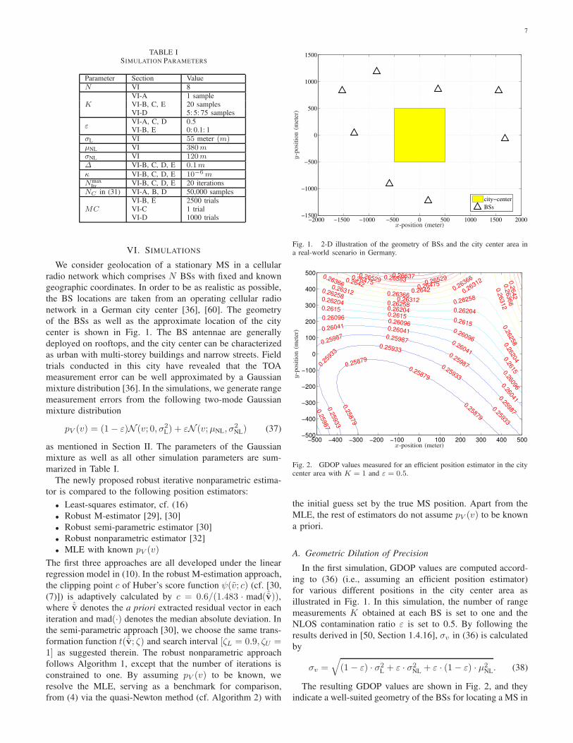
Fig. 3. Bias (assuming a fixed set of geographic coordinates [x =0.25 km, y = 0.25 km]T ) of the different position estimators versus NLOScontamination ratio ε with K = 20. (a) describes the bias in x-position; and(b) describes the bias in y-position.

the city center area. When we further increase K or decrease

ε, better GDOP values are achievable. A proper discussion on

the impact of BSs-MS geometry on the geolocation accuracy

is out of the scope of our paper. Interested readers are referred

to [8, Chapter 13] and references therein.

B. Bias, RMSE and CRLB

In this simulation, the different position estimators are

evaluated in terms of bias and RMSE. To this end, the bias and

the RMSE of the different position estimators are evaluated in

a large-scale Monte Carlo simulation with MC = 2500 trials.

Two examples are investigated in the sequel.

The first example assumes that the MS is located at [x =250m, y = 250m]T and the number of range measurements

at each BS is K = 20 samples. The bias and RMSE of the

0 0.1 0.2 0.3 0.4 0.5 0.6 0.7 0.8 0.9 10

20

40

60

80

100

120

LS−Est

Robust−M−Est

Robust−SemiPara−Est

Robust−NonPara−Est

Proposed

MLECRLB

Pos

Contamination ratio, ε

RM

SE

(met

er)

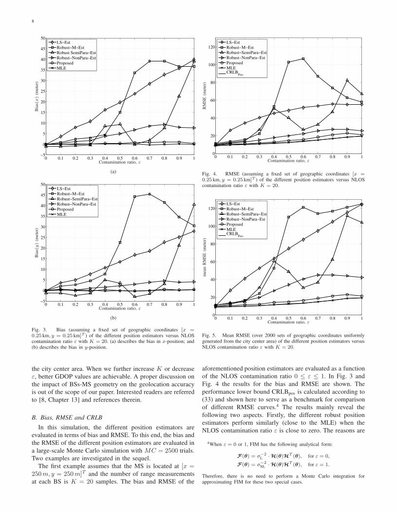
Fig. 4. RMSE (assuming a fixed set of geographic coordinates [x =0.25 km, y = 0.25 km]T ) of the different position estimators versus NLOScontamination ratio ε with K = 20.

0 0.1 0.2 0.3 0.4 0.5 0.6 0.7 0.8 0.9 10

20

40

60

80

100

120

LS−Est

Robust−M−Est

Robust−SemiPara−Est

Robust−NonPara−Est

Proposed

MLECRLB

Pos

Contamination ratio, ε

mea

nR

MS

E(m

eter

)

Fig. 5. Mean RMSE (over 2000 sets of geographic coordinates uniformlygenerated from the city center area) of the different position estimators versusNLOS contamination ratio ε with K = 20.

aforementioned position estimators are evaluated as a function

of the NLOS contamination ratio 0 ≤ ε ≤ 1. In Fig. 3 and

Fig. 4 the results for the bias and RMSE are shown. The

performance lower bound CRLBpos is calculated according to

(33) and shown here to serve as a benchmark for comparison

of different RMSE curves.4 The results mainly reveal the

following two aspects. Firstly, the different robust position

estimators perform similarly (close to the MLE) when the

NLOS contamination ratio ε is close to zero. The reasons are

4When ε = 0 or 1, FIM has the following analytical form:

F(θ) = σ−2

L ·H(θ)HT (θ), for ε = 0,

F(θ) = σ−2

NL ·H(θ)HT (θ), for ε = 1.

Therefore, there is no need to perform a Monte Carlo integration forapproximating FIM for these two special cases.

9

−400 −200 0 200 400 600 800 1000 12000

0.5

1

1.5

2

2.5

3

3.5

4x 10

−3

Estimated PDF on the First Itr

Estimated PDF on the Last Itr

True PDF

v (meter)

PD

F

Fig. 6. A comparison among the exact measurement error PDF pV (v) (blacksolid line), the PDF estimated on the last iteration of Algorithm 1 (red dashedline) and the PDF estimated on the first iteration of the Algorithm 1 (as sameas the one constructed in the robust nonparametric approach [32]) (blue dash-dot line) in a particular Monte Carlo trial with [x = 250m, y = 250m]T ,K = 20 samples and ε = 0.5.

as follows:

1) For the first two robust estimators developed under the

linear regression model, the measurement error vi(k) is

most probably generated from the LOS mixture com-

ponent N (v; 0, σ2L) resulting in vi(k) ≈ 2hi(θ) · vi(k)

in (8) for our simulation scenario. As a result, vi(k),i = 1, 2, ..., N and k = 1, 2, ...,K can be regarded as

approximately jointly Gaussian distributed, and it was

shown in [29], [30] that they perform nearly optimally

under the Gaussian model.

2) Due to the good quality of the initial guess (i.e., the

least-squares estimate), the estimated measurement error

PDF obtained on the first iteration of Algorithm 1 is

already close to the exact PDF and extra iterations can

only ameliorate it slightly. This explains why the robust

nonparametric estimator and the new proposed one show

similar performance as that of the MLE.

Secondly, the new proposed estimator is closest to the MLE

and outperforms by far all the other robust competitors when

ε is large. The reasons are as follows:

1) When ε is large, the PDF of vi(k) starts to deviate from

the Gaussian model, leading to deteriorated performance

of the robust estimators developed under the linear

regression model.

2) The robust M-estimator breaks down at best for a

contamination ratio equal to 0.5 [14]. Therefore, it is

not surprising to see the drastic performance degradation

from ε > 0.3 in Fig. 4.

3) The existing robust semi-parametric estimator [30] per-

forms even worse than the least-squares estimator or

the robust M-estimator for some ε (e.g., ε = 0.9in Fig. 4). The reason may lie in the fact that the

transformation function t(ˆv; ζ) and the associated search

−400 −200 0 200 400 600 800 1000 12000

5

10

15

Exact Measurement Errors

−400 −200 0 200 400 600 800 1000 12000

5

10

15

Final Residuals

v (meter)

Fre

qC

ounts

Fre

qC

ounts

Fig. 7. Histogram of the exact measurement errors (upper) versus thehistogram of the residuals extracted on the last iteration of Algorithm 1 (lower)in the same Monte Carlo trial. Note that the sum of frequency counts shownin this figure is equal to the number of measurements, NK = 160 samples.

interval [ζL = 0.9, ζU = 1] needed in the TKDE are

inappropriate for our assumed simulation scenario. 5

4) Having conquered the drawbacks of the existing semi-

parametric approach (cf. Section III-A), we harvest

improved performance in terms of bias and RMSE in

both the robust nonparametric approach [32] and the

newly proposed approach.

5) Since the quality of the initial guess (i.e., the least-

squares estimate) degenerates as ε increases, larger

discrepancy has been observed between the exact mea-

surement error PDF pV (v) and its estimate calculated

on the first iteration of Algorithm 1. Therefore, the

robust nonparametric approach becomes worse as εincreases. Introducing extra iterations in the newly pro-

posed approach, we successfully reduce the discrepancy

and consequently achieve further improved geolocation

accuracy.

In the second example, the overall performance of the

position estimators in the city center area is examined. We

generate 2000 sets of different geographic coordinates [x, y]T

uniformly from the city center area, calculate the RMSE

and CRLBpos for each set, and finally average them all. The

results are shown in Fig. 5, from which we observe that the

performance of the proposed estimator and MLE stays almost

unaltered while the performance of the others becomes worse.

Here, it is noteworthy that the RMSE curve of the MLE

coincides well with the corresponding CRLBpos curve in Fig. 4

and Fig. 5.

C. Measurement Error PDF Estimation via AKDE

In the previous simulation, we have seen a performance

improvement in the newly proposed approach as compared to

5The transformation function t(v; ζ) and the associated search interval forζ , [ζL = 0.9, ζU = 1], were demonstrated to be optimal for the simulationscenario defined in [30] which is different from ours.

10

the robust nonparametric approach. As analyzed beforehand,

this improvement mainly stems from the extra enhancement

in the PDF estimation achieved in the new algorithm. In order

to confirm our statement, Fig. 6 shows the PDF estimates

obtained on different iterations of Algorithm 1 versus the exact

measurement error PDF for a particular Monte Carlo trial in

the first example of Section VI-B. Moreover, Fig. 7 shows

the histogram of both the exact measurement errors and final

residuals (cf. Step 2 of Algorithm 1) of this particular trial.

It is worth emphasizing that the enhancement in the PDF

estimation is clearly seen in almost every trial, but due to

space limitations only one snapshot is shown here.

D. Estimation Efficiency

Next, we show the estimation efficiency of the proposed

position estimator as a function of the number of measure-

ments. Here, we assume that the MS is located at [x =250m, y = 250m]T , K varies from 5 to 75 at an increment

of 5 samples and ε = 0.5. For each K , MC = 1000 Monte

Carlo trials are carried out to calculate the RMSE, and then

the estimation efficiency according to (34) is evaluated. Fig. 8

shows the resulting estimation efficiency versus the number

of measurements at each BS. Gathering these results, we

summarize the performance of the newly proposed estimator

as follows:

- It performs closer to the MLE as NK increases. The

estimation efficiency of the MLE is very close to one

when NK ≥ 450 samples.

- It achieves good estimation efficiency for large NK .

When NK = 100 samples are available, it attains an

efficiency of η ≈ 0.8; When we further increase NKto 300 samples, the efficiency is η ≈ 0.9; Although

not shown here, the efficiency will increase very slowly

thereafter and attain η ≈ 1 at NK = 1000 samples.

- It largely deviates from the MLE when NK is small (e.g.,

NK ≤ 50 samples), but still outperforms other robust

estimators by far.

In addition, we also found that the existing robust semi-

parametric estimator in [30] does not fulfill the asymptotic

efficiency property.

E. Computational Complexity and Speed of Convergence

One of the most important location-based services is the

E-911 service, where the time consumed in estimating the po-

sition of a caller in emergency must be restricted to 30 seconds

[8]. In order to examine our new approach in this aspect, we

calculate the average computational time it requires to give

an individual position estimate in the second simulation. The

results in Table II show that the average computational time

of the new approach is higher than other approaches, but it is

still acceptable for the emergency use. Besides, it needs circa

6 iterations on average for Algorithm 1 to converge. 6

6All the simulations have been performed under MATLABTMR2010a en-vironment on a PC equipped with Intel R©CoreTM i5-760 processor (2.80GHz)and 8GB RAM.

10 20 30 40 50 60 700.2

0.3

0.4

0.5

0.6

0.7

0.8

0.9

1

1.1

Robust−SemiPara−Est

Robust−NonPara−Est

Proposed

MLE

Ideal Efficient−Est

K (samples)

Effi

cien

cy,η

Fig. 8. Estimation efficiency η of different position estimators versus thenumber of measurements collected at each of N = 8 BSs, K .

TABLE IIAVERAGE COMPUTATIONAL TIME FOR GENERATING A SINGLE POSITION

ESTIMATE IN THE SECOND SIMULATION

Name Computational time

Least-squares approach < 0.0001 sec.Robust M-estimation approach 0.0789 sec.Robust semi-parametric approach 0.6273 sec.Robust nonparametric approach 0.6580 sec.Proposed approach 2.4284 sec.E-911 requirement < 30 sec.

F. Remark on Simulation Results and Practical Implementa-

tion

In the above simulations, we focus on the Gaussian mixture

model, although the proposed algorithm is able to work for

any other model. The overwhelming reason is that a Gaussian

mixture can approximate any other distribution arbitrarily well

in, for instance, the L1 norm. Therefore, we find the Gaussian

mixture case is the most representative example. For rigor, we

have also tested the newly proposed approach in the scenarios

where different measurement error distributions (e.g., the two-

mode Gaussian-Rayleigh and Gaussian-exponential mixture)

and simulated BS geometries (e.g., the one utilized in [32]).

Similar conclusions can be drawn in these cases.

Here, we use N = 8 BSs for geolocation. However, in

practice, not all of the possible BSs are detectable, implying

a smaller N is available. In this case, our algorithm will

show moderately degraded performance in the localization (cf.

Section VI-B) and PDF approximation (cf. Section VI-C) in

the above examples, since less total number of measurements

NK are available. However, the key conclusions drawn in

Section VI would not change at all. In order to compensate

for the performance loss due to the smaller N , we can simply

collect more samples, K , at each BS.

Moreover, we briefly discuss two important aspects con-

cerning practical implementation of our proposed algorithm.

The first one is how to predetermine K—the number of

measurements collected at each BS. It can be determined in

11

an offline training phase as follows: First, we test different

Ks for each of the positions in an area of interest and register

the resulting geolocation accuracies produced by our proposed

algorithm. Next, we choose the smallest K amongst all tested

values that satisfies the given requirement(s), e.g., the Fed-

eral Communications Commission (FCC) requirement, for the

subsequent online localization phase. The second aspect lies in

the selection of an initial position estimate. Our preference is

the least-squares position estimate. If it is found unreliable, we

could resort to the sophisticated strategy presented previously.

Besides, we could also integrate the information, if available,

from global positioning system (GPS) or assisted-GPS.

G. Remark on Possible Applications

Before concluding our paper, another important remark is

given here. In fact, the route we have followed to design the

new robust position estimator in Section III and compute the

Cramer-Rao lower bound in Section V are directly applicable

to a general measurement model, where r is a measurement

vector, θ is a deterministic vector parameter to be determined,

h(θ) is an arbitrary nonlinear mapping matrix, and v is a non-

Gaussian noise vector of i.i.d. elements with unknown PDF.

Many signal processing problems arrive at this generalized

measurement model, for instance:

1) Geolocation using a single moving receiver with any

type of measurements such as TOA, TDOA, RSS and

AOA, e.g., [8, Chap. 17].

2) Source localization and tracking in wireless sensor net-

works, e.g., [61].

3) Direction-of-arrival (DOA) estimation in non-Gaussian

noise, e.g., [62].

4) Amplitude estimation of sinusoidal signals in non-

Gaussian noise, e.g., [63].

VII. CONCLUSION

We have developed an iterative algorithm for robust posi-

tion estimation in harsh line-of-sight/non-line-of-sight environ-

ments, where the measurement error is assumed to be com-

pletely unknown. We have also presented the best achievable

geolocation accuracy in terms of the CRLB in the assumed

situation. Simulations have been performed both in the real-

world and simulated scenarios. The results show that the

proposed position estimator achieves significantly improved

performance. Especially when the number of range measure-

ments is large, our new proposed position estimator is very

close to the MLE and the geolocation accuracy approaches

the best achievable performance. However, the improvement

comes at the expense of higher computation as compared to

other competitors.

APPENDIX A

PROOF OF THE DIAGONAL PROPERTY OF Iv

Due to the statistical properties of the vector elements vm,

m = 1, 2, ..., NK , the (m,m′)th entry of the matrix Iv can

be expressed by

[Iv]m,m′ = Epv(v)

{∇vmpV (vm) · ∇vm′pV (vm′)

pV (vm) · pV (vm′)

}

. (39)

If m = m′, the mth main diagonal element is simplified to

[Iv]m,m = Ivm = EpV (vm)

{

[∇vmpV (vm)]2

[pV (vm)]2

}

. (40)

Since vm, m = 1, 2, ..., NK are identically distributed, we

can conclude that

Iv = Iv1 = Iv2 = ... = IvNK. (41)

if m 6= m′, [Iv]m,m′ is equal to

EpV (vm)

{∇vmpV (vm)

pV (vm)

}

·EpV (vm′ )

{∇vm′pV (vm′)

pV (vm′)

}

, (42)

since vm and vm′ are mutually independent. In order to prove

the diagonal property of Iv, we recall that for the computation

of the CRLB, the following regularity condition

Ep(r|θ) {∇θ log p(r | θ)} = 0 (43)

must hold for any θ. Performing the chain rule [55] upon

∇θ log p(r | θ) in (43), we can easily obtain

[∇θh(θ)] · Epv(v)

{∇vpv(v)

pv(v)

}

= 0 (44)

for any θ, implying that

EpV (v)

{∇vpV (v)

pV (v)

}

= 0, (45)

because the elements in v are i.i.d.. As a result, [Iv]m,m′ = 0for m 6= m′ and [Iv]m,m′ = Iv for m = m′, i.e., Iv =Iv · INK is proven.

REFERENCES

[1] A. H. Sayed, A. Tarighat, and N. Khajehnouri, “Network-based wirelesslocation: challenges faced in developing techniques for accurate wirelesslocation information,” IEEE Signal Process. Mag., vol. 22, no. 4, pp.24–40, Jul. 2005.

[2] J. J. Caffery and G. L. Stuber, “Overview of radiolocation in CDMAcellular systems,” IEEE Commun. Mag., vol. 36, no. 4, pp. 38–45, Apr.1998.

[3] A. Amar and A. J. Weiss, “Localization of narrowband radio emittersbased on Doppler frequency shifts,” IEEE Trans. Signal Process.,vol. 56, no. 11, pp. 5500–5508, Nov. 2008.

[4] A. J. Weiss, “Direct geolocation of wideband emitters based on delayand Doppler,” IEEE Trans. Signal Process., vol. 59, no. 6, pp. 2513–2521, Jun. 2011.

[5] J. J. Caffery, Wireless Location in CDMA Cellular Radio System.Norwell, MA: Kluwer Academic Publisher, 1999.

[6] F. Gustafsson and F. Gunnarsson, “Mobile positioning using wirelessnetworks: possibilities and fundamental limitations based on availablewireless network measurements,” IEEE Signal Process. Mag., vol. 22,no. 4, pp. 41–53, Jul. 2005.

[7] S. Gezici, “A survey on wireless position estimation,” Wireless Pers.

Commun., vol. 44, pp. 263–282, Feb. 2008.[8] R. Zekavat and R. M. Buehrer, Handbook of Position Location. Hobo-

ken, NJ: John Wiley & Sons, Inc., 2011.[9] Y. T. Chan and K. C. Ho, “A simple and efficient estimator for hyperbolic

location,” IEEE Trans. Signal Process., vol. 42, no. 8, pp. 1905–1915,Aug. 1994.

[10] K. W. Cheung, H. C. So, W. K. Ma, and Y. T. Chan, “Least squares al-gorithms for time-of-arrival-based mobile location,” IEEE Trans. Signal

Process., vol. 52, no. 4, pp. 1121–1130, Apr. 2004.[11] K. W. Cheung and H. C. So, “A multidimensional scaling framework

for mobile location using time-of-arrival measurements,” IEEE Trans.

Signal Process., vol. 53, no. 2, pp. 460–470, Feb. 2005.[12] H.-W. Wei, Q. Wan, Z.-X. Chen, and S.-F. Ye, “A novel weighted multi-

dimensional scaling analysis for time-of-arrival-based mobile location,”IEEE Trans. Signal Process., vol. 56, no. 7, pp. 3018–3022, Jul. 2008.

12

[13] H. C. So and F. K. W. Chan, “A generalized subspace approach formobile positioning with time-of-arrival measurements,” IEEE Trans.

Signal Process., vol. 55, no. 10, pp. 5103–5107, Oct. 2007.

[14] H. C. So, Y. T. Chan, and F. K. W. Chan, “Closed-form formulaefor time-difference-of-arrival estimation,” IEEE Trans. Signal Process.,vol. 56, no. 6, pp. 2614–2620, Jun. 2008.

[15] Y. T. Chan, W. Y. Tsui, H. C. So, and P. C. Ching, “Time-of-arrivalbased localization under NLOS conditions,” IEEE Trans. Veh. Technol.,vol. 55, no. 1, pp. 17–24, Jan. 2006.

[16] J. Riba and A. Urruela, “A non-line-of-sight mitigation technique basedon ML-detection,” in Proc. IEEE Int. Conf. Acoustics, Speech, and

Signal Processing (ICASSP), vol. 2, Montreal, Quebec, Canada, May2004, pp. 153–156.

[17] Y. H. Qi, H. Kobayashi, and H. Suda, “Analysis of wireless geolocationin a non-line-of-sight environment,” IEEE Trans. Wireless Commun.,vol. 5, no. 3, pp. 672–681, Mar. 2006.

[18] X. Wang, Z. X. Wang, and B. O’Dea, “A TOA-based location algorithmreducing the errors due to non-line-of-sight (NLOS) propagation,” IEEE

Trans. Veh. Technol., vol. 52, no. 1, pp. 112–116, Jan. 2003.

[19] S. Venkatesh and R. M. Buehrer, “A linear programming approach toNLOS error mitigation in sensor networks,” in Proc. IEEE Int. Conf.Information Processing in Sensor Networks (IPSN), Nashville, TN,USA, Apr. 2006, pp. 301–308.

[20] H. Y. Chen, G. Wang, Z. Z. Wang, H. C. So, and H. V. Poor, “Non-line-of-sight node localization based on semi-definite programming inwireless sensor networks,” IEEE Trans. Wireless Commun., vol. 11,no. 1, pp. 108–116, Jan. 2012.

[21] R. A. Maronna, R. D. Martin, and V. J. Yohai, Robust Statistics: Theoryand Methods. Chichester, England: John Wiley & Sons Ltd., 2006.

[22] P. J. Huber and E. M. Ronchetti, Robust Statistics. Hoboken, NJ: JohnWiley & Sons Ltd., 2009.

[23] Z. Li, W. Trappe, Y. Zhang, and B. Nath, “Robust statistical methods forsecuring wireless localization in sensor networks,” in Proc. IEEE Int.Symp. Information Processing in Sensor Networks (IPSN), Los Angeles,CA, Apr. 2005, pp. 91–98.

[24] R. Casas, A. Marco, J. J. Guerrero, and J. Falco, “Robust estimator fornon-line-of-sight error mitigation in indoor localization,” EURASIP J.Appl. Signal Process., vol. 2006, no. 1, pp. 1–8, Jan. 2006.

[25] G. L. Sun and W. Guo, “Bootstrapping M-estimators for reducing errorsdue to non-line-of-sight (NLOS) propagation,” IEEE Commun. Lett.,vol. 8, no. 8, pp. 509–510, Aug. 2004.

[26] A. M. Zoubir and D. R. Iskander, Bootstrap Techniques for Signal

Processing. Cambridge, U.K.: Cambridge University Press, 2004.

[27] A. M. Zoubir and B. Boashash, “The bootstrap and its application insignal processing,” IEEE Signal Process. Mag., vol. 15, no. 1, pp. 56–76,Jan. 1998.

[28] A. M. Zoubir and D. R. Iskander, “Bootstrap methods and applications,”IEEE Signal Process. Mag., vol. 24, no. 4, pp. 10–19, Jul. 2007.

[29] U. Hammes, “Robust positioning algorithm for wireless networks,”Ph.D. dissertation, Technische Universitat Darmstadt, Dec. 2009.

[30] U. Hammes, E. Wolsztynski, and A. M. Zoubir, “Robust tracking andgeolocation for wireless networks in NLOS environments,” IEEE J. Sel.

Topics. Signal Process., vol. 3, no. 5, pp. 889–901, Oct. 2009.

[31] I. Guvenc and C. C. Chong, “A survey on TOA based wireless localiza-tion and NLOS mitigation techniques,” Commun. Surveys Tuts., vol. 11,no. 3, pp. 107–124, third quarter 2009.

[32] F. Yin and A. M. Zoubir, “Robust positioning in NLOS environmentsusing nonparametric adaptive kernel density estimation,” in Proc. IEEEInt. Conf. Acoustics, Speech and Signal Processing (ICASSP), Kyoto,Japan, Mar. 2012, pp. 3517–3520.

[33] B. W. Silverman, Density Estimation: for Statistical and Data Analysis.London: Chapman and Hall, 1986.

[34] J.-F. Liao and B.-S. Chen, “Robust mobile location estimator with NLOSmitigation using interacting multiple model algorithm,” IEEE Trans.

Wireless Commun., vol. 5, no. 11, pp. 3002–3006, Nov. 2006.

[35] C. Fritsche, U. Hammes, A. Klein, and A. M. Zoubir, “Robust mobileterminal tracking in NLOS environments using interacting multiplemodel algorithm,” in Proc. IEEE Int. Conf. Acoustics, Speech and Signal

Processing (ICASSP), Taipei, Taiwan, Apr. 2009, pp. 3049–3052.

[36] C. Fritsche and A. Klein, “On the performance of mobile terminal track-ing in urban GSM networks using particle filters,” in Proc. European

Signal Process. Conf. (EUSIPCO), Glasgow, Scotland, Aug. 2009, pp.1953–1957.

[37] U. Hammes and A. M. Zoubir, “Robust mobile terminal tracking inNLOS environments based on data association,” IEEE Trans. Signal

Process., vol. 58, no. 11, pp. 5872–5882, Nov. 2010.

[38] ——, “Robust MT tracking based on M-estimation and interactingmultiple model algorithm,” IEEE Trans. Signal Process., vol. 59, no. 7,pp. 3398–3409, Jul. 2011.

[39] J. M. Huerta and J. Vidal, “Mobile tracking using UKF, time measuresand LOS-NLOS expert knowledge,” in Proc. IEEE. Int. Conf. Acoustics,

Speech, and Signal Processing (ICASSP), vol. 4, Philadelphia, PA, USA,Mar. 2005, pp. 901–904.

[40] L. Cong and W. Zhuang, “Nonline-of-sight error mitigation in mobilelocation,” IEEE Trans. Wireless Commun., vol. 4, no. 2, pp. 560–573,Mar. 2005.

[41] P. C. Chen, “A non-line-of-sight error mitigation algorithm in locationestimation,” in Proc. IEEE Int. Conf. Wireless Commun. Networking

(WCNC), vol. 1, New Orleans, LA, Sep. 1999, pp. 316–320.[42] M. McGuire, K. N. Plataniotis, and A. N. Venetsanopoulos, “Data fusion

of power and time measurements for mobile terminal location,” IEEETrans. Mobile Comput., vol. 4, no. 2, pp. 142–153, Mar./Apr. 2005.

[43] U. Hammes, E. Wolsztynski, and A. M. Zoubir, “Transformation-basedrobust semiparametric estimation,” IEEE Signal Process. Letters, vol. 15,pp. 845–848, 2008.

[44] A. M. Zoubir and R. F. Brcich, “Multiuser detection in heavy tailednoise,” Digital Signal Process., vol. 12, no. 2-3, pp. 262–273, 2002.

[45] A. Beck, P. Stoica, and J. Li, “Exact and approximate solutions of sourcelocalization problems,” IEEE Trans. Signal Process., vol. 56, no. 5, pp.1770–1778, May 2008.

[46] C. T. Kelley, Solving nonlinear equations with Newton’s method, ser.Fundamentals of Algorithms. Philadelphia, PA: Society for Industrialand Applied Mathematics (SIAM), 2003.

[47] R. Fletcher, Practical methods of optimization (2nd ed.). Chichester,England: John Wiley & Sons Ltd., 1987.

[48] J. A. Bilmes, “A gentle tutorial on the EM algorithm and its applicationto parameter estimation for Gaussian mixture and hidden Markovmodels,” University of California, Berkeley, Berkeley, CA, USA, Tech.Rep., 1998.

[49] S. Kay, Fundamentals of Statistical Signal Processing: Estimation

Theory. Englewood Cliffs, NJ: Prentice-Hall, Inc., 1993.[50] Y. Bar-Shalom, X. R. Li, and T. Kirubarajan, Estimation with Applica-

tions to Tracking and Navigation. New York, NY: John Wiley & Sons,Inc., 2001.

[51] J. Nocedal and S. J. Wright, Numerical optimization. New York, NY:Springer-Verlag New York, Inc., 1999.

[52] I. S. Abramson, “On bandwidth variation in kernel estimates—a squareroot law,” Ann. Statist., vol. 10, no. 4, pp. 1217–1223, 1982.

[53] F. Gustafsson, Statistical Sensor Fusion. Lund, Sweden: Studentlitter-atur, 2012.

[54] C. P. Robert and G. Casella, Monte Carlo Statistical Methods. NewYork, NY: Springer-Verlag, 1999.

[55] E. L. Lehmann and G. Casella, Theory of point estimation. New York,NY: Springer-Verlag, Inc., 1998.

[56] H. L. Van Trees, Optimum Array Processing. Part IV of Detection,

Estimation, and Modulation Theory. John Wiley & Sons, Inc., NewYork, USA, 2002.

[57] G. Hendeby, “Performance and implementation aspects of nonlinearfiltering,” Ph.D. dissertation, Linkoping University, Linkoping, Sweden,Feb. 2008.

[58] K. C. Ho, “Bias reduction for an explicit solution of source localizationusing TDOA,” IEEE Trans. Signal Process., vol. 60, no. 5, pp. 2101–2114, May 2012.

[59] N. Levanon, “Lowest GDOP in 2-D scenarios,” Proc. IEE Radar, Sonar

and Navigation, vol. 147, no. 3, pp. 149–155, Jun. 2000.[60] C. Fritsche, “Statistical data fusion for hybrid localization of mobile

terminals,” Ph.D. dissertation, Technische Universitat Darmstadt, Mar.2011.

[61] Y. Liu, Y.-H. Hu, and Q. Pan, “Distributed, robust acoustic sourcelocalization in a wireless sensor network,” IEEE Trans. Signal Process.,vol. 60, no. 8, pp. 4350–4359, Aug. 2012.

[62] R. J. Kozick and B. M. Sadler, “Maximum-likelihood array processingin non-Gaussian noise with Gaussian mixtures,” IEEE Trans. Signal

Process., vol. 48, no. 12, pp. 3520–3535, Dec. 2000.[63] P. Stoica, H.-B. Li, and J. Li, “Amplitude estimation of sinusoidal

signals: survey, new results, and an application,” IEEE Trans. Signal

Process., vol. 48, no. 2, pp. 338–352, Feb. 2000.

13

Feng Yin received the B.Sc. degree from Shang-hai Jiao Tong University, China in 2008, and theM.Sc. degree from Technische Universitat Darmstadt(TUD), Darmstadt, Germany in 2011.

He is currently working towards the Ph.D. degreein the Signal Processing Group (SPG) at TechnischeUniversitat Darmstadt. His research interests includeoptimal waveform design, robust estimation theorywith applications to wireless geolocation, trackingand navigation.

Carsten Fritsche received the Dipl.-Ing. degreein 2005 and the Dr.-Ing. degree in 2011 both inelectrical engineering and information technologyfrom Technische Universitat Darmstadt, Germany. In2011 he joined the Division of Automatic Controlat Linkoping University, Sweden, as a postdoctoralresearch fellow. Since spring 2012, he has beenwith IFEN GmbH, Poing, Germany, working asa systems engineer on satellite navigation relatedprojects. His main research interest lies in the areaof statistical signal processing, machine learning and

sensor fusion with applications to wireless positioning and satellite navigation.

Fredrik Gustafsson is professor in Sensor In-formatics at Department of Electrical Engineering,Linkoping University, since 2005. He received theM.Sc. degree in electrical engineering 1988 and thePh.D. degree in Automatic Control, 1992, both fromLinkoping University. During 1992-1999 he heldvarious positions in automatic control, and 1999-2005 he had a professorship in Communication Sys-tems. His research interests are in stochastic signalprocessing, adaptive filtering and change detection,with applications to communication, vehicular, air-

borne, and audio systems. He is a co-founder of the companies NIRADynamics (automotive safety systems), Softube (audio effects) and SenionLab(indoor positioning systems).

He was an associate editor for IEEE Transactions on Signal Process-ing 2000-2006 and is currently associate editor for IEEE Transactions onAerospace and Electronic Systems and EURASIP Journal on Applied SignalProcessing. He was awarded the Arnberg prize by the Royal SwedishAcademy of Science (KVA) 2004, elected member of the Royal Academy ofEngineering Sciences (IVA) 2007, elevated to IEEE Fellow 2011 and awardedthe Harry Rowe Mimno Award 2011 for the tutorial ”Particle Filter Theoryand Practice with Positioning Applications”, which was published in the AESSMagazine in July 2010.

Abdelhak M. Zoubir is a Fellow of the IEEEand IEEE Distinguished Lecturer (Class 2010-2011).He received his Dr.-Ing. from Ruhr- UniversitatBochum, Germany in 1992. He was with QueenslandUniversity of Technology, Australia from 1992-1998where he was Associate Professor. In 1999, hejoined Curtin University of Technology, Australia asa Professor of Telecommunications and was InterimHead of the School of Electrical & Computer Engi-neering from 2001 until 2003. In 2003, he movedto Technische Universitat Darmstadt, Germany as

Professor of Signal Processing and Head of the Signal Processing Group. Hisresearch interest lies in statistical methods for signal processing with emphasison bootstrap techniques, robust detection and estimation and array processingapplied to telecommunications, radar, sonar, automotive monitoring and safety,and biomedicine. He published over 300 journal and conference papers onthese areas. Professor Zoubir was the Technical Chair of the 11th IEEEWorkshop on Statistical Signal Processing (SSP 2001), General Co-Chair ofthe 3rd IEEE International Symposium on Signal Processing & InformationTechnology (ISSPIT 2003) and of the 5th IEEE Workshop on Sensor Arrayand Multi-channel Signal Processing (SAM 2008). He is the General Co-Chair of the 14th International Workshop on Signal Processing Advances inWireless Communications (SPAWC 2013) to be held in Darmstadt, Germany,the General Co-Chair of the 21st European Signal Processing Conference(EUSIPCO 2013) to be held in Marrakech, Morocco, and the Technical Co-Chair of ICASSP-14 to be held in Florence, Italy. Dr. Zoubir was an AssociateEditor of the IEEE Transactions on Signal Processing (1999-2005), a Memberof the Senior Editorial Board of the IEEE Journal on Selected Topics in SignalProcessing (2009-2011) and he currently serves on the Editorial Boards of theEURASIP journals Signal Processing and the Journal on Advances in SignalProcessing (JASP). He currently serves a three-year term as Editor-In-Chiefof the IEEE Signal Processing Magazine (2012-2014). Dr. Zoubir was PastChair (2012), Chair (2010-2011), Vice-Chair (2008-2009) and Member (2002-2007) of the IEEE SPS Technical Committee Signal Processing Theory andMethods (SPTM). He was a Member of the IEEE SPS Technical CommitteeSensor Array and Multi-channel Signal Processing (SAM) from 2007 until2012. He also serves on the Board of Directors of the European Associationof Signal Processing (EURASIP).