1

THREE DIMENSIONAL MAPPING OF CITRUS FRUITS IN THE CANOPY USING COMPUTER VISION

By

VENKATRAMANAN JAYARAMAN

A THESIS PRESENTED TO THE GRADUATE SCHOOL OF THE UNIVERSITY OF FLORIDA IN PARTIAL FULFILLMENT

OF THE REQUIREMENTS FOR THE DEGREE OF MASTER OF SCIENCE

UNIVERSITY OF FLORIDA

2010

2

© 2010 Venkatramanan Jayaraman

3

To my family and my advisor Dr. Burks

4

ACKNOWLEDGMENTS

I express my sincere gratitude to my advisor Dr. Thomas Burks whose constant

support, guidance and inspiration helped me complete this project. I would like to

specially thank my supervisory committee members Dr. Jeffrey Ho and Dr. John

Schueller for their support, technical insight and inputs. I would never have been able to

learn or accomplish anything without their advice I thank my fellow students at the

ARMg group. From them I learned a great deal about robotics, and found great

friendships. I would specially like to thank Dr. Duke Bulanon for his advice and technical

inputs throughout the project. I would also like to thank Mohsen Ali for his technical

inputs and insights in the project.

I am very thankful to Mr. Gregory Pugh and Mr. Mike Zingaro for their constant

support and guidance throughout my project.

I would like express my deepest appreciation to my family. Their love and

sacrifice made this project possible.

5

TABLE OF CONTENTS page

ACKNOWLEDGMENTS .................................................................................................. 4

LIST OF TABLES ............................................................................................................ 7

LIST OF FIGURES .......................................................................................................... 8

ABSTRACT ................................................................................................................... 11

CHAPTER

1 INTRODUCTION .................................................................................................... 13

Citrus Industry in Florida ......................................................................................... 13

Automatic Harvesting of Citrus Fruits...................................................................... 14 Mechanical Mass Fruit Harvesting ................................................................... 14

Robotic Fruit Harvesting ................................................................................... 15 Motivation of the Thesis .......................................................................................... 20

2 OBJECTIVES ......................................................................................................... 22

3 LITERATURE REVIEW .......................................................................................... 24

Fruit Detection ........................................................................................................ 24 Vision Based Depth Estimation ............................................................................... 26

Stereo Vision .................................................................................................... 26 Depth from Defocus ......................................................................................... 28

Vision Based Mapping in Fruit harvesting ............................................................... 29 Circular Curve Fitting .............................................................................................. 30

Fruit Harvesting ...................................................................................................... 31

4 EXPERIMENTAL METHODS IN 3D MAPPING ...................................................... 35

Introduction ............................................................................................................. 35 Subroutines Common to Both Methods used in 3D Mapping ................................. 35

Camera Calibration .......................................................................................... 36 Image Acquisition ............................................................................................. 38

Fruit detection ................................................................................................... 38 Fruit segmentation ..................................................................................... 39

Ellipse fitting on fruit boundary ................................................................... 42 3D Mapping Using Statistical Method ..................................................................... 44

Depth Estimation .............................................................................................. 44 3D position Estimation Using Statistical Method .............................................. 45

6

Subroutines Used in Stereo vision .......................................................................... 46 Epipolar Geometry ........................................................................................... 46

Fundamental Matrix .......................................................................................... 47 Normalization of the Image Points .................................................................... 49

Image Rectification ........................................................................................... 50 Stereo Triangulation ......................................................................................... 51

5 EXPERIMENTS IN 3D MAPPING........................................................................... 64

Introduction ............................................................................................................. 64

Hardware Description ............................................................................................. 64 Vision System ................................................................................................... 64

Target Objects .................................................................................................. 65 Robot Manipulator ............................................................................................ 66

Robot Servo Controller ..................................................................................... 66 Three Dimensional Measuring System (TDMS) ............................................... 67

Image Processing Workstation ......................................................................... 67 Experiments Description ......................................................................................... 68

Experiment 1 .................................................................................................... 68 Experiment 2 .................................................................................................... 72

Experiment 3 .................................................................................................... 76 Experiment 4 .................................................................................................... 78

6 CONCLUSION ...................................................................................................... 111

APPENDIX: LIST OF MATLAB CODES ...................................................................... 114

LIST OF REFERENCES ............................................................................................. 124

BIOGRAPHICAL SKETCH .......................................................................................... 124

7

LIST OF TABLES

Table page 5-1 Size data of fake fruit used as target fruits.......................................................... 80

5-2 Summary of the 3D estimation of corners of the rectangular block in Experiment 1 by statistical method using left camera ......................................... 80

5-3 Summary of results of 3D estimation of corners of rectangular block in Experiment 1 using statistical method ................................................................ 81

5-4 Summary of results of 3D estimation of corners of rectangular block in Experiment 1 using stereo vision ........................................................................ 81

5-5 Summary of results of 3D estimation of Experiment 2 using Statistical method ............................................................................................................... 81

5-6 Summary of results of 3D estimation of Experiment 2 using stereo vision ......... 82

5-7 Results table for experiment 3 by statistical method. .......................................... 82

5-8 Results table for experiment 3 by stereo vision .................................................. 82

5-9 Results table for experiment 4 by statistical method ........................................... 83

5-10 Results table for experiment 4 by stereo vision .................................................. 83

8

LIST OF FIGURES

Figure page 4-1 Effects of radial distortion on image; A) image with radial distortion, B)

corrected image .................................................................................................. 53

4-2 Comparison of the projection line obtained by PCA and LDA............................. 53

4-3 Projection of same set of two class samples onto two different lines in the direction marked 𝑤. (A)Classes are mixed. (B) Better separation ..................... 54

4-4 Pixel intensities of the fruit background and the projection line calculated by Linear Discriminant Analysis............................................................................... 54

4-5 Histogram of the dataset pixels projected on 𝑤 (𝑤𝑇𝑥) ....................................... 55

4-6 Original image and their corresponding segmented image A and C show the original RGB image. B and D show the fruits have been segmented using the Linear discriminant analysis................................................................................ 55

4-7 Original Image and the segmented image with Ellipse fit A) and C) are the original Images, B) and D) are the images with Ellipse fit on the detected fruits .................................................................................................................... 56

4-8 Perspective projection geometry model for Euclidean depth identification. ........ 57

4-9 Depth estimation using statistical method .......................................................... 57

4-10 Flowchart for 3D point estimation using statistical method. ................................ 58

4-11 Illustration for Epipolar geometry ........................................................................ 59

4-12 Matching points used for calculation of Fundamental Matrix A) Points selected in left image shown by red star B) Points selected in right image shown by red star ............................................................................................... 59

4-13 Images of stereo pair and the epipolar lines A) Points in the left image of the stereo pairB) Corresponding epipolar lines in the right image ............................ 60

4-14 Image rectification of image planes 𝝅𝑳 and 𝝅𝑹 to 𝝅𝑳′ and 𝝅𝑹′ .......................... 60

4-15 Images of stereo pair and epipolar lines after rectification A) Points in the left rectified image of the stereo pair B) Corresponding epipolar lines in the right epipolar image. ................................................................................................... 61

4-16 Geometry of stereo vision using stereo triangulation .......................................... 84

4-17 Flowchart of 3D point estimation using stereo vision .......................................... 84

9

5-1 Two Sony CCD cameras mounted on a frame and work as a vision system...... 84

5-2 Rectangular block used in Experiment 1 ............................................................ 84

5-3 Fake fruit used as a target object ....................................................................... 85

5-4 Robotics Research K-1607i, a 7-axis, kinematically-redundant manipulator ...... 86

5-5 Three Dimensional Measuring system ............................................................... 86

5-6 Experimental Setup for Experiment 1 ................................................................. 87

5-7 Top view of Experimental setup of Experiment 1................................................ 87

5-9 Error Plot for corner 1 by statistical method ........................................................ 88

5-10 Error Plot for corner 1 by stereo vision ............................................................... 88

5-11 Summary plot of experiment 1 by statistical method .......................................... 89

5-12 Summary plot of experiment 1 by stereo vision .................................................. 89

5-14 Y coordinate variation in experiment 1wrt distance by statistical method ........... 90

5-15 Z coordinate variation in experiment 1 wrt distance by statistical method .......... 91

5-16 X coordinate variation in experiment 1wrt distance by stereo vision................... 91

5-17 Y coordinate variation in experiment 1wrt distance by stereo vision................... 92

5-18 Z coordinate variation in experiment 1wrt distance by stereo vision ................... 92

5-19 3D reconstruction plot of the corners of the rectangular block by statistical method ............................................................................................................... 93

5-20 3D reconstruction plot of the corners of the rectangular block by stereo vision .. 93

5-21 Test setup of experiment 2 ................................................................................. 94

5-22 Error plot for fruit 1 by statistical method ............................................................ 94

5-23 Error plot for fruit 1 by stereo vision .................................................................... 95

5-24 Summary error plot for fruit 1 by statistical method ............................................ 95

5-25 Summary error plot for fruit 1 by stereo vision .................................................... 96

10

5-26 Scatter plot for the estimated X coordinate of the fruits wrt actual X coordinate by statistical method ......................................................................... 96

5-27 Scatter plot for the estimated Y coordinate of the fruits wrt actual Y coordinate by statistical method ......................................................................... 97

5-28 Scatter plot for the estimated Z coordinate of the fruits wrt actual Z coordinate by statistical method ......................................................................... 97

5-29 Scatter plot for the estimated X coordinate of the fruits wrt actual X coordinate by stereo vision ................................................................................. 98

5-30 Scatter plot for the estimated Y coordinate of the fruits wrt actual Y coordinate by stereo vision ................................................................................. 98

5-31 Scatter plot for the estimated Z coordinate of the fruits wrt actual Z coordinate by stereo vision ................................................................................. 99

5-32 3D map of fake fruits in canopy of experiment 2 by statistical method. (A)-(F) represent the map of six views taken increasing the distance of vision system from the canopy. ............................................................................................... 100

5-33 3D map of fake fruits in canopy of experiment 2 by stereo vision. (A)-(F) represent the map of six views taken increasing the distance of vision system from the canopy. ............................................................................................... 101

5-32 Consolidated 3D map of all 6 views using statistical method ........................... 102

5-33 Consolidated 3D map of all 6 views using stereo vision ................................... 102

5-34 Test setup for experiment 3 .............................................................................. 103

5-35 Single perspective 3D map estimation of fruit in experiment 3 by statistical method ............................................................................................................. 104

5-36 Single perspective 3D map estimation of fruit in experiment 3 by stereo vision 105

5-37 Multiperspective 3D map of target in experiment 3 by statistical method ......... 106

5-38 Multiperspective 3D map of target in experiment 3 by stereo vision ................. 106

5-39 Test setup for experiment 4 .............................................................................. 107

5-43 Multiperspective 3D map of target in experiment 4 by stereo vision ................. 110

11

Abstract of Thesis Presented to the Graduate School of the University of Florida in Partial Fulfillment of the

Requirements for the Degree of Master of Science

THREE DIMENSIONAL MAPPING OF CITRUS FRUITS IN THE CANOPY USING COMPUTER VISION

By

Venkatramanan Jayaraman

May 2010

Chair: Thomas F. Burks Major: Agriculture and Bio Engineering

In order to successfully harvest citrus fruits using vision based robotic harvesting,

an accurate estimate of the 3D Euclidean position of the target through 2 D images

should be generated. In this thesis, an attempt has been made to develop a three

dimensional map of the Euclidean position of the citrus fruits in the canopy using

computer vision. Two methods have been studied for 3D position estimation. One is

based on the known statistical size of the fruit and the other based on stereo vision. In

the method based on statistical size, which estimates the 3D position based on a single

camera, the depth of fruit is calculated as a function of the perimeter of the fruit in the

image and the actual average size of the perimeter of the target fruit. In the stereo

vision method, which uses a two-camera system, the depth is calculated based on the

triangulation principle. The 3D position estimation performances of both methods were

evaluated by conducting four different experiments. In the first experiment which

evaluated the robustness of the methods at different depths, a rectangular block was

used as the target object. The rectangular block was positioned at 25 different locations

parallel to the plane of the vision system and the 3 D Euclidean position of the corners

of the block was estimated using both methods. In the second experiment, four fake

12

orange fruits were used as the targets. The fruits were randomly positioned in a dummy

tree canopy. Six images of the canopy were acquired at different distances of the vision

system from the canopy and the fruit positions were estimated using both methods. The

3D position estimation of the target fruit is assessed using multiple perspectives in

experiment three and four by mounting the vision system on a K1607i Robot

manipulator. In the third experiment, 3D position estimation using a multiview approach

is assessed on a single fruit in the images while in experiment four the multiview

approach is assessed on three fake fruits in the images. The ground truth estimate of

the target fruit and the vision system is obtained by a customized 3D measuring system.

A novel algorithm to segment fruits from background based on the pattern classification

technique called Linear Discriminant Analysis is also presented.

Mean percentage error in estimating the depth of rectangular object by the

statistical method was 0.95% and 0.57% using stereo vision. While using fake fruit the

depth estimation error using statistical method was 2.43% and using stereo vision was

1.76%. The percentage error in 𝑋 and 𝑌 directions was less than 1% in all cases.

13

CHAPTER 1 INTRODUCTION

Citrus Industry in Florida

Today, there are more than 11,000 citrus growers cultivating almost 82 million

citrus trees on more than 620,000 acres of land in Florida. Nearly 76,000 other people

also work in the citrus industry or in related businesses. The state produces more

oranges than any other region of the world, except Brazil, and leads the world in

grapefruit production (Florida Citrus Industry Website).

Agriculture is the second largest industry in Florida. Citrus industry generates

more than $9.3 billion in economic activity in Florida. Florida citrus varieties range from

grapefruit, oranges, tangerines, tangelos, mandarins to lemons, limes and kumquats.

(Florida Citrus Industry Website).

In the production of citrus, harvesting comprises about 40% of the production cost

and it is a very labor intensive operation. Hand picking, by snapping each fruit from its

stem, has been a traditional method of harvesting. The picker is an essential part of the

citrus harvesting system and paid on a piece rate basis. Whitney et al. (1995) have

conducted studies that show harvesting costs have risen considerably over the past

three decades and delivered-in or gross prices have fluctuated greatly in response to

normal influence of supply and demand. In the mid-1950‘s, the Florida citrus industry

expressed a collective concern about labor availability problems associated with

harvesting because citrus acreage and production had been steadily increasing at a

rapid rate for two decades. Because of these economic concerns, there is a need to

optimize the harvesting process

14

Automatic Harvesting of Citrus Fruits

Due to decrease in seasonal labor availability and increasing economic pressures

on the fruit growers, automation of harvesting of fruits is highly desirable in developed

countries. A wide range of study in the automation of citrus harvesting has been carried

out by researchers over the last few decades. There are a lot of potential societal

benefits of automation in harvesting. Workers in rural communities will no longer need

to do dangerous manual field labor and can look for better employment prospects.

There are significant opportunities to improve worker health and safety by automating

dangerous operations. There are two approaches to automatic fruit harvesting.

1. Mechanical mass fruit harvesting 2. Robotic fruit harvesting Mechanical Mass Fruit Harvesting

Mechanical mass harvesting systems are based on the principle of shaking or

knocking the fruit out of the tree. They can be classified as1) Area canopy shake to the

ground, 2) Canopy pull and catch, 3) Trunk shake and catch, 4) Trunk shake to the

ground, 5) Continuous canopy shake and catch, 6) Continuous canopy shake to the

ground, 7) Continuous air shake to the ground and 8) Mechanical fruit pick up.

However, there are various problems associated with these strictly mechanical

harvester systems. The mechanized fruit harvesting though suitable for mass harvesting

has limitations to soft and fresh fruit harvesting because of the occurrence of excessive

damage to the harvest. Typically citrus has strong attachment between the tree branch

and the fruit, hence it may require large amount of shaking for harvesting the fruit which

may cause damage to the tree, such as bark removal and broken branches. This could

impact the harvest from the tree for the next season. Moreover, due to mechanical

15

shaking system and conveyor belt collection systems, mechanical harvester systems

can cause fruit quality deterioration thus making mechanical harvesting systems

typically suitable for juice fruit quality only. In addition, the mechanical mass harvesting

makes no distinction between the ripe and unripe fruit and can also harvest fruit not

ready to be harvested. Current mass harvesting systems have been proven effective for

process citrus, but cannot be used for fresh fruit markets and remain questionable for

late season ‗Valencia‘. Since there is still a large percentage of citrus that is sold as

fresh market fruit and which cannot be damaged in any way, an alternative to

mechanical harvesting systems, is the use of robotic harvesting systems.

Robotic Fruit Harvesting

Unlike mechanical harvesting, the robotic fruit harvesting can be used to perform

selective harvesting of fruits. However there are many challenges to be solved.

According to Sarig et al. (1993), the major problems that must be solved with a robotic

picking system include recognition and locating the fruit, and detaching it according to a

prescribed criterion without damaging either the fruit or the tree. In addition to all these,

it should be able to satisfy the following constraints: 1) Picking rate of fruits should be

faster than or equal to manual picking 2) Fruit quality should be equal to or better than

manual picking and 3) should be economically justifiable.

Economics of robotic harvesting: For the citrus industry, it is important that

robotic harvesting be commercially justifiable. Economic analysis of robotic citrus

harvesting was carried out by Harrell et al. (1987) and identified 19 factors which affect

harvesting costs and concluded that robotic citrus harvesting cost was greater than

Florida hand harvesting cost. It was found that robotic harvest cost was mostly affected

by harvest efficiency which is defined as the number of fruits harvested per unit time,

16

followed by harvester purchase price, average picking cycle time and harvester repair

expense. It was concluded that robotic harvesting technology should continue and

concentrate on the following areas: (a) harvest efficiency, (b) purchase price, (c)

harvester reliability and (d) modifications in work environment that would improve

performance of robotic harvesters. Furthermore, it was found that the robotic harvest

cost was most sensitive to harvest efficiency which is defined as number of fruits

harvested to the total number of fruits detected in the canopy. Therefore, it was

recommended that the primary design objective would be to minimize harvest

inefficiency. They concluded that that a harvest inefficiency of 1-7% would be required

before robotic harvesting reaches breakeven point with manual labor at current

harvesting costs.

Technical challenges in robotic fruit harvesting: Robots tend to perform well in

structured environment, where the position and orientation of the target is known or

targets can be setup in the desired position and orientation. These are the traditional

industrial applications of robots. But with technological and scientific advances, robotic

application have reached non-traditional areas where the environment is unstructured

with applications in medical robotics, vision guided warfare and agricultural robotics.

The focus of most research efforts in robotic fruit harvesting has been to design a

harvesting system that can replicate the precision of a human harvester while achieving

the efficiency and decreased labor of a purely mechanical harvester. The typical design

of a robotic fruit harvester consists of a vision system for detecting the fruit, a

manipulator to approach the fruit, and an end effecter to pick the fruit. The most critical

part of a vision based robotic fruit harvester is the interaction of fruit detection algorithm

17

with the robotic harvester. The concept is to use the information about the detected fruit

derived from the vision system and transform it into the commands that can be used to

direct the robotic system to the desired location and perform harvesting. This is referred

to as visual servoing. Since the acquired image provides only two dimensions, range or

distance of the target from the camera is the unknown information. The three

dimensional position of a scene is related to the image by

𝑥𝑐

𝑦𝑐 =

𝑓𝑥

𝑧

𝑓𝑦

𝑧

(1-1)

Where 𝑥𝑐 and 𝑦𝑐 are the fruit center coordinates in the image, 𝑥, 𝑦, 𝑧 are the fruit

world coordinates, and 𝑓 is the obtained based on camera calibration parameters. From

equation 1-1 it can be observed that poor accuracy in the 𝑧 direction will give poor 𝑥 and

𝑦 location information. Two methods are widely used to estimate depth 𝑧 in equation 1-

1.

Depth based on active range sensing: Active range sensors detect reflected

responses from objects that are irradiated from artificially-generated energy sources

such as laser, radar etc. The most common method for robotic harvesting is to use a

range sensor like ultrasonic or photoelectric sensor. The drawback of this sensor is that

these can provide range information to a particular point in the scene and typically

return a single distance reading. This drawback can be overcome by the use of

scanning sensor such as offered by SICK Inc. These sensors typically use laser range

sensor that can be repositioned. The laser scans from side to side to provide 2D range

data. The 2D scanning system can then be scanned up and down to provide 3D image

data. Though these systems can provide more accurate results for equation 1-1 they

18

are bulky and cannot be maneuvered effectively to detect fruits within the canopy. With

the high processing computing for image processing available at low cost, vision based

robotic harvesting is proving to be an attractive option for robotic fruit harvesting.

Depth based on passive range sensing: Those sensors that detect range based

on naturally occurring energy are called passive range sensors. Vision based range

estimation is an example of passive range sensing. Some of the common machine

vision techniques to estimate range are stereo vision, depth from focus, structure from

motion and depth from texture. These concepts will be discussed further in chapter 3.

One of the advantages of vision based robotic fruit harvesting is that multiple fruits can

be detected in the image from the camera. A Color CCD camera is usually used for

harvesting purposes. The drawback of this sensor is that the light variability can result in

low detection rates of fruits as well as false detections. Vision based techniques are

computationally burdensome and not as accurate as active range sensing. Through

algorithmic advances increase in computational power vision based range sensing has

developed into a practical solution for many applications including robotic fruit

harvesting.

Open loop and closed loop servoing: Once the three dimensional values of the

target fruit position are obtained, the next step is to use these 3D values to servo the

robot. There are two different means by which the 3D information can be used to servo

the robot. The first is via open loop control in which the robot controller commands the

manipulator tool to servo to the 3D location without the intervention of the vision system.

Though this is the simplest method, by this scheme the fruit position is assumed to be

unaffected by factors such as wind, vibrations and oscillations of the fruit caused by the

19

removal of the other fruit, or unloading of the fruit weight from the other branches. If a

fruit is detected at a given position it is possible that the fruit is no longer present at the

same position. Also the fruit detected positions are only as accurate as the fruit

detection algorithm allows. Any error in range will cause an error in the 𝑥 and 𝑦 position.

Either of these cases would mean that the fruit is not properly harvested.

The solution to the problems of open loop control is feedback control. In this

scheme the location of the object is constantly updated as the robot approaches the fruit

to provide accurate coordinates for servoing the robot. Though this idea can provide

much more robust harvesting algorithm, it is much more complicated than open loop

algorithm. The first challenge is the tracking of the desired fruit. It is important to track

the same fruit in successive images while the robot is servoing. Typical tracking

algorithms use relative displacements of the located objects within the successive

image, while others use properties such as shape and size of the objects, to determine

which objects in each frame is the same object in another frame. The other problem is

the servo update time. To design a robust and efficient feedback of the visual servo

system, requires that the fruit position be updated as often as possible. The faster the

update will facilitate easier compensation in fruit position. However the rate at which the

tracking algorithm can be updated is dependent on the speed of the image processing

algorithms. A complex image processing algorithm can take tens to hundreds of

milliseconds to complete. According to Hannan et al. (2004) ,the faster the harvesting

system is to work the faster the update speed is needed. Thus, the image processing

systems for fruit detection must be designed and implemented to provide not only

21

Developing an accurate 3D map of the fruits would reduce the distance over which

closed loop visual servo control will be operating. To summarize development of an

accurate three dimensional map will serve three purposes

1. Reduce fruit picking time by enabling implementation of a efficient path planning algorithm

2. Reduce picking time by decreasing the distance over which closed loop visual servo control need be applied

3. Improving fruit detection by incorporating multi view scan to generate the 3D map.

22

CHAPTER 2 OBJECTIVES

The main goal of this study is to develop a three-dimensional map of the fruits in the

canopy using computer vision. The specific objectives are the following:

1. To develop a 3D map of citrus fruits in the canopy using statistical method,

2. To develop a 3D map of citrus fruits in the canopy using stereo vision method,

3. To evaluate and compare the depth estimation capability of both methods,

4. To develop an image processing algorithm for automatic fruit detection that will be combined with both methods.

The first objective was accomplished by developing an algorithm to estimate the

depth as a function of perimeter fruit in the image and the actual average length of the

perimeter of the target fruit. In this method, the actual dimension of the fruit is assumed

to be known and the fruit is modeled as an ellipsoid of known dimensions. This

approach uses only a single camera to estimate the depth.

The second objective was accomplished by developing an algorithm to estimate

the 3D coordinates of the centroid of the target fruit using stereo vision. For this

purpose, a mount to hold two identical cameras was designed and fabricated. Prior to

the triangulation procedure, the images acquired were rectified to compensate for the

camera position difference. The matching of the centroids of the fake fruits in the two

images is accomplished by construction of a fundamental matrix based on the

normalized eight point algorithm. The 3D coordinates of the matched centroids of the

fruits are then estimated using the stereo triangulation method.

The third objective was accomplished by conducting four experiments to compare

the performance of both the methods for distance estimation. 3D estimation of the

different target objects to the camera were estimated using both methods. A rectangular

23

block and fake orange fruits were used as targets. The vision system was also mounted

on a robotic manipulator to simulate the multiple perspective viewing method.

The fourth objective was accomplished by developing a novel algorithm for fruit

detection based on pattern classification technique called Linear Discriminant Analysis.

In addition, an ellipse fitting algorithm based on least square fitting of the boundary of

the detected fruit was developed to mark the centroid of the of the target fruit and find

the length of the perimeter of the target fruit in the image. These image processing

techniques were combined with both distance estimation methods to develop the 3D

fruit map.

24

CHAPTER 3 LITERATURE REVIEW

This section of the thesis discusses the studies done on fruit detection, vision

based depth estimation circular arc fitting and robotic citrus harvesting.

Fruit Detection

Fruit detection is usually the first image processing operation performed on images

acquired for robotic harvesting. To be effective for outdoor fruit harvesting, fruit

detecting algorithms have to be robust to changes in illumination and saturation. Most of

of the fruit detection systems use color pixel classification, allow for rapid fruit detection

and ability to detect fruit at specific maturity stage.

Feng et al. (2008) developed a real time classification of strawberries for robotic

harvesting of strawberries. They developed a image segmentation algorithm based on

OHTA color spaces introduced by Ohta[42]. Compared to other traditional color spaces

such as HSI, RGB to OHTA was found to be linear and computationally inexpensive.

They classified the pixels into four groups: ripe, unripe, green and background.

Peng et al. (2008) calculated a choromatism function to convert RGB images to

gray scale images for detecting tomatoes based on the intensity levels of the RGB

values for tomatoes in the image. A suitable threshold was then selected to harvest the

tomatoes.

Chi et al. (2004) developed a circle searching algorithm based on chord

reconstruction to identify and locate tomatoes in a robotic citrus harvesting system. This

algorithm searches circles by first locating the centers and then determining the radii.

The results showed that Chord Reconstruction was less accurate than circular Hough

25

transform. However, the mean processing time for each image of resolution 640x480

was 1 second, which was 42.3 times faster than circular Hough transform.

Annamlai et al. (2004) conducted research to develop an algorithm which counts

and identifies number of fruits in an image. They collected 90 images from a citrus

grove. Threshold of segmentation of the images was determined to recognize citrus

fruits in the image from the hue and saturation color plane. Finally the number of fruits

was counted using blob analysis. The R2 between number of fruits counted by machine

vision counting and that by manual counting was 0.76.

Pla et al. (1991) implemented a fruit segmentation algorithm based on color

images in the citrus harvesting robot CITRUS. The method is based on transformation

from RGB space coordinates. They observed 86% of the fruits visible to the human

observer have been detected in images with 3.7% misclassification in fruits and were

able to overcome the major problems in monochrome images- reflecting surfaces,

leaves classified as fruit.

Regunathan et al. (2005) implemented three different classification techniques –

Bayesian, neural network, and Fisher linear discriminant to differentiate fruit from the

background in the images using hue and saturation as the separation features. The

authors then determined the average diameter of the fruit based on distance information

from ultrasonic sensors. Results from the three sensors were compared in terms of

accuracy with the actual fruit size.

Some of the techniques used shape based analysis to detect fruit. However,

systems based on shape based analysis were more independent of hue changes, were

not limited to detecting fruit with color different from color of the background, although

26

their algorithms were more time consuming. Plebe et al (2001) in his survey on fruit

detection techniques studied that best results based on shape analysis indicate that

more than 85% of the fruit visible in the images could be detected.

Vision Based Depth Estimation

Vision based depth sensors help localizing multiple fruits in the image. The

popular methods of implementing vision based depth estimation are discussed in this

section. The major applications of this technique are in the field of vision based robot

navigation, industrial robotics, 3D reconstruction and 3D mapping of unknown

environment. The popular approaches to vision based depth estimation are

1. Stereo vision 2. Depth from focus/defocus 3. Depth from shading and texture

Depth from shading and texture is highly dependent on the illumination conditions

and the texture of the target space and is impractical to implement in an outdoor

environment.

Stereo Vision

Stereo vision involves two cameras separated by a distance taking images of the

same target scene. Relative depth is estimated by matching the points in one image

with the other and triangulating the points in each image. An in-depth discussion of

stereo vision is presented in chapter 4.

A commercially available stereo vision sensor (Point Grey Inc make) documented

its error for a given calibration error and uncertainty in disparity at a distance of 1.25 m

was 0.48%.

Nedevschi et.al. (2001) developed a high accuracy stereo vision system for

outdoor far distance obstacle detection. Their aim was to perform real time obstacle

27

detection in real and variate traffic scenarios and far distance, high speed obstacle

detection. The general-purpose 3D point map serves as input to a point-grouping

algorithm that compensates for the point density variation with the distance. The

distance measurement error is in the neighborhood of 30cm at 50m, and increases

to 2.5m to 100m.

Li et al. (2002) address the problem of multibaseline stereo in the presence of

specular reflections. Specular reflection can cause the intensity of and color of

corresponding points to change dramatically according to different viewpoints, thus

producing severe matching errors for various stereo algorithms. They proposed a

different method to deal with this problem by treating specular reflections as occlusions.

Even though specularities exist in the reference image accurate depth is nevertheless

estimated for all pixels. Experiments show that consideration of specular reflections lead

to improved results.

Bobick et al. (1999) studied a method for solving the stereo matching problem in

the presence of large occlusions. Occlusion can often occur in trees because of the

leaves. A disparity space image is defined to facilitate the description of the effects of

occlusion on the stereo matching process and in particular, dynamic programming

solutions that find and matches occlusions simultaneously. They showed that the DP

stereo matching methods can be significantly improved, while some costs can be

associated with unmatched pixels and sensitivity to occlusion costs. Meanwhile

algorithmic complexity can be significantly reduced with highly-reliable matches, or

ground control points are incorporated into the matching process. The use of ground

control points eliminates both the need for biasing the process towards a smooth

29

density 10 lines per mm. The lowest accuracy reported in depth estimation was 3.4 %.

The range chosen to estimate depth was relatively small (0-9cm).

Watanabe et al. (1996) attempted to address the fundamental problem of DFD,

which is the measurement of relative defocus between the images. They propose a

class of broadband operators that, when used together, provide invariance to scene

texture and produce accurate dense maps. Since the operators they propose are

broadband, a small number of them are sufficient for depth scenes of with complex

textural properties. They reported a depth accuracy of 0.5% to 1.2% of the distance of

the object from imaging optics.

Vision Based Mapping in Fruit harvesting

Stereo vision is the most popular method to map fruits in the canopy. Some of the

studies done of vision based fruit harvesting are listed in this section.

Takahashi et al. (2008) describes results of three dimensional measurement of

apple location by binocular stereo vision for apple harvesting. In the method of image

processing, a 3D space is divided into a number of cross sections at an interval based

on disparity that is calculated from a gaze distance, and is reconstructed by integrating

central composite images owing to stereo pairs. Three measures to restrict false images

were proposed: (1) a set of narrow searching range values, (2) comparison of an

amount of color featured on the half side in a common area, and (3) the central

composition of the half side. The results showed that two measures of (1) and (3) were

effective, whereas the other was effective if there was little influence of background

color similar to that of the objects. The rate of fruit discrimination was about 90% or

higher in the images with 20 to 30 red fruits, and from 65% to 70% for images densely

30

populated with red fruit and in the images of yellow-green apples. The errors of distance

measurement were about ±5%.

Bulanon et al. (2004) discussed the development of a sensor to determine 3D

location of Fuji apples. Two methods were considered in determining the 3-D location

of the fruit: machine vision system and laser ranging system. Both of these systems

would be mounted on the end effecter. The machine vision system consisted of the

color CCD video camera and the PC for the image processing. The distance from end

effecter to fruit can be determined using machine vision only, the differential object size

method and the binocular stereo image method. The differential object size method had

a percent error of about 30 % at a distance of 30 cm to 60 cm. In case of the binocular

stereo vision method, the percent error was less than 14 % at a distance of 30 cm to 60

cm.

Jiang et al. (2008) did a study of area based stereo vision for locating tomato in a

greenhouse. In terms of gray correlation of neighborhood regions, depths of the tomato

surface points were calculated with area-based method. And the restriction of searching

range in right image was used to reduce computation burden and improve precision.

Then matching results were distinguished by two thresholds. According to experiments,

the error of depth ranged within ±10 mm when the distance was below 450mm and the

time of computation was less than 0.2 s.

Circular Curve Fitting

Chiu et al. (2004) proposed a circular arc detection method using a modified

randomized Hough transform (RHT). First, the image is segmented into sub-images

based on edge information then the proposed circular arc analysis and density check

rule is used to modify RHT for circle/circular arc detection. This method overcomes the

31

drawback of original RHT. For example, when the ratio of the true pixel numbers to all

pixel numbers is too low, some problems may be encountered. Real images were used

to show the capability of the proposed method.

Fitzgibbon et al. (1999) presented a method for fitting ellipses to scattered data.

This method minimized the algebraic distance subject to an ellipticity constraint. It can

be solved naturally by an eigen system. Experimental results illustrate the advantages

conferred by the ellipse-specificity in terms of occlusion and noise-sensitivity. The

stability properties widen the scope of application of the algorithm from ellipse fitting to

cases where the data is not strictly elliptical.

Fruit Harvesting

In robotic fruit harvesting the depth of fruit is determined usually based on active

range sensing like that of laser or by vision based or a combination of the two. This

section lists some of the studies done on robotic fruit harvesting.

D‘Esnon et al. (1987) proposed an apple harvesting prototype robot— MAGALI,

implementing a spherical manipulator, mounted on a hydraulically actuated self guided

vehicle, servoed by a camera set mounted at the base rotation joint. When the camera

detects a fruit, the manipulator arm is orientated along the line of sight onto the

coordinates of the target and is moved forward till it reaches the fruit, which is sensed

by a proximity sensor.

Ceres et al. (1998) designed and built a fruit harvester for highly unstructured

environments called Agribot, involving human-machine task distribution. The operator

drives the robotic harvester and performs the detection of fruits by means of a laser

range-finder, the computer performs the precise location of the fruits, computes

adequate picking sequences and controls the motion of all the mechanical components

32

(picking arm and gripper-cutter). The process of detection and the localization of the

fruit are directed by a human operator, who is able to recognize the fruit without the

problems exhibited by previous machine vision attempts. The operator detects the fruit

and uses the joystick to place the laser spot on the fruit.

Jimenez et al. (2000) describes a laser-based computer-vision system used for

automatic fruit recognition. It is based on an infrared laser range-finder sensor that

provides range and reflectance images and is designed to detect spherical objects in

unstructured environments. Image analysis algorithms integrate both range and

reflectance information to generate four characteristic primitives which give evidence of

the existence of spherical objects. The output of this vision system includes 3D position,

radius and surface reflectivity of each spherical object.

Kondo et al. (1996) developed an effective vision algorithm to detect positions of

many small fruits. It was developed for guidance of robotically harvested cherry

tomatoes. A spectral reflectance in the visible region was identified and extracted to

provide high contrast images for the fruit cluster identification. The 3D position of each

fruit cluster was determined using a binocular stereo vision technique. The robot

harvested one fruit at a time and the position of the next target fruit was updated based

on a newly acquired image and the latest manipulator position. The experimental results

showed that this visual feedback control based harvesting method was effective, with a

success rate of 70%.

Plebe et al. (2001) developed an image processing system to localize the

spherical fruits in the canopy. The 2D image processing involves color clustering,

adaptive edge fitting and tracking of centroid. Adaptive edge-tracking algorithm used to

33

extract orange centers, proved more effective than traditional shape recognition

methods when fruits occurred in clusters. The 3D image processing involves stereo

matching, mapping in joint space and matching between arm position and final output. A

stereo matching procedure allows pairing of corresponding oranges in the two camera

views by feeding the position information to a neural network which has been trained to

compute directly the coordinates in the arm-joint space.

Rabatel et al. (1995) initiated a French Spanish EUREKA project named CITRUS,

which was largely based on the development of French robotic harvester MAGALI. The

CITRUS robotic system used a principle for robot arm motion: once the fruit is detected,

the straight line between the camera optical center and the fruit can be used as a

trajectory for the picking device to reach the fruit, as this line is guaranteed to be free of

obstacles. The principle used here is the same as MAGALI, and thus this approach also

fails to determine the three dimensional (3D) position of the fruit in the Euclidean

workspace.

Van Henten et al. (2002) designed an autonomous harvesting robot for

cucumbers. Their computer vision system was able to detect more than 95% of the

cucumbers in a greenhouse. Using geometric models the ripeness of the cucumbers is

determined. The detected the depth of cucumber from canopy using stereo vision.

They were able to pick cucumbers without human interference.

From the reviewed literature it can be concluded that machine vision has to be

incorporated to improve the harvesting efficiency. Stereo vision is the most widely used

technique for vision-based depth estimation. As indicated by the reviews authors have

got varied results on the accuracy of stereo vision. An estimate of the efficacy of stereo

34

vision to estimate the 3D positions of the targets under lab conditions is thus required.

By the nature of the hardware required for stereo vision, estimating the 3D position of

the fruits inside the canopy would not be feasible. 3D position based on a single camera

is required. A depth estimate of the fruits in the canopy can be obtained from a single

camera if the statistical average size of the fruit is known. So, a comparative study of 3D

mapping by stereo vision and statistical method is conducted in this work.

35

CHAPTER 4 EXPERIMENTAL METHODS IN 3D MAPPING

Introduction

In this chapter, the theoretical development and algorithms to develop the 3D map

using computer vision is presented. Two methods have been used to estimate the 3D

position of the citrus fruits in the canopy – statistical method and stereo vision. In the

statistical method, the 3D position is estimated based on a single camera; the depth of

fruit is calculated as a function of the perimeter of the fruit in the image and the actual

average size of the perimeter of the target fruit. In the stereo vision method, which uses

a two-camera system, the depth is calculated based on the triangulation principle.

In the first section, the subroutines common to both the 3D mapping algorithms,

such as camera calibration, image acquisition, fruit detection and ellipse fitting, are

described. The second section describes, the algorithm to estimate the 3D position

based on statistical method. Then the functions which are used in 3D mapping using

stereo vision, like normalization of pixels, fundamental matrix estimation, image

rectification, point matching and stereo triangulation, are presented. Finally, the

algorithm for stereo vision is presented.

Subroutines Common to Both Methods used in 3D Mapping

In this section, the subroutines common to 3D mapping using statistical method

and 3D mapping using stereo vision are described. The subroutines described in this

section are camera calibration which includes distortion compensation, fruit detection

which includes fruit segmentation, removal of false fruit detection, fruit boundary

detection and ellipse fitting.

36

Camera Calibration

Camera calibration is the process of finding the parameters of the camera that

form a given image. The intrinsic parameters of the camera were calibrated using

camera calibration toolbox for MATLAB [23] based on Zhang et al [39]. The intrinsic

parameters are focal length, principal point, skew coefficient, and distortion parameters.

The image distortion coefficients (radial and tangential distortions) are stored in the 5x1

vector 𝑘𝑐 .

Extrinsic parameters of the stereo camera were calibrated using the stereo

camera toolbox for MATLAB (Camera calibration Toolbox for Matlab). Extrinsic

parameters give us the geometric relation between the two cameras of the stereo vision

system. The transformation matrix which relates the camera coordinate system of the

stereo system is returned in terms of rotation matrix in terms of the Rodrigues angles

and the translation between the origins of the camera coordinate system. The intrinsic

and extrinsic camera matrices are constructed from the internal and external camera

calibration parameters.

The intrinsic camera calibration matrix is calculated as

𝐾 = 𝑓𝑥 −∝ cot(𝜃) 𝑐𝑥0 𝑓𝑦 𝑐𝑦0 0 1

(4-1)

Where 𝑓𝑥 ,𝑓𝑦 are the focal lengths in the 𝑥 and 𝑦 directions of the cameras, ∝ and 𝜃

are used to calculate the skew angle of the cameras and [𝑐𝑥 ; 𝑐𝑦 ] are the principal points

of the camera.

The intrinsic and extrinsic parameters after camera calibration are :

37

Intrinsic parameters of left camera: The intrinsic camera matrix calculated

based on the calibrated internal parameters is

𝐾𝑙𝑒𝑓𝑡 = 869.86 ± 2.06 0 345 ± 5.96

0 878.88 ± 2.09 245.38 ± 4.250 0 1

The distortion parameters of the left camera after camera calibration are given by

𝑘𝑐_𝑙𝑒𝑓𝑡 = [ −0.269 0.461 0.0026 0.004 0.00 ] ± [ 0.022 0.127 0.001 0.0011 0.00 ]

Intrinsic parameters of right camera:

𝐾𝑟𝑖𝑔𝑕𝑡 = 872.50 ± 2.07 0 325.67 ± 6.33

0 878.88 ± 2.09 246.14 ± 4.060 0 1

𝑘𝑐𝑟𝑖𝑔𝑕𝑡 = [ −0.256 0.315 0.0015 0.0021 0.00 ] ± [ 0.023 0.086 0.008 0.0016 0.00]

Extrinsic parameters (position of right camera wrt left camera): Rotation

vector expressed in Rodrigues angles:

𝑅 = [ −0.00015 0.01950 0.00452 ] ± 0.00623 0.00945 0.00044 rad

Translation vector:

T = [ −151.757 − 2.8838 − 2.45389 ] ± [ 0.08371 0.08675 1.36302 ]mm

Camera distortion: Camera lens distortion is a phenomenon that prohibits the

use of the pinhole camera model in most photogrammetric applications. Distortions

belong to optic deficiencies called aberrations that cause a degradation of the final

image. In contrary to other aberrations, distortions do not affect quality of the image but

have a significant impact on the image geometry. There are two types of distortions,

radial distortion and tangential distortion. However, only radial distortion has a

significant influence on the image geometry. Tangential distortion is usually insignificant

and is not included into computing distortion correction. Radial distortion is a deficiency

in straight line transmission. The effect of radial distortion is that straight lines are bent

38

into curves and points are moved in the radial direction from their correct position.

Together with a spatial transformation, the correction of radial distortion is the key step

in the image rectification. Radial distortion is usually not perfectly rotationally

symmetrical but for a computation of distortion it is assumed to be symmetrical. Figure

4-1 (A) shows an image with radial distortion and Figure 4-1 (B) show the image

corrected for radial distortion.

Radial distortion function is given by Taylor expansion

𝐿 𝑟 = 1 + 𝑘1𝑟 + 𝑘2𝑟2 + 𝑘5𝑟

3 (4-2)

𝑥𝑑

𝑦𝑑 = 𝐿(𝑟)

𝑥𝑦 (4-3)

Where 𝑥 and 𝑦 are the pixel coordinates before distortion, 𝑥𝑑 and 𝑦𝑑 are the pixel

coordinates after distortion compensation, 𝑘1, 𝑘2 and 𝑘5 are obtained from the camera

calibration toolbox and 𝑟2 = 𝑥2 + 𝑦2. The utility for distortion compensation uses these

functions available in (Camera Calibration Toolbox for Matlab).

Image Acquisition

The images of the target scene were acquired using the standard library functions

in the Intel OpenCV 2.0 library implemented in Microsoft Visual C++ 6.0. A routine was

implemented to capture frames from the cameras and save it in jpg format. Image

processing operations were performed on the captured images.

Fruit detection

The developed subroutine for fruit detection consisted of fruit segmentation,

removal of false fruit detections, fruit boundary detection and ellipse fitting on the

boundary of the fruit.

39

Fruit segmentation

Fruit segmentation is the process of separating the fruit pixels from the

background canopy. This has been implemented using pattern classification technique

called Linear Discriminant Analysis (LDA).

Comparison of PCA and LDA: Principal Component Analysis (PCA) is an

unsupervised technique and does not include label information for the data. If we

consider two dataset clusters of cigar like formation in two dimensions, as that are

positioned in parallel and very closely together, such that the variance in the total data-

set, ignoring the labels, is in the direction of major axis of the dataset as shown in

Figure 4-2. For classification, this would be an ineffective projection since both datasets

get evenly mixed and the useful information for classification is lost. A better useful

projection is orthogonal to the dataset, i.e. in the direction of least overall variance,

which would perfectly separate the data-cases (classification in 1D space would still

have to be performed). PCA is an unsupervised technique and involves the

maximization of the entire scatter matrix of the dataset. LDA is a supervised technique

and maximizes the ratio of between class scatter matrix and within class scatter matrix.

PCA: Total scatter matrix ⇔ Maximization

LDA: between -class scatter matrix

Within-class scatter matrix

⇔ Maximization

Description of LDA: Linear Discriminant Analysis is a pattern classification

technique for projecting the data from 𝑑 dimensions onto a line (one dimension). Given

a set of 𝑛 𝑑 dimensional samples 𝑥1𝑥2 ⋯𝑥𝑛 , a linear combination of the components of

𝑥 as 𝑦 = 𝑤𝑇𝑥 and a corresponding set of 𝑛 samples 𝑦1𝑦2 ⋯𝑦𝑛 . Figure 4-3 shows the

projection of same set of two class samples onto two different lines in the direction

40

marked 𝑤. When the direction of 𝑤 is chosen as in Figure 4-3 (A) then classes are

mixed and when direction of 𝑤 in Figure 4-3 (B) is chosen, a better separation of

classes is achieved. The objective is to find the direction of 𝑤 that yields optimum

separation of the classes. The threshold that could separate the classes can be found

on this line. Mathematical development of classification using LDA is now explained.

Sample mean in 𝑑 dimensional space is given by

𝑚𝑖 =1

𝑛 𝑖 𝑥𝑥∈𝐷𝑖

(4-4)

Sample mean of projected points

𝑚 𝑖 =1

𝑛 𝑖 𝑦 =

1

𝑛 𝑖 𝑤𝑇𝑥𝑥∈𝐷𝑖𝑦∈𝑌𝑖

= 𝑤𝑇𝑚𝑖 (4-5)

Distance between the projected means is

𝑚 1 − 𝑚 2 = 𝑤𝑇(𝑚1 − 𝑚2)

Scatter for the projected samples is given by

𝑠 𝑖2 = 𝑦 − 𝑚𝑖 𝑦∈𝑌𝑖

(4-6)

Total within class scatter is given by 𝑠 12 + 𝑠 2

2

Linear function 𝑤𝑇𝑥 for which

𝐽 𝑤 = 𝑚1 – 𝑚2

2

𝑠1 2+𝑠2

2 (4-7)

Is maximum and independent of 𝑤

To obtain J(.) as an explicit function of 𝑤 scatter matrices 𝑆𝑖 and 𝑆𝑤 are defined

𝑆𝑖 = (𝑥 − 𝑚𝑖)𝑥∈𝐷𝑖(𝑥 − 𝑚𝑖)

𝑇 (4-8)

𝑆𝑤 = 𝑆1 + 𝑆2 (4-9)

𝑆𝐵 = 𝑚1 − 𝑚2 𝑚1 − 𝑚2 𝑇 (4-10)

In terms of 𝑆𝐵 and 𝑆𝑊 the criterion function J(.) can be written as

41

𝐽 𝑤 =𝑤 𝑇𝑆𝐵𝑤

𝑤𝑇𝑆𝑊𝑤 (4-11)

Equation4-11 is known as Reyleigh‘s equation.

We can show that the vector 𝑤 that maximizes 𝐽(. ) must satisfy

𝑆𝐵𝑤 = 𝜆𝑆𝑊𝑤 (4-12)

For some constant 𝜆

If 𝑆𝑊 is non singular we can obtain conventional eigenvalue problem by writing

𝑆𝑊−1𝑆𝐵𝑤 = 𝜆𝑤 (4-13)

In this particular case we do not need to solve the eigenvalue problem due to the

fact 𝑆𝐵𝑤 is always in the direction of 𝑚1 − 𝑚2 and since the scale factor is immaterial,

the solution for 𝑤 can be written as

𝑤 = 𝑆𝑊−1(𝑚1 − 𝑚2) (4-14)

Thus we have obtained 𝑤 for the Fisher Linear discriminant – the linear function

yielding the maximum ratio of between-class scatter to within-class scatter. Thus, the

classification has been converted from a 𝑑 dimensional problem to a more manageable

one dimensional problem.

For segmenting the fruits based on color we have a RGB image and each pixel

has three dimensions which are Red, Green and Blue intensity levels and we reduce it

to a one dimensional line using the Equations 4-3 to 4-14.

A dataset of 275 pixel values of the fruit and the background was taken to

calculate the threshold of data points on the projection line. In Figure 4-4 the blue circles

indicate the data points of the fruit pixel and the red circles indicate the pixels of the

background. The blue line represents the scaled value of vector 𝑤 on which the

datasets of fruit and background are projected. The projected points on the line 𝑤𝑇𝑥 are

42

then plotted on a histogram shown in Figure 4-5 to determine the threshold value. The

threshold value which best separates the data based on the histogram was picked and

tested on the image. The algorithm was found to be robust for all the indoor fruit

detection applications. However, the classification was not found to be good when the

background pixel color was close to that of the fruit and when the images were

saturated. Figure 4-6 shows the results of the fruit segmentation algorithm as applied to

images. Figure 4-6 (A) and Figure 4-6 (C) show the original images and Figure 4-6(B)

and Figure 4-6(D) show the images segmented for fruits.

Ellipse fitting on fruit boundary

Once the fruit is segmented the image is cleaned up for the small agglomeration of

false detection of fruit pixels. The number of pixels in the blob is then counted. If the

blob count was below a certain threshold the blob was rejected as a false detection.

After the false fruit detections are removed, the boundary of the fruit is determined. This

was accomplished based on principle that if any of the pixels in the detected fruit had a

neighboring pixel that is a non fruit then the pixel is stored as a boundary.

The shape of the fruit has been modeled as an ellipse in the image. After the

detection of the boundary of the fruit, a function was developed to fit an ellipse on the

fruit using the least square method. The centroid of the ellipse was set as the centroid of

the detected fruit and the perimeter of the ellipse was set as the fruit‘s perimeter, which

was used to calculate for the depth using the statistical method.

The equation of the ellipse in quadratic form is given by

𝑎𝑥2 + 𝑏𝑥𝑦 + 𝑐𝑦2 + 2𝑑𝑥 + 2𝑓𝑦 + 𝑔 = 0 (4-15)

Where 𝑥 and 𝑦 are coordinates of the fruit boundary pixels.

43

The parameters 𝑎,𝑏, 𝑐,𝑑, 𝑓, 𝑔 were calculated using the least squares method,

So Equation 4-15 was rewritten as

𝑏′𝑥𝑦 + 𝑐′𝑦2 + 2𝑑′𝑥 + 2𝑓′𝑦 + 𝑔′ = −𝑥2 (4-16)

Equation 4-16 can then be written in the form of

𝑀𝑝 = 𝑁 (4-17)

Where each row of M is corresponding to each boundary pixel 𝑖 is given by

Mi = 2xiyi yi2 2xi 2yi 1 , 𝑝 = 𝑏′𝑐 ′𝑑′𝑒 ′𝑓′𝑔′ and 𝑁𝑖 = −xi

2

We seek to find the vector 𝑝 which is calculated as

𝑝 = 𝑝𝑠𝑒𝑑𝑜𝑖𝑛𝑣𝑒𝑟𝑠𝑒(𝑀)𝑁 (4-18)

The equations 4-19 to 4-22 to calculate the centroid, semi-major and semi-minor axis

(Ellipse fitting equation website)

𝑥0 =𝑐𝑑−𝑏𝑓

𝑏2−𝑎𝑐 (4-19)

𝑦0 =𝑎𝑓−𝑏𝑑

𝑏2−𝑎𝑐 (4-20)

And the semi-axis lengths are given by

𝑎′ = 2(𝑎𝑓2+𝑐𝑑2+𝑔𝑏2−2𝑏𝑑𝑓 −𝑎𝑐𝑔 )

𝑏2−𝑎𝑐 ( 𝑎−𝑐 2+4𝑏2−(𝑎+𝑐) (4-21)

And 𝑏′ = 2(𝑎𝑓2+𝑐𝑑2 +𝑔𝑏2−2𝑏𝑑𝑓 −𝑎𝑐𝑔 )

𝑏2−𝑎𝑐 (− 𝑎−𝑐 2+4𝑏2−(𝑎+𝑐) (4-22)

and the counterclockwise angle of rotation from the 𝑥 axis to the major axis of the

ellipse is ∅ = 𝑐𝑜𝑡−1(𝑐−𝑎

2𝑏) (4-23)

Figure 4-7 shows the ellipse fitted on the segmented images. Figure 4-7(A) and

Figure 4-7 (C) show the original images and Figure 4-7(B) and Figure 4-7(D) show the

images segmented for fruits.

44

3D Mapping Using Statistical Method

After the ellipse has been fit to the boundary of the detected fruit, the depth from

camera to target is determined based on the ellipse dimension in the image and the

known actual dimension of the fruit. The following section describes the method to

acquire the depth of the target fruit to camera and the 3D position estimation of the

centroid of the fruit using the statistical method.

Depth Estimation

Using the perspective geometry as shown in Figure 4-8, the relationships for the

target size in the object plane, 𝑃𝑜 , and image plane, 𝑃𝑖, can be obtained as follows.

Z

𝑃𝑜=

𝑓

𝑃𝑖 (4-24)

Where 𝑍 is the distance of the target to the camera and 𝑓 is the focal length of the

camera. Expressing the above equation into two dimension,

𝑍𝑥

𝑃𝑜=

𝑓𝑥

𝑃𝑖 (4-24A)

𝑍𝑦

𝑃𝑜=

𝑓𝑦

𝑃𝑖 (4-25)

Where 𝑍𝑥 and 𝑍𝑦 denote the estimates for an unknown three dimensional depth of

the target plane from the image plane, 𝑓𝑥 and 𝑓𝑦 are the focal lengths along the 𝑥 and 𝑦

directions respectively. In Equation 4-24, the actual perimeter of the target in the object

plane in millimeters 𝑃𝑜 , is obtained based on the average statistical size of the target

and 𝑃𝑖 is the perimeter of the target in the image plane in pixels. From Equation 4-24

and 4-25 the expression for the estimate of an unknown Euclidean depth of the target 𝑍

can be obtained as follows:

𝑍 =(𝑓𝑥+𝑓𝑦)

2 𝑃𝑜

𝑃𝑖 (4-26)

45

3D position Estimation Using Statistical Method

The 3D position estimation of the target based on the coordinates of the target in

the world 𝑋 (𝑋𝑤 , 𝑌𝑤 ,𝑍𝑤) are related to the corresponding homogeneous image points

(𝑢,𝑣, 𝑤) through the relation

𝑢𝑣𝑤 = 𝐾

𝑋𝑤

𝑌𝑤𝑍𝑤

(4-27)

The image pixel points 𝑥𝑝 can be recovered from the homogeneous points by dividing

Equation 4-27 by 𝑤

𝑥𝑖 =𝑢

𝑤and 𝑦𝑖 =

𝑣

𝑤 (4-27A)

Where 𝐾 is the internal calibration matrix of the camera.

Figure 4-9 shows projection of an object distance 𝑍 on the image plane of the camera is

shown by ray 𝑟.The centroid of the object is at 𝑋 (𝑋𝑤 , 𝑌𝑤 ,𝑍𝑤 ) and its projection on the

image plane is (𝑥𝑝 , 𝑦𝑝). From Equation 4-27 the ray from the image plane to the image

plane of the object is given by

𝑟 = 𝐾−1𝑥𝑝 (4-28)

𝑟 =𝑟

𝑛𝑜𝑟𝑚 (𝑟) (4-29)

Finally, we reconstruct the global coordinates 𝑋 (𝑋𝑤 ,𝑌𝑤 , 𝑍𝑤) by finding the product

of unit vector in the direction of 𝑟 and depth 𝑍 obtained from Equation 4-26.

𝑋𝑤

𝑌𝑤𝑍𝑤

= 𝑍𝑟 (4-30)

To summarize, the algorithm for estimation of 3D mapping using statistical method

is described.

Algorithm:

46

1. Estimation of the intrinsic parameters of the camera

2. Determination of transformation the camera origin with respect to the global origin.

3. Image Acquisition and distortion compensation of the target scene

4. Fruit detection – The fruits in the image are segmented and the image is cleaned for false fruit detection.

5. Ellipse fitting - An ellipse is fit on the boundary pixels of the fruit and the centroid and perimeter of the ellipse are obtained

6. 3D position estimation of the centroid of the fruits in the camera coordinate system and finally transforming it to world coordinate system.

Step 1 has to be done only once for a given camera. Steps 2-6 are to be repeated

each time the 3D map of the fruits in a given image has to be calculated. Flowchart for

the algorithm is shown in Figure 4-10.

Subroutines Used in Stereo vision

This section gives a description of the subroutines used in 3D mapping using

stereo vision. The functions discussed in this section are normalization of image pixels,

Fundamental Matrix computation using normalized eight point algorithm, image

rectification and stereo triangulation.

Epipolar Geometry

Depth can be inferred from images by two cameras by means of stereo

triangulation if corresponding points in the two images are found. With the help of the

epipolar constraint the search for correspondence is reduced from a 2D search problem

to a 1D search. In Figure 4-11, 𝑃 and 𝑄 represent points in 3D space, 𝜋𝐿 and 𝜋𝑅

represent the left and right image plane respectively, 𝑂𝐿 and 𝑂𝑅are the camera centers

for the left and right cameras respectively. It can be seen that both 3D points 𝑃 and 𝑄

project to the same point 𝑝 ≡ 𝑞 in the left image plane 𝜋𝐿. The epipolar constraint states

47

that the correspondence for a point belonging to the red dotted line along the line of

sight for the left camera lies on the green line 𝑙𝑟on the image plane 𝜋𝑅. In order to

model this epipolar constraint the fundamental matrix for the stereo vision system has to

be calculated.

Fundamental Matrix

The fundamental matrix is a 3x3 relationship between two images of the same

scene from a stereo camera pair that constrains where the projection of points from the

scene can occur in both images. Given the projection of a scene point into one of the

images the corresponding point in the other image is constrained to a line called

epipolar line, helping the search, and allowing for the detection of wrong

correspondences. In Figure 4-11, for 𝑝′ to be the corresponding point of 𝑝 in the right

image the following relation has to hold true.

𝑝′𝑇𝐹𝑝 = 0 (4-31)

for any pair of matching points 𝑝 → 𝑝′ in two images and 𝐹 is the fundamental matrix

given by

𝐹 =

𝑓11 𝑓12 𝑓13

𝑓21 𝑓22 𝑓23

𝑓31 𝑓32 𝑓33

(4-31A)

The algorithm used to calculate the fundamental matrix is called the eight point

algorithm. In the eight point algorithm, given sufficiently many image points (at least 7),

Equation (4-31) can be used to compute the unknown matrix 𝐹. Each point 𝑝𝑖 =

(𝑥𝑖 ,𝑦𝑖 , 1) and 𝑝𝑖′ = (𝑥𝑖

′ , 𝑦𝑖′ , 1) match gives rise to one linear equation in the unknown

entries of 𝐹. Figure 4-12 shows the 11 matching points in the images of stereo pair used

48

to calculate the fundamental matrix. Each point correspondence is written as a linear

equation of the form

𝑥𝑖′𝑥𝑖 𝑓11 + 𝑥𝑖

′𝑦𝑖𝑓12 + 𝑥𝑖′𝑓13 + 𝑦𝑖

′𝑥𝑖𝑓21 + 𝑦𝑖′𝑦𝑖𝑓22 + 𝑦𝑖

′𝑓23 + 𝑥𝑖𝑓31 + 𝑦𝑖𝑓32 + 𝑓33 = 0 (4-32)

Then Equation 4-32 can be expressed as inner product

𝑥𝑖′𝑥𝑖 ,𝑥𝑖

′𝑦𝑖 , 𝑥𝑖′ , 𝑦𝑖

′𝑥𝑖 ,𝑦𝑖′𝑦𝑖 , 𝑦𝑖

′ , 𝑥𝑖 ,𝑦𝑖 , 1 𝑓 = 0 (4-33)

From a set of 𝑛 point matches, we obtain a set of linear equations of the form

𝐴𝑓 = 𝑥1′𝑥1

⋮𝑥𝑛 ′𝑥𝑛

𝑥1′𝑦1

⋮ 𝑥𝑛 ′𝑦𝑛

𝑥1′⋮

𝑥𝑛 ′

𝑦1′𝑥1

⋮ 𝑦𝑛 ′𝑥𝑛

𝑦1′𝑦1

⋮ 𝑦𝑛 ′𝑦𝑛

𝑦1′ ⋮

𝑦𝑛 ′

𝑥1′⋮

𝑥𝑛 ′

1 ⋮ 1

𝑓 (4-34)

This is a homogeneous set of equations, and 𝑓 can only be determined up to

scale. For a solution to exist 𝐴 must have a rank of at most 8. The solution for Equation

4-34 is found using least square method. The least square solution for 𝑓 is the singular

vector corresponding to the smallest singular value of 𝐴, that is the last column of 𝑉 in

the singular value decomposition (SVD) of 𝐴 = 𝑈𝐷𝑉𝑇 . The solution of vector 𝑓 found in

this way minimizes 𝐴𝑓 .

The calculated fundamental matrix for the stereo pair is given by

𝐹 = 0 0 0.00280 0 −0.1697

0.0012 0.1739 −1.3055 (4-34A)

And Rank(𝐹) = 2.

As stated in epipolar constraint we know that a point in left image corresponds to a

epipolar line in the right image. This epipolar line is given by

𝑙𝑟 = 𝐹𝑝 (4-35)

Figure 4-13 (A) shows the 8 manually clicked points in the left image and the

corresponding epipolar lines in the right image are shown by blue lines in Figure 4-

49

13(B). When there are more than one fruits in the image and for stereo triangulation to

perform accurately it is necessary that the centroids of the fruits in the left and right

images be matched properly. This is performed by calculating the epipolar line for the

centroids in the left image by

Di = 𝑝𝑖′𝐹𝑝

Where 𝑝𝑖 is the centroid of the fruit in the left image of the stereo pair, 𝑝𝑖′ are the

centroids of the fruits in the right image of the stereo pair, 𝐷𝑖 is the distance of 𝑝𝑖′ from

the epipolar line and 𝐹 is the fundamental matrix. The distances of the centroids in the

right image from the epipolar line is calculated and the centroid corresponding to the

minimum distance is returned as the matched centroid.

Normalization of the Image Points

To improve the accuracy of the eight point algorithm the input data should be

normalized before constructing the equations to solve. In the case of eight point

algorithm, the transformation (translation and scaling) of the points in the image before

formulating the linear equations leads to improvement in the conditioning of the problem

hence the stability of the result. The normalization implemented is according (Hartley

and Zisserman). The translation and scaling of all the points of interest such that the

centroid of the reference points is at the origin of the coordinates and the RMS distance

of the points from the origin is equal to 2 . The process of normalization of 𝑥𝑖 involves

the computation of a similarity transform, consisting of a translation and scaling, that

takes 𝑥𝑖 to a new set of points 𝑥 𝑖 such that centroid of points 𝑥 𝑖 is (0,0)𝑇, and their

average distance from origin is 2.

50

Image Rectification

Once the search space for corresponding points can be narrowed from 2D to 1D,

the stereo pair correspondences can be represented in more convenient configuration

by constraining the search along the same scanline. Consequently, the epipolar line

runs parallel to the scanline, and the disparity between the images are in the 𝑥- axis

only and. Figure 4-14 shows the image rectification of image planes 𝜋𝐿 and 𝜋𝑅 to 𝜋𝐿′

and 𝝅𝑹′ . A pair of homographies is applied to the two images in order to match the

epipolar lines. In effect, transforming the two images by the appropriate projective

transformation reduces the problem to the epipolar geometry produced by a pair of

identical cameras placed side by side with their principal axis parallel. So two

appropriate homographies 𝐻 and 𝐻’ have to be found that maps 𝑝 and 𝑝′ to 𝑝 and 𝑝′

such that 𝑝 and 𝑝′ have epipolar lines parallel to the 𝑥 axis.

Once the fundamental matrix and the epipoles of the two images are computed,

a projective geometry 𝐻′ that maps 𝑒′ to the point at infinity (1,0,0)𝑇 is selected. Then

the matching projective transform 𝐻 that minimizes the least square distance

𝑑(𝐻𝑥𝑖 ,𝐻′𝑥𝑖 ′)𝑖 is found and the first image is resampled according to projective

transform 𝐻 and second image according to projective transform 𝐻’.

Figure 4-15 shows the epipolar lines of the same images in Figure 4-11 after

rectification. It can be seen that the epipolar lines are parallel to the 𝑥 axis of the

camera. The function for image rectification has been adopted from (Stereo Calibration

Toolbox for Matlab).

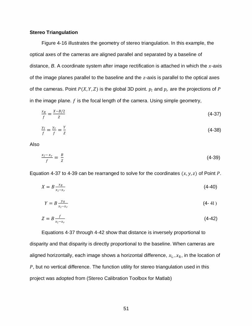
51

Stereo Triangulation

Figure 4-16 illustrates the geometry of stereo triangulation. In this example, the

optical axes of the cameras are aligned parallel and separated by a baseline of

distance, B. A coordinate system after image rectification is attached in which the 𝑥-axis

of the image planes parallel to the baseline and the 𝑧-axis is parallel to the optical axes

of the cameras. Point 𝑃(𝑋,𝑌,𝑍) is the global 3D point. 𝑝𝑙 and 𝑝𝑟 are the projections of 𝑃

in the image plane. 𝑓 is the focal length of the camera. Using simple geometry,

𝑥𝑅

𝑓=

𝑋−𝐵/2

𝑍 (4-37)

𝑦𝑙

𝑓=

𝑦𝑟

𝑓=

𝑌

𝑍 (4-38)

Also

𝑥𝑙− 𝑥𝑟

𝑓=

𝐵

𝑍 (4-39)

Equation 4-37 to 4-39 can be rearranged to solve for the coordinates (𝑥, 𝑦, 𝑧) of Point 𝑃.

𝑋 = 𝐵 𝑥𝑅

𝑥𝑙−𝑥𝑟 (4-40)

𝑌 = 𝐵𝑦𝑅

𝑥𝑙−𝑥𝑟 (4-

𝑍 = 𝐵𝑓

𝑥𝑙−𝑥𝑟 (4-42)

Equations 4-37 through 4-42 show that distance is inversely proportional to

disparity and that disparity is directly proportional to the baseline. When cameras are

aligned horizontally, each image shows a horizontal difference, 𝑥L−𝑥R , in the location of

𝑃, but no vertical difference. The function utility for stereo triangulation used in this

project was adopted from (Stereo Calibration Toolbox for Matlab)

52

Objects at large distance will appear to have no disparity. Since disparity and

baseline are proportional, increasing the baseline will make it possible to detect a

disparity in objects that are farther away. However, it is not always advantageous to

increase the baseline because objects that are closer will disappear from the view of

one or both cameras (Klaus and Horn).

Steps for 3D mapping using stereo vision: The following algorithm gives the

steps to map the fruits in the canopy using stereo vision.

Algorithm 1. Estimation of the intrinsic and extrinsic parameters of the camera

2. Calculation of the Fundamental matrix of the vision system using normalized 8 point algorithm.

3. Image Acquisition using the left and right cameras.

4. Image Rectification of the acquired images

5. Fruit Detection – The fruits in the image are segmented and the image is cleaned for false fruit detection.

6. Ellipse Fitting - An ellipse is fit on the boundary pixels of the fruit and the centroid of the ellipse are obtained

7. Centroid matching of the fruit centroids in the left and right image

8. 3D Mapping of the matched centroids using stereo triangulation algorithm

Step 1 and 2 are done only once for a camera system. Steps 3-8 are repeated each

time the 3D map of the fruits on the image have to be calculated.

In this chapter, the theoretical development and subroutines for 3D mapping using

statistical method and 3D mapping using stereo vision have been described. These

methods are validated performing the four laboratory experiments described in the next

chapter. Figure 4-17 shows the flowchart which summarizes the process of 3D

estimation using stereo vision.

53

A B

Figure 4-1. Effects of radial distortion on image; A) image with radial distortion, B) corrected image

Figure4-2. Comparison of the projection line obtained by PCA and LDA.

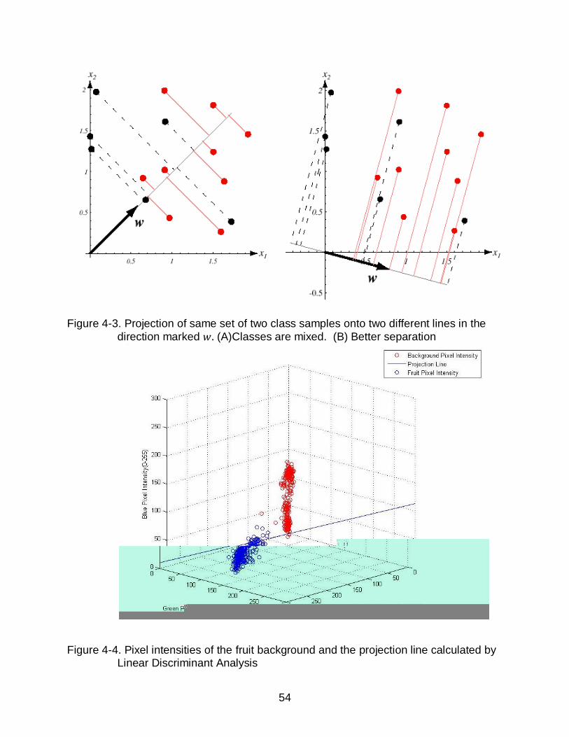
54

Figure 4-3. Projection of same set of two class samples onto two different lines in the

direction marked 𝑤. (A)Classes are mixed. (B) Better separation

Figure 4-4. Pixel intensities of the fruit background and the projection line calculated by

Linear Discriminant Analysis

55

Figure 4-5. Histogram of the dataset pixels projected on 𝑤 (𝑤𝑇𝑥)

A B

C D

Figure 4-6. Original image and their corresponding segmented image A and C show the original RGB image. B and D show the fruits have been segmented using the Linear discriminant analysis.

56

A) B)

C) D)

Figure 4-7. Original Image and the segmented image with Ellipse fit A) and C) are the original Images, B) and D) are the images with Ellipse fit on the detected fruits

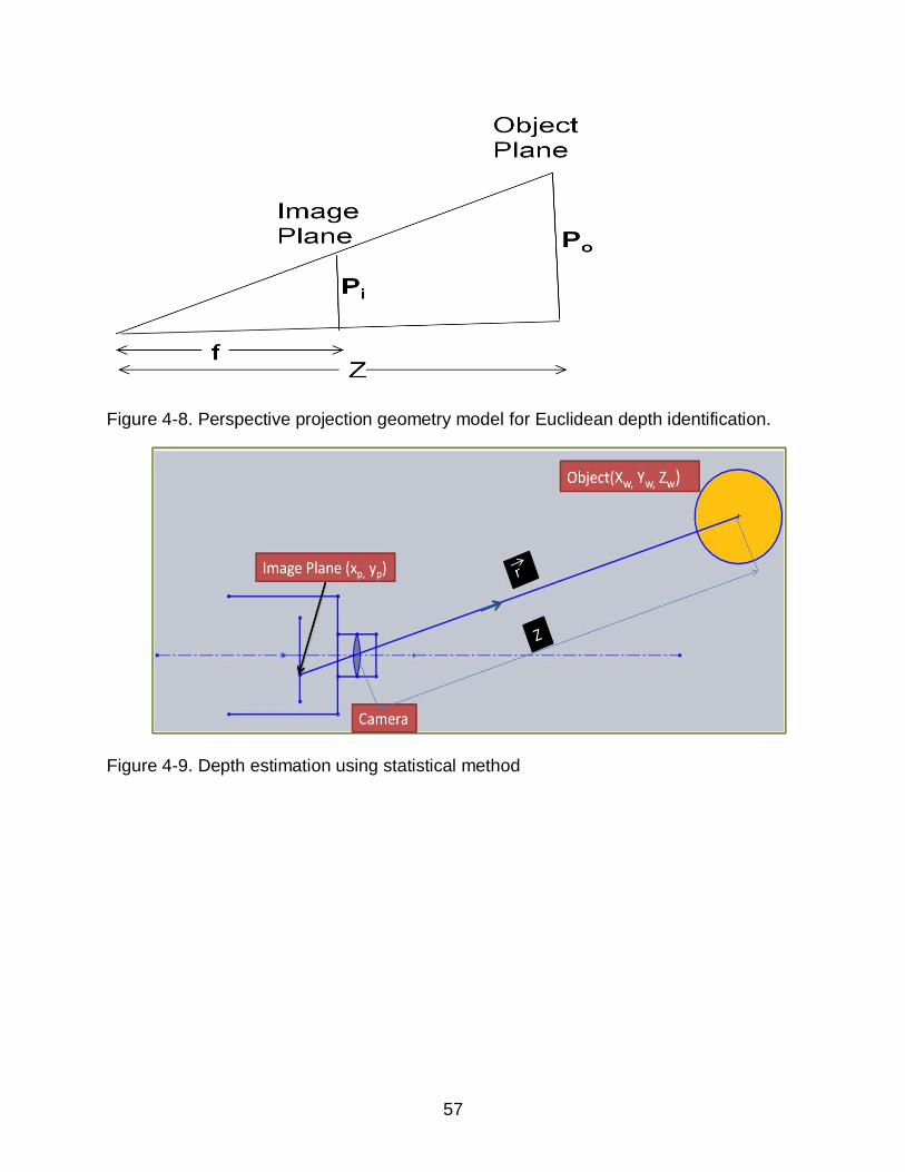
57

Figure 4-8. Perspective projection geometry model for Euclidean depth identification.

Figure 4-9. Depth estimation using statistical method

58

Figure 4-10. Flowchart for 3D point estimation using statistical method.

59

Figure 4-11. Illustration for epipolar geometry

A) B)

Figure 4-12. Matching points used for calculation of Fundamental Matrix A) Points selected in left image shown by red star B) Points selected in right image shown by red star

60

A) B)

Figure 4-13. Images of stereo pair and the epipolar lines A) Points in the left image of the stereo pairB) Corresponding epipolar lines in the right image

Figure 4-14. Image rectification of image planes 𝝅𝑳 and 𝝅𝑹 to 𝝅𝑳′ and 𝝅𝑹′

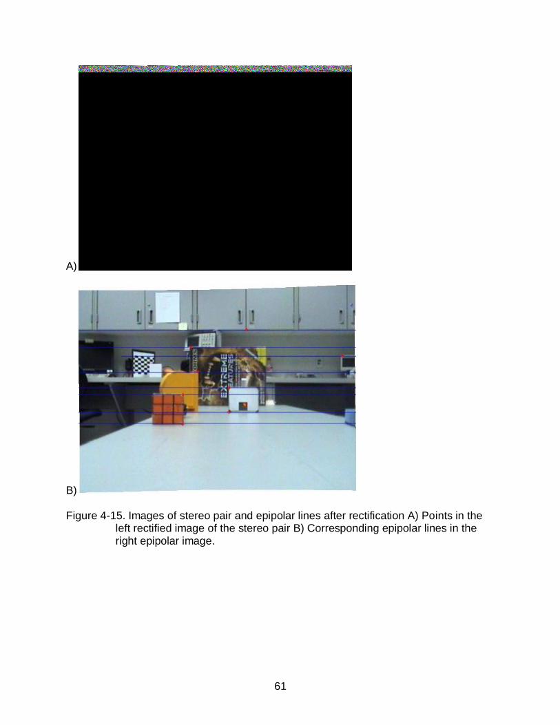
61

A)

B)

Figure 4-15. Images of stereo pair and epipolar lines after rectification A) Points in the left rectified image of the stereo pair B) Corresponding epipolar lines in the right epipolar image.

62

Figure 4-16. Geometry of stereo vision illustrating stereo triangulation

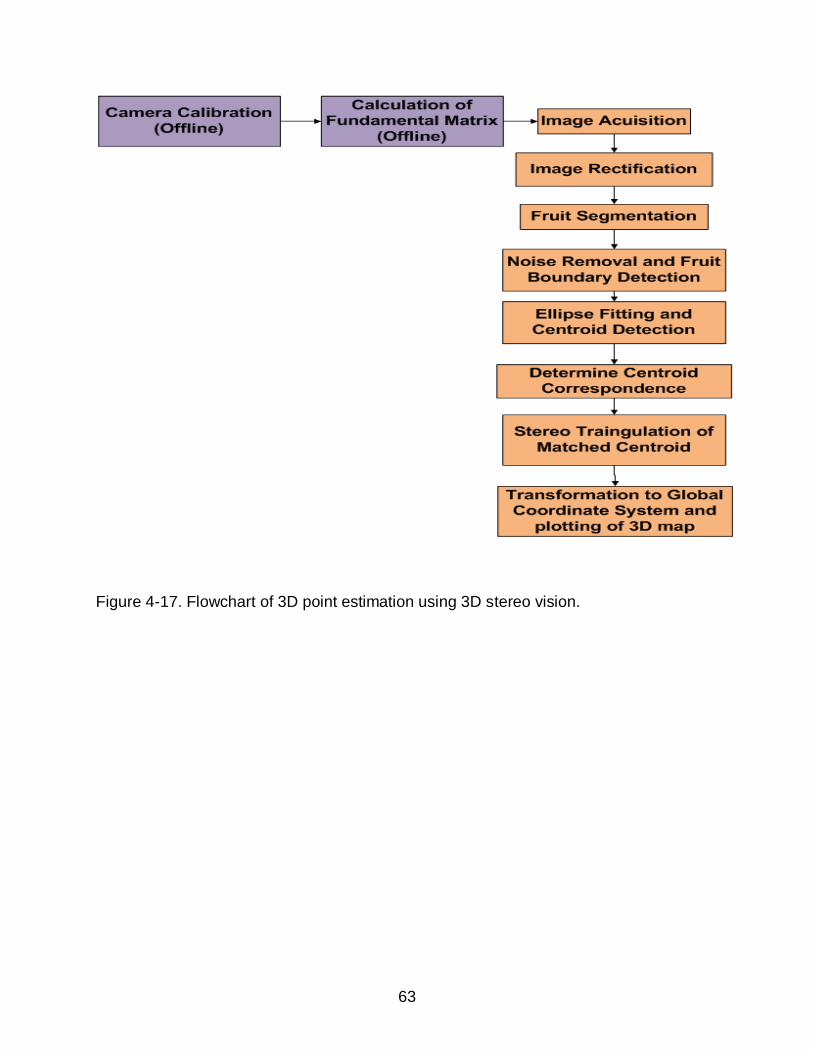
63

Figure 4-17. Flowchart of 3D point estimation using 3D stereo vision.

64

CHAPTER 5

EXPERIMENTS IN 3D MAPPING

Introduction

In this chapter, the experiments to validate the 3D mapping performances using

statistical method and stereo vision are presented. The first section describes the

hardware used in the experiments. The subsequent sections present four different

experiments and their results to validate the robustness of the algorithms.

Hardware Description

The hardware used for the four experiments are the following: (1) vision system,

(2) target objects, (3) robotic manipulator, (4) robot servo controller, (5) three

dimensional measuring system and (6) image processing workstation.

Vision System

The vision system is composed of two identical color CCD cameras (Sony make

Model number: FCB-EX7805) as shown in Figure5-1. The cameras were equipped with

three analog video signals –red, green and blue corresponding to NTSC (National

television system committee) color primaries. The analog signals were digitized with two

frame grabbers (GrabBeeX III audio/video grabber).The cameras are mounted on a

customized frame and it was designed to constrain camera movement in all directions

except along the baseline axis of the cameras for adjustment of the baseline. The view

axis of the left CCD camera was parallel to and as high as the right one. The calibration

of the cameras for the intrinsic parameters was done according to the camera

calibration toolbox for MATLAB. For the extrinsic parameters the camera was calibrated

according to stereo calibration toolbox for MATLAB.

65

Image acquisition was done by setting the cameras simultaneously using a trigger.

The resolution of the images was recorded in 640x480 jpg format. This vision system is

used in both distance estimation methods; for the statistical method, only one of the two

cameras is used.

Target Objects

Two target objects were used for the experiments – Rectangular block and Fake

fruits.

The rectangular block used is shown in Figure 5-2. The dimensions of the

rectangular block are 88mm x 74mm±0.1mm. The rectangular block was used as a

target in Experiment 1 to test the accuracy and robustness of the algorithm at different

depths. Because of its distinct corners, it facilitated in detecting accurate

correspondence in the two images acquired from the vision system for point matching

used in stereo triangulation. In addition, as the rectangular block was accurately

machined it had a definite geometry so its perimeter could be easily calculated.

Fake fruits were used as the target objects in experiments 2, 3 and 4. It was used

as a model of real fruit and to simulate the working of the 3D estimation algorithms with

real fruits. One of the fake fruits used is shown in Figure 5-3. The geometry of the fake

fruits was approximated as an ellipsoid. The fake fruits were not of the same size. The

mean major and minor axis of the fake fruits was calculated by averaging the major and

minor axis of 6 fake fruits and two readings per fruit in direction perpendicular to each

other. The mean semi major axis and semi minor axis of the fake fruit were calculated

as 44.5mm and 37.5mm respectively. The individual fruit data is shown in Table 5-1. In

the 3D estimation using statistical method the mean semi major axis and mean semi

66

minor axis are used to calculate the actual perimeter of the target. This data is used in

3D estimation by statistical method.

Robot Manipulator

The experimental test-bed consists of a Robotics Research K-1607i, a 7-axis,

kinematically-redundant manipulator as shown in Figure. 5-4 The K-1607i model,

offering a 50 inch reach and a 50 lb continuous-duty payload is a lightweight electric-

drive articulated robotic arm.

Robot Servo Controller

The second component of the autonomous citrus mapping testbed is robot servo

control unit. The servo control unit provides a low level control of the robot manipulator

by generating the position/orientation commands for each joint. Robotics Research R2

Control Software provides the low level robot control. The robot controller consists of

two primary components of operation; the INtime real-time component (R2 RTC) and

the NT client-server upper control level component. The R2 RTC provides deterministic,

hard real-time control with typical loop times of 1 to 4 milliseconds. This component

performs trajectory planning, Cartesian compliance and impedance force control,

forward kinematics, and inverse kinematics. The controller can accept commands in the

form of high level cartesian goal points down to low level servo commands of joint

position, torque or current. The network communication between the robot servo control

workstation and the image processing workstation was established using INtime

software by establishing a deterministic and hard real time network communication

control. The servo dynamics of the robot had considerable path errors along all the 7

degrees of freedom and consequently the feedback could not be used for transforming

67

the tool coordinate system to the global coordinates of the robot. As a consequence a

three dimensional measuring system was designed and fabricated.

Three Dimensional Measuring System (TDMS)

A three dimensional measuring system (TDMS) shown in Figure 5-5 was designed

and fabricated to measure the ground truth position of the vision system and targets in

the workspace. The inverse kinematic feedback of the robot was not found to be

accurate to transform the tool frame coordinates into global coordinates of the robotic

manipulator. Multi view 3D mapping of the target required that the tool coordinate of the

robot be transformed into a fixed global coordinate system. The origin of the TDMS

served as a global coordinate system. The vertical distance of the target, along the

negative 𝑌 axis, is measured by a digital laser range finder (Bosch Model number

DLK165K). The frame of the laser range finder can be moved independently along the 𝑋

axis and the 𝑍 axis of the fixed global coordinate system of the TDMS by two lead

screws which are powered by stepper motors (Excitron make Model No.FTFc15). The

resolution of the position of the laser frame along the 𝑋 and 𝑍 axis is 2.5mm. The

resolution of the laser range finder is 1mm. The control program for measurement lead

screw distance travel by stepper motor control is written in Labview.

Image Processing Workstation

The Fourth component is the image processing workstation, which is used for

image acquisition and image processing. The image acquisition and processing is

performed on a Microsoft Windows XP platform based PC with 2.8 GHz Intel Pentium 4

processor and 512 MB RAM.

68

An Intel Open Computer Vision (OpenCV) library is used for image acquisition

from the vision system and the program was developed in Microsoft Visual C++ 6.0. All

the other image processing algorithms were developed in Matlab 7.0.

Experiments Description

Four experiments were conducted to validate the 3D mapping using statistical

method and stereo vision.

Experiment 1

Experimental setup and methodology: The first experiment was performed to

find the 3D estimation of the four corners of the rectangular block by statistical method

and stereo vision. The experimental setup is shown in Figure 5-6. The top view of the

layout experimental setup is shown in Figure 5-7. The vision system was set on a table

and a centerline was drawn parallel to the edges of the table in the direction of the

camera axis. The vision system was placed on the table such that the cameras are

equidistant from the centerline. A scale was marked on the centerline to find the ground

truth in the 𝑍 axis. The scale is calibrated by laser range finder. Translations from the

origin of world coordinate system to the origins of the camera coordinate system were

noted to be:

𝑇𝑙𝑒𝑓𝑡 = −75.9 −64 −10 mm (5-1)

𝑇𝑟𝑖𝑔𝑕𝑡 = 75.9 −64 −10 mm (5-2)

By placing the block sequentially at different distances within the range of 300mm

to 1500mm, 25 images from each camera of the vision system of the rectangular block

were acquired along the centerline at intervals of 50mm. Before acquiring the image at

each interval, it was made sure that the plane of the rectangular block is perpendicular

to the edge of the table using a square.

69

After the image acquisition, the corners in the rectangular block were extracted by

manually selecting the pixel coordinates of the corners of the rectangular block in the 50

images.

Results: The 3D estimation by statistical method uses a single camera. The

selection of camera for this study was done by performance evaluation of 3D estimation

of the corners of the rectangular block using both the cameras independently. The

summary of result of 3D estimation of the corners by statistical method using the left

camera and right camera is tabulated in Table 5-2. The results of both cameras are very

close to each other but the mean of mean percentage error of all the corners over all the

images is slightly lower in the right camera. So in this study, the right camera was

selected for the 3D modeling using statistical method.

Figure 5-9 shows the error plot of 3D estimation of corner 1 by statistical method.

The mean errors at each distance from target to camera are represented by the blue

(for x-axis), red (for y-axis), and green (for z-axis) markings. The error trend line along

the X, Y and Z axis are shown by the blue, red and green lines respectively. From the

error trend lines, the error in estimating distance from target to camera (Z-axis)

increases directly with distance. This result is expected because as the object is moved

farther from the camera, the size of the image decreases which also decreases the

resolution of estimating the distance using the perimeter. The mean absolute error of

corner 1 in the Z direction is 9.36mm and the maximum absolute error was 19.72mm.

The rise in the errors in the X and Y axis are lower than the Z axis. The standard

deviation absolute error of corner 1 over all the distances is 10.95mm.

70

Figure 5-10 shows the error plot for 3D estimation of corner 1 using stereo vision.

The same conventions for plotting of trend lines and mean absolute error are used. The

mean absolute error for estimation of corner 1 along Z direction is 5.02mm. The

Standard deviation of absolute error for corner 1 over all the distances is 5.83mm. Both

these estimates are lower compared to their corresponding value estimated by

statistical method (9.36mm). Similar trends were observed for the other corners.

The summary error plot for the four corners over 25 distance images for statistical

method is shown in Figure 5-11. The results are tabulated in Table 5-3. As expected,

the trend line along the Z direction increases with distance of target from camera. The

increase in trend line along the X and Y directions is lower than error increase in the

distance axis. The mean of mean absolute errors for corners over all 25 distances for

the Z coordinate is 9.25mm and the standard deviation of absolute errors of the four

corners over the 25 distances is 11.42mm. The mean of mean percentage error for the

four corners over all 25 distances in the X, Y and Z directions was observed to be

0.34%, 0.26% and 1.18 %.

Figure 5-12 shows the summary error plot for the four corners over all the

distances for 3D estimation by stereo vision. The results are tabulated in Table 5-4. It is

observed that the mean of mean absolute errors for all corners over all 25 images along

Z direction is 5.34mm. The standard deviation of depth errors is 7.02mm. These error

estimates in stereo vision are lower than estimation by statistical method. The mean of

mean percentage error of the four corners over all 25 distances in the X, Y and Z

directions were observed to be 0.20%, 0.44%and 0.57% which is lower compared to

statistical method.

71

As can be observed in Figure 5-11 and Figure 5-12, comparing the results of both

statistical and stereo vision methods, both distance measuring methods showed an

increase of error in estimation as target was moved farther from the camera. Another

interesting observation was that for the statistical method, the error is below 6.81mm

with standard deviation of 1.57mm within the 300 mm to 800 mm range and then it

starts to increase to 10.76mm with standard deviation of 6.97mm as it moves to 1500

mm. On the other hand, for stereo vision, the error is within 4.57mm with standard

deviation of 2.82mm at a distance of 1250mm and the error is 9.95mm with standard

deviation of 6.13mm as the target is moved to 1500mm. This shows that stereo vision

performed much better over a wider range.

Figures 5-13, 5-14 and 5-15 show the plots between estimated and actual

positions in the x, y and z directions respectively. Since the rectangular block was only

moved along the distance axis, it is expected that the X and Y values should not

change. As expected, from Figure 5-13 and 5-14 the estimated values of X and Y

values are do not show any major deviations from the actual X and Y values, the r-

squared value was calculated between the estimated and actual data. The r-squared

value of 3D estimation along the X, Y and Z axis are 0.9955, 0.9946 and 0.999

respectively.

Figures 5-16, 5-17, 5-18 show the comparison of the actual position and estimated

position of the corners in the X, Y and Z axis respectively by stereo vision. The r-

squared value of 3D estimation along X, Y and Z axis are 0.9971, 0.9885 and 0.9995

respectively. These values imply that the estimated and actual positions are very close

to each other.

72

Figure 5-19 shows the 3D mapping of the actual and estimated positions of the

corners of the rectangular block by statistical method. The left camera is shown by

dotted lines to indicate that it was not used in mapping. The actual position of the

corners at each distance is represented by red crosses and the estimated position is

shown by green crosses. Red and green lines are drawn to connect the corners and

form the perimeter of the rectangular block. Similarly, Figure 5-20 shows the 3D

mapping of the corners by stereo vision. The corresponding red and green corners at all

distances are seen to be very close to each other. In both the figures, the deviation of

estimated corners from the actual corners increases with increase in distance. As

expected, the corresponding crosses are closer to each other for stereo vision.

Experiment 2

Experiment setup and methodology: The experiment setup is shown in Figure

5-21 where four fake fruits were hung from a dummy canopy. Six images were obtained

by translating the camera along the centerline of the table by 50mm interval and made

sure that all four fruits were visible in both the cameras of the vision system. The ground

truth of the fruits was obtained by fixing a string to the base of the fruit and the

projection of the string on the table was marked. The X coordinate was calculated as

the distance from the centerline and the Z coordinate was calculated by projecting the

marked point on the centerline and measuring the distance of projection of the

centerline from origin on the scale drawn on centerline. The Y coordinate is calculated

by laser range finder to the base of the fruit and adding the length of semi major axis of

the fruit.

73

Results: Figure 5-22 shows the error plot of 3D estimation of fruit 1 by statistical

method. The mean absolute error in the Z axis increases with distance of vision system

from the canopy. The mean absolute error in depth was 17.98mm.

The mean absolute error is higher than the error obtained in experiment 1. The reason

could be that unlike the rectangular block, the fake fruit does not have a standard

geometry. The geometry of the fake fruit has been approximated as an ellipsoid with

known major and minor axis as shown in Table 5-1. Moreover, the projection of the fake

fruit on the image is also considered to be an ellipse to calculate the centroid of the fruit.

These reasons could possibly explain the increase in error in 3D position estimation by

statistical method when fake fruit was used as target compared to using the rectangular

block which had standard geometry.

Figure 5-23 shows the error plot of fruit 1 by stereo vision. The mean absolute

error in depth was 17.42mm. In this case too, the mean absolute error is higher than in

experiment 1. Stereo vision calculates the error by triangulation principle. The same

feature has to be detected on both the images; For experiment 1, the corners of the

rectangular block are sharp and distinguishable in both the images. However in case of

fake fruit, the centroid of the fake fruit detected depends on the projection of the fake

fruit in both the images and the performance of the segmentation algorithm. The

mismatching of pixels as fruit centroids can lead to increase in error in stereo

triangulation.

The summary error plot for the 4 fruits over the 6 images for statistical method is

shown in Figure 5-24. The results are tabulated in Table 5-5. The mean of mean

absolute errors of the 4 fruits over all the 6 distances is 28mm and the standard

74

deviation of the depth errors 4 fruits in the 6 distances is 33mm. The mean of mean

percentage error in a given direction was calculated as the mean of mean absolute error

of the 4 fruits in all 6 images in that given direction to the average depth of all 4 fruits in

all 6 images. This value in the X, Y and Z directions were observed to be 0.96%, 0.87%

and 2.43%, respectively. It was interesting to note that the error in Z direction of fruit 3

was higher than the other fruits. The reason could be that apart from being the farthest

fruit from the camera, it was partially occluded by fruit 2 in the images. A separation was

created between the fruits manually in the image, so the entire projection of the fruit was

not seen in the images.

Figure 5-25 shows the summary error plot for the 4 fruits over all the 6 images

from each camera for 3D estimation using stereo vision. The results are tabulated in

Table 5-6. It is observed that the mean of mean absolute errors in all 4 fruits in the 6

images for the Z coordinate is 18.16mm. The standard deviation of depth errors over

the 6 images and corners is 5.15mm. The mean of mean percentage error in depth is

calculated to be 1.76%. The mean error estimates and standard deviation are lower

compared to the errors obtained by statistical method. As expected, the trend lines in

Figure 5-24 and Figure 5-25 rise with distance of the target scene from the camera. The

error values are higher than the summary plots of experiment 1. As explained in the

description of errors in fruit 1, the reason could be the ambiguous geometry of the fake

fruit compared to the rectangular block, and mismatching of pixels as fruit centroids

because of the different projections in the left and right cameras.

Figures 5-26, 5-27 and 5-28 show the plot of the estimated 3D position by

statistical method to actual global position in the X, Y and Z directions respectively of

75

the 4 fruits in the 6 images acquired for experiment 2. In Figure 5-26 and Figure 5-27

there are 4 clusters of six points showing the corresponding X and Y position in each

image. This is expected because the X and Y positions of the fruit are not changing

when the vision system is translated along the Z direction for each reading. The r

squared value is 0.9832, 0.9842 and 0.9859 in the x, y and z directions respectively.

Figure 5-29, 5-30 and 5-31 show the plot of the estimated to actual global position

of 4 fruits in 6 images by stereo vision. Similar to Figure 5-26 and Figure 5-27, here too

the 4 clusters of six points are observed. The r squared value in the X, Y and Z

directions are 0.9882, 0.9938 and 0.9937 respectively. The r squared vales obtained by

both the methods are close to unity which indicates the performance of both the

algorithms is very good. Again r squared values in 3D estimation using stereo vision are

closer to unity than 3D estimation by statistical method

In Figure 5-32 (A) to 5-32 (F) the 3D map of the fruits using statistical method is

shown. It is arranged with sequentially increasing distance of vision system from the

canopy. Actual 3D location is represented by orange spheres and the estimated 3D

position is represented by gray spheres. The arrangement of the fruits in the map is

similar to the actual orientation of the fruits in the experiment shown in Figure 5-21. As

expected, significant overlap between the fruits in the images is noted. In Figure 5-32(F)

which is when the fruit was farthest from the vision system, there is low overlap in fruit 3

due to relatively higher error in estimating depth. The reason has been explained above.

Similarly, Figures 5-33 (A) to Figure 5-33(F) shows the 3D map of fake fruits in

experiment 2 by stereo vision arranged sequentially from increasing distance of vision

system from the canopy. Here too, significant overlap is observed between the

76

estimated and actual position of the fruits in the canopy. The orientations of the fruits in

the map are also observed to be similar to the fruit orientations in the experiment setup

shown in Figure 5-21.

Figure 5-34 shows a consolidated 3D map using statistical method combining the

3D maps from all the six views in a fixed camera coordinate system. Similarly the

concatenated 3D map using stereo vision is shown in Figure 5-35. We observe that

there is no major deviation in any of the estimated position from the actual position of

the fruit. The orientation of the fruits is similar to the experimental setup.

Experiment 3

Experiment setup and methodology: As reviewed earlier, viewing the canopy

from multiple perspectives increases the visibility of fruits in the canopy. This

experiment was done to test the effect of multi view mapping on estimation of 3D

position. The experimental setup is shown in Figure 5-35. The vision system was

mounted as the end effecter of the robot manipulator. A single fake fruit is hung in the

canopy. Images of the fruit were acquired from 5 different arbitrary views of the vision

system. Before taking the images from a given position of the vision system it was made

sure that the coordinate system of the TDMS was aligned to the axes of the vision

system by using electronic level. The translation of the vision system for each of the

views is measured by TDMS. The ground truth location of the fruit is also measured by

TDMS.

Results: Table 5-7 summarizes the results of 3D estimation of a single fake fruit in

the canopy fruit using multiple views by statistical method. The results are similar to the

results performed in experiment 2 by statistical method. The mean absolute error in the

z axis is 25.16mm and the standard deviation in depth is 12.9mm. The percentage error

77

along the X, Y and Z axis are observed to be 1.42%, 1.54% and 3.03% respectively.

Figure 5-35 (A)-(F) show the 3D maps of the single fruit generated from each view. The

blue spheres represent the actual position and the yellow spheres represent the

estimated position. It can be observed that there is considerable overlap between the

spheres in all the images. This shows that the algorithm is robust to translation in the

plane of the camera. The consolidated map combining all the five views from statistical

method is shown in Figure 5-37 with respect to fixed origin of TDMS. The translation of

the camera system with respect to the origin is also shown. The left camera of the vision

system which is not used in statistical method is represented by red dotted line. From

the figure it is observed that all the views produce a good estimate for mapping of the

fruit.

Table 5-8 summarizes the results of the 3D estimation of the fruit using multiple

views by stereo vision. The mean percentage error in the X, Y and Z directions were

calculated to be 0.92%, 1.45% and 1.34%. The results show an improved performance

in estimation of fruit targets using stereo vision.

It can be observed that there is some increase in the error compared to

experiment 2. The vision system was aligned to the TDMS before taking the image for

every view using electronic level. The electronic level had resolution of 0.1 degree. The

alignment errors between the vision system and TDMS can cause increase in the

overall error.

Figure 5-36 (A)-(F) shows the 3D map of the estimated position and actual

position of the fake fruit from each perspective relative to origin of the TDMS. The

consolidated map from the five views of stereo vision is shown in Figure 5-38. Again,

78

the fruit map shows that the estimated 3D position is a very good approximation of the

actual 3D position. The consolidated map in Figure 5-38 shows the five perspectives of

the camera positions and the calculated position of the fruit. The estimated position of

the fruit position matches closely with the approximated position. The lower standard

deviation in estimation by stereo vision can also be observed from Figure 5-38 and

Figure 5-29 by the lesser spread of the yellow color in the consolidated maps.

Experiment 4

Experimental Methods and Methodology: This experiment was done to test the

effect of multi view perspective when there are multiple targets on the scene. The

experimental setup is shown in Figure 5-39. Three fruits were hung in the canopy and

their 3D positions were calculated by TDMS. The methodology of the experiment was

similar to experiment 3. Images of the fruits were taken from 5 perspectives of the vision

system. The translation of the vision system for each perspective of the TDMS was

noted. It was made sure that all the fruits were visible in both the cameras of the vision

system in all the 5 perspectives. Translation of the vision system for each perspective

and the ground truth of the fruit were measured by TDMS. Before taking images from a

perspective it was made sure that the coordinate axis of the vision system was aligned

with the coordinate axis of the TDMS by using electronic level.

Results: The results for experiment 4 by statistical method are summarized in

Table 5-9. The mean absolute errors of the fruits are in the expected range for fake

fruits obtained in experiment 2. The mean of mean percentage error of the three fruits in

all the five views along the distance axis is 4.55%. Along the X and Y axis, the value is

2.28% and 2.33%. The observed error was higher than the observed errors in

experiment 2 and 3. The fruits in this experiment were more hidden as compared to

79

experiments 2 and 3. Along with taking into account the alignment errors in the views,

the error in fruit segmentation because of partial occlusion by leaves could be the

reason for increase in error. The 3D mapping by statistical vision using each of the

perspectives individually is shown in Figure 5-40. It can be seen that the arrangement of

fruits in the map is similar to the actual arrangement in the experiment setup. This

shows that the estimates of 3D position are correct.

Table 5-10 shows the summary of results of experiment 4 by stereo vision. The

accuracy of stereo vision is better than statistical method in this experiment too. The

overall percentage error is 1.76% and 1.70% in the X and Y axis and 1.99% in the Z

direction. These error values are what expected based on experiment 2 and 3 are. The

single perspective plot for each view is shown in Figure 5-41. Here again the similarity

of arrangement of the estimated position and the arrangement in actual setup can be

seen. The consolidated multi-perspective 3D map by statistical method and stereo

vision is shown in Figure 5-42 and Figure 5-43 respectively. From both the

consolidated maps it can be observed that the estimated 3D position closely maps the

actual 3D position of the fruit.

80

Table 5-1. Size data of fake fruit used as target fruits.

Mean major axis (mm) Mean minor axis (mm)

Fruit 1 87.5 72.3

Fruit 2 89.8 75.3

Fruit 3 90.2 74.9

Fruit 4 90.1 75.3

Fruit 5 87.6 77.3

Mean (mm) 89.04 75.02

Standard deviation (mm) 01.37 01.79

Table 5-2. Summary of the 3D estimation of corners of the rectangular block in experiment 1 by statistical method using left camera

Camera in the Vision system

Mean of mean percentage error in X(mm)

Mean of mean percentage error in Y(mm)

Mean of mean percentage error in Z(mm)

Left Camera 0.4567 0.3362 1.1977

Right Camera 0.3498 0.2669 1.1883

81

Table 5-3. Summary of results of 3D estimation of corners of rectangular block in experiment 1 using statistical method

Axis

Mean Absolute Error corner1 (mm)

Mean Absolute Error corner2 (mm)

Mean Absolute Error corner3 (mm)

Mean Absolute Error corner4 (mm)

Mean of Mean Absolute Error(mm)

Standard Deviation of Errors(mm)

Mean of Mean Percentage Error(%)

X 2.6537 1.1163 2.13 2.7167 2.1542 2.8696 0.3498 Y 1.5158 2.4607 2.4664 2.4498 2.2232 2.3563 0.2669 Z 9.3673 9.0484 7.8654 10.7284 9.2524 11.4261 1.1883

Table 5-4. Summary of results of 3D estimation of corners of rectangular block in experiment 1 using stereo vision

Mean Absolute Error corner1 (mm)

Mean Absolute Error corner2 (mm)

Mean Absolute Error corner3 (mm)

Mean Absolute Error corner4 (mm)

Mean of Mean Absolute Error(mm)

Standard Deviation of Errors(mm)

Mean of Mean Percentage Error(%)

X 1.0927 2.3085 2.7229 1.0863 1.8026 2.0056 0.2096 Y 2.4741 2.6726 4.3082 4.7978 3.5632 1.5008 0.4491 Z 5.0285 5.8637 3.9171 6.4128 5.3055 7.0292 0.5738

Table 5-5. Summary of results of 3D estimation of experiment 2 using statistical method

Coordinate Axis

Mean Absolute Error Fruit1 (mm)

Mean Absolute Error Fruit2 (mm)

Mean Absolute Error Fruit3 (mm)

Mean Absolute Error Fruit4 (mm)

Mean of Mean Absolute Error(mm)

Standard Deviation of Mean error(mm)

Standard Deviation of Errors(mm)

Mean of Mean Percentage Error in depth(%)

X 16.6808 1.2563 15.9056 13.5384 11.8453 1.863 7.386 0.96 Y 8.8549 5.9206 21.0794 6.247 10.5255 1.081 6.504 0.87 Z 17.9811 2.0551 47.7899 16.7502 28.6441 10.337 33.33 2.43

83

Table 5-9. Results table for experiment 4 by statistical method

Axis Mean Error Fruit1 (mm)

Mean Error Fruit2 (mm)

Mean Error Fruit3 (mm)

Mean of Mean Absolute Error(mm)

Standard Deviation of Errors(mm)

Mean Percentage Error(%)

X 19.1626 11.6738 12.2193 14.3519 2.8696 2.28 Y 11.8822 12.8548 19.2319 14.6563 2.3563 2.33 Z 25.8788 38.2189 21.9345 28.6774 11.4261 4.55

Table 5-10. Results table for experiment 4 by stereo vision

Axis Mean Error Fruit1 (mm)

Mean Error Fruit2 (mm)

Mean Error Fruit3 (mm)

Mean of Mean Absolute Error(mm)

Standard Deviation of Errors(mm)

Mean Percentage Error(%)

X 13.9275 10.6839 8.5873 11.0662 7.1262 1.76 Y 8.5899 8.8148 14.71 10.7049 3.1927 1.70 Z 14.5508 17.7482 5.3937 12.5642 7.0527 1.99

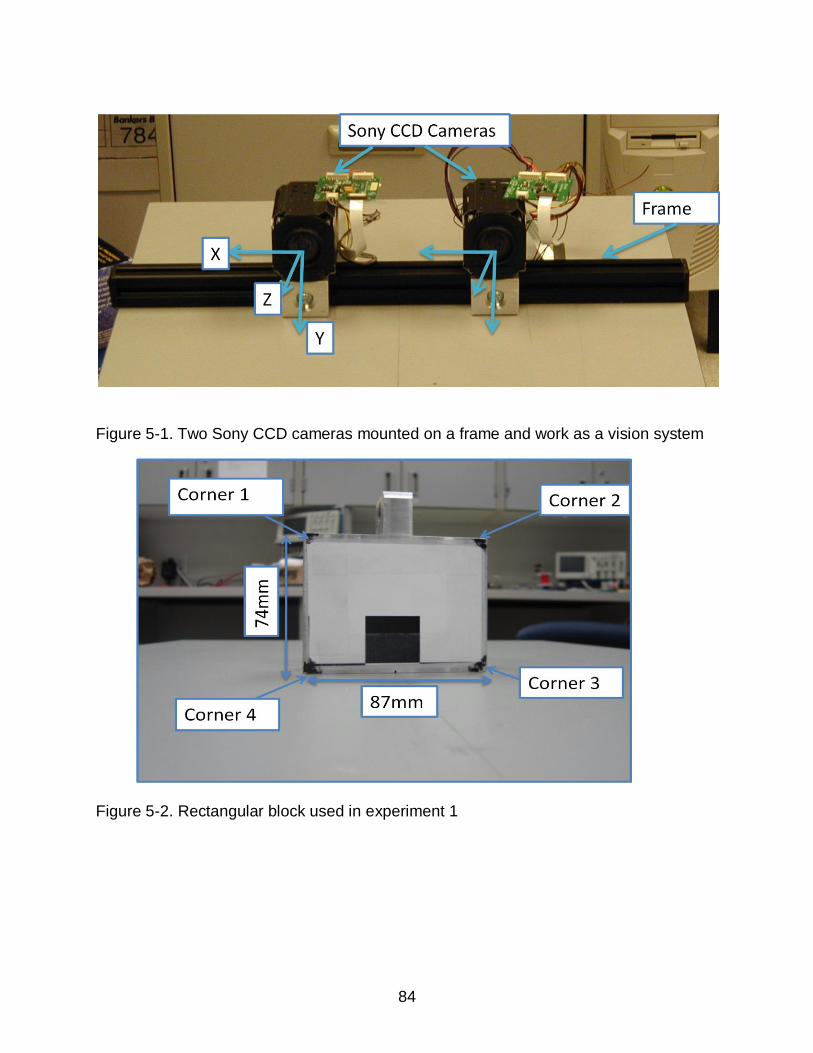
84

Figure 5-1. Two Sony CCD cameras mounted on a frame and work as a vision system

Figure 5-2. Rectangular block used in experiment 1

85

Figure 5-3. Fake fruit used as a target object

86

Figure 5-4. Robotics Research K-1607i, a 7-axis, kinematically-redundant manipulator

Figure 5-5. Three dimensional measuring system

87

Figure 5-6. Experimental setup for experiment 1

Figure 5-7. Top view of experimental setup of experiment 1

88

Figure 5-9. Error plot for corner 1 by statistical method

Figure 5-10. Error plot for corner 1 by stereo vision

89

Figure 5-11. Summary plot of experiment 1 by statistical method

Figure 5-12. Summary plot of experiment 1 by stereo vision

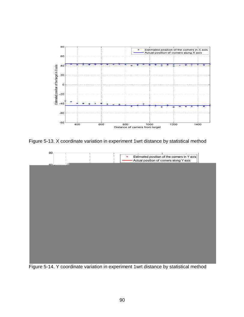
90

Figure 5-13. X coordinate variation in experiment 1wrt distance by statistical method

Figure 5-14. Y coordinate variation in experiment 1wrt distance by statistical method

91

Figure 5-15. Z coordinate variation in experiment 1 wrt distance by statistical method

Figure 5-16. X coordinate variation in experiment 1wrt distance by stereo vision

92

Figure 5-17. Y coordinate variation in experiment 1wrt distance by stereo vision

Figure 5-18. Z coordinate variation in experiment 1wrt distance by stereo vision

93

Figure 5-19. 3D reconstruction plot of the corners of the rectangular block by statistical method

Figure 5-20. 3D reconstruction plot of the corners of the rectangular block by stereo vision

94

Figure 5-21. Test setup of experiment 2

Figure 5-22. Error plot for fruit 1 by statistical method

95

Figure 5-23. Error plot for fruit 1 by stereo vision

Figure 5-24. Summary error plot for fruit 1 by statistical method

97

Figure 5-27. Scatter plot for the estimated Y coordinate of the fruits wrt actual Y coordinate by statistical method

Figure 5-28. Scatter plot for the estimated Z coordinate of the fruits wrt actual Z coordinate by statistical method

98

Figure 5-29. Scatter plot for the estimated X coordinate of the fruits wrt actual X coordinate by stereo vision

Figure 5-30. Scatter plot for the estimated Y coordinate of the fruits wrt actual Y coordinate by stereo vision

99

Figure 5-31. Scatter plot for the estimated Z coordinate of the fruits wrt actual Z coordinate by stereo vision

100

A

Figure 5-32. 3D map of fake fruits in canopy of experiment 2 by statistical method. (A)-(F) represent the map of six views taken increasing the distance of vision system from the canopy.

A

B

C D

E F

101

Figure 5-33. 3D map of fake fruits in canopy of experiment 2 by stereo vision. (A)-(F) represent the map of six views taken increasing the distance of vision system from the canopy.

A B

C D

E F

102

Figure 5-32. Consolidated 3D map of all 6 views using statistical method

Figure 5-33. Consolidated 3D map of all 6 views using stereo vision

103

Figure 5-34. Test setup for experiment 3

104

Figure 5-35. Single perspective 3D map estimation of fruit in experiment 3 by statistical method

A B

C D

E

105

Figure 5-36. Single perspective 3D map estimation of fruit in experiment 3 by stereo vision

A B

C D

E

106

Figure 5-37. Multiperspective 3D map of target in experiment 3 by statistical method

Figure 5-38. Multiperspective 3D map of target in experiment 3 by stereo vision

107

Figure 5-39. Test setup for experiment 4

108

Figure 5-40. Single perspective 3D map estimation of targets in experiment 4 by

statistical method

A B

C D

E

109

Figure 5-41. Single perspective 3D map estimation of targets in experiment 4 by

stereo vision

A B

C D

E

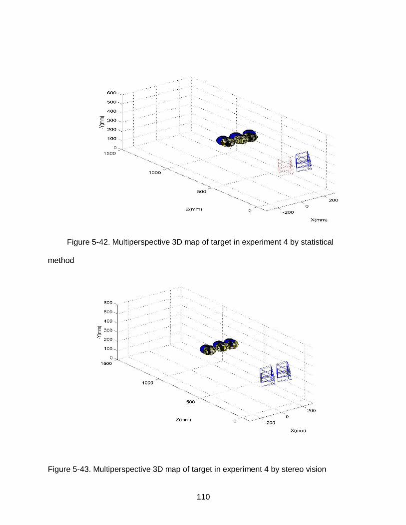
110

Figure 5-42. Multiperspective 3D map of target in experiment 4 by statistical

method

Figure 5-43. Multiperspective 3D map of target in experiment 4 by stereo vision

111

CHAPTER 6 CONCLUSION

3D maps of citrus fruits using computer vision was developed using two methods –

statistical method and stereo vision. A vision system consisting of two cameras was

built to acquire images of targets of known 3D position in laboratory experiments. The

performance of the methods was compared in the range of 300mm to 1500mm of target

and different positions of the targets in the image. Two targets were used for testing the

algorithm- A rectangular block of known dimensions and fake fruits. The following are

the conclusions that were derived from this study:

1. 3D map by statistical method was found to be feasible. First, 3D map by statistical method was developed for the mapping corners of rectangular block of known dimensions at distances in the range of 300mm to 1500mm. The error along the distance axis was 1.18% and the error along the X and Y axis were 0.34% and 0.26% respectively. Then, the algorithm was used to map fake fruits by moving the vision system at 6 distances from the canopy with fruit distances in the range of 650 mm to 1450mm. The error along the distance axis was observed to be 2.43% and the error along X and Y axis were observed to be 0.52% and 0.63%. Then 3D mapping using multiple perspectives was implemented on a single fruit and 3 fruits in the image by mounting the vision system on 1607 robot manipulator. The errors along the distance axis were found to be 3.03% and 1.42% and 1.54% along the X, Y and Z axis for a single fruit respectively.

2. 3D map based on stereo vision was also found to be a viable option. Performance of stereo vision on mapping the corners of the rectangular block along the distance axis was found to be accurate up to 0.57% and the error along the X and Y axis was 0.2% and 0.44% respectively. When the algorithm was tested with fake fruits at different distances of canopy from vision system the error along X, Y and Z axis were 0.53%, 0.63% and 1.76%, respectively. The performance of 3D mapping of target fruits using multi perspective mapping of single fruit had accuracy of 0.92%, 1.45% and 1.34% in X, Y and Z axis respectively.

3. Comparing the performance of both methods, the stereo vision performed better than statistical method. The stereo vision had lower error in the X, Y, and Z directions and the increase in error with increase in distance was lower for the stereo vision. However, based on the results, both methods have the potential for 3D mapping of fruits in the canopy. Both have its advantages and disadvantages. The stereo vision method has a more accurate 3D mapping representation of the

112

targets but it has a higher complexity in hardware implementation. The two cameras that form a stereo pair have to be precisely mounted and calibrated accurately. For any change in the positions of the two cameras which can be caused because of repetitive operation, the vision system has to be recalibrated. In addition, the stereo vision system requires the target to be visible in both images of the vision system. In addition, it is computationally more burdensome than statistical method. On the other hand, the statistical method is easier to implement with only one camera but it has lower accuracy in 3D mapping. Statistical method assumes the shape and size of the fruit to be constant for mapping. If the size or shape variation in fruits is high, the 3D position estimates would not be accurate. Similarly, partial fruit occlusion would cause the error estimates to increase. On the contrary, 3D estimation using stereo vision would be immune to these cases if the reasonable estimate of the centroid of the fruit is obtained.

4. Fruit detection based on Linear Discriminant analysis was found to work well in lab conditions for detecting fruits from the background and was compatible with both the methods. There were observed false detections when the background color was similar to the fruit and when the fruit was saturated. The Ellipse fitting algorithm was found to work robustly with both methods and was successful in detecting the centroid and the perimeter of the detected fruit when the boundary of the fruit was detected properly.

Future Work

The results of this study have shown the feasibility of creating a 3D map for target

objects in a scene using statistical method and stereo vision method. However, further

studies are needed to warrant its practical application for fruit harvesting. The following

are future studies that need to be conducted:

1. Field test of the current vision system and algorithm. The outdoor grove provides more challenges in terms of variability in illumination and fruit arrangement. The robustness of the algorithm in outdoor conditions has to be verified.

2. Improvement of the fruit detection method and ellipse detection. As observed in the results of fruit segmentation, there were some false detection when the color of the background was similar to the fruit color and when the fruit was saturated. Therefore a quantitative performance evaluation of fruit segmentation is needed especially in outdoor conditions where illumination variability and unstructured fruit positions are present. In addition, the developed ellipse fitting works well for well defined single fruit, however in the field, occlusion and fruits in cluster are challenges that need to be solved.

3. 3D map update process. During actual harvesting, the 3D maps need to be updated due to unloading of the canopy and movement of unharvested fruits to

113

new position. Even during the harvesting operation there are possibilities to detect new fruits. To increase harvest efficiency, the 3D map has to be robust enough to account for the newly detected fruit.

4. Development of path planning for fruit harvesting. Once a 3D map of the tree canopy is developed, a path planning approach should be developed to improve fruit harvest efficiency.

114

APPENDIX LIST OF MATLAB CODES

Fruit Segmentation by Linear Discriminant analysis function [w] = LDAplane (data, label, test) %Inputs: data of fruit and background, label as fruit and background, Test data %Output: One dimensional vector w. data=data'; featNum=size(data,1); dataNum=size(data,2); for Nclass=min(label):max(label) classLabel=(label==Nclass); for k=0:1 % Load digits x=data(:,find(classLabel==k)); eval(['x',num2str(k),'=x;']); %mean mui(:,end+1)=mean(x,2); end mu=mean(mui,2); %covariance covW=0; covB=0; for k=0:1 eval(['x=x',num2str(k),';']); for n=1:size(x,2) covW=covW+(x(:,n)-mui(:,k+1))*(x(:,n)-mui(:,k+1))'; end end covW=covW/dataNum; %normal vector to Hyperplane classW=-inv(covW)*diff(mui,1,2); %offset w(:,end+1)=classW; end hold on;scatter3(data(1,1:275),data(2,1:275),data(3,1:275),'r'); line([-w(1,2)*500 w(1,2)*500],[-w(2,2)*500 w(2,2)*500],[-w(3,2)*500 w(3,2)*500]) hold on; scatter3(data(1,276:size(data,2)),data(2,276:size(data,2)),data(3,276:size(data,2)),

'b') view(142,32) proj_frt = dot(data(:,276:550),repmat(w(:,1),[1 275])); proj_canopy = dot(data(:,1:275),repmat(w(:,1),[1 275])); figure; hist(proj_frt,20); h = findobj(gca,'Type','patch'); hold on;

115

hist(proj_canopy,20); set(h,'FaceColor','r','EdgeColor','w') proj_frt1 = dot(test(:,276:550),repmat(w(:,1),[1 275])); proj_canopy1 = dot(test(:,1:275),repmat(w(:,1),[1 275])); figure; hist(proj_frt1,20); h = findobj(gca,'Type','patch'); hold on; hist(proj_canopy1,20); set(h,'FaceColor','r','EdgeColor','w') return Elliipse fitting algorithm

function [semimajor_axis, semiminor_axis, x0, y0, phi] = ellipse_fit(x,y) % ellipse_fit - Given a set of points (x,y), ellipse_fit returns the % best-fit ellipse (in the Least Squares sense) % Input: % x - a vector of x measurements % y - a vector of y measurements % % Output: % semimajor_axis - Magnitude of ellipse longer axis % semiminor_axis - Magnitude of ellipse shorter axis % x0 - x coordinate of ellipse center % y0- y coordinate of ellipse center % phi - Angle of rotation in radians with respect to % the x-axis x = x(:); y = y(:); %Construct M M = [2*x.*y y.^2 2*x 2*y ones(size(x))]; % Multiply (-X.^2) by pseudoinverse(M) e = M\(-x.^2); %Extract parameters from vector e a = 1; b = e(1); c = e(2); d = e(3); f = e(4); g = e(5); delta = b^2-a*c; x0 = (c*d - b*f)/delta; y0 = (a*f - b*d)/delta; phi = 0.5 * acot((c-a)/(2*b)); nom = 2 * (a*f^2 + c*d^2 + g*b^2 - 2*b*d*f - a*c*g); s = sqrt(1 + (4*b^2)/(a-c)^2);

116

a_prime = sqrt(nom/(delta* ( (c-a)*s -(c+a)))); b_prime = sqrt(nom/(delta* ( (a-c)*s -(c+a)))); semimajor_axis = max(a_prime, b_prime); semiminor_axis = min(a_prime, b_prime); if (a_prime < b_prime) phi = pi/2 - phi; end 3D estimation of corners of rectangular block by statistical method

clc clear T_right = [75.9 ;-64;-10]; T_left = [- 75.9;-64; -10]; % load Calib_Results_stereo.mat for k=1:25 %for rectified images z=1550-50*k; dp(k)=1550-50*k; G(:,1,k)=[-44;-74.12;z]; G(:,2,k)=[44;-74.12;z]; G(:,3,k)=[44;0;z]; G(:,4,k)=[-44;0;z]; end sqv = 87.8;sqh = 74; Pmact =2*(sqv+sqh); load corner_dist.mat; KK_right = [969.9471 0 320.6631 0 978.2932 240.2693 0 0 1.0000]; KK_left =[ 969.9471 0 320.6631 0 978.2932 240.2693 0 0 1.0000] xR(3,:,:)=1;xL(3,:,:)=1; for i=1:25 Pm1(i)= 2*(norm(xR(1:2,2,i) - xR(1:2,3,i)) + norm(xR(1:2,4,i) - xR(1:2,3,i))); d1(i) = 862*Pmact/Pm1(i); end d=d1; X = [1500:-50:300]; for i=1:25 for j=1:4 r1 = KK_right \ xR(:,j,i); r1 =r1/norm(r1); x3d1(:,j,i) = d(i)*r1; r2 = KK_left \ xL(:,j,i); r2 =r2/norm(r2); x3d2(:,j,i) = d(i)*r2; end

117

end TR = repmat(T_right,[1,size(x3d1,2),size(x3d1,3)]); TL = repmat(T_left,[1,size(x3d2,2),size(x3d2,3)]); Pos_r = TR+x3d1; Pos_l =TL+x3d2; Pos = (Pos_r +Pos_l )/2; a=1.294/2; Ry = [cosd(a) 0 sind(a);0 1 0;-sind(a) 0 cosd(a)]; for i=1:25 Pos1(:,:,i) = Pos_r(:,:,i);%(Pos_r(:,:,i)+Pos_l(:,:,i))/2; end err= G-Pos1; newplot1(G,Pos1); % plot_indcorners(err); % plot_err(err); 3D estimation by stereo vision

function stereo_check %Definition of parameters wrt global frame T_left = [- 75.9;-64; -10]; T_right = [ 75.9 ;-64; -10]; Cam_dist=155.5; load Calib_results_stereo.mat; load Calib_results_stereo_rectified % load datnorect.mat load corner.mat; for k=1:25 %for rectified images z=1550-50*k; G(:,1,k)=[-44;-74;z]; G(:,2,k)=[44;-74;z]; G(:,3,k)=[44;0;z]; G(:,4,k)=[-44;0;z]; xL1 = xL(:,:,k); xR1 =xR(:,:,k); [XL,XR] = stereo_triangulation(xL1,xR1,om_new,T_new,fc_left_new

,cc_left_new ,kc_left_new ,alpha_c_left_new ,fc_right_new ,cc_right_new ,kc_right_new ,alpha_c_right_new );

GL = XL+repmat(T_left,1,size(XL,2)); GR = XR+repmat(T_right ,1,size(XR,2)); EGLGR(:,:,k) = GR-GL; G1(:,:,k) =(GL+GR)/2; end a= -1.294/2; Ry = [cosd(a) 0 sind(a);0 1 0;-sind(a) 0 cosd(a)]; for i=1:25 Pos1(:,:,i) = Ry* G1(:,:,i) end

118

err = Pos1-G; err plot_indcorners(err); plot_err(err) % newplot1(G,Pos1); a=1; Stereo triangulation available in camera calibration toolbox function [XL,XR] =

stereo_triangulation(xL,xR,om,T,fc_left,cc_left,kc_left,alpha_c_left,fc_right,cc_right,kc_right,alpha_c_right),

% [XL,XR] = stereo_triangulation(xL,xR,om,T,fc_left,cc_left,kc_left,alpha_c_left,fc_right,cc_right,kc_right,alpha_c_right),

% % Function that computes the position of a set on N points given the left and right

image projections. % The cameras are assumed to be calibrated, intrinsically, and extrinsically. % % Input: % xL: 2xN matrix of pixel coordinates in the left image % xR: 2xN matrix of pixel coordinates in the right image % om,T: rotation vector and translation vector between right and left

cameras (output of stereo calibration) % fc_left,cc_left,...: intrinsic parameters of the left camera (output of stereo

calibration) % fc_right,cc_right,...: intrinsic parameters of the right camera (output of

stereo calibration) % Output: % XL: 3xN matrix of coordinates of the points in the left camera reference

frame % XR: 3xN matrix of coordinates of the points in the right camera reference

frame % Note: XR and XL are related to each other through the rigid motion equation:

XR = R * XL + T, where R = rodrigues(om) % For more information, visit

http://www.vision.caltech.edu/bouguetj/calib_doc/htmls/example5.html % (c) Jean-Yves Bouguet - Intel Corporation - April 9th, 2003 %--- Normalize the image projection according to the intrinsic parameters of the

left and right cameras xt = normalize_pixel(xL,fc_left,cc_left,kc_left,alpha_c_left); xtt = normalize_pixel(xR,fc_right,cc_right,kc_right,alpha_c_right); %--- Extend the normalized projections in homogeneous coordinates xt = [xt;ones(1,size(xt,2))]; xtt = [xtt;ones(1,size(xtt,2))]; %--- Number of points:

119

N = size(xt,2); %--- Rotation matrix corresponding to the rigid motion between left and right

cameras: R = rodrigues(om); %--- Triangulation of the rays in 3D space: u = R * xt; % u is the rotation matrix multiplied by normalized coordinates of left

image n_xt2 = dot(xt,xt); %Norm of pixel of the normalized pixels of left image n_xtt2 = dot(xtt,xtt); %Norm of pixel of the normalized pixels of right image T_vect = repmat(T, [1 N]); DD = n_xt2 .* n_xtt2 - dot(u,xtt).^2; dot_uT = dot(u,T_vect); dot_xttT = dot(xtt,T_vect); dot_xttu = dot(u,xtt); NN1 = dot_xttu.*dot_xttT - n_xtt2 .* dot_uT; NN2 = n_xt2.*dot_xttT - dot_uT.*dot_xttu; Zt = NN1./DD; Ztt = NN2./DD; X1 = xt .* repmat(Zt,[3 1]); X2 = R'*(xtt.*repmat(Ztt,[3,1]) - T_vect); %--- Left coordinates: XL = 1/2 * (X1 + X2); %--- Right coordinates: XR = R*XL + T_vect; Mapping of the corners of the rectangular block

function script() clear;clc scale=100;Rx = [1 0 0;0 cosd(90) sind(90);0 -sind(90) cosd(90)]; R = Rx*eye(3); T=[-75; 0 ;50]; RT = [R T;0 0 0 1]; cambuild_stat(RT,scale); % R = [cosd(45) 0 -sind(45); 0 1 0;sind(45) 0 cosd(45)]; T = [75; 0;50]; RT = [R T;0 0 0 1]; cambuild(RT,scale); % load positions.mat %%Stereo plots load positions_statistical.mat PlotRectCorners(double(G),'r',Rx) PlotRectCorners(Pos ,'g',Rx) axis equal; function PlotRectCorners(Pos,co,Rx ) for i=1:size(Pos,3) Pos(:,:,i)=Rx*(Pos(:,:,i)); a=[Pos(1,1,i) Pos(1,2,i) Pos(2,1,i) Pos(2,2,i) Pos(3,1,i) Pos(3,2,i)]; b=[Pos(1,2,i) Pos(1,3,i) Pos(2,2,i) Pos(2,3,i) Pos(3,2,i) Pos(3,3,i)];

120

c= [Pos(1,3,i) Pos(1,4,i) Pos(2,3,i) Pos(2,4,i) Pos(3,3,i) Pos(3,4,i)]; d= [Pos(1,4,i) Pos(1,1,i) Pos(2,4,i) Pos(2,1,i) Pos(3,4,i) Pos(3,1,i)]; x=strcat(co,'x');x1=strcat(x,'--') plot3( Pos(1,:,i), Pos(2,:,i), Pos(3,:,i), x );hold on; plot3(Pos(1,:,i), Pos(2,:,i), Pos(3,:,i), co);hold on; end function [ ] = cambuild(RT,scale) a(:,1)=scale*[0;0;-1]; a(:,2)=scale*[0.5;0.5;0]; a(:,3)=scale*[-0.5;0.5;0]; a(:,4)=scale*[0.5;-0.5;0]; a(:,5)=scale*[-0.5;-0.5;0]; b(:,1) = RT*[a(:,1);1]; b(:,2) = RT*[a(:,2);1]; b(:,3)= RT*[a(:,3);1]; b(:,4) = RT*[a(:,4);1]; b(:,5) =RT*[a(:,5);1]; plotit(b); function plotit(a) plot3([a(1,1) a(1,2)],[a(2,1) a(2,2)],[a(3,1) a(3,2)]);hold on; plot3([a(1,1) a(1,3)],[a(2,1) a(2,3)],[a(3,1) a(3,3)]);hold on; plot3([a(1,1) a(1,4)],[a(2,1) a(2,4)],[a(3,1) a(3,4)]);hold on; plot3([a(1,1) a(1,5)],[a(2,1) a(2,5)],[a(3,1) a(3,5)]);hold on; plot3([a(1,2) a(1,4)],[a(2,2) a(2,4)],[a(3,2) a(3,4)]);hold on; plot3([a(1,2) a(1,3)],[a(2,2) a(2,3)],[a(3,2) a(3,3)]);hold on; plot3([a(1,3) a(1,5)],[a(2,3) a(2,5)],[a(3,3) a(3,5)]);hold on; plot3([a(1,4) a(1,5)],[a(2,4) a(2,5)],[a(3,4) a(3,5)]);hold on; function [ ] = cambuild_stat(RT,scale) a(:,1)=scale*[0;0;-1]; a(:,2)=scale*[0.5;0.5;0]; a(:,3)=scale*[-0.5;0.5;0]; a(:,4)=scale*[0.5;-0.5;0]; a(:,5)=scale*[-0.5;-0.5;0]; b(:,1) = RT*[a(:,1);1]; b(:,2) = RT*[a(:,2);1]; b(:,3)= RT*[a(:,3);1]; b(:,4) = RT*[a(:,4);1]; b(:,5) =RT*[a(:,5);1]; plotit_stat(b); function plotit_stat(a)

121

plot3([a(1,1) a(1,2)],[a(2,1) a(2,2)],[a(3,1) a(3,2)],'r:');hold on; plot3([a(1,1) a(1,3)],[a(2,1) a(2,3)],[a(3,1) a(3,3)],'r:');hold on; plot3([a(1,1) a(1,4)],[a(2,1) a(2,4)],[a(3,1) a(3,4)],'r:');hold on; plot3([a(1,1) a(1,5)],[a(2,1) a(2,5)],[a(3,1) a(3,5)],'r:');hold on; plot3([a(1,2) a(1,4)],[a(2,2) a(2,4)],[a(3,2) a(3,4)],'r:');hold on; plot3([a(1,2) a(1,3)],[a(2,2) a(2,3)],[a(3,2) a(3,3)],'r:');hold on; plot3([a(1,3) a(1,5)],[a(2,3) a(2,5)],[a(3,3) a(3,5)],'r:');hold on; plot3([a(1,4) a(1,5)],[a(2,4) a(2,5)],[a(3,4) a(3,5)],'r:');hold on;

Mapping of fake fruit on the canopy

function script() clear;clc scale=100;Rx = [1 0 0;0 cosd(90) sind(90);0 -sind(90) cosd(90)]; load locations_stereo.mat % load locations_statistical h= figure for i=1:size(G,3) % i=1; % h= figure R = Rx*eye(3); T=Rx*[-75; -50 ;0]; RT = [R T;0 0 0 1]; cambuild(RT,scale); % R = [cosd(45) 0 -sind(45); 0 1 0;sind(45) 0 cosd(45)]; T = Rx*[75; -50; 0]; RT = [R T;0 0 0 1]; cambuild(RT,scale); PlotFruits(G,Rx,[1 0.5 .25],i)%%%%FOR STEREO PlotFruits(G1,Rx,[0.7 0.7 0.7],i)%%%%FOR STEREO % PlotFruits(G,Rx,[1 0.5 .25],i)%%%%FOR STATISTICAL ORANGE % PlotFruits(Pos,Rx,[0.7 0.7 0.7],i)%%%%FOR STATISTICAL grey axis manual;axis equal axis([-300 300 -100 1500 0 370]); xlabel('X(mm)');ylabel('Z(mm)');zlabel('-Y(mm)') view(40,38); grid on; % saveas(h,strcat('STAT_FT',num2str(i),'.jpg')) % saveas(h,strcat('STEREO_FT',num2str(i),'.jpg')) end saveas(h,strcat('STEREO_GLOBAL' ,'.jpg')) % saveas(h,strcat('STAT_GLOBAL' ,'.jpg')) function PlotFruits(G,Rx,co,i) [x,y,z]=sphere(30) ; % surf(x+a, y+b, z+c)

122

G(:,:,i)=Rx*(G(:,:,i)); for j=1:size(G,2) % hsurface = surf(40*x+G(1,j,i),40*y+G(2,j,i),40*z+G(3,j,i));hold on; % set(hsurface,'FaceColor',co,'FaceAlpha',0.5); fill3(45*x+G(1,j,i),45*y+G(2,j,i),45*z+G(3,j,i), co);hold on; % shading interp; % % hSurface = surf(...your arguments to create the surface object...); end function PlotRectCorners(Pos,co,Rx ) for i=1:size(Pos,3) Pos(:,:,i)=Rx*(Pos(:,:,i)); a=[Pos(1,1,i) Pos(1,2,i) Pos(2,1,i) Pos(2,2,i) Pos(3,1,i) Pos(3,2,i)]; b=[Pos(1,2,i) Pos(1,3,i) Pos(2,2,i) Pos(2,3,i) Pos(3,2,i) Pos(3,3,i)]; c= [Pos(1,3,i) Pos(1,4,i) Pos(2,3,i) Pos(2,4,i) Pos(3,3,i) Pos(3,4,i)]; d= [Pos(1,4,i) Pos(1,1,i) Pos(2,4,i) Pos(2,1,i) Pos(3,4,i) Pos(3,1,i)]; x=strcat(co,'x'); plot3( Pos(1,:,i), Pos(2,:,i), Pos(3,:,i), x );hold on; plot3([a(1) a(2)],[a(3) a(4)],[a(5) a(6)],co);hold on; plot3([b(1) b(2)],[b(3) b(4)],[b(5) b(6)],co);hold on; plot3([c(1) c(2)],[c(3) c(4)],[c(5) c(6)],co);hold on; plot3([d(1) d(2)],[d(3) d(4)],[d(5) d(6)],co);hold on; end function [ ] = cambuild(RT,scale) a(:,1)=scale*[0;0;-1]; a(:,2)=scale*[0.5;0.5;0]; a(:,3)=scale*[-0.5;0.5;0]; a(:,4)=scale*[0.5;-0.5;0]; a(:,5)=scale*[-0.5;-0.5;0]; b(:,1) = RT*[a(:,1);1]; b(:,2) = RT*[a(:,2);1]; b(:,3)= RT*[a(:,3);1]; b(:,4) = RT*[a(:,4);1]; b(:,5) =RT*[a(:,5);1]; plotit(b); function plotit(a) plot3([a(1,1) a(1,2)],[a(2,1) a(2,2)],[a(3,1) a(3,2)]);hold on; plot3([a(1,1) a(1,3)],[a(2,1) a(2,3)],[a(3,1) a(3,3)]);hold on; plot3([a(1,1) a(1,4)],[a(2,1) a(2,4)],[a(3,1) a(3,4)]);hold on;

123

plot3([a(1,1) a(1,5)],[a(2,1) a(2,5)],[a(3,1) a(3,5)]);hold on; plot3([a(1,2) a(1,4)],[a(2,2) a(2,4)],[a(3,2) a(3,4)]);hold on; plot3([a(1,2) a(1,3)],[a(2,2) a(2,3)],[a(3,2) a(3,3)]);hold on; plot3([a(1,3) a(1,5)],[a(2,3) a(2,5)],[a(3,3) a(3,5)]);hold on; plot3([a(1,4) a(1,5)],[a(2,4) a(2,5)],[a(3,4) a(3,5)]);hold on; function [ ] = cambuild_stat(RT,scale) a(:,1)=scale*[0;0;-1]; a(:,2)=scale*[0.5;0.5;0]; a(:,3)=scale*[-0.5;0.5;0]; a(:,4)=scale*[0.5;-0.5;0]; a(:,5)=scale*[-0.5;-0.5;0]; b(:,1) = RT*[a(:,1);1]; b(:,2) = RT*[a(:,2);1]; b(:,3)= RT*[a(:,3);1]; b(:,4) = RT*[a(:,4);1]; b(:,5) =RT*[a(:,5);1]; plotit_stat(b); function plotit_stat(a) plot3([a(1,1) a(1,2)],[a(2,1) a(2,2)],[a(3,1) a(3,2)],'r:');hold on; plot3([a(1,1) a(1,3)],[a(2,1) a(2,3)],[a(3,1) a(3,3)],'r:');hold on; plot3([a(1,1) a(1,4)],[a(2,1) a(2,4)],[a(3,1) a(3,4)],'r:');hold on; plot3([a(1,1) a(1,5)],[a(2,1) a(2,5)],[a(3,1) a(3,5)],'r:');hold on; plot3([a(1,2) a(1,4)],[a(2,2) a(2,4)],[a(3,2) a(3,4)],'r:');hold on; plot3([a(1,2) a(1,3)],[a(2,2) a(2,3)],[a(3,2) a(3,3)],'r:');hold on; plot3([a(1,3) a(1,5)],[a(2,3) a(2,5)],[a(3,3) a(3,5)],'r:');hold on; plot3([a(1,4) a(1,5)],[a(2,4) a(2,5)],[a(3,4) a(3,5)],'r:');hold on;

124

LIST OF REFERENCES

1. Grand D‘Esnon, G. Rabatel, R. Pellenc, A. Journeau, and M. J. Aldon. 1987. MAGALI: A Self-Propelled Robot to Pick Apples. American Society of Agricultural Engineers, Vol. 46, No. 3, pp.353-358.

2. June R. Ceres, F. L. Pons, A. R. Jimenez, F. M. Martin, and L. Calderon. 1998. Design and implementation of an aided fruit-harvesting robot (Agribot). Industrial Robot, Volume 25, Number 5, pp. 337-346.

3. AR Jimenez, R Ceres, JL Pons. 2000. A vision system based on a laser range-finder applied to robotic fruit harvesting. Machine Vision and Applications.

4. N Kondo, Y Nishitsuji, PP Ling, KC Ting. Visual feedback guided robotic cherry tomato harvesting. Transactions of the ASAE, 1996.

5. A Plebe, G Grasso. 2001. Localization of spherical fruits for robotic harvesting‖, Machine Vision and Applications.

6. G. Rabatel, A. Bourely, and F. Sevila, F. Juste. 1995. ―Robotic Harvesting of citrus: A State of the art and development of French Spanish EUREKA project. Proceedings of the International conference on Harvest and Post harvest Technologies for Fresh Fruits and Vegetables, Guanajuanto, Mexico.

7. JM Saez, F Escolano. 2004. A global 3D map-building approach using stereo vision. IEEE International Conference on Robotics and Automation.

8. D Margaritis, S Thrun. 1998. Learning to locate an object in 3d space from a sequence of camera images.IEEE International Conference on Machine Learning.

9. Y Li, S Lin, HLu. 2002.Multi baseline stereo in presence of specular reflections.‖ IEEE International conference on pattern recognition.

10. A Bobick, S Intille. 1999. Large occlusion stereo. International Journal of computer vision.

11. Gregory D. Hager , Wen-Chung Chang , A. S. Morse. 1998. Robot Hand-Eye Coordination Based on Stereo Vision. IEEE Control Systems Magazine.

12. B Ross. 1993. A practical stereo vision system. Proceedings of IEEE.

13. Z Zhang, AR Hanson. 1995. Scaled Euclidean 3D reconstruction based on externally uncalibrated cameras‖, International Symposium computer vision.

14. P Annamalai, WS Lee, TF Burks. 2004. Color vision system for estimating citrus yield in real-time. ASAE Annual International Meeting.

125

15. SH Chiu, JJ Liaw 2006. A proposed circle/circular arc detection method using the modified randomized Hough transform. Journal of the Chinese Institute of Engineers.

16. I Frosio, NA Borghese. 2008. ―Real-time accurate circle fitting with occlusions‖ IEEE International conference on Pattern Recognition.

17. A Fitzgibbon, M Pilu, RB Fisher. 1999. Direct least square fitting of ellipses IEEE Transactions on Pattern Analysis and Machine vision.

18. Takahashi T, Zhang S, Fukuchi H. 2002. Measurement of 3-D Locations of Fruit by Binocular Stereo Vision for Apple Harvesting in an Orchard. ASAE Annual International Meeting.

19. Point Gray Inc. 2005. Stereo Accuracy and Error Modeling.

20. Jiang H, Peng Y, Shen C, Ying Y. 2008. Study of area based stereo vision for locating tomato in greenhouse‖. ASABE annual international meeting.

21. Nedevschi S, Denescu R, Frentiu D, Marita T. 2003 . High accuracy stereo vision system for far distance obstacle detection.

22. Zhu J, Li Y, Ye S. 2006. Design and calibration of single camera based stereo vision sensor. Society of photographic and instrumentation engineers.

23. Camera calibration toolbox for intrinsic camera parameters, http://www.vision.caltech.edu/bouguetj/calib_doc/. Accessed on Jan 2010.

24. Camera calibration toolbox for extrinsic camera parameters, http://www.vision.caltech.edu/bouguetj/calib_doc/htmls/example5.html. Accessed on Jan 2010.

25. Ellipse fitting equations website, http://mathworld.wolfram.com/Ellipse.html. Accessed on Oct 2009.

26. Klaus B, Horn P. 1986. Robot Vision. MIT Press, McGraw-Hill Book Company, Cambridge.

27. Hooks RC. 1986. Estimated cost of picking and hauling citrus. Food and resource economics department, University of Florida Economic information report.

28. Whitney JD. 1995. A review of citrus harvesting in Florida. Citrus research and Educational center.

29. Harrel R. 1987. Economic analysis of robotic citrus harvesting in Florida. Transactions of ASAE.

126

30. Hannan MW, Burks TF. 2004. Current developments in Automatic citrus harvesting. Transactions of ASAE.

31. Bulanon DM, Burks TF, Alchantis V. 2009. Improving fruit detection for robotic fruit harvesting. Proceedings on application of Precision Agriculture for fruits and vegetables.

32. Florida citrus industry website, http://www.flcitrusmutual.com/citrus-101/citrushistory.aspx. Accessed on Feb 2010.

33. Sarig Y, 1993. Robotics of fruit harvesting- A state of the art review. Journal of agriculture Engg 265-280.

34. Brown G. 2005. New mechanical harvesters for the Florida citrus juice industry‖, Hort Technology.

35. Burks T, Villegas F, Hannan M, Flood S, Sivaraman B, Sikes S. 2005. Engineering and horticultural aspects of robotic citrus harvesting- Opportunities and constraints. Hort Technology.

36. Watanabe M, Nayar S. 1996. Minimal Operator Set for Passive Depth from Defocus. Proceedings of IEEE.

37. Ghita O, Whelon P. 2000. Real time 3D depth estimation using DFD. Optics and Laser Technology.

38. Wilczkowiak M, Boyer E, Sturm P. 2001. Camera calibration and 3D reconstruction from single images using parallelepipeds. International conference on computer vision.

39. Zhang Z. 1999. Flexible Camera Calibration By Viewing a Plane From Unknown Orientations. Proceedings of IEEE.

40. Hartley and Zisserman. 2000. Multi View Geometry in computer vision. Cambridge University press.

41. Feng G, Qixin C, Masateru N. 2008. Fruit detachment and classification technique for strawberry harvesting robot. International journal of advanced robotics.

42. Yu-Ichi O, Kanade T. 1980. Color information for region segmentation. Computer graphics and image processing.

43. Chi Y, Ling P. 2004. Fast fruit identification for robotic tomato picker. Proceedings of ASAE/CSAE.

127

44. Pla F, Juste F. 1991. An approach to citrus vision systems in robotic harvesting. International seminar on machine vision systems for Agricultural and biological industries, France.

45. Regunathan M, Lee WS. 2005. Citrus fruit identification and size determination using machine vision and ultrasonic sensors. Transactions of ASAE.

46. Jimenez A R, Ceres R, Pons JL. 200. A survey for computer vision methods for locating fruits on trees. Transactions of ASAE.

47. Van Henten EJ, Hemming J, Van Tuijl BAJ, Mueleman J, Bontsema J, Van Os EA. 2002. An autonomous robot for harvesting cucumbers in greenhouses. Autonomous Robots 13, 241–258.

48. Edan Y, Flash T, Peiper UM, Shmulevich I, Sarig Y. 1991. Near minimum task planning for fruit picking robots. IEEE transactions for autonomous robots. Vol 7.

49. Bulanon DM, Kataoka T, Okamoto H, Hata S. 2004. Determining the 3D location of apple fruit during harvest. Automation technology for off-road equipment.

128

BIOGRAPHICAL SKETCH

Venkatramanan Jayaraman was born in Chennai, India. He received his degree in

Bachelor of Technology in Mechanical Engineering from National Institute of

Technology, Jalandhar, India in May 2005. He joined the concurrent Masters program in

mechanical engineering and agriculture and biological engineering from University of

Florida in Aug 2006. He graduated Master of Science in mechanical engineering in

August 2009 and Master of Science in agricultural and biological engineering in May

2010.

After his education he plans to look for a job in the area of robotics and

automation.