title: applications to celestial mechanics author: adrià

Title: Applications to Celestial Mechanics Author: Adrià Torrent Canelles Advisor: Mercè Ollé Torner Department: Dept. de Matemàtiques Academic year: 2017-18

Degree in Mathematics

Acknowledgements

I would like to thank Merce Oller Torner, my advisor, who has been essential during the wholeproject. All what you have taught to me and the passion and energy you have transmitted makesme very grateful.

CONTENTS CONTENTS

Contents

1 Introduction 2

2 The RTBP 32.1 Equations of motion . . . . . . . . . . . . . . . . . . . . . . . . . . . . . . . . . . . . 32.2 Synodical coordinates . . . . . . . . . . . . . . . . . . . . . . . . . . . . . . . . . . . 42.3 Equilibrium points of the RTBP . . . . . . . . . . . . . . . . . . . . . . . . . . . . . 7

2.3.1 Equilibrium point L1 . . . . . . . . . . . . . . . . . . . . . . . . . . . . . . . . 82.3.2 Equilibrium point L2 . . . . . . . . . . . . . . . . . . . . . . . . . . . . . . . . 92.3.3 Equilibrium point L3 . . . . . . . . . . . . . . . . . . . . . . . . . . . . . . . . 9

2.4 Hill’s regions . . . . . . . . . . . . . . . . . . . . . . . . . . . . . . . . . . . . . . . . 102.5 Levi-Civita regularization . . . . . . . . . . . . . . . . . . . . . . . . . . . . . . . . . 11

2.5.1 Regularization around (µ, 0) . . . . . . . . . . . . . . . . . . . . . . . . . . . . 152.5.2 Regularization around (µ− 1, 0) . . . . . . . . . . . . . . . . . . . . . . . . . 17

3 Periodic orbits around the equilibrium points 19

4 Numerical simulations 224.1 Computation procedure . . . . . . . . . . . . . . . . . . . . . . . . . . . . . . . . . . 234.2 Dynamical behavior of the invariant manifolds . . . . . . . . . . . . . . . . . . . . . 25

5 Conclusions 39

6 References 40

7 Appendix 41

1

1 INTRODUCTION

1 Introduction

In this project we will deal with the Restricted Three Body Problem (RTBP) which is a simplifica-tion of the general problem of three bodies where we consider one of them with infinitessimal masswith respect to the other ones called primaries. Although the RTBP does not perfectly fit the realastrodynamics and celestial mechanics, it is very useful as a first insight and it is specially importantdue to the equilibrium points. There are a lot of applications related to them, such as studying theorbits of a spacecraft under the gravitational effect of the Earth-Moon system or the movement ofTrojan asteroids in a neighbourhood of the triangular points of the Sun-Jupiter system. In 1978 theISEE-3 became the first spacecreaft to fly on a libration point orbit (LPO) and from then on therehave been several more missions, such as ACE, SOHO or WMAP. On the other hand, there existsan orbit around the equilibrium point L2 in the Earth-Sun system which was proposed to place aspace-based observatory with the goal to detect and analyze extrasolar planets similar to the Earth.

The richness of the dynamics of these points is given by the fact that they are center-center-saddle equilibrium points. This phenomenon gives rise to invariant unstable and stable manifolds ofthe equilibrium points which have been widely studied and there are many works related to them asfor example Barrabes, Mondelo and Olle [1]. On the other hand, also because of this property of theequilibrium points, there exist periodic orbits around each of them from which emanate invariantstable and unstable manifolds. Given these facts, our main goal in this project will be to studynumerically the behavior of the invariant manifolds of the periodic orbits around the equilibriumpoints and understand how they depend on the mass parameter of the primaries and the orbit fromwhere they start. Although we will explain how to compute the manifolds of the orbits around anyof the collinear equilibrium points, we will only inspect numerically the orbits around the librationpoint L1, which is placed between both primaries, and we will take a certain range of level of energyassociated to the periodic orbit around it in order to focus on a single case as a first step for apossible further study considering the other equilibrium points and all the energy levels.

The project will be structured as follows. Section 2 states the conventions followed in theRTBP, the equations of the system, the computation of the equilibrium points of the problem,some important properties of the system and the Levi-Civita regularization around the primaries,basically based on the books Meyer, Hall and Offin [5], Stuart and Humphries [7] and Szebehely[8]. Section 3 gives the theoretical background to prove the existence of the periodic orbits aroundthe equilibrium points and their manifolds, taking again as guide the results gathered in [5] and[8]. Finally in section 4 we develop all the numerical procedures used to compute the orbits and itsinvariant manifolds, explain the tools to describe their motion and show the results obtained fromthem.

2

2 THE RTBP

2 The RTBP

In this section we will explain the basic concepts related to the RTBP. After considering the New-ton’s laws equations, we will deduct the synodical equations, which are the most commonly usedwhen we deal with this problem. On the other hand, we will introduce the way how we computethe equilibrium points of the system and their positions on the (x, y) plane. Then we will work withHill’s region, which is a property of the problem that gives us the regions of the (x, y) plane wherewe can expect that each trajectory moves. Finally, we will introduce the Levi-Civita regularization,which is very important because it will allow us to integrate close to the primaries without havingissues with the singularities caused by them.

2.1 Equations of motion

The three-body problem describes the motion of three bodies of mass m1, m2 and m3 which areunder their mutual gravitational attraction. In a reference frame such that the origin point is thecenter of mass of the system, which is fixed, the movement equations are

~r1 =Gm2

r312

(~r2 − ~r1) +Gm3

r313

(~r3 − ~r1)

~r2 =Gm1

r312

(~r1 − ~r2) +Gm3

r323

(~r3 − ~r3)

~r3 =Gm1

r313

(~r1 − ~r3) +Gm2

r323

(~r2 − ~r3)

(2.1)

where G is the gravitational constant and ~r1, ~r2, ~r3 ∈ R3 are the positions of each body andrij = ||~ri − ~rj || are the distances between them.

In our case, we only focus on the Restricted Three Body Problem (RTBP), where we considertwo massive bodies, the primaries, and a third one which has an infinitessimal mass in comparisonwith the other ones. Considering m1 and m2 the masses of the primaries, then our movementequations are

~r1 =Gm2

r312

(~r2 − ~r1)

~r2 =Gm1

r312

(~r1 − ~r2)

~r3 =Gm1

r313

(~r1 − ~r3) +Gm2

r323

(~r2 − ~r3)

(2.2)

so the third body does not affect on the primaries’ movement. We do two additional assumptions,which are that the primaries perform a circular orbit and that the third body follows an orbitcontained in plane of rotation of the primaries, giving rise to the Restricted Circular Planar ThreeBody Problem (RCPTBP).

3

2.2 Synodical coordinates 2 THE RTBP

2.2 Synodical coordinates

As the third body’s motion is explained by

~r3 =Gm1

r313

(~r1 − ~r3) +Gm2

r323

(~r2 − ~r3) (2.3)

we separate ~r3 = (X,Y ), hence:X = −Gm1

X −X1

R31

−Gm2X −X2

R32

Y = −Gm1Y − Y1

R31

−Gm2Y − Y2

R32

(2.4)

where R1 =√

(X −X1)2 + (Y − Y1) and R2 =√

(X −X2)2 + (Y − Y2)2. Given the fact that theprimaries are rotating following a circular orbit, let’s call n their angular velocity and ρ1 and ρ2

their respective orbit radius (where ρ1 + ρ2 = l) and consider M = m1 +m2. Hence we have thatX1 = ρ1cos(nt) Y1 = ρ2sin(nt)

X2 = −ρ2cos(nt) Y2 = −ρ2sin(nt)

Considering complex numbers it it easier. Hence define Z = X + iY and z = x + iy, where thelast ones are the new variables we are going to use. Then we have Z = zenti, Z1 = ρ1e

nti andZ2 = −ρ2e

nti so we finally haveR1 =

√(X −X1)2 + (Y − Y1)2 = |zenti − ρ1e

nti| = |z − ρ1| =√

(x− ρ1)2 + y2

R2 =√

(X −X2)2 + (Y − Y2)2 = |zenti + ρ2enti| = |z + ρ2| =

√(x+ ρ2)2 + y2

We can also compute the equation (2.4) with complex variables, so on the left hand side we have

Z = zenti + inzenti =⇒ Z = (z + 2inz − n2z)

and on the right hand side

−G[m1

z − ρ1

|z − ρ1|+m2

z + ρ2

|z + ρ2|

].

so we finally have

z + 2inz − n2z = −G

[m1

z − ρ1

|z − ρ1|+m2

z + ρ2

|z + ρ2|

](2.5)

We can separate the real and the imaginary part giving rise to the following equations

x− 2ny − n2x = −G

[m1

x− ρ1

((x− ρ1)2 + y2)3/2+m2

x+ ρ2

((x+ ρ2)2 + y2)3/2

]

y + 2nx− n2y = −G

[m1

y

((x− ρ1)2 + y2)3/2+m2

y

((x+ ρ2)2 + y2)3/2

] (2.6)

4


or equivalently

x− 2ny − n2x = −G

[m1

x− ρ1

r31

+m2x+ ρ2

r32

]

y + 2nx− n2y = −G

[m1

y

r31

+m2y

r32

] (2.7)

Let us define a very useful function that will simplify our equations:

F =n2

2(x2 + y2) +G

(m1

r1+m2

r2

)and differentiating

∂F

∂x= n2x−G

[m1

x− ρ1

r31

+m2x+ ρ2

r32

]∂F

∂y= n2y −G

[m1

y

r31

+m2y

r32

]so we can write the equation (2.5) as

x− 2ny =∂F

∂x

y + 2nx =∂F

∂y

(2.8)

Taking these two equations and multiplying the first one by x, the second one by y and addingboth we get

xx+ yy =∂F

∂xx+

∂F

∂yy =

dF

dt

integrating1

2x2 +

1

2y2 = F − C∗

2

where C∗ is an arbitrary constant, which is known as the Jacobi integral. These equations are alsoconverted to dimensionless ones, so we do a change of variables as follows

ξ =x

l, η =

y

l, τ = nt, r1 =

R1

l, r2 =

R2

l, µ1 =

m1

M, µ2 =

m2

M

and then we obtain ξ − 2η = Ωξ

η + 2ξ = Ωη(2.9)

where the function Ω is

Ω =F

n2l2=

1

2(ξ2 + η2) +

µ1

r1+µ2

r2

There is a convention to add Ω a constant to make this expression more symmetric

Ω = Ω +1

2µ1µ2

5


Taking into account that in these dimensionless variables we have that r21 = (ξ − ρ1)2 + η2 and

r22 = (ξ + ρ2)2 + η2, then we get

Ω =1

2

[µ1r

21 + µ2r

22 +

µ1

r1+µ2

r2

]Differentiating this expression we get

Ωξ = ξ − µ1(ξ − µ1)

r31

− µ2(ξ + µ2)

r32

Ωη = η[1− µ1

r31

− µ2

r32

]So finally we have the equations

ξ − 2η = Ωξ

η + 2ξ = Ωη(2.10)

With all these changes the new Jacobi integral is

C =C∗n2l2

+1

2µ1µ2 = 2Ω(ξ, η)− ξ2 − η2.

From now on we assume that µ1 + µ2 = 1, so we can write them as µ1 = 1− µ and µ2 = µ whereµ ∈ [0, 0.5]. By doing so the massive body is on the right of the center of gravity and their positionsare µ1 at (µ, 0) and µ2 at (µ − 1, 0). Just to use the typical notation we call x and y the newvariables instead of ξ and η. Summarizing our results, the equations of motion of the third bodyare

x− 2y = Ωx

y + 2x = Ωy(2.11)

where the function Ω is

Ω =1

2

[(1− µ)r2

1 + µr22 +

1− µr1

+µ

r2

]and the distances to both primaries are r1 =

√(x− µ)2 + y2 and r2 =

√(x− µ+ 1)2 + y2. In

addition, we have the Jacobi integral

C = 2Ω(x, y)− x2 − y2 (2.12)

which is a very useful property when integrating numerically trajectories of the third body becausewe can see if it is following properly the trajectory by checking that this value remains constant.

Furthermore, it is important to keep in mind a very useful property of the problem, which isthe well known symmetry

(x, y, x, y, t) −→ (x,−y,−x, y,−t). (2.13)

This implies that for each solution of the equation (2.11), there also exists another one, which isseen to be symmetric with respect to y = 0 in configuration space. This symmetry can be easilyproved by simply assuming that (x, y, x, y) is a solution and then substituting the symmetric valuesin the synodical equations we get that it is also a solution of the system.

6

2.3 Equilibrium points of the RTBP 2 THE RTBP

2.3 Equilibrium points of the RTBP

Taking the equations of motion in synodical coordinates, we have:x− 2y = Ωxy + 2x = Ωy

Doing a simple change of variable such that y1 = x, y2 = y, y3 = x and y4 = y, we get a first orderODE system as follows:

y1 = y3

y2 = y4

y3 = 2y2 + Ωy1y4 = −2y1 + Ωy2

Our goal in this section is to compute the different equilibrium points of the RTBP, which isequivalent to require that x = y = 0 and

Ωy1 = 0Ωy2 = 0

Using again the (x, y, x, y) notation, we then have

Ωx = 0

Ωy = 0⇐⇒

x− (1− µ)(x− µ)

r31

− µ(x+ 1− µ)

r32

= 0

y(

1− 1− µr31

− µ

r32

)= 0

Where r1 =√

(x− µ)2 + y2 and r2 =√

(x− µ+ 1)2 + y2 are the distances to both massive bodies.As we see in the second equation, we can differentiate between two cases depending on the valueof y:

• If y = 0: these are the collinear equilibrium points L1, L2 and L3, which are aligned with thetwo primaries.

• If y 6= 0: these are the values associated to the points L4 and L5. In this it is well known thatthese points are symmetric with respect to the x-axis and are placed at (µ−1/2,±

√3/2), see

Szebehely [8].

In figure (2.1) we plot the location of Li, i = 1, ..., 5 on the (x, y) plane for µ = 0.2.

From now on we will only take into account the collinear equilibrium points. As usual, weconsider L1, L2 and L3 such that xL2

< µ−1 < xL1< µ < xL3

. Before explaining how to computethem, we may introduce a very useful theorem for our purpose:

Theorem 2.1 (Descartes’ Theorem). Given a polynomial a0xn + · · ·+ an−1x+ an, the number of

positive roots is less or equal to the number of changes of sign of the coefficients a0, . . . , an.

7


Figure 2.1: Position of the equilibrium points and the primaries on the (x, y) plane for µ = 0.2

2.3.1 Equilibrium point L1

As y = 0, it’s accomplished that Ωy = 0, so we only need to focus on the first equation. Asµ − 1 < xL1

< µ, we can use x = µ − 1 + ξL1where ξL1

∈ (0, 1). Using that r1 = 1 − ξL1and

r2 = ξL1 , we get

Ωx(xL1 , 0) = 0⇐⇒ µ−1+ξL1−1− µ

(1− ξL1)2− µ

ξ2L1

⇐⇒ ξ5L1−(3−µ)ξ4

L1+(3−2µ)ξ3

L1−µξ2

L1+2µξL1−µ = 0

which is the so called Euler quintic polynomial equation. Notice that in the last step we havemultiplied the whole equation by ξ2

L1(1 − ξL1)2. If we call the last polynomial as P1(ξ), we then

have that P1(0) = −µ < 0 and P1(1) = 1− µ > 0, so at least there exists a root of this polynomialin the interval (0, 1) because of Bolzano’s theorem. In addition, P ′1(ξ) > 0 ∀ξ ∈ (0, 1), so we arriveto the conclusion that ∃!ξL1

∈ (0, 1) such that P1(ξL1) = 0. Instead of trying to find the zero of

this polynomial, we can handle its expression in order to reach the following expression:

ξ =( µ(1− ξ)2

3− 2µ− ξ(3− µ− ξ)

)1/3

=: f1(ξ)

So we have changed our goal from finding the zero of P1(ξ) to finding a fix point f1(ξ). Using as

first approximation ξ0 =( µ

3(1− µ)

)1/3

, see Szebehely [8], we will be able to find the fix point by

defining a succession of values (ξn)n∈N such that ξi = f1(ξi−1) for i > 0 and we compute until wereach |ξi − f1(ξi−1)| < ε, where ε is a the tolerance required.

8



Using the same reasoning as before, xL2< µ − 1 so we have xL2

= µ − 1 − ξ2 where ξ2 ∈ (0,∞).Using this notation we have that r1 = 1 + ξ2 and r2 = ξ2, so we have:

Ωx(xL2, 0) = 0⇐⇒ µ−1−ξL2

− 1− µ(−1 + ξL2

)2− µ

ξ2L2

⇐⇒ ξ5L2

+(3−µ)ξ4L2

+(3−2µ)ξ3L2−µξ2

L2−2µξL2

−µ = 0

Calling P2(ξ) the last polynomial, we have that P2(0) = −µ < 0 and P2(1) = 7−7µ > 0 so as beforewe have at least a root of P2 in the interval (0, 1). If we take into account the Descartes’ theorem,we then have that there is a single change of sign so eventually we only have a positive root ofthe polynomial, which belongs to the previous interval. Again, we can manipulate the polynomialexpression so we get the following equality:

ξ =( µ(1 + ξ)2

3− 2µ+ ξ(3− µ+ ξ)

)1/3

=: f2(ξ)

After this transformation, we have another fix point problem to be solved the same way as before

and in this case we use the same initial approximation ξ0 =( µ

3(1− µ)

)1/3

.


The last equilibrium point to be computed is L3, the one placed at xL3 > µ, so we define it asxL3

= µ+ ξL3, so r1 = ξL3

and r2 = 1 + ξL3. Then we have:

Ωx(xL3 , 0) = 0⇐⇒ µ− 1− ξL3 −1− µ

(−1 + ξL3)2− µ

ξ2L3

⇐⇒

⇐⇒ ξ5L3

+ (2 + µ)ξ4L3

+ (1 + 2µ)ξ3L3− (1− µ)ξ2

L3− 2(1− µ)ξL3

− (1− µ) = 0

This last polynomial is called from now on as P3(ξ), which accomplishes that P3(0) = −1 + µ < 0and P3(1) = 7µ > 0 so we have (at least) a root of this polynomial in the interval (0, 1). In addition,because of the Descartes’ theorem we have that there is at most one positive root of the polynomial,so we eventually conclude that ∃!ξL3 ∈ (0, 1) such that P3(ξL3) = 0. After a little manipulation, weget the following equivalent expression:

ξ =( (1− µ)(1 + ξ)2

1 + 2µ+ ξ(2 + µ+ ξ)

)1/3

=: f3(ξ)

Hence, we need to find the fix point of the function f3(ξ) in order to compute the equilibrium pointL3 and we take as initial value ξ0 = 1− 7

12µ, see Szebehely [8], and do the same procedure that wehave already seen with the previous equilibrium points.

Finally we provide in figure (2.2) the x coordinate of Li, i = 1, 2, 3, depending on µ ∈ (0, 1/2]and the corresponding values of the Jacobi integral Ci = C(Li), i = 1, 2, 3.

9

2.4 Hill’s regions 2 THE RTBP

Figure 2.2: Jacobi integral and x coordinate of the equilibrium points depending on µ.

2.4 Hill’s regions

The RTBP has another important property: Hill’s regions. Taking a look to the expression of theJacobi integral we have that

2Ω(x, y)− C = x2 + y2 ≥ 0 (2.14)

Hence, for a certain level C we can define the Hill’s region as

R(C) = (x, y) ∈ R2 | 2Ω(x, y) ≥ C (2.15)

and the boundary of R(C) which is 2Ω(x, y) = C (equivalently x = y = 0) is called the zero veloc-ity curve. This property implies that for given initial condition (x0, y0, x0, y0) with Jacobi integralC, we know that whatever the trajectory does, it will never cross the boundary of Hill’s region R(C).

Defining Ci = C(Li), i = 1, ..., 5, we plot it in figure (2.3) the Hill’s region for a given value µfor values of C greater than C2, which are the values that we want to study. We remark how thetopology of the regions changes whenever C crosses a value Ci, i = 1, ..., 5.

10

2.5 Levi-Civita regularization 2 THE RTBP

Figure 2.3: Hill’s region for different values of C ≥ C2. The shaded area is the permitted one, the rounded pointslocate the primaries and the cross points the equilibrium points.

2.5 Levi-Civita regularization

The synodical coordinates are the most natural ones when trying to understand the dynamics be-hind the equations as they do not involve nothing but basically fixing a rotating reference systemand proportional magnitudes from the Newton equations. The main problem of the synodical co-ordinates is that there appear two singularities at (µ, 0) and (µ − 1, 0). This implies that it isimpossible to inspect numerically when we are close to these points because our methods would notbe accurate, so we must find a way to compute the solutions of the system in a neighbourhood ofthe primaries without losing accuracy.

A possible solution is considering the Levi-Civita regularization, which consist of a regularizationfor each of the primaries such that we avoid its singularity and there only exists a singularity inthe transformed system of ODE which is placed at the other primary. Taking the expression of the

11


RTBP in synodical coordinates we have:x− 2y = Ωx

y + 2x = Ωy⇐⇒ z + 2iz = gradzΩ (2.16)

where z =dz

dt, z = x + iy and gradzΩ = Ωx + iΩy. Because of the definition of Ω, if r1 −→ 0

or r2 −→ 0 then the equations become singular (there is a collision with either of the primaries).So the goal of this section is to find a regularization of these equations such that we avoid thesesingularities. Hence, we consider two transformations

z = f(w)

dt

ds= g(w) = |f ′(w)|2

(2.17)

where w = u+ iv. We must notice that this transformation involves both time and position. Beforearriving to our equations, we must introduce a proposition which needs some lemmas to be proved.

Proposition 2.1. (i) The equation (2.16), after the transformation (2.17), becomes

w′′ + 2i|f ′|2w′ = |f ′|2gradwΩ +|w′|2f ′′

f′

with Ω(x, y) = Ω(x(u, v), y(u, v)) = Ω(u, v).

(ii) Defining U = Ω− C2 and using that C = 2Ω(x, y)− (x2 + y2) we obtain

w′′ + 2i|f ′|2w′ = gradw(U|f ′|2)

Proof.

z =dz

dw

dw

ds

ds

dt= f ′w′s

z = f ′w′s+ f ′′w′sw′s+ f ′w′′s2 = f ′w′s+ (f ′′w′2 + f ′w′′)s2

Let us transform gradzΩ.

Lemma 2.1.f′gradzΩ = gradwΩ

where gradwΩ = Ωu + iΩv

Proof.

z = x+ iy = f(w) = f(u, v) =⇒ df

dw=∂f

∂u= xu + iyu = −∂f

∂vFrom Cauchy-Riemann equations we know that xu = yv and xv = −yv so we have

gradwΩ = Ωu + iΩv = Ωxxu + Ωyyu + i(Ωxxv + Ωyyv) = Ωxxu + Ωyyu + i(−Ωxyu + Ωyxu) =

= (xu − iyu)(Ωx + iΩy) = f′gradzΩ

12


Hence, equation (2.16) reads

f ′w′s+ (f ′w′′ + f ′′w′2)s2 + 2if ′w′s =1

f′ gradwΩ

Dividing by f ′s2 and placing each term properly, we obtain

w′′ + w′s

s2+ i

2w′

s= −w

′2f ′′

f ′+

1

|f ′|2s2gradwΩ (2.18)

Let us compute ss2 :

s =1

g=

1

|f ′|2=

1

f ′f ′

s = − g

g2= −gs2

⇐⇒s

s2= −g

Lemma 2.2.

g =f′′w′

f′ +

f ′′w′

f ′

Proof.

g = f ′df′

dt+ f

′ df ′

dt= (f ′f

′′w′ + f

′f ′′w′)s =

f′′w′

f′ +

f ′′w′

f ′

where in the first equality we have used that

df ′

dt=df ′

dw

dw

ds

ds

dt= f ′′w′s

df′

dt=df

dt=df ′

dw

dw

ds

ds

dt= f

′′w′s

while in the second one we use that s =1

f ′f′ .

So equation (2.18) becomes

w′′ − w′(f ′′w′

f′ +

f ′′w′

f ′

)+ 2i|f ′|2w′ = −w

′2f ′′

f ′+ |f ′|2gradwΩ

or equivalently

w′′ + 2i|f ′|2w′ = |f ′|2gradwΩ +|w′|2f ′′

f′ =: RT (2.19)

as (i) proves. Let us focus now on the second part of the proposition. We use U = Ω − C2 so

gradwΩ = gradwU . Then, from the Jacobi integral

|z|2 = 2Ω− C = 2U ⇐⇒ 2U = |f ′|2|w′|2s2 =|w′|2

|f ′|2⇐⇒ |w′|2 = 2|f ′|2U

13


So

RT = |f ′|2gradwU +2|f ′|2Uf ′′

f′ = |f ′|2gradwU + 2f ′f

′′U

Now we use the following lemma

Lemma 2.3. If g1(w), g2(w) are real analytic functions of a complex variable w, then:

1. gradw(g1g2) = g1gradwg2 + g2gradwg1

2. If G(w) is an analytic complex function of a complex variable, then gradw|G(w)|2| = 2GdG

dw

Proof. 1.

gradw(g1g2) = (g1g2)v + i(g1g2)v = g1ug2 + g1g2u

+ ig1vg2 + ig1g2v

=

= g1(g2u+ ig2v

) + g2(g1u+ ig1v

) = g1gradwg2 + g2gradwg1

2. Calling G = R+ iI then we have

|G|2 = R2 + I2 =⇒ gradw|G|2 = 2RRu + 2IIu + i(2RRv + 2IIv)

2GdG

dw= 2(R+ iI)(Ru − iIu) = 2[RRu + IIu + i(−RIu + IRu)] = gradw|G|2

where in the last equality we use Cauchy-Riemann (Ru = Iv, Rv = −Iu).

Therefore,

gradw(U |f ′|2) = Ugradw(|f ′|2) + |f ′|2gradwU = U2f ′f′′

+ |f ′|2gradwU = RT

where in the first equality we have used the first part of the lemma and in the second equality thesecond part. So finally we have reached our goal because

w′′ + 2i|f ′|2w′ = gradw(U |f ′|2)

and the proposition is proved.

When working with the RTBP we must consider the singularities at (µ, 0) and (µ− 1, 0), whichare the position of the primaries, so we will consider a transformation for each of them:

(a) For (µ, 0) we take z = f(w) = µ+ w2

(b) For (µ− 1, 0) we take z = f(w) = µ− 1 + w2

where z = x + iy and w = u + iv. So in both cases we havedt

ds= |f ′(w)|2 = 4(u2 + v2). These

transformations will give us the Levi-Civita equations. Hence, using the previous proposition andthese functions, we have in both cases that the movement equations are

u′′ + iv′′ + 8i(u2 + v2)(u′ + iv′) = (4U(u2 + v2))u + i(4U(u2 + v2))v ⇐⇒

14


⇐⇒

u′′ − 8(u2 + v2)v′ = (4U(u2 + v2))u

v′′ + 8(u2 + v2)u′ = (4U(u2 + v2))v

So we only have to take into account that in each case the expression of U is different and thatthe equivalence of the w-coordinates with the z-coordinates are not the same. It is also remarkablethat U depends on the Jacobi integral.

As we re-scale the time, we must take into account the change of variables of the velocities

z =dz

dt=

d

dt(f(w)) =

df

dw

dw

ds

ds

dt=

2ww′

4(u2 + v2)=

uu′ − vv′

2(u2 + v2)+i

uv′ + vu′

2(u2 + v2)⇐⇒

dx

dt=

uu′ − vv′

2(u2 + v2)

dy

dt=

uv′ + vu′

2(u2 + v2)

On the other hand, if we want to do the inverse changex =

uu′ − vv′

2(u2 + v2)

y =uv′ + vu′

2(u2 + v2)

⇐⇒

2x(u2 + v2) = uu′ − vv′

2y(u2 + v2) = uv′ + vu′⇐⇒

⇐⇒

2(u2 + v2)(xu+ yv) = (u2 + v2)u′

2(u2 + v2)(−xv + yu) = (u2 + v2)v′⇐⇒

u′ = 2(xu+ yv)

v′ = 2(−xv + yu)

where both u and v depend on the primary around which we are.

2.5.1 Regularization around (µ, 0)

As we have already said, we consider z = f(w) = µ + w2 and dtds = 4(u2 + v2), where z = x + iy

and w = u+ iv. Hence we have

x = µ+ u2 − v2

y = 2uv

x =uu′ − vv′

2(u2 + v2)

y =uv′ + vu′

2(u2 + v2)

⇐⇒

u = ±

√x− µ+

√(x− µ)2 + y2

2

v = ±√−x+ µ+ u2

u′ = 2(xu+ yv)

v′ = 2(−xv + yu)

Using this change of variables, the new coordinates of the primaries and the origin point are z1 = µ −→ w1 = 0z2 = µ− 1 −→ w2 = ±iOz = 0 −→ Ow = ±i√µ

15


Figure 2.4: Representation of the change of variables from synodical coordinates on the (x, y) plane (left) andLevi-Civita coordinates around m1 on the (u, v) plane (right). The point called O is the origin point in synodicalcoordinates while m1 and m2 correspond to the primaries. Characters a-f represent the segments of the x-axis orthe vertical line x = µ. On the other hand, sectors 1-4 make reference to the regions delimited by the x-axis andx = µ (left) or the regions delimited by the diagonals and the axis (right).

In figure (2.4) we represent the transformation between both system of coordinates and we canunderstand more properly how each region of the plane (x, y) is transformed in the (u, v) plane.We must notice that actually each point in synodical coordinates (x, y, x, y) have two associatedpoints in Levi-Civita coordinates (u, v, u′, v′) and (−u,−v,−u′,−v′). As w2 = ±i and we only wantan bijective change of variables, we only consider the upper plane in Levi-Civita coordinates (i.e.v ≥ 0).

As we have seen in the previous proposition, the regularized equation is

w′′ + 2i|f ′|2w′ = gradw(U |f ′|2)

so we need to express U in terms of u and v.

U = Ω− C

2=

1

2[(1− µ)r2

1 + µr22] +

1− µr1

+µ

r2− C

2=

=1

2[(1− µ)|w|4 + µ|1 + w2|2] +

1− µ|w|2

+µ

|1 + w2|− C

2=

=1

2

[(1− µ)(u2 + v2)2 + µ[(u2 − v2 + 1)2 + 4u2v2]

]+

1− µu2 + v2

+µ√

(u2 − v2 + 1)2 + 4u2v2− C

2

because r1 = |w2| and r2 = |1 + w2|. Hence, after handling properly the expressions, we get that

U |f ′|2 = 4U(u2 + v2) =

= 2(u2 + v2)3 + 4µ(u4 − v4) + 2(µ− C)(u2 + v2) +4µ(u2 + v2)√

(u2 − v2 + 1)2 + 4u2v2+ 4(1− µ)

16


Derivating this expression with respect to u and v, on one hand we get

(U |f ′|2)u = 12u(u2 + v2)2 + 16µu3 + 4(µ− C)u+8µu(u2 − 3v2 + 1)

((u2 − v2 + 1)2 + 4u2v2)3/2

while on the other hand we have

(U |f ′|2)v = 12v(u2 + v2)2 − 16µv3 + 4(µ− C)v +8µv(3u2 − v2 + 1)

((u2 − v2 + 1)2 + 4u2v2)3/2

Because of these last two expressions, the only points where there exists a singularity are w2 = ±i,which correspond to the second primary and its symmetric point with respect to v = 0.

2.5.2 Regularization around (µ− 1, 0)

On the other hand, if we focus now on the regularization around (µ− 1, 0), as we said we consider

z = f(w) = µ− 1 + w2 anddt

ds= 4(u2 + v2), where z = x+ iy and w = u+ iv. Hence we have

x = µ− 1 + u2 − v2

y = 2uv

x =uu′ − vv′

2(u2 + v2)

y =uv′ + vu′

2(u2 + v2)

⇐⇒

u = ±

√x− µ+ 1 +

√(x− µ+ 1)2 + y2

2

v = ±√−x+ µ− 1 + u2

u′ = 2(xu+ yv)

v′ = 2(−xv + yu)

As in the previous case, we have two associated Levi-Civita points to each of the synodical ones.In this case we have w1 = ±1, so we only consider u ≥ 0 and as before we decide the sign of vdepending on the sign of y. Using this change of variables, the new coordinates of the primariesand the origin point are z1 = µ −→ w1 = ±1

z2 = µ− 1 −→ w2 = 0Oz = 0 −→ Ow = ±

√µ− 1

As we have seen in the previous proposition, the regularized equation is

w′′ + 2i|f ′|2w′ = gradw(U |f ′|2)

so we need to express U in terms of u and v.

U = Ω− C

2=

1

2[(1− µ)r2

1 + µr22] +

1− µr1

+µ

r2− C

2=

=1

2[(1− µ)|w2 − 1|2 + µ|w|4] +

1− µ|w2 − 1|

+µ

|w2|− C

2=

=1

2

[(1− µ)[(u2 − v2 − 1)2 + 4u2v2] + µ(u2 + v2)2

]+

1− µ√(u2 − v2 − 1)2 + 4u2v2

+µ

u2 + v2− C

2

17


because r1 = |w2 − 1| and r2 = |w2|. Hence, after handling properly the expressions, we get that

U |f ′|2 = 4U(u2 + v2) =

= 2(u2 + v2)3 − 4(1− µ)(u4 − v4) + 2(1− µ− C)(u2 + v2) +4(1− µ)(u2 + v2)√

(u2 − v2 − 1)2 + 4u2v2+ 4µ

Derivating this expression with respect to u and v, on one hand we get

(U |f ′|2)u = 12u(u2 + v2)2 − 16(1− µ)u3 + 4(1− µ− C)u+8(1− µ)u(−u2 + 3v2 + 1)

((u2 − v2 − 1)2 + 4u2v2)3/2

while on the other hand we have

(U |f ′|2)v = 12v(u2 + v2) + 16(1− µ)v3 + 4(1− µ− C)v +8(1− µ)v(−3u2 + v2 + 1)

((u2 − v2 − 1)2 + 4u2v2)3/2

Because of these last two expressions, the only points where there exists a singularity are w1 = ±1,which correspond to the first primary and its symmetric point with respect to u = 0.

18

3 PERIODIC ORBITS AROUND THE EQUILIBRIUM POINTS

3 Periodic orbits around the equilibrium points

Our aim is to find a way to explain the behavior of the manifolds emanating from the periodicorbits around the equilibrium points. Even though we will do it by numerical inspection, it musthave an analytic justification behind it. In this section we introduce the theorems and definitionsrelated to the invariant manifolds, its existence and more particularly for our purpose, which arewidely explained in Meyer, Hall and Offin [5] and in Stuart and Humphries [7]. As all of them areclassical results, they are not proven in this project but they appear in many standard textbooks.

Definition 3.1. Let x = f(x), with f smooth, be a system with an equilibrium point x∗. Then wecall this equilibrium point elementary if all the exponents are non-zero.

Definition 3.2. Let x = f(x), with f smooth, be a system with a T -periodic solution φT (t, x∗). Ifthe monodoromy matrix has 1 as eigenvalue of multiplicity one for the general case or multiplicitytwo if the system has a first integral then the periodic solution is called to be elementary.

Theorem 3.1 (The cylinder theorem). An elementary periodic orbit of a system with a first integralthat lies in a smooth cylinder of periodic solutions parameterized by the integral.

This implies that the orbits around the equilibrium points will be paramaterized by the Jacobiintegral. But before that we must prove the existence of these orbits. Taking the synodical equationsof the RTBP, the differential matrix of the system is

Df =

0 0 1 00 0 0 1

Ωxx Ωxy 0 2Ωxy Ωyy −2 0

. (3.1)

where

Ωxx = 1 + (1− µ)2(x− µ)2 − y2

r51

+ µ2(x− µ+ 1)2 − y2

r52

Ωxy = 3y

((1− µ)(x− µ)

r51

+µ(x− µ+ 1)

r52

)

Ωyy = 1 + (1− µ)2y2 − (x− µ)2

r51

+ µ2y2 − (x− µ+ 1)2

r52

and the characteristic polynomial of Df is

pc(λ) = λ4 + (4− Ωxx − Ωyy)λ2 + ΩxxΩyy − Ω2xy = 0. (3.2)

Focusing on the collinear equilibrium points, as y = 0 then we have

Ωxx∣∣y=0

= 1 + 2

(1− µr31

+µ

r32

)> 0

Ωxy∣∣y=0

= 0

Ωyy∣∣y=0

= 1− 1− µr31

− µ

r32

< 0

19


The first inequality is obvious as r1, r2 ≥ 0 and the last one can be easily proved. As we have that

Ωx = x− (1− µ)(x− µ)

r31

− µ(x− µ+ 1)

r32

, then restricted to y = 0 we have Ωx∣∣y=0

= x− 1− µr21

− µ

r22

and particularly for the equilibrium points as Ωx∣∣Li

= 0 they accomplish

1− µr21

= x− µ

r22

. (3.3)

Now focusing on L2, it accomplishes that x = µ − r1, so then the previous equation is equivalent

to1− µr21

= −µ+ r1 −µ

r22

. So eventually we get

Ωyy(L2) = 1− 1

r1

(r1 − µ−

µ

r22

)− µ

r32

(3.4)

which after being simplified it can be expressed as

Ωyy(L2) =µ

r1

(1− 1

r32

). (3.5)

As for L2 we have r2 < 1, hence it implies that Ωyy < 0. The cases of L1 and L3 can be provedusing a similar procedure, so they will not be proven in this project as they do not introduce anyinteresting result.

Let us define β1 = 2− Ωxx + Ωyy2

and β22 = −ΩxxΩyy > 0, then the roots of the characteristic

polynomial evaluated at the collinear equilibrium points can be expressed as

pc(λ) = λ4 + 2β1λ2 − β2

2 = 0 (3.6)

and equivalently

λ2 = −β1 ±√β2

1 + β22 .

Hence the roots are λ = ±α and λ = ±iγ with α, γ ∈ R, meaning that these equilibrium points aresaddle-center. In order to prove that there exist symmetric periodic orbits around the equilibriumpoints, we may introduce Lyapunov Center Theorem.

Theorem 3.2 (Lyapunov Center Theorem). Let x = f(x), with f smooth, be a system with a firstintegral and an equilibrium point x∗, with characteristic exponents ±iw, λ3, ..., λm where iw 6= 0 is

pure imaginary and the exponents accomplishλjiw

/∈ Z for j = 3, ...,m.

Then, there exists a one parameter family of periodic orbits emanating from x∗. Furthermore, the

period of these orbits tend to2π

wwhen approaching to x∗.

Taking our equilibrium points, all of them accomplish the assumptions of the theorem and weconsider the Jacobi integral as the integral mentioned, so around each of them there exists a oneparameter family of periodic orbits which are elementary and parameterized by the Jacobi integral.

Let us consider the flow of the RTBP system φt(x), which is the point after integrating for timet with initial point x. Hence, we know that for each point x0 of the T -periodic orbit around Li it

20


accomplishes that φT (x0) = x0, so all the points of the periodic orbit are fixed points of the mapx −→ φT (x). Actually it is true for any t = mT where m ∈ Z. In order to prove the existence ofthe manifolds of the periodic orbits, we introduce the following definition and theorems:

Definition 3.3. For a linear map x −→ Bx we define the stable and unstable subspaces as

Es = spanns (generalized) eigenvectors whose eigenvalues have modulus < 1

Eu = spannu (generalized) eigenvectors whose eigenvalues have modulus > 1

Definition 3.4. Let us consider the map G : Rn −→ Rn with an hyperbolic fixed point x. Then wedefine its local stable and unstable manifolds as

W sloc = x ∈ U |Gn(x) −→ x as n −→∞ and Gn(x) ∈ U ∀n ≥ 0

Wuloc = x ∈ U |G−n(x) −→ x as n −→∞ and G−n(x) ∈ U ∀n ≥ 0

where U is a neighbourhood of x.

Theorem 3.3 (Hartman-Grobman). Let G : Rn −→ Rn be a (C1) diffeomorphism with a hyperbolicfixed point x. Then there exists a homeomorphism h defined on some neighbourhood U on x suchthat h(G(ξ)) = DG(x)h(ξ) for all ξ ∈ U .

Theorem 3.4 (Stable Manifold Theorem for a Fixed Point). Let G : Rn −→ Rn be a (C1) dif-feomorphism with a hyperbolic fixed point x. Then there are local stable and unstable manifoldsW sloc(x), Wu

loc(x), tangent to the eigenspaces Esx, Eux of DG(x) at x and of corresponding dimen-sions. W s

loc(x) and Wuloc(x) are as smooth as the map G. Hence, we can define the global stable

and unstable manifolds as

W s(x) =⋃n≥0

G−n(W sloc(x))

Wu(x) =⋃n≥0

Gn(Wuloc(x)).

In our case, we are working with G = φT (x) so we have to compute the monodromy matrixat time T (which is the matrix DG of the theorem). It is known that the monodromy matrix ofan ODE system with a first integral has a double multiplicity eigenvalue 1 (see Meyer, Hall andOffin[5]). As in the RTBP we have the Jacobi integral then the monodromy matrix will have twoeigenvalues 1. Actually, the monodromy matrix of the RTBP has the set of eigenvalues 1, 1, 1/λ, λwith λ > 1. Hence, when restricting to C constant the significant eigenvalues are 1/λ and λ so wecan apply the previous theorem because all the fixed point (points of the orbit) are hyperbolic. Sofinally we have proved that the stable and the unstable manifolds of the periodic orbits exist andwe can start our study with the proper background.

21

4 NUMERICAL SIMULATIONS

4 Numerical simulations

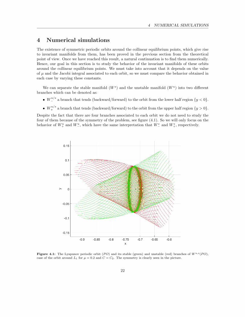
The existence of symmetric periodic orbits around the collinear equilibrium points, which give riseto invariant manifolds from them, has been proved in the previous section from the theoreticalpoint of view. Once we have reached this result, a natural continuation is to find them numerically.Hence, our goal in this section is to study the behavior of the invariant manifolds of these orbitsaround the collinear equilibrium points. We must take into account that it depends on the valueof µ and the Jacobi integral associated to each orbit, so we must compare the behavior obtained ineach case by varying these constants.

We can separate the stable manifold (W s) and the unstable manifold (Wu) into two differentbranches which can be denoted as:

• Wu/s− a branch that tends (backward/forward) to the orbit from the lower half region y < 0.

• Wu/s+ a branch that tends (backward/forward) to the orbit from the upper half region y > 0.

Despite the fact that there are four branches associated to each orbit we do not need to study thefour of them because of the symmetry of the problem, see figure (4.1). So we will only focus on thebehavior of Wu

+ and Wu−, which have the same interpretation that W s

− and W s+, respectively.

Figure 4.1: The Lyapunov periodic orbit (PO) and its stable (green) and unstable (red) branches of Wu,s(PO),case of the orbit around L1 for µ = 0.2 and C = C2. The symmetry is clearly seen in the picture.

22

4.1 Computation procedure 4 NUMERICAL SIMULATIONS

4.1 Computation procedure

In order to avoid numerical problems due to the singularities of the problem, we use three differentsystems of coordinates which have been widely explained in the previous section:

• For points where r1, r2 > ε we use synodical coordinates.

• For points where r1 ≤ ε we use Levi-Civita coordinates around (µ, 0).

• For points where r2 ≤ ε we use Levi-Civita coordinates around (µ− 1, 0).

where ε > 0 is the tolerance chosen (during our study we have used ε = 10−3) and r1 and r2 arethe distances to each primary using synodical coordinates. As it is more intuitive using synodicalcoordinates than Levi-Civita coordinates, we only use Levi-Civita when we are integrating closeto one of the primaries but after having integrated we compute the equivalent points in synodicalcoordinates so all the points are expressed in these coordinates. This procedure is a key part of theproject and must be clearly understood by the reader as it ensures that the whole study remainsaccurate and does not give false behaviors.

Although considering these change of coordinates avoids the singularities of the primaries, a veryimportant issue is to keep the accuracy during the whole integration whichever are the coordinateswe are using, so the best way is to check for every step of the integration if the Jacobi integralremains constant as it is an inherent property of the RTBP from the analytic point of view.

The procedure to compute the periodic orbits around the equilibrium points is nothing morethan a problem of a zero of a function. We are looking for the symmetric orbit with respect to thex-axis in the (x, y) plane around Li with Jacobi integral C, so actually we just need to find halfof the orbit. Due to this symmetry, both the initial and the final points must accomplish x = 0and y = 0, which means that we cut perpendicularly y = 0 at t = 0 and t = T/2, where Tis the period of the symmetric orbit. Using the initial value x0 > xLi

then from the initial point(x0, 0, 0, y0), where y0 = −

√2Ω(x0, 0)− C because of the expression of the Jacobi integral and

the retrograde movement of the orbit, we integrate until we cut y = 0 so we have the point(xf , 0, xf , yf ). Hence, we are looking for a suitable initial value such that xf = 0 when y = 0,which is the perpendicularity condition, so it will provide an initial condition (x0, 0, 0, y0) of thesymmetric periodic orbit.

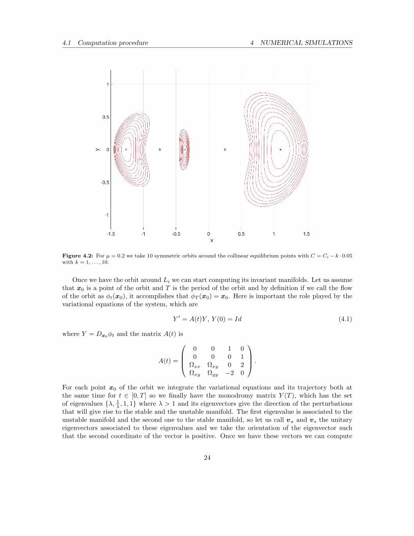
It is very important to find the best approximation of the orbit, so the accuracy must be asprecise as possible because it is the first step of the whole study. To do so, and in order to computethe family of periodic orbits, we start by finding the periodic associated with Ci −∆C, where Ciis the Jacobi integral at the point Li and given ∆C. Once we have the suitable initial condition,we consider a new value Ci − 2∆C and obtain the corresponding initial condition of the associatedperiodic orbit an so on. With this procedure we obtain a family of periodic orbits parametrized byC in a certain range of values C. In figure (4.2), we plot some periodic orbits around Li, i = 1, 2, 3for µ = 0.2 and C = Ci − 0.05k, k = 1, ..., 10.

23

4.1 Computation procedure 4 NUMERICAL SIMULATIONS

Figure 4.2: For µ = 0.2 we take 10 symmetric orbits around the collinear equilibrium points with C = Ci− k · 0.05with k = 1, . . . , 10.

Once we have the orbit around Li we can start computing its invariant manifolds. Let us assumethat x0 is a point of the orbit and T is the period of the orbit and by definition if we call the flowof the orbit as φt(x0), it accomplishes that φT (x0) = x0. Here is important the role played by thevariational equations of the system, which are

Y ′ = A(t)Y , Y (0) = Id (4.1)

where Y = Dx0φt and the matrix A(t) is

A(t) =

0 0 1 00 0 0 1

Ωxx Ωxy 0 2Ωxy Ωyy −2 0

.

For each point x0 of the orbit we integrate the variational equations and its trajectory both atthe same time for t ∈ [0, T ] so we finally have the monodromy matrix Y (T ), which has the setof eigenvalues λ, 1

λ , 1, 1 where λ > 1 and its eigenvectors give the direction of the perturbationsthat will give rise to the stable and the unstable manifold. The first eigenvalue is associated to theunstable manifold and the second one to the stable manifold, so let us call vu and vs the unitaryeigenvectors associated to these eigenvalues and we take the orientation of the eigenvector suchthat the second coordinate of the vector is positive. Once we have these vectors we can compute

24

4.2 Dynamical behavior of the invariant manifolds 4 NUMERICAL SIMULATIONS

the invariant manifolds as follows: from a given point p of the periodic orbit, we take as initialcondition of the associated orbit in the manifold p± s · v where s = 10−6 and v is the eigenvectorchosen depending on the manifold we want to compute and the sign refers to which branch of themanifold we want to study. Hence, in our case we take p + s · vu for Wu

+ and p − s · vu for Wu−.

Although this procedure can be done with any point of the orbit we only choose a finite numberof initial conditions in the linear approximation of the manifold. A posteriori, we check that thisapproximation is good enough for our purpose. We integrate forward in time each initial conditiongiving rise to a trajectory on the corresponding branch Wu. Taking a finite set of initial conditions,we will obtain a finite set of trajectories on Wu.

4.2 Dynamical behavior of the invariant manifolds

In this section it has been described how to find the periodic orbits around the collinear equilibriumpoints from a general point of view so the procedure explained would be valid for any of the threecollinear points. In this project we focus our attention on L1 and consider the range of valuesC ∈ [C2, C1). As we have seen in section 2, the manifolds of the orbit around L1 are enclosed insidethe area defined by the Hill’s region of that level of C, which contains both primaries and L1 butneither it contains L2 (except for the case C = C2 where L2 belongs to the boundary of the region)nor L3, so they will have no effect on the manifolds’ behavior.

Let us fix a value of µ and a value of C. Let us consider the T -periodic orbit around L1 andwe call its initial point when we compute it as x0 = (x0, 0, 0, y0) with x0 > xL1

. Then each point

x0 that belongs to the orbit will be identified with the number θ = tT ∈ [0, 1] where t is the time

needed to reach x0 starting from x0. From now on we will refer to the value θ as the normalizedtime of the point x0.

A very important remark is that we parametrize the set of initial conditions of Wu+ (or Wu

−) byθ in the sense that for each θ we consider the corresponding initial condition of the orbit on Wu asa perturbation perturbation of the point x0, as explained above.

Once we have a periodic orbit around L1, we want to study the behavior of the associatedmanifolds Wu,s. To do so, as we have already said, we will take a finite number of trajectorieson Wu (by symmetry on W s) so we take a finite number of points of the periodic orbit, and thecorresponding suitable initial conditions of the orbits on Wu. We will integrate forward in timeeach orbit until we reach a certain condition.

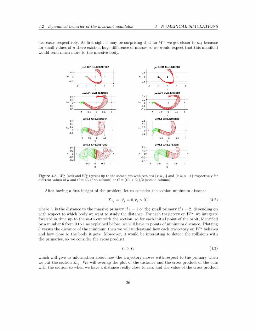
In order to have a first intuition of the dynamics of the invariant manifolds, we compute Wu− and

Wu+ up to the second cut with the sections x = µ and x = µ−1 respectively for different values

of µ and C. In figure (4.3) we plot Wu+ and Wu

− for particular values of µ and two specific values ofthe Jacobi integral C = C2 and C = (C1 + C2)/2 and we notice that for these two levels of C themost remarkable difference is that for the smaller value of C the pipe created by the manifolds iswider than in the greater value case as the periodic orbit describes a bigger trajectory from L1. Onthe other hand, when we vary the mass parameter µ we can see more important changes. When µis small, because of the proximity of the small primary to L1, Wu

+ gets really close to the primarywhile Wu

− stays further from the massive primary. Then, as µ increases the figures show us thatWu

+ gets further but Wu− gets closer, basically because the distance to each primary increases and

25


decreases respectively. At first sight it may be surprising that for Wu− we get closer to m1 because

for small values of µ there exists a huge difference of masses so we would expect that this manifoldwould tend much more to the massive body.

Figure 4.3: Wu− (red) and Wu

+ (green) up to the second cut with sections x = µ and x = µ− 1 respectively fordifferent values of µ and C = C2 (first column) or C = (C1 + C2)/2 (second column).

After having a first insight of the problem, let us consider the section minimum distance

Σri = ri = 0, ri > 0 (4.2)

where ri is the distance to the massive primary if i = 1 or the small primary if i = 2, depending onwith respect to which body we want to study the distance. For each trajectory on Wu, we integrateforward in time up to the m-th cut with the section, so for each initial point of the orbit, identifiedby a number θ from 0 to 1 as explained before, we will have m points of minimum distance. Plottingθ versus the distance of the minimum then we will understand how each trajectory on Wu behavesand how close to the body it gets. Moreover, it would be interesting to detect the collisions withthe primaries, so we consider the cross product

ri × ri (4.3)

which will give us information about how the trajectory moves with respect to the primary whenwe cut the section Σri . We will overlap the plot of the distance and the cross product of the cutswith the section so when we have a distance really close to zero and the value of the cross product

26


cuts the x-axis, at that point there will exist a collision with the primary.

When we use the section Σri we have to take into account that we must distinguish whichbranch we are studying and with respect to which primary, so eventually we have four cases. Oncewe started to compute the intersection with Σri we noticed that we detected minimum distancepoints when the trajectories were still in a neighbourhood of the periodic orbit that caused disconti-nuity issues due to the fact that depending on the initial point of the orbit we detected a minimumnear one of the intersections of the orbit with the x-axis or the other. Hence, we decided to createan initial region where we do not consider the minimum points of a trajectory until it has crossedthe boundary of this region. Let us assume that xmin and xmax the minimum and the maximumvalue of the x-coordinates of the points of the orbit and ymin and ymax the minimum and maximumvalues of y. Then we define ∆x = xmax − xmin and ∆y = ymax − ymin. Then we chose arbitrarilythe initial region as (x, y) ∈ R2 | xmin−α∆x < x < xmax+α∆x, ymin−β∆y < y < ymax+α∆y,where we have generally used α = β = 0.5, although we must adapt these values to each case. Infigure (4.4) we can see an example of the initial region where we have used α = 0.5 and β = 1 forthe case µ = 0.05 and C = C2.

Figure 4.4: Wu− up to the second cut with Σr1 for the case of µ = 0.05 and C = C2. The crosses locate the minimum

distance points of each trajectory. The shaded area is the initial region where we do not gather the minimum distancepoints. In this case we have used α = 0.5 and β = 1.

Once we have all the previous considerations stated we can start to compute the invariantmanifolds, considering the plots up to the first cut with Σri . As Wu

− is pointing to m1, we considerthe first intersection with Σr1 for C = C2 and C = (C1 + C2)/2 for different values of µ.

27


Figure 4.5: First intersection of Wu− with Σr1 . We overlap r1 (red) with the cross product r1 × r1 (blue) for

different values of µ. The first column refers to C = C2 and the second one to C = (C1 + C2)/2.

Figure 4.6: Zoom of the first intersection of Wu− with Σr1 , µ = 0.5 and C = C2. We appreciate collisions with m1

for θ1 ≈ 0.692 and θ2 ≈ 0.907. We plot r1 (red) and the cross product r1 × r1 (blue).

As we see in the figure (4.5), it follows the behavior seen in figure (4.3), where as µ increaseswe get closer to m1. Furthermore, µ = 0.5 is the only value where the difference between the twolevels of C is remarkable because for C = C2 we detect two collisions at normalized time θ1 ≈ 0.692

28


and θ2 ≈ 0.907 as the function r1 × r1 crosses the x-axis and the distance function is numerically0, as it can be seen in figure (4.6).

An important fact that we start to notice in this figure is that for µ = 0.5 there appear jumpdiscontinuities for both levels of C. The discontinuity of C = C2 is produced at normalized timeθ ≈ 0.407 and the discontinuity of C = (C1 + C2)/2 is produced for a small interval of normalizedtime θ ∈ [0.522, 0.526]. These discontinuities will be explained later in this section with more details.

On the other hand we consider Wu+ with respect to m2 using Σr2 . As figure (4.7) shows, there is

not a significant difference on the general behavior of the manifold when varying C apart from thefact that we have collisions for C = C2. We detect four different collisions with m2, two of themfor µ = 0.1 and the other two for µ = 0.5 while for the other value of C we have not detected anycollision for these cases at the first minimum distance.

The main difference obtained has been when varying µ. For the smallest values we see that allthe minimum distance points are quite close to m2 while for greater µ there are points which getfurther from it but other ranges of points get so close that there even exist collisions for the twogreater values studied.

It is also remarkable the discontinuity found for µ = 0.1 and C = C2, which is equivalent to theones of µ = 0.5 and C = (C1 + C2)/2. As before, it will be explained later for another particularcase. In addition, we must notice that the graphics for µ = 0.5 are like the ones obtained for Wu

−but with a translation on the normalized time value of 0.5 (meaning half orbit), which is quiteobvious due to the fact that both primaries have the same mass so their attraction is equal.

Figure 4.7: First intersection of Wu+ with Σr2 . We overlap r2 (green) with the cross product r2 × r2 (blue) for


29


Figure 4.8: Zoom for the first intersection of Wu+ with Σr2 , µ = 0.1 and C = C2. Collisions with m2 for θ1 ≈ 0.333

and θ2 ≈ 0.455. We plot r2 (green) and the cross product r2 × r2 (blue).

In figure (4.8) we see the collisions with m2 for the case µ = 0.1 and C = C2. The collisions ofthe case µ = 0.5 and C = C2 are not plotted because they are equivalent to the ones seen in theother branch of the manifold as we have explained before.

On the other hand, we can consider the second cuts of these manifolds with each section. Aswe can see in the figures (4.9) and (4.10), in the second cut there start to appear important discon-tinuities issues which have to be studied one by one and does not let us study properly the generalbehavior of the manifolds. Also due to these discontinuities, it is quite difficult to interpret thecross product ri×ri overlapped with the distance to the primary, so in these cases we will not plot it.

In figures (4.9) and (4.10), specially in the second one, we see a lot of discontinuities. In partbecause of them, we appreciate that some of the distance values are close to 1 or even greater thanit, so we suspect that maybe these trajectories have escaped to the other primary. When doingthis justification we must take into account the shape of Hill’s region for C = C2 as it can be seenin figure (2.15). Thanks to this property of the RTBP we can claim that if the trajectory is atdistance 1 or greater, it must be close to the other primary.

Except for the case µ = 0.5, the invariant manifold Wu− keeps almost the same distances with

respect to m1 than for the first intersection. Actually for small values of µ this manifold keepsrotating around m1 for much greater number of intersections, which is justified by the more im-portant attraction caused by the massive primary with mass m1 = 1 − µ. On the other hand theinvariant manifold Wu

+ does not behave so well, appearing much more issues than for the otherbranch, justified again by the difference of masses between both primaries which causes that m1

has more attraction than m2.

30


Figure 4.9: Distance of Wu− to m1 at the second cut with Σr1 . The first column refers to C = C2 and the second

one to C = (C1 + C2)/2.

Figure 4.10: Distance of Wu+ to m2 at the second cut with Σr2 . The first column refers to C = C2 and the second

one to C = (C1 + C2)/2.

31


Let us focus on the crossed cases where we consider Wu− with respect to m2 and Wu

+ withrespect to m1. As we are trying to find the minimum distance points with respect to the pri-mary where we are not pointing there appear discontinuities on the first cut with the minimumdistance section as we can find trajectories that initially go to the primary where they are pointingand then tend to the other primary before finding the first minimum distance point while otherreally close points of the orbit start its trajectory and stay near the primary where they are pointing.

Figure 4.11: First intersection of Wu− with Σr2 . We overlap r1 (red) with the cross product r× r (blue) for different

values of µ. The first column refers to C = C2 and the second one to C = (C1 + C2)/2.

Figure 4.12: Zoom for the first intersection of Wu− with Σr2 for µ = 0.5. We overlap r1 (red) with the cross product

r × r (blue) for different values of µ. We appreciate two collisions for C = C2 at normalized time θ1 ≈ 0.451 andθ2 ≈ 0.458. The case C = (C1 + C2)/2 does not show collisions.

As we see in figure (4.11) we do not detect any collision with the primary for the three firstvalues of µ as we are studying Wu

− with respect to m2 but we detect some discontinuities that willbe studied deeper later. Although the first three values of µ does not give us much more informationthan what we already knew, the last one gives us a surprising behavior as for both values of values

32


we detect an interval of values of normalized time such that the branch gets very close to m2 whilethe other ones stay further. In addition we see in figure (4.6) that actually we detect two collisionswith the primary for normalized time θ1 ≈ 0.951 and θ2 ≈ 0.958 for µ = 0.5 and C = C2 while forthe case where C = (C1 + C2)/2 we do not detect any collisions.

Comparing it with the results given by figure (4.9), we see that these same interval of valueswhere we see discontinuities for the first cut of Wu

− with the section Σr2 are the same ones thatgave us discontinuities for the second cut with section Σr1 .

On the other hand, considering the other crossed case where we study Wu+ with respect to m1,

we see again some intervals of discontinuities in figure (4.13) because of the same fact than in theprevious case. In addition we don’t detect any collision for the three first cases but for the last one,because of the symmetry of the case µ = 0.5 between both branches, we can use the same reasoningto justify that there exist two collisions with m1 for C = C2 for θ1 ≈ 0.951 and θ2 ≈ 0.958 and forC = (C1 + C2)/2 we do not detect any collision.

Figure 4.13: First intersection of Wu+ with Σr1 . We overlap r2 (green) with the cross product r × r (blue) for


In the previous figures we have only considered up to the first or the second cut with the sectionbecause for greater number of cuts there were too many discontinuities so we couldn’t do a goodgeneral comparison between the different cases. Although the discontinuities may seem like an errorof the procedure or something bad, they hide a very rich and useful meaning behind them. Afterstudying all the cases we have found three different types of discontinuities:

33


1. Problems with the initial region

2. Homoclinic trajectories

3. Detection of progressive minimums

The first case is basically the one that we can see in figures (4.5) and (4.7) for µ = 0.5 andC = C2. There appears a jump discontinuity because the first minimum points of the trajectoriestend to the boundary of the initial area when varying the initial point associated and then we reachan interval of values which have the first minimum inside the region so we do not detect it eventhough by continuity it exists. Hence, whichever initial region we decided we could not avoid thisdiscontinuity neither for Σr1 nor for Σr2 . As we can see in figure (4.14) where the minimum distancepoints (marked with crosses) tend to the initial region until there is a value where the minimum isinside the region so we do not consider it.

Figure 4.14: Projection on the (x, y) plane of Wu− up to the first cut with Σr1 for µ = 0.5 and C = C2. The crosses

mark when the minimum distance is detected.

Let us focus now on µ = 0.01215, which is the mass parameter of the system Earth-Moon,and C = C2 in order to explain the different discontinuities with a real case which makes it moreinteresting. Although from now on we will study this particular case, this procedure could be donewith other cases because after having done inspections with different values of µ and C, the discon-tinuities found have the same behavior as the ones of the Earth-Moon system, so we will explainthem for this particular one.

As we have seen, the branch Wu− has a very good behavior when µ is small, so for this particular

case we have inspected up to the fourth cross with Σr1 and the behavior seen is quite uniform

34


giving a very well defined shape of the invariant manifold when plotted as we can see in figure(4.15) and without having neither any discontinuity of the distance function nor any collision withthe primaries for the first four intersections.

Figure 4.15: Projection on the (x, y) plane of Wu+ up to the fourth intersection with Σr1 . The crosses mark where

the minimum distance points of each trajectory are produced.

The second type of discontinuities that we have mentioned is the case where there exists a pointbelonging to the orbit such that its associated trajectory ends up again in the initial orbit. Letus consider Wu

− up to the second cut with the section Σr2 . This is one of the crossed minimumdetection which give rise to discontinuities even at the first intersection for certain µ values.

Focusing on Wu+ with respect to m2 and considering up to the second intersection we get the

figure (4.16) plots we can see the second type of discontinuity. Taking a small interval of thenormalized time in a neighbourhood of θ = 0.092 we realize that after the first minimum distancewith m2, which in some cases is quite close as we can notice, some trajectories get close to the initialorbit and some of them go back to m2 but other ones scape to the other primary, but between themby continuity we can assure that there exists a trajectory such that after the first minimum pointwe go back the initial orbit.

35


Figure 4.16: Wu+ first (left) and second (right) intersections with Σr2 . Overlapped r2 (green) and r2 × r2 (blue).

Case of µ = 0.01215 and C = C2.

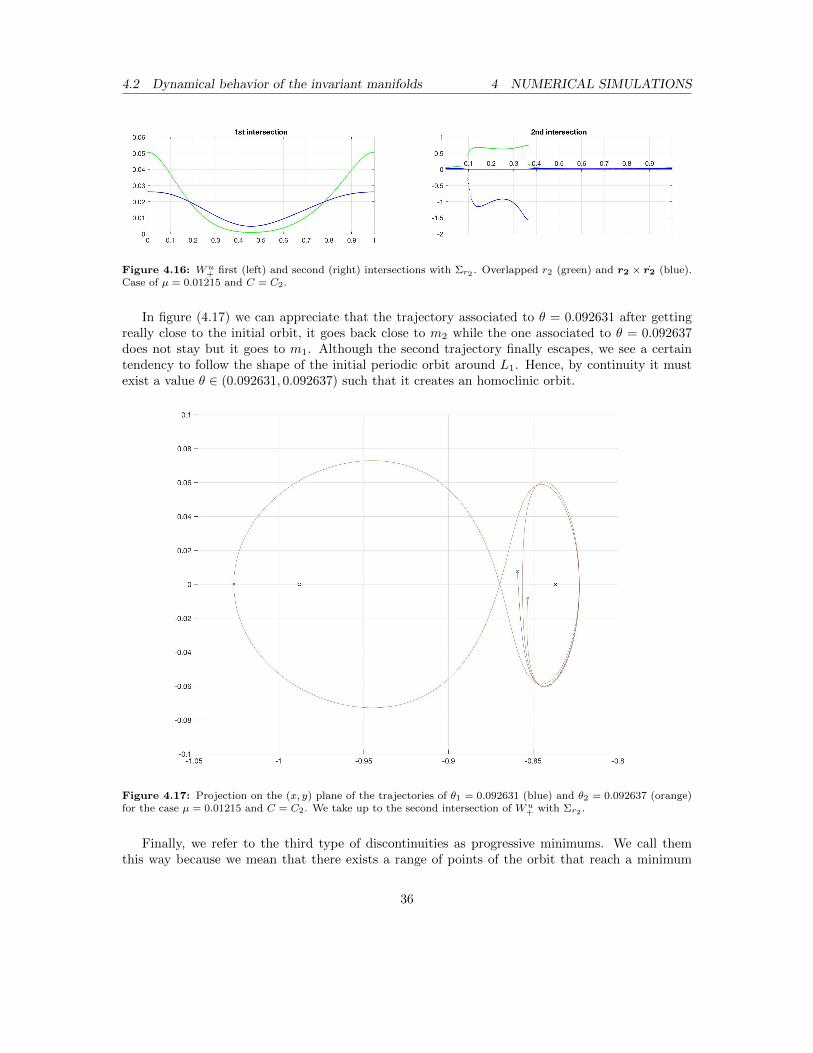
In figure (4.17) we can appreciate that the trajectory associated to θ = 0.092631 after gettingreally close to the initial orbit, it goes back close to m2 while the one associated to θ = 0.092637does not stay but it goes to m1. Although the second trajectory finally escapes, we see a certaintendency to follow the shape of the initial periodic orbit around L1. Hence, by continuity it mustexist a value θ ∈ (0.092631, 0.092637) such that it creates an homoclinic orbit.

Figure 4.17: Projection on the (x, y) plane of the trajectories of θ1 = 0.092631 (blue) and θ2 = 0.092637 (orange)for the case µ = 0.01215 and C = C2. We take up to the second intersection of Wu

+ with Σr2 .

Finally, we refer to the third type of discontinuities as progressive minimums. We call themthis way because we mean that there exists a range of points of the orbit that reach a minimum

36


distance with respect to either of the primaries but other close to this interval does not detect it.These phenomenon creates a jump discontinuity on the graphic of the distance, but plotting thegraphic of the ri against the time for a small group of points belonging to a neighbourhood of theone associated to the discontinuity we can understand why do we detect a minimum only for agroup of points, as we can see in figure (4.20).

Figure 4.18: Wu− first (left) and second (right) intersections with Σr2 . Overlapped r2 (red) and r2 × r2 (blue).

Case of µ = 0.01215 and C = C2.

The discontinuity produced at θ ≈ 0.105 at the right hand side of the figure (4.18) is quiteclear that for smaller values (such as θ = 0.104) we detect the second minimum distance pointmuch sooner than for greater ones (such as θ = 0.106). In order to understand it we can take alook to figure (4.20) where the function r2 associated to θ = 0.104 crosses the x-axis producing aminimum point while the other trajectory clearly does not reach a minimum. We must notice thatthe minimum distance points are produced when we cross the x-axis from the region ri < 0 tori > 0 as in this case we will have ri > 0, otherwise we reach a maximum distance point.

Figure 4.19: Trajectores of the points associated to θ = 0.104 (left) and θ = 0.106 (right) taking the Wu− branch

up to the second cut with section Σr2 . Marked with crosses the minimum distance points to m2.

37


Figure 4.20: Representation of the function r2 with respect with time for the initial points associated to θ = 0.104(blue) and θ = 0.106 (orange) of Wu

− for µ = 0.01215 and C = C2. Complete evaluation up to the second minimumdistance point (left) and zoom of the function at the reason of the discontinuity (right).

This behavior is intrinsic to the manifolds’ dynamics and it is impossible to avoid, so we musttake into account that when studying the RTBP with section Σri there can appear these type ofdiscontinuities. All the other discontinuities of the second intersection of the figure (4.18) are dueto the same fact.

In spite the only way to assure the kind of discontinuity given a plot of the distance to a primaryis to explore it numerically, after having done a lot of inspections we detect a certain tendency thatenable us to distinguish them. If we face discontinuity such that at the edges of the distance functionis quite vertical then we are most probably facing a discontinuity due to an homoclinic trajectory.In this case, if we could take an infinite number of points we wouldn’t find this discontinuity butas we are using numerical methods it is not possible so we see it as a discontinuity. In case that wehave a discontinuity where the edges of the interval change does not create this vertical shape, thenwe will face a case of a progressive minimum or a problem with the initial region. In case that thediscontinuity is found at the first cut then we will need to inspect it numerically to decide but if itis for a greater number of cuts then it will be for sure a progressive minimum point. It is importantto keep in mind that once we have a discontinuity for a certain value θ then all the following cutswith the section will show a discontinuity at that value.

38

5 CONCLUSIONS

5 Conclusions

Despite the fact that this project is mainly numerical, it has been necessary to do a deep studyof the theoretical background related to the RTBP as all the following procedures and results relyon it, specially important has been the research and work devoted to Levi-Civita regularizationbecause they avoid having singularities which would have caused that our study was not reliable atall. On the other hand, once we proved the existence of the periodic orbits and their manifolds wecould start computing them numerically.

The main core of the project has been the one devoted to the numerical study of the problem.We developed a method to compute the orbits around each of the collinear equilibrium points andtheir manfolds, so we could continue this project in the future considering a more general casewhere we could take the orbits around L2 and L3. Our main goal was to describe the dynamicsof Wu,s of the periodic orbits around L1, so we spent a lot of time and energy trying to find thebest way to describe them graphically. We worked with different sections in order to study theinvariant manifolds, such as y = 0, x = µ and x = µ − 1, and after trying to understandall the difficulties and taking into account which of them give us more information we decided thatthe minimum distance was the one that fitted the best with our purpose. The section Σri has thediscontinuities as an inherent property, so we had to adapt to this fact. Thanks to the study of thissection and its discontinuities we have seen collisions with both primaries, homoclinic trajectoriesthat emanate from the orbit and return to it and the progressive minimums, being able to distin-guish between the discontinuities graphically almost for any case.

Once we have studied all the different cases, we have found out that a general study of the case isquite hard to do because when we increase the number of cuts with the section the discontinuitiesalso increase because if a discontinuity appears at the m-th cut, then for all the greater cuts itwill appear too. Hence the analysis of the results are quite complicated to compare between thedifferent values of µ and C used, so this study might be better done case by case studying each ofthem separately so we can discard in each case the discontinuities found and follow the behavior ofthe manifold comparing the results found with Σr1 and Σr2 .

This project has been quite challenging for me, on one hand because of the conceptual difficultyof the project itself but particularly because it meant to me a big change of mind on how to facethis problem. During the degree we are used to working with a clear path to follow when doingan exam, a project or any kind of exercise as we usually follow the guide and tips of the professorwho previously has worked on the case and exactly knows what happens, then more or less weknow what results we can expect. In this project we had a clear goal, but not a clear path, we haveworked on the strategy to reach it, we found unexpected problems which surprised us and we solvedthem by trying other ways to overcome the situation or taking them with a different perspectiveso this issue could become a great result, as it happened with the discontinuities found during ourstudy. Hence, although the Final Degree Project has given to me knowledge and experience dealingwith the RTBP and the manipulation of numerical procedures, I think that the richest part of theproject has been the one related to learn how to organize, to have the capacity of rethinking thestrategy and how to overcome any difficulty appeared during our work. So finally, step by step, weleave the academic way of work and we face the real world.

39

6 REFERENCES

6 References

[1] Barrabes, E., Mondelo, J.M., Olle, M. : Dynamical aspects of multi-round horseshoe-shapedhomoclinic orbits in the RTBP. Celest. Mech. Dyn. Astr. (2009) 105:197–210.

[2] Davis, K.E., Anderson, R.L., Scheeres, D.J., Born, G.H.: The use of invariant manifolds fortransfers between unstable periodic orbits of different energies, Celest. Mech. Dyn. Astr. (2010)107:471–485.

[3] Gomez, G., Mondelo, J.M.: The dynamics around the collinear equilibrium points of the RTBP.

[4] Guckenheimer, J., Holmes, P.J.: Nonlinear oscillations, dynamical systems and bifurcations ofvector fields, Springer Science (1983).

[5] Meyer, K.R., Hall, G.R., Offin, D.: Introduction to Hamiltonian Systems and the N-Body Prob-lem, Springer Science (2009).

[6] Murison, M.A.: On an efficient and accurate method to integrate Restricted Three-Body orbits,The Astronomical Journal, Volume 97, Number 5 (1989).

[7] Stuart, A.M., Humphries, A.R.: Dynamical Systems and Numerical Analysis, Cambridge Uni-versity Press (1998).

[8] Szebehely, V.: Theory of orbits, Academic Press Inc., New York (1967)

40

7 APPENDIX

7 Appendix

For this project, it has been necessary to create programs using Matlab in order to do any necessarycomputation. All the scripts can be found in the following link on GitHub:https://gist.github.com/adriatorrentcanelles/68770a55b2e41884b5f8d9b74c296dc0.

The main scripts are main.m and main plots explicatius.m where most of the computationsillustrated in this project are gathered.

41

title: applications to celestial mechanics author: adrià

Documents