TIMINGIN

TEMPORAL TRACKING

J. A. MICHON

1967

INSTITUTE FOR PERCEPTION RVO-TNO

NATIONAL DEFENCE RESEARCH ORGANIZATION TNO

SOESTERBERG - THE NETHERLANDS

Printed in The Netherlands by Royal VanGorcum Ltd., Assen

PREFACE

A development which has already been in progress for a long time, inindustrial as well as in military work, is that of decrease in the physicalload of tasks to be performed. The recent acceleration in this trendis known as automation.

The decrease in physical load is accompanied by an increase in theimportance of perceptual and fine-manipulatory features of the tasks.The way of measuring perceptual load has therefore become a subjectof great interest.

Michon, who obtained his doctorate with the present study, becameinterested in the timing of behaviour when he considered one of theproposed methods of measuring perceptual load. In that method thedeterioration of performance is evaluated when an additional load,due to a second task, is placed upon the worker. Michon introducedkey-tapping as a second task, and found the irregularity in tappingto be indicative for the level of perceptual motor load. In order tounderstand this phenomenon basically, Michon started this study ontime perception; it deals with very fundamental aspects of humanbehaviour. So in fact a practical question inspired this basic study,which will certainly help to evaluate the key-tapping method asa measure for perceptual load.

A second point that I wish to mention is about the way in whichMichon treats the problem. He completely deviates from the classicalway of studying time perception in that he introduces the method ofsystems analysis which is so frequently used for engineering problemsand, also, in spatial tracking. Although this approach is, of course,the idea of the author, it may be recalled that in the Institute forPerception RVO-TNO people of different disciplines together workon perception problems, under one roof. This set-up has doubtlessenabled an environment in which Michon's ideas could develop fruit-fully.

This approach to the study of time perception will open newways for experimental psychology.

I hope, and expect, that Michon will continue this kind of inventivework on practical problems and basic issues.

PIETER L. W A L R A V E N

CONTENTS

CHAPTER I - I N T R O D U C T I O N 1

1. The problem 12. Mechanisms of time evaluation 33. Non-temporal influences on subjective time evaluation 94. Serial evaluation of time intervals 135. Key tapping as temporal tracking 166. Program of this study 22

CHAPTER II - E X P E R I M E N T A L PROCEDURES 23

1. Some definitions 232. Apparatus and basic procedures 243. Subjects 274. Data collection and reduction 27

CHAPTER III - THE RESPONSE TO STATIONARY INPUT SEQUENCES 29

1. Introduction 292. The isochronic input - Experiment 1 303. Discussion 40

3.1. Synchronization vs. continuation 403.2. Correction of large deviations (Compensation) 413.3. The relation between variability and average interval length. ... 42

CHAPTER IV — THE RESPONSE TO M O D U L A T E D INPUT SEQUENCES. 45

1. Introduction 452. Generating functions and discrete time systems 453. The basic model 494. The simple sinusoidal input — Experiment 2 515. The composite sinusoidal input - Experiment 3 536. The step function input - Experiment 4 567. Two limiting conditions 66

7.1. Selftracking - Experiment 5 667.2. Random modulation of the input sequence - Experiment 6 ... 71

CHAPTER V - QUANTIZATION IN TAPPING 76

1. Introduction 762. The multimodality of tapping interval distributions 77

3. Step-wise adaptation to a modulated input - Experiment 7 814. Conclusions 84

CHAPTER VI — THE INFLUENCE OF N O N - T E M P O R A L I N F O R M A T I O N .

ON TIMING 85

1. Introduction 852. Separate vs. integrated processing of temporal and non-temporal in-

formation - Experiment 8 873. Invariance of the average response — Experiment 9 894. The effect on the response to isochronic input sequences — Experiment 10 915. Conclusions 96

CHAPTER VII - RECAPITULATION AND C O N C L U S I O N S 98

1. Introduction 982. Five features 983. An information processing model of the 'time sense' 101

3.1. Functional structure 1023.2. Decision structure 103

4. Epilogue 108

S U M M A R Y 110

S A M E N V A T T I N G 113

LIST OF SPECIAL SYMBOLS 119

REFERENCES 121

CHAPTER I - INTRODUCTION

1. THE P R O B L E M

This study deals with the temporal aspects of skilled behavior. Wewill investigate the response of human subjects to sensory inputs whichvary in time. Specifically our concern will be the relation between thetemporal structure of an input and that of the associated output.Other properties of the experimental situation will be considered onlyto the extent to which they affect this relation.

With Bartlett (1951), Lashley (1937, 1951), Miller, Galanter andPribram (1960), and others, we are convinced that it is not in the lastplace the fine structure of the timing between successive elements ina string of actions which characterizes skilled performance (Michon1966a).

We might, for instance, study the performance of a pianist playinga Beethoven sonata and measure to what extent his performancewould be in agreement with the specified duration of each note inthe score. Melody and intensity would enter the picture only insofaras they would affect the precision of the temporal relations. A pianistwill be called a 'skilled performer' even by his least benevolent critic,so long as his timing is impeccable, although his 'interpretation' maybe way below an acceptable minimum. In fact there is evidence that'interpretation' is accomplished more by introducing well balancedvariations in the timing of notes than by varying their loudness(Henderson 1936; Stetson and Tuthill 1923).

Rather than trying to cope with the intricacies of Beethoven's pianosonatas, however, we will restrict ourselves to a simpler skill.

In its simplest form the 'timing' of skilled actions can be studiedin key tapping. Here the subject is asked to produce a sequence oftaps by means of a stylus or a Morse key. The sequence may be longor short and it may have a constant or a variable rate. It may be thereproduction (continuation) of an example presented earlier or syn-chronization with a concurrently presented sequence. In the limitingcase just a single interval is involved, a 'sequence' of two taps only,in which case we have the condition which is typical of the classical

time perception experiment. Usually however, the series is longer andthe skill involved is to tap repeatedly as accurately as possible, eithersynchronizing with a stimulus sequence or reproducing such an input.

We intend to single out some of the properties of the mechanismswhich underly the ability to evaluate short time intervals (time per-ception) and which make subjects respond quite appropriately to thetemporal information in sequential stimuli (timing).

In the early days of 'time psychology' no distinction was madebetween time perception and timing in serial behavior. Later, forunknown reasons, it came into existence and consequently the twotopics have developed along quite different lines (Michon 1964b;Weitz and Fair 1951). The notable exception is Fraisse, who didconsiderable amounts of research on both rhythm and time per-ception (e.g. Fraisse 1956,19571). Nevertheless the literature providesno convincing arguments at all for the assumption that evaluation ofa single interval is essentially different from that of a sequence ofintervals. The explanations offered to account for the temporal aspectsof behavior (see Sec. 1.2) are essentially identical for time perceptionand for (anticipatory) timing in key tapping or rhythmic performance.Consequently we will accept key tapping as a valid tool to study themechanisms by which human beings evaluate short intervals of time.

Though rhythmic performance or synchronization are likely torequire more complex processing of information than a 'single interval'experiment, performance under sequential conditions will reveal muchbetter the properties of the time evaluation mechanism. Single intervalexperiments in fact look at the responding system only when it is in atransient state. Hence they deal with a special case and provide onlypartial information about the dynamic characteristics of the timingsystem. On the other hand we should - at least in principle - be ableto derive this special case from more general knowledge about thesystem, obtained by means of a more adequate, i.e. sequential, input.

It is well known that the subjective evaluation of time is highlydependent on factors other than the temporal information from thestimulus condition. The effects of the stimulus and response organi-

1 Fraisse's monograph (1957) has been translated recently. From now on wewill exclusively refer to the English version of 'Psychologie du Temps' : (Fraisse1964).

zation, the intensity of the stimuli as well as their various otherproperties, the amount of information processed and the cognitiveprocesses involved, all markedly influence our estimates of duration,both at a gross level (systematic errors) and in short term fluctuations(variance). We will indicate this complex of factors with the terminformation processing load. It will be analyzed in somewhat greaterdetail in Sec. 1.3, and at a later point we will study its effect on thetiming mechanism (Chapter VI).

In summary then, our objective is to study the timing aspects of asimple form of skilled behavior, i.e. key tapping. Time will thus betreated both as dependent and independent variable, whereas otheraspects of the experimental situation may serve as parameters.

2. MECHANISMS OF TIME EVALUATION

The use of key tapping as a response mode imposes a lower limit onthe range of intervals that can be studied. Bartlett and Bartlett (1959),reviewing the available literature, concluded that subjects cannot tapmuch faster than 10 taps per second, although at the level of muscularinnervation the shortest possible interval is considerably shorter. Theupper limit is in principle determined by practical considerations only.We will, however, restrict the range to intervals of at most 5 sec. Thereis evidence that intervals of more than 3 to 5 sec, are evaluated bydifferent processes than shorter durations (Fraisse 1964; Whitrow1960).

The evaluation of short durations between approximately 50 msecand a few seconds is frequently called 'time perception', an expressionindicating, more than anything else, that neither experimenter norsubject are able to formulate how and to what extent the latter usescognitive or bodily cues. As long as it is not possible to specify theprocesses involved in the estimation of short intervals, we may definetime perception operationally as the ability of a subject to behavedifferentially in response to intervals of various durations, while ex-perimentally noticeable use of cognitive, physiological, or motor cuesis absent. The mechanism of which it is a manifestation will be called,metaphorically, the 'time sense' throughout the text.

The sheer number of hypotheses offered to explain time perceptionhas been characterized as chaotic by more than one author (see for

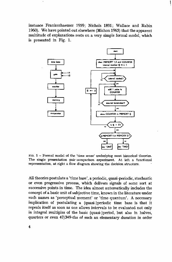
instance Frankenhaeuser 1959; Nichols 1891; Wallace and Rabin1960). We have pointed out elsewhere (Michon 1965) that the apparentmultitude of explanations rests on a very simple formal model, whichis presented in Fig. 1.

dur MEMORY 1,2 and COUNTERinterval number § •«— 1

-11-12

[say -QNE-[ |»y 'TWOJ

FIG. 1 - Formal model of the 'time sense' underlying most historical theories.The single presentation pair comparison experiment. At left a functionalrepresentation, at right a flow diagram showing the decision structure.

All theories postulate a 'time base', a periodic, quasi-periodic, stochasticor even progressive process, which delivers signals of some sort atsuccessive points in time. The idea almost automatically includes theconcept of a basic unit of subjective time, known in the literature undersuch names as 'perceptual moment' or 'time quantum'. A necessaryimplication of postulating a (quasi-) periodic time base is that itrepeals itself as soon as one allows intervals to be evaluated not onlyin integral multiples of the basic (quasi-)period, but also in halves,quarters or even 47/349-ths of such an elementary duration in order

to explain experimental results. The only alternative is to postulatea very short basic interval, e.g. in the order of 0.1 msec as suggested byCreelman (1962).

In the second place the signals generated by the time base have tobe counted during the interval that is to be evaluated. This requiresa gating mechanism, triggered by the 'begin' and 'end' signals of thestimulus intervals, and a counter mechanism or integrator whichaccumulates the time base pulses received during the interval.

Thirdly, it is impossible to present two intervals simultaneously intime evaluation experiments, and in addition an evaluation of thelength of an interval can only be given post hoc. Comparison of inter-vals is therefore necessarily a retrospective comparison of intervalspresented successively. This requires the presence of a memory inwhich the contents of the counter can be temporarily stored.

cl.ar MEMORY and COUNTER

«U 1 pub. laCOUNTER

1

Interval terminated?

do TAP

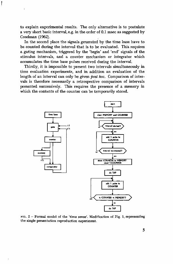
FIG. 2 - Formal model of the 'time sense'. Modification of Fig. 1, representingthe single presentation reproduction experiment.

Finally a comparator or judging mechanism is needed, to comparethe two intervals and to determine the final response.

The diagram on the left in Fig. 1 indicates the functional structureof this model in the form of a block diagram. The situation representedis that of the paired comparison method. The information flow dia-gram at the right shows the logical steps necessary to determine whichof the two successive intervals is the longer.

This model can be modified and made to fit other response methods.In case of the method of reproduction - represented in Fig. 2 - thefirst interval is 'measured' and stored as before. The subject nowprovides his own starting signal for the second interval and continu-ously monitors the difference between the stored duration and theincreasing 'count' of the second interval. When the difference isequal to zero, the 'end' signal is given.

Many processes have been proposed as time basis. Nichols, in 1891,already listed some 50 older hypotheses and Michon (1965) also men-tioned a number of more recent suggestions. A slightly augmentedlist from the latter paper appears in Table 1.

It will be evident from the selection offered in this table, that themajority of the authors attributed the role of time base to very specificprocesses, sometimes observable, like pulse frequency (most recentlyinvestigated by Ochberg, Pollack and Meyer 1964) or respiration cycle(Münsterberg 1889), sometimes purely hypothetical, like James' 'braintraces' (James 1890), fluctuation of attention (Schumann 1893) or'expectancy' (Baker 1962).

None of these theories seems to have great explanatory merit. Theytry to account primarily for the fact that some intervals are estimatedwith greater accuracy than slightly longer or shorter intervals. Mostof the proposed processes - if periodic - have periods around 100 msecor around 700 msec.

The former refer to the possibility, already mentioned, that psycho-logical time is divided into 'perceptual moments' of approximately100 msec. Many perceptual phenomena, such as the perception ofpressure waves in the subauditory range of sound frequency (Stroud1955) or the apparent regularity of temporally irregular visual patterns(Lichtenstein 1961) can be neatly coped with, if one assumes thatpsychological time is discrete in character. The basic idea is thatperceptual information is integrated over a duration of some 50 to

TABLE 1 - Sample of mechanisms and processes proposed as explanatory basisfor the 'time sense'.

Nature of the mechanism Specific process Author(s)

Mach(?) (1865, 1911) >I. Perceptual (immediate)1. 'Time sense' receptors

general sense(analogous to spatial sense) Czermak (1857)

2. Attribute protensity Titchener (1905)Curtis (1916)

II. Cue-theories (mediate)A. External events

B. Internal Events1. Non-nervous physio-

logical

2. Neurcphysiological

3. Psychological

4. Hypothetical

number, rate, differencesbetween events, &c.(overlearning of mentalcontent)

cell-metabolism

metabolism (time of day)heart raterespiration cyclealpha-rhythm

cerebral processescerebellar processes

'pace makers' of the brain(metabolism of brain cells)attentionexpectationbrain trace decay

sensori-motor feedbackcycle

neural scanning

information sampling(perceptual moment)pulse-counting mechanism(signal detection theory)

Guyau (1902)Janet (1928)Frankenhaeuser (1959)Loehlin (1959)Woodrow (1951)

Sunning (1963)

Thor (1962a, b)Ochberg et al. (1964)Münsterberg (1889)Wiener (1948)Latour (1966)Dimond (1964)Braitenberg and Onesto(1960)

Hoagland (1933,1966)Schumann (1893)Baker (1962)Lipps (1883)James (1890)

Adams and Creamer(1962)Pitts and McCulloch(1947)Von Baer (1864), Richet(1898), Stroud (1955)

Creelman (1962)

1 It is highly dubious that Mach may be considered as the major representativeof this view, as Fraisse (1964, p. 80f.) seems to believe.

200 msec, and processed as a single 'sample' (Stroud 1950, 1955;White 1963).

There is no direct physiological evidence in support of this hypoth-esis and it appears that most authors since Wiener (1948) have beensomewhat reluctant to assume that the perceptual moment is directlyrelated to the alpha-rhythm of the brain, which displays periodicitieswith comparable frequencies. In the second place it remains to be seenif the discrete character of psychological time can also be observedwhere the test of the hypothesis matters most: in experiments onsubjective time evaluation.1

The proposed time bases which have their periods clustering aroundapproximately 700 msec, refer to a point on the time scale where thediscrimination threshold for duration is lowest (Fraisse 1964, p. 141f ;Michon 1964b). In the second place this is a point where subjects showneither under- nor overestimation in their evaluation of intervals. Thisso called 'indifference point' was already found in the very first ex-perimental investigation into the domain of subjective time (Höring1864), and since then it has been a source of considerable disagree-ment. In the course of the past century the indifference point hasmoved from a reported 1.5 sec down to approximately 0.7 sec. It hasbeen argued that this might simply be a consequence of the range ofstimuli used, but even though there may be an effect of range or'anchors', this cannot explain the whole phenomenon. Woodrow (1934)showed, by presenting large numbers of subjects with only one singlestimulus interval, that the indifference point is basically range in-dependent (see also Fraisse 1964, p. 119f.).

Even so it remains less than evident, how processes which haveintrinsic periodicities close to the indifference point could serve as'time base', unless we assume with Gooddy (1958) that they combinewith all other periodic and quasi-periodic processes in the organisminto a general 'clock form'. This view - also put forward by Carrel(1931) - may be philosophically valid, but it is hardly a suitable pointof departure for a quantitative analysis of the time sense.

Finally, the results of different authors are frequently contradictory :Schaefer and Gilliland (1938) obtained negative results with respect to

1 Recently a very able review of the 'psychological moment' theory was pre-sented in an unpublished doctoral dissertation by Allport (1966), who stated(Sec. 2 : 2) that "the conclusion that the alpha period does indeed serve as aunit of time in the programming of events in the CNS, leading to a responseseems reasonably well justified".

8

several of the physiological variables listed in Table 1, and there are,for instance, negative findings of Gardner (1935) contrasting withpositive results of Stern (1959) with respect to the effects of metabolism(thyroid function).

The obvious conclusion is that it is premature to attribute the roleof time base to any specific process. More recent investigators, likeCreelman (1962), treat it as a purely hypothetical process. Creelman'soutstanding merit is to have shown that time perception can be treatedpurely quantitatively, without reference to any of the physiological orpsychological suggestions previously mentioned, by using the frame-work of signal detection theory. This model (Creelman 1962 ; reprinted«in Swets 1964) has been described in detail by Michon (1965).

A further important feature of the functional model of Figs 1 and 2,apart from the time base, is the memory store in which the intervalsare stored temporarily. It becomes manifest in an effect which is wellknown in psychophysics : the time-error or time-order error (Wood-worth and Schlosberg 1954, p. 226f.). The first of two successivestimuli in a pair comparison experiment is subject to 'decay', whichaffects the accuracy of the later judgment. With respect to the time-order error in time perception experiments, Frankenhaeuser correctlypointed out (1959, p. 21) that "in respect of subjective time, successionis itself an inherent characteristic of the experience" and hence it is"not an error caused by methodological inadequacies which we want toeliminate, but rather a typical expression of the phenomenon we wantto study".

The time-order error has been observed in two forms. Classically itis found that in the course of time the interval stored decreases inlength (Frankenhaeuser 1959; Woodrow 1951). Creelman (1962) onthe other hand found an increase of the variance as a function of timedelay. The two findings appear to be compatible when interpreted astwo aspects of one particular, imperfect, storage mechanism (See Sec.III.3.3).

3. N O N - T E M P O R A L I N F L U E N C E S

ON S U B J E C T I V E TIME EVALUATION

Psychological time is notoriously inhomogeneous. Accelerations anddecelerations in subjective time experience are frequently a source ofsurprise to everyone, and there is a considerable body of experimental

data about the conditions under which such changes may occur.Fraisse (1964), Loehlin (1959), Orme (1962), and Wallace and Rabin(1960), among other authors, have reviewed many of the relevantstudies.

A first group of factors which is affecting the apparent inhomogeneityof subjective time, without being itself temporal, is organic. Amongthese factors are body temperature (François 1927, 1928; Hoagland1933,1966), time of the day (Thor 1962a, b) and metabolic disturbances(Stern 1959). Noticeable shifts in time perception have also beenreported in experiments with drugs (Frankenhaeuser 1959 ; Goldstone,Boardman and Lhamon 1958; Sterzinger 1938; etc.). Abell (1962),-Goldstone and Goldfarb (1962), Webster et al. (1962), and Weinsteinet al. (1958), for example, reported experiments on the perception ofshort intervals in psychiatric patients.

Although organic factors may exert a considerable influence on theresults of time evaluation, they are likely to remain fairly constantwithin the context of a single experimental session. To the presentstudy they will only contribute part of the error variance.

Related to these factors are the effects due to the structure of thesensory and motor systems. The sensory modality to which thetemporal stimulus is applied is known to affect the accuracy of timeestimation considerably. This is an old finding (see Fraisse 1964, p.104f.), which has been amplified by recent studies, among others byHirsh, Bilger and Deatherage (1956) and Goldstone and Goldfarb(1964). In all studies pertinent to this topic it was found that the earis superior to any other sensory system as a receptacle for duration.Thus it is likely that the properties of the 'time sense' will be obscuredif we use a temporally insensitive input device like the eye. Only ifwe use the ear as an input modality may we be able to establish thelimiting conditions and functional relations of the timing system.

The same argumentation applies with respect to the responsemodality. In the present study we will deal exclusively with intervalsproduced in time, not with their symbolic representation in numbersof seconds as obtained in verbal estimation methods. Although theactual limit on tapping speed is of the order of 10 taps per second(Bartlett and Bartlett 1959), the variations due to the intrinsic 'noise'of the motor system would dominate at rates higher than 3 or 4 tapsper second and drown all variability due to other components of thesystem.

10

The most important factors influencing the inhomogeneity of psycho-logical time, are those related to the specific instructions and taskconditions under which the time evaluation is carried out. The numberof studies in this area is very large; there are reviews by Fraisse (1964),Frankenhaeuser (1959), Loehlin (1959), Orme (1962) and Wallace andRabin (1960), among others. In retrospect this type of research seemsto derive directly or indirectly from an influential essay by the Frenchphilosopher Guyau.

According to Guyau (1902, p. 85f.) "the estimation of duration isrelated : 1) to the intensity of internal images ( .. of stimuli. .) ; 2) tothe extent of the differences between the images; 3) to the number ofimages and their differences; 4) to the rate of succession of theseimages ; 5) to the mutual relations between the images, their intensities,their common properties and their discrepancies, between their variousdurations and temporal interrelations; 6) to the time necessary toconceive these images and their interrelations; 7) to the intensity ofour attention toward those images or to the positive and negativefeelings associated with them; 9) to the needs, desires or affectionswhich accompany the images; 10) to the connections between theimages and our expectations and perspective of the future."1

Although the scientific vocabulary has changed (see Michon 1965,p. 409), it will be evident that Guyau has listed many of the character-istics of what we, nowadays, call 'human information processing', andwe will call this complex of factors accordingly 'information processingload'.

Information processing load encompasses a wider range of conceptsthan was originally subsumed under the heading of 'information theoryin psychology' (Attneave 1959; Garner 1962; Quastler 1955, Van deGeer 1957a, b), which theory after all failed to provide the psycho-logically rich framework it originally promised. Information psycho-logy in this sense is gradually being replaced by formulations in termsof information processing systems, either discursively stated (Broad-bent 1958; Sanders 1967a, b) or formally with explicit reference toinformation processing by computers (Newell and Simon 1963;Reitman 1965).

It is likely that formalization of task factors and instructions, usingthe information processing approach, will solve much of the confusion

1 The eigth item in this list is omitted - probably erroneously - in the 1902edition, which was available to the present author.

11

about the influence of various factors on time evaluation. Michon(1965) gave an example of contradictory findings which probablyresulted from insufficient conceptual clarity, for instance with respectto such ill defined concepts as 'concentrated intellectual work' (Wundt)and 'concentrated attention' (Mach). Wundt (1911, p. 95f.) improperlyequated the two and then drew the wrong conclusion about Mach'smental abilities.

Loehlin's (1959) factor-analytic study has been the most systematicenterprise thus far to determine what factors are responsible for theinhomogeneity of subjective time. He found four factors which wererelated to the specific tasks performed during time evaluation, andinterpreted them as interesting vs. boring, filled vs. empty intervals,activity vs. passivity of the subject and degree of repetitiveness. Loehlin'sgeneral conclusion was that time appears to go 'faster' (i.e. the internaltime base slows down), the more a task constitutes a 'unit' in thesubject's experience. Comparison with Guyau's list reveals a highlevel of coincidence; Loehlin's four factors apparently are majoraspects of the information processing required to perform a task.

Theoretical frameworks providing explanations for the way informationprocessing influences subjective time evaluation are far less numerousthan they are for the psychophysical aspects of time. Frankenhaeusef(1959) is a representative of the cognitive cue theory of time perception.Her hypothesis was that the average number of events experiencedduring an interval is the basis for our judgment of its duration. Infact it is assumed that there is a subjective unit of time, based onoverlearning of an 'average mental content per unit of duration',analogous to the overlearning of the monetary value of coins (Woodrow1951). If there are only few events during an interval, for instance, itwill take relatively much time to reach the critical number of eventsand consequently clock time will seem to pass quickly; this will happenin tasks with high redundancy.

A second point of view is represented by Treisman (1963), whorelated the information processing load to a conceptually differentinternal process derived from the recent discussions about arousal andvigilance: a 'specific arousal process', which determines the pace ofthe time base.

The difference between the approaches seems to be primarily formal.In Treisman's approach inhomogeneity of subjective time is causedby changing a (pseudo-) physiological process, while Frankenhaeuser's

12

hypothesis depends on a judgmental process apparently closely relatedto ideas about short term memory. At the level of specification givenby the authors, however, it is difficult to point out any essential differ-ences between the two hypotheses.

4. SERIAL EVALUATION OF TIME I N T E R V A L S

Thus far our exposition has largely centered around data and theoret-ical considerations that derive from 'single interval' studies. A searchfor original contributions to the theory of time perception from thefield of rhythm has been in vain. (See Weitz and Fair (1951) for abibliography and Fraisse (1956) for a recent experimental study).

Rhythmic skill is attributed to essentially the same kind of processesas time perception. The absence of theoretical distinctiveness doesnot imply that the processes involved are in fact identical. Especiallyin the range below 0.5 sec a different mechanism may be involved inthe evaluation of a single interval than in the evaluation of a sequenceof intervals (Michon 1964b). Fraisse (1956), on empirical grounds,distinguishes between the perception of rhythm (sequences of intervalsunder 500 msec) and the perception of time (over 500 msec).

A second distinction between single and multiple interval experi-ments is found in the direction of the systematic error in time estimates.L. T. Stevens (1886) found that, whilst sequentially produced inter-vals longer than approximately 600 msec are systematically judgedlonger than the standard, intervals under 600 msec are judged system-atically shorter. The reverse is true of the single presentation condition(see Fraisse (1964, p. 116f.) for a review).

Other empirical findings, such as the shape of the differential thresholdcurve and the point of maximum accuracy appear to be comparableunder the two experimental strategies. Although no straightforwardexplanation for the sign-difference of the systematic error offers itself,it might be a consequence of the storage problems which will occurwhen information about successive intervals is stored sequentially.

No systematic suggestions could be found in the literature about thestorage of sequential temporal information. However the presence ofa 'running average' or an accumulating storage, like those found inquality control systems (Page 1954), is suggested by an experiment ofBaker (1962). Baker presented his subjects with a series of irregularintervals with an average duration of 100 sec or 150 sec, and askedthem to produce an interval, subjectively equal to the average of the

13

series. Subjects were fairly well able to do so, but with less precision ifthe stimulus series was made less regular. Furthermore Baker foundthat more recent intervals had a greater influence on the estimatesthan intervals earlier in the sequence. The amount of data and thetechnique used to investigate the serial dependencies do not allowmore quantitative conclusions, however.

This experiment indicates that the analysis of sequential relations isessential to our understanding of the functioning of the serial timingmechanism. Except for Baker's experiment such sequential analysesappear to be absent in the domain of timing and time perception.

When we try to formalize the serial presentation situation in terms ofinformation flow, we see that Fig. 2 can easily be adapted to accountfor the recurrence of taps. In principle the arrangement shown inFig. 3 is the same as that of Fig. 2.

clear MEMORY and COUNTERinterval number § — 1-N

FIG. 3 - Flow diagram for the serial reproduction experiment. Modificationof Fig. 2, to account for repetitive tapping.

Let us consider the situation in which the subject repeatedly repro-duces a standard or sequence of standard intervals given at the outset.The first N intervals are evaluated as standard intervals and stored

14

in memory in some weighed combination. The first subject-producedtap will coincide with the last signal of the standard. From that firsttap on, the subject will compare the memory contents with the intervalin progress. When the difference between stored and actual intervalequals zero, the memory is updated, a tap is given and a new cyclestarts. Crucial to this arrangement are again the properties of thetime base providing pulses to the counter, the way the memory doesor does not combine old and new information, and the rate at whichthe memory contents decay. Experimental data will have to providethese parameters.

In the case of a synchronization experiment, in which the subjectaims at coincidence of his taps with an external train of signals, theflow diagram becomes more complicated since the task requires moni-toring of the external input. Several alternative models suggestthemselves, but to present these at this point would be premature.We return to them at a later point when we shall summarize ourempirical findings (Chapter VII). In how far the 'internal standard'of the reproduction experiment is functionally equivalent to the'external standard' in the synchronization condition also remains tobe seen.

We expect the concomitant aspects of the experimental situation - theinformation processing load - to exert an influence on the timeevaluation processes involved in key tapping as much as they do inconventional time perception experiments. This idea has been workedout in some detail by the present author in studies on the measurementof information processing load or perceptual (-motor) load (Michon1964a, 1966a, b). In these investigations the regularity of key tappingduring the execution of a second task was used as an indicator of theload imposed on the subject by that task. The index of regularity wasfound to vary predictably with some of the quantifiable aspects of thesecond task.

Not much is known as yet about the way in which sequential timingis affected by non-temporal information. A thorough investigationwould lead us too far beyond our present endeavor of providing aformal framework for the description of timing behavior, but we willdeal with the interaction between temporal and non-temporal in-formation in a few exploratory experiments in Chapter VI.

15

5. KEY TAPPING AS T E M P O R A L T R A C K I N G

Key tapping is in several respects comparable to manual tracking ofa visual input ; we may call it temporal tracking. It consists either ofsynchronizing with a time-varying input, which is analogous to pursuittracking, or of keeping a sequence of taps as regular as possible, whichmay be looked at as a form of compensatory tracking, i.e. the subjecttries to maintain his tapping rate at a previously set (internal) stand-ard. Spatial tracking has been studied very extensively: Adams(1964), Ellson (1959), Licklider (1960) and Bekey (1962), in that order,offer reviews of increasing technical complexity.

An approach frequently adopted in the analysis of spatial trackingbehavior is derived from electrical engineering, and is known as'systems analysis'.1 It is quite distinct from the classical approach tosensori-motor performance in that it takes into account the sequentialrelations that exist between an output and current, as well as previous,states of an input, and does so in a mathematically rigorous way.

In essence the technique, as it is employed in tracking studies, is tosubject a 'black box' - a system of unknown composition - to a speci-fied input and to describe the output of the system as a function of theinput, taking into account all phase, frequency and amplitude relations.The analysis can be carried out either in the frequency domain interms of sine wave responses, or in the time domain in terms of, forinstance, step or pulse responses. In the first case the response of asystem to a sinusoidal input is studied. The analysis is based on thepossibility of describing any function of time by a weighed linearcombination of simple sine waves (Fourier synthesis). Hence theresponse to an input function can be calculated if the responses tothe simple functions y = sin cat, for 0 ^ a> 5g oo, are known.

If the analysis is carried out in the time domain, the system is, forinstance, subjected to a step function

) T <? 0't -* ^s U It 1 \

and the way in which the system adapts itself to this sudden disturb-ance is studied.

1 Much of what follows is based on: Licklider (1960), Ragazzini and Franklin(1958), Schwarz and Friedland (1965) and Truxal (1955).

16

The necessary assumption, made in both approaches, is that thesystem is linear. A linear system is characterized by the 'superpositionprinciple' which states that the response to an arbitrary combinationof inputs is equal to the combination of the responses to each inputseparately, or

Hfi (T) + H/a (T) + . . . + Hfn (T) == H {A (T) + f z (T) + ... +fn (T)} (1.2)

in which Hft(T) stands for the response to the input function fi(T).(See Schwarz and Friedland 1965, p. 12.) The function relating theoutput of the system at any moment to the input to which it is, andhas been, subjected is called the 'transfer function', though it is not afunction in the mathematical sense, but a complicated operator on theinput function.

The transfer function is essentially a functional mathematical de-scription of the system hidden in the black box. As such we are ableto predict from it, what the response of the system will be to any giveninput function. Its main advantage is the fact that it takes intoaccount the time-varying aspects of the input, i.e. its history. Themajor drawbacks of the transfer function as a model are, in the firstplace, that it is a very general model - the same transfer function canbe derived for an infinity of actually realizable systems, whence it isvoid of psychological content - and in the second place that it hingeson the linearity assumption. The 'superposition' principle is veryimportant because of its mathematical convenience, but is is onlyapproximatively valid when we are dealing with living systems.Considering Eq. (1.2) in the light of absolute thresholds, forexample, will make it obvious that such thresholds must reflect certainnon-linear properties of the system, since they imply that some changesin the input signal will have no corresponding effect in the output.Usually biological systems contain other non-linear components aswell, and usually these are difficult to cope with.

There are at least two ways of reducing these problems. First, onecan stretch the linearity assumptions somewhat and deal with thesystem as quasi-linear, in which case all non-linearities are pooled andtreated as 'noise' together with genuine noise generators in the system(Licklider 1960, p. 177f.). A second alternative is suggested by thework on human information processing models (Newell and Simon

17

1963; Reitman 1965). Many of the non-linear effects in humanbehavior, such as thresholds, can be treated as all-or-none or binarydecision processes. Such either-or relations are difficult to incorporateinto an ordinary transfer function, but can easily be accounted for ininformation processing models. Apart from this advantage the in-formation processing approach allows us to circumvent the mathe-matical complexities of non-linear systems analysis, without anysacrifice in rigor. Finally it enables us to impart psychological contenton a model more easily than can the vocabulary of systems engineers.

In this study we will approach key tapping as the temporal analogueof spatial tracking and treat it accordingly. The reason why we haveadopted the systems approach rather than the customary regressionanalysis to account for serial effects is that we feel that the determin-istic character of the transfer function with its stable parameters, isconceptually closer to the information processing approach than arestochastic models.

In conclusion of this section, key tapping studies which bear at leastsome relevance to the foregoing will be reviewed.

Accuracy of tapping has been determined by several authors. Thefirst to employ sequential tapping was L. T. Stevens (1886), whostudied tapping in the range between 0.27 and 2.9 sec. His subjectswere required to synchronize with the clicks of a metronome and tocontinue tapping at the same rate after the metronome was halted.Stevens concluded that long intervals are progressively made longerand short intervals progressively shorter, with an 'indifference point'between 0.53 and 0.87 sec, depending on the subject. The longer thestandard interval, the greater the overestimation, which may be ashigh as 10%. In reverse the same applies to short intervals.

The second finding of Stevens was that subjects tend to alternatelonger and shorter intervals. This was taken as evidence for theexistence of a correlation between successive intervals, due to a com-pensating mechanism. However, the argument is invalid since thealternation was observed relative to the previous interval and notrelative to the average interval length.

Later investigators have essentially confirmed Stevens' results, andalso specified the accuracy of performance (relative error) at differentrates, which Stevens had left out of consideration. Because of trends,sometimes present in sequential tapping, some authors have not onlyused the variance as a measure of dispersion, but also the summed

18

first differences between successive intervals (Fraisse 1956; Michon1964a, 1966a, b). Irrespective of the measure used, it is found thataccuracy passes through a maximum between 500 and 800 msec,decreasing to both sides (Bartlett and Bartlett 1959; Davis 1962;Fraisse 1956). This implies that Weber's law does not hold for time,but there is no common quantitative opinion as to what extent it doesnot hold (but see Treisman 1963). In terms of system properties itsuggests that there may be an intrinsic periodicity in the organismwhich becomes tuned to the input interval when the two are approxi-mately equal in length.

The same is suggested by the phenomenon of 'personal rate'. Ifsubjects are allowed to tap at a rate which they prefer subjectively,all settle down at a rate which is not too far from the point of leastvariability mentioned above. Miles (1937), in a sample of almost 200subjects, found that 80% spontaneously chose intervals between 200and 700 msec and only 11% preferred intervals of more than 1 sec.Later authors have confirmed this. The personal rate has been used todemonstrate the influence of other factors on sequential time evalu-ation. Denner et al. (1963,1964) showed that the personal rate changedafter the subject had been exposed to temporal information presentedat rates different from the preferred tempo. In our own, previouslycited studies of the variability of the personal rate as a function ofinformation processing load, irregularity was found to increase withload. No consistent changes in the personal rate itself were foundthough, which may indicate that only the variability is affected by theinformation processing load of a task and not the period length of themechanism of which personal rate is the manifestation.

Data about the way sequentially produced intervals are distributedare very incomplete. Bartlett and Bartlett (1959) reported that thedistributions of intervals longer than 1 second are normal, but those ofvery short intervals approach rectangularity, because the noise of themotor system starts playing a predominant role. Lichtenstein andWhite (1964) reported approximately normal distributions for inter-vals of 500 msec, and Ehrlich (1958) found the same for intervals of600 msec. These findings might be indicative of a true gaussian noisebeing responsible for the variability in the results, but this conclusionis not warranted without additional evidence.

The adequate input to a dynamic system is a time-varying input aswas pointed out earlier. Key tapping in response to such an input has

19

been studied in the first place in experiments on rhythm. Herevariations in interval length are usually very frequent. The number ofintervals in a sequence is characteristically of the order of three to six,runs of equally long intervals usually being not longer than two orthree. Hence we are likely to measure performance while the systemis in a transient state. Secondly the rhythm is mostly reproducedafter the stimulus has been presented - which requires a memory forseveral intervals at once. Synchronization, although very importantin musical ensemble performance, has not been studied at all.Notwithstanding these restrictions we may make a few qualitativeobservations from such studies as Seashore's (1926) or Fraisse's(1956).

When short intervals are followed by one or two longer intervals,we observe an overshoot in the reproduced group, in at least the firstlong interval after the shift. An overshoot in the other direction maybe observed if the transition is from long to short (Fraisse 1956, ch.4,5). These findings suggest that there is an effect of preceding inter-vals on later performance, in other words: a dynamic relation. Thesize of the overshoot decreases in some cases when the shift becomessmaller, just as we would expect if the overshoot were relative to thesize of the shift.

Three more studies should be mentioned. Gottsdanker (1954),comparing manual and temporal tracking, had subjects extrapolate(continue) quadratically accelerated and decelerated series. From hisresults it can be inferred that in both conditions subjects laggedbehind the expected value extrapolated from the previously producedintervals. Since his was a continuation experiment, the results maynot be directly comparable in terms of lags and leads in synchroni-zation performance, but they are suggestive of a comparable dynamicresponse to internal as well as external standards.

Ehrlich (1957, 1958) compared continuation and synchronization inkey tapping. Although he also did not apply any sequential statistics,his experiments are close to our endeavor and deserve a more extensivereference.

In one study Ehrlich (1957) compared tapping at the personal rate(average interval length of 6 subjects: 605 msec) and synchronizationwith a 600 msec standard sequence. The results showed that foursubjects had less variable results when performing at their own ratethan when they were synchronizing. This was taken as evidence forthe thesis that spontaneous tapping is at least as regular as synchroniz-

20

ing and that the responsible 'neuro-motor' mechanism is not regulatedor 'driven' by the external input.

In a more comprehensive study Ehrlich (1958) dealt in some detailwith this problem. Subjects were asked to synchronize with an iso-chronic (600 msec) sequence, or with linearly accelerating or deceler-ating series with rates of change of ± 10, 20, 50, 80 or 100 msec perinterval and ranging between 300 and 2000 msec. In addition 'cyclic'sequences were given with alternatingly positive and negative acceler-ation, and a random sequence of intervals, also ranging between 300and 2000 msec. Ten subjects were used altogether. The results of thisstudy may be summarized in the following points.

There were only very minor systematic errors, i.e. lags or leads withrespect to the input sequence. Deviations from the accurate intervallength were said to be normally distributed, but no quantitativeanalysis was provided.

The higher the rate of change, the larger the standard deviationsof the results. This was taken as evidence by Ehrlich that the timingmechanism can only cope with stationary stimuli, and breaks downwhen the input is variable. Compensatory behavior (phase regulation)was said to be absent or at least very inadequate : the stimuli seemedto play no decisive role in maintaining the regularity of key tapping,but no analysis to illustrate this conclusion was provided.

Ehrlich's final conclusions deserve to be quoted in full (1958, p. 21) :"Thus the decreased regularity of the accelerated and deceleratedsequences should be nothing but the observable expression of a gradu-ally failing mechanism, which normally is restricted to regulatinguniform, repetitive actions". And he added (p. 22) : "It seems to bedifficult to go any further with our description. At this point thepsychologist has to give the floor to the neuro-physiologist."

The present study will prove that the psychologist can in fact go agreat deal further, without committing himself once again prematurelyto any of the neuro-mythological mechanisms that have blossomed soabundantly in time psychology.

There remain a few remarks to be made on a recent study of Fraisse(1966), who investigated the adaptation of tapping immediately afterthe onset of the input sequence. He found that the correct rate isestablished after about three intervals, which implies an 'overshoot'like we have noticed before, and that little systematic error remainsin a subject's performance. He showed in addition that the same istrue, when the rate of the input sequence is suddenly doubled or halved,

21

an experimental condition which is related to the 'step function input'used in the present study.

The interpretation given by Fraisse is, like that of other authors inthe field, completely qualitative and offers no conceptual frameworkfor a quantitative framework to describe data.

6. PROGRAM OF THIS STUDY

We are now in a position to formulate the program of this study. Wehave found that many of the findings on key tapping have been derivedfrom preciously few data. Moreover, even investigations that werebased on more extensive data do not report any comprehensivestatistical analysis. In two respects all studies on key tapping that wereferred to in the preceding sections are deficient. First, they containno data on the distribution of intervals; most only give means andstandard deviations, few indicate qualitatively the shape of thedistributions. Secondly, no sequential statistics have been computed,although we found that it is likely that each tapped interval dependsto some extent on preceding intervals.

It is exactly these two aspects of the data, that will have to provideus with the information we need about the type of dynamic mechanismthat is responsible for timing in key tapping. The main objective ofChapters III and IV is to provide such data, for the case of stationaryand modulated inputs respectively. We will derive from these datasome formal properties of a 'time sense' conceived of as a dynamicsystem.

In Chapter V some of the collected data will be reconsidered in thelight of the hypothesis that psychological time is discrete in character.

In Chapter VI we shall deal with the influence of information pro-cessing load on the formal properties of the timing mechanism. Thischapter specifically reports three exploratory experiments on the im-pact of a well defined component of information processing load, eventuncertainty, on timing behavior.

Chapter VII finally, offers a recapitulation and a synthesis of theexperimental results of the earlier chapters. In particular we willplace the results in the formal framework of the information processingmodels treated in the sections 2 and 4 of the present chapter.

First however, a technical prologue to the experimental chaptersthat follow will be given in Chapter II.

22

CHAPTER II - EXPERIMENTAL PROCEDURES

1. SOME D E F I N I T I O N S

In some experimental conditions subjects have been presented withauditory stimulation consisting of sequences of clicks, and were re-quired to tap in synchrony with these clicks. This condition will becalled synchronization in contrast to continuation, where no concurrentclick sequence is presented and the subject tries to extrapolate a seriesof auditory intervals presented earlier.

In the second place we distinguish between stationary, or isochronic,and modulated sequences. In the first case the intervals of the stimulussequence and - ideally at least - the intervals of the response sequenceare all of exactly the same duration. This type of input is comparableto the 'direct current (D.C.) level' in an electrical system: a constantvoltage applied to the input of the system.

Modulation of the input and studying the response to it, is the maintechnique for testing dynamic systems (Sec. 1.5). In the presentcontext modulated sequences consist of intervals which are not allof the same length. A sequence may be called random, for example,if the durations of successive intervals are independent of one another.The intervals may be constant up to a point and then suddenly changeto a different but equally constant value ; this type of modulation canbe called a step function. Several types of modulation will be used inthis study; examples are shown in Fig. 4.

A special way of representing intervals which will be used systemat-ically throughout this monograph is shown at the top of Fig. 4. Insteadof indicating intervals as marks on a time line, the length of the intervalis plotted as a value on the ordinate of a Duration/Order diagram.Along the abscissa successive intervals are equidistant and labeled bytheir rank order number in the sequence. Using this representation weavoid some of the problems which we would encounter if we undertookto draw Duration/Duration diagrams of our experimental results.

In order to distinguish between the various aspects of time consideredin this study, a number of special symbols will be used as fixed con-ventions. They are defined in the 'List of Special Symbols' at the end

23

T,

t

t'i-

t

T

rA t

«b.*

(a)

t

t.

At

,1*ba«:

(c)

t

tt-« -

W

Ti TI T, T« T,

t,

i<2 ;s j* «s' s / /

' frf1 2 3 4 5 > • i

t

t

" ""A r; \ AI

IT" ib».

- 4 - 2 0 2 4 »• i (b)pulse

t

.-_- t

-A -ne

-if

i\7— 'b«.:

2 0 2 4 f i ( d )galive step

*st\' *-

T„

ê

'l|

- 4 - 2 0 2 4 »positive step

' . i

" ?"l If

-Vf Ivf0 2 4 0 »•

triangular

;:tÉ-( e ) 0 2 4 - - - O

sine wavei (f) O 2 - - -

random

FIG. 4 - Graphical representation of stimulus and response sequences.Top : linear and two-dimensional (Duration/Order) representation of intervals ;a-f: some input functions.

of this monograph (page 119). Other symbols used in the text conformto statistical and mathematical conventions or will be defined wherenecessary.

2. APPARATUS AND BASIC PROCEDURES

The basic equipment used in the experiments is depicted in the dia-gram of Fig. 5. Most of the components of this setup were developedin the Institute for Perception RVO-TNO. It consists in essence of a

24

very precise stimulus timing set and an equally precise response timingand recording set. Since in some experiments the two parts interactedthey are shown together in one figure.

FIG. 5 - Block diagram of experimental apparatus.

During an experiment the subject was seated in an isolated room,with all the necessary stimulus presentation and response productionequipment, but no timing and recording apparatus, in order to ruleout temporal cues from the sounds of relays, punched tape readers,etc. The illumination level in this room was kept at a comfortablelevel. Outside noise could not always be avoided entirely but was tosome extent attenuated by the earphones the subjects were wearing.

The subjects produced intervals in one of two ways. In experimentswhere no controlled variation of information processing load wasinvolved they tapped a delicately adjusted Morse key, with a springload of approximately 50 grams. If on the other hand they wererequired to respond differentially to a set of stimuli (from 2 to 8alternatives), they pressed the appropriate response keys of a set of

25

eight. The spring load of these keys was not identical for all fingers,but all fell within a range between 25 and 35 grams. An essential partof the instruction was to make the subject respond abruptly, and teachhim to avoid pendular movements of fingers or arm.

In each of the two methods the response intervals were measured inmilliseconds by means of a digital counter (Hewlett and Packard 521D)which after each response was automatically reset and started. Theintervals measured were printed on paper tape by means of a Hewlettand Packard 561B printer. The values printed were exactly 200 msecless than the actually produced intervals, because of the print-reset-start latency. This arrangement restricted the possible range of inter-vals at a lower limit of 200 msec, which was not serious since the lowerbound imposed by the intrinsic noise of the human motor system is ofthe order of 300 msec. Intervals below that value have not beenstudied.

When differential responding was required, both the stimuli present-ed (selected by means of punched tape reader II) and the responsesgiven by the subject were printed along with the response time, thusallowing an error analysis.

The apparatus used in the synchronization experiments was triggeredby another punched tape reader (I) which read the sequence of encodedinterval durations. These were fed into a digital preset counter, oper-ating in milliseconds, which could be given any preset value betweenzero - in which case it produced exactly the encoded sequence - and10 sec, which then was added to the encoded values. A binary dividercould furthermore change the internal clock speed of the preset counterby factors of 2,4, 8 or 16. By means of this provision the average inter-val length could for instance be doubled without changing the ratiosbetween the intervals in the sequence, while using only one piece ofsingle punched tape. The output of the preset counter was finallyshaped into square pulses, amplified and fed into a headphone inthe subject's room. The clicks presented to the subjects were keptthroughout at a level of 45 db above threshold.

In some of the earlier experiments the intervals were not generatedby means of the digital counter just described, but by means of aHewlett and Packard 202A low frequency oscillator. This undoubtedlyintroduced slight variations in the length of the input intervals.However, fluctuations were found to stay well within the tolerancelimits specified by the manufacturer, and hence will not have deviatedmore than 0.5% from the average. Moreover such fluctuations were

26

always very slow in comparison to the average interval length.Consequently they will have manifested themselves as trends in thedata, rather than as noise-like short term fluctuations.

In one experiment (Exp. 5) subjects had to synchronize with theirown delayed output sequence of taps. The output, i.e. the last tapproduced, was fed through a discrete step delay line, and subsequentlyback to the earphones. The delay was variable in 60 steps of equallength, since the line essentially consisted of 60 flip-flop circuitswhich were triggered one after another at regular intervals. In ad-dition the length of the steps could be varied by means of an externalclock, a variable pulse generator.

3. SUBJECTS

Six subjects (B, M, N, S, vdV and vD) took part in the experiments ona regular basis. They were full time employees of the Institute forPerception RVO-TNO. Experiments in which other subjects wereused, are specified as such. All six regular subjects, five male and onefemale and aged from 20 to 30 years, were highly trained during earlierexperiments not reported in this study, pilot experiments and specialtraining sessions. All had normal hearing, except for N, who showeda slight impairment of one ear between 5 and 10 db with respect to thethreshold for clicks. No special correction needed to be made for this.

Because all subjects were in some way involved in the project,they may be considered to have had adequate motivation to sit throughthe sometimes quite strenuous experimental sessions.

4. DATA COLLECTION AND R E D U C T I O N

The amount of data collected in a single experimental session - nosession was longer than 30 min - varied considerably as a function ofthe average interval length. On the average about 500 intervals werecollected per session, usually in runs of 100 or 200. No data havebeen left out of consideration except when contaminated by technicalfailures. The first 10 or 15 intervals of a run, though, were systematic-ally discarded, because we wanted to exclude initial effects from ouranalysis.

Uninterrupted runs never lasted more than 10 minutes.If a subject complained of fatigue or loss of concentration, or if he

27

showed marked deviations from his ordinary level of performance, thesession was adjourned.

The large amount of data obtained (approximately 500,000 intervals)made it necessary to use computer facilities. Yet, much of the datahave been reduced by sheer manpower. Specifically most of themore complicated, time consuming, calculations such as serial corre-lation, spectral analysis, trend elimination and tests of goodness of fit,have been executed with a digital computer.

28

CHAPTER IIITHE RESPONSE TO STATIONARY INPUT SEQUENCES

1. I N T R O D U C T I O N

An isochronic sequence of intervals may be looked at as if it were a'direct current (D.C.) level'. If we apply a constant voltage c to alinear electrical circuit, the output will also be a constant voltage,though not necessarily equal to the input. The response to a time-varying input, when superimposed on a D.C.-level, will not alter itscharacteristics since

H (i(T) + c} = Hf(T) + c', (3.1)

in accordance with the superposition principle (Sec. 1.5). A variableresponse to a constant input on the other hand, is indicative of spon-taneous activity of the system. Such activity may consist purely of'true' noise, but may also result from non-linear properties of thesystem. An analysis of the response to stationary inputs is therefore anecessary prelude to the study of modulated inputs.

We may, in principle, expect several types of spontaneous activityin the 'time sense'. In the first place there can be the non-stationarityor drift of the system parameters, which occurs in most living systems.Under its influence the tapping response will be affected even whenthe instruction is that the subject keep his tapping rate as constantas possible. Fortunately such trends are usually slow in comparisonto the tapping intervals and thus can be accounted for quite easily.

In the second place we may expect to find considerable interval-to-interval variation : time evaluation experiments are notorious for theirlarge variances. Before we attribute such short term fluctuations torandom processes in the organism, we shall have to determine if thereare any sequential relations, periodic or a-periodic, hidden in the ap-parent 'noise' produced by the subject. Such relations can be extractedfrom the noise by means of autocorrelation techniques. If no serialrelations are indicated by the (linear) autocorrelation function, wewill assume that there is a stochastic process without memory under-

29

lying the variations in performance. From the characteristics of theinterval distributions we may then proceed to infer what type ofstochastic mechanism is involved (McGill 1963; Restle 1961).

Related to the foregoing is a third non-linear effect which may showin the data : quantization of psychological time will reveal itself in theresponse distributions as multimodality since, if there is such a thingas a 'time quantum' T, a response interval will ideally consist of anintegral multiple of T.

A further point must be given attention to in this chapter, namelythe difference between synchronization and continuation, the latterbeing treated as tapping 'in synchrony' with an internal standard.The feedback of temporal information is likely to be more complicatedin the former situation, since the subject may extract additional in-formation from the time difference between a click and the corre-sponding tap, but it is not yet clear how far this possibility is anadvantage to the subject in the case of isochronic input sequences.Ehrlich (1957) found for instance that synchronization does not showless variability than continuation at the personal rate, as we saw inSec. 1.5. Analytically the presence of any compensatory mechanismwhich makes use of this extra information must reveal itself in theautocorrelation function of an output sequence 'as being dependenton at least some of the preceding intervals.

Finally we shall have an opportunity to look into the problem of theapplicability of Weber's law to time perception, which has beenquestioned for more than a century (Fraisse 1964 ; Mach 1865 ; Michon1964b; Nichols 1891; Treisman 1963).

2. THE I S O C H R O N I C I N P U T - E X P E R I M E N T 1

Procedure

Four subjects from the regular pool of six - S, vD, M and N - producedtwo series of 200 intervals at each of 6 standard durations: 333, 500,667, 1000, 1667 and 3333 msec, both in the synchronization and thecontinuation mode; 96 series in all.

The apparatus was described in Sec. 11.2.In a pilot experiment, of which some results will be mentioned, three

subjects each produced two series of 200 intervals at each of 10standard durations: 333, 400, 590, 667, 833, 1250,1667, 2500 and 3333

30

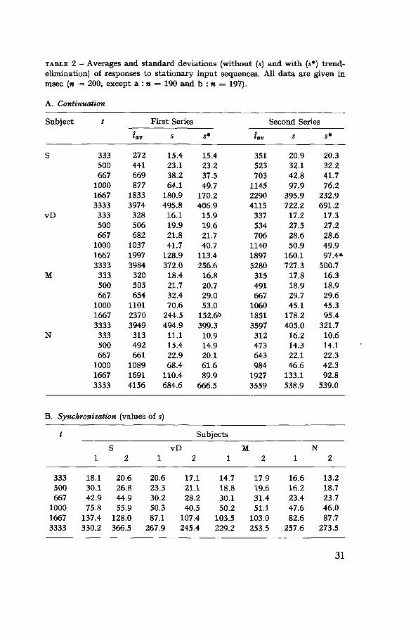
TABLE 2 - Averages and standard deviations (without (s) and with (5*) trend-elimination) of responses to stationary input sequences. All data are given inmsec (n = 200, except a : n = 190 and b : n = 197).

A. Continuation

Subject

S

vD

M

N

t

333500667

100016673333333500667

100016673333333500667

100016673333333500667

100016673333

B. Synchronization

t

333500667

10001667

S1

18.130.142.975.8

*av

272441669877

18333974328506682

103719973984

320505654

110123703949313492661

108916914156

(values

2

20.626.844.955.9

137.4 128.0

First Series

s

15.423.138.264.1

180.9495.8

16.119.921.841.7

128.9372.018.421.732.470.6

244.5494.9

11.115.422.968.4

110.4684.6

of s)

vD

Second Series

s*

15.423.237.549.7

170.2406.9

15.919.621.740.7

113.4256.6

16.820.729.053.0

152.611

399.310.914.920.161.689.9

666.5

Subjects

1 2 1

20.6 17.23.3 21.30.2 28.50.3 40.87.1 107.

,1 14.7.1 18.8,2 30.1,5 50.24 103.5

tav

351523703

114522904115

337534706

114018975280315491667

106018513597312473643984

19273559

M2

17.919.631.451.1

103.0

s

20.932.142.897.9

395.9722.217.227.528.650.9

160.1727.3

17.818.929.745.1

178.2405.0

16.214.322.146.6

133.1538.9

1

16.616.223.447.682.6

s*

20.332.241.776.2

232.9691.2

17.327.228.649.997.4»

500.716.318.929.645.395.4

321.710.614.122.342.392.8

539.0

N2

13.218.723.746.0ST. 7

3333 330.2 366.5 267.9 245.4 229.2 253.5 257.6 273.5

31

msec. The stimuli in this pilot study were generated with the low-frequency oscillator (see page 26). Not all cells of this design werefilled however, and data were collected in a less detailed form than inthe main experiment.

Results

Non-stationarity. Slow spontaneous variations in tapping rate weredetermined by fitting to each of the 96 series a polynomial

ti = a0 + aj + a#* + . . . + a*f* (3.2)

in which ti is the duration of the i-ih interval (see the List of SpecialSymbols, p. 119). The method of least squares (Lewis 1963) was usedto find the best fitting polynomial and the maximum degree resultingin a significant reduction in the amount of residual variance.

For the synchronization series no consequential improvement result-ed from the trend elimination, quite unlike the continuation sequencesfor which polynomials of degrees up to 7 were found to reduce thevariance of the results considerably. This can be inferred by comparingthe columns s (raw standard deviation) and s* (standard deviationafter trend elimination) in Table 2A.

Fig. 6 shows the trends of the continuation sequences graphicallyon a logarithmic scale. Two points deserve to be mentioned withrespect to this diagram. First, the range of the trends becomes largerwith t, both in an absolute and a relative sense. This points to arelatively small efficiency of storing the internal standard - or aconsiderable decay factor - when the intervals are long. In the secondplace the trends do not follow a consistent pattern although we finda systematic error in the average (4» — t'^0), away from the indif-ference point at approximately 700 msec (see Table 2A: îav). This isin agreement with L. T. Stevens' historical data, both qualitativelyand quantitatively (Stevens 1886).

The conclusion - also to be drawn from Fig. 6 - is that the majorshift in 4» takes place during the very first 10 or 15 intervals afterthe discontinuation of the standard sequence, which were not takeninto account in the present analysis though.

All subsequent analyses of the data have been carried out on trendeliminated data (residuals).

32

V.O.eooor

2500AOOOr

1000

1600

700L1000

450L700

350L

500

200L

3333

1667

1000

»&.- 667

500

•'- 333

100 200

FIG. 6 - Trends, eliminated from the raw data of the continuation sequences ofExp. 1. The vertical time scale (msec) is logarithmic.

Short term variations. The correlation between an interval 4 and itspredecessors ^_i, 4-2, ... is expressed in the autocorrelation function

R(k) = '-=1m

(3.3)

33

in which m = n — k,

0.5(3.4)

while s* is identical to so except that the summation is not overI ^i ^m but over k + l ^ i 5Ï «. 4»i and 4»2 are the averages ofthe first m intervals and the last m intervals respectively. This functionis essentially Pearson's product-moment correlation coefficient, calcu-lated over m pairs of values of $ }, for different lags k ^ O.1

We have calculated R(k) for lags O ̂ k ^ 15 for 8 continuation and8 synchronization series, randomly chosen from the set of 96. Thisnumber was judged to be sufficient since the function R(k) was fairlyinvariant over subjects and values of t, although it was evident thattrend elimination had not always been complete in the 1667 and 3333msec series. The average R(k) functions of the continuation and thesynchronization series are shown in Fig. 7.

i.o

0.5

-0.5

R(k)

contin. synchr.

10 15 0 10 15

FIG. 7 - Autocorrelation functions (average of eight) of continuation and syn-chronization sequences. Vertical bars indicate standard deviations.

Since R (k) has to exceed ± 0.181 to be significant at the 1% level,under the assumption that it is allowed to consider separate values ofR(k) for different k as independent for a first approximation,2 it may

1 An extensive treatment of continuous and discrete autocorrelation functionscan be found in Blackmail and Tukey (1959).2 In fact R(k) should be evaluated integrally and not for individual values of k.A good test should take into account the overall variations in R(K). No simpletests are available however, and moreover they would in all likelihood not havealtered our conclusions.

34

be concluded from Fig. 7 that there is in both experimental conditionshardly any serial dependency, even with respect to the immediatelypreceding intervals (i.e. for k = 1, 2). Yet it seems possible to dis-tinguish between the two presentation modes. It can be seen in Fig. 7that in the synchronization condition 4 tends to be negatively corre-lated with îi-i, and perhaps slightly with 4-2, whereas there is a traceof positive correlation in the continuation series. A Student t-test forthe difference between the averages of -R(l), R(2) and jR(3) under thetwo response modes gave t = 9.63, 4.17 and 0.37 respectively, the firsttwo values of t being significant at the 1% level, with 7 degrees offreedom.

Our conclusion is that there is a distinction between the two modes.The trend towards positive serial correlation in the continuation modemay be the result of an incomplete trend elimination, since the functionR(k) seems to approach 0 only very gradually. It may however, justas well be the manifestation of a more fundamental distinction betweenthe two conditions. This may be clarified by later parts of our analysis.

The synchronization condition shows a, perhaps minor, but demon-strable effect of negative feedback (compensation), which proves thatat least some of the extra information provided in this situation isused to maintain the synchrony between input clicks and output taps.

Grosso modo, however, we can agree with Ehrlich's (1957) contentionthat a synchronization error in tapping is not systematically compen-sated for. In fact it is, but only very little, and for a first approximationwe may perhaps leave the effect out of consideration.

Analysis of extreme deviations. Before we adopt this strategy, we haveto consider the possibility that the effect of compensation is presentbut buried in the variations due to other noise factors in the system.It was suspected on the basis of some early unpublished observationsthat there is a compensatory mechanism to deal with extreme devi-ations (of random origin) from a regular tapping rate. Since suchextreme deviations are rare, the mechanism would operate only in-frequently, whence the effect on the autocorrelation function R(k) issuppressed when it is determined for the response sequence as a whole.

The data on which this observation was based are of course suspect,since our analysis consisted of looking at the records and samplingsome convincing instances. Nevertheless, the effect may be real: itmight indicate that there is a threshold below which errors in regularityare not - or not noticeably - compensated for.

35

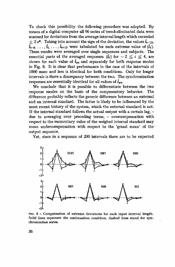
To check this possibility the following procedure was adopted. Bymeans of a digital computer all 96 series of trend-eliminated data werescanned for deviations from the average interval length which exceeded± 2 s*. Taking into account the sign of the deviation, the values 4-io,4-9, . . . ,îi, . • • , 4+10 were tabulated for each extreme value of {4}.These results were averaged over single sequences and subjects. Theessential parts of the averaged responses {4} for — 2 5ï i ^ 4, areshown for each value of îav and separately for both response modesin Fig. 8. It is clear that performance in the case of the intervals of1000 msec and less is identical for both conditions. Only for longerintervals is there a discrepancy between the two. The synchronizationresponses are essentially identical for all values of îav.

We conclude that it is possible to differentiate between the tworesponse modes on the basis of the compensatory behavior. Thedifference probably reflects the generic difference between an externaland an internal standard. The latter is likely to be influenced by themost recent history of the system, which the external standard is not.If the internal standard follows the actual output with a certain lag, -due to averaging over preceding terms, - overcompensation withrespect to the momentary value of the weighed internal standard maymean undercompensation with respect to the 'grand mean' of theoutput sequence.

Yet, since in a sequence of 200 intervals there are to be expected

1000

3

2

1

O

-1

-2

3

2

1

O

-1

-2i

FIG. 8 - Compensation of extreme deviations for each input interval length.Solid lines represent the continuation condition, dashed lines stand for syn-chronization series.

333

36

only about 10 extreme deviations which exceed ± 2s*, and since theeffect of compensation does not extend beyond the first two intervalsfollowing the extreme, there is no immediate reason to doubt that mostfluctuations from one interval to another can be treated as seriallyindependent. We shall have to determine more precisely however,what the threshold of the compensatory mechanism implies, and howit operates (see Sec. III.3 and Chapter IV).

The relation between variability and interval length. The relation be-tween the variability and the average length of the response intervalhas been plotted in Fig. 9, for each of the four subjects. Except at thelower end of the range of lav, where s* (or, by definition the differentialthreshold at = s*) seems to approach an asymptote, the results can beexpressed by an exponential relation :

ÔÎ = kt™ + a, (3.5)

where A is a constant of the order of 0.040 and a may be visualized asthe intrinsic noise level of the motor system. The slopes of the leastsquares linear regression lines fitted to the data plotted in Fig. 9 donot deviate significantly from the lines with slopes 1.5 actually drawn.

Once more the results of the two presentation modes appear to beidentical, which is further confirmed by some results of the pilot ex-periments, of subjects M and N, which have also been plotted in Fig. 9.The exponent being larger than 1, the relation between ôî and lav

cannot be explained in terms of a simple stochastic process ; a suggestionfor a more complex mechanism will be made in the discussion (Sec.III.3.3).

Distributions of interval durations. The type of stochastic processresponsible for the variations in interval length reflects itself in thedistributions of intervals. Some of these distributions are shown inFig. 10. Each class interval of the distributions shown was 5 msec, anda smoothing procedure has been applied to suppress some irregularity,such that

0.5 #i_2 + #j_i + xi + *i+i + 0.5x i = ------ — - -

All distributions of t — 1667 and 3333 msec, and some of 1000 msecshow quite pronounced multiple peaks, suggesting very strongly that

37

1.0

0.5 -

0.2

0.1

0.05

0.02

1.0

0.5

0.2

0.1

0.05

0.02

0.01

: ' 1 l l l l l I 1 1 h-t-; :

M.

61 = 0.0 501 i, A /' -•

V.D.

6Î= 0.044l'-5

I I I I I 11 i—i—i-

et =0.050 "t

0.2 0.5 5 0.2 0.5

FIG. 9 - Variability of the response to isochronic input sequences as a functionof the average length of the output intervals. Time in sec.

Continuation 1st series: + 2nd series: •

Synchronization 1st series : » 2nd series: o

Pilot Study 1st series: A 2nd series: *

response intervals are quantized, an important fact, which will betreated in detail in Chapter V. The absence of multimodality in thedistributions of shorter intervals can be caused by the intervals fallingwithin the range of a single 'peak'.or time 'quantum'.

38

333msec

1667msec

FIG. 10 - Examples of responseinterval distributions. The dash-ed curves are normal distri-butions fitted to the actualdistribution. N.B. The very thintails of the distributions arerecording artefacts.

3333msec

In order to suppress the multimodality shown in Fig. 10 and tobring out the gross shape of the distributions, further smoothing wasachieved by increasing the width of the class intervals to a point whereunimodality was obtained, the average number of classes being about25. The distributions then were compared with a normal distributionby means of a #2-test (Lewis 1963, p. 227f.). The probability levelsassociated with the %2-values range from very high to very low andhave been plotted in Fig. 11. The two distributions of ̂ -levels deviatesignificantly from the expected distribution as is shown by the %2-valuesin Fig. 11.

90 99 100V.

FIG. 11 - Distribution of ^»-values associated with the x2-test for normality ofinterval distributions, (a) continuation; (b) synchronization. Dashed linesrepresent the expected distributions of ^»-values.

39

A closer inspection of the exceptions did not reveal any commonfeature. Hence we will consider them as irregularities in the generalpattern and treat the distributions for our present purposes as resultingfrom a normal - or binomial - random process.

3. DISCUSSION

3.1. Synchronization vs. Continuation

In retrospect we may conclude that there are observable differencesbetween the two presentation modes in at least two respects. In thefirst place there are trends in the continuation sequences which mayeasily extend over a range of 20% of the average interval length. Wehave found no particular pattern in the course of these trends, but itis evident that most of the displacement with respect to the standardinterval length occurs very early in a series and may be consideredas a transient effect. The second difference found between continuationand synchronization performance was in the compensation of extremedeviations (exceeding ± 2s*) at long intervals. When the intervals wereshorter than some value between 1667 and 1000 msec, no distinctioncould be made again.

It seems plausible that both effects are the result of special featuresof the 'internal standard' which the subject maintains in the continu-ation condition. Unlike the external standard, the internal standardwill follow the fluctuations in the output sequence to some extent -albeit with a certain delay and in a smoothed fashion. This can ac-count for the observed discrepancy, as we have argued before (p. 36).On the basis of the present data we are not in a position to analyze theproperties of the internal standard in a quantitative way. The data- such as were shown in Fig. 10, for instance - make it plausible how-ever, that the 'running average' which is the internal standard, isbased on a few preceding intervals only, e.g. a number between 3 and 7.

There is some evidence (Ehrlich 1958) that subjects from time totime lose external control in the synchronization condition and ap-parently 'track' an internal standard for a few intervals until thesynchronization error becomes too large, or perhaps until some otherdecision intervenes. In a later chapter (Chapter V) we shall be in abetter position to evaluate such loss of external control, when weshall generate synchronization errors externally.

40

3.2. Correction of large deviations (Compensation)

Compensation of discrepancies between the standard - both externaland internal - and the actual response seemingly occurs only if aparticular 'tolerance level' is exceeded. This situation is in the firstplace reminiscent of dynamic quality control systems in industry(Page 1954). Changes in machine operations, to maintain a certainstandard of quality are usually very costly, and have to be kept to aminimum. Products are therefore allowed to vary freely within certainlimits and corrective action is taken only when these limits are ex-ceeded. The decision rules may be based on a variety of statisticssuch as fixed or weighed averages, and numerous strategies are em-ployed to bring quality back to standard. A psychological theory ofthe perceptual moment based on these techniques was developed byShallice (1964).

A plausible alternative for the 'quality control' paradigm is theassumption that the compensatory mechanism depends only on theabsolute size of the error e< = £< — tt, which itself is of course a functionof tav. If the error is smaller than a threshold value below which itcannot be detected or below which it is not possible to perceive thedirection of the error (Hirsh and Sherrick 1961), no action will be taken,but for the rest the compensation will be entirely a function of e onlyand not of lav. Since ôî is directly associated with îav the consequenceis that the compensation of small errors which are easily detectable,will have no noticeable effect on the output sequence $ } or its variousstatistical properties.

Assume, for example, that tav = 1 sec and that ôî at 1 sec is equalto 50 msec. Then an error et at instant i, which is of the order ofmagnitude of 0.5 öl and which is compensated for 80% at instant * + 1,would change the value of ôî from 0.050 to 0.054 when averaged overa number of observations. This would be a difference which is noteasy to detect in experimental data. An error ej = 1.5 ôî, on the otherhand would have the effect of changing ôî from 0.050 to 0.078.

This alternative seems to be more attractive than the quality controlmechanism, since it explicitly recognizes the phenomenological distinc-tion between the duration of the intervals of a sequence and the ex-perience of a time difference between tap and click, the synchronizationerror.

We are, of course, interested in compensation effects that are ob-servable, and in the way in which such compensation is effectuated.Both points can be studied more appropriately if the deviations are

41

introduced by the experimenter rather than by chance. Only then canwe determine the dynamic properties of the compensatory mechanismquantitatively. This will be undertaken in Chapter IV.

We may conclude this part of the discussion by stating that, aslong as the discrepancy between input click and output tap is relativelysmall, the compensation effect is drowned in fluctuations which canbe treated by a fair approximation as originating from a stochasticallyindependent gaussian source.

3.3. The relation between variability and average interval length

If we disregard deviations exceeding the 'tolerance limit' and - atleast for the time being - the apparent quantization effect observedin the interval distributions, the probability density function <p(l) ofthe response intervals may be described simply by the normal densityfunction,

yfl=-J-exp (V ' s V2rc 1

(3.7)v '

being the probability of an interval having exactly length î. Sinces ~ s* = dî = kî^, in the range ôî ̂ 0.5 sec, we have

_ - eXp - - • • (3-8)

kî%V2n \ 2k* II I ^

Expression (3.8) is nothing but a convenient summary of a large partof the results of Exp. 1.

As was said earlier, there is no simple stochastic process in whichthe variance increases at a rate greater than that of the mean, and wehave to think of a more complex mechanism to account for the 1.5power relation between ôî and iav. The exponential relation in factsuggests, according to Zwislocki (1965), a kind of self -regulating mech-anism, of which the sensitivity decreases as a function of the sizeor intensity of the stimulus. Such mechanisms are difficult to visualizepsychologically. The following essay to account for the results shouldtherefore be considered as very tentative.

The relation expressed in Eq. (3.5) derives from the inevitability ofthe time order error in experiments on time evaluation (Sec. 1.2). Wehave argued that one interval must be stored in memory whilst and

42

as long as the next interval is in progress. We shall assume that thisinterval estimate is subject to decay while it is stored, i.e. during theperiod of storage the interval may increase or decrease in lengthrandomly. It has a constant probability p+ of increasing one basicunit of time, a probability ^>_ of decreasing one unit and a probabilitypo = (l — p + — p-) of remaining unchanged. The length of the storedinterval (ts) will on the average, stay constant over time if p+ = p_and in general Ave (t s) = t s + n(p+ —p-), while Var (t s) = n {(p+ +p-) — (p+ — p_)* }, in which n is the number of points in time, since t&was stored, at which an event (either -f, — or 0) occurred.

Because in general, in the tapping situation, n oc t s, it will be evidentthat the variability bl of the tapping sequence {4 } will be proportionalto the square root of Var(fo) and consequently dl <x \/n oc \/lav.

If this mechanism is also 'self-regulating' in the sense describedabove, we have to make the additional assumption that the size ofthe unit steps up and down is a function of the sensitivity of thesystem, rather than a constant. Specifically, if the step size is directlyproportional to îav, we will have the multiplicative relation di =A!*>.6. k2î = *M, where k = k^.k2.

In psychological terms this means that, after all, Weber's law wouldhold for time (Treisman 1963; Fraisse 1964, p. 141f.; Michon 1964b),were it not for the decay in time of the stored interval. One questionwhich remains unanswered is, how Treisman (1963) and some otherauthors managed to avoid the decay of the memory component. Ingeneral we do find however, that results of threshold experimentsreported in the literature are in fair agreement with the 1.5 exponentialrelation found in the present experiment (see Michon 1964b, Fig. 1;Woodrow 1932).

Three final remarks should be made. First, the assumptions madeabout the behavior of the stored interval requires the variance to beproportional to time-since-storage. This has been substantiated notonly for time intervals, but for other stimulus dimensions as well (seeCreelman 1962).

In the second place the proposed mechanism - however provisional -renders the position of a (quasi-)deterministic 'time quantum' lessabsolute : if an interval were estimated by counting successive quanta,the decay of the stored count would not be in units of constant sizebut at its best in integral multiples of such units, proportional to îav.

Thirdly, only if p+ = p_, will the average length of stored durationsremain constant. If p+ < p-, for instance, the average will become

43

smaller, or behaviorally, tapping becomes faster while the variancewill change accordingly. The parameters p+ and p- may conceivablyplay a role in situations where information processing load is imposedon the subject. The information processing channel can be lookedat as a 'single channel transmitter' which can deal with only onesource of information at a time and alternates between differentsources (Broadbent 1958; Egeth 1967; Welford 1967). It seems plau-sible that the probabilities of losing or gaining units of the storedinterval t s will be affected by the amount of non-temporal informationimposed on the subject.

Although we will return to the problem of information processingload in Chapter V, we will not work out the foregoing speculativesuggestions, since we will deal primarily with synchronization sequen-ces. In that case the relation p+ = p- is automatically guaranteedby external means, i.e. the input sequence.

44

CHAPTER IVTHE RESPONSE TO MODULATED INPUT SEQUENCES

1. I N T R O D U C T I O N

The present chapter is devoted to the problem of what determinesthe length of the 'next' interval produced by the subject in thecourse of synchronizing with a modulated input function. What earlierinformation is stored in 'temporal memory' and how are errors insynchronization, that are well above threshold, compensated for?Such very large errors do not occur spontaneously in normal tappingperformance and have to be introduced externally by changing therate of the input clicks, i.e. by modulating the input sequence.Continuation experiments are not feasible in this setting: the subjectwho has to change the rate of his internal standard in a prescribedmanner, will act as a final rather than a causal system, which leads toproblems beyond the scope of this study.

In the answer to the question posed in the last paragraph the dynam-ic properties of the timing system - or metaphorically: the 'timesense' - will become manifest. A dynamic analysis requires somemathematical manipulations of a kind that is not yet widely usedin psychology. The following introduction to the technique of systemsanalysis by means of generating functions may contribute to make thispowerful technique better known. The arguments and symbolism usedin the next section are focussed on our present enterprise, but are basedlargely on the following texts, which offer more general and morerefined expositions: Ragazzini and Franklin (1958), Schwarz andFriedland (1965) and Truxal (1955). Feller (1957) offers an illuminatingchapter on generating functions.

2. G E N E R A T I N G F U N C T I O N S AND DISCRETE TIME SYSTEMS

We deal - in abstracto - with two series of numbers which representsequences of input intervals and output intervals respectively.We are interested in the relation between these two series, andwant to include the possibility that not simply £< = ƒ(<«), but that

45

îi = 1(ti, tt-i, . . ., ^i_fc). Moreover we want to generalize this ex-pression and find a relation between input and output sequence,{4} = H {t{}, which is independent of the particular value of ». In thelatter representation H is an operator - called the 'system transferfunction' - which generates the output sequence $ } if {$< } is input to it.Generating functions and specifically the ^-transformation (related tothe Laplace transformation) may be used to achieve these goals.

A generating function is an expression for the sum of an infinitepower series, and it will generate that series upon expansion in aunique way. It is an engineering convention to use an expansion innegative powers of a dummy variable z. Thus the sum F(z) defined by

F(Z) = 2 /w«-1i-0

is called the z-transform of the function /(t).1 For example, if F (z) =zl(z — 1), expansion by long division generates the series 1 + z-1 -4-z-2 + . . . + z~k + • • • , whence by Eq. (4.1) the original function isfound to be f(i) = 1, for all i^ 0. Here and later it is always assumedthat ti = 0 for i < 0.

Conversely we may determine the ^-transform of the function

/W = (*)':

(4.2)2z —

Again by introducing the dummy variable z, we are able to regeneratethe terms of the original series {1, 1/2, 1/4, 1/8, . . .} as coefficients ofthe power series of which F(z) is the sum.

The 2-transform makes the derivation of the transfer function of adynamic system in principle very easy. In Fig. 12 the response to asimple pulse input tg at » = 0 is represented in the upper section of thefigure. The response is shown as extending over the next few instantsi = 1, . . . . 4 and returns to zero for i > 4. The response function canbe expressed as {tghg, tghi, . . . M»*}- In the type of linear systemswe are studying, the height of the input pulse (tg), appears only as amultiplication constant in the response function. Hence we can sayin general that the sequence {hg, h\, ... hu} = {hi} (where it is assum-

1 i is exclusively used to indicate the rank order (instant) of intervals, not todesignate y^l.

46

ed that A« = 0, for t' 3; k) is the transfer function we want to know.It fully determines the response of a linear system to any given inputfunction. For, if the system is given a second pulse input t\ at i = 1,the response to *i will interfere with that to the pulse given at * = 0,and later input terms will add their contributions and combine into acompound response function. The essence of the 'composition' or'convolution' of successive terms is depicted in Fig. 12.

t,h,

•c £J" -? .?II N II

-ws

FIG. 12 - The principle of calculating a convolution sum.

47

Under the linearity assumptions all contributions simply add, andthe general response term can therefore be expressed as

(4.3)fc-O

Now the use of the «-transformation in the present context will be-come clear: it relieves us from the need to carry out, step by step,the summation of Eq. (4.3) for each value of i separately. Instead wemultiply the ^-transforms of the input {£<} and transfer functions {hi},to obtain the z-transform of the response function {^ }, i.e.

f(z) = T(z).H(z], (4.4)

or, if input and output sequences are known and the transfer functionis to be determined, we obtain by algebraic division :

(4.4a)

The relations expressed in Eqs (4.4) and (4.4a) follow directly from themultiplication or division. Since

T(z) = h

and

H(z) = h0

we have

T(z).H(z) = f(z) =

£ '*A<-* ) ^ + • • •*-0 /

as required by Eq. (4.3) with respect to the response terms.Once {hi} or H(z) are known $} can be directly predicted for any

given input sequence {ti} at any point in time.

Although we have dealt with the sequences of intervals completelyabstractly, we may consider them, more concretely, as input and outputof a psychological system, the 'time sense'. A representation of the'time sense' which to us is a black box of unknown composition, isgiven in Fig. 13a.

48

(a) (b)

HM

t« .H».TM

FIG. 13 - 'Black box' representation of dynamic system, without and withexplicit feedback loop.

Since subjects are predicting the length of intervals on the basis ofprevious information, the black box must contain a feedback loop.Hence we may replace it by the diagram Fig. 13b, which is the basiclayout of a system with negative, i.e. error correcting, feedback. Theresulting error function transform E(z) which is the ^-transform of thedifference between the transforms of input and output, passes througha 'reduced' black box, with transform G(z), which describes the responsefunction when the feedback loop is interrupted (open loop transferfunction).

In Fig. 13b the various relations between the ^-transforms are indi-cated. Since E(z) = T(z) — f(z) and f (z) = E(z).G(z), we can derivethe relation between the transforms of the general transfer function,H (z), and the open loop transfer function G(z) :

3. THE BASIC MODEL

The model proposed is extremely simple but can be refined andaugmented easily with the technique introduced in the previoussection. It rests on three basic assumptions.(a) If the input sequence is isochronic, the subject will synchronizeperfectly - disregarding the noise component in his performance -after the first two intervals, i.e. if {tt} = C for i ^ 0, then £< = £< forall i ^ 2.

This applies to the ideal case only. In our data we have tried toapproximate this ideal by averaging out random variations in theresponses.(b) Memory for previous input intervals is restricted to a perfect

49

memory for the immediately preceding interval £j_i. In the absenceof further information, therefore, I = t^\.(c) If at any instant i we change the rate of an isochronic input to adifferent but also constant rate, an error will occur (see Fig. 14).We assume that the error en — i{_i — £j_i is compensated for im-mediately and completely at the next interval, such that îi = ^_i +BI_I. Consequently ̂ = t^\ + (*t-i — 4-i)- Since sub (b) we assumedthat li = ti_i if the sequence is isochronic, we have

(**-i - «(-2) = 2*i_i - tt-t (4.6)

as a general expression for the i-th response interval as predicted bythe model. The relation expressed in Eq. (4.6) also describes the per-formance of the model when more complicated changes in inputoccur: irrespective of {£$} the predicted value ̂ is a linear extrapolationfrom the last two input intervals t^i and 2j_2-

Since Eq. (4.6) only describes the local behavior of the system atinstant i, where t 2ï O, we have to derive the general expression forthe relation between input and output sequences. Starting from Eq.(4.6) we find that the input function {*,} = {1, 1, 1, £, — £, . . .}has as response {1} = {0, 2, 1, 1, 0, — 1|, . . .}, as is shown by way ofan example in Fig. 14. By our earlier arguments we arrive at

T(Z\ l -f- 2-1 + 2-2 + l?"3 + . . . 22

for the transform of the model's closed loop transfer function, whilethe open loop transfer function is described by the transform

\ / -i IT/.A /„ i \o* V /

which follows directly from rearranging Eq. (4.5) and substitution ofEq. (4.7).i

H(z) and G(z) characterize the properties (a), (b), and (c). Theexperiments described in the remaining part of this chapter weredesigned to test this model, which may be called an 'ideal linearpredictor'.1 A mathematically more elegant way of deriving the transfer function is tocarry out directly the ^-transformation of the difference equation describing thesystem (Eq. 4.6). This results in the expression Eq. (4.7).

50

• stepwidth

-2

- 2 0 2 4 6

FIG. 14 - Graphical representation of the response (solid curve) of an ideallinear predictor to an input function (circles). Extrapolation of the differencebetween successive circles yields predicted values (crosses) of next outputinterval.

4. THE SIMPLE SINUSOIDAL I N P U T - E X P E R I M E N T 2

The input sequence tested in this experiment is defined by

2mtt = thai + At sin —, (i ̂ 0).

16(4.9)

The input varies between tbas and t bas + At, while one period, D,consists of 16 intervals.

Design.

Three subjects, vdV, B and vD each produced 10 complete periodswith tbas = 600 msec and with tt>as = 1200 msec, while At = 0.32 tbas-

Results and discussion.

The average response of subject vdV to both input sequences is shownin Fig. 15, in which the vertical scale for t^as = 1200 msec is half aslarge as that of the other condition to make the two parts of the figuredirectly comparable. The input function is shown as a dashed curve,the values predicted by the basic model as a solid polygon. Qualitativelywe see a number of predicted characteristics of the response functionrealized in the actual data exemplified in Fig. 15.

All subjects show overshoots at the extremes of the input function.They lag behind the input immediately after this overshoot, and leadfrom a point approximately one or two intervals past the 'zero'crossings of the input. It seems that the major departures from themodel occur at specific points, rather than being caused by a seriousdefect in overall fit.

51

800

700

600L

1600

600 msec

v.d.V.

[400- f TL

12001200 msec

FIG. 15 - Responses (dots) of subject vdV to simple sinusoidal inputs (dashedcurves). The solid polygon is the response as predicted by the basic model.Vertical bars indicate largest, median and smallest standard deviations. Timein msec.

At some points stepwise (quantal) adaptation to the changing inputsequence is suggested. We expect such steps to be sporadic in thepresent experiment, since the average rate of change of the inputfunction is quite considerable. Moreover the interval length changescontinuously, so that no rest points are available to the subject anddesynchronization of the steps with respect to the extremes of theoutput sequence may occur, which in turn would wipe out the effectin the average responses we are dealing with. In Chapter V a closerlook will be taken at this problem (Sec. V.3).

It is evident that quantitatively the fit of the model is not perfect.An analysis of variance on the six sets of data showed however that wemay pool them since neither the differences between subjects, nor theinterval length, nor the interaction between the two factors weresignificant (all F-ratios were less than 1).

90 180 270 360°

20

-20

-40

I,-I, phase

0 2 4 6 8 1 0 1 2 1 4 1 6FIG. 16 — Average response (three subjects, two conditions) to simple sinusoidalinput. The thin solid curve is the response as predicted by the basic model.Time in msec.

52

In Fig. 16 the pooled data are given in a different representation thanthat of Fig. 15. It shows the differences (in msec and 2 msec units forthe two conditions respectively) between the input function (zero-line)and the basic model prediction (solid curve), the input function shiftedone instant (dashed curve) and the actual data (points and solidpolygon). Comparison of the least squares variance of the pooled dataabout the means of the actual data, and the variance about the valuesgenerated by the model, showed that 84% of the explicable variance1

is accounted for by the model. The ratio between the variance contrib-uted by taking the model predictions instead [of the actual meansand the irreducible variance about these means, was less than 1 whichindicates that the model prediction is not significantly different fromthe observed data, when we take the variability of the data intoaccount.

The conclusion is that the basic model as developed in the previoussection, is a very good first approximation of the average response toa simple sinusoidal input function. Yet it seems likely that its fit canbe improved upon, but possibly the sine wave modulation is not themost appropriate input to test this. It has in fact a predictable elementin it, since it consists of regular periods of the sine function and isrepeated a number of times in succession in the experiments. If thesubject were able to use this possible source of advance knowledge,some sort of finality would creep into the performance of the system,and the response would be affected accordingly. The predictabilitycan be diminished, of course, by making the input sequence morecomplicated.

5. THE COMPOSITE S I N U S O I D A L I N P U T - E X P E R I M E N T 3

If we are dealing with a linear system, the response to a combination ofinput functions can be predicted from the combination of the responsesto each of the constituent input functions. Therefore, if the basicmodel is applicable to simple sinusoids, it will also hold for inputscomposed of any number of such simple inputs. The following ex-periment tests this assumption for the combination of two and threesimple sine wave inputs. The results will show whether the pre-dictability of the future course of the input in Exp. 2 did affect the

1 The term 'explicable' or 'explainable' variance is defined in the discussion ofExp. 4 (Sec. IV. 3).

53

performance of the subject in that experiment. If it did not, weprobably need not be concerned about the effect of advance knowl-edge in other, even less predictable, conditions.

Design

The same three subjects, vdV, B and vD took part in this experiment.Each produced 10 complete cycles of 5 different input sequences.Three of these were simple sinusoidally modulated click sequences, justas in the previous experiment :

2nitf = 600 + 192 sin — (msec), (» ̂ 0), (4.10)

where D = 8, 12 or 16. The fourth and fifth were linear combinationsof two and three of these simple sequences :

600 + (sin + sin ~), (i ̂ 0), (4.11)

and

tt = 600 + -^ (sin -^ + sin ~ + sin ^-), (i ̂ 0), (4.12)

both in msec.

Results and discussion

As before, an analysis of variance showed no essential differencesbetween subjects, nor in any of the other factors. Consequently theresults of the three subjects have been pooled again.

Figs 17 and 18 show the equivalents of Figs 15 and 16 respectively,for each of the 5 input functions; in Fig. 18 performance is againplotted against the predicted values generated by the basic model. Thediagrams show once more a close agreement between data and model.There seem to be two major 'defects' in the fit of the model to the data.The first is that there is a tendency - though not a consistent one - toovershoot more at the extremes than is predicted by the model. Thesecond more prominent discrepancy is the lag which subjects showwith respect to the predicted output. This lag is particularly clearwhen the rate of change of the input is quite high (see Fig. 18, D = 8and the composite periods). This effect is an indication that a synchro-

54

600

700

600

600At B + C

FIG. 17 - Responses (dots) of subject vdV to composite sinusoidal inputs andtheir constituents. The solid polygons are the responses as predicted by thebasic model. Time in msec.

nization error is not completely corrected in the next interval, whichwe assumed in point (c) of Sec. IV.3, but is compensated in a numberof steps greater than one.

Comparison of the variance about the means with that about thepredicted values of l\ essentially confirms this. While altogether be-tween 60 and 95% of the explainable variance is accounted for, it wasfound that for D = 8, and the two combined conditions (8 + 12) and(8 + 12 + 16) so much of the variance remains unexplained that asignificant improvement might be obtained from a better prediction.

In conclusion we may say that the simple basic model predicts theaverage responses of our subjects to sinusoidal inputs - simple as wellas compound - reasonably well. The hypothesis that the timing systemis essentially dynamic, i.e. dependent on previous input and/or output

55

60

40

20

O

-20

-40

-60

60

40

20

O

-20

-40

-60

D =12 .. D =16

phase -

O 180 360° O 180 360° O 180 360°

D=8+12 = 8+12+16 .

phase

180 360° 180 360°

FIG. 18 - Average responses (three subjects) to composite sinusoidal inputs andtheir constituents. The thin dashed curves are the responses as predicted by thebasic model.

terms is substantiated by our findings. Hence we are not allowed tosay - as Ehrlich did - that the timing system is doing "progressivelyworse" when the input is not isochrome (Ehrlich 1958). Only.it doessomething else than passively f ollowthe input: it actively tries to predict.

We found no significant differences in performance of the threesubjects observed; which does not mean however, that there are nopersonal differences to be expected at all. The sinusoidal input is notthe most appropriate to bring out such differences. For reasons whichcan be inferred from considerations put forward later in this chapter,the response to a sinusoidal input is quite resistent to variations inparameters which may be introduced in the model to account forindividual differences in behavior, or the apparent lagging behind themodel predictions.

6. THE STEP FUNCTION I N P U T - E X P E R I M E N T 4

A better test to bring out fine distinctions is provided by the 'stepfunction'. The input tested in this experiment is described by

56

tt = °as' j' . . . (4.13)[ tbas + At, l ^ m

The subject is presented with a series of intervals of constant duration(tbas) up to an instant m, where the rate suddenly changes (tbas -> has +At). Also included in the experiment are negative steps (t^as +

Design

Five of the regular subjects (vdV, B, vD, M and N) served in thisexperiment. Three values of ti,as were chosen (600,1200 and 2400 msec)and three values of At (8, 16 and 32%). Within a single session onlyone value of t^as was employed while positive and negative steps werepresented at random for all three At. In addition a number of 'irrele-vant' steps were included to make the situation even less predictable.Thus for instance, two positive steps, t^as ->• 1-16 that -> 1-32 tuai, insuccession were made possible. The distance between successive stepswas varied randomly over a wide range to avoid anticipation, no twosteps being presented less than 9 intervals from one another.

Altogether subjects produced 10 steps for each ti,as, At and stepdirection. The average response and standard deviations were calcu-lated for all it, from m — 3 ^ i ^ m + 7, at each of the 18 conditions.

Results

The average responses of all subjects are given in Fig. 19, for m — 1 fSi ^ m + 6- All plots are drawn to the same relative scale, for immediatecomparability. Different values of At are plotted in one diagram,since the basic model does not predict any effect of the width of a step,a prediction which is not completely substantiated by the actual datashown in Fig. 19.

From fig. 19 we may conclude that the basic model, which is re-presented by Fig. 19a, provides a very good fit for some subjects andquite bad for others. Especially subjects vdV and N are extremes inthis respect. Generally speaking there is certainly room for improve-ment of the model. In fact the solid lines in Fig. 19 represent theresponse as predicted by a modified model containing two parameters,which will be dealt with quantitatively in the discussion.

In order to check if, for modulated inputs, the relation between

57

8S

OOZl 009 * N

Aoff i = d88'0 =»

OOZl

Z6'0 =

U.009

oozt 009

96'0 =88'0 =

JZ

OOZl

es-o = dOB'O = »

«WfrHj

-H-

009

OO'l =£lZ6'0 =»

OOZ1

X •

009 'A'P'A

2400

0+= 0.96 CT= 0.96ß*= 0.72 ß'= 0.92

( a )

input— basic model

FIG. 19 - Average responses to stepfunction inputs. Input function andresponse as predicted by the basicmodel are drawn at far right (a). Allresponses were drawn to the samerelative scale. The solid curves arethe responses as predicted by themodel with parameters a and ß estim-ated as indicated. ( x : At = 8% ; • :at = 16%; + : At =32%).

59

FIG. 20 - Variability of the response to a stepwise modulated input as a functionof average output interval length (positive step). Time in sec.

variability ôî and average interval length îav still holds, we have plottedthe relation between ôî and îav in Fig. 20, and fitted the function ôî =kl^, with the same estimate of k as in Chapter III (Fig. 8) for thosesubjects who took part in both experiments. The plots consist of all(îi, àîi) pairs for m — 3 ^ * 5g m + 8 on each of the 9 positive stepconditions. The finding of Exp. 1 is consolidated by the results of thepresent experiment. Closer inspection of the data showed that there

60

1.0

Q5

0.2

0.1

0.05

0.02

0.01

6t B.

0.2 0.5 1 2 5

FIG. 20 (continued)

is a slight trend in ôî for i = m and i = w + 1 to be larger than ex-pected, but this failed to be significant at the 5% level, and with afew exceptions even at the 10% level. This shows that the averageresponse is consistent throughout and that the variability superim-posed on the system's response may essentially be treated as theresult of the random variations as described in Chapter III.

Discussion

The model proposed in Sec. 3 of the present chapter obviously has tobe modified in order to account for the results of the experiments. Thesinusoidal conditions (Exps 2 and 3) were fairly well described by the'ideal linear predictor'. In the present experiment, the basic modelseems to describe fairly appropriately the performance of the bestsubject, but it does not account very well for the 'worst' subject'sbehavior. Specifically it is found that \îi — ti\ <\ **-i — ti-z \, whencethe error correction must extend over more than one output interval.This is obvious from the data shown in Fig. 19: it takes a subject atleast 4 or 5 intervals to restore the synchrony between input and out-put.

There are two ways in which the model can be modified to accountfor these results without affecting its basic structure, or its 'psycho-logical content'. The two alternatives are illustrated by Fig. 21.

61

2.0

1.5

1.0

0.5-1.00

a=1.00 —•0.9t, « >O.B80.82

a =1.00ß=1.18 .—.

1.06 .—.0.94 .—.0.82 •——

FIG. 21 - The effect of the parameters a and ß on the response to a stepfunctioninput.

The first possibility is that an error ei_i at instant i-1 is under-or over-corrected at the next instant and is corrected further in anumber of intervals to follow. The second possible course of events isthat the subject corrects his error appropriately at the .next instant,but then swings through and oscillates for a while around the correctsynchronous relation before restoring the original synchrony. Thesetwo factors are independent but may act together.

Starting from Eq. (4.8), the z-transform of the open loop transferfunction of the basic model

G(z) = (4.8)

we may introduce two parameters to account for the two factors. Thefirst, being simply a matter of over- or underestimation of the size ofthe error, can be represented by introducing an amplification, or asthe case may be, attenuation factor, a, in G(z), i.e. G'(z) — aG(z).The second effect cannot be as easily visualized, but is brought aboutby splitting G(z) into two partial fractions P(z) and Q(z), of which thefirst is a simple delay mechanism P(z) = x\\(z — 1) and the seconddetermines the rate at which the oscillation dies out: Q(z) = xi\(z — ß).Power series expansion of Q(z) shows that Q(z) is related to the expo-nential decay function; in fact if ß = e-**, we would have q(ri) =

62

Xï and xz are constants which may be chosen conveniently. IfXl = l/(l _ ft and *2 = (1 - 2 /ï)/(l - 0), we have f or ß =jfc 1

W - P M + O M - , . . " («4)

and

Thus the latter expression describes the behavior of the original modelif a = ß == 1, while it can further account for under- and over-correc-tion (a) and damping of the corrective action (ß). a and ß should befairly close to 1.

The transform of the closed loop transfer function derived fromEq. (4.15), by substitution in Eq. (4.5) is

has no simple power expansion. If we substitute a = 1 — a andß = 1 — b, then a ~ 0 and b ~ 0, and consequently we will havevanishing higher order terms in the expanded series. After this sub-stitution expansion of Eq. (4.16) results in an expression for ^ for each

lt ~ (2 - 2«)^_i + (— 1 + 5« + 26 - 4«2 -+ (- 4« - 3b + 12«2 + H«*» + 2ô2)iÎ4_3+ (a + b- 13«2 - 17ab - 5o%_4 + (6a2

+ (- «2 _2oi -&«)«,_,. (4.17)

The results of Exp. 4 are sufficiently detailed to allow an analysis interms of the parameters a and ß. Just as before, an analysis of variancewas carried out to determine the fit of the model (Eq. 4.16) in com-parison to the least squares fit. The values of a and ß were estimatedby plotting the model behavior for various values of a and ß andselecting* by eye the pair of values which best fitted the data ; selectingan optimal set of parameters with the help of a computer would havebeen too costly.

The fit of the 15 sets of data to the parametrized model can be seenin Fig. 19 - and in Table 3 - together with the numerical estimates of

63

TABLE 3 - Summary of the analysis of the fit of the model to step function inputs.

(1)Subj.

vdV

B

vD

M

N

(2)

t bas

(msec)

6001200

i2400_

60012002400

60012002400

60012002400

60012002400

(3) (4)Parameters

a

0.920.920.960.96

0.840.800.80

0.880.880.84

0.840.880.76

0.680.680.68

ß

1.001.000.720.92

0.900.880.84

0.961.000.86

0.921.000.84

0.920.880.76

(5) (6)Var. red. (ILP

Explic-able

76.059.5

41.4

91.642.142.2

67.357.062.6

58.081.084.8

75.892.770.8

Exp'nd

52.840.3

38.0

78.339.824.3

52.037.558.6

43.866.770.3

69.583.070.8

(7)= 100)

E'ndE'ble

0.690.68

0.92

0.860.940.58

0.770.650.94

0.750.820.83

0.920.901.00

(8) (9) (10)Sign, of Residualfurther ieast sq.

Improvement varianceF

4.662.71

1.29

8.181.152.17

2.732.781.41

2.283.936.49

1.986.96

<l

P

<.005<.05

n.s.

<.001n.s.n.s.

<.05<.05

n.s.

n.s.<.005<.001

n.s.<.001

n.s.

(%)

612

16»

182533

116

17

107

21

311159

» To the positive and negative steps of vdV two different sets of parameterswere fitted. In the analysis of variance the number of df has been reducedaccordingly.N.B. All reductions due to parameter estimates are significant, in variancewith p «.001.

a and ß. An analysis of variance showed that the gain in fit over theoriginal model is considerable, even in cases where the fit to the basicmodel was good already (e.g. subjects vD and vdV). The analysis wascarried out by splitting the total variance - i.e. the variance about theideal model predictions - into four components: Var (total aboutbasic model) = Var (due to step size At) + Var (explained'by esti-mating a and ß) + Var (not explained by the model) + Var (theirreducible least squares residual). Of the 35 degrees of freedom in thedesign 2 went to the step size effect - which was in all cases close tozero - and 22 to the least squares residual. Of the remaining 11, 2

64

were consumed by the estimation of the parameters in the model,leaving 9 for the unexplained difference between the modified modeland the least squares variance.

The proportion or percentage of variance accounted for by a factorA in the analysis of variance has been estimated by calculating

2 _ (Sum of Sq. of A) - (df of A) (Mean Sq. of Residual)(Total Sum of Sq.) + (Mean Sq. of Residual)

(Hays 1963, p. 382).Table 3 summarizes the results of the analysis. The percentage

'unexplainable' (least squares residual) variance is given in column(10), and is indicative of the consistency of a subject over the variousstep heights At. Column (5) represents the total variance minus thisresidual. The proportion that is explained as a result of the parameterestimation (assuming that each parameter consumes one df) is shownin column (6). The quotient given in column (7), in combination withthe data of column (10) provide an estimate of the fit of the model.

Thus, for instance, the estimates of o and ß for N2400, removeessentially all explainable variance, but this can hardly be calledimpressive since the least squares residual is so large. Converselythe result of vD1200, although it accounts only for 65% of the ex-plainable variance, has to be viewed in the light of the highly consistentperformance of this subject. In all instances of Table 3 the parameterestimation leads to a considerable and highly significant improvement(p <C 0.001 in all cases). It can also be inferred from the table that in anumber of cases no further significant reduction in unexplainedvariance can be obtained from additional modifications: a comparisonof unexplained and explainable variance gave the F-ratios of column(8), and ^-values of column (9) (9/22df; vdV2400: 7/24df).

In some sets of data further improvement appears to be possiblethough. To do this, we would require more extensive data, but twosuggestions offer themselves readily. First we may expect furtherimprovement from a more objective determination of a and ß, althoughthe gain would probably be of the order of a few percent only. Themain source of residual variance appears to be the fact that the para-meter ß is a function of tt rather than a constant, and as such introducesa non-linear aspect in the model. Since ß = f(t) namely, the systemresponse will not only be affected by the level of the average inputinterval, but also by the step width At. Even with fairly small values

65

of At this effect may be quite considerable if the rate of change of ßas a function of t is high - as it is between 1200 and 2400 msec in ourdata, ß becomes relatively small with respect to 1 for large t, whichimplies that for long intervals subjects have more difficulty in re-establishing the synchrony between clicks and taps, even if the originalerror would be correctly compensated for at the next instant after itoccurred.

An analysis of the estimated values of ß (Table 3) showed that about51% of the total variance is due to the effect of interval length. Only17% is accounted for by individual differences, which is not significant(F = 3.01, which for 4 and 8 df exceeds the 5% level).

On the other hand a appears to be a strictly personal parameter:86% of the total variance in the estimates of a is due to individualdifferences. Subjects show - in other words - a characteristic overshootin their response to a step function, which is independent of the inter-val length, and to a large extent also of the step width.

Our conclusion is that the modification of the model is a major im-provement over the 'ideal linear predictor', though it is open to furtherrefinements, first of all by introducing ß as a function of t, whichwould make the model essentially non-linear though.

7. TWO L I M I T I N G C O N D I T I O N S

In this section we will conclude our exploration of the response tomodulated input sequences by subjecting the 'time sense' to two limitingtypes of input. They are limiting in the sense that the subject will haveto abandon his behaving in accordance with the model - a kind ofbehavior which we should perhaps consider as the manifestation ofa 'least effort' principle in tapping performance - in order to meet therequirements of the experimental situation. This requirement is, byinstruction, the minimization of the difference between input andoutput intervals.

7.1. Selftracking - Experiment 5

In this experiment we present the subject with his own output tapsafter a delay. If the delay is by a fixed amount TO, synchronizationwill be established when the subject taps exactly at intervals of lengthî = Tolk, where k ^ 1. We will consider only the case k = 1. As soonas the subject deviates so much from perfect coincidence between

66

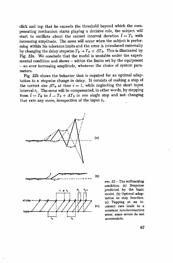
click and tap that he exceeds the threshold beyond which the com-pensating mechanism starts playing a decisive role, the subject willstart to oscillate about the correct interval duration î = TO withincreasing amplitude. The same will occur when the subject is perfor-ming within his tolerance limits and the error is introduced externallyby changing the delay stepwise T0 -»• T0.+ AT0. This is illustrated byFig. 22a. We conclude that the model is unstable under the experi-mental condition and shows - within the limits set by the equipment- an ever increasing amplitude, whatever the choice of system para-meters.

Fig. 22b shows the behavior that is required for an optimal adap-tation to a stepwise change in delay. It consists of making a step ofthe correct size AT0 at time i = \, while neglecting the short inputinterval h. The error will be compensated, in other words, by steppingfrom I = TO to I = TO + AT0 in one single step and not changingthat rate any more, irrespective of the input t\.

(a)

(b)

clicks

FIG. 22 - The selftrackingcondition, (a) Responsepredicted by the basicmodel, (b) Optimal adap-tation to step function.(c) Tapping at an in-correct rate leads to aconstant synchronizationerror, since errors do notaccumulate.

67

600

FIG. 23 - Responses to a stepwise change in delay (dashed curves) in selftrackingcondition. Time in msec.

This procedure may look simple, psychologically, for a trained sub-ject, but it is essentially incompatible with the model developed thusfar and requires a system which is psychologically not realistic. For,if the subject followed the optimal strategy shown in Fig. 22b, wewould have: $} = {0, 1, 1, 1, . . .} as a response to {tt} = {1, 0, 1,1, . . .}, and by Eq. (4.4a) we find

H(z) =T(z)

(4.19)

By long division of H(z) we arrive at {hi} = {1, 1, 0, — 1, — 1, 0, 1,1, . . .} which means that a single disturbance would bring the systeminto a state of sustained oscillation, a not very likely event to happenin a human subject.

68

1200

FIG. 23 (continued)

Comparison of the open loop function Eq. (4.15) with that derivedfrom Eq. (4.19),

G(z) =(*-!)«

(4.20)

shows that the two can never be equated whatever the choice of a andß. The following experiment was carried out to see how subjects copewith this incompatibility. If they adhere strictly to performance inaccordance with the model, their response will 'explode', i.e. theoscillations in interval length will go out of bounds.

Design

Three experienced subjects from the regular pool of subjects, B, vdVand M, and an additional much less trained subject, W, produced10 positive and 10 negative steps in response to a delayed feedback of

69

their own output intervals. The delay TO (= has) was either 600 or1200 msec while the stepwise increment was 32% in both conditions.The instants at which a step up or down occurred were determinedby the experimenter and were quasi-random.

Results and Discussion

In Fig. 23 the average response functions $} of each of the foursubjects are presented for — 2 ^ » ̂ 12. In the diagrams the largest,median and smallest standard deviations are drawn, which show howconsistent subjects - at least trained subjects - are in their quitepeculiar behavior.

It will come as no surprise that the subjects are able to adapt toa change in delay much better than is predicted by the model. Yet,the results show clearly that it is not an easy task. The size of over-shoots is much larger than in previous experiments and they extendover more intervals. The damping of the oscillations in the averageresponses of Fig. 23 is in fact even flattering since in separate trialssubjects generally did not reach a stable state at all (Fig. 24). Someof the apparent damping in the average response is due to sudden180° phase shifts in the oscillation (see Fig. 24), and some seems to bedue to the fact that subjects, every now and then, hit the right intervallength and then proceed to tap correctly.

2000r trial 8 triano

/\/V V\

1000

FIG. 24 - Persistence of oscillations in selftracking experiment, after stepwisechange in delay (dashed curve). Time in msec. (Subject B; 1200 msec).

Not in all responses do we find sustained oscillations. The adaptationis sometimes very gradual (Fig. 23; B600). This gives us a hint as towhat strategy is helping subjects to cope with their synchronizationdifficulties. This strategy is only applicable in the selftracking con-dition, since in previous experiments it would have lead to an everincreasing phase error. In the present situation namely, synchroni-

70

zation errors do not add and subjects are apparently able to use thisproperty of the experimental arrangement to reduce their synchroni-zation error gradually instead of trying to compensate for it as quicklyas possible. In some cases we observe a combination of protractedoscillation and 'creeping' compensation (Fig. 23; B1200, W1200). Anobservable consequence of the experimental situation is also that arest-state may be reached which differs from the actual delay interval :if the phase error is within the tolerance limits set by the subject, nofurther action will be taken to make the error smaller, since the timedifference between click and tap will not grow with each subsequentinterval (M600, vdV600). (Thus, this experiment provides a techniqueto study systematic errors in key tapping behavior.)

We conclude that a considerable revision of the model would berequired if it were to deal with the experimental situation in an appro-priate way. Obviously however, subjects also experience considerabledifficulties when they try to obey the instruction to maintain thesynchronization relation (Fig. 24), and this may indicate that theydo not easily abandon the habitual pattern of synchronizationperformance that is described by the model. How difficult the situationis, can also be inferred from the results of subject W, whose averageresponse is drowned in its huge variance.

Tapping appears to be a real skill, even if at first sight it does notseem worthy of that name.

7.2. Random modulation of the input sequence - Experiment 6

A different limitation of the timing system can be studied when it issubjected to a random gaussian input sequence, which in f act makes anypredictive action invalid and consequently the use of the dynamicproperties of the timing system superfluous. We may hardly expectthat human subjects under such circumstances will adhere to a uselessstrategy, and we are interested to see whether they will alter theirerror-minimizing strategy; and if they do, whether all adopt the samecourse of action. There is a number of feasible alternatives, which havebeen observed under comparable circumstances in other aspects ofbehavior. Subjects may, first of all, start reacting instead of synchro-nizing with the input clicks. This will result in an average delay whichis small - approximately 150 msec - with respect to the intervals underconcern (^ 500 msec). This strategy ensures a minimization of thevariation in the errors. Secondly subjects may start tapping at a

71

constant rate, with a correct or incorrect average, i.e. extracting theaverage of the input or not paying any attention to thé input sequenceat all. Thirdly subjects may try to copy the statistical properties ofthe input without trying to follow the exact time course of the input,a phenomenon which is well known to occur in guessing (e.g. Garner1962, p. 220L). There is in the fourth place the possibility thatsubjects do not try to compensate any error, but just 'copy' the lastinput interval ^_i, i.e. they still use their memory for the most recentinput interval, but give up the error compensating part of theirbehavior. And finally they may stubbornly adhere to performance inaccordance with the model and content themselves with very largediscrepancies between clicks and taps.

It is simple to distinguish between these alternatives. The crosscor-relation function C(k) between input and output and the variance ofthe output sequence contain all the necessary information. C(k) isequivalent to the autocorrelation function R(k) (Eq. (3.3)) except thatit compares two distinct series of data for lag k ^ 0, instead of oneseries shifted along itself.

Reacting will give a high C(0) since the average interval betweena click and the reaction to it will be much smaller than one interval.The expected variance a2 will be that of the input sequence, (cr2

t),plus the noise (a2j\r) contributed by the subject while producingintervals, plus the variance of the reaction time distribution (crB

2T).

The constant rate strategy will have virtually zero crosscorrelationwith the input and only a^ as variance; in fact it is identical tothe continuation condition of Exp. 1. The 'statistical copy' will show

TABLE 4 - Predicted crosscorrelation coefficients and variance of responsefunction $} for various response strategies, if the input sequence has a standardnormal distribution.

Strategies

Reacting

Constant Rate

Statistical Copy

Reproduction of tf-i

Basic Model

Predicted Values

C(0)

high +

0

0

0

0

C(l)

0

0

0

high +

high +

C(2)

0 a]

0

0

0

high —

°î

! + °L + °Za*

9 1 _ 2

Ü ~r~ Ot N

°î + a»3fff

72

no correlation with the input either, but will copy the input variance,added to a#. Reproduction of t^\ will show a very high crosscor-relation for lag k = 1, and have a variance equal to azt + GZN-The model-strategy finally, has a high correlation with t^.\, and ahigh negative correlation with tt-z since ^ ~ 2^_] —tf -% (Eq. (4.6)).It can be shown that in this case a*, = 3o .̂ These points have beensummarized in Table 4.

The following experiment was carried out to see which - if any - ofthese strategies is actually adopted by the subjects, when confrontedwith a random input sequence.

Design

Three subjects, M, N and vdV, of the regular pool and two naivesubjects L and Bo, took part in the experiment. Each produced aseries of 200 intervals in response to a random sequence of intervals

TABLE 5 - Crosscorrelation coefficients and standard deviations of response torandom normal input sequences.

Subject

M

N

vdV

L

Bo

t

60012002400

60012002400

60012002400

60012002400

60012002400

C(0)

.092

.041

.192

.015

.086

.079

—.017—.013.020

.248

.094

.032

.192

.100

.075

C(l)

.382

.849

.692

.844

.540

.672

.903

.935

.870

.456

.278

.247

.066

.724—.039

C(2)

.374

.036

.116

.242

.088

.052

.056—.145—.010

.021

.137

.140

.088

.047—.072

*l

91.7168.5286.5

53.7131.8301.1

73.9186.8300.2

86.7231.5459.9

111.1167.0265.4

C(k) for p = 0.01 : ± 0.181 (n = 200)

73

at each of three values of tav (600, 1200 and 2400 msec). A %2 - testfor normality gave tf = 10.91, for 10 df (0.50 < p < 0.75), and therange of the autocorrelation function R (k) of the sequence, variedbetween 0.120 and — 0.130 for O ̂ k ^ 15, which is nowhere signifi-cantly different from zero (but see note 2 on p. 34). The distribution ofthe input sequence was truncated at tav ± Q.2ßtav, i.e. at tav ± 2ff(.The actual standard deviations (st) of the input sequences were 58.6,117.2 and 234.4 for tav = 600, 1200 and 2400 msec respectively.

Results and discussion

The relevant data, the crosscorrelation functions C (k) for k — O, l, 2and the actual standard deviations s,, were calculated for each of thethree series of each subject and have been collected in Table 5.

The only tapping strategy which can account for the results, atleast those of the trained subjects, is the 'reproduction of t^\' : C(l) ishigh and positive, C (2) is virtually equal to zero except in one casewhere it is positive. The basic model in fact predicted C(0) = — 0.13,C(l) = 0.93 and C(2) = — 0.67 on the basis of the input sequencepresented.

The variance of the response sequence is assumed to be a compositeof the variance of the input plus the noise of the 'time sense' itself. Thetwo may be treated as additive since both are based on (quasi-) nor-mally distributed events. The input sequence was constructed thatway and in Chapter III the internal noise component was shown to beapproximately normally distributed. Hence we can make an estimateof s*if, which should be proportional to fi, since sy oc ôî oc î™. Thisestimate is of necessity very rough since the data are quite variable.We have therefore averaged over subjects M, N and vdV. The naivesubjects were left out of consideration: their performance clearlyfollows a different pattern, possibly affected by a learning effect.

TABLE 6 - Observed and predicted values of öl, in msec, under the hypotheses

'av

60012002400

si (observed)

73.1162.4296.1

ai (predicted)

65138325

ai (pred. Weber)

74148296

74

It turns out, that the additive relation szi =szt + s2jv does not

give a particularly good fit, when the 1.5-power relation is applied,not even when we assume on the basis of the results displayed in Figs7 and 8, that there is some negative correlation between li and li-\.Instead, if it is assumed that a normal Weber relation holds, a muchbetter fit is obtained, as can be seen by comparing the two relevantcolumns of Table 6.

We can offer no reasonable explanation for this evident deviationfrom the quite firmly established relation ôî oc î™.

With respect to our main objective, we conclude that the way inwhich subjects try to synchronize with a randomly modulated seriesturns out to be a fairly faithful following of the input, with a lag ofone interval. The naive subjects seem to have followed a much morerandom 'strategy', which was also confirmed by the calculation of theautocorrelation functions of the response sequences: no systematicsequential dependency was found in any of the series of data: R (k)unsystematically varied between + 0.200 and — 0.221 for O ̂ k ^ 15.

75

CHAPTER V - QUANTIZATION IN TAPPING

1. I N T R O D U C T I O N

In this chapter we shall deal in some detail with two points whichwere raised earlier and which might be interpreted as evidence forthe quantal structure of psychological time. The type of experimentsreported in this study is not suited to provide direct evidence for theexistence of a basic unit of time; this seems to be at least one pointwhere "the psychologist should yield his seat to the neurophysiologist"(Ehrlich 1958). We are interested in the phenomenon in view of ouraim of providing a descriptive framework of timing behavior, whichought to include any quantization of the output, whatever its source.

A quantized signal is characterized by the property that it mayassume only a finite number of values. Changes from one level toanother occur stepwise and abruptly. By quantization of time inter-vals we usually mean that intervals can be described as integralmultiples of some basic interval T, which is mostly said to lie in therange between 50 and 200 msec, (Stroud 1955) although shorter 'timequanta' have been reported (see for instance Latour 1961, 1966). Theevidence for the quantal structure of time has become quite weightyover the past 15 years (see Hirsh and Sherrick (1961) ; Lansing (1957) ;Latour (1966); Lichtenstein (1962); Mundy-Castle and Sugarman(1960) ; Stroud (1950, 1955) ; Venables (1960) ; White (1963) ; Whitrow(1960) and numerous other authors). Thé problem is clearly waitingfor a thorough, critical evaluation.

In our opinion this wealth of evidence has reduced rather thanenhanced the likelihood of finding a unit of psychological time.Instead it has become increasingly clear that perceptual and motorbehavior are necessarily quantal in character in order to make their'cortical control' possible. The analogy with the 'cycle time' of a digitalcomputer readily suggests itself (Latour 1966). In this setting any timeunit which is functionally appropriate will, under certain conditions,take the role of a 'time quantum' whether it be 20 or 120 msec long.The complexities with respect to the fundamental constituent periodici-ties appear at present to lie beyond our comprehension (Latour 1966).

76

We have found two manifestations of quantization in time intervalsproduced by key tapping: distributions of intervals produced bysynchronization or continuation show multimodalities which at firstsight seem to be periodic (Exp. 1 ; Fig. 10) ; and the adaptation tosmall average rates of change in sinusoidal input sequences showsindications of stepwise compensation of synchronization errors (Exps2 and 3). These two effects will be dealt with in the two sections tofollow.

2. THE M U L T I M O D A L I T Y OF TAPPING I N T E R V A L

D I S T R I B U T I O N S

Periodicities in the distributions of interval estimates have not beenreported in the literature. Multimodality has been found however inthe distribution of reaction times (Lansing 1957; Mundy-Castle andSugarman 1960; Venables 1960; Woodworth 1938). Distributions ofsearch times in detection tasks were also found to be periodic (Augen-stine 1955). Generally the periods reported are of the order of 100msec or bear a simple relation to that duration, which might be relatedto the alpha-rhythm of the brain. Most authors have been hesitantto formulate such a connection in terms of cause and effect. So muchseems clear however, that the observed multimodality is not a simpleartefact caused by the tremors of the extremity with which thereactions are executed : the frequency band of the latter is much widerthan was reported, for instance, for decision times by Augenstine(1955).

The reasons why no periodicities in the distributions of time inter-vals have been reported before seem to be simple : apparently nobodylooked for them and hardly any author has collected enough data toenable him to undertake a periodicity analysis of some kind.

The following analysis of the distributions of Exp. 1 was carried outto verify whether the observed fluctuations are periodic, and if theyare, to see to what extent they are stable over trials and conditions.

Method

The technique of autocovariance spectral analysis on discrete datawas used, as described by Blackman and Tukey (1959). This techniqueconsists essentially of two steps. First the autocorrelation functionR(k) of the time series to be studied is determined (Eq. 3.3). Thenext step is to fit cosine functions of increasing frequency v, to R (k). If

77

AT is the class- or sampling interval of the time series, then O ̂ v ^1/2 AT. The index of the fit of a particular cosine function is the sum of

the cross products of R(k) and the function^ = cos (— k AT) in which

p/2mAT is the frequency (O ^ p g m, and m ^ k). The expression

m-l _£V(p) = (R(0) + 2 £ R(k) cos^-k + R(m) cos np} AT (5.1)

for 0 ^ p ^ m, is called the raw spectral density at frequency v =pj2mAT. For example, the autocovariance spectrum will be flat -within certain statistical limits - if the original time series originatesfrom a random gaussian noise, the 'density' being a function of thevariance (bandwith) of the data. If on the other hand, the time seriesis a pure simple sinewave, R(k) will be a pure cosine function, andconsequently V(p) will consist of a single peak at a particular fre-quency.

Usually the spectrum is smoothed, using a relation like

U(p) = 0.54V(p) + 0.23 {V(p + 1) + V(p - 1)}, (0 < p < m). (5.2)

There are no completely satisfactory tests to determine whether aparticularly high peak in U(p) indicates a significant periodic trendin the data. Blackman and Tukey (1959) proposed a #2-test which isbased on the probability that a peak value in the spectrum is due tochance variations, given the overall variability of the spectrum. Thistest provides at least a reasonable indication of the importance of thepeaks in a spectrum.

Data

U(p) was calculated for all 32 series with interval length îav = 1667and 3333 msec of Exp. 1. Series with smaller values of îav could notbe used since the total range of their distributions was much less thanthe required value of approximately 10 times the expected largestperiod in the data. Even some of the 1667 msec series did not meetthis requirement, but in no case was a sample less than 800 msec wide.The intrinsic difficulty is that collecting more data will not appreciablyincrease the range of their distribution. We are helped however byhaving an estimate of U(p) from two independent samples on eachcondition. It should.be realized though that we are stretching the

78

requirements of the method to some extent, and that the results ofthe analysis are suggesting rather than establishing facts.

The sampling interval AT was set at 25 msec. Preliminary checksmade it clear that little information could be gained by taking ashorter, 10 msec, sampling unit (which in addition increased computingtime roughly by a factor of 10). Since spectral analysis requiresstationarity of the data, the distributions were modified in advanceby subtracting the expected frequency derived from Eq. (3.8) from theobserved frequency in each sampling interval.

o —

oo 400 200

FIG. 25 - Autocovariance spectra of the multimodal interval distributions ofExp. 1 (3333 msec synchronization sequences).

Results and discussion

The smoothed spectra U(p) and the significant peaks in U(p) weredetermined for each of the 32 series. The %2-tests were based on 4degrees of freedom.1 The results have been summarized in Figs 25and 26. Fig. 25 provides examples of the smoothed autocovariancespectra. It incorporates U(p) for all synchronization sequences ofti = 3333 msec for all four subjects. It is clear that there are peaksin the spectra which are significant. Accordingly there are periodic

1 The number of degrees of freedom, df, has been estimated from df =2 (Dn — Dm)/3Dm, in which D„ is the number of data points, and Dm is themaximum lag. In our case this amounts to 3 df, to which 1 df has been addedas a (conservative) estimate of additional degrees of freedom due to peaks in thespectrum (Blackman and Tukey 1959).

79

- n = 15

in ro CM CM

q qö ^o o>

81.4

85.5

78.2

6

4

2

0

12

10

8

6

4

2 -

M

n = 1179.4

JU!

n = 47

Md =81.0

Q, =93.0

l . l '_:

10 14 16 18 20

FIG. 26 - Distributions of significant peaks in the autocovariance spectra of theinterval distributions of Exp. 1.

fluctuations in the distributions of the longer intervals of Exp. 1.However, there are frequently peaks at more than one point and insome cases there is a fairly high spectral density over a quite broadpart of the frequency range. In the third place it looks as if in somecases the spectrum of the second series is shifted slightly with respectto the first (Fig. 25).

Since the spectral densities were estimated from very short samples

80

we can base no firm conclusions on these observations. It is clearhowever that he who wants to find a singular unit of psychologicaltime will look in vain. Depending on the momentary situationdifferent period lengths may be observed, suggesting that the timequantum is a functional rather than a deterministic entity.

Notwithstanding the variation in the values of the 'time quantum',we can see in Fig. 26 that there is a quite marked central tendency forthe significant peaks (5% level or better). They cluster around amedian value of 81 msec, with an inter-quartile range of 20 msec.Fig. 26 shows the distribution of these peaks for each subject and forall subjects together. Of the 47 significant peaks 27 fall within ± 10msec from the median. Furthermore subject S showed consistently asecond peak at approximately 105 msec, thus contributing most to thepeak at that value in the combined graph. Neither in this, nor in anyother case, was there any indication that the peaks in one and thesame spectrum bear a simple relation to one another: peaks do notshow at integral multiples of a particular frequency. We did notfind, finally, any significant differences in the distribution of thepeaks between the continuation and synchronization series (medians82.5 and 78.3 msec respectively), or between the 1667 and 3333 msecinterval lengths (medians 78.0 and 81.7 msec respectively).

It was suggested earlier that the size of the time quantum depends onthe prevailing circumstances. If this is so, neither the length of theinput intervals, nor the input mode, seem to be determining factors.The following section will give some indications as to what kind offactors is important.

3, STEPWISE ADAPTATION TO A M O D U L A T E D INPUT -

E X P E R I M E N T 7

Quantization of time intervals should be observable in the responsesto modulated input sequences. To the extent that adaptations to aconstant rate seem to be carried out stepwise, we may expect thatsuch steps can also be observed if the length of the input intervals va-ries slowly enough. Sinusoidal modulation provides low rates of changebut tends to have any quantization effect wiped out, since the stepswill become desynchronized in absence of clearly marked anchorpoints in the input sequence. Experiment 7 was designed to providesuch anchor points and to enhance quantization effects if present at all.

81

Design

Two subjects, M and vdV produced two series of 10 accelerated and10 decelerated sequences of the 'ramp functions',

t

*

and

, [I

i < 0+ kAt, »^ 0

+ 200, » < 0+ 200 - kat, 0

(5.3)

(5.3a)

in which has = 600 or 1200 msec, At = 10 or 20 msec and A = 20 or 10respectively (kAt being maximally 200 msec.). The results of eachseries of 10 trials were averaged, whence two average responses oneach of the 8 conditions were obtained. Steps in the adaptation to thechanging rate were determined graphically, a step being identified bytwo conditions of the first differences between any two successiveintervals: | Att \ > \ A^i \ n | Aît+i \, and Al^-\ ~ Ali+i ~ 0. At veryfew points did this decision criterion fail, although some arbitrarinesscould not always be avoided (see Fig. 27).

800

700

600

eoo

700

600

•30—1-20 H

v. d. V. ; 10 msec, steps

I 80 1—60—1

M.; 20 msec steps

FIG. 27 - Examples of responses to ramp function input with low rates of change.Time in msec. The dashed line represents the input function.

82

Results and discussion

Quantization or stepwise adaptation was very prominent in virtuallyall of the records. There were one or two exceptions in the 600 mseccondition only. The steps can be characterized by two measures,their heights and widths, which need not be completely reciprocal,though they are closely related. Height and width of each step in therecords were estimated and are represented in summary in Table 7.Since there were no significant differences in performance betweenthe two subjects, their results have been combined.

TABLE 7 - Average height (msec) and width (number of intervals) of steps instepwise adaptation to ramp function input with small At. (Means and standarderrors).

At(msec)

1020

Width

3.733.18

±±

0.150.24

600

t d as (msec

Height

36.766.9

±1.53±4.75

4.3.

)

Width

03 ±19 ±

0.380.22

1200

Height

46.367.0

±±

2.354.72

The outcome is consistent with the findings reported earlier, in oneimportant respect : the step height is approximately the same for thetwo values of ^ag. This indicates that the adaptation is essentially-carried out on the basis of the prevailing error rather than on theaverage length of the intervals. The difference of a factor of two instep height - and accordingly the identical width of the steps - in the10 and 20 msec conditions is less obviously related to our earlierfindings. The only explanation which is consistent with the obser-vations, is that subjects maintain approximately a constant rate oftapping, and update their response after a more or less fixed numberof intervals, irrespective of the actual synchronization error e, as longas that error is not large in comparison with the fluctuations (ôî) inthe estimates of t. This kind of behavior is not unusual in psycho-physics. Subjects seem to postpone a decision as to what action theywill take, until they have accumulated sufficient evidence about thenature of a stimulus - in our case the synchronization error.

If on the other hand the difference between click and tap is farabove threshold, the uncertainty of the subject will be reduced instan-

83

taneously, and a much more continuous adaptation to the inputsequence will result, as we saw in most of the preceding experiments.Further experiments may reveal in greater detail the properties of thedecision process which underlies the 'intermittent adaptation' toslowly changing input rates.

4. C O N C L U S I O N S

The question if there is a universal time quantum of virtually fixedsize r, does not appear to be any closer to an affirmative answer thanit was before. We have found step effects in a range between 25 and125 msec, with only one characteristic in common : the step size remain-ed fairly constant within an experimental condition. This supportsthe view, expressed earlier, that each specific situation may have itsown functional 'processing time unit' which may vary widely fromsituation to situation. Yet, we predict that steps much smaller than25 msec are unlikely to occur in the type of behavior under investi-gation, even if the motor system is able to produce finer adaptations.Below 25 msec we are in the range of durations where the order oftwo successive events cannot be determined any more (Hirsh andSherrick 1961). Even if the size of the error could be estimated reliably,the subject would not be certain as to whether he should increase ordecrease his rate of tapping. Consequently he would wait for ad-ditional information during later intervals, before correcting his rate.

Finally, it seems that most of the quantization phenomena in ourexperiments are a result of the effect of a threshold mechanism ofsome sort (perceptual or cognitive) on the dynamic 'time sense'. Atthe same time, it is not entirely clear how the periodicities found in theinterval distributions of Exp. 1 tie in with the concept of such a thresh-old. Whether these periodicities and the 'intermittent correction'derive from the same process remains open for further investigation.

84

CHAPTER VITHE INFLUENCE OF NON-TEMPORAL INFORMATION ON TIMING

1. I N T R O D U C T I O N

In Chapter I some of the work pertinent to the effects of non-temporalfactors on time perception and timing was reviewed. We will concludethe experimental part of this study with three exploratory experi-ments, dealing with the influence of what we named 'informationprocessing load' on the timing system. This problem is not onlytheoretically of interest but has considerable practical importanceas well. Since transmission of information is gradually replacingtransmission of energy in human jobs, there has been a growing con-cern for the extent to which the information transmitting channelsof industrial and military personnel are occupied by the requirementsof such tasks as, for example, process controling in an automaticfactory.

It is possible to measure how far the processing channel is occupiedby a particular task, by means of an extra task which has to be per-formed concurrently with the main task. Some index of deteriorationof performance on the secondary task is then used to classify tasks inorder of the load they impose on the worker (see e.g. Bartenwerfer,Kotter and Sickel (1962); Bertelson et al. (1966); Knowles (1963);Koster and Taverne (1966); Schouten, Kalsbeek and Leopold (1962).)The present author demonstrated elsewhere (Michon 1964a, 1966a, b)the usefulness of an index of irregularity of tapping at the 'personalrate' as a measure of information processing load.

In the literature we find some disagreement as to whether theperformance decrement of the secondary - and frequently the main -task is due to interference between parts of the simultaneously pre-sented information or to intermittent processing of information fromthe two tasks. Of the two possibilities the latter seems to be the mostattractive alternative. Much evidence has been accumulated in supportof the 'one channel hypothesis' of human information transmission onwhich it is based. According to this view - put forward by Hick (1948),Broadbent (1958) and other British psychologists (Davis 1957; Wei-ford 1959, 1960; see also Sanders 1963, 1967a, b), - human oper-

85

ators can extract information from only one source at a time. Multiplesources have to be dealt with by 'switching' more or less frequentlyfrom one source to another, i.e. by intermittent processing. Theprocess of switching (see Egeth 1967; Sanders 1963, p. 261; 1967b)was originally thought of as peripheral or 'sensory 'switching, but seemsgradually being replaced by a more 'functional' switching concept, inwhich the nature of the information source is entirely determined bythe characteristics of the task. We might have, for instance, switchingbetween a meaning-source and a spatial location source. The mostup to date review of the various problems of the one channel hypoth-esis can be found in Welford (1967) and other papers in Sanders

The use of key tapping as a secondary task is based on the assump-tion that temporal information has to be processed like any other kindof information : the duration of intervals has to be stored, retained andretrieved, and it has to be compared with other stored intervals orwith running clock time. By stressing the timing aspects of work, theuse of tapping as a measure of information processing load brings usclose to the research in which response latencies and decision times aredescribed in terms of queuing models (Kaufmann 1963 ; McGill 1963 ;McGill and Gibbon 1965; Restle 1961; Restle and Davis 1962). Thepsychological applications of queuing theory do, however, not includemultiple source models thus far.

The aim of the following three, minor, experiments is to gain somepreliminary insight into the effect of non-temporal information on thetiming system. One point is of particular interest in this context.As we said before, the regularity of timing performance is affectedmarkedly when it is measured under the 'double task' condition, i.e.when key tapping is given as a secondary task. In that case the twotasks are presumably functionally independent, and carried out alter-nately. In most practical circumstances however, the timing aspectsof a task will be integrated with its non-temporal aspects. In musicalperformance, for example, timing or rhythmical information is coded

1 It should be stressed incidentally that in the work on human informationprocessing which makes use of computer simulation, the one-channel hypothesisis an implicit postulate. The design of present day computers embodies only one'accumulator' through which all information is manipulated. The accumulatoris unable of "doing two things at once". In this kind of research little explicitattention has been paid thus far to the properties of the human 'accumulator'processes, like attention and short term memory.

86

together with information about melody, accentuation and intensity.Although it is likely that the latter will exert appreciable influences onthe former categories, the major switching problem, which would ariseif we tried to play the piano and to recite an entirely disconnected pieceof prose simultaneously (Pauli 1937), is absent under the 'integratedtask' condition.

2. SEPARATE VS. I N T E G R A T E D PROCESSING OF TEMPORAL AND

N O N - T E M P O R A L I N F O R M A T I O N - E X P E R I M E N T 8.

The following experiment was carried out to see if the synchronizationresponse is affected differently when extra information is processedunder double task conditions than it is under integrated task conditions.

In this experiment - and also in the following two - the temporalstimuli, sequences of auditory clicks at 45 db above threshold, werepresented as before. In addition visual stimuli were presented whichwere selected randomly from sets of up to eight alternatives. Thestimulus arrangement consisted of a horizontal row of eight greensignal lights which lit up, one at a time, in a random sequence whichhad been prepared on punched tape. The punched tape reader was inturn activated by a signal from any one key of the set of responsekeys in front of the subject. The schematic diagram of the arrange-ment is shown in Fig. 5 (see p. 25). Upon pressing any of the keys ofthe set, a new stimulus was presented without delay. Subjects wereinstructed to watch the stimulus, select the appropriate response key- always with full left to right compatibility - and to press the selectedkey in synchrony with the clicks presented through the headphone, inone condition (integrated task). In the second condition they did notsynchronize by means of the set of response keys, but tapped a Morsekey, as in the earlier experiments and responded to the visual stimulibetween successive taps. The tapping was performed with the righthand, the reaction keys were pressed with the left hand.

Design

Three of the regular subjects (vD, B and M) took part in this experi-ment. One, vD, may be considered a very consistent performer, while.B did show the largest variances throughout the experiments. M tookan intermediate position in most experiments.

Each subject was presented with two series of 10 positive steps with

87

tbas = 1200 msec and stepwidth At = 192 msec (16%). Non-temporalinformation consisted of randomly selected lights from a set of four(the central four of the row of eight), which is equivalent to an eventuncertainty of 2 bits.

Results and discussion

The average responses were determined for each series of 10 steps.The results are shown in Fig. 28, separately for all three subjects.

ior B

5-

0 2 4 6

FIG. 28 - Average response to positive step function input under influence ofnon-temporal information in the double task condition (b), and integratedtask condition (d). (a) represents distribution of the instants at which responsesteps are initiated with respect to the input step, (c) shows the result of rear-ranging the response trials on the basis of (a).

Three conclusions may be drawn from the results. Although, in thefirst place, there is a considerable difference between the averageresponses in the two conditions (Fig. 28 b and d respectively), much ofthe difference can be explained from the variable delay in onset of

88

the compensatory action. In the double task condition our subjectsdid not necessarily compensate for the change in rate at instant i = 1,(the step being presented at i = 0) but the adaptation could occur atany instant i = 1, . . . , 5, as is shown in Fig. 28 a. If we rearrange theseparate trials is such a way that the points at which the actual tran-sition in the response is made coincide, we obtain the average responsecurves shown in Fig. 28 c. The latter curves come much closer to thosedepicted in Fig. 28 d, which suggests that the system response in itselfis not too different under the two experimental conditions but thatin the double task condition subjects have to surmount a higherthreshold or level of uncertainty before they decide to adapt to a newrate, (see Sec. V. 4).

A second conclusion to be drawn from the results is that in theintegrated task condition the responses of the three subjects comparevery well with the responses produced in absence of non-temporalinformation (see Fig. 19). Hence we can conclude that the effect ofthe non-temporal information is on the variability of the results,rather than the average response; in fact we may attribute the shiftin the point of transition to increased variability as well. The varia-tions in the average response were found to be of the order of ôî ~ 0.090for iav = 1200 and ôî ~ 0.120 for lav = 1400, averaged over the threesubjects. Comparable results for performance in a comparable situa-tion without non-temporal information can be derived from Fig. 20,where we find ôî ~ 0.060 and ÔÎ ~ 0.075 for l„ = 1200 and 1400respectively.

Thirdly, we find that subjects differ considerably from one anotheras to the extent to which they are affected by extra information (Fig.28a, for instance, shows this), which is a common finding in studiesabout 'information processing capacity'.

3. I N V A R I A N C E OF THE A V E R A G E RESPONSE - E X P E R I M E N T 9

This experiment is intended as a further check on the response invari-ance of synchronous tapping in the integrated task condition. If suchresponse invariance exists, irrespective of variations in the amountof non-temporal information, we may assume that the timing systemis not directly affected by extra information - in the sense that thesystem parameters change - but that momentary fluctuations, mainlythose which may affect the memory for intervals or the appreciationof synchronization errors, are increased. In other words : if the average

89

response is invariant, the non-temporal information affects thosecomponents which manifest themselves as (quasi-)noise.

Design

Each of four subjects, vD, B, M and vdV contributed two series of10 steps up and down at tbas = 1200 msec and At = 192 msec (16%),with 2, 4 and 8 alternative choices (see Exp. 8) as extra information,under the integrated task arrangement. As before, the occurrence ofthe steps was randomized to preclude anticipation by the subject.

1200 B + 1200

a= 0.80ß = 0.88

1200

l/ <x = 0.88y ß = LOOFIG. 29 - Average responses to a step function input under influence of non-temporal information in the integrated task condition. (2 ( x ), 4 (•) and 8 (+)alternative choice task).

Results and discussion

The response functions are shown in Fig. 29, which makes it evidentthat there is no effect whatsoever of the amount of extra informationon the average response, and consequently on the system parameters.The only exception seems to be subject B, who displays a decrementin overshoot with increasing extra information, and a correspondingincrement of the overshoot at a later instant (i = 2). Unlike the effectobserved in the previous experiment (Fig. 28 a), this shift in response

90

is not due to variations in the instant at which the change in tappingrate is effectuated: in all trials except two, the step in the responseoccurred at instant i = 1.

TABLE 8 - Analysis of the fit of previously estimated parameter values (Exp. 4)to data of Exp. 9 (see Table 3).

Subject Parameters

vdVBvDM

a

0.920.800.880.76

ß

1.000.881.000.84

Var. Red. (ILP

Expli-cable

79.252.5

—54.061.9

Exp'nd

64.835.3

-41.349.5

= 100)

Exp'ndExp'ble

0.820.670.770.80

Sign, of Residual

F P (%)

6.32 <.0013.68 <.013.78 <.013.33 <.01

2633

The response curves (solid lines) which were drawn in Fig. 29 arethe same as the curves drawn in Fig. 19 for t^as = 1200 msec. Thisenhances, in a way, the response invariance: all curves give a quitegood fit for the data of the present experiment. The amounts ofvariance explained by the parameters estimated in the earlier ex-periment (Exp. 4) are given in Table 8, and compare excellently withthose of Table 3, at least for three of the four subjects. The perform-ance of vD was explained more adequately by chosing a = ß = 1,i.e. by the basic model. It seems likely that a substantial improvementof the fit might be achieved - like we suggested in the discussion ofExp. 4 - only by modifications in the model rather than by a betterestimate of the two parameters.

Further comparison of Figs. 19 and 29, and of Tables 3 and 8, showsthat the effect of the step width (Exp. 4) is more detrimental to theinyariance of the response function than is the amount of non-temporalinformation - at least within the modest range of the conditions studied.

4. THE EFFECT ON THE RESPONSE TO I S O C H R O N I C I N P U T

SEQUENCES - E X P E R I M E N T 10

In this experiment we have tried to determine what the effect is ofnon-temporal information on the noise components of the timingresponse. Thus, we return to the input conditions of Exp. 1 (Chapter

91

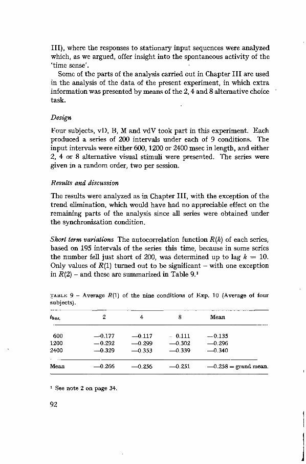
Ill), where the responses to stationary input sequences were analyzedwhich, as we argued, offer insight into the spontaneous activity of the'time sense'.

Some of the parts of the analysis carried out in Chapter III are usedin the analysis of the data of the present experiment, in which extrainformation was presented by means of the 2, 4 and 8 alternative choicetask.

Design

Four subjects, vD, B, M and vdV took part in this experiment. Eachproduced a series of 200 intervals under each of 9 conditions. Theinput intervals were either 600,1200 or 2400 msec in length, and either2, 4 or 8 alternative visual stimuli were presented. The series weregiven in a random order, two per session.

Results and discussion

The results were analyzed as in Chapter III, with the exception of thetrend elimination, which would have had no appreciable effect on theremaining parts of the analysis since all series were obtained underthe synchronization condition.

Short term variations The autocorrelation function R (k) of each series,based on 195 intervals of the series this time, because in some seriesthe number fell just short of 200, was determined up to lag k — 10.Only values of R(l) turned out to be significant - with one exceptionin R(2) - and these are summarized in Table 9.1

TABLE 9 - Average A(l) of the nine conditions of Exp. 10 (Average of foursubjects).

Mean

8 Mean

60012002400

—0.177—0.292—0.329

—0.117—0.299—0.353

—0.111—0.302—0.339

—0.135—0.296—0.340

—0.266 —0.256 —0.251 —0.258 = grand mean.

1 See note 2 on page 34.

92

An analysis of variance on the complete set of values R(l) confirmedthe conclusion to be drawn from Table 9 that no significant differencesbetween the 2, 4 and 8 alternative conditions exist. There are signifi-cant differences, however, between the various t^s, a tendency whichwas not obviously present in the data of Exp. 1, and which wasconsequently not explicitly analyzed in Chapter III.

The grand mean of the R(i) of all 36 series is Rav(l) = — 0.26, witha standard deviation of 0.131. This is not significantly different fromthe mean of the R(l) of the autocorrelation functions in Exp. 1 (Fig. 7)which was — 0.20 (with standard deviation 0.073). A Student t-testgave t = 1.80 for 23 degrees of freedom.

The conclusion from these results is that a produced interval isneither more, nor less, dependent on preceding intervals as a resultof extra information than we observed in Exp. 1. This may be takenas additional support for the conclusion drawn in the discussion ofExp. 9, that the system parameters are not affected by non-temporalinformation.

Extreme deviations. The analysis of extreme deviations, carried outon all 36 series, leads us to another piece of evidence for this contention.The results are summarized in Fig. 30, which is directly comparableto the contents of Fig. 8. The response curves for the local behavioraround deviations which exceed two standard deviations with respectto the local mean, are self-evident : again we do not find any significantdifference between the 2, 4 and 8 alternative conditions, a result alsoconfirmed by an analysis of variance.

3

21

o-1

-2

FIG. 30 - Compensation of extreme deviations under influence of 2, 4 and 8alternative choice task in the integrated task condition. (600 (o), 1200 (•) and2400 (+) msec intervals).

The distribution of response intervals under various information loads.Under this heading the remaining part of the analysis in analogy

93

with that of Exp. 1 will be subsumed. A summary of those resultswhich are of interest to the problem tackled in the present chapteris given in Fig. 31 and Table 10.

With respect to the shape of the distributions we find again thatthere is a reasonable closeness to normality. Although no completeset of #2-tests was carried out on all 36 series, it appears from the£2-estimates that were made, that about 30 distributions will notdeviate significantly from a normal distribution, when the numberof class intervals is approximately 20.

The interval distributions show a much less pronounced tendencyto periodicities superimposed on the main shape, and accordingly thespectra were much less peaked. Again, the amount of data on whichthe spectra were based was too small to give more than a roughimpression, but the result of the extra information seems to be twofold:the peaks are much broader and their maxima vary over a wider range(the interquartile range being of the order of 45 msec, as compared to20 msec for the results obtained in Sec. V.2.). We will not go into anydetail with respect to these data, but they are, to say the least, notin contradiction with our earlier supposition that much of the quanti-zation effects in timing may result from an interaction betweenthe intrinsic noise of the tapping response and the evidence a subjectneeds for a proper functioning of his compensating mechanisms.

The relation between the standard deviation and the average lengthof the response intervals is illustrated in Fig. 31, which shows that theeffect of non-temporal information on the variability of the results isquite noticeable, with two restrictions though. Only at 600 and 1200msec do we find an effect (this is not an artefact of the logarithmicgrid of Fig. 31).

Not all four subjects show an equally large effect. As we might ex-pect, subject B showed a considerable deterioration, whereas vD andespecially vdV generated a much smaller increase in their variability.This was confirmed by an analysis of variance on log-transformeddata, showing that the overall effect of the number of alternatives issignificant (F = 12.62, 2/12 df, p < 0.001) but also that the size of theeffect is significantly different for different subjects (F = 3.23, 6/12df.p <0.05).

In order to see if the general trend of decreasing (relative) effect ofextra information at longer intervals, on the variability can be explainedby assuming that the processing of temporal and non-temporal in-formation is serial, the variance of the response intervals was compared

94

100

50

20200 500 1000 2000 5000

FIG. 31 - Variability of the response to isochronic input sequences as a functionof the average output interval length, for different amounts of non-temporalinformation (2 ( x ), 4 (•) and 8 (+) choice task. If variances would be additive,the data points would lie on the curves 2, 4, and 8 respectively.

with that of the interval distributions produced without extra infor-mation and the variance of the reaction time distributions of the 2, 4,and 8 alternative choice task. The assumption - undoubtedly an over-simplification - was that the variance of the choice reaction times properand the variance of the response intervals proper, will simply add tothe variance of the integrated task results, if the processing of thetwo kinds of information is completely independent, i.e. serial. Apresupposition, in that case, is that much of the preparatory action tothe actual processing - i.e. the conduction to an from the central parts ofthe nervous system - occurs simultaneously. Otherwise it would beimpossible that the time to deal with both tasks is much less than thesum of the average response times for the separate tasks. In otherwords it is supposed that most of the variance is contributed by proc-esses which have very short average latencies but high variability.

A test of the extent to which the variances of the response intervalsand the reaction times of the choice tasks add has been summarizedin Fig. 31, which in part is based on the data presented in Table 10.Table 10 derives from the reaction times of the four subjects who tookpart in Exp. 10, in response to random sequences of stimuli. 50reactions were obtained in the 2, 4 and 8 alternative conditions, undereach of two instructions. Subjects produced these reactions in a selfpaced situation, either under the instruction of working as fast aspossible without making errors (Quality), or with an instruction towork as fast as possible, not paying attention to errors (Speed). The

95

TABLE 10 - Means and standard deviations of reaction times of 2, 4 and 8 choicereaction tasks. (Average of four subjects).

Altern.

2

4

8

Instruction

QualitySpeedQualitySpeedQualitySpeed

% Errors

3.517.51.0

18.02.0

18.5

Mean RT(msec)

463418582481702582

.„

323536454850

results of the four subjects were combined and are shown in Table 10,which reveals that the variance is not much affected by the two in-structions, whence they are combined in the following calculation.

The straight line with slope 1.5 shown in Fig. 31 represents theexpected relation between dl and îav in case there were no effect ofthe extra information. The curves identified by numerals 2, 4 and 8show the relation that would hold if the variance of the response inter-vals and the reaction times would be simply additive. The actualresults fall in between these two limits. A rough estimate of the corre-lation which is indicated by the data points in Fig. 31 was obtained fromthe relation for the sum of the variances of two normal stochasticvariables :

o't == <r* + <r* + 2r Oiat. (6.1).

We find that the correlation between the two variables is of the orderof r = ~ 0.25, which suggests that there is at least a moderate inter-action between the processing of temporal information and non-temporal information. The precise nature of this interaction remainsto be uncovered by further experiments.

5. C O N C L U S I O N S

This exploratory survey of the relation between non-temporal infor-mation and synchronization or timing has opened up many questionsabout the quantitative relations between temporal and non-temporalinformation, of which the previous sections offered only a provisionaloutline.

96

We found that timing performance is different when the relevantaspects of a task can be integrated with the processing of temporalinformation, than when that second task is executed as a secondarytask. In the former case the extra load is easily disruptive of the timingresponse, while in the latter case such an influence is virtually absent.With respect to the practical problem of measuring information proc-essing load this confirms that the use of extra load in the form of asecondary task is something fundamentally different from adding adimension within a task. The latter is in fact the approach of, amongothers, Conrad (1955) and Sanders (1963), as was pointed out by thepresent author (Michon 1966b).

Looking at the response to the isochronic input sequences, againlittle effect of non-temporal information was found on the dynamicaspects of the timing system. Those parts of the analysis which wereintended to bring to light any sequential or compensatory aspects ofthe response, as expressed in the systems parameters, were negative.The only effect of the extra information appears to be on the 'noise'generated by the subject. Incidentally it should be stressed that thisfinding does not necessarily allow extrapolation to very high levels ofextra load.

A simple essay to account for the effect of extra information on thevariability in the isochronic response intervals makes it likely thatthe temporal and non-temporal sources of information do interact tosome extent. A correlation, r ~ — 0.25, obtained from the data in-dicates that processing is in part serial, in part integrated.

97

CHAPTER VII - RECAPITULATION AND CONCLUSION

1. I N T R O D U C T I O N

In this final chapter we shall provide a summary of the various aspectsof the timing system as it emerged in the preceding pages, by stating itin the form of an information processing model. By doing so we reachback to the preliminaries of Chapter I, where we stressed the feasibilityof applying the information processing approach to the present problemarea. The basic, non-sequential, constituents of the 'time sense' wereput together in de diagrams of Figs. 1, 2 and 3, but we postponed theincorporation of a dynamic error compensating component in thesesimple diagrams for lack of relevant data. Building on the argumentsof Chapter I we will complete our model now.

In its final form it is put to a test by implementing it as a simpleprogram for a digital computer. Computer simulation has added apowerful new dimension to psychological methodology because itprovides a means of testing the logical consistency of a model ortheory and of checking if it functions in accordance with the intentionof the theorist (Feigenbaum and Feldman 1963 ; Newell and Simon 1963 ;Reitman 1965). We should consider the simulation of the 'time sense'solely as a formulation of the model in terms of a set of instructionsto the computer and not as an attempt to simulate the actual processesgoing on in the living organism. Writing a program only means:specifying our model in unambiguous terms, hence leaving open thepossibility of evolution out of its current state as well as the possibilityof falsification. The strength of computer simulated models is thatthey are particularly vulnerable with respect to the latter point.

2. FIVE FEATURES

This section is a summary of five main features of the experimentalresults.

(a) Memory for previous input intervals. It was found that subjectsact on the basis of knowledge about the sequence of input intervals.

98

This applies - mutatis mutandis - to external as well as internalstandards. In the latter case we may conceive of the standard as a'running average' of a small number of intervals previously producedby the subject, though it was not possible to determine just whatnumber.

(b) Memory for previous synchronization errors. Phenomenologicallythere is a second aspect involved in synchronization. Subjects activelymatch their taps with the clicks they hear and try to minimize thetime difference between click and tap - which, in fact, is exactly whatthey were instructed to do. The experimental results have added sub-stantial evidence for this compensatory aspect in timing behavior.

From the interaction between these two factors, essentially theretention of intervals and the concurrent retention' of synchronizationerrors, results the behavior which is described by the dynamic modeldeveloped in Chapter IV.

It is immaterial to the mathematical model how the contributionsof each of the two components of the 'time sense' are weighed in theequations which describe the behavior of the system. Expression Eq.(4.17) for instance gave the values of £< for any i ^ 0, as a function ofpreceding intervals, ^_i, t^z, • • • , ^-5, but 4 can equally well be ex-pressed in terms of a weighed error term, as in Eq. (7.1) :

{(1 — 2a) At t_i + (3a + 2b — 4«2 — 2ab)( — a — b + 8«2 + 9ab + 2b2) At^3 + (— 5az — 8ab —

(fla _|_ 2ab + &2) Aft.*}. (7.1)

Hence it seems to be a matter of some arbitrariness when we decide toattribute to the interval-memory sub (a), only the power to retain thelast input interval. This is consistent with some of the subjects'behavior however. In Exp. 6, and to some extent also in Exp. 5, wefound that the intervals produced by experienced subjects were afairly faithful copy of the immediately preceding input interval inthose circumstances where error compensation was not an appropriatestrategy anymore, to obtain a maximum of synchronization. More-over, when we deal with isochronic series of intervals there is no dis-tinction between keeping one interval in memory and retaining anynumber of input intervals, since all are identical. Finally, in thoseconditions where the 'ideal linear predictor' (Sec. IV.3) provides amore or less adequate description of behavior, it is only the last input

99

interval t^,\ and the last synchronization error e$_i which determinethe response of the system.

It should be stressed once more though, that finally the choice ofweights is a matter of psychological interpretation of a psychologicallyindifferent, formal model.

(c) Random fluctuations vs. average response. The first two features ofthe 'time sense' refer to the average response of a subject, based on anumber of independent trials with the same input function. Fluc-tuations in the response during a particular trial were neglected in thedynamic model and were not expressed in the model parameters. Wefound the short term fluctuations to be very nearly normally distrib-uted with a standard deviation which is proportional to the 1.5power of the average interval length îav. This relation can be inferredalso from a number of older studies (e.g. Stott 1933; Woodrow 1932;see also Michon 1964b, Fig. 1).

It was hypothesized - in a very preliminary way - in Sec. III.3 thatthis 'noise' may be due to a degradation of the 'internal representation'of an interval stored in memory. This memory decay would be pro-portional to the time elapsed since the moment of storage and byamounts reflecting a constant relative sensitivity (Weber's law).

In terms of information processing the random factor affecting thememory for temporal information represents a complex of factorsabout which we are ignorant. The results of Chapter VI suggest thatthe variability in synchronization may be caused by intermittentprocessing of temporal and non-temporal sources of information. Thismight also apply when no specified extra information is presented toa subject. We find that attention will wander during an experimentalsession, even with the most reliable of our subjects, and there is no apriori reason to make a distinction between externally and internallygenerated information with respect to intermittent processing.

Hierarchically the noise factor seems to be very much subordinateto the essential activity of the timing system. In particular, subjectswere frequently disturbed about their obvious inability to cope withthe quite considerable deviations they generated spontaneously whilethey were trying to track an isochronic input sequence.

(d) Thresholds and decision criteria. A fourth group of factors, foundactive in the timing behavior of our subjects, consists of two psycho-logically distinct but functionally equivalent types of entity.

100

There are lower limits on performance, usually set by the physio-logical limitations of the subject, and other limits whose transgressionmay drastically alter observable behavior but which are not thresholdsin the usual sense of the word. Frequently limits of the second kindwill even be quasi-cognitive. An example of the first category is thethreshold for perception of order, which plays a role in the stepwiseadaptation to very small changes in the rate of input (Exp. 7). Con-tinued error sampling in the case of small errors in synchronizationand the decision to abandon error compensation altogether when theinput modulation becomes essentially unpredictable, belong to thesecond category.

Such decision rules are crucial elements in information processingmodels; they determine the 'transfer of control' between parts of themodel on the basis of the results of operations carried out by thoseparts. Their number is in principle unlimited since they are establishedor at least influenced by all kinds of environmental, motivational andinstructional factors. Some will be inherent to the human organismand show up in some form in all subjects, others may be strictly perso-nal. Their number is ultimately restricted only by the level of analysisset by the investigator.

(e) The influence of non-temporal information. We have found supportfor our contention that the actual performance of the timing system(as determined by the basic properties of the model and the parametervalues) is not easily affected by non-temporal information. It seemsto be primarily the quality of the retention of intervals which is affected.

The precise relations between the - intermittent ? - processing oftemporal and other information remain to be established. Since wedid not arrive at quantitative formulations about these relationships,we will refrain from incorporating them in the present formulationof our model.

3. AN I N F O R M A T I O N PROCESSING MODEL OF THE 'TIME SENSE*

The final formulation of the model describing the timing behavior ofsubjects in a key tapping situation embodies the first four constituentfactors listed in the previous section. The present description adheresclosely to the simple processing models depicted in Figs 1, 2 and 3 ofChapter I, in addition to being a description of a computer program,written in the Digital Equipment Corporation version of FORTRAN n,

101

and run on a DEC PDP-7 computer with an 8000 word core memory.As before, it is possible to make a distinction between the functional

structure of the model and the actual flow of information between thecomponents.

3.1. The functional structure

The functional layout of the model is given in Fig. 32. The part at theright represents the 'time sense' of the subject, the part at left standsfor the essential elements of the experimental situation, the stimuluspresentation and recording equipment, and a 'physical clock'. Thesubject monitors the clicks presented to him and the taps which hegenerates himself on the basis of his 'internal representation' of theinterval to be produced (his prediction). This internal representation ismore complex than the interval memory of Figs 1 and 2, since itincorporates the compensation of errors. In fact it is composed of thestored duration of the previous input interval and the weighed errorscore as given in Eq. (7.1).

The experimental environment consists of a clock-routine (CLOCKin Fig. 32) which serves as a physical time reference throughout anexperimental run. At the start of a run it is set equal to zero. Para-meters defining the subject and the experimental conditions are speci-fied together with the input sequence to be presented to the subject.Also at this point, the 'subject' is given a warning signal which impliesthat all internal variables - otherwise inaccessible to the experimenter- are set. Finally the first click and first tap are given in synchronyand the clock is started, after which the following chain of actionsresults.

After the clock has been started, it is current reading is checkedagainst the input function and if the two match a click is produced(cLiCK-routine). The occurrence of a click can be detected by the'subject', who counts time base pulses between two clicks, and storesthe count of this interval immediately upon completion (T-STORE).(Before a run is started one arbitrary interval ^ 0 is preset in thisstore). At the same time the subject samples information about thetime difference between tap and click. (The first tap is given at thesame time as the first click and consequently the result is a zero errorreading.) Sign and magnitude of an error are determined as long asthey exceed a certain lower limit (E-COUNTER) and a weighed errorterm is then stored in memory (E-STORE). The two stored values are

102

then transferred to a third storage, which is a deteriorating 'internalrepresentation' of the interval as it will be produced by the subject(INTREP). The deterioration is proportional to the 1.5 power of theinterval last presented. If the time elapsed since the previous tap isequal to the 'internal representation', a tap is produced (TAP). Thetap is made available to the E-COUNTER, which closes the feedbackloop. At the same time the program proceeds to the recording routine(RECORD) . This routine is part of the experimental environment again.It can be operated in two ways by setting a program parameter; it willeither produce a linear record of input and output sequences during arun of the program, which is equivalent to the output normally ob-tained in timing experiments, or it will print a full 'tracing' of theeleven most important variables in the model such as the values ofT-STORE, E-COUNTER and INTREP.

When the state of the system has been recorded, the clock is ad-vanced one unit step and the complete cycle repeated until a haltinstruction is provided externally.

It should be stressed, incidentally, that not all variables are re-calculated in each cycle of the program; the model is activated onlyupon the occurrence of a click or a tap, except for the time countingactivities which are continuously updated.

PARAMETERSINPUT FUNCTION

START

1

CLOCK

!__ _

RECORD

CLICK

-

(non-temporal Information)_ T _

r v n

L""*! E-COUNTER — J E-STORE ^f*}r*1 1 Y

i Tu -1

expérimente! environment subject

FIG. 32 - Functional diagram of the final version of the 'time sense' model.

3.2. Decision structure

The diagram, shown in Fig. 33 is comparable to the right halves ofFigs 1, 2 and to Fig. 3. It shows the essential details about the 'transfer

103

of control' in the model. The course of action taken during the firstfew intervals of a run, when the subject tries to establish synchronybetween his taps and the input sequence, has been left out for reasonsof simplicity.

There are essentially two possible events to be detected: a tap and aclick. If neither of the two occurs during a particular sampling instant,the counters for £< and - depending on the state of the 'error flag' (seebelow) - the current synchronization error, are updated and a decision

FIG. 33 - Flow diagram, showing the decision structure of the 'time sense' model.

104

is taken whether or not a TAP is to be given at this instant. If no tapis given, the next sample of information is taken. When an eventoccurs, it is determined whether the event is odd or even in the seriesof all events by means of a binary 'error flag' which changes its valueon each event (tap or click) in an experimental run. Synchronizationerrors are measured only between an odd and the next even event,unless both are clicks or taps. The distinction between even and oddevents is seemingly not given phenomenologically, but subjects are infact pairing events, each pair being composed of a click and a tapirrespective of their order. The distinction between odd and evenwhich is made by the program is simply a formalization of this im-plicit pairing. If for some reason this relation is disturbed, as mayhappen when the rate of change of an input sequence becomes verylarge, a new start will be made after resetting of all memory stores.Such fresh starts could be observed in real subjects, when they oc-casionally lost track of the input and omitted a tap or two.

The lower part of Fig. 33 is largely self-explaining. It determineswhen the storage of the previous input interval will be accomplished(after each click), when the internal representation based on inputinterval and synchronization error is updated (after each even event),when the error-counter is started (after the odd events), etc.

For the sake of clarity we have left out all secondary details whichmay be built into the model to account for threshold and decisioneffects. To three points - already mentioned in the previous section -we will refer briefly.

First, the threshold for errors of synchronization, depending on theperception of the order of events, would cut off most of the lower halfof Fig. 32 thus shunting all compensatory action. The subject willcontinue tapping on the basis of the internal representation alreadyavailable - in fact an internal standard - until the accumulated errorbecomes large enough to induce once more a corrective action.

In the second place, a comparable course of action will be taken ifperformance in accordance with the model does increase the averagesynchronization error instead of reducing it (Exp. 6). Shunting occursat a different place in the model this time, since performance is notbased on a non-changing internal representation, but on an internalrepresentation which is a copy of the latest input information.

The effect of intermittent adaptation found in Exp. 7 may bethought of as being due to an information sampling strategy, in whichthe subject postpones a decision about compensatory action until he

105

is sufficiently informed about direction and magnitude of the syn-chronization error, which has to be extracted from the 'noise' in theexperimental situation.

Since the model is a summary rather than a first statement of ourconceptions, we will not elaborate on the agreement between data andmodel. As a matter of fact the theoretical curves in Figs 15,17 and 19,among others, were generated with the aid of an early version of themodel.

Two minors points may suffice here to illustrate some of the im-plications of the model. The first example refers back to Fig. 18(p. 56) where it was found that the actual response to sinusoidalinputs tend to lag behind the predicted response of the basic model.This was attributed, rather loosely, to smearing of the error compen-sation over several instants. The formal demonstration of this effectis given in Fig. 34, which shows the influence of the parameters a andß on the response to a simple sinewave input with a period D = 12.

90 180 270 360°

20

-20

-40

phase -

a = 0.90ß = 0.80

10 12

FIG. 34 - 'Phase lag' with respect to the basic model average response (dashedcurve), due to parameters a and ß. Simulated data.

In Fig. 35 a second example is given. It shows the response of thecomputer-implemented model to a slowly decelerating input sequence(dashed line). The graph at right shows the performance that resultsfrom the assumption that the error counter is completely reset eachtime the synchronization error is too small to be perceived; at leftFig. 35 displays the behavior which results when a very small erroris allowed to contribute to the stored error term, although it is not

106

compensated for in the next interval but only when the accumulatederror becomes large. It can be seen that the two storage modes arenot essentially different, at least in the range in which the systemparameters were found to be in Exp. 4.

A concomitant result which stands out clearly in the simulated data,is that for suitable parameter values (especially a = 0.8, total reset)the size of the steps in the adaptive pattern gradually becomes smaller.This result was also found frequently in Exp. 7, but was originallythought of as coincidental. Fig. 35 however, brings out quite clearlythat it is an intrinsic property of the model.

The current version of the program is very elementary like we saidbefore. Yet it is open to all sorts of additions and offers complete dataon the effect of any alteration. Conversely such alterations mayprovide valuable suggestions for further experiments which maycontribute to the solution of the problems of timing in skilled behavior.

a=i.2

reset

FIG. 35 — Examples of responses to a ramp function input produced by thecomputer version of the 'time sense' model, ß = 1.0 in all cases.

107

4. EPILOGUE

Titchener (1905, quoted by Creelman (1962)) looked upon the psycho-logy of temporal discrimination as a 'microcosm, perfect to the lastdetail". His enthusiasm is not shared by many psychologists today. Yettime and rhythm were major topics in experimental psychology untilapproximately 1930, when they gradually slipped out of the focus ofinterest. The consequence was that even a contemporary reviewer wasable to write : "time perception is a venerable, tired topic in psychologythat interests very few active investigators any more, perhaps becauseno one bothered to explore the mechanisms of time perception andhow it might enter into meaningful interaction with other mechanisms"(Adams 1964, p. 197). A further important criticism has been that,whatever remained of the glorious microcosm, has developed off "themain stream of empirical research on sensory capacities" (Creelman1962, p. 582). As a result most modern handbooks of experimentalpsychology contain no chapters on time perception. An exception isWoodrow's article (1951) in Stevens' handbook.

The turn of the tide came around 1958. An important factor wasFraisse's monograph (1957, 1964), which provided the essential reviewof a hundred years of experimental time psychology. At the same timeother aspects of time in psychology and other life sciences attractedthe interest of many investigators (Whitrow 1960; Bünning 1963;Fraser 1966).

Within the field of time perception proper, the crucial innovationshave been - in our opinion - Frankenhaeuser's (1959) study on therelation between time perception and retention and Creelman's (1962)doctoral dissertation, both of which introduced new methodologicalapproaches. Especially the latter has paved the road to re-establish-ment of the contact between classical time psychology and the studyof other kinds of temporal relations in perception and motor behavior.In the present study we took another step in this direction. Theavailable technical facilities made it easy to achieve a high level ofprecision in presentation of stimuli and recording of responses, and tocollect more data than were obtained in most earlier studies. Moreoverwe have dealt explicitly with the variations in the subject's responseand not only with its 'central tendencies'.

These factors are only of secondary importance however. Theprincipal aim was to provide a formal framework and a technique forthe sequential analysis of temporal relations in behavior. Both the

108

framework suggested and the technique employed stand in closerelation to at least two topical areas of psychological endeavor: in-formation psychology and skilled behavior (tracking).

The establishment of such a descriptive frame has imparted anexploratory flavor upon this investigation, at the cost of manyinteresting details which could not be worked out. Another conse-quence is that we had to refrain from connecting our inquiry to theextensive work on topics which are in a sense related to the problem oftiming, like immediate memory, response latencies, the psychologicalrefractory period, etc. Even a more directly related problem - thealleged distinction between single presentation experiments and serialexperiments remains to be charted.

We are convinced that temporal relations - with which man isconfronted in several ways - provide him with information whichmust be processed in a way that is not essentially different from theway any other kind of sensory, symbolic or proprioceptive informationis handled. In this respect the psychology of time does not deal in anysense with a 'microcosm' but on the contrary with a very essentialpart of all human behavior.

109

SUMMARY

In this experimental study a framework is developed for the descrip-tion of the temporal relations between the elements in a chain ofactions. The behavior of subjects in several key tapping situations isstudied in a way which can in principle be extended to more complexforms of timing.

A review of the literature relevant to this problem area - discussedin Chapter I - shows two major defects of earlier studies.(a) There is a wealth of very specific physiological and psychologicaltheories about the nature and localization of the mechanism respon-sible for subjective time evaluation - metaphorically : the 'time sense' -but practically none of these theories can serve as a descriptive basisfor empirical observations.(b) No studies are available which give an analysis of the interactionsbetween successive intervals in a chain of time evaluations, while it isplausible that there are such sequential dependencies if the intervalsare not too far apart in time.

The goal of the present investigation is to provide an outline of aformal model of timing, which accounts for sequential dependencies thatmay be present in certain conditions. The approach adopted is relatedto the systems analytic models of spatial (manual) tracking, sinceserial production of intervals (key tapping) may be considered, inseveral respects, as the temporal analogue of spatial tracking perform-ance.

In Chapter II some definitions and the technical preliminaries to thelater chapters are presented. The basic experimental arrangement wasthat subjects tried to synchronize taps on a key with a series of clicks,presented to them through earphones.

The simplest input function - studied in Chapter III (Exp. 1) - isthe isochronic sequence, which is the equivalent of the constant inputsignal in spatial tracking. It provides data on the spontaneous activityof the timing system.

The major part of the spontaneous variations - which are found to

110

be proportional the 1.5-power of the average interval length of theresponse intervals - may be considered as normally distributed randomfluctuations. Only for extreme deviations there are signs of compensa-tory action. The same result is obtained when the subject tries toreproduce a particular interval length after the presentation of astandard is discontinued. The random part of this behavior is identicalwith that of the synchronization condition. Only the pattern of com-

1 pensation is different and suggests an 'internal standard' which is aI weighted average of a number of preceding response intervals.

In Chapter IV the synchronization response to modulated inputfunctions of several types is studied. The input functions were simplesine waves (Exp. 2), composite sine waves (Exp. 3) and step functions(Exp. 4). The analysis of the results and the formulation of the modelare based on some simple techniques borrowed from systems analysis,notably that of the 'generating function', which makes it possible todeal with sequential dependencies in series of intervals The proposedmodel is based on the simplest predictive system, the so-called 'ideallinear predictor'. On the basis of the discrepancies observed betweenmodel and data, a modification is proposed which gives an improvedfit. This modification requires the introduction of two parameters,one of which is identified as a strictly personal parameter, while theother is a function of the average interval length (essentially a factorwhich makes the model non-linear). The model explains roughly

! between 60 and more than 90% of the explicable variance, dependingj on the experimental situation and the subject.[ It is likely that human beings will change the behavior, displayed

in normal tapping conditions and described by the model, if thestrategy followed introduces a larger mean synchronization error

I than is acceptable to them. Two experiments, devised to bring thesubjects forcedly beyond their limit of acceptance, indicate that insuch conditions the compensation effect is practically lost (Exps 5

i and 6).Chapter V deals with the well known problem of the 'perceptual

moment' or 'time quantum' in psychological processes. A further' analysis of the data of Exp. 1 supports earlier findings of periodicitiesi in response latencies : estimates of time intervals tend to cluster around' integral multiples of 80 msec. This finding adds hardly any furtheri insight into the nature of this quantization effect, however.

A second quantization phenomenon present in tapping behavior mayoffer a more helpful hint. This effect is analyzed in Exp. 7, where it is

111

found that subjects adapt their tapping rates to slowly changing inputrates in a stepwise fashion. This behavior suggests a threshold - whichmay probably be identified as the threshold for order of events - onwhich an additional effect from the interaction of random fluctuationsand the error compensating mechanism is superimposed.

It is not clear yet, how the two quantization phenomena, whichobviously are characteristic for subjective time evaluation, are related.It is doubtful though, whether a more or less deterministic 'timequantum' is needed as an explanatory principle.

Non-temporal factors are known to exert an appreciable influence onthe subjective experience of time. In Chapter VI three exploratoryexperiments are reported, which give some insight in the effect ofextra information on timing. In this context we must distinguishtwo basic possibilities: the non-temporal information may be inte-grated with temporal information (as in musical performance) or itmay be functionally separate (double task situation: e.g. playing apiano and reciting prose). Exp. 8 demonstrates that subj ects experiencetiming difficulties in the double task situation, but have hardly anyin the integrated task situation. In Exp. 9 additional support is foundfor the latter part of the previous statement. Obviously the extrainformation, at least in the integrated task condition, does not affectthe 'time sense' in the sense of affecting the system parameters.Finally in Exp. 10, the influence of integrated non-temporal infor-mation on isochronic input sequences is studied. An effect is foundon the variability which makes it plausible that the information -temporal and non-temporal - is partly processed in series.

In Chapter VII a recapitulation is given, in the form of an informationprocessing model which has been implemented as a simple FORTRANprogram for a digital computer. A number of silent implications of themathematical model and partly hidden arguments of the previouschapters are made explicit by computer simulation. This formulationalso provides a rigorous frame of reference for future modifications or- possibly - refutation of the theory underlying it.

112

i

SAMENVATTING

Het juist uitvoeren van een samengestelde handeling vereist dat detemporele relaties tussen de onderdelen van de handeling nauwkeurigin acht genomen worden. Een overzicht van de literatuur - verwerktin Hoofdstuk I - openbaart het bestaan van enkele markante lacunesin het denken over deze 'tijdstiptheid' (timing) in waarneming engedrag. Zo vindt men een groot aantal specifieke fysiologische enpsychologische hypothesen omtrent de aard en localisatie van de'tijdzin' als mechanisme dat aan het vermogen tot stiptheid ten grond-slag ligt. Geen van deze hypothesen kan evenwel dienen als formelebasis voor de kwantitatieve analyse van empirische gegevens. In detweede plaats wordt in de literatuur een nauwelijks geargumenteerdonderscheid gemaakt tussen situaties waarin de proefpersoon moetreageren op een enkelvoudige prikkel (tijdperceptie-experimenten) endie waarin een reeks intervallen in serie wordt aangeboden (tempo-perceptie, ritme). Om verschillende redenen moet aan deze tweedeaanbiedingswijze de voorkeur worden gegeven, niet in de laatste plaatsomdat bij enkelvoudige aanbieding de 'tijdzin' geobserveerd wordt ineen overgangstoestand.

Het belangrijkste bezwaar van de in de literatuur beschreven onder-zoekingen hangt hiermee samen. Nimmer is getracht, systematisch derelaties tussen opeenvolgende intervallen in een reeks tijdschattingente analyseren, terwijl het alleszins aannemelijk is dat zulke afhankelijk-heden eer regel dan uitzondering zijn.

Het doel van deze experimentele studie is, een kader te verschaffenvoor de kwantitatieve beschrijving van tijdstiptheid als manifestatievan een tijdzin. Daarbij is uitgegaan van een zeer simpele vorm vantemporeel gestructureerd gedrag, namelijk het drukken op een sein-sleutel met al of niet regelmatige tussenpozen. Hoewel niet explicietverwezen wordt naar de relatie met andere aspecten van de tijd inervaring en gedrag, kan het sleutel-tikken beschouwd worden alsexemplarisch voor meer complexe vormen van tijdstiptheid, zoalsmusiceren of montagearbeid aan de lopende band. Het hier geschetstemodel houdt rekening met de dynamische relaties tussen opeenvolgen-

113

de intervallen, en in het onderzoek is dan ook steeds gebruik gemaaktvan meervoudige stimuli, reeksen van al of niet isochrone intervallen.

Het experimentele onderzoek wordt ingeleid in Hoofdstuk II, met eenoverzicht van de gebruikte terminologie en een beschrijving van deapparatuur en de toegepaste methoden.

De in de Hoofdstukken III tot en met VI beschreven experimentenwaren alle gebaseerd op eenzelfde opdracht: de proefpersoon moesttrachten het indrukken van de sleutel te synchroniseren met een reeksklikken die via een hoofdtelefoon werd gepresenteerd. De eenvoudigstestimulus is in dat geval de isochrone reeks, bestaande uit intervallenvan volstrekt gelijke duur. De reactie op isochrone reeksen van ver-schillende intervallengte (0.3 tot 3.3 sec) wordt onderzocht in Hoofd-stuk III (Exp. 1). Aangezien de stimulus hier het karakter bezit vaneen 'rustniveau', verschaft de reactie erop inzicht in de spontane acti-viteit van de 'tijdzin'.

De nauwkeurigheid waarmee synchronisatie tot stand komt blijktevenredig te zijn met de 3/2-de macht van de gemiddelde lengte dergeproduceerde intervallen. Deze relatie werd ook in andere experimen-ten teruggevonden en bevestigt de oude bevinding dat Weber's wetniet geldt voor tijd. De variaties in de geproduceerde intervallenmogen in het algemeen opgevat worden als toevalsvariaties. Hunverdeling is bij benadering normaal en sequentie-afhankelijkheden zijnverwaarloosbaar klein. Slechts voor extreme afwijkingen van syn-chroniteit is er een merkbare compensatie van de opgetreden fout, inde vorm van negatieve terugkoppeling.

Indien de proefpersoon een isochrone reeks tracht voort te zettenna het stoppen van de stimulusklikken, blijkt er een grote mate vanovereenstemming te bestaan met de prestatie onder eerstgenoemdeconditie. De toevalscomponent is identiek in beide situaties en hetverschil blijkt uitsluitend uit de wijze van compenseren, die bij hetontbreken van externe referentiepunten uiteraard afwijkt. Toch kanmen in de continuatie-conditie spreken van compensatie, en wel metbetrekking tot een interne standaard, die opgevat kan worden als hetgewogen gemiddelde van een aantal eerder geproduceerde intervallen.Over de eigenschappen van deze interne standaard is de informatienog ontoereikend.

In Hoofdstuk IV wordt het gedrag in reactie op gemoduleerde inter-valreeksen geanalyseerd. Van een gemoduleerde reeks varieert de

114

lengte van opeenvolgende intervallen volgens een bepaald patroon.In het bijzonder zijn sinusvormig en sprongsgewijs gemoduleerde reek-sen onderzocht.

Bij de analyse der resultaten en de formulering van het model datdeze resultaten beschrijft is gebruik gemaakt van de mathematischetechniek der 'voortbrengende functies', waarmee het mogelijk is debetrekking tussen aanbiedingsreeksen en geproduceerde reeksen tevinden. Deze geldt ongeacht de feitelijk aangeboden reeks en dientdus tevens als een predictief model waarmee de reactie op een wille-keurige aanbiedingsreeks voorspeld kan worden.

De eenvoudigste aanname, gekozen als uitgangspunt voor het inHoofdstuk IV ontwikkelde en getoetste model, is dat een op eenbepaald moment optredende synchronisatiefout (het tijdsverschiltussen een klik en de bijbehorende tik op de seinsleutel) met het eerst-volgende interval geheel gecompenseerd wordt. Een dynamisch sy-steem dat zulk een gedrag vertoont, noemt men een 'ideale lineairepredictor'. Uitgaande van dit zeer eenvoudige basismodel, blijkt hetvrij goed mogelijk het synchronisatiegedrag bij het aanbieden vansimpele sinusfuncties (Exp. 2) en combinaties daarvan (Exp. 3), tebeschrijven. Er blijft echter een gering faseverschil onverklaard daterop wijst, dat de compensatie van een fout niet volledig geschiedtmet het eerstvolgende interval, maar over verscheidene intervallenwordt uitgesmeerd. Mede op grond van andere overwegingen, metname op basis van de reactie op sprongsgewijs gemoduleerde reeksen,is een verfijning van het model mogelijk, door het invoeren van eentweetal parameters (Exp. 4). Eén daarvan draagt het karakter vaneen persoonlijke parameter, de andere is bijkans uitsluitend een functievan de lengte van de aangeboden intervallen.

Het model verklaart in zijn uiteindelijke vorm een aanzienlijk deelvan de niet als 'ruis' aan te merken variantie - ruwweg tussen 60 en90%, afhankelijk van de condities en de proefpersoon. •

Het is niet aannemelijk dat de mens zich automatisch van het indit model beschreven 'systeem' zal blijven bedienen wanneer hij daar-door aanzienlijk slechter aan de opdracht tot synchroniseren zou gaanvoldoen dan hij in beginsel zou kunnen. Dit is getoetst in een tweetalexperimenten waarbij inderdaad een duidelijke verandering in destrategie optreedt, in die zin dat het compensatie-effect in het gedragmin of meer verloren gaat. In de eerste conditie waarin dit gecon-stateerd is, werd de door de proefpersoon geproduceerde tiksequentiemet een vertraging teruggevoerd naar de hoofdtelefoon als kliksequentie

115

(Exp. 5). In het tweede geval was de lengte van de aangeboden inter-vallen een stochastische variabele met een normale distributie (Exp. 6).

In de experimenten met isochrone aanbiedingsreeksen (Exp. 1) werdgeconstateerd dat de distributies van de geproduceerde intervallenuitgesproken veeltoppig zijn, althans voor de grotere intervallen. In demodulatie-experimenten werd somtijds een stapsgewijze aanpassingaan het zich wijzigende tempo geconstateerd. Deze beide verschijnselenduiden op een quanteus karakter van de subjectieve tijd. Een naderediscussie wordt in Hoofdstuk V gegeven.

Bij tijdschattingen zoals in deze studie onderzocht worden is, andersdan bij reactietijd-distributies, multimodaliteit van de intervalver-deling niet eerder vastgesteld. De evidentie voor een 'tijdquantum'wordt door onze gegevens in zoverre gesteund, dat de geproduceerdeintervallen een voorkeur vertonen voor veelvouden van 80 msec.Opheldering over de aard van het tijdquantum wordt daarmee natuur-lijk niet verschaft - daarop waren de beschreven experimenten nietafgestemd.

De stapsgewijze aanpassing aan een langzaam veranderend tempo(Exp. 7) blijkt zeer duidelijk een functie te zijn van de eigenschappenvan de aangeboden reeks, hetgeen de uniekheid van een periode van80 of 100 msec als min of meer deterministisch tijdquantum onder-mijnt. De grootte en frequentie van stapsgewijze aanpassingen isnaar de ondergrens beperkt door het onvermogen de volgorde vantwee gebeurtenissen (klik en reactie) aan te geven wanneer deze minderdan 20 à 30 msec uit elkaar liggen, terwijl daarboven de zekerheid om-trent richting en grootte van de te volgen verandering een belangrijkefactor in het ontstaan van de stappen lijkt te zijn. Deze subjectievezekerheid is een functie van de variaties tengevolge van de 'ruis'-com-ponenten in het tijdschattingsmechanisme.

Het is bekend dat de subjectieve ervaring van een tijdsverloop sterkwordt beinvloed door bijkomstige informatie van niet-tijdelijke aard.Een groot aantal van deze factoren is in de literatuur beschreven. Eénvan deze factoren is de informatie per stimulus (stimulus-onzekerheid).Het doel van Hoofdstuk VI is, enig inzicht te verschaffen in de wijzewaarop tijdstiptheid wordt aangetast door zulke extra informatie.

Als aanbiedingsreeksen werden, als tevoren, de sprongfunctie en deisochrone reeks gebruikt.

Uit de experimenten blijkt dat de gemiddelde reactie nauwelijks

116

wordt aangetast indien de extra informatie een functioneel geheelvormt met het sleuteltikken (Exp. 8). Bij functionele scheiding - dezogenaamde dubbeltaaksituatie - vinden we een duidelijk veranderdegemiddelde responsie, voornamelijk als gevolg van de variaties in hetmoment waarop de sprong in de aanbiedingsreeks wordt gecompenseerd,hetgeen in de dubbeltaaksituatie dikwijls twee, drie of zelfs vier inter-vallen kan worden uitgesteld.

Uit de resultaten valt voorts af te leiden, dat in de geintegreerdetaaksituatie de verwerking van temporele en niet-temporele informatiegrotendeels in serie verwerkt wordt, hoewel enige correlatie aanwezig is(Exp. 10).

De gedaante der gemiddelde reactie op een stapsgewijze veranderingin de aanbiedingsreeks tenslotte, wordt niet of nauwelijks beïnvloeddoor met de sleuteltik-taak geintegreerde extra informatie (Exp. 9),waaruit we mogen concluderen dat de aangeboden extra informatiegeen systematische invloed uitoefent op het functioneren van de'tijdzin', maar daarentegen de momentane variatie doet toenemen,hetgeen toegeschreven zou kunnen worden aan 'schakelprocessen' inde informatieverwerking door het brein.

In Hoofdstuk VII wordt een samenvatting gegeven van de empiri-sche bevindingen uit de voorafgaande hoofdstukken, in de vorm vaneen informatie-verwerkingsmodel dat werd gerealiseerd als een pro-gramma voor een digitale computer. Hoewel het in deze vorm geennieuwe gezichtspunten oplevert ten opzichte van de voorafgaandemathematische formulering, biedt het twee belangrijke voordelen. Eenprogramma stelt een aantal aspecten van een model expliciet, die inhet mathematische model slechts impliciet gegeven zijn, en in detweede plaats verschaft het de waarborg dat een model in feite functio-neert en dat het doet wat het zegt te doen. In die hoedanigheid ligt hetmodel vast, en kunnen toekomstige uitbreidingen, amendementen entoetsingen expliciet op de in deze studie ontwikkelde gedachtenbetrokken worden.

117

LIST OF SPECIAL SYMBOLS

n number of intervals in a sequencei rank order index ; instant (l ^ i ^ n)T continuous physical timeTO zero point of time scale ; start of experimental runT i time since T0 at the instant at which t01 interval is completedt duration (length) of input intervalsî duration of output intervalsti length of îth interval in input sequence; £« = T i — TVi

length of îth interval in response sequencesequence of intervals expressed as a vector

tav, tav average length of the intervals of a sequencet bas base line of interval sequence = shortest interval; equiva-

lent to DC-level in electric systemsAti, Aîi first difference (tt — fy_i) or $ — 4_i)At increment in modulated sequences, e.g. At = O.ltf2

dl differential threshold; Sljlav is the Weber fractionT time quantum; duration of one element of discrete psycho-

logical time±e interval between input click and corresponding response

tap ; the sign of e is positive if tap precedes click and negativeif click precedes tap

D length of period (number of intervals per cycle) of periodicinput sequences.

Other symbols used throughout the text are in accordance withmathematical or statistical conventions.

119

REFERENCES

ABELL, A. T. Sensori-motor synchrony and schizophrenia: A study of temporalperformance. Diss. Abstr. 1962 (23) 1776-1777. 1.3

ADAMS, j. A. Motor skills. Ann. Rev. Psychol. 1964 (15) 181-202. I.5/VII.4ADAMS, j. A. and CREAMER, L. R. Proprioception variables as determiners of

anticipatory timing behavior. Human Factors 1962 (4) 217-222. 1.2ALLPORT, D. A. Studies in the psychological unit of duration. Unpubl. doct. diss.

Univ. of Cambridge, 1966. 1.2ATTNEAVE, F. Applications of information theory to psychology. New York:

Holt, Rinehart and Winston, 1959. 1.3AUGENSTINE, L. G. Evidences of periodicities in human task performance. In:

H. Quastler (ed.), Information theory in psychology. Pp. 208-231. Glencoe:Free Press, 1955. V.2

BAKER, c. H. On temporal extrapolation. Canad. J. Psychol. 1962 (16) 37-41.1.2,4BARTENWERFER, H., KOTTER, L. and siCKEL, w. Beiträge zum Problem der

psychischen Beanspruchung. II. Teil: Verfahren zur graduellen Beur-teilung der psychischen Beanspruchung in der Industrie. M.S. 1962. VI.I

BARTLETT, F. c. Anticipation in human performance. In: G. Ekman et al. (eds.),Essays in psychology, dedicated to David Katz. Pp. 1-17. Uppsala:Almqvist and Wiksell, 1951. I.I

BARTLETT, N. R. and BARTLETT, s. c. Synchronization of a motor response withan anticipated sensory event. Psychol. Rev. 1959 (66) 203-218. 1.2,3,5

BEKEY, G. A. An investigation of sampled data models of the human operatorin a control system. Univ. of California - Dept. of Engineering Rep. No.62-6, 1962. 1.5

BERTELSON, P., RENKIN, A., LEMYE, D. and TAVERNE, G. L'évaluation de la

capacité résiduelle par la méthode de la tâche ajoutée. Rapport à l'officebelge pour l'accroissement de la productivité, 1966. VI. 1

BLACKMAN, R. B. and TUKEY, j. w. The measurement of power spectra. NewYork: Dover, 1959. III.2/V.2

RRAITENBERG, v. and ONESTo, N. The cerebellar cortex as a timing organ. Attidel primo congresso intern, di medicina cibernetica. Pp. 239-255. Napoli:Soc. intern, med. cibern., 1960. 1.2

BROADBENT, D. E. Perception and communication. London: Pergamon Press,1958. I.3/III.3/VI.1

BÜNNING, E. Die physiologische Uhr. Berlin: Springer, 1963 (2nd. ed.). I.2/VII.4CARREL, A. Physiological time. Science 1931 (74) 618-621. 1.2CONRAD, R. Some effects on performance of changes in perceptual load. J. exp.

Psychol. 1955 (49) 313-322. VI.5CREELMAN, c. D. Human discrimination of auditory duration. J. acoust. Soc.

Amer. 1962 (34) 582-593. I.2/VII.4

121

CURTIS, j. N. Duration and the temporal judgment. Amer. J. Psychol. 1916(27) 1-46. 1.2

CZERMAK, j. N. Ideen zu einer Lehre vom Zeitsinn. Sitzungsber. Kaiserl.Akad. Wiss. (Math.-Naturwiss. Classe) Wien. 1857 (24) 231-236. 1.2

DAVIS, R. The human operator as a single channel information system. Quart.J. exp. Psychol. 1957 (9) 119-129. VI. 1

DAVIS, R. L'estimation d'intervalles temporels en comptant plus ou moinsrapidement. Année psychol. 1962 (62) 29-44. 1.5

DENNER, B., WAPNER, s., McFARLAND, j. H. and WERNER, H. Rhythmic activityand thé perception of time. Amer. J. Psychol. 1963 (76) 287-292. 1.5

DENNER, B., WAPNER, s. and WERNER, H. • Rhythmic activity and the discrimi-nation of stimuli in time. Percept, motor Skills 1964 (19) 723-729. 1.5

DIMOND, s. j. The structural basis of timing. Psychol. Bull. 1964 (62) 348-350. 1.5EGETH, H. Selective attention. Psychol. Bull. 1967 (67) 41-57. III.3/VI.1EHRLICH, s. Contribution à l'étude du mécanisme de la synchronisation sensôîT-

motrice. Paper, contributed to the 15th intern. Congress of Psychol.,Brussels 1957. (Also published in: Actes du XVe congrès intern, de Psychol.Amsterdam : North-Holland Publ. Cy, 1959. Pp. 307-308) . 1.5/111.1,2

EHRLICH, s. Le mécanisme de la synchronisation sensori-motrice ; étude^expérimentale. Année psychol. 1958 (58) 7-23. I.5/III.3/IV.5/V.1

ELLSON, D. G. Linear frequency theory as behavior theory. In: S. Koch (ed.),Psychology: A study of a science, vol. 2. Pp. 637-662. New York: McGraw-Hill, 1959. 1.5

FEIGENBAUM, E. A. and FELDMAN, j. (eds.). Computers and thought. NewYork: McGraw-Hill, 1963. VII.l

FELLER, w. An introduction to probability theory and its applications. Vol. I.New York: Wiley, 1957 (2nd ed.). IV.1

FRAISSE, p. Les structures rythmiques. Louvain: Studia Psychologica, 1956.1.1,4,5

FRAISSE, p. Psychologie du temps. Paris: Presses Universitaires de France,1957. I.1/VII.4

FRAISSE, p. The psychology of time. London: Eyre and Spottiswoode, 1964.

FRAISSE, P. L'anticipation de stimulus rythmiques: Vitesse d'établissement etprécision de la synchronisation, Année psychol. 1966 (66) 14-36. 1.5

FRANÇOIS, M. Contribution à l'étude du sens du temps. La température internecomme facteur de variation de l'appréciation subjective des durées. Annéepsychol. 1927 (28) 188-204. 1.3

FRANÇOIS, M. Influence de la température interne sur notre appréciation dutemps. Comm. R. Soc. Biol. 1928 (108) 201-203. 1.3

FRANKENHAEUSER, M. Estimation of time: an experimental study. Stockholm:Almqvist and Wiksell, 1959. I.2,3/VII.4

FRASER, j. T. (éd.). The voices of time. New York: Braziller, 1966. VII. 4GARDNER, w. A. Influence of the thyroid gland on the consciousness of time.

Amer. J. Psychol. 1935 (47) 698-701. 1.2GARNER, w. R. Uncertainty and structure as psychological concepts. New York:

Wiley, 1962. 1.3

122

GOLDSTONE, s., BOARDMAN, w. K. and LHAMON, w. T. Effects of quuial barbitone,dextro-amphetamine and placebo on apparent time. Brit. J. Psychol. 1958(49) 324-328. 1.3

GOLDSTONE, s. and GOLDFARB, j. L. Time estimation and psychopathology.Percept, motor Skills 1962 (15) 28. 1.3

GOLDSTONE, s. and GOLDFARB, j. L. Direct comparison of auditory and visualdurations. J. exp. Psychol. 1964 (67) 483-485. 1.3

GOODDY, w. Time and the nervous system. The Lancet 1958 (nr. 7031) 1139-1141. 1.2

GOTTSDANKER, R. M. The continuation of tapping sequences. J. Psychol. 1954(37) 123-132. 1.5

GUYAU, M. La genese de l'idée de temps. Paris: Alcan, 1902 (2nd éd.). 1.2,3HÂYS, w. L. Statistics for psychologists. New York: Holt, 1963. IV.6HENDERSON, M. T. Rhythmic organization in artistic piano performance. Univ.

Iowa Stud. Psychol. Music 1936 (4) 281-305. I.IHICK, w. E. Discontinuous functioning of the human operator in pursuit tasks.

Quart. J. exp. Psychol. 1948 (1) 36-51. VI.1HIRSH, I. J., BiLGER, R. c. and DEATHERAGE, B. H. The effect of auditory and

visual background on apparent duration. Amer. J. Psychol. 1956 (69)561-574. 1.3

HIRSH, i. J. and SHERRICK, c. E., jr. Perceived order in different sense modalities.J. exp. Psychol. 1961 (62) 423-432. III.3/V.1.4

HOAGLAND, H. The physiological control of judgments of duration: evidencefor a chemical clock. J. gen. Psychol. 1933 (9) 267-287. 1.2,3

HOAGLAND, H. Some biochemical considerations of time. In: J. T. Fraser (éd.),The voices of time. Pp. 312-329. New York: Braziller, 1966. 1.2,3

HÖRING, A. Versuche über das Unterscheidungsvermögen des Hörsinnes fürZeitgrössen. Tübingen: Laupp, 1864. 1.2

JAMES, w. Principles of Psychology, vol. I. New York: Holt, 1890. 1.2JANET, P(IERRE). L'évolution de la mémoire et de la notion de temps. Paris:

Chahine, 1928. 1.2KAUFMANN, A. Methods and models of operations research. New York: Prentice

Hall, 1963. VI.1KNOWLES, w. B. Operator loading tasks. Human Factors 1963 (5) 163-168. VI.1KOSTER, w. G. and TAVERNE, G. La mesure de la charge perceptive, comparaison

de quelques méthodes. Le travail humain 1966 (29) 139-141. VI.1LANSING, R. w. Relation of brain and tremor rhythms to visual reaction time.

' EEG clin. Neurol. 1957 (9) 497-504. V.1,2LASHLEY, K. s. Functional determinants of cerebral localisation. Arch. Neurol.

Psychiat. 1937 (38) 371-387. I.ILASHLEY, K. s. The problem of serial order in behavior. In: L. A. Jeffress (ed.)

Cerebral mechanisms in behavior: the Hixon symposium Pp. 112-146.New York: Wiley, 1951. I.I

LATOUR, P. L. The eye and its timing. Inst. for Perception Rep. Nr IZF-1961-2.V.I

LATOUR, P. L. Cortical control of eye movements. Inst. for Perception publi-cation. Assen: Van Gorcum, 1966. I.2/V.1

123

LEWIS, D. Quantitative methods in psychology. New York: McGraw-Hill,1963. III.2

LICHTENSTBIN, M. Phenomenal simultaneity with irregular timing of componentsof the visual stimulus. Percept, motor Skills 1961 (12) 47-60. V.I

LICHTENSTEIN, M. and WHITE, c. T. Synchronous tapping and the concept ofquantized psychological units of duration. Percept, motor Skills 1964 (18)217-218. 1.2,5

LICKLIDER, j. R. c. Quasi-linear operator models in the study of manual tracking.In : R. D. Luce (ed.), Developments in mathematical psychology. Pp. 171-280.Glencoe: Free Press, 1960. 1.5

LIPPS, TH. Grundtatsachen des Seelenlebens. Bonn: Cohen, 1883. 1.2LOEHLIN, j. c. The influence of different activities on the apparent length of

time. Psychol. Monogr. 1959 (73) Whole nr 474. 1.2,3MACH, E. Untersuchungen über den Zeitsinn des Ohres. Sitzungsber. Kais.

Akad. Wiss. (Math.-Naturwiss. Classe) Wien. 1865 (51,11) 133-150. I.2/III.1MACH, E. Die Analyse der Empfindungen. Jena: Fischer, 1911 (6th ed.). 1.2MCGILL, w. j. Stochastic latency mechanisms. In: R. D. Luce et al. (eds.),

Handbook of mathematical psychology, vol. I. Pp. 309-360. New York:Wiley, 1963. III.l/VI.l

MCGILL, w. j. and GIBBON, j. The general-gamma distribution and reactiontimes. J. math. Psychol. 1965 (2) 1-18. VI.l

MICHON, j. A. A note on the measurement of perceptual motor load. Ergono-mics 1964 (7) 461-463. (a). I.4/VI.1

MICHON, j. A. Studies on subjective duration I: Differential sensitivity in theperception of repeated temporal intervals. Acta Psychol. 1964 (22) 441-450.(b). I.1,2,4/III.1,3/VII.2

MICHON, j. A. De perceptie van duur. Ned. Tijdschr. Psychol. 1965 (20) 391-418.1.2

MICHON, j. A. The problem of perceptual load. In: Studies in perceptiondedicated to M. A. Bouman. Inst. for Perception publication. Assen:VanGorcum, 1966. (a). 1.1,4/VI.l

MICHON, j. A. Tapping regularity as a measure of perceptual motor load.Ergonomics 1966 (9) 401-412. (b). I.4/VI.1.5

MILES, D. w. Preferred rates in rhythmic responses. J. gen. Psychol. 1937 (16)427-469. 1.5

MILLER, G. A., GALANTER, E. and PRIBRAM, K. H. Plans and the structure ofbehavior. New York: Holt, 1960. I.I

MUNDY-CASTLE, A. c. and suGARMAN, L. Factors influencing relations betweentapping speed and alpha rhythm. EEG clin. Neurol. 1960 (12) 895-904. V.1,2

MÜNSTERBERG, H. Beiträge zur experimentellen Psychologie, Heft 2. Freiburg:Siebeck, 1889. 1.2

NEWELL, A. and SIMON, H. A. Computers in psychology. In: R. D. Luce et al.(eds.), Handbook of mathematical psychology, vol. I. Pp. 361-428. NewYork: Wiley, 1963. 1.3,5/VII.l

NICHOLS, H. The psychology of time. Amer. J. Psychol. 1891 (3) 453-529.I.2/III.1

OCHBERG, F. M., POLLACK, i. w. and MEYER, E. Correlation of pulse and timejudgment. Percept, motor Skills 1964 (19) 861-862. 1.2

124

ORME, j. E. Time studies in normal and abnormal personalities. Acta Psychol.1962 (20) 285-303. 1.3

PAGE, E. s. Continuous inspection schemes. Biometrika 1954 (41) 100-115.I.4/III.3

PAULI, R. Mehrfacharbeit und Enge des Bewusstseins. Arch. ges. Psychol. 1937(98) 217-233. VI.l

PITTS, w. and MCCULLOCH, w. s. How we know universals, the perception ofauditory and visual form. Bull. math. Biophys. 1947 (9) 127-147. 1.2

QUASTLER, H. (ed.). Information theory in psychology. Glencoe: Free Press,1955. 1.3

RAGAZZINI, j. R. and FRANKLIN, G. F. Sampled-data control systems. NewYork: McGraw-Hill, 1958. I.5/IV.1

REITMAN, w. R. Cognition and thought. New York: Wiley, 1965. 1.3,5/VII.lRESTLE, F. Psychology of judgment and choice. New York: Wiley, 1961.

III.l/VI.lRESTLE, F. and DAVIS, j. H. Success and speed of problem solving by individuals

and groups. Psychol. Rev. 1962 (69) 520-536. VI.1RICHET, CH. Forme et durée de la vibration nerveuse et l'unité psychologique

du temps. Revue philos. 1898 (45) 337-350. 1.2SANDERS, A. F. The selective process in the functional visual field. Institute

for Perception publication. Assen: Van Gorcum, 1963. VI.1,5SANDERS, A. F. (ed.) Attention and performance. Amsterdam: North-Holland

Publishing Cy, 1967. (a). I.3/VI.1SANDERS, A. F. Psychologie van de informatieverwerking. Arnhem: Van

Loghum Slaterus, 1967. (b). I.3/VI.1SCHAEFER, G. and GiLLiLAND, R. The relation of time estimation to certain

physiological changes. J. exp. Psychol. 1938 (23) 545-552. 1.2SCHOUTEN, j. F., KALSBEEK, j. w. H. and LEOPOLD, F. F. On the evaluation of

perceptual and mental load. Ergonomics 1962 (5) 251-261. VI.lSCHUMANN, F. lieber die Schätzung kleiner Zeitgrössen. Z. Psychol. 1893 (4)

1-69. 1.2SCHWARZ, R. j. and FRIEDLAND, B. Linear systems. New York: McGraw-Hill,

1965. I.5/IV.1SEASHORE, R. H. Studies in motor rhythm. Psychol. Monogr. 1926 (36) 142-189.

1.5SHALLICE, T. The detection of change and the perceptual moment hypothesis.

Brit. J. statist. Psychol. 1964 (17) 113-135. III.3STERN, M. H. Thyroid function and activity, speed and timing aspects of behav-

ior. Canad. J. Psychol. 1959 (13) 43-48. 1.2,3STERZINGER, o. Neue chemopsychologische Untersuchungen über den mensch-

lichen Zeitsinn. Z. Psychol. 1938 (143) 391-4-06. 1.3STETSON, R. H. and TUTHILL, T. E. Measurement of rhythmic unit groups at

different tempos. Psychol. Monogr. 1923 (32) 41-51. I.ISTEVENS, L. T. On the time sense. Mind 1886 (11) 393-404. 1.4,5/111.2STOTT, L. H. The discrimination of short tonal durations. Ph. D. Diss. Univ.

Illinois, 1933 (Quoted by Woodrow (1951)). VII.2STROUD, j. M. The psychological moment in perception. In: H. von Foerster

125

(ed.), Cybernetics, transactions of the 6th conference. Pp. 27-63. NewYork: J. Macy, jr. Foundation, 1950. I.2/V.1

STROUD, j. M. The fine structure of psychological time. In: H. Quastler (ed.),Information theory in psychology. Pp. 174-207. Glencoe: Free Press, 1955.

I.2/V.1SWETS, j. A. (ed.). Signal detection and recognition by human observers.

New York: Wiley, 1964. 1.2THOR, D. H. Diurnal variability in time estimation. Percept, motor Skills 1962

(15) 451-454. (a) 1.2,3THOR, D. H. Time perspective and time of day. Psychol. Rec. 1962 (12) 417-422.

(b). 1.2,3TITCHENER, E. B. Experimental psychology, vol. II, part 2. London: Mac-

Millan, 1905. I.2/VII.4TREISMAN, M. Temporal discrimination and the indifference interval: Impli-

cations for a model of the internal clock. Psychol. Monogr. 1963 (77)Whole nr. 576. 1.3,5/111.1,3

TRUXAL, j. G. Automatic feedback control system synthesis. New York:McGraw-Hill, 1955. I.5/IV.1

VAN DE GEER, j. p. Psychologische toepassingen van de informatie-theorie I.Ned. Tijdschr. Psychol. 1957 (12) 295-328. (a). 1.3

VAN DE GEER, j. p. Psychologische toepassingen van de informatie-theorie II.Ned. Tijdschr. Psychol. 1957 (12) 333-357. (b). 1.3

VENABLES, p. H. Periodicity in reaction time. Brit. J. Psychol. 1960 (51) 37-43.V.1,2

VON BAER, K. E. Reden gehalten in wissenschaftlichen Versammlungen, Teil I(5. Abschn.) St. Petersburg: Schmitzdorff, 1864. 1.2

WALLACE, M. and RABIN, A. i. Temporal experience. Psychol. Bull. 1960 (57)213-236. 1.2,3

WEBSTER, F. R., GOLDSTONE, s. and WEBB, w. w. Time judgment and schizo-phrenia: psychophysical method as a relevant contextual factor. J. Psychol.1962 (54) 159-164. 1.3

WEINSTEIN, A. D., GOLDSTONE, s. and BOARDMAN, w. K. The effect of recent andremote frames of reference on temporal judgments of schizophrenic pa-tients. J. abnorm, soc. Psychol. 1958 (57) 241-244. 1.3

WEITZ, j. and FAIR, K. L. A survey of studies of rhythm. ATC HumRRC.Research Bull. 51-4. Lackland AF Base, San Antonio, Texas, 1951. 1.1,4

WELFORD, A. T. Evidence of a single channel decision mechanism limitingperformance in a serial reaction task. Quart. J. exp. Psychol. 1959 (11)193-210. VI.1

WELFORD, A. T. The measurement of senso-motor performance: survey andreappraisal of twelve years progress. Ergonomics 1960 (3) 189-230. VI.1

WELFORD, A. T. Single-channel operation in the brain. In: A. F. Sanders (ed.),Attention and Performance. Pp. 5-22. Amsterdam: North-Holland Pub-lishing Cy, 1967. III.3/VI.1

WHITE, c. T. Temporal numerosity and the psychological unit of duration.Psychol. Monogr. 1963 (77) Whole nr. 575. I.2/V.1

WHITROW, G. j. The natural philosophy of time. London: Nelson, 1960.I.2/V.1/VII.4

126

WIENER, N. Cybernetics, or control and communication in the animal and themachine. New York: Wiley, 1948. 1.2

WOODROW, H. The effect of rate of sequence upon the accuracy of synchroni-zation. J. exp. Psychol. 1932 (15) 357-379. III.3/VII.2

WOODROW, H. The temporal indifference interval determined by the methodof mean error. J. exp. Psychol. 1934 (17) 167-188. 1.2

WOODROW, H. Time perception. In: S. S. Stevens (ed.), Handbook of experi-mental psychology. Pp. 1224-1236. New York: Wiley, 1951. I.2.3/VII.4

WOODWORTH, R. s. Experimental psychology. New York: Holt, 1938. V.2WOODWORTH, R. s. and SCHLOSBERG, H. Experimental psychology. London:

Methuen, 1954 (3rd ed.). 1.2WUNDT, w. Grundzüge der physiologischen Psychologie, Teil III. Leipzig:

Engelmann, 1911 (6th ed.). 1.3ZWISLOCKI, j. Analysis of some auditory characteristics. In: R. D. Luce et al.

(eds.), Handbook of mathematical psychology, vol. III. Pp. 1-97. NewYork: Wiley, 1965. III.3

127