timing jitter studies in modelocked fiber lasers jason … · timing jitter studies in modelocked...
TRANSCRIPT

Timing Jitter Studies In Modelocked Fiber Lasers
by
Jason William Sickler
Submitted to the Department of Electrical Engineering and ComputerScience
in partial fulfillment of the requirements for the degree of
Master of Science in Electrical Engineering
at the
MASSACHUSETTS INSTITUTE OF TECHNOLOGY
June 2003
© Massachusetts Institute of Technology 2003. All rights reserved.
A uthor ..... .........................Jason William Sickler
Department of Electrical Engineering and Computer ScienceMay 23, 2003
Certified by.......Al ,
Erich P. IppenElihu Thomson Professor of Electrical Engineering, Professor of
PhysicsThesis Supervisor
Accepted by.....Arthur C. Smith
Chairman, Department Committee on Graduate Students
MASSACHUSETTS INSTITUTEOF TECHNOLOGY
JUL 0 7 2003
LIBRARIES
r-"VI C-
. . . . . . . . . . . . . . . . . .

2
Timing Jitter Studies In Modelocked Fiber Lasers
by
Jason William Sickler
Submitted to the Department of Electrical Engineering and Computer Scienceon May 23, 2003, in partial fulfillment of the
requirements for the degree ofMaster of Science in Electrical Engineering
Abstract
Experimental measurement of the RMS timing jitter in an actively, harmonically mod-elocked, sigma-configuration fiber laser using optical correlations are presented, alongwith complete theoretical treatment. These results are compared to the theoreticaltreatment and experimental results of timing noise spectral density measurements.These measurements were obtained with a residual phase noise demodulation tech-
nique. The experimental results for the RMS timing jitter were sufficiently similarand support the theory describing and relating the two measurement techniques.
Experimental results measuring the timing jitter and pulse correlations in a P-APM fiber laser, passively modelocked at 10.378MHz are presented. The timing jitterwas measured using a frequency discrimination technique. Attempts to extract pulsecorrelation values and timing jitter values/bounds are made with inconclusive, limitedquantitative success. Opportunity for further optimization and improvement existsand may lead to significantly better quantitative results.
Thesis Supervisor: Erich P. IppenTitle: Elihu Thomson Professor of Electrical Engineering, Professor of Physics
3

4

Acknowledgments
It seems that it took forever to complete this thesis, both the research and the writ-
ing... But, here it is! Done, and done.
There are many people to thank for their direct and/or indirect help and support.
As these things go, I will inevitably forget someone, so my apologies in advance.
First I would like to thank my advisor, Professor Erich P. Ippen, for his encour-
agement, patience, and insightful discussions. He seems to have a way of explaining
things in very clear, intuitive ways. His sense of humor is fantastic, and his love of
skiing is a great bonus - I look forward to many ski trips in the future.
The late Professor Hermann A. Haus was an incredible source of inspiration,
enthusiasm, energy, and selflessness. Even though I did not work directly with him,
he greatly influenced my growth as a researcher. This place will never be the same
without him around.
Of the graduate students, I need to start with Matthew Grein. His knowledge is
impressive, his down-to-earth demeanor is comfortable, and his patience is seemingly
infinite. I cannot say enough good things about him, cannot give him enough credit
for helping me get through this thesis, and hope that I have the pleasure to work
with him many times in the future.
Juliet Gopinath has intensity that few match. Were it not for her great sense of
humor, she would have tried to kill me by now. I must thank her for all her help in
taking data for this thesis, and of course, for accidently turning off my laser after I
spent two hours to get it running well. (Yeah, I will never let you live that down.)
Peter Rakich, my officemate (most of the time) is another person with a wonderful
sense of humor, which I think happens to be very much like my own. When we aren't
joking around, he always has an ear to listen, or a stomach to fill. If it weren't for
"Ricky" and Waty, I would have spent many a late night meal with no company.
Also, thank you to his huge library of everything. I know my great-grandchildren will
be checking books out of the Peter Rakich Library someday...
Hold on!.. .uh... what's going on? I'm.. .captain of the...Millenium.. .Fal-con... Laura
5

Tiefenbruck, here, my partner in crime was a huge source of sanity during our first
two years, and is full of infectious laughter. So here's to pronouncing the alphabet,
backwards and forwards, and to two years of the breakfast menu tradition.
Kazi Abedin, or Kazi-san, deserves a big thanks. He is one of the friendliest
people I know. He helped me a ton during my early days here. I hope that I have
the pleasure of working with him again.
Milos Popovic also deserves thanks, especially for all the work done together on
our solid state project. We've had many a lunch together and many an interesting
discussion on all manner of topics.
Thanks to Sheila Tandon for the times in solid state, and for all those ab workouts -
may there be many more. Thanks to Thomas Schibli, for having a refreshing attitude,
for great times skiing and snowboarding, and being "off duty". Thanks to Leaf
Jiang for always being willing to explain a concept. Dan Ripin was a great influence
coming in to MIT, often with interesting perspectives on things. Thanks to Hideyuki
Sotobayashi and Shunichi Matsushita for the Japanese lessons. Thanks to Dr. Yuichi
Takushima for the friendly conversation and lunches. Thanks to Pei Lin Hsiung and
team M.I.S.C. Thanks to Karen Robinson letting me borrow her bike to get home
after the T closed. Thanks to Juhi Chandalia for the ride to Haus's Christmas party.
Thanks to Aurea Zare for the chats and refreshers on TQE material. Thanks to
Aaron Aguirre and Hanfei Shen for the times early on at MIT as we worked our way
through classes. Thanks to Felix Grawert for the best trick I pulled since I arrived in
Boston, a reminder of this, now a permanent mark on my thesis. Thanks to all the
other graduate students that I have not mentioned here.
Thank you to the Professors at MIT that I have had, including Prof. Fujimoto,
Prof. Kong, Prof. Orlando, Prof. Bulovic, and Prof. Ram.
Outside the realm of MIT, indeed overall, the first and foremost thanks goes to
Jeff and Sandy Sickler, my parents. Any attempt at a list of reasons would inevitably
understate what they have given me. My sister, Alisha Sickler, my better half, is
a source of balance and is one of the strongest ties I have to the world outside my
(narrow) world of MIT. My extended family also deserves much credit for their care
6

and support over the years.
A very special thank you goes to Loren Cerami. She is a source of love, beauty,
caring, reason... and an immense good that have made my past three years much
happier and brighter.
Outside lab are my good Boston friends, some of whom have come and gone, but
all of whom have been a source of happiness. My housemates, the 26 and 28 Windsor
Rd. people, including Laura Durham for all the times hanging out, Mexican food,
movies, and novels, Josh McConnell for his wonderful, random, and sometimes wacky
sense of humor and love for competition, Rob Lepome for his tricks, optimization
ability, and shells and stars, and Tony Lau for the fantastic smoothies, more shells
and stars, and great times hanging out. Thank you to David Rivera, Bob Rudin,
Sarah Siracuse, Andy Martin and Kenny Lin. Thanks goes out to the "Tang Group"
for the fun times, including Sarah Rodriguez, Yi-Shu, and Club Urbana. Thanks to
Tracy Hammond for all the times hanging out, especially during our first year. To
all of my Boston friends not named here, thank you.
At home, growing up, the group of guys that had a big hand in who I am deserve
much credit: Greg Swithers, Jeff Hourihan, Dana Schneider, Donnie Brooks, Matt
Koski, and Dan Harabin. May we have many more times together, with and without
the alphabet.
Thanks to the proofreaders of this thesis: Juliet Gopinath, Loren Cerami, Peter
Rakich, and of course, Professor Ippen.
Finally, I would like to thank the people at Southside High School in Elmira, NY
and the University of Rochester for the academic foundation they have provided me,
the Department of Defense NDSEG fellowship for providing my funding for the last
two years, Jesse Searls and Poseidon Scientific Instruments for loaning the Poseidon
Shoe-Box Oscillator to us, and DARPA for the funding that supported my research.
7

8

Contents
1 Introduction 19
1.1 M otivation . . . . . . . . . . . . . . . . . . . . . . . . . . . . . . . . . 19
1.2 Thesis Organization . . . . . . . . . . . . . . . . . . . . . . . . . . . . 23
2 Optical Correlations and Timing Jitter 25
2.1 Optical Correlations Involving Timing Jitter . . . . . . . . . . . . . . 25
2.2 Pulse Width and Timing Jitter Variance Relationships . . . . . . . . 30
2.3 Timing Jitter Probability Density Function . . . . . . . . . . . . . . . 32
2.4 Timing Jitter Variance for Specific Pulse Forms . . . . . . . . . . . . 33
2.4.1 Gaussian Pulses . . . . . . . . . . . . . . . . . . . . . . . . . . 33
2.4.2 Secant Hyperbolic Pulses . . . . . . . . . . . . . . . . . . . . . 34
2.5 Optical Cross Correlation Delay Line and Dispersion . . . . . . . . . 34
2.6 Sum m ary . . . . . . . . . . . . . . . . . . . . . . . . . . . . . . . . . 35
3 Spectral Noise Density and Timing Jitter 37
3.1 General Derivation of the Spectral Noise Density . . . . . . . . . . . 37
3.2 General Demodulation Measurement . . . . . . . . . . . . . . . . . . 39
3.2.1 M ixing Products . . . . . . . . . . . . . . . . . . . . . . . . . 40
3.2.2 Phase Noise and Timing Jitter . . . . . . . . . . . . . . . . . . 43
3.2.3 Single Sideband Noise and Phase Noise Spectral Density Rela-
tionship . . . . . . . . . . . . . . . . . . . . . . . . . . . . . . 44
3.3 Specific Demodulation Techniques . . . . . . . . . . . . . . . . . . . . 45
3.3.1 Residual Phase Noise Measurement Technique . . . . . . . . . 45
9

3.3.2 Frequency Discriminator Technique . . . . . . . . . . . . . . .
3.4 Sum m ary . . . . . . . . . . . . . . . . . . . . . . . . . . . . . . . . .
4 Modelocked Laser Noise
4.1 Soliton T heory . . . . . . . . . . . . . . . . . . . . . . . . . . . . . .
4.2 The Master Equation . . . . . . . . . . . . . . . . . . . . . . . . . . .
4.3 Soliton Perturbation Theory . . . . . . . . . . . . . . . . . . . . . . .
4.3.1 Linear Perturbation of NLSE Solution and Equation . . . . .
4.3.2 Expansion of Linear Perturbation in Pulse Parameters . . . .
4.3.3 Projecting Out The Noise Variable Equations of Motion . . .
4.3.4 Deriving the Noise Spectral Density Equations . . . . . . . . .
4.4 Specific Cases of the Master Equation . . . . . . . . . . . . . . . . . .
4.4.1 Active Modelocking . . . . . . . . . . . . . . . . . . . . . . . .
4.4.2 Passive Modelocking . . . . . . . . . . . . . . . . . . . . . . .
4.5 Sum m ary . . . . . . . . . . . . . . . . . . . . . . . . . . . . . . . . .
5 Experiments Comparing Optical Correlation and Spe
Timing Jitter Measurements
5.1 Experimental Setup . . . . . . . . . . . . . . . . . . . . .
5.1.1 Optical Correlation Measurement Setup . . . . .
5.1.2 Spectral Noise Density Measurement Setup . . .
5.1.3 Laser System . . . . . . . . . . . . . . . . . . . .
5.2 Results and Conclusions . . . . . . . . . . . . . . . . . .
5.2.1 Optical Correlation Measurement Results . . . . .
5.2.2 Residual Phase Noise Measurement Results . . .
5.2.3 Conclusions . . . . . . . . . . . . . . . . . . . . .
6 Experiments Measuring Timing Jitter of a Passively
Fiber Laser Using Frequency Discrimination
6.1 Experimental Setup . . . . . . . . . . . . . . . . . . . . .
tral Density
65
. . . . . . . 65
. . . . . . . 66
. . . . . . . 66
. . . . . . . 67
. . . . . . . 69
. . . . . . . 70
. . . . . . . 71
. . . . . . . 73
Modelocked
6.1.1 Passively Modelocked P-APM Fiber Laser System . . . . . . .
10
47
53
55
55
56
57
57
58
59
60
60
61
62
64
75
75
75
6.1.2 Frequency Discriminator Setup . . . . . . . . . .
6.1.3 Determining K . . . . . . . . . . . . . . . . . . .
6.2 Results and Conclusions . . . . . . . . . . . . . . . . . .
6.2.1 Sensitivity . . . . . . . . . . . . . . . . . . . . . .
6.2.2 Extracting the Correlation as a Function of Delay
6.2.3 Timing Jitter Results . . . . . . . . . . . . . . . .
6.2.4 Conclusions . . . . . . . . . . . . . . . . . . . . .
6.2.5 Future Work . . . . . . . . . . . . . . . . . . . . .
7 Summary
A Physical Derivations Reference
A . 1 D ispersion . . . . . . . . . . . . . . . . . . . . . . . . . .
B Mathematical Review
B.1 Review of Basic Probabilistic Quantities and
B.1.1 Probability Density Function . . . .
B.1.2 Expectation . . . . . . . . . . . . . .
B.1.3 Variance and Mean-Squared Value .
B.1.4 M oments . . . . . . . . . . . . . . . .
B.1.5 Covariance and Correlation Function
B.1.6 Correlation Coefficient . . . . . . . .
B.1.7 Variance of the Sum of Two Random
B.1.8 Independent Random Variables . . .
B.1.9 A Few Consequences of Independence
B.1.10 Central Limit Theorem . . . . . . . .
B.2 Pulse Width Measures . . . . . . . . . . . .
B.2.1 Definition of Widths . . . . . . . . .
B.2.2 Gaussian Widths . . . . . . . . . . .
B.2.3 Secant Hyperbolic Widths . . . . . .
Con
Vari
95
cepts . . . . . . . . 95
. . . . . . . . . . . . 95
. . . . . . . . . . . . 96
. . . . . . . . . . . . 96
. . . . . . . . . . . . 97
. . . . . . . . . . . . 97
. . . . . . . . . . . . 97
ables . . . . . . . . 97
. . . . . . . . . . . . 98
. . . . . . . . . . . . 98
. . . . . . . . . . . . 99
. . . . . . . . . . . . 99
. . . . . . . . . . . . 99
. . . . . . . . . . . . 100
. . . . . . . . . . . . 100
11
. . . . . . 77
. . . . . . 81
. . . . . . 82
. . . . . . 82
. . . . . . 84
. . . . . . 84
. . . . . . 87
. . . . . . 88
91
93
93

C Data 103
C.1 Frequency Discriminator Data ...... ...................... 103
12

List of Figures
1-1 Example of an ADC that samples optically and quantizes electronically
[1]. . . . . . . . . . . . . . . . . . . . . . . . . . . . . . . . . . . . . . 2 0
1-2 Performance survey of current ADC systems [2]. . . . . . . . . . . . . 21
1-3 Dependence of ADC performance on aperture jitter, when aperture
jitter is the only sources of noise. [1] . . . . . . . . . . . . . . . . . . 22
2-1 Illustration of collinear and non-collinear optical correlator setups. The
non-collinear setup allows for easy blocking of the unwanted single-
arm SHG. The collinear geometry does not allow for this, but has
other advantages, such as the ability to make interferometric optical
correlations. . . . . . . . . . . . . . . . . . . . . . . . . . . . . . . . . 26
3-1 Example of a general demodulation scheme for amplitude and timing
noise m easurement. . . . . . . . . . . . . . . . . . . . . . . . . . . . . 40
3-2 An illustration of how quadrature mixing makes the detection system
sensitive to phase fluctuations and insensitive to amplitude fluctua-
tions. Fluctuating signals are shown as dashed lines . . . . . . . . . . 42
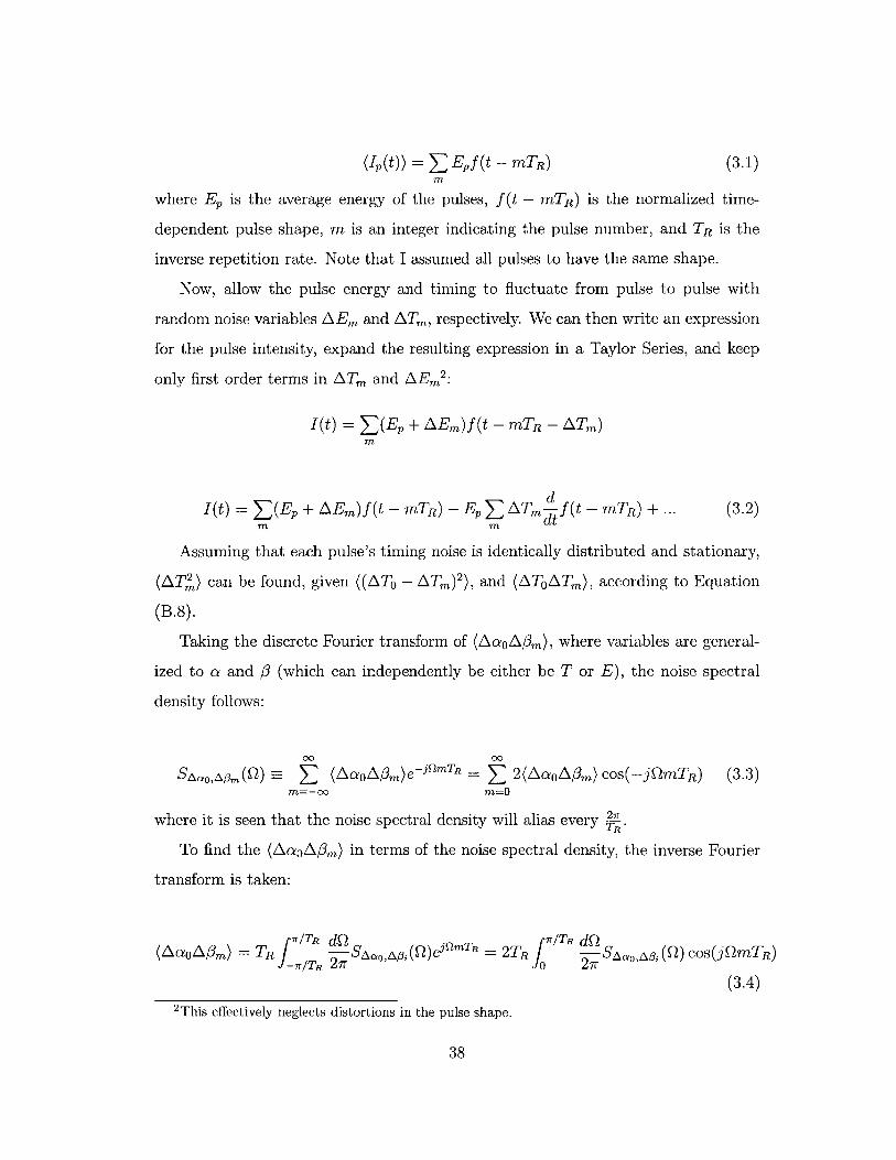
3-3 A diagram of a residual phase noise setup for laser timing jitter mea-
surem ent. . . . . . . . . . . . . . . . . . . . . . . . . . . . . . . . . . 45
3-4 A diagram of a frequency discriminator setup to measure laser timing
jitter. . . . . . . . . . . . . . . . . . . . . . . . . . . . . . . . . . . . . 47
4-1 Examples of theoretical noise spectral densities for an overdamped
(left) and underdamped (right) phase modulation [3]. . . . . . . . . . 63
13

4-2 Example of the theoretical noise spectral density for amplitude modu-
lation [3]. . . . . . . . . . . . . . . . . . . . . . . . . . . . . . . . . . 63
4-3 Example of the theoretical noise spectral density for passive modelocking. 64
5-1 Optical Correlator Setup [4]. . . . . . . . . . . . . . . . . . . . . . . . 66
5-2 Residual Phase Noise Measurement Setup used to measure the timing
noise spectral density of the Sigma Laser. . . . . . . . . . . . . . . . . 67
5-3 Sigma Laser Setup. [3] . . . . . . . . . . . . . . . . . . . . . . . . . . 68
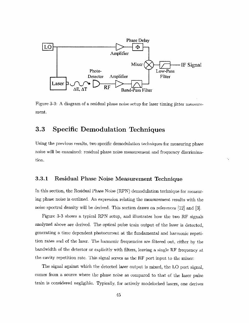
5-4 Typical optical spectrum of the sigma laser output. . . . . . . . . . . 69
5-5 Trace of the auto-correlation and cross-correlation of neighboring pulse. 70
5-6 Single Sideband measurement of the phase noise spectral density of the
sigm a laser. . . . . . . . . . . . . . . . . . . . . . . . . . . . . . . . . 71
5-7 An overlay of three noise harmonics taken using an Agilent 8565EC
RF Spectrum Analyzer (9kHz - 50GHz). The plots have been offset
slightly, to allow for better viewing. They are ordered lowest to highest
harmonic, left to right. As expected, the noise harmonics alias. ..... 72
6-1 The P-APM 10MHz laser. . . . . . . . . . . . . . . . . . . . . . . . . 76
6-2 Typical modelocked spectrum of the P-APM fiber laser. Overlayed
on this is the laser output when not in a modelocked state. One can
clearly see the filter edges coinciding with the dips in the modelocked
spectrum . . . . . . . . . . . . . . . . . . . . . . . . . . . . . . . . . . 78
6-3 Typical auto-correlation of the P-APM fiber laser. A dashed line shows
a secant hyperbolic fit to the auto-correlation trace. The bumps in the
wings of the pulse are attributed to the optical filter shape. . . . . . . 79
6-4 Digital Oscilloscope trace of a single optical pulse, and the optical pulse
train . . . . . . . . . . . . . . . . . . . . . . . . . . . . . . . . . . . . . 79
6-5 Various plots of the RF spectrum of the laser output. . . . . . . . . . 80
6-6 The frequency discriminator system used for these measurements. . . 82
14
6-7 Frequency discriminator single sideband plot of timing jitter, assuming
no correlation. Delay length is 1000m / 5.Ops (top), and 5000m /25.Ops (bottom ). . . . . . . . . . . . . . . . . . . . . . . . . . . . . . 83
6-8 Plot of the sensitivity of the frequency discriminator as a function of
frequency for various delay lengths. The first null frequency decreases
as the delay length is increased. . . . . . . . . . . . . . . . . . . . . . 85
6-9 Plot of the integration over 175kHz to 191.7kHz of SATAT-SAT(O),AT(td)
data, as a function of delay length. . . . . . . . . . . . . . . . . . . . 86
C-1 Voltage noise spectral density and sensitivity plots for 500m (2.5bts)
and 1000m (5.Ots) delay. . . . . . . . . . . . . . . . . . . . . . . . . . 104
C-2 Voltage noise spectral density and sensitivity plots for 2000m (10.0ps)
and 4000m (20.0ts) delay. . . . . . . . . . . . . . . . . . . . . . . . . 105
C-3 Voltage noise spectral density and sensitivity plots for 5000m (25.Obs)
and 6000m (30.Ops) delay. . . . . . . . . . . . . . . . . . . . . . . . . 106
15

16

List of Tables
17

18

Chapter 1
Introduction
1.1 Motivation
Considerable interest in short duration, high repetition rate optical pulse sources
exists. Many applications that require sources with these characteristics also require
low timing jitter; that is to say low uncertainty in the timing of the output pulses. The
timing jitter of pulse sources used in these applications is often a limiting factor, thus
understanding and reducing timing jitter in mode-locked lasers is of great practical
interest.
One application that requires low timing jitter is high-speed optical telecommu-
nications transmitters. Specifically, timing jitter in high-speed optical telecommuni-
cations transmitters can cause pulses to deviate from their timing "slot", leading to
bit errors, as well as further problems such as pulse interactions.
High-speed optical sampling units for analog-to-digital conversion (ADC) can also
benefit from reduced timing jitter. The current goals in effective bit resolution and
sampling frequency are beyond the performance of all-electronic ADC systems. Typ-
ical goals in effective bit resolution and sampling frequency are 12+ bits and multi-
gigahertz frequencies, respectively [1].
A promising approach is to execute some ADC processes in the optical domain
instead of the electrical domain. One can conceive of methods to both optically
sample (discretize in time) and optically quantize (discretize in magnitude) a signal.
19

ANALOG DetectionINPUT - and
Quantization
Digital.. (0,10,.Signal DIGITAL
Short-Pulse San ami Optical Processin OUTPUTOptical sampleuand -- +il qnz aSource such mp td mdCalibration eti niLinearization p l tr"a
Interleaving
mulip d n NDetectionfreq .Eahfhe l q d and -o
Quantization t
Figure 1-1: Example of an ADC that samples optically and quantizes electronically
[ll.
We will concentrate on schemes that optically sample and electronically quantize, an
example of which is shown in Figure 1-1.
In this diagram, a high-speed, short-pulse, low timing jitter optical source is fed
into a sampling transducer, such as an amplitude modulator. The electronic analog
input to be sampled drives the transducer, modulating the optical pulse train and
thus creating a pulse train where each pulse has sampled the analog signal. Because
electronic quantizers are much slower than optical samplers, the sampled signal is de-
multiplexed into N separate streams, each at a frequency of yL of the optical sampling
frequency. Each of the lower frequency demultiplexed optical streams is then fed to
an electronic quantizer. The output of each of the quantizers is then multiplexed and
signal processed, resulting in a digital sampling of the analog input.
A recent compilation of the performance of both experimental and commercial
ADC systems in terms of effective bit resolution and sampling rate is shown in Figure
1-2. One will notice the constant upper limit in resolution as a function of sampling
rate up to around 1 MHz. At sampling rates higher than I MHz, the maximum
effective bit resolution falls off by around one bit per octave. Analysis shows that
the effective bit resolution above 1MHz is limited by aperture jitter [2]. Aperture
jitter refers to the fluctuation of the time at which samples are taken. For an optical
sampling system, this aperture jitter is synonymous with timing jitter.
20

C
22
20
18
16
14
12
F slope: -1 bit/octave I - j... ........... .......... .
A AT A -*--
V m ~~hybrid 4~AhA--~+*A A
(0 ~ * 111-V ICAx SuperC
2 -state-of-the-art .. .
1E+4 1E+5 1E+6 1E+7 1E+8 IE+9 1E+10 1E+11Sample Rate (Samples/s)
Figure 1-2: Performance survey of current ADC systems [2].
System performance and the limitations timing jitter places on it can be estimated
using the following approximation [5]:
T(-7<-- (1.1)
2N
where T is the repetition rate, N is the effective bit resolution, and sigma is the timing
jitter.
Figure 1-3 expresses the same relationship. In this plot, aperture jitter is assumed
to be the only noise source. For a given sampling rate and effective bit resolution,
one can find a maximum tolerable aperture jitter. The aperture jitter performance
for modern electronic and optical sources are shown in the hatched region. One can
see that superior ADC performance can be achieved with optical sampling [1].
One should note that the aperture time also effects the performance of these
systems. Aperture time refers to the fact that sources put out pulses that are not
instantaneous, and thus the values sampled are actually a weighted average of the
analog signal over the shape of the sampling pulse. Clearly, shorter, 6 function-like
pulses are preferable. However, aperture time error is not as significant as aperture
21

10 EloctronicSampling Jitter
0.01Optiol Sampling Jitter
0.1 1 10Sampling Rate (GS/s)
Figure 1-3: Dependence of ADC performance on aperture jitter, when aperture jitter
is the only sources of noise. [1]
jitter error, and can be thought of as being included in the aperture jitter [2].
To produce the best optical sampling performance, the ideal optical source should
output high frequency pulse trains consisting of short pulses with low timing jitter.
Optical sources that hold promise for achieving these goals are semiconductor lasers,
solid state lasers., and fiber lasers. This work focuses on efforts on fiber lasers.
To create short pulses in fiber laser systems, fast saturable absorber mechanisms
such as polarization additive-pulse modelocking (P-APM) are used. Typically, the
fast saturable absorber opens a low-loss window in time, that allow the pulses to build
up in this window. The low-loss windows are created by the pulses themselves, using
nonlinear effects such as the Kerr effect. Soliton effects further narrow the pulse and
limit its duration, while filtering limits the spectrum. The final pulse width reflects
the balance of these limiting effects [6].
Generally, high repetition rates can be achieved in two ways. The first is simply to
make a short cavity. In this approach, one intracavity pulse exists in the cavity (i.e.
the cavity is fundamentally modelocked), and the length of the cavity is reduced, thus
increasing the output repetition rate. As an example, to make a 10 GHz laser in a ring
configuration, the geometric circumference of the ring will be on the order of 2 mm.
This presents problems for many artificial saturable absorber schemes that require
22

nonlinear effects to accumulate in a roundtrip. Also, fitting the necessary optical
components (bandpass filter, waveplates, isolators, etc.) into the cavity becomes
difficult.
The second approach is to increase the number of intracavity pulses in the laser;
this is known as harmonic modelocking. Harmonic modelocking circumvents many of
the problems mentioned above that one encounters in short cavity laser designs, and
shows potential for producing low timing jitter pulse trains [4].
1.2 Thesis Organization
This thesis covers two distinct sets of experiments concerned with fiber laser timing
jitter. Background for analyzing and understanding the data from these experiments
is presented in Chapter 2 through Chapter 4, which covers optical correlations, spec-
tral noise density measurements, and modelocked laser noise. Chapter 5 covers the
first set of experiments, which compare and relate two methods of measuring RMS
timing jitter. Chapter 6 covers the second set of experiments, where the timing jitter
of a 10 MHz passively modelocked P-APM fiber laser is measured using frequency
discrimination. Chapter 7 discusses final results, conclusions, and future work. Ap-
pendicies follow for reference.
23

24

Chapter 2
Optical Correlations and Timing
Jitter
This section explores the effect of timing jitter on optical correlation measurements.
Results that allow the extraction of the RMS timing jitter using optical correlation
measurement results are derived.
2.1 Optical Correlations Involving Timing Jitter
Optical correlations of two pulses are essentially a measure of the convolution of
those pulses. Typically, a pulse train is split into two paths, where the length of
one path is varied to create a relative delay between the pulse trains. The paths
are then crossed, typically inside a nonlinear crystal that generates second harmonic
frequencies (SHG) 1 . The intensity of the SHG is proportional to the overlap of the
fundamental frequency beam's intensities. The proportionality of the SHG to the
intensity of the fundamental frequency can be seen in the semi-classical equation for
SHG [8]2:
'There are methods to measure the pulse overlap other than using SHG crystals, including using
two-photon absorption in diodes or periodically-poled lithium niobate waveguides [7].2Equation (2.1) is, in general, only one of two coupled equations for sum frequency generation,
and is valid for SHG in the undepleted pump approximation. Regardless, an illustration of the
intensity dependence of SHG is all that is sought here.
25

4- Double-Arm SHGSingle- and
Double-Arm SHG minmimm+-Filter
Fundamental and SHG -
SHG Crystals --
FundamentalBeams
Non-collinear Collinear
Figure 2-1: Illustration of collinear and non-collinear optical correlator setups. The
non-collinear setup allows for easy blocking of the unwanted single-arm SHG. The
collinear geometry does not allow for this, but has other advantages, such as the
ability to make interferometric optical correlations.
dA 2 _ 47rjw 2dAleikz2 A 2 i~kz(2.1)
dz ~ k2c 2 1
where A1 is the electric field amplitude of the fundamental frequency, and A2 is the
electric field amplitude of the second harmonic frequency. The second harmonic is
measured as a function of the path delay, and the optical correlation trace is created.
All SHG photons originate from two fundamental frequency photons. These SHG
photons can be differentiated based on the origin of the fundamental photons from
which it came. "Single-arm" SHG is generated from two photons that originated
from the same beam. These SHG photons travel in the same direction as the photons
from which they originate. "Double-arm" SHG is generated by one photon from each
beam. These SHG photons travel in the direction of the average momentum of the
two incident photons, and comprise the second harmonic signal that is proportional
to the pulse overlap. For non-collinear geometries, where the two incident beam paths
do not spatially coincide, the double-arm photons of interest will be spatially separate
26

from the single-arm photons, and can thus be isolated. This results in a background
free optical correlation. Figure 2-1 illustrates this difference between collinear and
non-collinear geometries.
The "sliding" overlap integral that will comprise the correlation, will logically
look like a convolution function. An expression for the auto-correlation3 and cross-
correlation 4, respectively, where timing jitter is assumed to be absent, can be written:
Cm,m(td) - dtIm(t)Im(t - td) (2.2)
Cm,n(td) = J dtIm(t)In(t + td) (2.3)
where Cm,n (td) is the expression for the noiseless optical correlation of pulse m and
pulse n. Im(t) is the intensity of pulse m as a function of time, t. td represents the
time delay between the two pulse streams, modulo the temporal pulse spacing (i.e.
the inverse repetition rate).
At this point, noise5 must be incorporated in the auto-correlation expression.
Optical correlation data points are measured on time scales that are much longer
than the temporal pulse spacing (i.e. the inverse repetition rate). As such, the
optical correlation is the average of the correlation of successive pairs of pulses, where
each pulse's nominal timing deviation is random from pair to pair. This suggests
that the optical correlation of pulses with timing jitter will be the expectation of
the convolution, where now random delays due to timing jitter are included as an
argument of the pulse intensity function. Using the basic definition of an expectation,
an expression for the optical correlation of two pulses with non-zero timing jitter can
be written. For the auto-correlation, this is the expectation of Equation (2.2) with
timing noise added:
3The auto-correlation is the optical correlation of a pulse with an exact copy of itself.4The cross-correlation is the optical correlation of two pulses in general. The auto-correlation is
the special case where the pulses being correlated are identical.5The discussions of noise will require substantial use of probability. A review of probability
concepts are included in Section B.1 as a reference for the reader.
27

E[Cm,m(td, p(ATm, ATm))] J dAtm dtlm(t - Atm)Im(t + td - Atm) fATm (Atm)
(2.4)
where fATm (Atm) is the PDF of the noise ATm, and p(ATm, AT,) is the correlation
coefficient for the random variables ATm and AT.
Notice that this integral only depends on the relative positions in time of the
pulses; any constant time can be added to the argument of both pulses without chang-
ing the expression's result. Thus for the optical auto-correlation, since p(ATm, ATm) =
+1 always, and assuming the noise variables are identically distributed, Atm is added
to the argument of each pulse in Equation (2.4):
E[Cm,m(td, p(ATm, ATm))] = dAtm dtlm(t)Im(t + td)1 fAT.(Atm)
E[Cm,m(td, p(ATm, ATm))] = J dtIm(t)Im(t + td) (2.5)
Thus the auto-correlation does not change due to the presence of timing jitter.
An expression for the cross-correlation with noise can also be found. The cross-
correlation for two pulses, m and n, with timing jitter, results in the general expression
for an optical correlation in the presence of timing jitter:
E[Cm,n(td, p(ATm, AT))] = J dAtm J dAta
[J dtIm(t - Atm)In(t + td - Atn)1 fATm,ATn (Atm, Atn) (2.6)
where fATm,ATn (Atm, At,) is the joint PDF of ATm and AT., and the definition of
the expectation of functions of two random variables was used.
As a special case, it is seen that if pulse m and n are correlated such that
p(ATm, ATn) = +1, and ATm and ATn are identically distributed, then ATm = ATn.
We can therefore add ATm to the argument of both pulses in Equation (2.6):
E[Cm,n(td, p(ATm, ATn) =+1)] = J dAtm[J dtIn(t)Im(t + td)] fATm(Atm)
28

E[Cm,m(td, p(ATm, ATn) = +1)] = j dtIm(t)Im(t + td) (2.7)
which is equivalent to the cross-correlation without timing jitter, and becomes the
expression for the auto-correlation when m = n.
Finally, an alternate general expression for Equation (2.6) can be written. Again,
nothing is assumed about the timing jitter. By taking advantage once more of the
fact that a constant can be added to the argument of both pulses, Atm is added to
the arguments of both pulses. This results in an alternate general expression for the
optical correlation in the presence of timing jitter:
E[Cm,n(td, p(ATm, ATn))] =
j dAtM dAtn[J dtIm(t)In(t + td + Atm - Atn)] fATm,ATn(Atm, Atn)
E[Cm,n(td, p(AtM, Atn))] = j dAt[f dtIm(t)In(t + td - At)]fAT(At) (2.8)
where the definition AT = ATn - ATm is made. AT is a random variable that
describes the difference in the instantaneous timing jitter of the two pulses, and has
a PDF, fAT(At).
Note that Equation (2.6) and Equation (2.8) express the optical correlation for
two pulses, where the intensity profile of each pulse and the PDFs of the timing jitter
need only be of a well-behaved functional6 form. Each pulse and each jitter PDF
need not be the same, respectively.
6 By well-behaved, it is meant that the functional forms are such that the interpretations in the
derivation are valid. Functions that do not integrate to finite values (i.e. they are not localized) are
an example of functions that are not well-behaved. For virtually any real system, these functions
will be well-behaved.
29

2.2 Pulse Width and Timing Jitter Variance Re-
lationships
The integrals in Equation (2.6) or Equation (2.8) can only be done analytically with
PDFs and pulse shapes of a very specific form. In general, these equations require
numerical calculation. However, results can be derived that will make the numerical
work much easier that direct numerical integration. Using analogies with probability,
the pulse functions may be treated as PDFs. The pulse widths and optical correlation
trace widths may be expressed as the variance width7 . Finding the variance width
will generally require numerical calculation. The calculation results can then be used
to calculate the RMS timing jitter using algebraic expressions.
The RMS timing jitter can be easily calculated from the variance width of the
timing jitter PDF. The variance width of any function depends on the first and second
moment of that function. Only the first and second moments of the functions in the
optical correlation expression are needed to calculate the first and second moments
of the timing jitter. By working only with these moments, and not the complete
functions, the math is simplified considerably.
Beginning with the Equation (2.8) for the general optical correlation of two noisy
pulses, Im(t) and I(t) are treated as PDFs. The PDFs must integrate to unity, so
the pulse functions are written as follows:
Im(t) = Emfm(t) (2.9)
where Em is the pulse energy, and fm(t) is the pulse shape, normalized so that it's
integral is unity.
Now assume fm(t) is the PDF of a random variable, Pm. The var(Pm), or equiv-
alently, varW(Im) for the variance width of pulse m, can be found.
This substitution modifies Equation (2.8), as follows:
7The variance width, and other related notation, are defined in Section B.2.1
30

E[Cm,,(td, p(ATm, AT))]
EmEn dAt [ dtfm(t)fn(td - At + t) fAT (At) (2.10)
Notice that the integral over t of the two pulse functions resembles a convolution. If
fm(t) is symmetric, the sign of t in fm(t) can be reversed, the substitution t -+ -t
can be made, giving a form that is exactly a convolution.
When the pulse functions are treated as PDFs of Pm and Pn, this convolution
results in the PDF of Pm + Pn = AC, where AC is a new random variable, and Pm
and Pn are independent variables. Thus, the result of this integral is:
fAc(td - At) = J dt fm(t)fn(td - At - t) (2.11)
which is just the auto-correlation function. Using the probability rules for sums of
independent random variables, the variance width is simply given by:
varW(fAc) = varW(I) + varW(In) (2.12)
The equation now reads:
E[Cm,n(td, p(ATm, ATn))] =EmEn [J dAtfAc(td - At)fAT(At) (2.13)
This integral is exactly a convolution. This integral will result in the PDF of a new
random variable XC = AC + AT.
fxc(td) = j dtfAc(td - At)fAT(At) (2.14)
and its variance width is given as
varW(fxc) = varW(fAc) + var(AT) (2.15)
31

Now, AT is defined as the sum of two random variables, -ATm and AT. To
remain general, no particular correlation of these variables will be assumed. Using
Equation (B.8), the variances of these distributions can be related as follows:
varW(AT) = var(ATs) + var(ATm) - 2cov(ATm, AT,) (2.16)
Combining Equation (2.15) and Equation (2.16), the final, general result relating
the timing jitter and the auto- and cross-correlation variance widths is found:
varW(fxc) = varW(fAc)+var(AT)+var(ATm) -2 var(ATm)var(AT)p(ATm, AT,)
(2.17)
If it is assumed that the timing jitter of each pulse is identically distributed and
averages to zero, Equation (2.17) can be solved for the variance of the timing jitter,
equivalent to the square of the RMS timing jitter:
< AT2 >= var(A Tm) = varW(fxc) - varW(fAc) (2.18)2 - p(ATm, AT,)
Thus, to find the RMS timing jitter from data, only the variance widths of trace
data need be taken, the correlation of the pulse noise determined either by measure-
ment or assumption, and the values placed in Equation (2.17) or Equation (2.18), as
appropriate.
2.3 Timing Jitter Probability Density Function
The timing jitter that a pulse experiences is the result of many effects, including
quantum mechanical noise (vacuum fluctuations and spontaneous emission) added
during each pass through the amplifier, thermal noise, and acoustic noise. Often
these noise perturbations can be considered independent, and thus, via the Central
Limit Theorem, it is reasonable to expect the marginal PDF of the timing jitter of
pulse m to be well-approximated by a Gaussian:
32

A -
fATm(Atm) 1 e 2a (2.19)oAtm v'At
where the mean-squared timing jitter equals the variance (i.e. < At2 >= 02m)l-
Additionally, the timing jitter can be assumed to be stationary, thus each pulse
has the same PDF that is constant in time, the timing jitter PDF can be assumed to
be identical from pulse to pulse. As such, oatm = UAtn = oAt.
2.4 Timing Jitter Variance for Specific Pulse Forms
Specific functional forms for the pulse shapes will now be explored, and expressions
for the RMS timing jitter will be found. All pulses are assumed to be identical - pulse
shapes do not vary from pulse to pulse or with time, for times on the order of the
time it takes to complete an optical correlation. Relationships between varW and the
pulse width parameter, T, for gaussian and secant hyperbolic pulses are used. These
are given in Section B.2.3.
2.4.1 Gaussian Pulses
First, the simplest case of a gaussian pulse shape is considered. For such pulses, one
could analytically solve the integrals for the optical correlation functions, and find
the RMS timing jitter. However, the general result, Equation (2.18), is used instead.
Consider pulses that are gaussian in shape:
t2
Im(t) = Ae 2rp (2.20)
where rp is the pulse width parameter.
If the gaussian pulse shape is normalized, and treated like a PDF, the resulting
variance width is given as
varW(Im) = T (2.21)
8See Section B.1
33
Using Equation (2.18) and Equation(2.12), the RMS timing jitter is found to be:
varW (fxc) - 2-r2ATRMS var(ATm) 2arW(fxc -Tn (2.22)
\2 -p(ATm, ATE)
2.4.2 Secant Hyperbolic Pulses
The nonlinear Schrodinger Equation that describes soliton systems has solutions that
are secant hyperbolic. As such, it comes as no surprise that the pulses dealt with in
soliton fiber lasers are typically secant hyperbolic in shape.
Consider pulses with a secant hyperbolic shape:
Im(t) = Asech - (2.23)
where r is the pulse width parameter.
Using the result for the timing jitter in terms of variance widths, Equation (2.18),
and the numerical results found in Section B.2.3, the following equation for the RMS
timing jitter of two secant hyperbolic pulses is found to be:
var W(fxc) - 4.922 2ATRMS = }var( ATm) r~x)-4 (2.24)\ 2 - p(ATm, ATn)
These results will be used to calculate the timing jitter from optical correlation
data.
2.5 Optical Cross Correlation Delay Line and Dis-
persion
In practice, when doing an optical cross-correlation, achieving a large range of delays
can be difficult. A fiber delay line in one path of the optical correlator is one way to
implement this. A nice feature of this approach is the ease with which the delay length
may be changed. Group Velocity Dispersion (GVD), however, presents a problem,
as the pulses in the delayed optical fiber path will be broadened before they are
overlapped with pulses in the other path [4].
34

The error due to GVD can be calculated and accounted for, assuming higher-order
dispersion is negligible. When a dispersive fiber delay is placed in one path of the
optical correlator, it will cause pulses in that path to be dispersed when they arrive
at the nonlinear crystal. Thus, when the two pulse trains interact in the crystal, one
train of pulses will be undispersed and the other will be dispersed. This will change
varW(fAc), according to Equation (2.12). Thus, the cross-correlation measurement
can be corrected given the variance width of the dispersed pulse and the undispersed
pulse.
The dispersed and undispersed pulse variance widths can be found by making two
auto-correlation measurements, one made with no optical delays anywhere, in order
to determine the undispersed pulse width, and one made with the optical delay placed
before the pulse train is split into two paths in order to determine the dispersed pulse
width. The new expression for the RMS jitter, using a dispersive delay line is then:
< AT2 >= var(ATm)= varW(fxc) - varW(Innd) - varW(Ii.,) (2.25)2 - p(ATm, AT)
where und is the pulse shape function for the undispersed pulse, and Idisp is the pulse
shape function for the dispersed pulse.
2.6 Summary
In this chapter the mathematical treatment of optical correlations including the effects
of timing jitter was reviewed. Results relating the pulse width, via the auto- and cross-
correlation widths, to the timing jitter variance were derived. The special cases of
gaussian and secant hyperbolic pulse shapes were explored. Finally, an expression for
the variance of the timing jitter, corrected for the dispersion of a delay line used in
cross-correlations, was presented.
35

36

Chapter 3
Spectral Noise Density and Timing
Jitter
In this chapter I explore the spectral noise density expression for timing jitter, and
derive the necessary results for calculating the RMS timing jitter. I then review
specific demodulation techniques for measuring the spectral noise density.
3.1 General Derivation of the Spectral Noise Den-
sity
The timing jitter of a modelocked laser may be described and understood in the
frequency domain. In this section, expressions will be presented for the spectral noise
density function for timing jitter. The noise spectral density will be related to the
correlation function of the noise of two pulses1 . This exposition follows [9].
I start by writing the (ensemble) average intensity of an optical pulse train, (Ip(t)),
as:
'For purposes of connecting this Chapter to Chapter 2, one should note that when the expec-
tation of one of the noise variables is zero, the noise correlation function and the covariance are
interchangeable. In fact, throughout this work, it will be assumed that the expectation of the noise
variables are zero, thus this equivalence holds.
37
(Ip(t)) = EEpf(t - mTR) (3.1)
where Ep is the average energy of the pulses, f(t - mT) is the normalized time-
dependent pulse shape, m is an integer indicating the pulse number, and TR is the
inverse repetition rate. Note that I assumed all pulses to have the same shape.
Now, allow the pulse energy and timing to fluctuate from pulse to pulse with
random noise variables AEm and ATm, respectively. We can then write an expression
for the pulse intensity, expand the resulting expression in a Taylor Series, and keep
only first order terms in ATm and AEm2 :
I(t) = (Ep + AEm)f(t - mTR - ATm)m
I(t) = Z(Ep + AEm)f(t - mTR) - Ep ATmd f(t - mTR) + ... (3.2)
Assuming that each pulse's timing noise is identically distributed and stationary,
(ATm2) can be found, given ((ATo - ATm) 2 ), and (ATOATm), according to Equation
(B.8).
Taking the discrete Fourier transform of (AaoAi3m), where variables are general-
ized to a and 0 (which can independently be either be T or E), the noise spectral
density follows:
00 010
SAaO,Am(Q) E (ACeOOm)e6 j1MTR = R 2(AaoA3m) cos(-jQmT) (3.3)m=-o m=O
where it is seen that the noise spectral density will alias every q.
To find the (AaoAQm) in terms of the noise spectral density, the inverse Fourier
transform is taken:
/T dQ f/TR dQ(AOZA3m) = TR] 'SaOAfT(Q eijmTR = 2TR (SQ0 ApiQ) cos( jQmTR)
-W/TR 2r Jo 27r(3.4)
2This effectively neglects distortions in the pulse shape.
38

where one should note that integral should only be over "one alias" of the spectral
noise density.
Using these expressions, the mean-squared timing jitter between two pulses, given
the timing jitter spectral density, is:
2/A T2 Tf' df
(AT = - SATO,"N T() (3.5)- irITR 27
where the expectation of the timing jitter is taken to be zero. Using this expression,
the RMS timing jitter is calculated from the timing jitter spectral density.
3.2 General Demodulation Measurement
Two ways3 to measure the timing jitter of a modelocked laser are direct detection
and demodulation. In direct detection, proposed by von der Linde [11], the laser
output intensity is detected. The amplitude noise and timing jitter of the laser output
produces noise in the generated photocurrent. This photocurrent is then viewed on
an RF signal analyzer, where the amplitude and timing jitter appear as sidebands
about the carrier. By looking at several harmonics, one can estimate the timing
jitter value, using the fact that sidebands due to timing jitter go as the square of the
harmonic number, and the amplitude sidebands are constant. While this method is
simple and quick, quantitative results are fairly inaccurate. Much better quantitative
results may be obtained using a demodulation technique.
A general demodulation scheme mixes two signals, both of which may contain
noise. The mixing products are a baseband set of the noise sidebands with the carrier
removed, and a second harmonic signal with noise sidebands. The second harmonic
is filtered out, and the baseband noise is observed.
Demodulation has several advantages over direct detection. Direct detection the
carrier consumes more of the RF spectrum analyzer's dynamic range, whereas demod-
ulation removes the carrier at baseband, allowing one to view the sidebands using the
full dynamic range. Thus one can observe much greater detail in the noise spectrum3 Other methods may be used, such as Phase-Encoded Optical Sampling [10].
39

LO Phase Delay
AE, AT Amplifier
Mixer - IF SignalLow-Pass
RF Amplifier Filter
AE, AT
Figure 3-1: Example of a general demodulation scheme for amplitude and timing
noise measurement.
and extract more accurate quantitative results. Also, demodulation allows one to
bias the measurement system to either suppress amplitude noise or the timing noise,
as will be described.
Figure 3-1 illustrates a general demodulation scheme. Two RF signals of the same
frequency, both containing amplitude and phase noise, are amplified to appropriate
levels, are adjusted in relative phase, and are combined in a mixer. The second
harmonic frequency generated by the mixing is filtered with a low-pass filter, and the
resulting mixing products are the noise sidebands at baseband.
Note that nothing was said thus far about the origin of the RF signals. The origin
of the RF signals is specific to the measurement scheme, and will be covered in Section
3.3.
In this section, the demodulation of two signals with amplitude and timing noise
will be derived. Subsequently, two specific demodulation measurements will be ex-
amined.
3.2.1 Mixing Products
I begin with the expressions for the time-dependent voltages that are the RF and LO
inputs of the mixer. They can be written as:
40

VRF(t) = (VRF + AVRF(t - td)) sin (21rfo (t - td) + ADRF (t - td))
VLo(t) = (VLO + AVLo(t)) cos (27rfot + A4LO(t)) (3.7)
where V are the voltage amplitudes with i = RF, LO; fo is the nominal frequency of
the signals; td accounts for any time delay between the RF and LO signals; and AV(t)
and A'i(t) are the random variables for the voltage amplitude noise and phase noise,
respectively.
Notice that Equation (3.6) and Equation (3.7) are written to be in quadrature
when the phase adjustments due to the phase noise variables and delay are the same
for both input signals. By mixing the signals in quadrature, the voltage output of the
mixers is biased to be most sensitive to phase noise and to suppress the amplitude
noise. Figure 3-2 illustrates this. With quadrature biasing, the zero crossing of the
LO sinusoid is aligned with the peak of the RF sinusoid. Amplitude fluctuations in
the RF signal, being multiplied by the small amplitude of the LO signal in the mixer,
are damped out. Phase deviations in the RF sinusoid, however, are multiplied by the
peak of the LO signal, resulting in large changes in the mixer output.
To maintain quadrature, it is clear that the time delay in the RF port signal must
be discrete such that:
t Pd (3.8)2 fo
where Pd = 0, 1, 2.... The mixing products of Equation (3.6) and Equation (3.7), after
a little algebra, are given as:
AV(t) = a(VRF + AVRF(t - s)) (vLO +AVLO(t))
sin (27r(2fo)t - Pd7 + A'IRF(t - Ld ) + ALot))
+ sin (A4RF(t - )d - A'LO(t) - Pd7r) (3.9)
41
(3.6)

Temporal Overlayof LO and RF Signals
in Quadrature
MixingProducts
DC Componentof Mixing Products
A<D
AE
/7
Figure 3-2: An illustration of how quadrature mixing makes the detection system
sensitive to phase fluctuations and insensitive to amplitude fluctuations. Fluctuating
signals are shown as dashed lines.
where a is the mixing coefficient. The DC and second harmonic results appear clearly.
The low-pass filter next strips out the second harmonic component, giving:
AV(t)cPd P A= kyVRFVLO + AVRF(t - )VLO + VRFAVLO(t) + AVRF(t - Pd)VLO2 2f 2 fo
sin (AJRF(t - Pd A (3.10)2fo
where the sign in front is positive for even Pd and negative for odd Pd.
At this point, all amplitude noise terms are second order or higher. Taking the
noise variables to be small, all second and higher order terms are ignored:
AV(t) = k aVRFVLO sin A RF(t - Pd) - A 'LO(t)2 2 fo
AV(t) = ±Ko sin A4RF ( - P A2f LOM
where Ko = VRFVLO
(3-11)
42

Assuming that the phase deviations are small compared to a radian, /MN << 1,
sin(x) can be approximated as x, resulting in:
AV(t) ~ ±K, (ARF(t ~ Pd APdLO(t) (3.12)2 fo LO,
Finally, the mean-squared values of Equation (3.12) are found, Equation (3.4) is
substituted in, and common integrals and factors are removed, resulting in the phase
noise spectral density expression:
SAvAv (fm) = K2 (SAm RF,ADRFfM) + SAILOAILO fM) -2 SADRFALO (fm) Cos(QMTR
(3.13)
3.2.2 Phase Noise and Timing Jitter
The phase noise quantities, Abi, can be written in terms of the timing jitter quanti-
ties, AT. This can be simply done using:
A5i(t) = 27rfoAT(t) (3.14)
where i = LO, RF. By taking the mean-squared value of this equation, using Equa-
tion (3.4), and removing the common integrals and factors, the timing noise and phase
noise spectral densities can be related:
SAciA4(fm) = (27rfo) 2 SAT,AT(fm) (3.15)
The mixing products can then be cast in terms of the timing noise variables:
AV(t) ~27rfoK, ATRF(t - d- ATLO(t) (3.16)
sv,v (fm) = (2,rfoKO)2 ( SATRF,ATRF (fin) + SATLO,ATLO (i)
-2
SATRF,ATLO fM) COS(QmTR)) (3.17)
43

3.2.3 Single Sideband Noise and Phase Noise Spectral Den-
sity Relationship
The conventional way to express the phase noise of a signal is to display the single
sideband (SSB) noise, L(f m ). This is often taken to be a plot of the noise sidebands
that are generated when the carrier is modulated with the noise spectral density, nor-
malized by the total signal power. Assuming that the noise power is small compared
to the signal power, L(f m ) is often approximated as the SSB plot normalized by the
carrier power alone. The units of L(fm) are dBc/Hz, the power normalized to the
carrier power in a 1 Hz bandwidth at fm offset frequency from the carrier.
For each specific demodulation measurement technique, a relationship between
L (f m ) and the phase noise spectral density, SAAp (fm), is desirable. This relationship
will be established. Again, the assumption that the noise power is small compared to
the carrier power is used. When a carrier is phase modulated, sidebands are generated,
and their magnitudes are Bessel functions of the peak phase deviation of modulation,
J, (O), where 3 is the peak phase deviation. If the phase deviations are taken to be
small enough, the Bessel functions can be approximated as 3, and the mean-squared
phase deviations become . Looking at the ratio of the single sideband power to the
carrier power, L(f m ), 02 is arrived at, giving:
L(f m ) = SA-b,A.(fm) (3.18)2
This expression can be rewritten in terms of the timing noise spectral density,
using Equation(3.14):
L(f m ) = 2(7rfo) 2 SAT,AT(fm) (3.19)
The reader is referred to [12] and [13] for more details.
44
Phase Delay
LO >- DAmplifler
Mixer - IF SignalPhoto- Low-Pass
Detector Amplifier Filter
AE, AT RE Band-Pass Filter
Figure 3-3: A diagram of a residual phase noise setup for laser timing jitter measure-
ment.
3.3 Specific Demodulation Techniques
Using the previous results, two specific demodulation techniques for measuring phase
noise will be examined: residual phase noise measurement and frequency discrimina-
tion.
3.3.1 Residual Phase Noise Measurement Technique
In this section, the Residual Phase Noise (RPN) demodulation technique for measur-
ing phase noise is outlined. An expression relating the measurement results with the
noise spectral density will be derived. This section draws on references [12] and [3].
Figure 3-3 shows a typical RPN setup, and illustrates how the two RF signals
analyzed above are derived. The optical pulse train output of the laser is detected,
generating a time dependent photocurrent at the fundamental and harmonic repeti-
tion rates and of the laser. The harmonic frequencies are filtered out, either by the
bandwidth of the detector or explicitly with filters, leaving a single RF frequency at
the cavity repetition rate. This signal serves as the RF port input to the mixer:
The signal against which the detected laser output is mixed, the LO port signal,
comes from a source where the phase noise as compared to that of the laser pulse
train is considered negligible. Typically, for actively modelocked lasers, one derives
45

the reference signal from the local oscillator that is driving the modelocking element
in the laser.
As stated, this technique assumes that the phase noise of the reference signal is
negligible, i.e. A4LO = 0, compared to that of the laser system under test. In essence,
the LO signal is assumed to be a perfect sinusoid. Starting off with Equation (3.11),
these assumptions are used, giving:
AV(t)~ KOA(DRF(t)
The resulting voltage is linearly proportional to the phase deviations created by the
timing jitter. Note that A4(t) is a random quantity, and thus AV(t) will also be
random. However, for constant phase delays the above equations are still valid, which
gives a way to measure KI, as will be seen in Section 6.1.3.
This expression is solved for the phase noise variable, and then rewritten in terms
of the timing jitter, using Equation (3.14):
ADRF(t) fAV(t) (3.20)KO
ATRF (t) eAV(t) (3.21)27rfoKo
Using Equation (3.4), the phase noise spectral density, SA(RFA4RF (i) , can easily
be written as a function of the voltage noise spectral density, SAvAv(fm). To do this,
the mean-squared values of both sides of the Equation (3.20) are taken, are written
as integrals of the spectral noise densities, and common integrals are removed:
SA(RF,A4RF UM) K f2 (3.22)
which, doing the same for Equation (3.21), the analogous expression for the timing
noise spectral density is found:
SATRF,,TRF UM) 1_0 fzKi(fM) (3.23)(2irfoK ) 2
Finally, using Equation (3.18), the single sideband expression for RPN is derived:
46

Fiber Delay AE, AT LO Band-Pass Filter
Photo- Amplifier (D Phase DelayDetector
Laser 3dB Mixer IF Signal
Couplet Photo- Low-PassCouplet Detector Amplifier Filter
AE, AT RF Band-Pass Filter
Figure 3-4: A diagram of a frequency discriminator setup to measure laser timing
jitter.
SAVV( fm ()LRPN(fm 2K2 (3.24)
3.3.2 Frequency Discriminator Technique
In this section, the Frequency Discrimination (FD) demodulation technique for mea-
suring phase noise is outlined. An expression relating the measurement results with
the noise spectral density will be derived. This section draws on references [12] and
[13].
Figure 3-4 shows a typical FD setup, and illustrates the origins of the RF and LO
signals. The optical pulse train is split into two essentially identical pulse trains. One
pulse train is detected and filtered leaving one harmonic, at frequency fo as given in
Equation (3.7), of the detected signal - this serves as the LO signal. The other pulse
train is delayed by some amount of time, td = P, according to Equation (3.8), is
then detected, and filtered for one harmonic - this serves as the RF signal. Again,
the timing noise of the pulse trains manifest as phase noise in the detected sinusoidal
signal, and amplitude fluctuations appear.
The general results of Equation (3.12) and Equation (3.13) are easily specified to
this case. The phase noise variables for both the RF and LO signal as a function of
time are clearly the same, as they originate from the same pulse train, thus A<DRF(t) ~
47

A~Lo(t) = A4(t). This gives:
AV(t) ±K, A(D(t - )fo A1(t) (3.25)
SA VAV UM) Pd (.6SA1(t),'A(t)(fm) ~ K ) + SAD(t)',(t-_ Pd fm) COS j27rfm (3.26)
Using Equation (3.14), these two expressions can be written in terms of the timing
noise:
AV(t) ±27rfoKo ATRF(t - Pf - ATLO(t) (3.27)
SAVAV(fm) e PdSAT(t),AT(t) (fM) 2(27K)2+ SATt),ATt_ y() (3.28)
and from these the single sideband measurement is found using Equation (3.18):
L(fm) = SAV2NYM) + 2(7rfo) 2 SAT(t),T(t-d) cos 27rfm (3.29)
where the noise spectral densities are for positive frequencies. Notice that the mea-
surement is of SAy(fin), and an assumption must be made about the correlation of
the noise variables.
Sensitivity
The phase modulation of a signal can also be described as a frequency modulation.
A signal that undergoes a frequency change will have, after propagating a distance,
a resulting phase change as compared to the phase of the signal at the end of the
propagation distance before the frequency change occurred. In this way, the delay
line converts the frequency deviations associated with the timing jitter into phase
deviations proportional to the delay length at the mixer. By analyzing the frequency
48

discriminator in terms of frequency noise, the frequency discriminator sensitivity can
be derived.
The relationship between the phase, timing, and frequency must first be estab-
lished.
Of = (3.30)27r at
The Fourier decomposition of the phase fluctuations can be written and compared to
the Fourier decomposition of the frequency fluctuations in order to write the Fourier
amplitudes of the phase fluctuations in terms of the Fourier amplitudes of the fre-
quency fluctuations. For a particular frequency of phase modulation, fn, the phase
variable can be written as:
A4D(t, fm) = A(bo(fm) sin(27rfmt) (3.31)
where AdIo(fm) is the amplitude of the Fourier component of the phase deviations
at fm. Using Equation (3.30), the fm component of the corresponding frequency
modulation, AF(t, fm), can be found:
AF(t, fm) = A4bo(fm)fm cos(27rfmt) (3.32)
Thus, the amplitude of the Fourier component of the frequency modulation, call it
AFo(fm), is given as:
AFo(fm) = A o(fm) fm (3.33)
Solving for A<Do(fm), Equation (3.31) can be substituted:
AFo(fm)A4D(t, fm) = sin(27rfmt) (3.34)
fin
Notice that the integrals of Equation (3.31) and Equation (3.32) over (positive) fm
result in the time dependent phase and frequency changes, respectively.
Equation (3.34) is substituted in for the noise variables in Equation (3.25) resulting
in the output voltage as a function of time and modulation frequency:
49

rVt fA Fo(fm) P A Fo (fm)AV(t, fm) iKO f sin(27fmt - 7rfm-) - f si(27rft))
AV(t, fm) ~ ±Ko2AFo(fm) sin(7rfm Pd )cos(27rfmt - Prfm ) (3.35)fm 2fo 2fo
The cosine term describes the time dependent output of the mixer. The coeffi-
cient of this cosine, KFD, describes the sensitivity of the system. This coefficient is
rewritten as:
pasin(7r fm 2KFD = iK27rAFo(fm)2 P rf ") (3.36)
The sensitivity has a si7x) dependence, with nulls at:
= 1 2fo (337)m,nu (3td Pd
Around these nulls, the sensitivity is extremely poor.
Ideally, the frequencies of interest will be well below the first null. A generally
accepted criterion is that, if the maximum frequency of interest, fmax, is such that:
fmax < = f (3.38)2 7rtd 7rPd
then the sensitivity can be taken as constant.
For frequencies closer to the null, a correction for the sin(x) dependence can be
incorporated. However, it must be realized that the sensitivity still degrades closer to
the null, and measurements are virtually useless at the null. The generally accepted
criterion for valid measurements using a correction for the !") dependence is:X
fmax < - fo (3.39)2 td Pd
Looking back at Equation (3.36), it can be seen that, to improve the sensitivity, the
value of the time delay can be increased, via Pd. While this increases the sensitivity,
50

it decreases the first null frequency, and increasingly limits the range of frequencies
at which measurements can be effectively made.
One must also account for, when increasing the delay time, the loss of the delay
line. This loss will reduce VRF, and thus reduce K0. This leads to the existence of
an optimal delay length for a particular range of frequencies. For microwave systems,
this issue has practical significance. Due to the extremely low loss of optical fiber
delay lines, on the order of 0.2 dB/km, however, it is much less of an issue of concern.
Choice of Harmonic Frequency for Phase Detection
One feature of the derived results that should be explored regards the frequency, fo,
that is filtered out and used after the optical pulse train is detected. For a laser
system at repetition rate ffnd, the fundamental frequency need not be chosen; any
higher harmonic in which there is sufficient power can be used. To account for this
possibility, the fundamental frequency is rewritten as:
fo = Nffnd (3.40)
where N is the harmonic number of the harmonic that is chosen.
Unfortunately, it turns out that the change of variables from A1b to AT brings
a factor of 27rNffnd according to Equation (3.14), and the relationship between fre-
quency and timing incurs a factor of 2rNf according to Equation (3.30), resulting
in the same sensitivity to timing fluctuations. Equation (3.40) is used to rewrite
Equation (3.36) as:
sin(7rf, PdKFD = kK07r2AFo Pd (2ffld) (3.41)
2Nff,,d 7~rn ,,P2Nff nd
Changing the chosen harmonic, in effect, has the same effect on the sensitivity as
changing the delay length.
Changing the harmonic has other implications. In looking at the assumptions
made in deriving these results, it is seen that by increasing the operation frequency,
the assumption that the phase noise is much less than one radian becomes more
51

restrictive. Higher harmonics can be used to increase the sensitivity and reduce the
need for long delay lines, but only to the extent that the phase noise is still less than
one radian at the harmonic frequency.
The Delay Line
The delay line, as shown, has a significant impact on the operation of the frequency
discriminator. As such, there are other issues of practical nature regarding the delay
line that should be considered and addressed.
The first issues concerns the effect of thermal variations on the delay line. Ther-
mal variation will effect both the physical length of the delay line, and the index of
refraction. The latter effect on the index of refraction is much more significant, so
physical length variations will be ignored in this discussion.
Typically, the thermal dependence of the index of refraction on temperature is
on the order of nT 10-9. The time delay of the delay line is given, in terms of
refractive index, n, and physical length, Ld, as:
td = nLd (3.42)C
where c is the speed of light. Thus, for temperature variation, AT, the delay time
variation is:
nT AT LdAtd(AT) = (3.43)
These thermal variation will need to be small enough that quadrature is not deviated
from significantly.
The thermal time delay variations can be rewritten as thermal phase variations in
the detected signal. Using Equation (3.14) of the detected signal, the thermal phase
variations are found:
Aqpd(AT) = 2 7rNffndnTATLd (3.44)C
52

As the harmonic frequency of operation is increased, the thermal phase deviation for
given temperature change is increased. This means that higher operating frequencies
will be more susceptible to thermal variations in the delay line - the delay line becomes
more sensitive to both signal variations and thermal variations.
The second question regards the effect that the dispersion in the optical delay line
will have on the measurement. Fortunately, the pulse broadening due to dispersion
will have no effect on the measurement. The optical pulse train can be written as
the sum of Fourier components that comprise the combined RF and optical spectrum
of the pulse. Because the detection and filtering only leave a single frequency of the
Fourier composition of the pulse train, the dependence of the propagation constant
on frequency.
3.4 Summary
In this Chapter, a frequency-domain picture of phase (timing) noise was developed.
General demodulation techniques for measuring phase noise were then reviewed. Two
specific techniques, residual phase noise and frequency discrimination, were reviewed
in detail, sensitivities were derived, and other considerations were discussed.
53

54

Chapter 4
Modelocked Laser Noise
4.1 Soliton Theory
In this section, relevant results of soliton theory are briefly summarized. This section
follows [14].
The existence of optical soliton solutions in waveguides was first predicted by
Hasagawa and Tappert [15]. The Nonlinear Schrodinger Equation is the fundamental
equation that governs the formation of solitons, and is given as:
da F1 d2
j = 1"d2 + 11a12 a (4.1)
where a is the field, /" is the group velocity dispersion (GVD) 1 , and q is the nonlinear
Kerr coefficient. In cases of anomalous dispersion (0" < 0), solutions to the NLSE
exist, and these are solitons.
The fundamental soliton solution 2 is of the form:
a(z, t) = Psech(!)ej'!2 (4.2)
where T is the pulse width, and Ps, related to the peak power of the soliton, is given
by:
'See Section A.12The fundamental, or N = 1 solution, is the only solution of concern to us, as higher order soliton
solutions are unstable.
55

PS = 2 (4.3)r/Tr
As such, a relationship between the pulse width and peak power, or energy, is set
by the system parameters, the dispersion and nonlinear coefficient. This relationship
is called the Area Theorem:
E, = 2PT (4.4)TT
where E, is the pulse energy.
4.2 The Master Equation
In a soliton laser, effects such as gain, loss, spectral filtering, noise, and active mod-
ulation effect the development of the soliton. These effects result in the addition of
terms to the NLSE. In addition, the Kerr nonlinearity can, in general, lead to self-
phase modulation (SPM) and/or self-amplitude modulation (SAM). Thus, the Kerr
nonlinearity term is rewritten where SAM and SPM are separated.
It is also convenient to cast the NLSE in terms of two timescales, t and T. The
first time scale, t, is on the order of the pulse duration. The second timescale, T, is
on the order of a cavity roundtrip, TR. Making this change, the NLSE is modified
and recast as the Master Equation:
d [Q2TR da - D at2 + Q 6) a|2 a =
,1,82 MAM _- jMPM CSg - 1 2 (1- cos mt)1 a + TRS (t, T) (4.5)Q2 at 2 2
where the parameter, D, now expresses the average dispersion in one roundtrip of
length d.3 The Kerr coefficient, rj, has been replaced with -y - j6, where Y is the
effective SAM coefficient and 6 is the effective SPM coefficient. Both are averages
3Here, D = .1"d. This is different than the alternate notation for dispersion, given in Appendix
A.1.
56

over a roundtrip, and thus are proportional to rd. The spectral filtering is expressed
by the filter bandwidth, Qf, where the filter shape was Taylor expanded about the
peak transmission and includes only terms to second order. The active amplitude
and phase modulation depths are expressed by MAM and MPM, respectively, where
wm is the modulation frequency.4 Finally, the stochastic variable, S(t, T) drives the
noise in the laser. General analytic solutions for this equation have not been found.
One should be careful when comparing the notation here with that of Chapter
3. The driving noise term, S(t, T) is not the representation of the noise spectral
densities, Si (fin). Section 4.3.4 provides information that will further clarify the
notation.
It is clear that solutions to the Master Equation are not strictly solitons. However,
assuming that the effects that were added to the NLSE to arrive at the Master
Equation are small per roundtrip, it is reasonable to think that solution to the Master
Equation are soliton-like solutions, or solitary pulses.
4.3 Soliton Perturbation Theory
The noise term in Equation (4.5) will be treated in this section. The noise is handled
using perturbation theory; as such, the noise perturbation to the NLSE must be
assumed small. This section draws on [3] [4] [16].
4.3.1 Linear Perturbation of NLSE Solution and Equation
One starts by writing our solution as the solution to the NLSE, modified by a small
linear perturbation:
{ 2Ta(t, T) = [a.(t) + Aa(t, T)] e- o (4.6)
where a,(t, T) is the soliton solution to the NLSE using the notation of the Master
Equation as given here:
4 It was assumed that the active amplitude and phase modulation are in phase at the same
frequency. Such a situation would occur using a dual-drive amplitude-phase modulator.
57

ao(t, T) = Aosech ( exp A T(4.7)
and thus:
a,(t) = Aosech ( (4.8)
The linearly expanded solution to the NLSE is substituted into the Master Equa-
tion, and terms beyond first order in Aa(t, T) are ignored. More information on this
substitution can be found in [16]. The resulting equation will be used to project out
the equations of motion for the pulse parameters.
4.3.2 Expansion of Linear Perturbation in Pulse Parameters
One expands the perturbation, Aa(t, T), to first order in a Taylor Series about the
exact soliton solution in the four pulse parameters: energy, phase, frequency, and
timing:
0a8 (t) Oa(t) ____)
Aa(t, T) = |W=WO(w(T) - wo) + | Ioo0 (0(T) - Oo) + |a(t) =PO(p(T) - po)
+at It=to(t(T) - to) + ac(t, T)
Aa(t, T) = fw(t)Aw(T) + fo(t)AO(T) + fp(t)Ap(T) + ft(t)At(T) + ac(t, T) (4.9)
where Ai are the noise variables of the respective pulse parameter, and ac(t, T) is the
coupling of the pulse to the continuum.
One can then find the equations of fi(t, T) functions:
fw(t, T) = I - Atanh (A) a8 (t) (4.10)
fo(t, T) = ja,(t) (4.11)
ft(t, T) = -tanh (t) a.(t) (4.12)
2fp(t, T) = j-ta(t) (4.13)
WO
58

One would like to project a particular noise variable out of the Master Equation
to arrive at the equation of motion for that variable. To do this, an orthogonal set of
adjoint functions is defined:
f-w(t, T) = 2a,(t) (4.14)1 -
f..o(t, T) = 2j- [I - -tanh (t)] a,(t) (4.15)
f-t(t, T) = -ta 8 (t) (4.16)
f-p(t,T) = j ( 2 tanh (- a,(t) (4.17)(WOT 7
where, by orthogonality:
- Re [Jdt'f* (t')fj (t') =6, (4.18)
4.3.3 Projecting Out The Noise Variable Equations of Mo-
tion
Equation (4.9) can be substituted into the linearly perturbed Master Equation. The
orthogonality of the functions and adjoint functions can then be used to project the
pulse parameter noise variables. Doing so leads to the following equations of motion
(as a function of T) for the projected noise variables:
TR-Aw [-2g8s + 2-yA] ± T RSw(T) (4.19)OT
TRT AO = -6A Aw +TRSo(T) (4.20)OT 0W
T aR-T = g Ap + MPMWAT ± TRSp(T) (4.21)TROT AP 3 2T2 A PW
2 ' 2MAM22TR AT = -2DIAp - 2 WmT 2AT+ TRSt(T) (4.22)
where g. is the saturated gain, and is defined in terms of other pulse and system
parameters. The reader is referred to [16] for details of the manipulation.
59

In the context of this work, Equation (4.22) and the coupling of the other pulse
parameter noise variables is of interest.
4.3.4 Deriving the Noise Spectral Density Equations
Using the equations of motion, the noise spectral density equations in terms of the
noise source variables, Si(T), can be derived. This is most conveniently done in the
frequency domain. Thus the following Fourier Transform pair is used:
f( f(T)e~50T dQ (4.23)
f (T) = f (Q)eilTdT (4.24)
where Q is the angular frequency variable, and the factor of To in front is a normal-
ization time that prevents divergence of the spectrum.
The noise spectral densities in this Chapter will be written as ( IAi(Q) 2), where
Ai is the noise variable. Given the To factors that appear in the Fourier Transform
pairs, (IAi(Q)12 ) is the noise spectral density. This change of notation is done to
remain consistent with the source literature.
Specific cases can now be observed, and the equations for the timing noise spectral
densities can be derived.
4.4 Specific Cases of the Master Equation
The terms that appear in the Master Equation, Equation (4.5), will vary depending
on the nature of the system being described. In the following sections active and
passive modelocking equations are briefly reviewed, and expressions for the timing
noise spectral densities are found.
60

4.4.1 Active Modelocking
For an actively modelocked soliton laser with amplitude and phase modulation, the
Master Equation becomes:
D 2 _j a1- JDo2 -iSo~aI
+ TRS (t, T)Ia+ Eg
- 1 +1 92 MAM - jMPM -COSWmt)1 a
2 (.2)
(4.25)
where the SAM coefficient is set to zero. The resulting equations of motion are:
aTR a w
aT
TR-a POT
TRa AT5T
S-2gsAw + TRSw(T)
= -6AO + TRSo(T)wo
4 g_2A+ RpT3 Q2 g2 AP + MPMWZT+TRS(T)
= 2 MAM 2 2-- 2IDIAp - 2 WrMT AT+±TRSt (T)
(4.26)
(4.27)
(4.28)
(4.29)
Transforming to the frequency domain, solving for the mean-squared spectrum of
the timing noise, and ignoring cross-coupling terms, one finds the expression for the
noise spectral density for active modulation:
(IAT( )12)(jSP(Q) 2) 42 + (I(Q)12)
~fQ) ( ±P2 ) +QPM
where the following parameters are defined as:
QPM 2ID|MPMw 2
1 7 r2 MAM 221TAM 3 2 TR
1 4 1
Tr 3Q2r 2 T
61
ddT
+Q2)
(4.30)+ 2Q2M(AT -Q2 )
(4.31)
(4.32)
(4.33)

Figure 4-1 and Figure 4-2 shows three plots of the phase noise spectrum using
realistic values for the equation parameters. One plot is of the phase noise spectrum
with pure amplitude modulation (QPM = 0) and the other two are with pure phase
modulation (rAM --+ oo).
4.4.2 Passive Modelocking
In the case of a passively modelocked laser, the Master Equation will take on the
following form:
d a2 1 1921TR-a = [D + ( - -3)la a + -1+ a + TRS (t, T) (4.34)
where effective values for -y, and 6 will be specific to the passive modelocking mech-
anism. All active modulation depth parameters have been set to zero. The resulting
equations of motion are:
aTRa Aw = [-2g, + 2-yA2]Aw + TRSW(T) (4.35)
OT
TRaAO = -6A2AW +TRSo(T) (4-36)aT 0WO
TRaT Ap = 4 2 Ap + TRS(T ) (4.37)aT 3 Q 2 2
aT
Solving for the mean-squared spectrum of the timing noise, and ignoring cross-
coupling terms, one finds:
I 41D 12 (1 S (Q) 12) _ IS Q 2
(IAT(Q))2 T +2 +(St(2)I2) (4.39)
Notice the 1 dependence. Because there are no damping terms in the equation of
motion for the timing noise, as expected, the timing jitter experiences a random walk.
Figure 4-3 shows a plot of this spectrum in which realistic values for the parameters
were used. Experimental analysis in Chapter 6 will make use of Equation (4.39) that
generated this plot.
62

0.
-10-
-20-30--40 . . -........................... ....... . . ..............
-60-70.
-80-90' .. .....
-100
E
C)
E
0
z IM 1
E
C
-
E
-o-
0M 0
10.0 . -........ .... .........
-10--20-
-30- . ...
-40 -.. . . ... .................. . . .... _ _
-50
-60--70 ..- -........ ... ....... ........ ----80190'
10 100 1k 10k 100k
Offset Frequency (Hz)IM 10M
Figure 4-1: Examples of theoretical noise spectral densities for an overdamped (left)
and underdamped (right) phase modulation [3].
0
z
'U.
010- ..... .
-20 --- . . ........... ..... .
-30- ...... --.. --
-40- . . ... ..............-.
-60
-70-. .... _ __ _ _ _ _ __
-80-90-
10 100 1k 10k 100k
Offset Frequency Hz
I M 10M
Figure 4-2: Example of the theoretical noise spectral density for amplitude modula-
tion [3].
63
100 1k 10k 100k
Offset Frequency (Hz)
10-110 . .. . . . . . - . . . . . . . .

4)
z
20U
20
-
-40
-60 - - .... ...........
.120
10 100 1k 10k 100k
Frequency (Hz)IM 10M
Figure 4-3: Example of the theoretical noise spectral density for passive modelocking.
4.5 Summary
In this chapter, soliton theory was briefly reviewed. The Master Equation and it's
solutions were discussed, and perturbation theory was used to treat noise. From this,
equations of motion for the mean-squared noise variables were derived. The cases of
active and passive modulation were then explored.
64

Chapter 5
Experiments Comparing Optical
Correlation and Spectral Density
Timing Jitter Measurements
The first set of experiments performed compares the measurement of the timing jitter
of an harmonically modelocked fiber laser using two techniques. One technique uses
optical correlations and the fact that the timing jitter effects the cross-correlation
width but not the auto-correlation width. The other technique, the residual phase
noise technique (RPN), beats in quadrature the detected RF harmonics against a
"noiseless" reference signal at the same frequency, and examines the spectrum of the
resulting baseband.
5.1 Experimental Setup
I set out to demonstrate experimentally that either a set of optical correlation mea-
surements or a set of noise spectral density measurements would give equivalent re-
sults for the RMS timing jitter. This work was done in collaboration with Matthew E.
Grein. This section describes the details of the experiments as they were completed.
65

TranslationSpeaker Stage
Fiber lelay
V4 Chopper
Polarizer
Crystal
A PhotomultiplierInput
Tube
Figure 5-1: Optical Correlator Setup [4].
5.1.1 Optical Correlation Measurement Setup
For the optical correlation measurement, a non-collinear optical correlator with a
nonlinear second-harmonic generating POM crystal was used. Figure 5-1 illustrates
the design. The delay of one arm is implemented with a motorized translation stage,
which is scanned during a correlation. The correlator was built with the option to
use a fiber delay to create long delays. In these measurements, the fiber delay was
not used. This system was built by Leaf A. Jiang.
5.1.2 Spectral Noise Density Measurement Setup
A residual phase noise measurement system was used to measure the phase noise spec-
tral density. This system is shown in Figure 5-2. The optical pulse train is detected
using a Discovery Semiconductor photodiode (Model DSC40S, 16 GHz bandwidth).
This signal is amplified with a JSA Technologies Amplifier (Model: JCA812-600,
66

Phase Delay
Amplifier
Mixer IF Sig-nalPhoto-
Detector Amplifier
Laser D -R.FAE,AT RF
Figure 5-2: Residual Phase Noise Measurement Setup used to measure the timing
noise spectral density of the Sigma Laser.
+60dB gain) and beat in quadrature with the output of the Poseidon Shoe-Box Os-
cillator (9 GHz) that drives the laser modelocker. The DC component of the mixing
product is the detected by an Agilent 89410A Vector Signal Analyzer, and the fre-
quency spectral density of this DC voltage is recorded.
5.1.3 Laser System
The laser system (shown in Figure 5-3) used in these experiments is a sigma-configuration
actively modelocked fiber laser, built by Matthew E. Grein [3] [17]. The ring section of
the cavity is made with polarization maintaining components to avoid problems due
to polarization rotations caused by random birefringence. The linear section contains
an optical filter and a Faraday rotator at the end, so that light propagating in one
direction down the linear section returns in the orthogonal polarization. This effec-
tively undoes the random birefringence, which changes on time scales much longer
than the round-trip transit times in the linear section. The linear section allows the
use of more inexpensive, non-polarization maintaining components.
The round-trip cavity length is 500m. A modulator was used to modelock the laser
'Results presented are using a 20nm bandwidth filter. A 10nm bandwidth filter was tried,
resulting in greatly reduced timing jitter. Because the aim is to show equivalent timing jitter results
for the two measurement techniques, and not show low timing jitter, the 20nm filter was chosen.
67

Localoclo DCF FaradayOscillator Filter V/4 PBS Rotator High
0 gE 0 FReflectorX/2 E YDFA Aspheric
Amplifier Lens
Amplitude/PhaseModulator
Isolator
10%
0 Output
Figure 5-3: Sigma Laser Setup. [3]
at 9GHz. With this length and repetition rate, the harmonic number, the number of
intracavity pulses, is calculated to be 22,500.
The modulator was a dual-drive amplitude/phase modulator (Lucent Technolo-
gies, Model x2623C, 18GHz bandwidth). This modulator has two RF inputs which
allow the LiNbO3 waveguides in each path of the Mach-Zender interferometer to be
driven independently, thus allowing both phase and amplitude modulation. Our driv-
ing signal, derived from a local oscillator Poseidon Oscillator was split into two paths.
An attenuator and phase delay were placed in one path to allow us to modulate the
laser as desired.
Because of the long cavity length, thermal drifting of the cavity modes was signif-
icant. In order to stabilize the modulation frequency relative to the cavity repetition
rate harmonics, a phase-locked loop is used. A piezo cylinder, around which some of
the linear section was wrapped, served as the actuator. The feedback from the phase
locked loop circuit was then used to stretch the cavity so as to keep its optical length
locked to the oscillator. It was found that the modulation could be locked with the
cavity length on the order of minutes, and sometimes hours.
The laser output typically consisted of 1.2ps pulses (FWHM), with average power
68
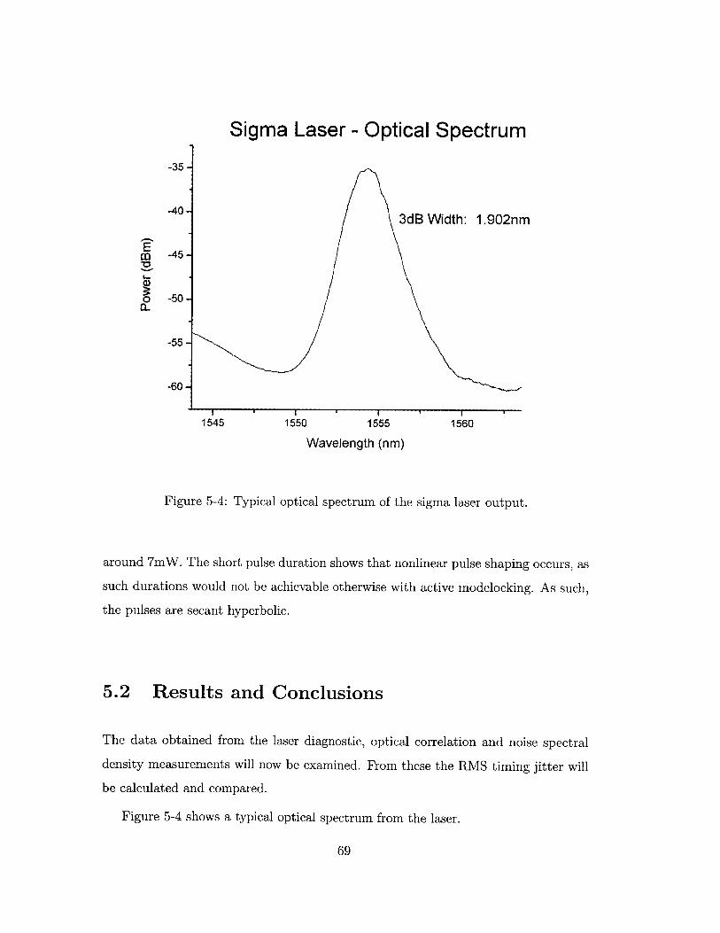
E
(D
0a.
-35 -
-40 -
-45 -
-50 -
-55 -
-60 -
1545
Sigma Laser - Optical Spectrum
3dB Width: 1.902nm
155('
I
1555
Wavelength (nm)
1560
Figure 5-4: Typical optical spectrum of the sigma laser output.
around 7mW. The short pulse duration shows that nonlinear pulse shaping occurs, as
such durations would not be achievable otherwise with active modelocking. As such,
the pulses are secant hyperbolic.
5.2 Results and Conclusions
The data obtained from the laser diagnostic, optical correlation and noise spectral
density measurements will now be examined. From these the RMS timing jitter will
be calculated and compared.
Figure 5-4 shows a typical optical spectrum from the laser.
69

ca
(DC,)
1.0-
0.8-
0.6-
0.4-
0.2 -
--8000
Auto- and Cross-Correlations, 20 nm Filter
-- Auto-- - Cross-
varW(AC) = 1.97 pvarW(XC) = 3.31 p
-4000 0
Delay (fs)4000
S2
s 2
8000
Figure 5-5: Trace of the auto-correlation and cross-correlation of neighboring pulse.
5.2.1 Optical Correlation Measurement Results
The optical auto-correlation and cross-correlations of neighboring pulses are shown in
Figure 5-5. The numerically calculated variance widths, using the data that generated
these traces, are found to be varW(XC) = 3.31ps2 and varW(AC) = 1.97ps2 .
When calculating the timing jitter, it is assumed that neighboring pulses are
uncorrelated. Given that the output pulses originate from different intracavity pulses,
this assumption is expected to be valid.
Using Equation (2.18) and assuming that the pulses are uncorrelated, an RMS
timing jitter calculation results in 819fs. To place conservative bounds on the cal-
culated timing jitter, a p(AT, AT) = +1 correlation assumption results in an RMS
timing jitter of 1158fs, and a p(AT, AT) = -1 correlation assumption results in
70
N_
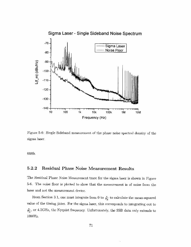
Sigma Laser - Single Sideband Noise Spectrum
-70-Sigma Laser
-80 - Noise Floor
N -90-
-100 -
-110-
-120-
-130-
-140-110 100 1k 10k 100k 1M 10M
Frequency (Hz)
Figure 5-6: Single Sideband measurement of the phase noise spectral density of the
sigma laser.
668fs.
5.2.2 Residual Phase Noise Measurement Results
The Residual Phase Noise Measurement trace for the sigma laser is shown in Figure
5-6. The noise floor is plotted to show that the measurement is of noise from the
laser and not the measurement device.
From Section 3.1, one must integrate from 0 to -- to calculate the mean-squared
value of the timing jitter. For the sigma laser, this corresponds to integrating out to
7, or 4.5GHz, the Nyquist frequency. Unfortunately, the SSB data only extends to
10MHz.
71
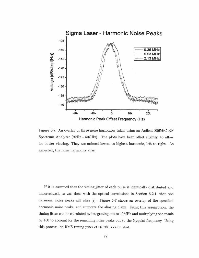
Sigma Laser - Harmonic Noise Peaks*1
-105-
-110-
-115-
-120-
-125 -
-130-
-135 -
-140-I I I'I. -I
-20k
9.35 MHz5.53 MHz2.13 MHz
A~
IN~
-10k 0 10k
Harmonic Peak Offset Frequency (Hz)20k
Figure 5-7: An overlay of three noise harmonics taken using an Agilent 8565EC RF
Spectrum Analyzer (9kHz - 50GHz). The plots have been offset slightly, to allow
for better viewing. They are ordered lowest to highest harmonic, left to right. As
expected, the noise harmonics alias.
If it is assumed that the timing jitter of each pulse is identically distributed and
uncorrelated, as was done with the optical correlations in Section 5.2.1, then the
harmonic noise peaks will alias [9]. Figure 5-7 shows an overlay of the specified
harmonic noise peaks, and supports the aliasing claim. Using this assumption, the
timing jitter can be calculated by integrating out to 10MHz and multiplying the result
by 450 to account for the remaining noise peaks out to the Nyquist frequency. Using
this process, an RMS timing jitter of 2619fs is calculated.
72
Ir
0oMI

5.2.3 Conclusions
The results from each type of measurement are roughly on the same order. A number
of factors are likely to have contributed to the disparity.
The optical correlation measurement is limited in its resolution. For many systems
with low jitter, including the sigma laser using a 10nm bandwidth optical filter (data
not presented), the fractional width change in the cross-correlation is rather small.
This can make it difficult to resolve, and lead to error.
In the residual phase noise measurement, the assumption that the oscillator timing
noise and the laser output noise are uncorrelated may not be accurate. The laser
modelocker is driven by the oscillator, and thus the laser and modelocking oscillator
cannot be totally independent. The assumption that the noise contribution of the
local oscillator is zero is also not exact. It is expected that this source of error,
however, is not very large, considering the specifications of the Poseidon oscillator
(-112 dBc/Hz © 100Hz, -141 dBc/Hz © 1kHz, -161 dBc/Hz C 10kHz, -172 dBc/Hz
L 100kHz). A third source of error is through the coupling of amplitude noise to
phase noise. While the bias was set to suppress amplitude noise, this suppression is
far from perfect, on the order of -15dB [3]. Thus, amplitude noise bleed-through is
expected to contribute to error.
Given the sources of error in this measurement, the experimental results reason-
ably illustrate the relationship between both measurement techniques.
73

74

Chapter 6
Experiments Measuring Timing
Jitter of a Passively Modelocked
Fiber Laser Using Frequency
Discrimination
In this chapter, experiments which use frequency discriminator techniques to measure
timing jitter in a 10MHz fundamentally modelocked P-APM laser are described. The
performance of the frequency discriminator system is observed. The timing jitter of
the system is calculated, based on the measurements made and their limitations.
6.1 Experimental Setup
6.1.1 Passively Modelocked P-APM Fiber Laser System
Figure 6-1 shows the laser system used. Most of the length of the laser consists of
Erbium-Doped Fiber and Dispersion Shifted Fiber (DSF) sections. In these section,
nonlinear polarization rotation via the Kerr Effect occurs1 . This results in higher
'Nonlinear polarization rotation due to the Kerr Effect occurs in the Single-Mode Fiber (SMF)
fiber also. Most of the length of this laser cavity is made up of the Erbium and DSF sections, and
75

Polarizing/2 Isolator V4
__ O+- 00Filter X/2
Polarization Erbium DSFController
90%
10% Output
Figure 6-1: The P-APM 10MHz laser.
intensities emerging from the fiber in one state of polarization, and lower intensities
in a different polarization state. Subsequently, the polarizing isolator is reached, and
different loss is experienced depending on the polarization state, i.e. the intensity.
When the waveplates and polarization paddles are properly biased so that higher
intensities pass through the polarizing isolator with less loss, modelocked operation
is favored [18].
It should be noted that other bias points exist. Very often, near the modelocked
bias points there lies a bias point that causes Q-switching. Additionally, there are
very stable continuous wave (CW) states, where CW modes of operation are favored,
resulting from biasing that suppresses modelocking.
The discrete nature of soliton pulse energies, as shown in Section 4.1 by the Area
Theorem, can also be seen in this system. At sufficient pump energies, on the order
of 80mW and above, the cavity can support multiple pulses per round trip. How the
energy is distributed, i.e. what pulse configurations are over a round-trip period, is
fairly random and extremely hysteretic, as seen by oscilloscope traces. The multiple-
pulse operation is eliminated by reducing the pump power while in a modelocked state
until one pulse per round trip operation (fundamental modelocking) is achieved.
thus we treat nonlinear polarization rotations elsewhere as negligible.
76

The laser was pumped with an SDL MOPA Laser (Model 5762) at 978nm. The
pump beam is coupled into Flexcore fiber and forward pumps the Erbium using a
Gould 980/1550 WDM fiber coupler. The typical pump power level that supported
single-pulse operation was 35mW ± 10mW, depending on the polarization paddle
and waveplate settings. In many cases, the laser would fall out of modelocking as the
pump power was reduced before single-pulse operation could be reached.
Typical average optical output power from the laser in this state was 150iW at
the 10% output port. The pulse parameter width, T, of the output pulses was 520fs
as shown in Figure 6-3.
A typical optical spectrum is shown in Figure 6-2. One may initially assume that
the two lobes on the side are Kelly sidebands [19][20]. However, this may not be
the case. The optical filter being used has a 7.5nm bandwidth, and falls off sharply.
When CW lasing, the spectrum clearly shows where the edges of the filter lie. Those
edges correspond exactly with the dips between the main peak and side peaks of the
modelocked spectrum. Thus it seems that the filter causes this feature.
Given the Fourier transform of a square function, one expects this square filter
shape to cause lobes to appear in the time domain, on either side of the pulse. (The
Fourier transform of a square is a function of the form si"C.)) The auto-correlationX
of the pulse is shown in Figure 6-3, and indeed, the lobes do appear.
Traces for various ranges over the RF spectrum are given in Figure 6-5. The even
distribution of the energy into the harmonics shown in the 0Hz to 2GHz trace gives
indication that there is one pulse, not multiple pulses, per round-trip time. The roll off
of this plot is due to the bandwidth of the RF amplifiers (0-1GHz) used in detection.
The trace from 0Hz to 200MHz shows the uniformity of the harmonic peaks. The
final trace is a close-up of the fundamental repetition rate peak, and shows that this
frequency is 10.378MHz.
6.1.2 Frequency Discriminator Setup
A frequency discriminator measurement system, shown in Figure 6-6 was constructed
to measure the timing jitter. The P-APM laser output was split using a 20%-80%
77
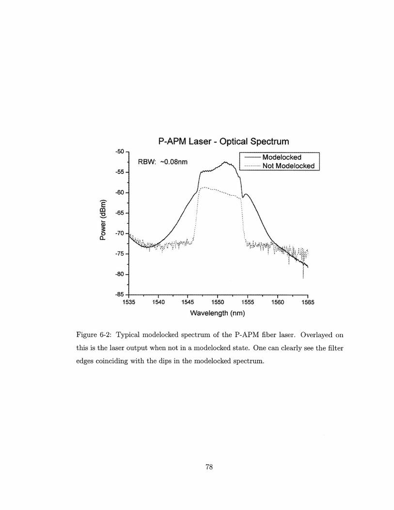
P-APM Laser - Optical Spectrum-50-
RBW: ~-O.08nm Modelocked-55- ------ Not Modelocked
-60--5-
0 -7
-75 -
-80-
1535 1540 1545 1550 1555 1560 1565
Wavelength (nm)
Figure 6-2: Typical modelocked spectrum of the P-APM fiber laser. Overlayed on
this is the laser output when not in a modelocked state. One can clearly see the filter
edges coinciding with the dips in the modelocked spectrum.
78

0.007-
0.006-
0.005-
0.004 -
0.003-
0.002
0.001
0.000
-6000 4
P-APM Laser - Auto-Correlation Trace
- Auto-Correlation Trace- - Sech Fit
Pulse Width (Fit): 520 fs
000 -2000 0 2000 4000 6000
Time (fs)
Figure 6-3: Typical auto-correlation of the P-APM fiber laser. A dashed line shows
a secant hyperbolic fit to the auto-correlation trace. The bumps in the wings of the
pulse are attributed to the optical filter shape.
P-APM Laser - Oscilloscope Trace of Pulse P-APM Lasr - Osciloo Tra of PuP-APM Las --...--- scoE-Ta- fP
a
OA .
0 3.
0.2.
0.1.
0.0-
0It
-40:On -20 On 0.0
Time (s)20On
04,
.200n *100n
0.13.
0.2-
0.1.
00.
40.On 00Time (s)
kse Trnin
100.On 200.0n
Figure 6-4: Digital Oscilloscope trace of a single optical pulse, and the optical pulse
train.
79
C,)

P-APM Laser - RF Spectrum
RBW. 30Hz
10.374 10.376 10.378
Fundamental Peak*10.378 MHz
'0
0.
10,380 10.382
-40-
460.
40-
120 50 50
Frequency (MHz)
P-APM Laser - RF SpectrumRBW: 100kHz
.1. 1 I.100 150 200
Frequency (MHz)
P-APM Laser - RF Spectrum
RBW: 100kHz
-120 ' jr T11' w Fl i ' Eorr , 1 revWq
0.0 0.5 1.0 1.5 2,0
Frequency (GHz)
Figure 6-5: Various plots of the RF spectrum of the laser output.
80
-40 -
-40-
-80-
-100 -
-120-
CO
4A
40
I.80
-100
rA )1H

coupler. The 20% path was split again with a 1%/99% coupler, where the 1% port
went to the optical spectrum analyzer and the 99% port went to the optical correlator.
The 80% port served as the input to the frequency discriminator setup. This port was
split with a 50%/50% coupler. One output was fed to the LO detector. The other
port is delayed by a changeable fiber delay line, and then fed to the RF detector.
Both the RF and LO detector are Discovery Semiconductor DSC40S detectors with
a 16GHz bandwidth, chosen to match each other as closely as was possible in their
responsivity. The delay lines were made of Corning LEAF fiber, with a dispersion of
5 ps/nm/km.
The detected signals were then filtered by a Mini-Circuits bandpass filter (Model
SBP-10.7, 10MHz CWL, 3.7MHz BW), and then by a low-pass filter (Mini-Circuits,
Model SLP-750, 750MHz). The resulting signal was then amplified by two cascaded
low noise amplifiers (Mini-Circuits, ZFL-1000LN, +20dB gain, NF 2), attenuated
to appropriate levels to avoid amplifier compression, amplified by another amplifier
(Mini-Circuits, Model ZKL-2, +29dB gain, NF 5), DC blocked (Arra, 1-9572E), phase
delayed in the RF arm (two Arra delays, Model 3448B, 27r 0 1GHz range each), and
fed into the mixer (Mini-Circuits, Model ZFM-4, Level +7dBm) ports. Immediately
before the mixer port, a -20dB tap (Mini-Circuits, Model ZFDC-20-5) was placed to
monitor the power into the mixer to ensure optimal mixing. The mixer output was
filtered with another low-pass filter (Mini-Circuits, Model SBP-3, 3MHz) leave a DC
signal.
6.1.3 Determining K0
By measuring the spectral noise density of the voltage, one can calculate the timing
jitter spectral density. This calculation requires the conversion from voltage noise
spectral density to phase noise spectral density, and thus a measurement of the con-
version constant, K0, is needed, as shown in Equation (3.28).
This is done by adjusting the RF path length until an average of zero voltage at the
output is seen. This average was viewed using an averaging function on a Tektronix
digital oscilloscope (Model: TDS 380, 400MHz BW). Once this zero average voltage
81

Band-Pass DCFher Delay AE, AT Filter Amplifiers -4dB Blc k 20dB Tap
LO Photo- -10<11 AmplifierDetector Low-pass IF SignalLaser 3dBilter Mixer
Coupler Photo- Low-Pass Amplifier Low-PassRF Detector Filter -20dB Phase Delays Filter
AE, AT Band-Pass Amplifiers o-9dB C 20dB lap
Filter Atten. Block
Figure 6-6: The frequency discriminator system used for these measurements.
is found, the RF path length was adjusted small amounts using the phase delay, and
the delay amount (in radians) and voltage recorded. The slope of a linear fit to these
data points provided the slope of the voltage vs. phase, which is precisely K0.
This process was performed out before each spectrum is taken. Each set of cali-
bration data consisted of at least four data points.
6.2 Results and Conclusions
Using the frequency discriminator, voltage noise spectral densities were taken for de-
lay lengths of Om (noise floor), 500m, 1000m, 2000m, 4000m, 5000m, and 6000m. The
complete set of data is shown in Section C.1 in terms of the voltage noise spectral
density. Figure 6-7 presents two single sideband spectra, assuming no pulse corre-
lation. Because the pulse correlation is not known, single sideband measurements,
C(fm), can not be plotted with quantitative accuracy, but can provide qualitative
information.
6.2.1 Sensitivity
One will immediately notice the oscillations that begin to appear at higher frequencies.
In Section 3.3.2, the sensitivity for a frequency discriminator system was derived,
concluding that the sensitivity has a siIx) dependence. The oscillations that appear
82

Single Sideband Plot Assuming Zero Correlation-80,
10 100
-1000m DelayNoise Floor
1k 10k
.. . . . . . .. . . .
100k 1M
Frequency (Hz)Single Sideband Plot Assuming Zero Correlation
-80I
5000m Delay-- Noise Floor
I10 100 1k 10k 100k
Frequency (Hz)
Figure 6-7: Frequency discriminator single sideband plot of timing jitter, assuming
no correlation. Delay length is 1000m / 5.Ops (top), and 5000m / 25.Ois (bottom).
83
-g0-
N
-100-
-110-
-90-
NIcoV
S-J
-100-
-110-
IM
I

in the data match up extremely well with the theoretically predicted sensitivity.
6.2.2 Extracting the Correlation as a Function of Delay
Equation (3.28) shows the correlation function in the expression for the voltage fluc-
tuations. It has been shown in [9] that for a fundamentally modelocked laser, the
mean-squared jitter, i.e. the correlation function, should be:
D D(AT(O)A T(nTR)) = (1 - D)_e-2TR I (6.1)
2'1TR 2SYTR
where the approximation holds when -yTR << 1.
Because this exponential decay of the correlation affects the noise spectral den-
sity, an attempt can be made to extract this correlation from the data. One may
integrate the timing noise spectral densities for each delay length, and observe the
resulting dependence of the timing jitter on delay length. Ideally, this will result in
a measurement of -yTR. Considering the si"Cx) sensitivity limitations of the frequencyX
discriminator measurement, a portion of the spectrum must be chosen where, for ev-
ery delay length, the system is sensitive enough to take valid data. Figure 6-8 shows
the sensitivity plots for the time delays used in this experiment. From this, it is
concluded that the frequency range from 175kHz to 191.7kHz is most appropriate.
The resulting calculated RMS timing jitter values over this bandwidth are plotted
in Figure 6-9 as a function of delay length. As expected, the integrated timing noise
increases as the correlation decreases. However, the expected 1 - e Rt dependence is
not seen.
The extraction of the correlation coefficient would benefit from careful choice of
delay lengths to maximize the overlap range. High-resolution plots of the overlapping
frequency band to be integrated would also greatly improve the accuracy.
6.2.3 Timing Jitter Results
Although the noise spectral density results do not allow the extraction of a number for
the timing jitter, attempts were made to extract limits for the timing jitter, making
84

6000m-5000m
0 4000m2000m1000m
..20 500m
-40
4 0
-so-
-100.50.0k 100,0k 150.0k 200.0k 250.0k 300.0k 350.0k 400.0k
Frequency
Figure 6-8: Plot of the sensitivity of the frequency discriminator as a function of
frequency for various delay lengths. The first null frequency decreases as the delay
length is increased.
85

Integrated Timing Jitter over 175kHz-1 92kHzas a Function of Delay
U
0
a
a0
I I I * I * I * I I
0 1000 2000 3000 4000 5000Delay Length (m)
6000 7000
Figure 6-9: Plot of the integration over 175kHz to 191.7kHz of
data, as a function of delay length.
SAT,AT - SAT(O),AT(td)
86
Co
4)
C)
2*1=
-
4)
8.OOE-020 -
T00E-020 -
6.OOE-020 -
5.0OE-020 -
4.00E-020 -
3.00E-020 -
2.OOE-020 -
1.00E-020 -
0.00E+000 -
-1.00E-020
a

certain assumptions.
The first calculation made was to plot the timing noise spectral density noise
floor, and integrate out to the Nyquist frequency. This result will give some idea of
the minimum amount of RMS timing jitter one can measure. Of course, the actual
minimum is dependent on the spectral distribution of the timing jitter. Either way,
an integral of the noise floor, using Equation (3.5), results in a timing jitter of 168ps.
A similar calculation for the 6000m delay length, executed without " correction
or regard to the noise floor, yields an RMS timing jitter of 248ps.
Given the lack in the data of any spectral characteristics predicted by the theory,
as well as many other uncertainties, it is not believed that these numbers are valid.
6.2.4 Conclusions
This set of experiments produced inconclusive results.
It seems that the data is masked by the noise floor at low, rising out at higher
frequencies. This seems strange, considering that the frequency discriminator should
show maximal sensitivity at low frequencies, and that a passively modelocked laser
should exhibit a timing noise spectral density that is greatest at lower frequencies.
Also, it appears that the noise spectrum first "rises out" of the noise floor at in-
creasingly higher frequencies as the delay is lengthened. One would expect that longer
delays would increase the sensitivity a lower frequencies and cause the "rising out"
frequency to decrease as the delay is lengthened. This leads to the conclusion that
data that appears to be above the noise floor, while clearly related to the sensitivity
of the frequency discriminator, is not timing jitter in the optical pulse train.
More specifically, it is believed that the spectral densities are dominated by extra-
neous noise. This conclusion is based on several observations. In attempts leading up
to acquiring the data presented, the filters in the frequency discriminator arms were
place after the amplifiers. In those preliminary data sets, the sensitivity oscillations
in the noise spectral density were not as clearly seen.
The filters were moved before the amplifiers in order to increase the average power
at the mixing to necessary levels for the mixer to operate correctly. However, by
87

moving the filters before the amplifiers, all of the unwanted noise from the amplifiers
is now allowed to reach the mixer, and thus the mixing products of the amplifier noise
shows up in the data. Additionally, large integrated spectral density numbers were
seen. Therefore, it is believed that the timing jitter is below the noise floor. Filtering
earlier in the frequency discriminator should improve performance.
The noise floor also seems to show oscillatory behavior in the MHz range. This
behavior seems to appear around 2-3MHz, and is attributed to the 3 MHz bandwidth
of the 3MHz band-pass filter after the mixer and the 3MHz bandwidth of the 10.7MHz
bandpass filters. Obviously, the filters interfere with results at these frequencies.
Ideally, filters should be used that flatly pass out to the Nyquist frequency.
If indeed it is laser timing noise that is rising out of the noise floor, the shape of
the optical filter may be partly responsible for the disparity between the experimental
and theoretical characteristics of the noise spectral density. The filter drops off very
quickly, so the expansion of the filter shape to second order in the timing noise spectral
density derivation in Section 4.2 may neglect significant higher-order contributions.
In Section 5.1.3 it was observed that the filter greatly effecting the timing jitter, so
it seems plausible that the filter may play a significant role here.
At this point, the only fundamental limitation of the frequency discriminator
seems to be the bandwidth limitations.
6.2.5 Future Work
Several future experiments can be pursued as extensions of this work.
The simplest is to further optimize the current setup. The laser system would
benefit greatly from a more appropriate optical filter. Much room for optimization
of the frequency discriminator to decrease the noise floor also exists. Although this
thesis showed that, theoretically, using laser output harmonics will not improve the
system's sensitivity 3.3.2, this should be verified experimentally.
Another question arose during this work: One detects the optical pulse train, and
looks at the phase noise as an indication of the optical pulse train noise. When one
observes a higher harmonic of the pulse train, how does one interpret the phase noise
88
at a position in time corresponding to a position between pulses in the optical pulse
train? Future work may pursue this and similar questions.
Ultimately, the interesting application of the frequency discriminator is to measure
the timing jitter of quiet passively modelocked laser systems. The current P-APM
laser, modified for regenerative phase modulation [21] qualifies as one of these systems,
and measurements of this laser's noise will be pursued.
89

90

Chapter 7
Summary
In this work, optical correlation, residual phase noise, and frequency discriminator
techniques for measuring the timing jitter of an optical pulse train were reviewed.
Experiments comparing the results of an optical correlation and residual phase noise
measurement were compared, and reasonably close results were found.
Soliton perturbation theory was also reviewed, and observed for the case of active
and passive modelocking. Experiments using the frequency discriminator technique to
measure the timing jitter of a polarization additive-pulse modelocked fiber laser were
carried out. The current experimental results allowed for few concrete conclusions;
however, there are many avenues left to explore to improve the performance of the
system and the results of experiments.
91

92

Appendix A
Physical Derivations Reference
A.1 Dispersion
The combined effect of material and waveguide dispersion are important in consider-
ing fiber laser operation, and are vital to the existence of solitons. The relationship
between two parameters used to express the group velocity dispersion (GVD) of a
particular dielectric waveguide is sought here. This section is based on [14].
For a wave with frequency w travelling down a waveguide there is an associate
wavevector, 3(w). We expand # in a Taylor Series about zero frequency in order to
express the wavevector's dependence on frequency as a sum of polynomials:
O(W) = O(W = 0) + W + - W2 +...9 .W=0 .a2. W=0
113(w) = /o + /'w + -"w 2 + ... (A.1)
2
)3" is the GVD, which describes the curvature of the wavevector's dependence on
frequency, and is most commonly given in units of ps 2/km.
The D parameter is another expression of the GVD, and is related to #" in the
following way:
2ircD = 27r" (A.2)
93

D is normally given in units of ps/nm/km. Normal dispersion, where longer
(red) wavelengths propagate faster than shorter (blue) wavelengths, corresponds to
/ > 0, D < 0. Anomalous dispersion, where short (blue) wavelength propagate faster
than longer (red) wavelengths, corresponds to / < 0, D > 0.
94

Appendix B
Mathematical Review
B.1 Review of Basic Probabilistic Quantities and
Concepts
This section is primarily intended as a reference to the reader. Most of the information
for this section is taken from [22]. We follow this source's notation, where we write
random variables with capitalized variables, and nominal values of that variable with
lowercase variables.
B.1.1 Probability Density Function
The Probability Density Function (PDF) describes how likely a particular random
variable is to take on a value that falls within a given range. Thus, if we consider
random variable X, which has a PDF called fx(x), then the probability that X will
take on a value between x and x + 6 is given by:
P(x < X < x +J) = j dxfx(x) (B.1)
For two random variables, X and Y, we can define the joint PDF, describing how
X and Y vary with respect to each other. We write this as fxy(x, y). From this,
we can find the PDFs of each variable alone, the marginal PDFs. For example, the
marginal PDF of X is found as follows:
95

fx(x) = fxy(x, y)dy (B.2)
B.1.2 Expectation
The expectation, or first moment, of a random variable describes the mean, or average
value that a random variable will take on. The expectation of random variable, X,
is written as E[X] or as (X).
One can also take expectations of functions of random variables. For a function
of continuous random variable, X, the expectation is given as:
E[g(X)] = (g(X)) = J g(x)fx(x)dx (B.3)
For functions of continuous random variables, X and Y, the expectation is given
as:
E[g(X, Y)] = (g(X, Y)) = J J g(x, y)fxy (x, y)dxdy (B.4)
B.1.3 Variance and Mean-Squared Value
The variance of a random variable describes how spread out the probability distribu-
tion is - how it "varies". The variance of random variable, X, is written as varX and
is defined as:
var(X) = E[(X - E[X])2 ] = E[X2 ] - (E[X])2 = (X 2 ) - (X)2 (B.5)
which we see is a function of the first and second moment. Notice that, when the
expectation is zero, the variance equals the mean-squared value, (X 2).
One can take variances of functions of random variables, in an analogous way to
that shown in Equation (B.3) and Equation (B.4).
96
B.1.4 Moments
Generally, one can talk about the moments of a PDF, where the nth moment is given
as E[X"]. Knowledge of the value of every moment of a given PDF will uniquely
specify the PDF.
B.1.5 Covariance and Correlation Function
As the variance describes how a random variable varies, the covariance describes how
two random variables vary relative to each other. The covariance of random variables,
X and Y, is given by:
cov(X, Y) = E[(X - E[X])(Y - E[Y])] = E[XY] - E[X]E[Y] = (XY) - (X)(Y)
(B.6)
Notice that when either the expectation of X or Y are zero, the covariance is equal
to the correlation function for X and Y, (XY).
B.1.6 Correlation Coefficient
The correlation coefficient, p(X, Y), is a normalized version of the covariance. jp(X, Y) Iexpresses the degree of correlation and ranges from 0 to 1, and the sign of p(X, Y)
expresses the sign of the correlation (whether X and Y tend to have the same or
opposite signs). The correlation coefficient is given as:
(X'Y) cov(X, Y)
var(X)var(Y)
Note that perfect correlation does not imply that the random variables have the
same PDFs. Also note that the correlation coefficient and the correlation function
are related, but are not the same thing.
B.1.7 Variance of the Sum of Two Random Variables
For the general random variables, X and Y, the variance of their sum is given as:
97

var(X + Y) = var(X) + var(Y) + 2cov(X,Y) (
or in terms of mean-squared values and correlation functions, we see the expectation
cancel and find:
((X + Y) 2 ) = (X 2) + (Y 2) + 2(XY) (B.9)
B.1.8 Independent Random Variables
Two random variables, X and Y, are said to be independent when the probability
distribution of one is not effected by knowledge of the other variable. Independence
is formally defined when the joint PDF of X and Y are related to the marginal PDFs
of X and Y by the following:
fx~y (x + y) = fx(x)fy (y) (B.10)
B.1.9 A Few Consequences of Independence
Independence leads to the following consequences:
1. The cov(X, Y) = 0. X and Y are uncorrelated.
2. The PDF of the sum of X and Y, call it Z, is the convolution of the PDF of X
and the PDF of Y:
(B.11)fz(z) J fx(x)fy (z - x) = J dyfy(y)dxfx(z - y)
3. The variance of Z equals the sum of the variances of X and Y:
var(X + Y) = var(X) + var(Y)
98
(B.8)
(B. 12)

and thus:
((X + Y) 2 ) = (X 2) + (Y 2 ) (B.13)
B.1.10 Central Limit Theorem
The central limit theorem, an expression of the strong law of large numbers, states
that the sum of a large number of independent random variables tends to have a
distribution that is Gaussian, regardless of the probability distribution of each inde-
pendent random variable.
B.2 Pulse Width Measures
In this section, we summarize the analytic and numerical relationship between various
measures of pulse width.
B.2.1 Definition of Widths
One can indicate the width of a pulse in different ways. Here we classify some of
those ways as the pulse width, the full-width half-maximum, and the variance width.
Pulse Width
The definition of pulse width varies from pulse shape to pulse shape. The pulse width
is consistently labelled as T or ri.
Full-Width Half-Maximum
The full-width half-maximum takes the usual definition, which is the width of the
pulse at one half of its maximum height. For pulse Ii(t), We notate the full-width
half-maximum as FWHM(I).
99

Variance Width
The variance width is defined using an analogy with probability calculations. We
normalize the pulse shape, and treat it as though it were a PDF for a random variable.
We then calculate the variance of that PDF.
Notationally, for pulse Ii(t), we denote the variance width as varW(Ij), where we
suppress the unnecessary argument of the function.
Notice that in our notation, the argument of varW() can be written normalized,
but we do not require it. In calculating varWO, however, we must be sure to take
the variance of the normalized argument of the function. Failing to do so will lead to
factors, specifically, inverse normalization constants, that we do not want.
B.2.2 Gaussian Widths
For gaussian pulses, we consider the form:
t2
f (t) = . 2- (B.14)
where T we call the pulse width.
We find that the FWHM scales linearly with the pulse width, as expected, and
that the variance scales with the square of the pulse width. We can solve these
relationship analytically, and we find:
FWHM(f) = 2lrn(2) (v'2r) (B.15)
varW(f) = 2T 2 (B.16)
B.2.3 Secant Hyperbolic Widths
For secant hyperbolic pulses, we consider the form:
f(t) = sech ) (B.17)
100
where r we call the pulse width.
We find that the FWHM also scales linearly with the pulse width, and that the
variance scales with the square of the pulse width. The coefficients resulting from
numerical calculations are included in the following equations:
FWHM(f) = 2 .80 00T (B.18)
varW(f) = 2.461T 2 (B.19)
101

102

Appendix C
Data
C.1 Frequency Discriminator Data
In this section, the raw data as taken for the experiments in Chapter 6 is presented.
Each plot contains the single sideband voltage noise spectral density for a specific
delay, along with the noise floor and theoretical sensitivity curve.
103

Data for 500m Delay-80 -
-go-90 -
-100-
-110-
-120-
500mFNoise Floor0
C)
0
10
-90 -
-100-
-110-
-120- A
'ILi~~J~iIIi1JRIII I
~"~r r
100
ml
1'
ik 10k 100k iM
Frequency (Hz)Data for 1 000m Delay
ise Floor
I10 100
W'~P1 1
Ik 10k 100k
Frequency (Hz)
Figure C-1: Voltage noise spectral density and sensitivity plots for 500m (2.5pts) and
1000m (5.0ps) delay.
104
V~t~X~4li.
0
-20
-40
-60
-80
-100
-120
-140
-160
-180
-200
0
-20
-40
-60
-80
-100
-120
-140
-180
-180
-200
(I)
0)2~
IM
- I
. ?T-
I All,
.. . . .. .
-
-)
c£2
I
-80 -1
-10- No

Data for 2000m Delay
2000mNoise Floor
-80-
-90-
-100 -
0
110
-110-
0
10 100
Iik 10k
0
-20
-40
-60
-80
-100 %
-120 E
-140
-160
-180
-200100k IM
Frequency (Hz)Data for 4000m Delay
iF4000moNoise Floor
fi
] I
100 1k 10k 100k IM
Frequency (Hz)
Figure C-2: Voltage noise spectral density and sensitivity plots for 2000m (10.0p-s)
and 4000m (20.Ops) delay.
105
I
-8 0 -i
-o
0
-20
-40-90-
-100-
-110-
-120 -
-60
-80
-100
-120
-140
4'
0)
C
0
1~-f~.
10
-160
-180
-200
- --------
tit

Data for 5000m Delay
-5000mNoise Floor
-80-
-90
0-100
-110-C14)012
(N
~I
AA!................ 1........ I
10 100 1k 10k
M
~1
100k 1MFrequency (Hz)
Data for 6000m Delay
6000M-- Noise Floor
j
10 100 1k
'A
IM10k 100kFrequency (Hz)
Figure C-3: Voltage noise spectral density and sensitivity plots for 5000m (25.0ps)
and 6000m (30.Ops) delay.
106
iti
0
-20
-40
-80
-80wE
-100 Z!-120
4)-140 CO)
-160
-180
-200
-80 -N
-90-
0 -100-
CO
CO
-110
-120 -
0
-20
-40
-60
-80
-100 >
-120 ca)
.1-140
-160
-180
-200
I
'.I

Bibliography
[1] Paul W. Juodawlkis, Jonathon C. Twichell, Gary E. Betts, Jeffrey J. Hargreaves,
Richard D. Younger, Jeffrey L. Wasserman, Fredrick J. O'Donnell, Kevin G.
Ray, and Richard C. Williamson. Optically sampled analog-to-digital converters.
IEEE Transactions On Microwave Theory and Techniques, 49(10):1840-1853,
October 2001.
[2] Robert H. Walden. Analog-to-digital converter survey and analysis. IEEE Jour-
nal on Selected Areas in Communcations, 17(4):539-550, April 1999.
[3] Matthew Edward Grein. Noise and Stability of Actively Modelocked Fiber Lasers.
PhD dissertation, Massachusetts Institute of Technology, Department of Electri-
cal Engineering and Computer Science, 2002.
[4] Leaf Alden Jiang. Ultralow-Noise Modelocked Lasers. PhD dissertation, Mas-
sachusetts Institute of Technology, Department of Electrical Engineering and
Computer Science, May 2002.
[5] Darpa/eto photonic a/d converter technology (pact) kick-off meeting. MIT-
Lincoln Laboratory, Lexington, MA, 1999.
[6] Erich P. Ippen. Principles of passive mode locking. Applied Physics B: Lasers
and Optics, 58:159-170, 1994.
[7] Leaf Alden Jiang. A comparison of various technologies for optical autocor-
relations of picosecond pulses at 1.5pm. Paper written in fulfillment of Area
Examination at M.I.T., 2001.
107
[8] Robert W. Boyd. Nonlinear Optics. Academic Press, San Diego, California, first
edition, 1992.
[9] Farhan Rana, Harry L. T. Lee, Rajeev J. Ram, Matthew E. Grein, Leaf A.
Jiang, Erich P. Ippen, and Hermann A. Haus. Characterization of the noise and
correlations in harmonically mode-locked lasers. Journal of the Optical Society
of America, 19(11):2609-2621, November 2002.
[10] Paul W. Juodawlkis, Jonathon C. Twichell, Jeffrey L. Wasserman, Gary E. Betts,
and Richard C. Williamson. Measurement of mode-locked laser timing jitter by
use of phase-encoded optical sampling. Optics Letters, 26:289-291, 2001.
[11] D. von der Linde. Characterization of the noise in continuously operating mode-
locked lasers. Applied Physics B, 39:201-217, November 1986.
[12] Ryan P. Scott, Carsten Langrock, and Brian H. Kolner. High-dynamic-range
laser amplitude and phase noise measurement techniques. IEEE Journal On
Selected Topics In Quantum Electronics, 7(4):641-655, July 2001.
[13] Hewlett-Packard. Product note 11729c-2: Phase noise characterization of mi-
crowave oscillators. Technical report, Hewlett-Packard, 1985.
[14] Kohichi Robert Tamura. Additive Pulse Mode-Locked Erbium-Doped Fiber
Lasers. PhD dissertation, Massachusetts Institute of Technology, Department
of Electrical Engineering and Computer Science, 1994.
[15] A. Hasagawa and F. Tappert. Transmission of stationary nonlinear optical pulses
in dispersive dielectric fibers. Applied Physics Letters, 23:142-144, 1973.
[16] Hermann A. Haus and Antonio Mecozzi. Noise of mode-locked lasers. IEEE
Journal of Quantum Electronics, 29:983-996, 1993.
[17] M. E. Grein, L. A. Jiang, H. A. Haus, E. P. Ippen, C. McNeilage, J. H. Searls,
and R. S. Windeler. Observation of quantum-limited timing jitter in an active,
harmonically mode-locked fiber laser. Optics Letters, 27:957-959, 2002.
108

[18] M. Hofer, M. E. Fermann, F. Haberl, M. H. Ober, and A. J. Schmidt. Mode
lcoking with cross-phase and self-phase modulation. Optics Letters, 16:502-504,
1991.
[19] S.M.J. Kelly. Characteristic sideband instability of periodically amplified average
soliton. Electronics Letters, 28:806-807, 1992.
[20] Michael L. Dennis and Irl N. Duling III. Experimental study of sideband genera-
tion in femtosecond fiber lasers. IEEE Journal of Quantum Electronics, 30:1469-
1477, 1994.
[21] M. Margalit, C. X. Yu, S. Namiki, E. P. Ippen, and H. A. Haus. Harmonic
mode-locking using regenerative phase modulation. IEEE Photonic Technology
Letters, 10:337-339, 1998.
[22] Dimitri P. Bertsekas and John N. Tsitsiklis. Introduction to Probability. Pre-first
edition, 2002.
109