timed coloured petri nets for performance evaluation of
TRANSCRIPT

HAL Id: hal-01054268https://hal.inria.fr/hal-01054268
Submitted on 5 Aug 2014
HAL is a multi-disciplinary open accessarchive for the deposit and dissemination of sci-entific research documents, whether they are pub-lished or not. The documents may come fromteaching and research institutions in France orabroad, or from public or private research centers.
L’archive ouverte pluridisciplinaire HAL, estdestinée au dépôt et à la diffusion de documentsscientifiques de niveau recherche, publiés ou non,émanant des établissements d’enseignement et derecherche français ou étrangers, des laboratoirespublics ou privés.
Distributed under a Creative Commons Attribution| 4.0 International License
Timed Coloured Petri Nets for Performance Evaluationof DSP Applications: The 3GPP LTE Case Study
Laura Frigerio, Kellie Marks, Argy Krikelis
To cite this version:Laura Frigerio, Kellie Marks, Argy Krikelis. Timed Coloured Petri Nets for Performance Evaluation ofDSP Applications: The 3GPP LTE Case Study. 19th IFIP WG 10.5/IEEE International Conference onVery Large Scale Integration (VLSI-SoC), Oct 2008, Rhodes Island, India. pp.114-132, �10.1007/978-3-642-12267-5_7�. �hal-01054268�

Timed Coloured Petri Nets for Performance Evaluation
of DSP Applications: the 3GPP LTE Case Study
Laura Frigerio1, Kellie Marks
2, Argy Krikelis
2
1Dipartimento di Elettronica e Informazione
Politecnico di Milano
Milano, Italy
2European Technology Center
Altera Corporation
High Wycombe, United Kingdom
{kmarks,akrikeli}@altera.com
Abstract. In this paper we propose the use of Timed Coloured Petri Nets for
the Performance Evaluation of Hardware/Software systems for DSP
applications. Complex systems on chip, composed by hardware and software
parts, are often required to meet strict timing constraints, both in terms of
throughput and latency. However, the verification of the suitability of a system
configuration can usually be performed only after the integration of the
hardware and software components, when design modifications and
optimizations are particularly expensive. This article proposes a framework to
evaluate the performance of HW/SW systems in which Timed Coloured Petri
Nets can be exploited in the early phases of the design. The framework is tested
by modelling the Physical Uplink Shared Channel (PUSCH) bit-rate receiver
portion of 3GPP (3rd Generation Partnership Project) LTE (Long Term
Evolution) standard, the next generation of 3G wireless systems.
Introduction
Complex DSP systems nowadays include heterogeneous hardware and software
components, like multithreaded CPUs, hardware accelerators and fast
interconnections. Due to the systems complexity and to the time-to-market pressure,
IP (Intellectual Property) based methodologies are often used to reduce the
development time and enhance module reuse [1].
Embedded systems for DSP applications have strict constraints on performance that
designers try to meet by efficiently combine pre-verified IPs and ad-hoc
implementations. However, the evaluation of the system performance, in order to
verify the system throughput and latency, is usually very difficult due to both the high
degree of concurrency and the heterogeneity of modules. The system verification can

2
therefore be completed only in final stages of the development, when the hardware
and software modules are integrated into the system. At this stage however, very little
flexibility is left for optimizations and problems in meeting the required constraints
lead to expensive and time consuming modifications of the systems.
For this reason this paper presents a framework for the early evaluation of the system
performance, that can be used to tune and improve the system design before the actual
integration of the components takes place.
Different methods can be used to evaluate the performance of a system and can
generally be classified in 1) simulation techniques and 2) formal models. Simulation
techniques provide information on the system behaviour by tracing the results
obtained when applying stimuli to a system model. Pure simulative approaches using
for example the SystemC Library have been applied in [2] and [3]. However,
simulation approaches alone, cannot provide information on system properties like the
absence of deadlocks or system bottlenecks.
Formal models describe the system in a mathematical form and can provide accurate
information on its behaviour. Example of formal models used for performance
evaluation are Markov processes [4], Queuing Networks [5] and Timed Petri Nets [6].
In this paper, we consider Timed Petri Nets since they are especially suited for
describing HW/SW systems in general and DSP applications in particular. First of all,
Petri Nets are an intuitive and powerful way to define concurrent and asynchronous
processing, useful to describe HW/SW systems. Moreover, with respect to other
methods that consider Stochastic timing models only, Petri Nets allow to consider
both Deterministic and Stochastic timing models. In DSP applications, where IP
blocks are often used in the design, the availability of Deterministic times allows to
build accurate models, since the exact timing required to process input data is often
available (e.g. number of clock cycles of an hardware module) and can be considered
in the model. Finally, several tools are provided to support both the extraction of
analytical properties and the simulation of Petri Nets models.
Petri Nets have been used to model a broad range of applications (refer to [7] for
examples of industrial use). They have also been used to model digital hardware
(many references can be found in [8]). In the context of SoC, the description of
communication infrastructure [9] and the formal verification of the implementation
[10] have been considered. In this paper, Timed Coloured Petri Nets (TCPN) are used
to evaluate the Performance of Hardware/Software systems in early phases of the
system design. The use of Coloured Petri Nets enriches the timing description with
high level elements, such as complex data types and hierarchy decomposition.
Differently from other works on HW/SW systems based on Petri Nets (like [11], [12],
[13]), Petri Nets are not used to support the system design or partitioning, but to
perform a rapid Performance Evaluation at IP-blocks granularity, by seamlessly
integrate HW and SW models.
The rest of the paper is organized as follows. The next Section provides the formal
definition of the Timed Coloured Petri Nets (TCPN) used thorough the paper. A
framework to model a HW/SW system with Petri Nets is then introduced. The
following Section describes the 3GPP LTE application, used as a case study to verify
the proposed framework. The reference HW/SW platform is then presented followed
by the description of the mapping of the LTE application on it, using the Petri Net
framework previously introduced. The following Section compares the results

Timed Coloured Petri Nets for Performance Evaluation of DSP Applications: the 3GPP LTE
Case Study 3
obtained by applying the Petri Net model to those obtained by the integration of the
hardware and software systems. Finally, last Section concludes the work.
Formal definitions
Coloured Petri Nets are an extension of classical Petri Nets, introduced by C. A. Petri
[14]. A Coloured Petri Net is defined [15] as a nine-tuple ( )SEGCNATPCPN ,,,,,,,,Σ= , where:
1. Σ is a set of non-empty types, also called colour sets.
2. P is a finite non-empty set of places.
3. T is a finite non-empty set of transitions
4. A is a finite non-empty set of arcs such that: Ø=∩=∩=∩ ATAPTP
5. N is a node function, defined from A into PTTP ×∪× , which maps each arc into
a tuple where the first element is the source node and the second element is the
destination node.
6. C is a colour function, defined from P into Σ, which means that C maps the place p
to a colour set;
7. G is a boolean expressions, called guard function, which maps the transition t to
the Boolean function needed to be evaluated as “true” to enable the transition;
8. E is an arc expression function. A transition is enabled if there exists, for each
input arc, a token in the input place bounded to that arc.
9. S is the initialization function, which specifies the initial state of the Petri Net.
The initial marking M0 assigns to the place the initial (coloured) Tokens. For a formal
definition, refer to [15]. In Timed Coloured Petri Nets, transition occurrences fire in
’real-time’ associated with each occurrence of each transition. In this paper we
consider deterministic (D-times) nets, where the times are deterministic [6]. Any
enabled transition starts its firing in the same instant in which it becomes enabled.
Each firing can be considered as a three phase event; first, the (coloured) tokens are
removed from the input places as indicated by the arc functions of the firing
occurrence, the second phase is the firing time period, and when it is finished,
(coloured) tokens are deposited to output places as indicated by the arc functions of
the firing occurrence. If a transition occurrence becomes enabled while it is firing a
new independent firing cycle begins.
Formally, a Timed Coloured Petri Nets is a couple TCPN = (CPN, f), where:
1. CPN is a coloured Petri Net, ( )SEGCNATPCPN ,,,,,,,,Σ= .
2. f is a firing-time function which assign the firing time to each occurrence colour of
each transition of the net, +→× RCTf : .

4
Modelling with Petri Nets
A typical DSP application, can be decomposed in a sequence of functions elaborating
data. Each function is intended as an operation, or set of operations, to be applied to a
data unit. A simple representation is given by the application graph (Figure 1a) where
circles identify functions and arcs are used to specify their dependencies. If there are
different data going through different paths, an extension of the previous
representation is considered using different types of arcs (Figure 1b).
Fig. 1. Application graphs for a sequence of F1; F2; … ; Fm functions
However, this situation can be represented as the first one by considering two
separated graphs like in Figure 1c. Each function is executed by an executor that can
be a processor (if the function is implemented in software) or a hardware module (if
the function is implemented in hardware). There can exist multiple instances of the
same executor, in order to satisfy the performance requirements. In the following, we
indicate as resource class (or in short resource) a set of identical executors, and as
availability the number of instances of executors in the same resource class. For
example, we can compute a DFT (function) by the use of a DFT hardware module, or
a processor executing a DFT software algorithm (resources). Let us consider, for
performance reasons, to include in the design two DFT hardware modules in order to
be able to process two requests of the DFT function in parallel. In this case the
availability of the resource DFT is equal to two.
More formally, given a set of functions F and a set of resources R we define for each
function a mapping m on the resource on which it is executed, m : F R. The
execution of a function fi on a resource rj requires a certain amount of time tij . Values
tij are known if the design process is based on IPs (Intellectual Property) or can be
estimated on the basis of previous and similar implementations. In case of variability
a timing distribution or an average time value can be considered.
Starting from these definitions, we can generate the Timed Coloured Petri Net
modelling the application, as represented in Figure 2 for a simple example. For each
function and each resource we introduce respectively two places (an F-Place and an
R-Place). We also add a Q-place for each function to represent the queue of data

Timed Coloured Petri Nets for Performance Evaluation of DSP Applications: the 3GPP LTE
Case Study 5
waiting to execute the function. The output transition of the F-Place is annotated with
time tij and the initial marking of each R-Place is defined by its availability. F-Places
are connected according to the application graph; if a resource is shared by different
functions, a single R-Place is used and appropriate arcs are used to connect different
F-Places to the same R-Place.
Fig. 2. TCPN generated from an application graph, where the availability of R1 is equal to 1,
the availability of R2 is equal to 2. D-tokens in the Q-Place represent three data units waiting
for the execution.
Coloured tokens are used to represent both the resource availability (R-Tokens
contained in R-Places) and the data units (D-Tokens contained in F-Places and Q-
places). The type of D-Tokens is defined according to the parameters needed to
determine the system execution. For example, a D-Token can contain an integer value
corresponding to the input dimension of the DFT function, that affects the time it
takes to execute that function.
In the following we introduce some extension of the presented model.
Multiple data management
Fig. 3. TCPN for multiple data management

6
If there are data that take different paths, we could exploit the availability of
expressions and bindings in CPN to represent this situation. For example, in Figure 3
the D-Token contains two fields, and the value of the first one is used to select the
path the token follows in the net.
Pipeline hardware
Fig. 4. TCPN to model a pipelined hardware resource
A pipelined hardware resource can accept a new data in input every clock cycle (stage
time). The execution is completed after the total number of clock cycles required by
the function. The execution on a pipelined resource is therefore characterized by two
values: a time tij representing the total time to execute the function and a time sij
representing the stage time. The stage time is equal to one considering the common
definition of pipeline, but in a more generic module it is a value greater that one and
smaller than tij.
An example is represented in Figure 4.
Data ordering
Fig. 5. TCPN to model data ordering
If data ordering must be considered, we can exploit the use of FIFOs in CPN [16]. For
example, Figure 5 represents two functions executing on the same resource, where the
requests for the use of the resource are queued in a FIFO. An additional place, that

Timed Coloured Petri Nets for Performance Evaluation of DSP Applications: the 3GPP LTE
Case Study 7
contains one token of type FIFO, is introduced. Each time an element has to be added,
the FIFO token is removed, and replaced with an updated version with the new
element at the end. Each time an element has to be extracted, the FIFO-token is
removed, and replaced with an updated version without the first element.
Design granularity
The concepts of functions and resources are not necessary restricted to IPs
granularity, but can be adapted according to the specific needs when modelling the
application. We can model, for example, the internal behaviour of a hardware module
or take into consideration the availability of memory space as an additional resource
to perform an operation. Example of finer granularity are provided in the rest of the
paper.
Introduction to the LTE application
This Section gives an overview of the LTE application, and explains the reasons for
needing to model the system using the Petri-net approach. After providing an
introduction on the LTE main features, we highlight the LTE criticalities, in particular
latency requirements and complexity. The presence of these criticalities constitutes a
major obstacle in evaluating a HW/SW solution before its actual implementation. The
following Sections show how Petri Nets can help doing this type of evaluation.
Application Description
3GPP Long Term Evolution (LTE) is next generation of 3G networks aimed at
delivering lower latencies, with greater capacity and throughput. It is based on OFDM
in the downlink and Single Carrier Frequency Division Multiple Access (SCFDMA)
in the uplink.
LTE has evolved from previous 3GPP standards with each evolution providing
greater network throughput and lower latencies. The first 3GPP standard, known as
release 99, used a radio access technique called Wideband Code Division Multiple
Access (WCDMA). It could provide data rates of up to 384kbps in the downlink and
384kbps in the Uplink with round-trip latencies of approximately 150ms. The next
two 3GPP releases, High Speed Downlink Packet Access (HSDPA) and High Speed
Uplink Packet Access (HSUPA), improved the data rate to 14.4Mbps in the Downlink
and 5.7Mbps in the Uplink. The round-trip time reduced from approximately 100ms
to approximately 50ms respectively. In Release 7 or HSPA+ (High Speed Packet
Access +) a new multiple antenna technique known as MIMO (Multiple Input
Multiple Output) was introduced, which improved the data rates by using multiple
transmit antennas to carry parallel streams of data which are then extracted separately
in the receiver. This technique improved the data rates to 28/42Mbps (depending on
the number of antennas used) in the downlink and 11Mbps in the uplink.

8
Release 8 or 3GPP LTE, represents a new generation of wireless techniques by
moving away from WCDMA, and employed OFDMA (orthogonal frequency division
multiple access) in the Downlink and SC-FDMA in the uplink. Higher data rates (up
to 172Mbps in the downlink and 86Mbps in the Uplink) are achieved in LTE through
the efficient use of the available spectrum by the use of higher order modulation
schemes (up to 64QAM) and MIMO techniques. In addition to this, LTE provides
greater flexibility for network operators allowing variable spectrum allocations up to
20MHz, and for the mobile devices, the use of SC-FDMA in the uplink means greater
terminal or mobile efficiency and longer battery life.
The uplink bit-rate receiver portion (Physical Uplink Shared Channel - PUSCH) of
the LTE system has been chosen to illustrate the use of Petri-net models to evaluate
the performance of the system. An overview of the PUSCH may be found in [17], and
a technical specification of the PUSCH including the processing steps required may
be found in [18].
Fig. 6. Functions composing the LTE application
Figure 6 shows basic processing steps of the SC-FDMA uplink bit-rate receiver. The
shaded blocks have been considered, for illustration purposes, to present the use of
Petri-net models for complex DSP systems.
Table 1. Blocks and parameters of the LTE uplink application
Block
Function Parameters affecting
functionality/latency Ex. Parameter
Ranges
IIDFT Transform Precoding Number of resource Blocks 12-1296
Demapper Demodulation Modulation scheme QPSK,16QAM,
64QAM
Rate De-Matcher Channel coding Code block size,
Coding rate,
Filter bits, Redundancy version
40 – 6144
1/9 – 5/6
0 – 64 1 – 4
CTC (Turbo) Channel coding Code Block size 40-6144
Blocks are characterized by parameters that can affect not only the functionality but
also the latency of the block. Table I gives examples of the different parameters and
the range of values the parameters may take.
Users are allocated a number of resource blocks for transmission. The modulation
scheme and coding rate determine the number of data-bits transmitted during the slot.

Timed Coloured Petri Nets for Performance Evaluation of DSP Applications: the 3GPP LTE
Case Study 9
Due to the low latency target for LTE, the uplink SC-FDMA link budget is in the
order of 1ms. Meeting this latency target is a key requirement of the system, and
requires careful analysis of the latency of the system. The number of possible
parameter combinations and the interaction between the latency and throughput of
each block in the system makes this a difficult task to perform without a tool to model
these interactions.
In the following the main features of each block being modelled are summarized.
IDFT
In the transmitter the OFDM symbol is “orthogonally spread” onto the subcarriers
using a Discrete Fourier Transform (DFT). The number of subcarriers that it is spread
across represents the number of resource blocks allocated for the users transmission,
and is equivalent to the DFT size.
In the receiver the IDFT is used to retrieve the DFT-Spread OFDM symbol
transmitted across the air interface. The IDFT accepts a sequence of complex data
samples and produces a complex output sequence of the same length.
Demapper
The symbol demapper (demapper) translates the complex data samples produced by
the IDFT into soft-valued bits. Each bit in the symbol is given a log-likelihood ratio
value based on the exact position of the received symbol in the IQ plane.
The soft-decision values depend on the modulation scheme used (and therefore the
constellation pattern produced). Possible modulation schemes used for LTE Uplink
Shared Data channel (PUSCH) include QPSK, 16QAM and 64QAM.
Rate De-Matcher
The rate dematcher maps the size of the data in the transport layer onto the
appropriate physical layer resources by inserting or removing redundancy.
The rate dematcher takes soft-value bits as input from the symbol demapper and
produces systematic (S) and parity bits (P1, P2) for the turbo.
CTC (Turbo decoder)
The turbo decoder is used to perform forward error correction of the input data stream
by utilizing the redundancy in the encoded data stream. Turbo codecs have become
the coding technique of choice in many communication systems due to their near
Shannon limit error correction capability.
The turbo decoder takes the systematic and parity bits produced by the rate dematcher
and produces a stream of bits, representing the recovered data bits. The turbo block
operates on the code blocks produced by the rate dematcher
Understanding LTE Latency requirements
Providing low network latency is a key network metric for LTE systems. Services
such as voice over IP, video conferencing and network gaming applications are

10
particularly sensitive to latency as it has a major impact on the user’s experience of
these services.
To provide this reduction in latency, LTE employs two main mechanisms [21]
1. Reducing the Transmission Time Interval (TTI). LTE will use a TTI of 1ms,
50% less than the previous generation wireless standard HSUPA (High
Speed Uplink Packet Access).
2. Faster HARQ or retransmission processes for lost or damaged blocks of data.
By providing faster feedback mechanisms, LTE will enable the transmitter to
resend the lost blocks earlier, making the radio transmission more efficient.
The LTE user-plane latency is defined in [21] as: “the one-way transit time between a
packet being available at the IP layer in either the UE/RAN edge node and the
availability of this packet at IP layer in the RAN edge node/UE. The RAN edge node
is the node providing the RAN interface towards the core network”, where UE stands
for User Equipment, or the mobile device and RAN stands for Remote Access
Network, referring to the eNB (Evolved Node B) or base station. The requirement for
the LTE user-plane latency is 5ms.
UE eNB
1 ms
1 ms
HARQ RTT
5 ms
1 ms
1 ms
TTI + frame
alignment
1.5 ms
1.5 ms
Fig. 7. User Plane Latency components in LTE[22].
This latency figure contains several identifiable latency components as shown in
Figure 7. The times shown in the Figure are a lower bound as to what is achievable
with LTE, as they assume that a single user system, transmitting small IP packets (0
byte payload with IP headers). This implies that the network is not loaded and that
there are no delays due to queuing or scheduling. In addition to this, the HARQ round
trip time must be 5ms.
For eNB providers, this means that providing these latency targets are met, a trade off
may be made between the Uplink and Downlink processing times in the eNB. It may
be possible for the provider to use only 0.6ms for the DL processing time leaving an
extra 0.4ms for the UL processing. Since the UL processing is significantly more
complex hat the DL processing such an analysis might prove valuable, requiring
careful analysis of the latency in each individual components.

Timed Coloured Petri Nets for Performance Evaluation of DSP Applications: the 3GPP LTE
Case Study 11
Understanding LTE complexity
The LTE specification is characterized by an increase in the complexity of the signal
processing over other OFDM systems, such as WIMAX. LTE requires high data rate
forward error correction, Multiple Input, Multiple Output antenna techniques, and in
the uplink, SC FDMA requires an extra stage of processing to transform from the
frequency domain to the time domain. This additional complexity in the signal
processing, is also matched by commensurate increase in complexity of the control
required to manage the signal processing elements. Therefore the LTE system is
highly suited for a HW/SW approach whereby the complex data processing is done in
HW, and the control is performed in SW.
Reference architecture
The reference architecture considered to implement the LTE system is based on the
Altera Hardware/Software solution for high performance datapath applications [20].
The solution is based on a combination of a multithreaded soft processor and
hardware accelerators.
The overall processing is based on an asynchronous execution paradigm triggered by
task (i.e. software process) and event (i.e. hardware accelerated process) requests. The
overall system is composed of the multithreaded processor with supporting control
and interfaces that manage the communication with dedicated accelerator modules
through buses and queues. The details of the Hardware/Software interaction and
communication are hidden from the applications developer and Hardware/Software
communication introduces an almost negligible latency of very few clock cycles.
Fig. 8. Instruction interleaving
The soft processor can execute 8 threads simultaneously by means of a simultaneous
multithreading. In a traditional multithreading, a new thread is executed when the
previous thread stalls; however, in this design, instructions corresponding to 8
different threads are mixed (interleaved) in the pipeline. This allows to avoid the
overhead for thread switching and pipeline stalls since whatever hazard in a given

12
thread instruction is resolved before the next instruction of the same thread is
executed. The execution scheme is depicted in Figure 8 for an exemplified pipeline
with 4 stages. One of the advantages of this approach is that the software execution
time becomes deterministic given an execution path, since all the sources of
indeterminism are avoided. Hazards and context switching introduce no penalty, and
no cache is used in the system (in the great majority of datapath applications data and
program code are limited in size and can be stored directly on the chip).
For each independent flow a unique ID is assigned (PID). The number of PIDs is
defined during the hardware synthesis of the soft processor and it can be adjusted to
suit the application performance requirements.
Fig. 9. Execution Flow on the Hardware/Software Altera architecture for datapath processing
A typical processing flow combines Tasks that are executed in software and Events
executed by dedicated hardware blocks, as schematically depicted in Figure 9. The
inherent parallelism of the multithreaded processor and the multiplicity of dedicated
hardware blocks allows for several independent flows to be processed concurrently.
Architecture modelling with TCPN
Since the hardware and software parts can generally run at two different frequencies
Fhard and Fsoft, we consider a reference frequency Fref. The modelling of this
architecture with a Petri Net can be done as following: • Multithreading. The execution of eight threads on the same processor at frequency
Fsoft, with the instruction interleaving described in the previous Section, is
functionally equivalent to the execution of eight threads on eight identical
processors each one running at a frequency Fsoft/8. The multithreaded processor is
therefore represented with a resource class having availability equal to eight and
frequency equal to Fsoft/8. • Timing. Both hardware and software times can be considered as deterministic.
Each function fi executing on a resource rj is associated with the execution ticks tij
computed as: − tij = (Num. of instructions * Fref)/(Fsoft/8) (SW). − tij = (Num. of clock cycles * Fref)/(Fhard) (HW). • Number of PIDs. An additional place (PID-Place) is added, having as initial
marking a number of R-Tokens equal to the number of PIDs. Each time a new
block of data enters the system an R-Token in consumed from the PID-Place and is

Timed Coloured Petri Nets for Performance Evaluation of DSP Applications: the 3GPP LTE
Case Study 13
produced when the block of data exits the system. In a more generic architecture
this place can be used to represent the maximum depth of queues for
Hardware/Software communications. • Communication. Since the overhead for the Hardware/Software communication is
negligible, it is not modelled. In a more generic architecture, if the communication
introduces substantial overhead, this can be represented exploiting the same
framework used for the rest of the system (for example, a data transfer between
two modules is the function and a bus is the resource).
Mapping of the LTE application on the platform
The implementation of the LTE application has been organized as follows. The
majority of the complex DSP processing is done with hardware accelerators; this
includes IDFT, Symbol Demapper, Rate De-matcher, and Turbo.
The control of the data flow through these blocks, and the configuration of the blocks
with the relevant parameters (see Table I) is done using software running on the
threads in the processor.
Fig. 10. a) Application Graph for the LTE application, b) Sketch of the TCPN associated to the
LTE application graph
Figure 10 represents the application graph and a sketch of the correspondent TCPN.
Coloured tokens that flow into the net contain all the information needed to influence
the system evolution, in particular timing and computational path.
The most important parameters are: pid, number of resource block, modulation
scheme, coding block size, coding rate, filter bits, redundancy version and constitute
the fields characterizing the tokens. Other parameters (like the number of subcarriers
or the number of symbols per TTI) constitutes system settings and are therefore
associated to the system model instead of being stored into the tokens.
The times associated to the transitions depend on the number of hardware clock
cycles and software instructions required to process the functions. For each function
composing the system appropriate timing has been considered, often dependent on the
parameters cited before.
14
In the LTE system where there are multiple complex IP Blocks interacting, it is often
necessary to buffer blocks of data before the processing. This may be because the
function requires all data present in order to calculate the result or it may be done to
achieve the required throughput of the system.
In order to obtain a more accurate model, the behaviour of the hardware modules have
been described with a finer grain of detail, by decomposing the functions in more
steps and considering additional resources like buffers and memories.
In the following, we present the Petri Nets schemes developed for the blocks of the
LTE architecture, highlighting the strategies used to enhance the accuracy of the
model.
IDFT
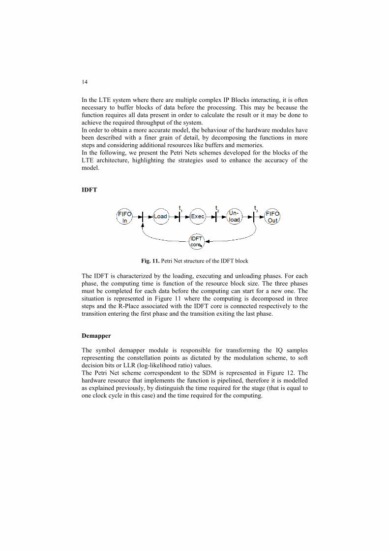
Fig. 11. Petri Net structure of the IDFT block
The IDFT is characterized by the loading, executing and unloading phases. For each
phase, the computing time is function of the resource block size. The three phases
must be completed for each data before the computing can start for a new one. The
situation is represented in Figure 11 where the computing is decomposed in three
steps and the R-Place associated with the IDFT core is connected respectively to the
transition entering the first phase and the transition exiting the last phase.
Demapper
The symbol demapper module is responsible for transforming the IQ samples
representing the constellation points as dictated by the modulation scheme, to soft
decision bits or LLR (log-likelihood ratio) values.
The Petri Net scheme correspondent to the SDM is represented in Figure 12. The
hardware resource that implements the function is pipelined, therefore it is modelled
as explained previously, by distinguish the time required for the stage (that is equal to
one clock cycle in this case) and the time required for the computing.

Timed Coloured Petri Nets for Performance Evaluation of DSP Applications: the 3GPP LTE
Case Study 15
Fig. 12. Petri Net structure for the Symbol demapper
The module operates with the granularity of a “complex data sample”, that for each
user is proportional to the number of resource blocks (in particular it is equal to the
number of resource blocks multiplied by the subcarriers sub and symbols per TTI
STTI). The first transition therefore generates the tokens corresponding to the data
samples that will be processed by the engine and put them in the input place. To
generate the next software task the processing of all the tokens must be terminated,
therefore a place representing a repository is used to activate the next software task
when the processing is finished. Some extra checks, that for simplicity are not shown
in the Figure, are used to guarantee the correct execution order.
Each sample generates a number of soft bits dependent on the modulation scheme
(represented by parameter Qm in the Figure). For each processed sample, the total
number of bits generated is updated, by the use of the place “count” that contains an
integer value token. The token is withdrawn and put back with its value updated. This
is an alternative to the use of many tokens representing the soft bits, that has been
chosen in order to increase the model efficiency. Indeed, for the simulation engine,
updating the value of a single token is simpler and quicker than maintaining all the
information related to a large number of tokens.
Rate De-Matcher
Fig. 13. Petri Net structure for the rate de-matcher
The rate de-matcher is activated when a request is ready and the symbol demapper
has produced enough bits to start the computation. Therefore, we use a condition on

16
the module input transition that checks if enough bits are available to start the
computation. In this case, the transition fires, with the effect that the number of bits is
updated and the computation is started. Figure 13 represents the corresponding net.
CTC (Turbo decoder)
The Turbo model has two input buffers, a core execution module and two output
buffers. The functioning is divided into 3 stages: loading, executing and unloading.
The corresponding PN is represented in Figure 14. The load operation can start when
the input port and a input buffer are available. After that, data are ready to be
processed by the core. The processing can start if an output buffer is available (to
write the produced data) and the execution core is free. At the end of the execution the
input buffer is freed and can be used to load new data. Finally data are unloaded when
an output port is available and at the end the output buffer is freed.
The transitions timing depends on the parameters affecting the system, and on the
configuration of the hardware module.
Fig. 14. Petri Net structure of the Turbo block
Experimental results
In order to collect information about the application performance, the Petri Net model
has been simulated using the CPNtool developed by CPN Group of University of
Aarhus in Denmark [19]. The tool allows to describe a TCPN, to automate the
simulations and to collect statistics. The results obtained from the model have been
compared with accurate simulation results obtained by implementing the application
on the reference architecture. These results have been collected by integrating the ISS
simulator of the Altera multithreaded CPU with software models of the hardware
event modules annotated with high level latencies.
In the following, we investigate different transmission scenarios. Each configuration
specifies the number of users, and for each user the assigned number of Resource
Blocks (RB), the coding rate (CR) and the modulation scheme. The number of users
and resource blocks affect the number of blocks processed by the system. The coding
rate and the modulation scheme affect the block dimension. In particular the block

Timed Coloured Petri Nets for Performance Evaluation of DSP Applications: the 3GPP LTE
Case Study 17
dimension increases with a lower coding rate and a modulation scheme with more
constellation points.
The considered scenarios are the following:
1. 110 users, with 1 resource block each, coding rate 5/6, modulation 64 QAM.
2. 5 users with different spectrum allocations: (RB=10,CR= 5/6), (RB=36,CR=1/9),
(RB=20,CR=1/9), (RB=4,CR=3/4), (RB=40, CR=1/4), modulation 64 QAM.
3. 2 users, with different spectrum allocations (RB=100,CR=5/6), (RB=10,CR=5/6),
modulation 64 QAM.
4. 50 users with 1 resource block each, coding rate 1/3, modulation QPSK.
5. 18 users with 6 resource blocks each, coding rate 2/3, modulation 16 QAM.
Figure 15 shows the data chunks output times obtained for in the five scenarios, for
both the simulations. The dimension and number of the data chunks elaborated for
each user are computed according to the LTE specification [18].
The performance evaluation shows that the system composed of the shaded blocks
represented in Figure 6 is able to support the strict timing performance (1ms for 110
resource blocks) in all the tested configurations. The use of the Petri Net model allows
to obtain such evaluation in early stages of the system development, without requiring
an actual hardware/software integration.

18
Fig. 15. Comparison between the system output times obtained through TCPN and the real
system simulation for different scenarios. Each colour represents a user.
The comparison with the results obtained by combining the hardware and software
modules shows that the TCPN model can provide a good accuracy. Figure 16
represents the errors in the arrival times for all the data chunks in all the five
scenarios. The difference between the arrival times obtained using the Petri Net and
the ones obtained simulating the system are always inferior to 35 microseconds, as
shown by the left Y-axis in the graph. Normalizing the values with the greatest arrival
time (first scenario) we obtain errors inferior to 5%, as shown by the right Y-axis in
the graph. Considering for each scenario a normalization to the greatest arrival time of
that scenario, we still obtain errors inferior to 5%.
0 100 200 300 400 500 600 700 800
TCPN
Sim.
0 100 200 300 400 500 600 700 800
TCPN
Sim.
0 100 200 300 400 500 600 700 800
TCPN
Sim.
0 100 200 300 400 500 600 700 800
TCPN
Sim.
Microseconds
0 100 200 300 400 500 600 700 800
TCPN
Sim.
a)
b)
c)
d)
e)

Timed Coloured Petri Nets for Performance Evaluation of DSP Applications: the 3GPP LTE
Case Study 19
0
5
10
15
20
25
30
35
1 6 11 16 21 26 31 36 41 46 51 56 61 66 71 76 81 86 91 96 101 106
Blocks
Mic
ros
ec
on
ds
0,00%
0,50%
1,00%
1,50%
2,00%
2,50%
3,00%
3,50%
4,00%
%E
rro
r
First Scenario Second Scenario Third Scenario Fourth Scenario Fifth scenario
Fig. 16. Absolute and percentage errors of the blocks arrival times in each scenario
Conclusion
One of the main problems, when designing a DSP application, is the meeting of strict
timing constraints; however, the verification of the system can usually be performed
very late in design phase. This paper proposes the use of Timed Coloured Petri Net
for the early evaluation of the system Performance of Hardware/Software DSP
applications. We show how to model an application by generating a TCPN that
considers the functions and the resources composing the system. The modelling of the
3GPP LTE application has been considered as case study. The experimental results
are quite accurate when compared with hardware/software simulations and, as a
substantial advantage, can be generated in early stages of the design, when
modifications and improvements of the system are still possible. The proposed
approach reduces the risk of highly expensive re-spins for the modification of the
final system and provides room for the exploration of the solution space.
References
1 D. D. Gajski, IP-based methodology, Proc. of 36th DAC, 1999.
2 C. Haubelt, J. Falk, J. Keinert, T. Schlichter, M. Streubühr, A. Deyhle, A. Hadert, J. Teich,
A SystemC-based design methodology for digital signal processing systems, EURASIP J.
Embedded Syst., 2007, n. 1.
3 K. Ueda, K. Sakanushi, Y. Takeuchi, M. Imai Architecture-level Performance Estimation
for IP-based Embedded Systems, DATE 2004.

20
4 A. Papoulis, Probability, Random Variables, and Stochastic Processes, McGraw-Hill, pp.
515-553, 1984.
5 B. D. Bunday, An Introduction to Queueing Theory, Oxford University Press, 1996.
6 W. M. Zubereck, Timed Petri Nets – definitions, properties and applications;
Microelectronic and Reliability, pp 627-644, 1991.
7 R. Zurawski, M. Zhou, Petri Nets and Industrial Applications: A Tutorial, IEEE
Transactions on industrial electronics, Vol. 41, N. 6, 1994.
8 A. Yakovlev, L. Gomes, Luciano Lavagno, Hardware Design and Petri Nets, Springer,
2000.
9 H. Blume, T. Von Sydow, T. G. Noll,A case Study for the application of Deterministic and
Stochastic Petri Nets in SoC communication Domain, Journal of VLSI Signal Processing,
2006.
10 J. Zhan, N. Sang, G. Xiong, Formal Co-verification for SoC Design with Colored Petri Net,
Lecture Notes in Computer Science, 2005.
11 P. Maciel, E. Barros, W. Rosenstiel, A Petri Net Model for Hardware/Software Codesign,
Design Automation for Embedded Systems Journal, Springer 1999.
12 C. Rust, J. Tacken, C. B¨oke, Pr/T-Net Based Seamless Design of Embedded Real-Time
Systems, ATPN 2001.
13 L. Gomes, A. Costa, Petri nets as supporting formalism within Embedded Systems Co-
design, Industrial Embedded Systems Symposium, 2006.
14 C. A. Petri, Communication with Automatas, PhD Dissertation, University of Bonn, 1962
(in German).
15 K. Jensen, Coloured Petri Nets. Basic Concepts, Analysis Methods and Practical Use.
Volume 1, Basic Concepts. Monographs in Theoretical Computer Science, Springer-Verlag,
1997.
16 M. Bourcerie, J. Y. Morel, Algebraically structured colored Petri nets to model sequential
processes. IEEE Transactions on Systems, Man, and Cybernetics 27 (4): 681-6, 1997.
17 3GPP TS 36.300 Technical Specification group radio Access Network, E-UTRA, E-
UTRAM, Overall Description, Stage 2
18 3GPP TS 36.201, 36.211-14
19 CPN Tools, Coloured Petri Net Group, University of Aarhus,
Denmark,www.daimi.au.dk/CPnets/
20 Altera Corporation,
21 R2-061402, Concept evaluation of user plane latency in LTE, Ericsson.
www.altera.com
22 R2-072187, LS on LTE latency analysis, Ericsson.