the practitioner’s guide to coloured petri nets filesoftware tools for technology transfer...
TRANSCRIPT

Software Tools for Technology Transfer manuscript No.(will be inserted by the editor)
The Practitioner’s Guide to Coloured Petri NetsLars M. Kristensen, Søren Christensen, Kurt Jensen
CPN Group, Department of Computer Science, University of Aarhus, Denmark;e-mail: flmkristensen,schristensen,[email protected]
Abstract. Coloured Petri Nets (CP-nets or CPNs) provide aframework for design, specification, validation, and verifica-tion of systems. CP-nets have a wide range of application ar-eas and many CPN projects have been carried out in industry,e.g., in the areas of communication protocols, operating sys-tems, hardware designs, embedded systems, software systemdesigns, and business process re-engineering.
Design/CPN is a graphical computer tool supporting thepractical use of CP-nets. The tool supports construction, sim-ulation, functional, and performance analysis of CPN models.The tool is used by more than four hundred organisations inforty different countries – including one hundred commercialcompanies. It is available free of charge, also for commercialuse.
This paper provides a comprehensive road map to thepractical use of CP-nets and the Design/CPN tool. We givean informal introduction to the basic concepts and ideas un-derlying CP-nets. The key components and facilities of theDesign/CPN tool are presented and their use illustrated. Thepaper is self-contained and does not assume any prior knowl-edge of Petri nets and CP-nets nor any experience with theDesign/CPN tool.
Key words: High-level Petri Nets – Coloured Petri Nets –Practical Use – Modelling – Validation – Verification – Visu-alisation – Tool Support.
1 Introduction
An increasing number of system development projects areconcerned with distributed and concurrent systems. There arenumerous examples, ranging from large scale systems, in theareas of telecommunication and applications based on WWWtechnology, to medium or small scale systems, in the area ofembedded systems.
The development of concurrent and distributed systemsis complex. A major reason is that the execution of such sys-tems may proceed in many different ways, e.g., dependingon whether messages are lost, the speed of the processes in-volved, and the time at which input is received from the envi-ronment. As a result, distributed and concurrent systems are,by nature, complex and difficult to design and test.
Coloured Petri Nets (CP-nets or CPNs) [24–27] providea framework for construction and analysis of distributed andconcurrent systems. A CPN model of a system describes thestates which the system may be in and the transitions betweenthese states. CP-nets have been applied in a wide range ofapplication areas and many projects have been carried outin industry [26] and documented in the literature, e.g., inthe areas of communication protocols [16,21], audio/videosystems [8], operating systems [6,7], hardware designs [17,45], embedded systems [43], software system designs [33,44], and business process re-engineering [35,40].
The development of CP-nets has been driven by the desireto develop an industrial strength modelling language – at thesame time theoretically well-founded and versatile enough tobe used in practice for systems of the size and complexityfound in typical industrial projects. To achieve this, we havecombined the strength of Petri nets [36] with the strengthof programming languages. Petri nets provide the primitivesfor describing synchronisation of concurrent processes, whileprogramming languages provide the primitives for definingdata types and manipulating data values.
CPN models can be structured into a number of relatedmodules. This is particularly important when dealing withCPN models of large systems. The module concept of CP-nets is based on a hierarchical structuring mechanism, whichsupports a bottom-up as well as top-down working style. Newmodules can be created from existing modules, and modulescan be reused in several parts of the CPN model. By means ofthe structuring mechanism it is possible to capture differentabstraction levels of the modelled system in the same CPNmodel. A CPN model which represents a high level of ab-
2 Lars M. Kristensen et al.: The Practitioner’s Guide to Coloured Petri Nets
straction is typically made in the early stages of design oranalysis. This model is then gradually refined to yield a moredetailed and precise description of the system under consid-eration.
CPN models are executable. This implies that it is pos-sible to investigate the behaviour of the system by makingsimulations of the CPN model. Very often, the goal of do-ing simulations is to debug and validate the system design.However, simulations can equally well serve as a basis forinvestigating the performance of the considered system.
Visualisation is a technique which is closely related tosimulation of CPN models. Observation of every single stepin a simulation is often too detailed a level of observing thebehaviour of a system. It provides the observer with an over-whelming amount of detail, particularly for very large CPNmodels. By means of high level visual feedback from simu-lations, information about the execution of the system can beobtained at a more adequate level of detail. Another impor-tant application of visualisation is the possibility of present-ing design ideas and results using application domain con-cepts. This is particularly important in discussions with peo-ple and colleagues unfamiliar with CP-nets.
Time plays a significant role in a wide range of distributedand concurrent systems. The correct functioning of many sys-tems crucially depends on the time taken up by certain activi-ties, and different design decisions may have a significant im-pact on the performance of a system. CP-nets includes a timeconcept which makes it possible to capture the time takenby different activities in the system. Timed CPN models andsimulation can be used to analyse the performance of a sys-tem, e.g., investigate the quality of service (e.g., delay) or thequantity of service (e.g., throughput) provided by the system.
The state space method of CP-nets makes it possible tovalidate and verify the functional correctness of systems. Thestate space method relies on the computation of all reach-able states and state changes of the system. By means ofa constructed state space, behavioural properties of the sys-tem can be verified. Examples of such properties are the ab-sence of deadlocks in the system, the possibility of alwaysreaching a given state, and the guaranteed delivery of a givenservice. The state space method of CP-nets can also be ap-plied to timed CP-nets. Hence, it is also possible to investi-gate the functional correctness of systems modelled by meansof timed CP-nets.
Design/CPN [9,37] is a graphical computer tool support-ing CP-nets. It consists of three closely integrated compo-nents. The CPN editor supports construction and editing ofhierarchical CPN models. Simulation of CPN models is sup-ported by the CPN simulator, while the CPN state space toolsupports the state space method of CP-nets. In addition tothese three main components, the tool includes a number ofadditional packages and libraries. One of these is a set ofpackages, which supports visualisation by means of businesscharts, message sequence charts (MSC), and construction ofapplication specific graphics.
The Design/CPN tool is used by more than four hundredorganisations in forty different countries – including one hun-
dred commercial companies. It is available free of charge,also for commercial use. More than 50 man-years have beeninvested in the development of CP-nets and Design/CPN.
CP-nets has been developed over the last 20 years. Theprime entrepreneur has been the CPN group at University ofAarhus, Denmark, headed by Kurt Jensen. We have devel-oped the basic model, including the use of data types and hi-erarchy constructs. We have defined the basic concepts suchas the dynamic properties and developed the theory behindmany of the existing analysis methods. Together with MetaSoftware Corporation [13], we have played a key role in thedevelopment of high-quality tools supporting the use of CP-nets. Finally, we have been engaged in a large number of ap-plication projects, many of these in industrial settings. Formore information on the group and its work see [20]. Moredetailed acknowledgements of some of the individual contri-butions during the first 15 years can be found in the prefacesof [24–26].
Outline. This paper is organised as follows. Section 2 givesan informal introduction to the syntax and dynamic behaviourof CP-nets. In this section, we also introduce the hierarchicalstructuring mechanism of CP-nets. Section 3 gives an over-view of the Design/CPN tool. Section 4 explains how theconstruction of CPN models is supported by the CPN edi-tor. Section 5 considers simulation of CPN models and theCPN simulator. Section 6 presents the packages supportingvisualisation and gives some examples of their use. Section 7introduces the time concept of CP-nets and explains how thiscan be used to conduct simulation based performance analy-sis of systems. Section 8 introduces the CPN state space tooland the state space method of CP-nets. Section 9 sums up theconclusions and explains how to get started using CP-netsand the Design/CPN tool.
2 Coloured Petri Nets
This section gives an informal introduction to the syntax andsemantics of CP-nets. A small communication protocol isused throughout the section to illustrate the basic conceptsof the CPN language. Later, the communication protocol willalso be used to introduce the time concept and the state spacemethod of CP-nets.
One should keep in mind that it is very difficult (probablyimpossible) to give an informal explanation which is totallycomplete and unambiguous. Thus it is extremely importantfor the soundness of the CPN modelling language and the De-sign/CPN tool that the informal description is complementedby a more formal definition. The formal definition of the syn-tax and semantics of CP-nets can be found in [24,22]. For thepractical use of CP-nets and Design/CPN, however, it sufficesto have an intuitive understanding of the syntax and seman-tics. This is analogous to programming languages, which aresuccessfully applied by users even though they are unfamiliarwith the formal, mathematical definitions of the languages.

Lars M. Kristensen et al.: The Practitioner’s Guide to Coloured Petri Nets 3
Send
PacketBuffer
SenderHS Sender#4
ReceiverHS Receiver#5
Communication ChannelHS ComChannel#3
Received
PacketBuffer
TransmitData
Frame
ReceiveAck
Frame
TransmitAck
Frame
ReceiveData
Frame
Fig. 1. Stop-and-wait communication protocol.
2.1 Example: A Communication Protocol
We consider a stop-and-wait protocol from the datalink con-trol layer of the OSI network architecture. The protocol istaken from [2]. The stop-and-wait protocol is quite simple,and does not in any way represent a sophisticated protocol.However, the protocol is interesting enough to deserve closerinvestigation, and it is also complex enough for introducingthe basic constructs of CP-nets.
Figure 1 gives an overview of the protocol considered.The system consists of a Sender (left) transmitting data pack-ets to a Receiver (right). The data packets to be transmittedare located in a Send buffer at the sender side. Communica-tion with the receiver takes place on a bidirectional Commu-nication Channel (bottom).
The data packets have to be delivered exactly once andin the correct order into the Received buffer at the receiverside. Obtaining this service is complicated by the fact that thesender and receiver communicate via an unreliable communi-cation channel, i.e., packets may be lost during transmissionand packets may overtake each other. One way of achievingthe desired service is to use a so-called stop-and-wait retrans-mission strategy. The idea is that the sender keeps sendingthe same data packet until a matching acknowledgement isreceived, in which case the next data packet can be transmit-ted. For simplicity, this particular stop-and-wait protocol usesan unlimited number of retransmissions.
The sender sends a data packet on the communicationchannel by constructing a data frame and putting the dataframe in the TransmitData frame buffer. A data frame is apair consisting of a sequence number and a data packet. Thechannel will then attempt to transmit the data frame, and, ifsuccessful, the data frame will be delivered into the Receive-Data frame buffer, where it can be processed by the receiver.The receiver delivers data packets to the upper protocol layersusing the data packet buffer Received. The protocol uses se-quence numbers to be able to match acknowledgements anddata packets, i.e., to be able to deduce which acknowledge-ments correspond to which data packets, and to be able to de-duce whether a given data packet has already been received.
The receiver sends an acknowledgement for a receiveddata frame by constructing an acknowledgement frame and
putting it in the TransmitAck frame buffer. An acknowledge-ment frame consists of a sequence number indicating the se-quence number of the data packet that the receiver expectsnext. Similar to data frames, the channel will then attempt totransmit it, and, if successful, it will turn up in the ReceiveAckframe buffer at the sender side, where it can be processed bythe sender.
We will return to the inscriptions placed next to the el-lipses and in the upper left corner of the boxes later in thissection.
2.2 Modelling of States
Petri nets are, in contrast to most specification languages,state and action oriented at the same time, providing an ex-plicit description of both the states and the actions of the sys-tem. This means that, at a given moment, the modeller candetermine freely whether to concentrate on states or on ac-tions.
A CP-net is always created as a graphical drawing. Fig-ure 2 shows the CP-net that models the sender in the stop-and-wait protocol. It consists of two parts. The part on theleft models the sending of data frames, the part on the rightmodels the reception of acknowledgement frames.
Places. The states of a CP-net are represented by means ofplaces (which are drawn as ellipses or circles). The sender ismodelled using six different places. By convention, we writethe names of the places inside the ellipses. The names haveno formal meaning – but they have huge practical importancefor the readability of a CP-net (just like the use of mnemonicnames in traditional programming). A similar remark appliesto the graphical appearance of the places, i.e., the line thick-ness, size, colour, font, position, etc.
The place Send (top left) models the data packet buffer,containing the data packets which the sender has to trans-mit to the receiver. The places TransmitData and ReceiveAck(at the bottom) model the frame buffers between the senderand the communication channel. The place NextSend (mid-dle) models the internal status of the sender – it will keeptrack of the sequence number of the data packet to be sentnext, and it will indicate whether an acknowledgement hasbeen received for the data packet which is currently beingtransmitted. The places Sending and Waiting model the twopossible positions of the control flow in the sender – eitherthe sender is just about to start Sending a data frame, or thesender is Waiting after having sent a data frame.
Types. Each place has an associated type (colour set) deter-mining the kind of data that the place may contain. By con-vention, the type of a place is written in italics, to the lowerleft or right of the place. The types are similar to types in aprogramming language. The types of a CP-net can be arbitrar-ily complex, e.g., a record where one field is a real, anothera text string and a third a list of integers. Figure 3 shows thetype definitions used in the stop-and-wait protocol.

4 Lars M. Kristensen et al.: The Practitioner’s Guide to Coloured Petri Nets
ReceiveAckFrame
P InTransmitDataFrame
P Out
SendPacketBuffer
P I/O
ReceiveAckFrameAccept
Waiting
DataFrame
1‘(0,"")
TimeOut
NextSend
SeqxStatus
SendDataFrame
SendingDataFrame
ackframe rn
(sn,p)
dframe
dframe
p::packets
(sn,acked)
(sn,status)
if (rn > sn)then (rn,acked)else (sn, status)
(sn,notacked)
packets
dframe
dataframe dframe
dframe
dframe
(sn,notacked)
Fig. 2. Sender of the stop-and-wait protocol.
(� —– data packets —– �)color Packet = string ;color PacketBuffer = list Packet ;
(� —– status and sequence numbers —– �)color Seq = int ;color Status = with acked j notacked ;
color SeqxStatus = product Seq � Status ;
(� —– data and acknowledgement frames —– �)color DataFrame = product Seq � Packet ;color AckFrame = Seq ;
color Frame = uniondataframe : DataFrame + ackframe : AckFrame ;
Fig. 3. Type (colour set) definitions.
We use eight different types to model the sender. Theplace Send has the type PacketBuffer. This type is definedas a list of Packets representing the possible contents of thepacket buffer modelled by the place Send. The type Packet isdefined as a string denoting the set of text strings. The type ofthe place NextSend is SeqxStatus. This type is defined as theproduct (or pair) of the types Seq and Status. The type Seq isdefined as int (integers), and Status is defined as an enumera-tion type containing two possible values: acked and notacked.Hence, the type SeqxStatus contains all pairs in which thefirst component is an integer (denoting a sequence number)and the second component is either acked or notacked (in-dicating whether an acknowledgement has been received forthe data packet currently being sent).
The places Sending and Waiting have the type DataFrame,which is defined as a product of Sequence numbers and Pack-ets. The places TransmitData and ReceiveAck both have thetype Frame, which is defined as the union of type DataFrameand type AckFrame. The type AckFrame is simply a Sequencenumber.
Markings. A state of a CP-net is called a marking. It con-sists of a number of tokens positioned (distributed) on theindividual places. Each token carries a value (colour), whichbelongs to the type of the place on which the token resides.The tokens that are present on a particular place are calledthe marking of that place. For historical reasons, we some-times refer to token values as token colours, in the same wayas we refer to data types as colour sets. This is a metaphoricpicture where we consider the tokens of a CP-net to be distin-guishable from each other and hence “coloured” – in contrastto low-level Petri nets which have “black” indistinguishabletokens.
The marking of a place is, in general, a multi-set of tokenvalues. A multi-set is similar to a set, except that there maybe several appearances of the same element. This means thata place may have several tokens with the same token value.As an example, a possible marking of the place TransmitDatais the following:
2‘dataframe(0,”CP-nets”) + 4‘dataframe(1,”CPN”)
This marking contains two tokens with value dataframe-(0,”CP-nets”) and four tokens with value dataframe(1,”CPN”).By convention, multi-sets are written as a sum (+) using thesymbol prime (‘) (pronounced “of”) to denote the number ofappearances of an element.

Lars M. Kristensen et al.: The Practitioner’s Guide to Coloured Petri Nets 5
Initial marking. A CP-net has a distinguished marking – theinitial marking, which is used to describe the initial state ofthe system. The initial marking of a place is, by convention,written on the upper left or right of the place. The place Sendhas an initial marking consisting of a single token with thevalue [”Software”,” Tools f”,”or Techn”,”ology Tr”,”ansfer. ”], i.e.,a list of five packets. The place NextSend initially contains asingle token with the value (0,acked), denoting that the packetto be sent first will be assigned sequence number 0, and thatan acknowledgement has been received for the previous datapacket (since initially there is no previous packet). Initiallythe sender is in state waiting, as indicated by the initial mark-ing of the place Waiting. Initially, the remaining three placescontain no tokens. The specification of the initial marking istherefore (by convention) omitted for these three places.
2.3 Modelling of Actions
Transitions. The actions of a CP-net are represented by me-ans of transitions (which are drawn as rectangles). As withplaces, we write the name of the transitions inside the rect-angles. The sender consists of four transitions. The transitionAccept models the action taken when the next data packetis accepted for transmission. The transition SendDataFramemodels the sending of a data frame, and ReceiveAckFramemodels the reception of an acknowledgement frame. Time-Out is used to model the occurrence of a timeout so that thedata frame can be retransmitted.
Arcs and arc expressions. Transitions and places are con-nected by arcs. The actions of a CP-net consist of occur-rences of transitions. An occurrence of a transition removestokens from places connected to incoming arcs (input places),and adds tokens to places connected to outgoing arcs (outputplaces), thereby changing the marking (state) of the CP-net.This is also referred to as the token game. As an example, thetransition Accept has three incoming arcs and three outgoingarcs. Hence, an occurrence of this transition will remove to-kens from the places Waiting, Send, and NextSend, and addtokens to the places Sending, Send, and NextSend.
The exact number of tokens added and removed by theoccurrence of a transition, and their data values are deter-mined by the arc expressions, which are positioned next tothe arcs. How to determine the values of the tokens removedand added will be explained in the next subsection. A dou-ble arc, like the dashed arc between TimeOut and NextSend,is a shorthand for two opposite directed arcs with identicalarc expressions. As we will see in the next section, an actionof a CP-net consists, in general, of one or more transitionsoccurring concurrently.
2.4 Dynamic Behaviour
We now describe the dynamic behaviour (operational seman-tic) of CP-nets. That is, the conditions under which transitionsmay occur, and the effect of an occurrence of a transition onthe marking of the CP-net.
(� —– data packets —– �)var p : Packet ;var packets : PacketBuffer ;
(� —– status and sequence numbers —– �)var sn,rn : Seq ;var status : Status ;
(� —– data frames —– �)var dframe : DataFrame ;
Fig. 4.Variable declarations for the stop-and-wait protocol
p ”Software”packets [” Tools f”,”or Techn”,”ology Tr”,”ansfer. ”]
sn 0dframe (0,””)
Fig. 5. A binding of transition Accept.
Variables and bindings. To talk about an occurrence of atransition, we need to assign (bind) data values to the (free)variables occurring in the arc expressions on the surroundingarcs of the transition. Otherwise, it is impossible to evalu-ate the arcs expressions. The transition Accept has four vari-ables: p of type Packet, packets of type PacketBuffer, sn oftype Seq, and dframe of type DataFrame. The variable dec-larations, specifying the variables and their types, are shownin Fig. 4. Variables can be assigned data values belonging tothe type of the variable.
Let us now assume that we assign data values to the vari-ables of the transition Accept by creating the binding listed inFig. 5, where should be read ”bound to”.
Figure 6 shows, for each surrounding arc of Accept, themulti-set of tokens resulting from evaluating the correspond-ing arc expressions in the binding listed in Fig. 5. In this caseall multi-sets contain a single token. For all arc expressions,the result is straightforward. The only exception is the arc ex-pression p::packets on the incoming arc from Send. The infixoperator :: is the basic list constructor. This means that theresult of evaluating the expression p::packets in the bindingof Fig. 5 is the list obtained by inserting the value ”Software”,bound to p, at the front of the list bound to packets.
Figure 6 also shows the initial marking of the places sur-rounding the transition Accept. The marking of each place isindicated next to the place. The number of tokens on the placeis shown in the small circle, while the detailed token valuesare indicated in the dashed box next to the small circle.
A binding of a transition is also written in the form:hv1 = d1; v2 = d2; : : : vn = dni where vi for i 2 1::n isa variable, and di is the value assigned to vi. As an example,the binding in Fig. 5 can be written as:
h p = ”Software”, sn = 0, dframe = (0,””),packets = [” Tools f”,”or Techn”,”ology Tr”,”ansfer. ”] i
In addition to the arc expressions, it is possible to attacha boolean expression (with variables) to each transition. The

6 Lars M. Kristensen et al.: The Practitioner’s Guide to Coloured Petri Nets
SendingDataFrame
Accept
SendPacketBuffer
1 1‘["Software"," Tools f","or Techn","ology tr","ansfer. "]
Waiting
DataFrame
1 1‘(0,"")
NextSendSeqxStatus
1 1‘(0,acked)
(sn,p)
1‘(0,"Software")
dframe1‘(0,"")
p::packets
1‘["Software"," Tools f","or Techn","ology tr","ansfer. "]
(sn,acked)
1‘(0,acked)
(sn,notacked)
1‘(0,notacked)
packets
1‘[" Tools f","or Techn","ology tr","ansfer."]
Fig. 6.Evaluation of arc expressions for Accept.
boolean expression is called a guard. It specifies that we onlyaccept bindings for which the boolean expression evaluatesto true. However, none of the transitions of the sender uses aguard.
Enabling. In order for a transition to be enabled in a mark-ing, i.e., ready to occur, it must be possible to bind (assign)data values to the variables appearing on the surrounding arcexpressions and in the guard of the transition such that: 1)each of the arc expressions evaluate to tokens which are pre-sent on the corresponding input place, and 2) the guard (ifany) is satisfied.
Figure 6 tells us that an occurrence of the transition Ac-cept (with the binding in Fig. 5) removes a token with value(0,””) from the place Waiting, a token with value [”Software”,”Tools f”, ”or Techn”,”ology Tr”,”ansfer. ”] from the place Send,and a token with value (0,acked) from the place NextSend.
This binding of Accept is enabled in the initial marking,since the tokens to which the arc expressions evaluate arepresent on the corresponding input places.
Obviously, there are many other bindings that we may tryfor the transition Accept in the initial marking. However, noneof these are enabled in the initial marking. This can be seenas follows. The place Send has only one token. Hence weneed to bind p to the head of the list, and packets to the tail ofthe list. The place NextSend also contains a single token withvalue (0,acked). Hence, we need to bind sn to 0. The placeWaiting also contains a single token with value (0,””), hencewe need to bind dframe to this value. Therefore the enabledbinding is uniquely determined by the tokens residing on theinput places.
The possible bindings of data values to the variables of atransition correspond to the possible ways in which a transi-tion can occur. However, as we demonstrated above, only asubset of these will, in general, be enabled in a given mark-ing.
Occurrence. The occurrence of a transition in an enabledbinding removes tokens from the input places and adds tokensto the output places of the transition. The values of the tokensremoved from an input place are determined by evaluating the
Waiting
DataFrame
Accept
SendingDataFrame
1 ‘(0,"Software")
NextSend
SeqxStatus
1 1‘(0,notacked)
SendPacketBuffer
1 1‘[" Tools f","or Techn","ology tr","ansfer. "]
(sn,p)
dframe
p::packets
(sn,acked)
(sn,notacked)
packets
Fig. 7. Marking resulting from the occurrence of Accept.
arc expression on the corresponding input arc. Similarly, thevalues of tokens added to an output place are determined byevaluating the arc expression on the corresponding output arc(see Fig. 6). Figure 7 shows the marking of the surroundingplaces of the transition Accept resulting from the occurrenceof this transition in the initial marking with the enabled bind-ing listed in Fig. 5.
Hence, the occurrence of the transition Accept has the ef-fect that the data packet at the head of the list, residing on theplace Send, is removed. The status of the sender, modelled byNextSend, is updated so that the token, residing on NextSend,indicates that an acknowledgement has not yet been received(notacked) for the data packet, which is now being transmit-ted. The control flow of the sender is changed from being inthe state waiting to sending, by removing the token, corre-sponding to the data frame previously being transmitted fromthe place Waiting, and adding a token to the place Sendingcorresponding to the newly constructed data frame, which isnow being transmitted.
We now briefly sum up the remaining parts of the CP-netin Fig. 2. The transition TimeOut is enabled when the dataframe currently being sent is on Waiting, and an acknowl-edgement has not yet been received (status is notacked) forthe data frame currently being sent. An occurrence of Time-Out changes the control in the sender from being waiting tosending, by removing the data frame on Waiting and addingit to the place Sending so that it can be retransmitted. At firstglance, it may seem strange that we do not specify the condi-tions under which retransmissions occur. However, for a lotof purposes this is not necessary. Most CP-nets are used toinvestigate the logical and functional correctness of a sys-tem design. For this purpose it is often sufficient to describethat retransmissions may appear, e.g., because the communi-cation channel is slow. However it may not be necessary, oreven beneficial, to consider how often this happens – the pro-tocol must be able to cope with all kinds of communicationchannels, both those which work so well that there are noretransmissions and those in which retransmissions are fre-quent. Later on we will see that CP-nets can be extended witha time concept that allows to describe the duration of the in-dividual actions and states. This will permit to investigate the
Lars M. Kristensen et al.: The Practitioner’s Guide to Coloured Petri Nets 7
performance of the modelled system, i.e., how fast and ef-fectively it operates. Then we will give a much more precisedescription of retransmissions (e.g., that they occur when noacknowledgement has been received inside two hundred mil-liseconds).
The reception of acknowledgement frames is modelledby ReceiveAckFrame. The occurrence of this transition re-moves an acknowledgement frame from the place Receive-Ack and compares the sequence number rn in the acknowl-edgement frame with the sequence number sn of the dataframe currently being sent. If the sequence number in the ac-knowledgement is greater than the sequence number of thedata frame currently being sent (recall that the receiver sendsthe sequence number of the data frame it expects next), thenthe sequence number of the next data packet is updated, andthe acknowledgement status is changed to indicate that anacknowledgement has been received for the data frame cur-rently being sent. This is accomplished by the if-then-elseconstruction used on the arc from ReceiveAckFrame to Next-Send, which puts a token on NextSend with a value accordingto the above description.
Occurrence sequences and steps. An execution of a CP-netis described by means of an occurrence sequence. It specifiesthe markings that are reached and the steps that occur. Above,we have seen an occurrence sequence of length one. It con-sisted of a single step, the occurrence of Accept in the bindingin Fig. 5 in the initial marking, and leading to the marking inFig. 7.
In this marking, the transition SendDataFrame is enabledin a binding in which the variable dframe is assigned the value(0,”Software”). Hence, the occurrence sequence can be contin-ued with a step corresponding to the occurrence of this bind-ing of SendDataFrame. This leads to a new marking in whichthe marking of Send and ReceiveAck remains unchanged,one token with value dataframe(0,”Software”) is on Transmit-Data (corresponding to the data frame being placed in theTransmitData buffer for transmission), and one token withvalue (0,”Software”) is on Waiting.
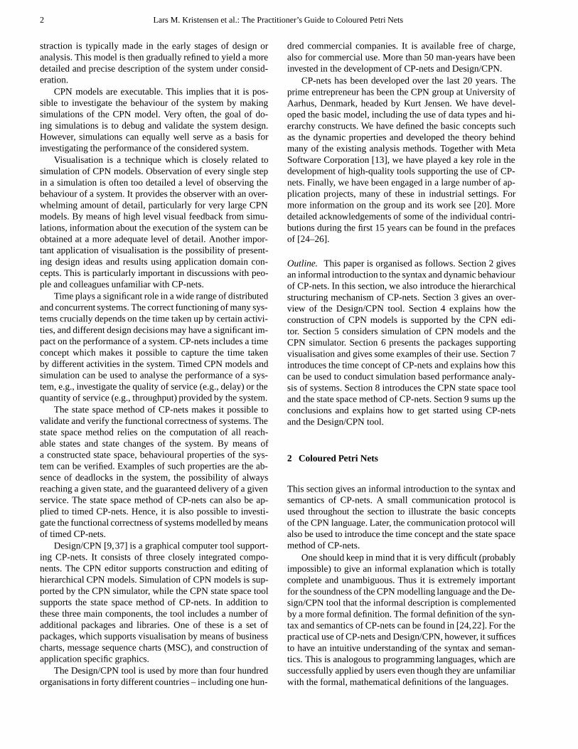
In general, a step may consist of several enabled bindingelements occurring concurrently. A binding element is a pairconsisting of a transition and a binding of its variables. As anexample, consider the marking of the sender shown in Fig. 8.This marking is identical to the marking reached after the oc-currence of Accept in the initial marking, except that two to-kens are residing on the place ReceiveAck; one token withvalue ackframe(0), and one token with value ackframe(1). Inthis marking, the three binding elements listed below are en-abled.
1. (SendDataFrame; hdframe = (0,”Software”)i)2. (ReceiveAckFrame; hrn = 0; sn = 0; status = ackedi)3. (ReceiveAckFrame; hrn = 1; sn = 0; status = ackedi)
The binding elements 1 and 2 are concurrently enabled,since each binding element can get those tokens that it needs(i.e., those specified by the input arc expressions) – withoutsharing the tokens with the other binding element. The same
is true for the binding elements 1 and 3. However, the bind-ing elements 2 and 3 are not concurrently enabled, since theycannot both get the only (0,acked) token on NextSend. Thesetwo binding elements are in conflict.
In general, it is possible for a transition to be concurrentlyenabled with itself (using two different bindings or using thesame binding twice). Hence, a step, from one marking to thenext, may involve a multi-set of binding elements. The mark-ing, resulting from the occurrence of a step consisting of sev-eral binding elements, is the same as the marking reached bythe occurrence of the individual binding elements in some ar-bitrary order. This marking is well-defined since it is a funda-mental property of Petri nets that the marking, resulting fromthe occurrence of a multi-set of concurrently enabled bindingelements, is independent of the order in which the individualbinding elements occur.
A finite occurrence sequence is an occurrence sequenceconsisting of a finite number of markings and steps. An infi-nite occurrence sequence is an occurrence sequence consist-ing of an infinite number of markings and steps. An infiniteoccurrence sequence corresponds to a non-terminating exe-cution of the system.
2.5 Hierarchical CP-nets
The basic idea underlying hierarchical CP-nets is to allowthe modeller to construct a large model by using a number ofsmall CP-nets like the one in Fig. 2. These small CP-nets arecalled pages. These pages are then related to each other in awell-defined way as explained below. This is similar to thesituation in which a programmer constructs a large programby means of a set of modules. Many CPN models consist ofmore than one hundred pages with a total of many hundredplaces and transitions. Without hierarchical structuring facil-ities, such a model would have to be drawn as a single (verylarge) CP-net, and it would become totally incomprehensible.
In the previous section, we described a CPN model for thesender. In this section we describe models for the receiver andthe communication channel, and we show how these threesubmodels can be put together to form a model of the entirestop-and-wait protocol.
In a hierarchical CP-net, it is possible to relate a transition(and its surrounding arcs and places) to a separate CP-net,providing a more precise and detailed description of the ac-tivity represented by the transition. The idea is analogous tothe hierarchy constructs found in many graphical descriptionlanguages (e.g., data flow and SADT diagrams). It is also,in some respects, analogous to the module concepts found inmany modern programming languages. At one level, we wantto give a simple description of the modelled activity with-out having to consider internal details about how it is carriedout. At another level, we want to specify the more detailedbehaviour. Moreover, we want to be able to integrate the de-tailed specification with the more crude description – and thisintegration must be done in such a way that it becomes mean-ingful to speak about the behaviour of the combined system.
8 Lars M. Kristensen et al.: The Practitioner’s Guide to Coloured Petri Nets
ReceiveAckFrame
P In
2 1‘ackframe(0)+1‘ackframe(1)TransmitData
Frame
P Out
SendPacketBuffer
P I/O
1 1‘[" Tools f","or Techn","ology tr","ansfer. "]
ReceiveAckFrameAccept
Waiting
DataFrame
1‘(0,"")
TimeOut
NextSend
SeqxStatus
1 1‘(0,acked)
SendDataFrame
SendingDataFrame
1 1‘(0,"Software")
ackframe rn
(sn,p)
dframe
dframe
p::packets
(sn,acked)
(sn,status)
if (rn > sn)then (rn,acked)else (sn, status)
(sn,notacked)
packets
dframe
dataframe dframe
dframe
dframe
(sn,notacked)
Fig. 8.Marking of the sender.
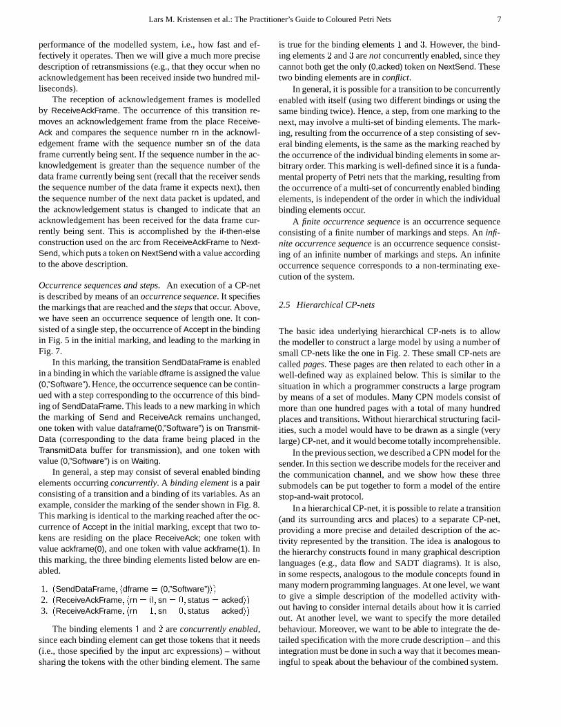
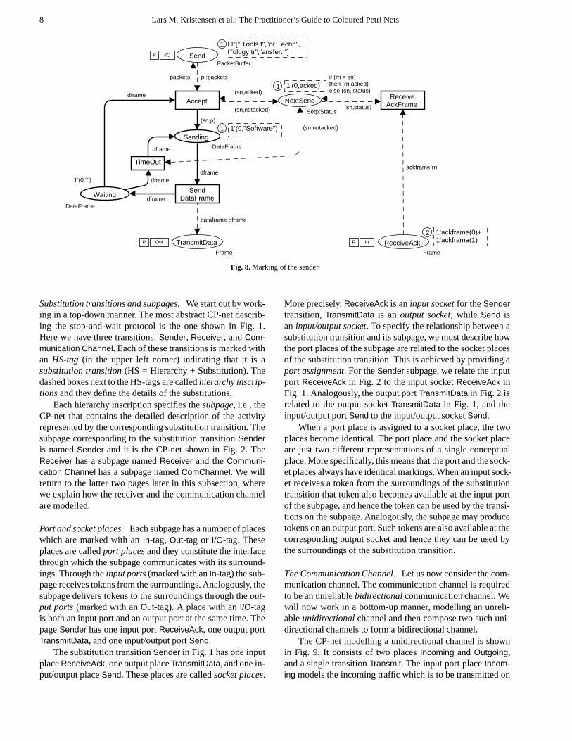
Substitution transitions and subpages. We start out by work-ing in a top-down manner. The most abstract CP-net describ-ing the stop-and-wait protocol is the one shown in Fig. 1.Here we have three transitions: Sender, Receiver, and Com-munication Channel. Each of these transitions is marked withan HS-tag (in the upper left corner) indicating that it is asubstitution transition (HS = Hierarchy + Substitution). Thedashed boxes next to the HS-tags are called hierarchy inscrip-tions and they define the details of the substitutions.
Each hierarchy inscription specifies the subpage, i.e., theCP-net that contains the detailed description of the activityrepresented by the corresponding substitution transition. Thesubpage corresponding to the substitution transition Senderis named Sender and it is the CP-net shown in Fig. 2. TheReceiver has a subpage named Receiver and the Communi-cation Channel has a subpage named ComChannel. We willreturn to the latter two pages later in this subsection, wherewe explain how the receiver and the communication channelare modelled.
Port and socket places. Each subpage has a number of placeswhich are marked with an In-tag, Out-tag or I/O-tag. Theseplaces are called port places and they constitute the interfacethrough which the subpage communicates with its surround-ings. Through the input ports (marked with an In-tag) the sub-page receives tokens from the surroundings. Analogously, thesubpage delivers tokens to the surroundings through the out-put ports (marked with an Out-tag). A place with an I/O-tagis both an input port and an output port at the same time. Thepage Sender has one input port ReceiveAck, one output portTransmitData, and one input/output port Send.
The substitution transition Sender in Fig. 1 has one inputplace ReceiveAck, one output place TransmitData, and one in-put/output place Send. These places are called socket places.
More precisely, ReceiveAck is an input socket for the Sendertransition, TransmitData is an output socket, while Send isan input/output socket. To specify the relationship between asubstitution transition and its subpage, we must describe howthe port places of the subpage are related to the socket placesof the substitution transition. This is achieved by providing aport assignment. For the Sender subpage, we relate the inputport ReceiveAck in Fig. 2 to the input socket ReceiveAck inFig. 1. Analogously, the output port TransmitData in Fig. 2 isrelated to the output socket TransmitData in Fig. 1, and theinput/output port Send to the input/output socket Send.
When a port place is assigned to a socket place, the twoplaces become identical. The port place and the socket placeare just two different representations of a single conceptualplace. More specifically, this means that the port and the sock-et places always have identical markings. When an input sock-et receives a token from the surroundings of the substitutiontransition that token also becomes available at the input portof the subpage, and hence the token can be used by the transi-tions on the subpage. Analogously, the subpage may producetokens on an output port. Such tokens are also available at thecorresponding output socket and hence they can be used bythe surroundings of the substitution transition.
The Communication Channel. Let us now consider the com-munication channel. The communication channel is requiredto be an unreliable bidirectional communication channel. Wewill now work in a bottom-up manner, modelling an unreli-able unidirectional channel and then compose two such uni-directional channels to form a bidirectional channel.
The CP-net modelling a unidirectional channel is shownin Fig. 9. It consists of two places Incoming and Outgoing,and a single transition Transmit. The input port place Incom-ing models the incoming traffic which is to be transmitted on

Lars M. Kristensen et al.: The Practitioner’s Guide to Coloured Petri Nets 9
Transmit Outgoing
Frame
P Out
Incoming
Frame
P Inif success then 1‘frameelse emptyframe
Fig. 9.Unidirectional Channel.
the channel. The output port place Outgoing models the out-going traffic which has been transmitted successfully on thechannel. Both places have the type Frame since the channelwill be transmitting frames. An occurrence of the transitionTransmit removes a frame from the place Incoming. Depend-ing on the binding of the boolean variable success (whichmay either be true or false), the frame is either put on theplace Outgoing, corresponding to a successful transmission,or the frame is not put on the place Outgoing, correspondingto a loss of the frame. The constant empty denotes the emptymulti-set of tokens.
The CP-net modelling the unreliable bidirectional com-munication channel is shown in Fig. 10. The CP-net has twosubstitution transitions: DataChannel and AckChannel.
DataChannel models the traffic in the sender-to-receiverdirection. AckChannel models the traffic in the receiver-to-sender direction. Both substitution transitions have the CP-net modelling the unidirectional channel as subpage. Thismeans that we have reused the CP-net of the unidirectionalchannel. During the execution of the CP-net, we will have twoseparate page instances of the CP-net modelling the unidirec-tional channel. One instance corresponding to the data chan-nel and one corresponding to the acknowledgement channel.Each of these page instances will have its own marking whichis totally independent of the marking of the other page in-stances (in a similar way to procedure calls having privatecopies of local variables).
The port assignment for the socket places in Fig. 10 is asone would expect. The two input socket places IncomingDataand IncomingAck are assigned to the port place Incoming inFig. 9. The two output socket places OutgoingData and Out-goingAck are assigned to the port place Outgoing in Fig. 9.
The CP-net modelling the bidirectional channel is the sub-page of the substitution transition Communication Channel inFig. 1. It is worth observing that the places IncomingData,OutgoingData in Fig. 10 are sockets with respect to the substi-tution transition DataChannel while they are port places withrespect to the substitution transition Communication Channel.A similar remark applies to IncomingAck and OutgoingAck.
The Receiver. Figure 11 depicts the CPN model of the re-ceiver. The right hand side models the reception of data frameswhile the left hand side models the sending of acknowledge-ments. The place NextReceive (middle) is similar to the placeNextSend at the sender page. It is used to keep track of thestate of the receiver. It specifies the sequence number of thedata frame which is expected next, and it indicates whetheran acknowledgement has been sent for the last received dataframe. Initially, the receiver expects the data frame with thesequence number 0, and the previous data frame has been
OutgoingData
Frame
P Out
IncomingAck
Frame
P In
OutgoingAck
Frame
P Out
IncomingData
Frame
P In
AckChannel
HS UniChannel#19
DataChannel
HS UniChannel#19
Fig. 10.Bidirectional Channel.
acknowledged (since, initially, there is no such data frame).This is specified by the initial marking (0,acked) of the placeNextReceive. The place Received models the data packet buf-fer on the receiver side. Initially, the buffer is empty as indi-cated by the initial marking [ ], denoting the empty list. Theport places TransmitAck and ReceiveData are like the simi-larly named places at the sender side in that they model theframe buffers between the receiver and the communicationchannel.
The transition ReceiveDataFrame models the receipt ofdata frames. When a data frame is received, it is removedfrom the place ReceiveData and its sequence number sn iscompared with the sequence number rn of the data framethat the receiver expects next. If the sequence numbers match(rn=sn), then the packet p is appended to the list residingon the place Received and the sequence number of the dataframe expected next is incremented by one. In any case, thestate of the receiver is updated to be notacked.
The transition SendAckFrame models the sending of ac-knowledgement frames. When the internal state of the re-ceiver is notacked, then an acknowledgement frame with se-quence number rn is put on place TransmitAck, and the inter-nal state of the receiver is updated to be acked, indicating thatan acknowledgement has been sent.
Fusion places. Hierarchical CP-nets in addition offer a con-cept known as fusion places. This allows the modeller to spec-ify that a set of places are considered to be identical, i.e.,they all represent a single conceptual place, even though theyare drawn as a number of individual places. When a token isadded/removed at one of the places, an identical token will beadded/removed at all the other places in the fusion set. Fromthis description, it is easy to see that the relationship betweenthe members of a fusion set is (in some respects) similar to therelationship between two places which are assigned to eachother by a port assignment.
When all members of a fusion set belong to a single pageand that page only has one page instance, place fusion is noth-ing more than a drawing convenience which allows the user toavoid too many crossing arcs. However, things become muchmore interesting, when the members of a fusion set belong toseveral different subpages or to a page that has several pageinstances. In that case, fusion sets allow the user to specify abehaviour, which would be very difficult to describe withoutfusion.

10 Lars M. Kristensen et al.: The Practitioner’s Guide to Coloured Petri Nets
ReceiveData
Frame
P InTransmitAck
Frame
P Out
Received
PacketBuffer
P I/O
[]
ReceiveDataFrame
SendAckFrame
NextReceive
SeqxStatus
(0,acked)
if sn=rnthen packets^^[p]else packets
dataframe (sn,p)
(rn,notacked) (if sn=rnthen rn+1else rn,notacked)
ackframe rn
packets
(rn,status)(rn,acked)
Fig. 11.Receiver of the stop-and-wait protocol.
There are three different kinds of fusion sets: global fu-sion sets can have members from many different pages, whilepage fusion sets and instance fusion sets only have membersfrom a single page. The difference between the last two is thefollowing. A page fusion unifies all the instances of its places(independently of the page instance at which they appear),and this means that the fusion set only has one “resultingplace” which is “shared” by all instances of the correspond-ing page. In contrast, an instance fusion set only identifies theplace instances that belong to the same page instance, and thismeans that the fusion set has a “resulting place” for each pageinstance. The semantics of a global fusion set is analogous tothat of a page fusion set – in the sense that there is only one“resulting place” (which is common for all instances of allparticipating pages). To obtain the benefits of modular designand analysis, global fusion sets should be used sparingly.
In the protocol example, we only have three levels in thepage hierarchy. However, in practice, there are often up to tendifferent hierarchical levels. As we saw with the page mod-elling the bidirectional channel, a subpage may contain sub-stitution transitions and thus have its own subpages. Very of-ten, a page both has ordinary transitions and substitution tran-sitions, i.e., some activities are described in full detail, whileother activities are described in a coarser way – deferring thedetailed description to a subpage.
It can be shown that each hierarchical CP-net has a be-haviourally equivalent non-hierarchical CP-net. To obtain thenon-hierarchical net, we simply replace each substitution tran-sition (and its surrounding arcs) by a copy of its subpage,“gluing” each port place to the socket place to which it isassigned.
It should be noted that substitution transitions never be-come enabled and never occur. Substitution transitions work
as a macro mechanism. They allow subpages to be concep-tually inserted at the position of the substitution transitions– without doing an explicit insertion in the model. In Fig. 1,we have not provided any arc expressions for the arcs thatsurround the substitution transitions. These are unnecessarysince the substitution transitions never become enabled or oc-cur. Nevertheless, they can be very useful in giving the readerof a model a first impression of the functionality of the sub-page.
3 Overview of the Design/CPN Tool
In this section, we give an overview of the Design/CPN toolby describing its main components and the general way inwhich to apply the tool.
The overall architecture of the Design/CPN tool is shownin Fig. 12. Design/CPN consists of two main components: theGraphical User Interface (GUI) and CPN ML. Together, thesetwo components span the three tightly integrated tools whichconstitute Design/CPN: the CPN Editor, the CPN Simulator,and the CPN State Space Tool.
The GUI is the graphical front-end with which the userinteracts. It is built on top of the general graphical packageDesign/OA [14]. The CPN ML part implements the CPN MLlanguage, which is the programming language used for dec-larations of variables, declaration of types, and net inscrip-tions (e.g., arc expressions, guards) in CP-nets. Figures 3 and4 from the previous section are examples of type and vari-able declarations written in CPN ML. The CP-nets from theprevious sections also give a number of examples of arc ex-pressions written in CPN ML. In addition to the CPN MLlanguage, the CPN ML component implements the simula-tion engine and the central algorithms and data structures for

Lars M. Kristensen et al.: The Practitioner’s Guide to Coloured Petri Nets 11
CPN ML
Standard ML
Graphical User Interface
Design/OA
CPN State Space ToolModel Checking
State Space Generation
Visualisation
Queries
CPN Simulator
Compilation of State Space Code
Simulation
Visualisation
Interactive Simulation
CPN EditorEditingCompilation of Simulation Code
Syntax Check
Fig. 12.Architectural overview of Design/CPN.
the generation and use of state spaces. This means that theCPN ML component is responsible for the calculation of en-abled binding elements in the encountered markings of theCPN model.
CPN ML is built on top of the Standard ML (SML) lan-guage [34]. The CPN ML language is the SML languageextended with some syntactical sugar to simplify the decla-ration of types, variables, etc. The fact that the inscriptionlanguage is based on SML has several advantages. Firstly,the expressiveness of SML is inherited by Design/CPN. Sec-ondly, SML is strongly typed, allowing many modelling er-rors to be caught early. Thirdly, SML is a functional lan-guage. In particular this means that evaluation of SML ex-pressions has no side effects, which is consistent with all thestate changes being captured by the operational semantics ofCP-nets, as described in Sect. 2.4. It would not make senseif, e.g., evaluation of a guard for a transition might have animpact on the marking of some places. A fourth virtue is thatpolymorphism, overloading, and definition of infix operatorsin SML allow net inscriptions to be written in a natural, math-ematical syntax. Finally, SML is well documented, tested,and maintained [1,39,46]. The choice of SML has turned outto be one of the most successful design decisions for De-sign/CPN. It has proven an advantage to build Design/CPNupon Design/OA and SML, which are both available on dif-ferent platforms, since the platform dependency is isolated inthese building blocks and not in the tool itself.
The usual working style, when applying the tool, is tostart out using the editor for constructing a first CPN modelof the system under consideration. The hierarchical CP-netfrom the previous section (Fig. 1) modelling the stop-and-wait protocol, is an example of a CPN diagram constructedusing the CPN editor. The figures from the previous sectionare screen dumps from the editor. The user works directly on
the graphical representation of the CPN model. In order to beable to simulate the CPN model, it has to constitute a syn-tactical and type correct CP-net. When reported syntax andtype errors (if any) have been corrected, the user can switchto the CPN simulator. The switch to the CPN simulator gen-erates the code necessary for simulation of the CPN model.The syntax check as well as the compilation is handled bythe CPN ML part of the editor. The CPN editor is describedin more detail in Sect. 4.
Once the code for simulation has been compiled, the useris ready to start investigating the behaviour of the system bymeans of simulations. These first simulations typically havethe characteristics of single step debugging in which the to-ken game is observed in great detail, and the user choosesthe next binding elements to occur. During such simulations,the markings of the places are shown directly on the CPNdiagram similar to Fig. 8. The simulations typically revealsome shortcomings and/or errors in the CPN model whichthen have to be resolved. Hence, the first phase normallyconsists of a number of iterations switching back and forthbetween the editor and the simulator, gradually refining andimproving the CPN model. The simulation/execution of theCPN model is driven by the simulator engine of CPN ML.It uses the simulator part of the GUI for visualisation of thetoken game. The CPN simulator will be considered in moredetail in Sect. 5.
Usually, the next phase is to make some lengthy simula-tions to conduct a more elaborated validation of the designand/or the CPN model. In such lengthy simulations, the vi-sualisation of the token game is typically replaced with somehigher and more abstract way of visualising the behaviour ofthe system. Examples of this includes business charts, mes-sage sequence charts (MSC), and various kinds of graphics,

12 Lars M. Kristensen et al.: The Practitioner’s Guide to Coloured Petri Nets
specific for the application domain. The libraries for visuali-sation are considered in Sect. 6.
In case the purpose of creating the CPN model is to makeperformance analysis, the CPN simulator is configured to col-lect data during the lengthy simulations. The collected datacan then be used later in a post processing phase in which thekey figures for the performance of the system are obtained.The time concept of CP-nets and the support for simulationbased performance analysis are described in Sect. 7.
A possible next phase is to apply the state space tool toverify and validate the functional correctness of the system.In order to apply the CPN state space tool, the user switchesfrom the CPN simulator to the CPN state space tool. Theswitch is similar to the one from the editor to the simulator,and consists of a compilation of the necessary internal datastructures for working with the state space tool. This compi-lation is handled by the simulator part of CPN ML. The firstphase of applying the state space tool typically consists ofmaking the CPN model tractable for state space analysis. Thenext step is then to generate the state space (or part of it). Thegeneration is handled by the CPN ML part of the state spacetool. The user can now make queries about the behaviour ofthe system, using the available query languages. The answerto these queries are calculated by the model checker in theCPN ML part of the state space tool. It uses the GUI for vi-sualising information about the state space and for displayingthe results of queries. The state space method and the CPNstate space tool are considered in more detail in Sect. 8.
The GUI and CPN ML run as two separate communicat-ing processes. Communication between the two processes isneeded in order to transform the graphical representation inthe GUI into abstract/internal representations used in CPNML and vice versa. Having the GUI and CPN ML as twoseparate processes has several advantages. The main advan-tage comes from the fact that CPN ML handles the syntaxcheck, code generation, simulation, and state space gener-ation which are the parts that require the main part of thecomputational resources in terms of memory and speed. TheGUI has rather modest requirements with respect to compu-tational resources. Since the two parts are separate commu-nicating processes, the GUI can run on a small workstation,and CPN ML can run in the background on a more powerfulworkstation. In most of the industrial projects in which theDesign/CPN tool has been applied a workstation equippedwith 64 MB internal memory and with a speed equivalent tothat of a Sun Ultra Sparc has been suitable for running theCPN ML part. However, the state space tool often requiresadditional computational resources in terms of memory.
4 Construction of CPN Models
The CPN editor supports construction, editing, and syntaxcheck of CPN diagrams. In this section, we describe the basicfunctionality of the editor.
SWProtocol#1
Sender#4 ComChannel#3
UniChannel#19
Receiver#5
Receiver
DataChannel
AckChannel
CommunicationChannel
Sender
PrimeDeclarations#2
Fig. 13.Hierarchy page for the stop-and-wait protocol.
4.1 Working with Hierarchical CPN Models
In typical industrial applications, a CPN diagram consists of10–100 pages with varying complexity. A modeller must finda suitable way in which to divide the model into pages. More-over, the modeller must find a suitable balance between dec-larations, net inscriptions, and net structure (i.e., places, tran-sitions, and arcs).
The hierarchy page. The editor provides an overview of thepages in the CPN model and their interrelationship by au-tomatically creating and maintaining a so-called hierarchypage, which is similar to the project browsers found in manyconventional programming environments. The hierarchy pagefor the stop-and-wait protocol is shown in Fig. 13.
The hierarchy page has a page node for each page. An arcbetween two page nodes indicates that the latter is a subpageof the former, i.e., that the source page contains a substitu-tion transition that uses the destination page as subpage. Eachpage node is inscribed with text that specifies the page nameand the page number. Analogously, each arc has text thatspecifies the name of the substitution transition in question.As an example, page node SWProtocol represents the pageshown in Fig. 1. The page node has three outgoing arcs cor-responding to the three substitution transitions Sender, Re-ceiver, and Communication Channel. These three arcs leadsto the page nodes representing the pages Sender (shown inFig. 2), Receiver (shown in Fig.11), and ComChannel (shownin Fig. 10), respectively. The page node representing pageComChannel has one outgoing arc leading to the page noderepresenting page UniChannel (shown in Fig. 9). This arc cor-responds to the two substitution transitions DataChannel andAckChannel.
When the user double clicks on a page node, the corre-sponding page is opened and displayed, and the user can startediting the page. A double click on a substitution transitionsimilarly opens and puts the corresponding subpage in front.
The page SWProtocol has a small Prime tag next to it.This indicates that SWProtocol is a prime page, i.e., a page onthe most abstract level. A CPN model has a page instance foreach prime page. For each substitution transition on a prime

Lars M. Kristensen et al.: The Practitioner’s Guide to Coloured Petri Nets 13
page we get a page instance of the corresponding subpage.If these page instances have substitution transitions, we getpage instances for these, and so on, until we reach the bot-tom of the page hierarchy (which is required to be acyclic).The CPN model of the stop-and-wait protocol has six pageinstances. All pages have one instance, except UniChannel,which has two instances, one for each of the two substitutiontransitions on page ComChannel.
The CPN model also has a page named Declarations. Thispage contains the global declaration node. The global dec-laration node contains all declarations of types, constants,functions, and variables, used in the net inscriptions of theCPN model. For the stop-and-wait protocol, the global decla-ration node contains the type and variable declaration shownin Figs. 3 and 4.
Move to subpage. The editor makes it easy to add new sub-pages - or rearrange the page hierarchy in other ways. When apage gets too many places and transitions, we can move someof them to a new subpage. This is done in a single editor op-eration. The user selects the nodes to be moved and invokesthe Move to Subpage command. Then the editor:
– checks the legality of the selection (it must form a subnetbounded by transitions),
– creates the new page,– moves the subnet to the new page,– creates the port places by copying those places which
were adjacent to the selected subnet,– calculates the port types (In, Out, or I/O),– creates the corresponding port tags,– constructs the necessary arcs between the port nodes and
the selected subnet,– prompts the user to create a new transition which be-
comes the substitution transition for the new subpage,– draws the arcs surrounding the new transition,– creates a hierarchy inscription for the new transition,– updates the page hierarchy.
As may be seen, a lot of rather complex checks, calcula-tions and manipulations are involved in the Move to Subpagecommand. However, almost all of these are automatically per-formed by the editor. The user only selects the subnet, invokesthe command and creates the new substitution transition. Therest of the work is done by the editor. This is, of course, onlypossible because the editor recognises a CPN diagram as a hi-erarchical CP-net, and not just as a mathematical graph or as aset of unrelated objects. Without this property, the user wouldhave to do all the work by means of the ordinary editing oper-ations (copying, moving and creating the necessary objects).This would be possible – but it would be much slower andmuch more error-prone.
Creating substitution transitions. There is also an editor com-mand which turns an existing transition into a substitutiontransition – by relating it to an existing page. Again, most ofthe work is done by the editor. The user selects the transitionand invokes the command. Then the editor:
– makes the hierarchy page active,– prompts the user to select the desired subpage; when the
mouse is moved over a page node it blinks, unless it is il-legal (because selecting it would make the page hierarchycyclic),
– waits until a blinking page node has been selected,– tries to deduce the port assignment by means of a set
of rules which looks at the port/socket names and theport/socket types (In, Out, or I/O),
– creates the hierarchy inscription with the name and num-ber of the subpage and with those parts of the port assign-ment which could be automatically deduced,
– updates the page hierarchy.
Replace by subpage. Finally, there is an editor command thatreplaces a substitution transition by the entire content of itssubpage. Again, this operation involves a lot of complex cal-culations and manipulations, but, again, all of them are doneby the editor. The user simply selects the substitution transi-tion, invokes the command and uses a simple dialogue box tospecify the details of the operation (e.g., whether the subpageshall be deleted when no other substitution transition uses it).
The three hierarchy commands described above can be in-voked in any order. A user with a top-down approach wouldtypically start by creating a page where each transition repre-sents a rather complex activity. Then a subpage is created foreach activity. The easiest way in which to do this, is to usethe Move to Subpage command. Then the subpage automati-cally gets the correct port places, i.e., the correct interface tothe substitution transition. As the new subpages are modified,by adding places and transitions, the subpages may becomeso detailed that additional levels of subpages must be added.This is done in exactly the same way as the first level wascreated.
4.2 Flexible Graphics
In order to be able to create easily readable CPN models, De-sign/CPN supports a wide variety of graphical formatting pa-rameters such as shapes, shading, borders, etc. The underly-ing formal CPN model (in CPN ML of Fig. 12) is unaffectedby the graphical appearance. E.g., an object created as a placeremains a place forever, independent of graphical changes.Flexible graphics are in Design/CPN accompanied by sensi-ble defaults, e.g., the default shape of a place is an ellipse.
Figure 2 illustrates the use of flexible graphics. The mainflow of the sender is Accept or TimeOut, Sending, SendData-Frame, and Waiting. This is indicated by the thick border ofthese places and transitions, and the thick arcs in between.The places modelling buffers and variables in the sender havebeen given a thin border. All arcs modelling access to thesevariables and buffers are thin and dashed.
The user can modify the default settings for the graphicalappearance of objects using system defaults and diagram de-faults. The scope of diagram defaults is a single diagram. Ifthe user sets the diagram defaults for a specific object type,

14 Lars M. Kristensen et al.: The Practitioner’s Guide to Coloured Petri Nets
e.g., places, then all places created in this diagram will becreated using the diagram default. The system defaults workacross diagrams and determine the initial diagram defaults fornew CPN diagrams. The system defaults make it easy for auser to have a certain style in which CPN diagrams are cre-ated. The diagram defaults make it simple for a user to modifya CPN diagram created by another user, and still ensure thatthe graphical appearance of the modified and added objectsis consistent with the rest, i.e., the original part of the CPNdiagram.
4.3 Syntax and Type Checking
The editor is syntax directed by enforcing a number of built-in syntax restrictions. This prevents the user from making cer-tain errors during the construction of a model. As an example,it is impossible to draw an arc between two transitions or be-tween two places. However, it is impossible to catch all errorsefficiently that way. Hence, there is a syntax and type checker,which can be invoked when the user wants to ensure that thecreated model constitutes a legal CP-net.
An example of a syntax error would be a missing type of aplace. An example of a type error would be an arc expressionwith a type which is different from the type of the place con-nected to the arc. Several errors can be reported at the sametime during a syntax check.
Reporting errors is based on a hypertext facility. We il-lustrate this by explaining how syntax errors on page Sender(shown in Fig. 2) is reported. On the hierarchy page (Fig. 13),an error box will appear. The error box will contain a textstating that there is an error on page Sender, and there willbe a hypertext link pointing to the page. Following this link,will open page Sender and select another error box with adescription of the problem in the form of an error message.As a part of the message another hypertext link is provided,which points to the object, e.g., place or transition, where theerror is located.
In many cases, correcting errors only involves local chan-ges. For efficiency reasons, the syntax and type check is in-cremental. This means that only the modified part of the modelis checked again – not the entire model. E.g., assume that allfive modules of the CPN model depicted in Fig. 13 have beensyntax checked. When a syntax error regarding, e.g., the tran-sition Accept on page Sender has been fixed, only that tran-sition and its surrounding arcs and places are rechecked, notall five modules.
4.4 Textual Interchange Format
CPN diagrams of hierarchical CP-nets can be imported andexported in a textual format [32]. Figure 14 gives an exam-ple of the textual format supported by Design/CPN. It showshow the transition Transmit on page UniChannel in Fig. 9 isrepresented in the textual format. The transition Transmit isrepresented using a trans block. The tags and attributes in-side this block give information about the name of the transi-
<trans id=id15><text>Transmit<=text><lineattr type=Solid thick=2 colour=black><fillattr pattern=None colour=black><posattr x=�14.01390 y=1135.58337><box h=254.00000 w=779.63892><textattr font=Helvetica size=18 just=Centered
colour=black bold=FALSE italic=FALSEunderlin=FALSE outline=FALSE shadow=FALSEcondense=FALSE extend=FALSE scbar=TRUE>
<=trans>
Fig. 14.Example of the textual interchange format.
tion and its graphical appearance such as the lineattributes, fil-lattributes, and textattributes. Hence, the textual format givesinformation about the CP-net itself, i.e., transition, places,arcs and net inscriptions, as well as the graphical layout ofthe CP-net.
The textual format is based on SGML (Standard Gen-eralised Markup Language) [19,41] on which a number ofmarkup languages such as HTML (HyperText Markup Lan-guage) are based. This is the reason why the textual formatas shown in Fig. 14 looks very similar to HTML. The tex-tual format has been developed with emphasis on conform-ing to the committee draft [15] of the forthcoming standardfor High-level Petri nets.
5 Simulation of CPN Models
The CPN simulator supports execution of CPN models. Itprovides two fundamental modes of simulation suitable fordifferent purposes as explained below.
5.1 Interactive Simulation
As the individual parts of a CP-net are constructed, they areinvestigated and debugged by means of the CPN simulator,just as a programmer tests and debugs new parts of a program.In the early phases of a modelling process, the user typicallywants to make a detailed investigation of the behaviour of theindividual transitions or small parts of the model.
For this purpose, the simulator offers an interactive mode.Here the user is in full control, sets breakpoints, chooses be-tween enabled binding elements, changes markings of places,and studies the token game in detail. This work mode is simi-lar to single step debugging in an ordinary programming lan-guage. The purpose is to see whether the individual net com-ponents work as expected. Interactive simulations are, by na-ture, very slow – no human being can investigate more than afew markings per minute.
As indicated above, the modeller is able to inspect all de-tails of the reached markings. The user can see the set of en-abled transitions and select the binding elements to occur. InFig. 15, a screen dump from an interactive simulation of the

Lars M. Kristensen et al.: The Practitioner’s Guide to Coloured Petri Nets 15
ReceiveAckFrame
P InTransmitDataFrame
P Out
SendPacketBuffer
P I/O
1 1‘[" Tools f","or Techn","ology tr","ansfer. "]
ReceiveAckFrameAccept
Waiting
DataFrame
1‘(0,"")
TimeOut
NextSend
SeqxStatus
1 1‘(0,acked)
SendDataFrame
SendingDataFrame
1 1‘(0,"Software")
ackframe rn
(sn,p)
dframe
dframe
p::packets
(sn,acked)
(sn,status)
if (rn > sn)then (rn,acked)else (sn, status)
(sn,notacked)
packets
dframe
dataframe dframe
dframe
dframe
(sn,notacked)
Fig. 15.Snapshot from an interactive simulation.
stop-and-wait protocol is depicted. It shows the marking ofthe sender page.
The current marking is indicated: the number of tokenson a place is contained in the small circle next to the place.The absence of a circle indicates that the place has no tokens.The data values of the tokens are shown in the box with adashed border positioned next to the circle. If desired, the usercan hide a box, e.g., if the data values are irrelevant or toobig to print. The transition Accept is displayed with a thickborder to indicate that it is enabled in the current marking.Usually, enabled transitions and the markings of places aredisplayed using different colours. This significantly improvesthe readability compared to the black and white variant shownin Fig. 15.
Interactive simulations are supported in different variants.It is for instance possible to specify that only the token gameof certain parts of the CPN model should be observed, andit is possible to control the amount of graphical feedback ineach step. Interactive simulations do not require the modelto be complete, i.e., the user can start investigating the be-haviour of parts of a model and directly apply the gained in-sight in the ongoing design activities. Often, a model is grad-ually refined – from a crude description towards a more de-tailed one.
5.2 Automatic Simulation
Later on in a modelling process, the focus shifts from the in-dividual transitions to the overall behaviour of the full model.The automatic mode of the simulator is suitable here. In thiscase, the simulator makes random choices (by means of a ran-
dom number generator) between enabled binding elements.In this way, it is possible to obtain much faster simulations.This is achieved even for large models, because the enablingand occurrence rules of Petri nets are local. This means that,when a transition has occurred, only the enabling of the near-est transitions needs to be recalculated, i.e., the number ofsteps per second is independent of the size of the model. Atotally automatic simulation is executed with a speed of sev-eral thousands steps per second (depending on the nature ofthe CPN model and the power of the computer on which theCPN simulator runs). The user is in control of automatic sim-ulations by means of stop options. Stop options makes it pos-sible, for instance, to give an upper limit on the number ofsteps the simulation should run.
Before and after an automatic simulation, the current mark-ing and the enabled transitions are displayed as described forthe interactive mode. However, the token game is not dis-played during automatic simulations. Of course, this typicallyconstitute less information than desired. A straightforwardpossibility to obtain information about “what happened” isto use the simulation report. It is a textual file containing de-tailed information about all the bindings of transitions whichoccurred. Figure 16 shows a simulation report of the first 8steps from an automatic simulation of the stop-and-wait pro-tocol.
The A following the step number indicates that the bind-ing of the transition was executed in automatic mode. Theinformation after the @-sign specifies the page instance, i.e.,the part of the CP-net to which the occurring transition be-longs. Finally, for each step, the binding in which the transi-tion occurs is shown. As an example, step 3 corresponds to an

16 Lars M. Kristensen et al.: The Practitioner’s Guide to Coloured Petri Nets
1 A Accept@(1:Sender#4)f dframe = (0,””),p = ”Software”,packets = ” Tools f”,”or Techn”,”ology tr”,”ansfer. ”], sn = 0g
2 A Send@(1:Sender#4)f dframe = (0,”Software”)g
3 A Transmit@(2:UniChannel#19)f frame = dataframe((0,”Software”)),success = falseg
4 A TimeOut@(1:Sender#4)f dframe = (0,”Software”),sn = 0g
5 A Send@(1:Sender#4)f dframe = (0,”Software”)g
6 A TimeOut@(1:Sender#4)f dframe = (0,”Software”),sn = 0g
7 A Transmit@(2:UniChannel#19)f frame = dataframe((0,”Software”)),success = falseg
8 A Send@(1:Sender#4)f dframe = (0,”Software”)g
Fig. 16.Partial sample simulation report.
occurrence of the transition Transmit on the second instanceof page UniChannel in a binding corresponding to the firstdata frame being lost.
5.3 Code Segments
It is possible to attach a piece of sequential CPN ML code toindividual transitions using so-called code segments. Whena transition occurs, the corresponding code segment is exe-cuted. For example, it may read and write text files, updategraphics or even calculate values to be bound to some of thevariables of the transition. In this way, the code segments pro-vide a very convenient interface between the CPN model andits environment, e.g., the file system. When we describe vi-sualisation in Sect. 6 and performance analysis in Sect. 7, wewill give a number of examples on the use of code segments.
5.4 Integration with the Editor
Often, a simulation results in the desire to modify the model.Some of these modifications can be made immediately: it ispossible to make minor changes while remaining in the sim-ulator, e.g., to edit an arc expression. Other modifications re-quire more involved rechecking/regeneration of the simulatorcode, which is only supported in the editor, e.g., it is impossi-ble to add or change a type in the simulator. In Design/CPN,the editor and simulator are closely integrated. Therefore, itis easy and fast to go from the simulator back to the editor,fix a problem, re-enter the simulator, and resume simulation.
6 Visualisation of CPN models
The graphical feedback from interactive simulations and thesimulation report from automatic simulations are in many sit-
uations a too detailed level of obtaining and interpreting re-sults from simulations. To overcome this problem, the De-sign/CPN tool includes libraries for visualisation. The visu-alisation is driven by the CPN simulator and makes it possi-ble to create and update various kinds of graphics during thesimulation.
There are several reasons why visualising the behaviourof a system during lengthy simulations is beneficial. We canobtain a condensed overview of a lengthy simulation. By ex-tracting the key activities and representing them in a graphi-cal way the simulation results are easily interpreted. We cansee whether the CPN model behaves as expected. If it doesnot, we can see where discrepancies appear. Then we canuse interactive simulations or the simulation report to makea closer investigation of these situations. Furthermore, visu-alisation is able to hide the CP-nets and obtain graphical feed-back from simulations which are specific for the applicationdomain. This makes it possible to discuss design ideas and re-sults from simulations with colleagues and other people whohave knowledge about the application domain, but who areunfamiliar with CP-nets.
In this section we consider three kinds of graphical feed-back from simulations: line and bar charts, message sequencecharts, and application specific graphics. The libraries pre-sented are all examples of standard libraries. It is possible forthe user, due to the open architecture of Design/CPN, to tailorthese libraries to specific domains, or to create new visualisa-tion libraries on top of the CPN simulator.
The visualisation is handled by code segments associatedwith transitions as discussed in Sect 5. Typically the user hasto provide 2-5 lines of rather straightforward CPN ML codefor each of the code segments. It is important to notice that thebehaviour of the CPN model is not in any way affected by theadditional graphical visualisation, and that new visualisationscan be added independently of other means of feedback.
6.1 Line and Bar Charts
For the stop-and-wait protocol we may use the three chartsshown in Figs. 17, 18, and 19. The chart in Fig. 17 is a linechart showing how fast the individual data packets are suc-cessfully received (as a function of the step number). Fromthe line chart, we can see that the first data packet was re-ceived after approximately 10 steps, the second after approx-imately 30 steps, the third after approximately 50 steps, andso on. The line chart is updated each time a new packet issuccessfully received. This is done by a few lines of code inthe code segment of ReceiveAckFrame.
The chart in Fig. 18 is a bar chart. It tells us how manytimes each of the data frames has been sent and with whichresult. From the bar chart we see that the data frame withsequence number 0 has been sent 6 times. One of these waslost, four were received as failures (i.e., out of order) and thelast one was successfully received. Analogously, we can seethat the data frame with sequence number 1 has been sent sixtimes, while data frame number 2 and 3 have been sent fivetimes each. Finally, we see that data frame number 4 has been

Lars M. Kristensen et al.: The Practitioner’s Guide to Coloured Petri Nets 17
Data Packets Received
0 20 40 60 80 100 120 140 160 180 200 Step No.
0
1
2
3
4
5
6
7
8 Data Packet No.
Fig. 17.Line chart for reception of data frames.
Data Framesdata frame 0
data frame 1
data frame 2
data frame 3
data frame 4
0 1 2 3 4 5 6 7 8 9 10
0 1 2 3 4 5 6 7 8 9 10
Successes
Failures
Lost
En route
Fig. 18.Bar chart for transmission of data frames.
Ack Framesack frame 1
ack frame 2
ack frame 3
ack frame 4
ack frame 5
0 1 2 3 4 5 6 7 8 9 10
0 1 2 3 4 5 6 7 8 9 10
Received
Lost En route
Fig. 19.Bar chart for transmission of acknowledgement frames.
sent twice, and that both of these are en route (i.e., on one ofthe places TransmitData and ReceiveData).
The chart in Fig. 19 is similar to the chart in Fig. 18, ex-cept that it shows the progress of acknowledgement frames.The two bar charts are updated periodically, with intervalsspecified by the modeller, e.g., for each fifty steps. The threecharts give us a lot of valuable information about the be-haviour of the protocol. As an example, it is straightforwardto see that failures (i.e., overtaking) often cause more retrans-missions than lost packets. It is also easy to see that we needmore than 90 steps to transmit the five packets successfully,while with perfect communication channels (and no overtak-ing) it is possible to do this in 35 steps.
6.2 Message Sequence Charts
Message sequence charts (MSCs) [4] – also known as eventtraces, message flow diagrams, or time sequence diagrams –is a widely used formalism for specifying examples of eithernormal or exceptional executions of a system being designed.In the Design/CPN tool, MSCs are used to capture a singlesimulation run, thereby providing a graphical overview of theexecution of the system. The exact information contained inthe MSCs is determined by the user. For the stop-and-waitprotocol a MSC may look as shown in Fig. 20.
An occurrence of the Accept transition is shown by ahorizontal arrow between the first and second vertical line.The arrow is labelled with the data packet being accepted fortransmission and the sequence number assigned to the datapacket. Analogously, the occurrence of the SendDataFrametransition is shown by a horizontal arrow between the sec-ond and the third vertical lines. A successful occurrence ofTransmit with a data frame is indicated by a horizontal arrowbetween the third and the fourth vertical lines. However, ifthe data frame is lost, we only get a small square at the thirdline. Similarly, an occurrence of the transition TimeOut alsoresults in a small square but at the second line.
An occurrence of ReceiveDataFrame is indicated by ahorizontal arrow from the fourth to the fifth vertical line. Fur-thermore, if the data frame being received was the one ex-pected a horizontal arrow is created between the fifth and thesixth vertical line. An occurrence of the transition SendAck-Frame is indicated by an arrow from the fifth to the fourthvertical line. The arrow is labelled with the sequence numbercorresponding to the acknowledgement frame. Occurrencesof Transmit with acknowledgement frames are indicated in asimilar way as occurrences of Transmit with data frames (butthe arrows are now drawn from right to left while the squaredots are positioned at the fourth vertical line). Occurrencesof ReceiveAckFrame are indicated by an arrow from the thirdto the second vertical line with a label corresponding to thesequence number of the acknowledgement. The numbers tothe outermost right of the MSC correspond to step numbersof the simulation. In Fig. 20 we have an arrow (or a square)for each step in the simulation. This means that the MSC con-tains all the information in the simulation report. However, itis much more common only to record a few key activities,e.g., the transmission of data frames and acknowledgementframes.
For creating the MSCs, code segments have been attachedto the transitions of the CPN model. Figure 21 shows the codesegment of the transition Accept. MSCGraphics is a referenceto the message sequence chart, while mkst col’DataFrame is apredeclared function providing a string representation of theCPN ML value (sn,p). The function MSC.Message is one ofthe primitives provided by the MSC library for creating a hor-izontal arrow between two vertical lines in the MSC accord-ing to the record given as argument. The entries sender andreceiver are used to specify the source and the destinationof the horizontal arrow to be created. In this case the arrowis drawn from the first vertical line (identified by ”Send”) to

18 Lars M. Kristensen et al.: The Practitioner’s Guide to Coloured Petri Nets
Send
1
15
Sender
2
Timeout (0,"Software") 4
5
Timeout (0,"Software")9
10
Communication Channel
3
Transmit (0,"Software")6
11
14
7
12
13
14
Receiver
7
8
Received
Accept
Send DataFrame
(0,"Software")
Send DataFrame
Receive DataFrame
Receive
Send AckFrame 1
Send DataFrame
Transmit ackframe(1) (0,"Software")
Receive AckFrame 1
Accept
(0,"Software")
(0,"Software")
(0,"Software")
(0,"Software")
(1," Tools f")
Transmit
Transmit(0,"Software")
(0,"Software")
"Software"
Receive DataFrame
Fig. 20.MSC for stop-and-wait protocol.
input (sn,p) ;actionMSC.Message (!MSCGraphics)
fannotation = makestring (step ()),label = "Accept"ˆNEWLINEˆ
(mkst col'DataFrame (sn,p))ˆNEWLINE,sender = "Send",receiver = "Sender"g ;
Fig. 21.Code segment for the transition Accept.
the second vertical line (identified by ”Sender”). The arrowis labelled by the transition name (Accept) and the occuringbinding element. The code segments of the other transitionsare similar.
6.3 Application Specific Graphics
The line, bar, and message sequence charts presented in theprevious sections are characterised by being rather standardmeans of creating graphical feedback. It is however oftenadvantageous to create graphical feedback from simulationswhich are based on concepts and objects from the specific ap-plication domain. The Mimic/CPN library [42] supports suchapplication specific graphics. Moreover, the library makes itpossible to interact with the graphical feedback and in thisway have a high-level way to control and provide input forthe simulation. The stop-and-wait-protocol is really too sim-ple to illustrate the power of application specific graphics. In-stead we will illustrate how CP-nets and application specificgraphics were applied in a project at Deutsche Telekom [3]on design of services in Intelligent Networks.
Intelligent Networks (IN) extends conventional telecom-munication networks with the ability to collect and computeinformation in addition to the conventional transmission andswitching functions. The ability to collect and compute infor-mation is referred to as network intelligence. Example of INservices are Freephone, Card Calling Services, and PremiumRate Services.
Figure 22 illustrates the main components of an IN archi-tecture. The basic idea is to separate the classical switchingand transport functionality from the IN service logic func-tionality. The Service Switching Point (SSP) represents phys-ical local telephone exchanges whereas the Service ControlPoints (SCP) represent network nodes containing the IN ser-vice logic. From these nodes the local exchanges (SSPs) canbe controlled remotely using a so-called Signalling SystemNetwork (SS.7). A local exchange contains the Call ControlFunction (CCF) which represents the functionality containedin a local exchange that is not yet prepared for handling INcalls. The Service Switching Function (SSF) enhances the lo-cal exchange with the capability of handling IN calls, andmakes it possible to communicate with the IN service logiccontained in the SCP. The SCP consists of two parts: the Ser-vice Control Function (SCF) which contains the IN servicelogic and the Service Data Function (SDF) containing thedatabase for the IN.
The goal of separating the IN service logic from the basicswitching and transport functionality is to make it possibleto introduce new IN services without having to modify thelocal exchanges (SSPs). The aim of the project at DeutscheTelekom was to investigate how the basic call processing inthe SSPs should be augmented to allow this. To investigatethis, a CPN model of the IN architecture was constructed.The CPN model consisted of about 40 pages. The CPN model

Lars M. Kristensen et al.: The Practitioner’s Guide to Coloured Petri Nets 19
���
���
���
���
������������ �������
������
���
��� ���
���������
������
�� ����������������� ������ ������������������� ���������������������������������������������������������������������������������������������������������������
Fig. 22.Intelligent network architecture.
channel_on
SSP
PageBreak
3070
SSP
3790 6151830
7880SCP
Stop
Continue78903880
channel_on
u4
u3
u5
Fig. 23.Example of application specific graphics.
contained a representation of the users of the network, the INservice logic, and the basic call processing at the SSPs.
To provide input and control the simulations, the CPNmodel was augmented with the application specific graphicsshown in Fig. 23. The application specific graphics representa small IN consisting of one Service Control Point (SCP) con-nected to two Service Switching Points (SSPs), each of whichhas three phones attached to it. Having started a simulation,the user can select graphical objects. Depending on the stateof the system, different kinds of interaction are possible. Ifa phone is on-hook, it is possible to select the phone whichwill result in changing its state to off-hook (e.g., the phone tothe upper left). In this state the user can select the phone orits receiver. Selecting the receiver corresponds to an on-hookoperation. Selecting the phone will prompt the user for thedigits corresponding to the phone number. Figure 23 showsthe graphics in a state where two phones 3070 and 7890 areactive and have established a connection. In this case the usercan choose either to hang-up one of the active phones, or tolift the receiver of one of the passive phones. As can be seenthis visualisation is used for controlling the simulation andfor testing different scenarios, and it allows users who areunfamiliar with the CP-net to understand the behaviour of thesystem.
The application specific graphics also have a record andreplay facility. This makes it possible to record the input pro-vided by the user and later replay these inputs, e.g., after hav-ing made modifications to the underlying CPN model. In thisway it is possible to create a set of standard scenarios (usecases) for testing the system under consideration.
(� —– data packets —– �)color String = string ;color ArrivalTime = TIME ;
color Packet = product ArrivalTime � String timed ;color PacketBuffer = list Packet ;
(� —– status and sequence numbers —– �)color Seq = int timed ;color Status = with acked j notacked ;
color SeqxStatus = product Seq � Status ;
(� —– data and acknowledgement frames —– �)color DataFrame = product Seq � Packet ;color AckFrame = Seq ;
color Frame = uniondataframe : DataFrame + ackframe : AckFrame ;
Fig. 24.Timed type definitions.
7 Performance Analysis
This section introduces the time concept of CP-nets and ex-plains how this can be used to conduct simulation-based per-formance analysis of systems. As we proceed with the intro-duction of the time concept and how it is supported by theDesign/CPN tool, we construct a timed CPN model of thestop-and-wait protocol. Also, we analyse the performance ofthe stop-and-wait protocol in terms of throughput, delay, andusage of channel bandwidth and buffer space.
7.1 Timed CP-nets
The time concept of CP-nets is based on the introduction ofa global clock. The clock values represent model time, andthey may either be integers (i.e., discrete) or reals (i.e., con-tinuous). In addition to the token value, we allow each tokento carry a time value, also called a time stamp. Intuitively, thetime stamp describes the earliest model time at which the to-ken can be used, i.e., removed by the occurrence of a bindingelement.
In a timed CP-net a binding element is said to be colourenabled when it satisfies the enabling rule for untimed CP-nets (i.e., when the required tokens are present at the inputplaces and the guard evaluates to true). However, to be en-abled, the binding element must also be ready. This meansthat the time stamps of the tokens to be removed must be lessthan or equal to the current model time.
Figure 25 shows a timed CP-net for the sender of thestop-and-wait protocol. The net structure is the same as inthe untimed CP-net in Fig. 2. However, the net inscriptionsand the type declarations (shown in Fig. 24) have been mod-ified with the addition of some timing constructs which willbe explained in detail below.
From the type definitions it can be seen that type Packethas been modified to be a product of String and ArrivalTime.

20 Lars M. Kristensen et al.: The Practitioner’s Guide to Coloured Petri Nets
Waiting
DataFrame
1‘(0,(0,""))
SendDataFrame
TimeOut
TransmitDataFrame
P Out
SendingDataFrame
Accept
@+5
SendPacketBuffer
P I/O
NextSend
SeqxStatus
ReceiveAckFrame
@+5
ReceiveAckFrame
In
ackframe rn
(sn,p)
dframe
dframe@ignore
p::packets
(sn,acked)
(sn,status)
if (rn > sn)then (rn,acked)else (sn, status)
(sn,notacked)
packets
dframe
(dataframe dframe)@+5
dframe
dframe@+TExpire
(sn,notacked)
Fig. 25.Timed sender of the stop-and-wait protocol.
The latter is used to calculate the delay of the data packets.Moreover, the types Packet and Seq are now timed. By con-vention, the five structured types PacketBuffer, SeqxStatus,DataFrame, AckFrame, and Frame also become timed – be-cause they contain a component (Packet or Seq) which istimed. This means that the corresponding tokens carry timestamps.
The marking of places with a timed type is a timed multi-set of token values. A timed multi-set is similar to a multi-set,except that each element in the multi-set carries a time stamp.As an example, a possible marking of the place TransmitDatais the following:
2‘dataframe(0,(0,”CP-nets”))@[19,45] +4‘dataframe(1,(0,”CPN”))@[7,10,42,42]
This marking contains two tokens with value dataframe-(0,(0,”CP-nets”)) and time stamps 19 and 45. Moreover, thereare four tokens with value dataframe(1,(0,”CPN”)); one withtime stamp 7, one with the time stamp 10, and two with timestamp 42. Similar to ordinary untimed multi-sets, timed multi-sets are written as a sum (+) using the symbol prime (‘) (pro-nounced ”of”) to denote the number of appearances of an el-ement. The @ sign (which is usually read as “at”) and the listsymbol [ ] is used to specify the time stamps. For the stop-and-wait protocol we use an integer clock, starting at zero. Hence,all time stamps in the initial marking are equal to zero.
To model that an activity/operation takes r time units, welet the corresponding transition create time stamps for its out-put tokens that are r time units larger than the clock value atwhich the transition occurs. This implies that the tokens pro-duced are unavailable for r time units.
It can be argued that it would be more natural to delay thecreation of the output tokens, so that they did not come into
existence until r time units after the occurrence of the tran-sition had begun. However, such an approach would meanthat a timed CP-net would get “intermediate” markings whichdo not correspond to markings in the corresponding untimedCP-net, because there would be markings in which input to-kens have been removed but output tokens not yet generated.Hence we would get a more complex relationship betweenthe behaviour of timed and untimed CP-nets. For a timed CP-net we require that each step consists of binding elementswhich are both colour enabled and ready. As a consequence,the possible occurrence sequences of a timed CP-net alwaysform a subset of the possible occurrence sequences of thecorresponding untimed CP-net. This means that we have awell-defined and easy-to-understand relationship between thebehaviour of a timed CP-net and the behaviour of the corre-sponding untimed CP-net.
The execution of a timed CP-net is time driven, and itworks in a way similar to that of the event queues foundin many other languages for discrete event simulation. Thesystem remains at a given model time as long as there arecolour enabled binding elements that are ready for execution.When no more binding elements can be executed, at the cur-rent model time, the system advances the clock to the nextmodel time at which binding elements can be executed. Eachmarking exists in a closed interval of model time (which maybe a point, i.e., a single moment).
Now let us take a closer look at the transitions in thesender. The transition Accept has a time inscription @+5. In-tuitively, the time inscription describes how much time thecorresponding operation takes. This time inscription speci-fies that the tokens created at Sending, Send, and NextSendwhen Accept occurs, get time stamps that are 5 time units

Lars M. Kristensen et al.: The Practitioner’s Guide to Coloured Petri Nets 21
Waiting
DataFrame
SendingDataFrame
1 1‘(0,"Software")@[5]
Accept
@+5
SendPacketBuffer
1 1‘[" Tools f","or Techn","ology tr","ansfer. "]@[5]
NextSend
SeqxStatus
1 1‘(0,notacked)@[5]
(sn,p)
dframe@ignore
p::packets
(sn,acked)
(sn,notacked)
packets
Fig. 26.Marking resulting from the occurrence of Accept.
larger than the time at which the transition occurs. As an ex-ample, if the transition Accept occurs in the initial marking attime 0 we get the marking indicated in Fig. 26. In this mark-ing the transition SendDataFrame is not enabled at time 0
since the time stamp of the token on the place Sending is 5– the transition is colour enabled, but in order for the transi-tion to become ready, the model time has to be increased to5. This will be the next model time at which a transition be-comes enabled. Hence the system is in its initial marking (orstate) for zero time units and in the marking resulting fromthe occurrence of Accept in the initial marking in five timeunits.
Let us now consider the remaining time inscriptions. Thetransition ReceiveAckFrame has the same time inscription asthe transition Accept. For the transition SendDataFrame thetime inscription is not put directly on the transition but asso-ciated with the arc expressions of the outgoing arcs. The arcexpression on the arc to TransmitData has the time inscrip-tion @+5 which specifies that the tokens put on this placeare given a time stamp which is 5 time units larger than thecurrent model time. The arc expression on the arc to Waitingis @+TExpire. TExpire is a constant used to specify the timewhich has to elapse before a data frame is retransmitted. Byassigning the token put on the place Waiting, a time stampwhich is TExpire time units higher than the current modeltime a retransmission of a data frame cannot happen untilTExpire time units later. The time inscription on the arc fromWaiting to Accept is @ignore. This means that the enablingrule of Accept ignores the time stamp of tokens on Waiting.Hence an occurrence of the transition Accept can remove atoken from the place Waiting even though its time stamp ishigher than the current model time. This allows us to disablethe retransmission timer immediately when an acknowledge-ment frame arrives for the data frame which we are currentlysending.
Let us now consider how the communication channel ismodelled in the timed CPN model. In the untimed CPN modelof the communication channel the unreliability of the com-munication channel was modelled such that there were twopossible outcomes of a transmission; either the frame was lostor successfully transmitted and there was a 50% chance for
Incoming
Frame
P In
TransmitC
input (s);output (success);action ran’Hun1 () <=s;
@+TransDelay ()
Outgoing
Frame
Out
SPHun0
95
Code Segment of Transmit
if success then 1‘frameelse emptyframe
s
Fig. 27.Timed unidirectional channel.
color Bool = bool ;var success : Bool ;
color Hun0 = int with 0. .100 ;var s : Hun0 ;
color Hun1 = int with 1. .100 declare ran ;
fun TransDelay () = normaldist (10.0,2.0) ;
Fig. 28.Declarations for communication channel.
each. We now extend the model in such a way that the twoprobabilities need not be equal and we take into account thetransmission time for a frame. This is achieved by the modi-fied CPN model of the unidirectional communication channelshown in Fig. 27 and the declarations shown in Fig. 28.
The place SP (Success Probability) has been added. Themarking of this place is used to specify the probability of suc-cessful transmission. We use a code segment to calculate thebinding of the variable success. The types Hun0 and Hun1contain the integers in the intervals 0::100 and 1::100, respec-tively. ran’Hun1 draws an element uniformly at random fromHun1. If this integer is smaller than the value bound to s thensuccess will be bound to true. In the above case the initialmarking of SP is 95 specifying that the probability of suc-cessful transmission is 95%.
The transmission time on the channel is specified by thetime inscription @+TransDelay (). TransDelay is a user de-fined function returning a random element from a normal dis-tribution with mean 10 and deviation 2. This implies that theduration of a transmission varies according to this randomdistribution. The CPN simulator offers a number of standardstatistical functions for specifying other types of delays (e.g.,uniform, exponential, and poisson).
The receiver of the timed CPN model is identical to thereceiver of the untimed CPN model except that a delay offive time units has been assigned to the transitions Receive-DataFrame and SendAckFrame.
In general, the time delays may be made much more com-plex than described above, and they may depend upon thebinding in question, i.e., upon the values of the input and out-put tokens.

22 Lars M. Kristensen et al.: The Practitioner’s Guide to Coloured Petri Nets
7.2 Workload and Traffic
When analysing the performance of a system some mecha-nism is needed to generate the workload or traffic to be usedas input for evaluating the performance of the system. In thecase of the stop-and-wait protocol, the workload is the datapackets presented to the protocol for transmission.
There are a number of techniques which can be appliedwhen generating the workload. One technique is to make aCP-net which is part of the CPN model, and which is re-sponsible for generating the workload (perhaps according tosome random distribution). In other cases the workload maybe available from a text file (e.g., a server access log file)which can then be read into the CPN model. A third techniqueis a combination of the two in which a separate CPN model iscreated which generates the workload (once and for all) andwrites it into a text file. This text file can then be used as in-put for the actual CPN model. Specifying the workload in afile which is read into the model is also sometimes referredto as trace-driven simulation. It is beneficial if reproducibilityis needed, for instance when comparing the performance ofdifferent system designs.
For the stop-and-wait protocol we add the relatively sim-ple CP-net shown in Fig. 29 to the CPN model. The placeSend is related via port assignments to the place Send on thepage modelling the sender. Hence it corresponds to the datapacket buffer of the sender. The place Next has the integertype Int, and is used as a counter to enumerate the data pack-ets. The constant NextPacket is used to specify the intervalbetween the arrival of data packets. When the transition Gen-eratePacket occurs, a new data packet is put at the end of thebuffer. The contents of this data packet is a pair, where thefirst element specifies the arrival time of the packet, while thesecond element specifies the packet number. The arrival timeis the time at which the packet is generated, i.e., the time atwhich GeneratePacket occurs. It is determined via the func-tion time which returns the current model time. The packetnumber is determined by the data value of the token on placeNext. When GeneratePacket occurs, the value of the token onthe place Next is incremented, and given a time stamp whichis NextPacket higher than the current model time. This en-sures that the next data packet will arrive NextPacket timeunits later. The arrival time recorded in the data packet willbe used later to calculate the delay of the data packet. We usethe ignore time inscription on the arc from Send such that thedata packets are put in the buffer as soon as they arrive. Hencefor the stop-and-wait protocol we have a simple workload inwhich data packets arrive for transmission with some fixedinput rate.
7.3 Data Collection and Processing
Simulation based performance analysis typically consists ofmaking a number of lengthy simulations. To make it simpleto collect data during such simulations, the CPN simulatorimplements a number of high-level primitives and data struc-tures [47] for data collection. The collected data are stored in
Generate Packet
Send P I/O
PacketBuffer
[]
Next
Int
1
packets^^[(time(),"packet "^(makestring i))]packets@ignore
i+1@+NextPacketi
Fig. 29.Workload generator.
data structures called data collections. Data collections offer,in addition to serving as a storage for the collected data, op-erations for computing, e.g., the average, standard deviation,minimum and maximum of the observed values. All suchkey figures can be written to a performance report, whichprovides a quick summary of the observed values and hencethe performance of the system. Moreover, the observed val-ues can be written to an observation log file which can serveas a basis for processing the collected data further, e.g., in aspreadsheet or for visualisation in a graphical tool.
To collect data only minor modifications are needed tothe CPN model. For the stop-and-wait protocol we only hadto modify the Packet type by adding an arrival time to be usedlater to compute the delay of the data packet.
The data to be collected depend on the performance mea-sures of interest. For the stop-and-wait protocol we are firstand foremost interested in the throughput and the delay. Foranalysing the throughput we consider the interarrival time,which is the time which elapses between successive deliver-ies of data packets in the Received buffer. The delay is thetime from when a data packet is put in the Send buffer atthe sending side until it is delivered in the Received buffer atthe receiver side. Therefore whenever the transition Receive-DataFrame occurs with the data packet that we expect next,i.e., a data packet is written in the Received buffer, we collect(observe) the time which has elapsed since the delivery of thelast data packet, and the time which has elapsed since the datapacket was put in the Send buffer.
Figure 30 depicts the transmission delays for data pack-ets in a simulation corresponding to 50; 000 time units, witha retransmission interval of 70 time units, and with a work-load corresponding to data packets arriving with an intervalof 80 time units. Figure 31 depicts the interarrival times ofthe packets. The figures have been created by reading the ob-servation log files into the Gnuplot tool [38].
Table 1 shows the part of the performance report contain-ing the key numbers for the observed values for throughputand delay. There has been 625 observations correspondingto the arrival of 625 data packets. The average interarrival

Lars M. Kristensen et al.: The Practitioner’s Guide to Coloured Petri Nets 23
0
20
40
60
80
100
120
140
160
180
200
0 5000 10000 15000 20000 25000 30000 35000 40000 45000 50000
Del
ay
Time
Fig. 30.Packet transmission delay.
0
50
100
150
200
250
0 5000 10000 15000 20000 25000 30000 35000 40000 45000 50000
Inte
rarr
ival
Tim
e
Time
Fig. 31.Interarrival Time (I-Time).
Table 1.Transmission and Interarrival Time.
Updates Average StD Min. Max.I-Time 625 79.91 23.35 19 249Delay 625 28.58 22.77 14 189
time (I-Time) was 79:91 time units, and the average delaywas 28:58 time units. StD denotes the standard deviation, i.e.,the average deviation from the average value. It can also beobserved that the minimal and maximal interarrival time ofdata packets have been 19 and 249 time units, respectively.Similarly, the minimal and maximal delay experienced havebeen 14 and 189 time units, respectively.
For the stop-and-wait protocol we are also interested ingetting information about its usage of buffer space. We wantto avoid too many frames accumulating in the frame buffersat the sender and the receiver side. Also, we want to avoida backlog of unsent data packets accumulating in the Sendbuffer. The latter could for instance happen if the arrival rateof data packets exceeds the capacity of the protocol. In or-der to analyse the buffer usage we observe at each step inthe simulation the number of tokens on the TransmitData,ReceiveAck, TransmitAck, and ReceiveData places, and the
Table 2.Analysis of buffer contents.
Place Updates Average StD Min. Max.Send 5276 0.07 0.27 0 3ReceiveData 5276 0.12 0.33 0 1TransmitAck 5276 0.07 0.25 0 1ReceiveAck 5276 0.12 0.32 0 1TransmitData 5276 0.07 0.25 0 1
Table 3.Usage of network bandwidth.
Transition Updates Time FrequencyTransmit 1342 50000 0.027
length of the list on the place Send. The key figures for theobserved values of our simulation with 50; 000 time units areshown in Table 2. The Send row corresponds to the observa-tion on the length of the list on the place Send. The Receive-Data row corresponds to the observation on the number oftokens on the place ReceiveData in the receiver. The Trans-mitAck corresponds to the observation on the number of to-kens on the place TransmitAck in the receiver. Similarly, theReceiveAck and TransmitData rows correspond to the accord-ingly named places in the sender.
For each of the data collections there has been 5276 up-dates corresponding to the 5276 steps of the simulation. Fromthe table it can be seen that the use of buffer space is mod-est. There has been at most one token on each of the placesReceiveData, TransmitAck, ReceiveAck, TransmitData, and abacklog of at most three unsent data packets. Hence, a work-load in which data packets arrive with an interval of 80 timeunits seems to be well within the range of the capacity of theprotocol.
The buffer space analysed above is one measure of thecomputational resources demanded by the communication pro-tocol. Another measure is the use of bandwidth on the com-munication channel. The use of bandwidth can be measuredby considering the number of occurrences of the Transmittransition on the two instances of page UniChannel. Thesefigures are shown in Table 3. There has been 1342 updatescorresponding to 1342 occurrences in the simulation. Thisyields a frequency of 0:027, i.e., an average of 37 time unitsbetween transmissions.
The purpose of performance analysis is very often to in-vestigate what-if-scenarios. To illustrate this we will investi-gate how the retransmission interval, as specified by the con-stant TExpire in Fig. 25, influences the performance of thestop-and-wait protocol. The performance of the protocol forsix different values of the retransmission interval (TExpire) islisted in Table 4. The I-Time row lists the average interarrivaltime, the Delay row lists the average delay, and Bandwidthlists the use of bandwidth i.e., the average number of occur-rences of the Transmit transition per time unit. RecvAck andReceiveData are the average number of tokens on the placeReceiveAck in the sender and ReceiveData in the receiver, re-spectively. From the results it can be seen that is does not pay
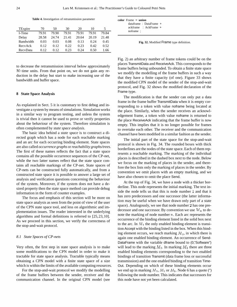
24 Lars M. Kristensen et al.: The Practitioner’s Guide to Coloured Petri Nets
Table 4. Investigation of retransmission parameter
TExpire 70 50 30 20 10 5I-Time 79.91 79.90 79.91 79.91 79.91 79.84Delay 28.58 24.74 21.41 20.64 20.19 21.48Bandwidth 0.03 0.03 0.08 0.13 0.24 0.45RecvAck 0.12 0.12 0.22 0.23 0.42 0.52RecvData 0.12 0.12 0.23 0.24 0.50 1.66
to decrease the retransmission interval below approximately30 time units. From that point on, we do not gain any re-duction in the delay but start to make increasing use of thebandwidth and buffer space.
8 State Space Analysis
As explained in Sect. 5 it is customary to first debug and in-vestigate a system by means of simulations. Simulation worksin a similar way to program testing, and unless the systemis trivial then it cannot be used to prove or verify propertiesabout the behaviour of the system. Therefore simulation isoften complemented by state space analysis.
The basic idea behind a state space is to construct a di-rected graph which has a node for each reachable markingand an arc for each occurring binding element. State spacesare also called occurrence graphs or reachability graphs/trees.The first of these names reflects the fact that a state spacecontains all the possible occurrence sequences of the CP-net,while the two latter names reflect that the state space con-tains all reachable markings of the CP-net. State spaces ofCP-nets can be constructed fully automatically, and from aconstructed state space it is possible to answer a large set ofanalysis and verification questions concerning the behaviourof the system. Moreover, if the system does not have a de-sired property then the state space method can provide debuginformation in the form of counter examples.
The focus and emphasis of this section will be more onstate space analysis as seen from the point of view of the userof the CPN state space tool, and less on algorithmic and im-plementation issues. The reader interested in the underlyingalgorithms and formal definitions is referred to [25,23,10].As we proceed in this section, we verify the correctness ofthe stop-and-wait protocol.
8.1 State Spaces of CP-nets
Very often, the first step in state space analysis is to makesome modifications to the CPN model in order to make ittractable for state space analysis. Tractable typically meansobtaining a CPN model with a finite state space of a sizewhich is within the limits of the available computing resources.
For the stop-and-wait protocol we modify the modellingof the frame buffers between the sender, receiver and thecommunication channel. In the original CPN model (see
color Frame = uniondataframe : DataFrame +ackframe : AckFrame +noframe ;
Fig. 32.Modified Frame type definition.
Fig. 2) an arbitrary number of frame tokens could be on theplaces TransmitData and ReceiveAck. This corresponds to theframe buffers being unbounded. To obtain a finite state spacewe modify the modelling of the frame buffers in such a waythat they have a finite capacity (of one). Figure 33 showsthe modified CPN model of the sender of the stop-and-waitprotocol, and Fig. 32 shows the modified declaration of theFrame type.
The modification is that the sender can only put a dataframe in the frame buffer TransmitData when it is empty cor-responding to a token with value noframe being located atthe place. Similarly, when the sender receives an acknowl-edgement frame, a token with value noframe is returned tothe place ReceiveAck indicating that the frame buffer is nowempty. This implies that it is no longer possible for framesto overtake each other. The receiver and the communicationchannel have been modified in a similar fashion as the sender.
The initial part of the state space for the stop-and-waitprotocol is shown in Fig. 34. The rounded boxes with thickborderlines are the nodes of the state space. Each of them rep-resents a reachable marking. The marking of the individualplaces is described in the dashed box next to the node. Belowwe focus on the marking of places in the sender, and there-fore the box lists only the marking of places in the sender. Byconvention we omit places with an empty marking, and wehave also chosen to omit the place Send.
At the top of Fig. 34, we have a node with a thicker bor-derline. This node represents the initial marking. The text in-side the node tells us that this is node number 1 and that ithas zero predecessors and one successor (the latter informa-tion may be useful when we have drawn only part of a statespace). Analogously, we see that node number 2 has one pre-decessor and one successor. By convention we use Mn to de-note the marking of node number n. Each arc represents theoccurrence of the binding element listed in the solid box nextto the arc. In M1 the only enabled binding element is transi-tion Accept with the binding listed in the box. When this bind-ing element occurs, we reach marking M2, in which there isagain one enabled binding element. An occurrence of Send-DataFrame with the variable dframe bound to (0,”Software”)will lead to the marking M3. In marking M3 there are threeenabled binding elements corresponding to the two enabledbindings of transition Transmit (data frame loss or successfultransmission) and the one enabled binding of transition Time-Out. Depending on which of these binding elements occurwe end up in marking M4, M5 or M6. Node 6 has a quote (”)following the node number. This indicates that successors forthis node have not yet been calculated.

Lars M. Kristensen et al.: The Practitioner’s Guide to Coloured Petri Nets 25
SendPacketBuffer
P I/O
Accept NextSend
SeqxStatus
ReceiveAckFrame
ReceiveAckFrame
noframe
I/OTransmitData
Frame
noframe
P I/O
SendDataFrame
Sending
DataFrame
TimeOut
Waiting
DataFrame
1‘(0,"")
ackframe rn
(sn,p)
dframe
dframe
p::packets
(sn,acked)
(sn,status)
if (rn > sn)then (rn,acked)else (sn, status)
(sn,notacked)
packets
dframe
dataframe dframe
dframe
dframe
(sn,notacked)
noframe
noframe
Fig. 33.Modified Sender of the stop-and-wait protocol.
From the first part of the state space it can be observedthat an occurrence of transition Transmit with the variablesuccess bound to false in M3 followed by the occurrence oftransition TimeOut leads via the marking M5 to the markingM2. An occurrence of the two binding elements in the op-posite order also leads from M3 to M2, but now with M4 asthe intermediate marking. The enabled binding of TimeOut isconcurrently enabled with each of the two bindings of transi-tion Transmit. By definition, arcs corresponding to steps withmore than one binding element are not part of the state space.Such arcs would give information about the concurrency be-tween binding elements, but they are not necessary for theverification of standard behavioural properties.
8.2 Generation of State Spaces
The CPN state space tool supports two modes in which theuser can generate state spaces: interactive and automatic. Therelationship between these two modes is similar to the rela-tionship between interactive and automatic simulations.
Interactive generation. In interactive generation the user spe-cifies a marking, and the tool then calculates the enabled bind-ing elements in this marking, and the successor marking re-sulting from the occurrence of each of these binding ele-ments. The first part of the state space for the stop-and-waitprotocol in Fig. 34 was obtained in this manner. Interactivegeneration is typically used in connection with drawing partsof the state space. We will return to this topic in Sect. 8.5.Interactive generation of the state space has many similaritieswith single step debugging.
Automatic generation. State spaces are in most cases of asize which makes it impractical to generate the full state space
in an interactive manner. Therefore it is also possible to gen-erate the state space in an automatic manner. Here the usersimply starts the generation and the state space is then calcu-lated by the state space tool fully automatically without anyintervention from the user. The user can control an automaticgeneration using so-called stop and branching options. Stopoptions allow the user to specify conditions under which thecalculation of the state space should be stopped. An exampleof this is to specify an upper bound on the number of nodesthat should be generated. The branching options give the userlocal control over the generation of successors, making it pos-sible to specify that only a certain subset of the successors ofa node should be generated. The generation control is partic-ularly important in early phases of state space analysis whichis typically concerned with identifying a configuration of thesystem which is tractable for state space analysis. The stopand branching options also make it possible to obtain a par-tial state space. A partial state space is a subset of the fullstate space. In many situations it is not necessary to gener-ate the full state space in order to locate errors and check thecorrectness of a system. A detailed discussion of partial statespaces is beyond the scope of this paper, and we will consideronly full state spaces in this section.
The state space of the stop-and-wait protocol has 1220
nodes, 3621 arcs and is generated in 4 seconds on a Sun UltraSparc with 300 Mb of memory. This is a rather small statespace and typically the state space consists of hundreds ofthousands of nodes and arcs. The CPN state space tool hasbeen used to construct state spaces with up to half a millionnodes and one million arcs (when the tool runs on a machinewith three hundred Megabytes of memory).

26 Lars M. Kristensen et al.: The Practitioner’s Guide to Coloured Petri Nets
1 0:1
1NextSend: 1‘(0,acked)Waiting: 1‘(0,"")ReceiveAck: 1‘noframeTransmitData: 1‘noframe
2 1:1
2 NextSend: 1‘(0,notacked)Sending: 1‘(0,"Software")ReceiveAck: 1‘noframeTransmitData: 1‘noframe
3 1:3
3NextSend: 1‘(0,notacked)Waiting: 1‘(0,"Software")ReceiveAck: 1‘noframeTransmitData: 1‘dataframe((0,"Software"))
4 1:2
4NextSend: 1‘(0,notacked)Sending: 1‘(0,"Software")ReceiveAck: 1‘noframeTransmitData: 1‘dataframe((0,"Software"))
5 1:1
5NextSend: 1‘(0,notacked)Waiting: 1‘(0,"Software")ReceiveAck: 1‘noframeTransmitData: 1‘noframe
6"1:0
1:1->2Accept: {sn=0, packets=[" Tools f","or Techn", "ology tr","ansfer. "], p="Software",dframe=(0,"")}
2:2->3SendDataFrame: {dframe=(0,"Software")}
3:3->4TimeOut: {sn=0, dframe=(0,"Software")}
4:3->5Transmit: {success=false,frame=dataframe((0,"Software"))}
5:3->6Transmit 1: {success=true,frame=dataframe((0,"Software"))}
8:4->2Transmit: {success=false,frame=dataframe((0,"Software"))}
10:5->2TimeOut: {sn=0, dframe=(0,"Software")}
Fig. 34.Initial part of the state space for the stop-and-wait protocol.
8.3 The State Space Report
When a state space has been generated, the next thing to dois typically to study the state space report. This is a text filecontaining answers to a set of standard behavioural propertieswhich can be used on any CPN model (i.e., generic proper-ties that can be formulated independently of the system underconsideration). The state space report can be produced in afew minutes – totally automatically. It contains a lot of highlyuseful information about the behaviour of the CPN model. Bystudying the state space report the user gets a first rough idea,as to whether the CPN model works as expected. If the sys-tem contains errors they are often reflected in the state spacereport. In the following we will go through the various partsof the state space report for the stop-and-wait protocol. Weonly give an intuitive explanation of the behavioural proper-ties. The reader interested in the formal definitions is referredto [22,25].
Statistical Information. The first part of the state space re-port contains some statistical information about the size ofthe state space. The statistical information for the state spaceof the stop-and-wait protocol is listed in Table 5. We see thatthe state space has 1220 nodes and 3621 arcs. We have cal-
culated the full state space, and this took only 4 seconds (ona Sun Ultra Sparc with 300 Mb of memory).
The statistical part also contains information about theSCC-graph [25]. A strongly connected component (SCC) isa maximal subgraph in which it is possible to find a path be-tween any pair of nodes, i.e., a part of the state space in whichall nodes are mutually reachable from each other. Each nodein the state space belongs to exactly one SCC and hence wecan use the SCCs to obtain a more compact graph known asthe SCC-graph. The SCC-graph has a node for each SCC andan arc for each binding element which leads from one SCCto another. Strongly connected components can be calculatedby Tarjan’s algorithm [18] which has a time and space com-plexity that is linear in the size of the state space. Hence, it ischeap to construct SCC-graphs and they turn out to be veryefficient for the investigation of certain kinds of behaviouralproperties [24,25]. From Table 5 we see that the SCC-graphhas 742 nodes and 2622 arcs. This means that there are lessSCCs (742) than state space nodes (1220), and hence at leastone of the SCCs covers more than one state space node. Fromthis we conclude that an infinite occurrence sequence exists,and hence we cannot be sure that the protocol terminates. Toguarantee termination one usually limits the number of re-transmissions.

Lars M. Kristensen et al.: The Practitioner’s Guide to Coloured Petri Nets 27
Table 5.Statistical Information.
State Space SCC GraphNodes: 1220 Nodes: 742Arcs: 3621 Arcs: 2622Secs: 4 Secs: 1Status: Full
Table 6.Upper and Lower Integer bounds.
Place Upper Bound Lower BoundNextSend 1 1ReceiveAck 1 1Send 1 1Sending 1 0TransmitData 1 1Waiting 1 0NextReceive 1 1ReceiveData 1 1Received 1 1TransmitAck 1 1
Boundedness Properties. The second part of the state spacereport contains information about the integer and multi-setbounds. Table 6 shows the upper and lower integer bounds,i.e., the maximal and minimal number of tokens which maybe located on the individual places in the reachable markings.The table only lists the places of the receiver and the sendersince the remaining places of the CP-net are related via portassignments to places either in the sender or in the receiver.This means that the integer bound for these places can beinferred from those in Table 6. From the table we see thateach of the places Sending and Waiting always has either oneor no token, while all other places always have exactly onetoken each. This is not at all surprising, but it is reassuring,since it indicates that the system behaves as expected.
Table 7 shows the upper multi-set bounds for the places inthe sender. By definition, the upper multi-set bound of a placeis the smallest multi-set which is larger than all reachablemarkings of the place. The integer bounds give us informa-tion about the number of tokens, while the multi-set boundsgive us information about the values which the tokens maycarry.
From the multi-set bounds we can, e.g., see that the placeTransmitData may contain all five different data frames and atoken with value noframe corresponding to the frame bufferbeing empty. We also see that no other token values are pos-sible for this place. Notice that the upper multi-set bound ofTransmitData is a multi-set with six elements, although theupper integer bound tells us that there can never be more thanone token on TransmitData at a time. Analogously, each ofthe places Sending and Waiting may contain all five possibledata frames. The place Waiting may in addition contain thedata frame (0,””) which is the data frame located on this placein the initial marking.
Also the upper multi-set bounds are as expected, and thisfurther confirms that the protocol works as expected. How-
Table 7.Upper Multi-set bounds.
NextSend 1‘(0,acked) + 1‘(0,notacked) +1‘(1,acked) + 1‘(1,notacked) +1‘(2,acked) + 1‘(2,notacked) +1‘(3,acked) + 1‘(3,notacked) +1‘(4,acked) + 1‘(4,notacked) +1‘(5,acked)
ReceiveAck 1‘ackframe(1) + 1‘ackframe(2) +1‘ackframe(3)+ 1‘ackframe(4) +1‘ackframe(5)+ 1‘noframe
Sending 1‘(0,”Software”) + 1‘(1,” Tools f”) +1‘(2,”or Techn”) + 1‘(3,”ology tr”) +1‘(4,”ansfer. ”)
TransmitData 1‘dataframe((0,”Software”)) +1‘dataframe((1,” Tools f”)) +1‘dataframe((2,”or Techn”)) +1‘dataframe((3,”ology tr”)) +1‘dataframe((4,”ansfer. ”)) +1‘noframe
Waiting 1‘(0,””) + 1‘(0,”Software”) +1‘(1,” Tools f”) + 1‘(2,”or Techn”) +1‘(3,”ology tr”) + 1‘(4,”ansfer. ”)
Send 1‘[”Software”,” Tools f”,”or Techn”,”ology tr”,”ansfer. ”] +
1‘[” Tools f”,”or Techn”,”ology tr”,”ansfer. ”] +
1‘[”or Techn”,”ology tr”,”ansfer. ”] +1‘[”ology tr”,”ansfer. ”] +1‘[”ansfer. ”] + 1‘[]
ever, the multi-set bounds also give us some new knowledge.As an example, there are probably many readers who did notnotice, until now, that acknowledgement frames never carrythe sequence number 0 as can be seen from the upper multi-set bound of the place ReceiveAck.
The lower multi-set bound of a place is the largest multi-set which is smaller than all reachable markings of the place.For all places in the stop-and-wait protocol the lower multi-set bound is the empty multi-set. This is because there are noplaces in the CPN model in which a token with a certain valueis permanently present.
Home and liveness properties. The third part of the statespace report is shown in Table 8. It provides information abouthome and liveness properties. A home marking is a markingwhich is reachable from all reachable markings, i.e., a mark-ing which can always be reached – independently of whathas previously happened. We see that the protocol has a sin-gle home marking, M862. A dead marking is a marking withno enabled transitions. We see that the protocol has a singledead marking, and that the dead marking is identical to the

28 Lars M. Kristensen et al.: The Practitioner’s Guide to Coloured Petri Nets
Table 8.Home and Liveness properties.
Home Markings: [862]Dead Markings: [862]Dead Transitions Instances: NoneLive Transitions Instances: None
8624:0
862Send: 1‘[]NextSend: 1‘(5,acked)Waiting: 1‘(4,"ansfer. ")ReceiveAck: 1‘noframeTransmitData: 1‘noframeReceiveData: 1‘noframeTransmitAck: 1‘noframeNextReceive: 1‘(5,acked)Received: 1‘["Software"," Tools f", "or Techn","ology tr", "ansfer. "]
Fig. 35.Home and dead marking.
home marking. At first glance, one might think that the exis-tence of dead markings would prevent the existence of homemarkings. However, by definition, a marking is always reach-able from itself, and hence a dead marking may be a homemarking (provided that it is the only dead marking). This isthe case for the protocol system. We will investigate the homeand dead marking in more detail in a moment.
From the liveness properties we also see that there are nodead transitions. Dead transitions are similar to dead code ina programming language and it means that each transition isenabled in at least one reachable marking (which is a ratherweak property). We also see that there are no live transitions.A live transition is a transition which can always, no matterwhat happens, become enabled again. When there are deadmarkings (as in our protocol), there cannot be any live transi-tions.
We now investigate marking M862 in more detail. Fig-ure 35 shows marking M862. Similarly to Fig. 34 the dashedbox next to the node gives information about the marking ofthe individual places. The box shows the marking of all placesin the sender and in the receiver with a non-empty marking.Inspection of the dashed box reveals that M862 is the desiredterminating state of the protocol, in which all data packetshave been sent, received in the correct order, and the framebuffers are empty. Since M862 is the only dead marking thisimplies that the protocol is partially correct – if the protocolterminates then it terminates in the desired state. Since M862
is a home marking the protocol always has a chance of ter-minating correctly. This means that it is impossible to reacha marking from which we cannot terminate the protocol withthe correct result.
Fairness Properties. The fourth and final part of the statespace report is shown in Table 9. It provides information aboutthe fairness properties, i.e., how often the individual transi-tions occur. We see that SendDataFrame, TimeOut, and Trans-
Table 9.Fairness properties.
Receive DataFrame FairSend AckFrame No FairnessAccept FairReceive AckFrame No FairnessSend DataFrame ImpartialTimeOut ImpartialTransmit 1 No FairnessTransmit 2 Impartial
mit 2 are impartial. This means that each of them occurs in-finitely often in any infinite occurrence sequence. Transmit 2is the transition on the second instance of page UniChannel.This is the instance which corresponds to the data channel.Hence, in any non-terminating execution of the protocol wekeep having timeouts and we keep sending and transmittingdata frames. Transition Accept is fair which is a weaker fair-ness property stating that the transition occurs infinitely oftenin all infinite occurrence sequences where it is infinitely oftenenabled.
8.4 Standard Queries
In addition to the state space report, the tool also offers aset of standard query functions that allow the user to make amore detailed inspection of the standard behavioural proper-ties. Many of these query functions return results which arealready included in the state space report as described in theprevious subsection. In fact, the state space report is imple-mented using a subset of the available standard query func-tions.
As an example, the tool has two functions, UpperInte-ger and LowerInteger which determine the maximal/minimalnumber of tokens residing on a set of places (where the statespace report only consider individual places). The queriesin Fig. 36 use these two functions to determine the max-imal/minimal number of tokens on the places Sending andWaiting.
It is easy to use the standard queries. For the queries inFig. 36, the only thing which the user has to do, is to declare afunction to be used as argument to UpperInteger and/or Low-erInteger. This function maps a marking Mn (of the entireCPN model) into the multi-set Mn(Sending)+Mn(Waiting).The result of both queries is 1, and hence we have proved thatthere always is a token on Sending or a token on Waiting, butnot on both places at the same time (see Fig. 33).
Analogously there is a function HomeSpace to determinewhether a specified set of markings constitute a home space,i.e., whether it always is possible to reach one of the specifiedmarkings - independently of what has previously happened.The argument to this function is a list containing the set ofmarkings under consideration.
The state space tool also provides standard queries to in-vestigate multi-set bounds and to investigate reachability. Fi-nally there are queries to investigate liveness and fairness

Lars M. Kristensen et al.: The Practitioner’s Guide to Coloured Petri Nets 29
fun SendWaitMarking n =(Mark.Sender'Sending 1 n) + (Mark.Sender'Waiting 1 n) ;
UpperInteger (SendWaitMarking) ;LowerInteger (SendWaitMarking) ;
Fig. 36.Example of standard query.
properties. These queries can be used on sets of transitionsor on sets of binding elements.
8.5 Visualisation of State Spaces
Since state spaces often become large, it seldom makes senseto draw them in full. However, the result of queries will oftenbe a set of nodes and/or arcs possessing certain interestingproperties, e.g., a path in the state space leading from onemarking to another. A good and quick way to get detailed in-formation on a small number of nodes and arcs is to draw thecorresponding fragment of the state space. This makes visu-alisation particularly useful when locating errors in a systemunder consideration.
The state space can be drawn either in small steps, e.g.,node by node or arc by arc, or in fragments using results from,e.g., queries as input to a number of built-in drawing func-tions. Drawing of state spaces is often done in conjunctionwith interactive generation. Figure 34 was obtained by com-bining interactive generation with drawing.
To obtain detailed information about the drawn fractionof the state space, it is possible to attach descriptors to thenodes and arcs. The boxes positioned next to the nodes andarcs in Fig. 34 are examples of descriptors. For the nodes, thedescriptors typically show the marking of certain places. Forthe arcs, the descriptors typically show the occurring transi-tion and the binding of some or all of its variables. The de-scriptors have sensible defaults but the user may customisethe descriptors by writing a script which specifies the con-tents and layout of the descriptor. The descriptors thus offeran abstraction mechanism by which the user can define a viewof the state space.
To illustrate the use of drawing in combination with de-bugging we investigate what will happen if we modify thestop-and-wait protocol such that we only send an acknowl-edgement frame back to the sender when we receive the dataframe that we were expecting. The state space for this vari-ant of the protocol has 261 nodes and 609 arcs. It has stillone dead marking in which all data packets have been sent,received in correct order, and the frame buffers are empty.However, this marking is no longer a home marking. This in-dicates that we can end up in a marking in which we cannotterminate the protocol correctly. To investigate this problem,we exploit the constructive feedback from the standard queryfunction for checking whether a marking is a home marking.This feedback tells us that there exists an SCC from whichit is impossible to reach the dead marking. By means of a
standard query function, we see that this SCC only has eightnodes and that one of these is node 15. Using another queryfunction we can find one of the shortest paths leading fromthe initial marking (node 1) to the node 15. This path is shownin Fig. 37, which is created by means of the built-in drawingfunctions. From the descriptors of the arcs on this path it iseasy to identify the problem. To begin with, we successfullytransmit the first data packet corresponding to the first threearcs in the path. Then we attempt to transmit the acknowl-edgement frame but it is lost. Hence, when we lose the ac-knowledgement frame we end up in a situation in which wecannot terminate the protocol correctly. The only thing thatcan happen from that point on is that we keep retransmittingthe first data frame. These retransmissions cannot trigger anacknowledgement frame which would allow us to start trans-mitting the next data frame. The latter can easily be seen bydrawing the eight nodes in the SCC together with the arcs thatinterconnect them.
8.6 Integration with Simulation
During a modelling and design process, the user quite oftenswitches between state space analysis and simulation. To sup-port this, the state space tool is tightly integrated with thesimulator, making it possible to transfer markings betweenthe simulator and the state space tool.
When a marking is transferred from the state space intothe simulator, it is displayed on the CPN diagram in the usualway. The user can inspect the marking of the individual places,and the enabling of the individual transitions. It is also pos-sible to start a simulation from the transferred marking. Asan example we could have checked that M862 was the de-sired dead marking by transferring the marking from the statespace tool into the simulator and inspect the marking of theindividual places. Figure 38 shows the top level page of thestop-and-wait protocol after M862 has been transferred intothe simulator.
Transferring the current marking of the simulator into thestate space is supported as well. A typical use of this is to in-vestigate all possible markings reachable within a few stepsfrom the current simulator marking. In this case, the usertransfers the simulator marking into the state space tool andall successor markings can be found and drawn as illustratedabove.
8.7 Advanced Queries
The state space report and the standard queries are good forproviding a rough picture of the behaviour of the system.However, they also have some limitations. First of all, manyinteresting properties of systems cannot easily be investigatedusing standard queries. Secondly, for debugging of systemsmore elaborated queries are often needed for locating thesource of the problem. Therefore a more general query lan-guage implemented on top of Standard ML (SML) is pro-vided. It provides primitives for traversing the state space in

30 Lars M. Kristensen et al.: The Practitioner’s Guide to Coloured Petri Nets
1 0:1
2 3:1
3 1:3
6 1:2
8 3:2
113:3
153:1
1:1->2Accept: {sn=0, packets= [" Tools f","or Techn", "ology tr","ansfer. "], p="Software", dframe=(0,"")}
2:2->3SendDataFrame : {dframe=(0,"Software")} 5:3->6
Transmit: {success=true,frame=dataframe((0,"Software"))}
9:6->8Receive: {status=acked, sn=0,rn=0,packets=[], p="Software"}
13:8->11SendAckFrame : {rn=1}
20:11->15Transmit: {success=false,frame=ackframe(1)}
Fig. 37.Occurrence sequence as debugging information.
Send
PacketBuffer
1 1‘[]
Sender
Communication Channel
Receiver
Received
PacketBuffer
1 1‘["Software"," Tools f","or Techn","ology tr","ansfer. "]
TransmitData
Frame
1 1‘noframe
ReceiveAck
Frame
1 1‘noframe
TransmitAck
Frame
1 1‘noframe
ReceiveData
Frame
1 1‘noframe
Fig. 38.Home and dead marking of the protocol.
different ways and thereby writing non-standard and modeldependent queries. On top of this general query language, avariant of the temporal logic CTL is provided [5]. In this vari-ant of CTL, it is possible to formulate queries about bindingelements as well as markings corresponding to Petri nets be-ing both action and state oriented.
Similar to standard queries, a non-standard query typi-cally consists of a few lines of SML code. To illustrate thiswe will use the query language to investigate a system de-pendent property of the stop-and-wait protocol. We want tocheck that the sender is at most one data packet ahead of thereceiver, i.e., that the stop-and-wait discipline is observed bythe protocol. This can be proved by the non-standard querylisted in Fig. 39. SWPredicate is a predicate which, given amarking, checks that the sum of the lengths of the lists onthe places Send and Received differs by at most one fromthe total number of data packets to be sent. PredAllNodes isa predeclared query function, which returns all the nodes inthe state space that satisfy a specified predicate. In the querywe negate the SWPredicate and hence check the state space
val Length = length o ms to col ;val total = Length (Mark.Sender'Send 1 1)
fun SWPredicate n =let
val sent = total � (Length (Mark.Sender'Send 1 n)) ;val received = (Length (Mark.Receiver'Receiver 1 n))
in((sent = received) orelse (sent = received + 1))
end ;
val nodelist = PredAllNodes (not o SWPredicate) ;
Fig. 39.Example of non-standard query.
for nodes which violates the predicate. The operator o is thebuilt-in infix operator in SML for functional composition.
For the state space of the stop-and-wait protocol the resultof the query is the empty list. Hence all nodes in the statespace satisfy the SWPredicate, and we have proved that thestop-and-wait discipline is observed.
8.8 Advanced State Space Analysis
In this section, we have demonstrated that the state spacemethod is an effective way to investigate the dynamic be-haviour of a system. The construction and analysis of statespaces are totally automatic. From the state space report theuser gains a lot of knowledge about the dynamic behaviour ofthe system. The state space method, however, also has somedrawbacks.
The most serious drawback of the state space method isthe so-called state explosion problem. For many systems, thestate space becomes so large that it cannot be fully constructedeven for small configurations of the system. A number oftechniques exist for alleviating the state explosion problem.

Lars M. Kristensen et al.: The Practitioner’s Guide to Coloured Petri Nets 31
They do this by constructing a condensed state space fromwhich it is still possible to verify the same kind of behaviouralproperties as with full ordinary state spaces. Condensed statespaces are typically orders of magnitude smaller than the fullstate space. Some of the techniques exploit the symmetry [25,23,30] and equivalence [25,29] which are present in manyconcurrent and distributed systems. Other techniques exploitthe independency and concurrency between binding elements[31], or take advantage of the hierarchical structure of theCPN model [12]. The reader is encouraged to consult thepapers cited above for a more detailed presentation and dis-cussion of these techniques, their use, and how they are sup-ported by the CPN state space tool.
Another drawback is the fact that a state space is alwaysconstructed for a particular initial marking, which often cor-responds to only one out of many different possible systemconfigurations. Above we have seen that the protocol workswhen we have five data packets – but will it also work formore packets? In theory we cannot be totally sure. However,in practice the situation is not that bad, since most errors insystem designs tend to manifest themselves already in smallconfigurations. Hence, it is very likely that our protocol alsowill work with more than five packets.
9 Conclusions
Coloured Petri Nets have been developed over the past 20years at the University of Aarhus, Denmark. The develop-ment has been balanced between the development of theory,supporting computer tools, and experiments in the form ofpractical case studies. All three parts have had a mutual ben-eficial influence on each other. The development of theory hasbeen driven by the idea of combining the concurrency theoryof Petri nets with the practical applicability of high-level pro-gramming languages. The theory has been important for de-veloping computer tools founded on a solid and sound theory.The development of computer tools has been necessary to beable to make practical experiments with the aim of assessingthe practical applicability of the developed theory. The prac-tical case studies have led to new theoretical developments.A number of the case studies have been conducted by ex-ternal users. This has provided valuable input for the furtherdevelopment of CP-nets and their supporting tools, and hasdemonstrated the practical applicability of CP-nets.
In this paper we have demonstrated the application ofCP-nets for modelling and analysis of a rather simple com-munication protocol. It is obvious that compared to a simplecommunication protocol considerably more effort has to beinvested when modelling and analysing industrial-sized sys-tems. The feasibility of doing this has been demonstrated in alarge number of different projects. This includes the projectsdescribed in the subsequent papers of this special section onColoured Petri Nets. Other examples are projects within theareas of communication protocols [16,21], audio/ video sys-tems [8], operating systems [6,7], hardware designs [17,45],embedded systems [43], software system designs [33,44], and
business process re-engineering [35,40] and the industrialprojects listed on the web site [37]. The reader is referred tothe individual papers for an elaborated assessment of the re-sources needed to apply CP-nets on industrial-sized systems.
As part of larger case studies (see e.g., [8,43]) knowledgehas also been gained on the resources, which people with-out prior knowledge of CP-nets, need to invest in order tobe able to start applying CP-nets. The experiences have beenencouraging. Typically, only about one or two weeks of inten-sive training are needed in order to be able to construct andsimulate the first CPN models. CP-nets and the Design/CPNtool have been used in a course on distributed systems [11] atthe University of Aarhus. After a period of about four weeks(with 15 hours of work per week) the students are able tomake a CPN model of a non-trivial protocol stack and vali-date its correctness by means of simulations.
A comprehensive web site has been set up [37] with re-sources and technical support on the use of CP-nets and theDesign/CPN tool. It contains manuals, tutorials, examples,answers to frequently asked questions (FAQs), list of knownproblems, tips and tricks etc. Moreover, it explains how to geta free license for the Design/CPN tool. The tool is currentlyavailable for Sun Solaris, HP Unix and Linux platforms. Amailing list has been established as a forum for discussionamong users of the Design/CPN tool.
The first workshop on practical use and application of CP-nets and Design/CPN (CPN’98) [28] was held in Aarhus inJune, 1998 with the participation of 40 users from 10 differ-ent countries. The workshop contained presentations of regu-lar papers, tutorials with practical exercises, and discussionsand presentations of future plans for Design/CPN. Selectedpapers from the workshop are published in this special sec-tion of the STTT journal. The second workshop CPN’99 willbe held in Aarhus in October, 1999.
The first version of Design/CPN appeared in 1989. Basedon the knowledge gained from the practical use of the tool,the internal data structures and algorithms of the CPN simu-lator have been re-designed and are currently in the process ofbeing implemented. The first results show that the new simu-lator runs orders of magnitude faster than the current versionof the CPN simulator. The new simulator also contains animproved interface for declarations of types, variables, andfunctions. This new interface reduces the turn-around timebetween the editor and simulator when working with large-scale CPN models. The first version of this new simulator isreleased in 1999. A similar development is planned for theCPN state space tool. This work is expected to significantlypush the borderline of systems that can be analysed by statespaces.
The area of automatic code generation from CP-nets isalso a topic of ongoing work. Until now CP-nets have mostlybeen applied for design and analysis of systems, and the tran-sition to the final implementation has been done manually.Some first experiments in the area of automatic code genera-tion were reported in [43]. The promising work of this projectis currently being continued.

32 Lars M. Kristensen et al.: The Practitioner’s Guide to Coloured Petri Nets
Acknowledgements. Many students and colleagues – in particularat University of Aarhus and Meta Software – have influenced thedevelopment of CP-nets, their analysis methods and their tool sup-port. The development has been supported by several grants fromthe Danish Natural Science Research Council. A more detailed de-scription of individual contributions can be found in the prefaces of[24–26]. For the present paper, we are grateful for the comments andsuggestions provided by the reviewers.
References
1. A.W. Appel and D.B. MacQueen. Standard ML of New Jersey.In J. Maluszynski and M. Wirsing, editors, Third InternationalSymposium on Programming Languages Implementation andLogic Programming, volume 528 of Lecture Notes in ComputerScience. Springer-Verlag, 1991.
2. D. Bertsekas and R Gallager. Data Networks. Prentice-Hall,1992.
3. C. Capellmann, S. Christensen, and U. Herzog. Visualising theBehaviour of Intelligent Networks. In T. Margaria, B. Steffen,R. Ruckert, and J. Posegga, editors, Services and Visualisation,Towards User-Friendly Design, volume 1385 of Lecture Notesin Computer Science, pages 174–189. Springer-Verlag, 1998.
4. ITU (CCITT). Recommendation z.120: Msc. Technical report,International Telecommunication Union, 1992.
5. A. Cheng, S. Christensen, and K.H. Mortensen. Model Check-ing Coloured Petri Nets Exploiting Strongly Connected Com-ponents. In M.P. Spathopoulos, R. Smedinga, and P. Kozak, ed-itors, Proceedings of WODES’96. Institution of Electrical Engi-neers, Computing and Control Division, Edinburgh, UK, 1996.
6. L. Cherkasova, V. Kotov, and T. Rokicki. On Net Modellingof Industrial Size Concurrent Systems. In M. Ajmone-Marsan,editor, Proceedings ICATPN’93, volume 691 of Lecture Notesin Computer Science. Springer-Verlag, 1993.
7. L. Cherkasova, V. Kotov, and T. Rokicki. On Scalable Net Mod-eling of OLTP. In Proceedings of the 5th International Work-shop on Petri Nets and Performance Models, Toulouse, France.IEEE Computer Society Press, 1993.
8. S. Christensen and J.B. Jørgensen. Analysis of Bang andOlufsen’s BeoLink Audio/Video System Using Coloured PetriNets. In P. Azema and G. Balbo, editors, ProceedingsICATPN’97, volume 1248 of Lecture Notes in Computer Sci-ence. Springer-Verlag, 1997.
9. S. Christensen, J.B. Jørgensen, and L.M. Kristensen. De-sign/CPN - A Computer Tool for Coloured Petri Nets. InE. Brinksma, editor, Proceedings of TACAS’97, volume 1217 ofLecture Notes in Computer Science, pages 209–223. Springer-Verlag, 1997.
10. S. Christensen and L.M. Kristensen. State Space Analysis ofHierarchical Coloured Petri Nets. In B. Farwer, D. Moldt, andM-O. Stehr, editors, Proceedings of Workshop on Petri Nets inSystem Engineering – Modelling, Verification, and Validation,pages 32–43. Department of Computer Science, University ofHamburg, 1997. Report no. 205.
11. S. Christensen and K.H. Mortensen. Teaching Coloured PetriNets - A Gentle Introduction to Formal Methods in a Dis-tributed Systems Course. In P. Azema and G. Balbo, editors,Proceedings of ICATPN’97, volume 1248 of Lecture Notes inComputer Science, pages 290–309. Springer-Verlag, 1997.
12. S. Christensen and L. Petrucci. Modular State Space Analysisof Coloured Petri Nets. In G. De Michelis and M. Diaz, editors,
Proceedings of ICATPN’96, volume 935 of Lecture Notes inComputer Science. Springer-Verlag, 1996.
13. Meta Software Corp. http://www.metasoftware.com.14. Meta Software Corporation. Design/OA. Meta Software Cor-
poration, 150 Cambridge Park Drive, Cambridge MA 02140,USA.
15. J. Billington et al. High-level Petri Nets – Concepts, Def-initions and Graphical Notation. Technical report, Interna-tional Standards Organization and International Electrotechni-cal Committee, October 1997. Commitee Draft 15909 ISO/IECJTC1/SC7/WG11 N-3.
16. D.J. Floreani, J. Billington, and A. Dadej. Designing and Ver-ifying a Communications Gateway Using Coloured Petri Netsand Design/CPN. In J. Billington and W. Reisig, editors, Pro-ceedings of ICATPN’96, volume 1091 of Lecture Notes in Com-puter Science. Springer-Verlag, 1996.
17. H.J. Genrich and R.M. Shapiro. Formal Verification of an Ar-biter Cascade. In K. Jensen, editor, Proceedings ICATPN’92,volume 616 of Lecture Notes in Computer Science. Springer-Verlag, 1992.
18. A. Gibbons. Algorithmic Graph Theory. Cambridge UniversityPress, 1985.
19. C. F. Goldfarb and Y. Rubinsky. The SGML handbook. Claren-don Press, Oxford, UK, 1990.
20. The CPN Group. http://www.daimi.au.dk/CPnets.21. P. Huber and V.O. Pinci. A Formal Executable Specification of
the ISDN Basic Rate Interface. In G. Rozenberg, editor, Pro-ceedings ICATPN’91, 1991.
22. K. Jensen. An Introduction to the Theoretical Aspects ofColoured Petri Nets. In J.W. de Bakker, W.-P. de Roever,and G. Rozenberg, editors, A Decade of Concurrency, volume803 of Lecture Notes in Computer Science, pages 230–272.Springer-Verlag, 1994.
23. K. Jensen. Condensed State Spaces for Colored Petri Nets. For-mal Methods of System Design, 9, 1996.
24. K. Jensen. Coloured Petri Nets. Basic Concepts, Analysis Meth-ods and Practical Use. Volume 1, Basic Concepts. Mono-graphs in Theoretical Computer Science. Springer-Verlag,1997. ISBN: 3-540-60943-1.
25. K. Jensen. Coloured Petri Nets. Basic Concepts, Analy-sis Methods and Practical Use. Volume 2, Analysis Meth-ods. Monographs in Theoretical Computer Science. Springer-Verlag, 1997. ISBN: 3-540-58276-2.
26. K. Jensen. Coloured Petri Nets. Basic Concepts, Analysis Meth-ods and Practical Use. Volume 3, Practical Use. Monographs inTheoretical Computer Science. Springer-Verlag, 1997. ISBN:3-540-62867-3.
27. K. Jensen. An Introduction to the Practical Use of ColouredPetri Nets. In W. Reisig and G. Rozenberg, editors, Lectureson Petri Nets II, volume 1492 of Lecture Notes in ComputerScience, pages 237–292. Springer Verlag, 1998.
28. K. Jensen, editor. Workshop on Practical Use of Coloured PetriNets and Design/CPN, number 532 in DAIMI PB. Departmentof Computer Science, University of Aarhus, 1998. Also avail-able via http://www.daimi.au.dk/CPnets/workshop98/papers/.
29. J. B. Jørgensen and L.M. Kristensen. Verification of ColouredPetri Nets Using State Spaces with Equivalence Classes. InB. Farwer, D. Moldt, and M-O. Stehr, editors, Proceedings ofWorkshop on Petri Nets in System Engineering – Modelling,Verification, and Validation, pages 20–31. Department of Com-puter Science, University of Hamburg, 1997. Report no. 205.
30. J.B. Jørgensen and L.M. Kristensen. Computer Aided Verifi-cation of Lamport’s Fast Mutual Exclusion Algorithm Using

Lars M. Kristensen et al.: The Practitioner’s Guide to Coloured Petri Nets 33
Coloured Petri Nets and Occurrence Graphs with Symmetries.To Appear in IEEE Transactions on Parallel and DistributedSystems, 1999.
31. L. M. Kristensen and A. Valmari. Finding Stubborn Setsof Coloured Petri Nets Without Unfolding. In J. Desel andM. Silva, editors, Proceedings of ICATPN’98, volume 1420 ofLecture Notes in Computer Science, pages 104–123. Springer-Verlag, 1998.
32. R.B. Lyngsø and T. Mailund. Textual Interchange Formatfor High-level Petri Nets. In K. Jensen, editor, Workshop onPractical Use of Coloured Petri Nets and Design/CPN, num-ber 532 in DAIMI PB, pages 47–65. Department of Com-puter Science, University of Aarhus, 1998. Also available viahttp://www.daimi.au.dk/CPnets/workshop98/papers/.
33. W.M. McLendon and R.F. Vidale. Analysis of an Ada Sys-tem Using Coloured Petri Nets and Occurrence Graphs. InK. Jensen, editor, Proceedings ICATPN’92, volume 616 of Lec-ture Notes in Computer Science. Springer-Verlag, 1992.
34. R. Milner, R. Harper, and M. Tofte. The Definition of StandardML. MIT Press, 1990.
35. K.H. Mortensen and V. Pinci. Modelling the Work Flow ofa Nuclear Waste Management Program. In R. Valette, edi-tor, Proceedings of ICATPN’94, volume 815. Springer-Verlag,1994.
36. T. Murata. Petri Nets: Properties, Analysis and Application.In Proceedings of the IEEE, Vol. 77, No. 4. IEEE ComputerSociety, 1989.
37. Design/CPN Online. http://www.daimi.au.dk/designCPN/.38. The Gnuplot Tool. Available online: http://www.cs.dartmouth/
gnuplot info.html.39. L. C. Paulson. ML for the Working Programmer. Cambridge
University Press, 2 edition, 1996.40. V.O. Pinci and R.M. Shapiro. An Integrated Software Develop-
ment Methodology Based on Hierarchical Coloured Petri Nets.In G. Rozenberg, editor, Advances in Petri Nets, volume 524 ofLecture Notes in Computer Science, pages 227–252. Springer-Verlag, 1991.
41. Information Processing:. Text and office systems: StandardGeneralized Markup Language (sgml). Technical report, ISOstandard 8879, International Organisation for Standardization,Geneve, Switzerland, 1986. Amendment from 1988 exists.
42. J. L. Rasmussen and M. Singh. Mimic/CPN. A Graphical Sim-ulation Utility for Design/CPN. User’s Manual.
43. J.L. Rasmussen and M. Singh. Designing a Security System byMeans of Coloured Petri Nets. In J. Billington and W. Reisig,editors, Proceedings of ICATPN’96, volume 1091 of LectureNotes in Computer Science. Springer-Verlag, 1996.
44. G. Scheschonk and M. Timpe. Simulation and Analysis of aDocument Storage System. In R. Valette, editor, Proceedings ofICATPN’94, volume 815 of Lecture Notes in Computer Science.Springer-Verlag, 1994.
45. R.M. Shapiro. Validation of a VLSI Chip Using HierarchicalColoured Petri Nets. Journal of Microelectronics and Reliabil-ity, Special Issue on Petri Nets, 1991.
46. J.D. Ullman. Elements of ML Programming. Prentice-Hall,1997.
47. L. Wells and B. Lindstrøm. The Design/CPN PerformanceTool Manual. Department of Computer Science, University ofAarhus, 1998.