a coloured petri net approach for spatial biomodel ...ceur-ws.org/vol-1373/paper3.pdf · a coloured...

A coloured Petri net approach for spatialBiomodel Engineering based on the modularmodel composition framework Biomodelkit

Mary Ann Blätke1ú and Christian Rohr2ú

1 Otto-von-Guericke University Magdeburg,Chair of Regulatory Biology

Universitätsplatz 2, D-39106 Magdeburg, [email protected]

http://www.regulationsbiologie.de/

2 Brandenburg University of Technology Cottbus-Senftenberg,Chair of Data Structures and Software Dependability,

Postbox 10 13 44, D-03013 Cottbus, Germany,[email protected],

http://www-dssz.informatik.tu-cottbus.de

Abstract. Systems and synthetic biology require multiscale biomodelengineering approaches to integrate diverse spatial and temporal scalesin order to understand and describe the various interactions in biologicalsystems. Our BioModelKit framework for modular biomodel engineeringallows to compose multiscale models from a set of modules, each describ-ing an individual molecular component in the form of a Petri net. In thisframework, we do now propose a feature for spatial modelling of molec-ular biosystems. Our spatial modelling methodology allows to representthe local positioning and movement of individual molecular componentsrepresented as modules. In the spatial model, interactions between com-ponents are restricted by their local positions. In this context, we usecoloured Petri nets to scale the modular composed spatial model, suchthat each molecular component can exist in an arbitrary number of in-stances. Thus, a modular composed spatial model can be mapped to thecellular arrangement and di�erent cell geometries.

Keywords: Modular Model Composition, Spatial Modelling, MultiscaleBiomodel Engineering, Coloured Petri nets

1 Introduction

Systems biology aims at describing and understanding complex biological pro-cesses on a systems level. Therefore, systems biology employs modelling andsimulation as indispensable tools to describe, predict and understand biologicalsystems in an integrative and quantitative context. Besides complex interactions,

ú Corresponding authors

M Heiner, AK Wagler (Eds.): BioPPN 2015, a satellite event of PETRI NETS 2015, CEUR Workshop Proceedings Vol. 1373, 2015.

38 MA Blätke, C Rohr

models do also need to integrate diverse temporal and spatial scales spanningthe biological systems. Multiscale biomodel engineering goes beyond standardmodelling approaches in systems biology and addresses physical problems as im-portant features at multiple scales in time and space [1]. Current challenges andmethodologies used so far in multiscale biomodel engineering have been reviewedin [2] and [3].

Here, we focus on the spatial aspects in multiscale biomodel engineering,which have been mostly neglected in the description of intracellular processesuntil now [1]. In particular, we demonstrate, based on the BioModelKit frame-work for modular biomodel engineering [4], how to extend plain models of intra-cellular processes to spatial models without their reimplementation. The modelsin our case are composed from modules, where each module describes the func-tionality of a certain molecular component in the form of a Petri net. The useof coloured Petri nets in our approach allows to represent di�erent numbers ofmodule instances for each component. To our knowledge, the methodology forspatial modelling in the context of modular model composition, which we suggestin this paper, is unique.

As modelling tool, we chose Snoopy [5], because it supports low-level andcoloured Petri net network classes, as well as the concept of logical (fusion)nodes and hierarchical modelling.

In the next section, we will shortly describe the BioModelKit framework andsummarize the use of coloured Petri nets for multiscale modelling. Afterwards,in Section 3, we introduce our spatial modelling methodology as a new featureof the BioModelKit framework. Section 4 applies the introduced methodologyfor spatial modelling to a simple example of a molecular interaction between twoproteins represented as modules. In the last section, we give a short summaryand outlook.

2 Previous Work

2.1 BioModelKit Framework for Modular Model Composition

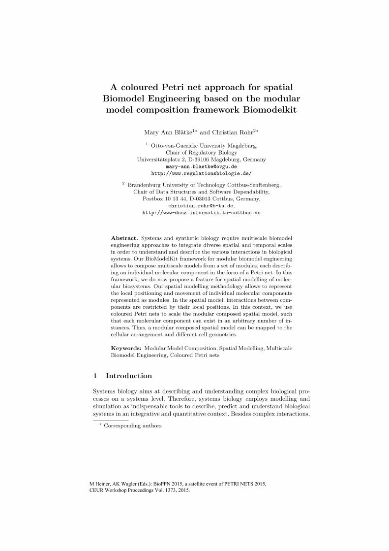
The BioModelKit framework (BMK framework) is a tool for modular biomodelengineering [4], see Fig. 1. The main motivation behind BMK framework wasto develop a modelling environment, where modules are specifically designed forthe purpose of model composition. The modularisation approach used in BMKframework was inspired by the natural composition of biomolecular systems,where molecular components (genes, mRNAs and proteins) are the main build-ing blocks. Thus, each molecular component is represented as a self-containedmodule, describing the underlying functionality using the formal language ofPetri nets. Interface networks, which are part of each module describe the inter-actions with other molecular components and are used to automatically couplerespective modules [4].

Since, the functionality of genes, mRNAs and proteins is diverse, di�erentmodule types have been defined in BMK framework, as well as allelic influence

Proc. BioPPN 2015, a satellite event of PETRI NETS 2015

Spatial modelling based on modular modelling 39

Modules

Biomodelkit Database

Set of Modules

Spatial Models

Wildtype/

Alternative

Models

Model-based Predictions

GeneModules

mRNAModules

ProteinModules

ProteinDegrdation

Modules

Causal InfluenceModules

AllelicInfluenceModules

Biomolecular Systems

Experimental Data

Boolean Networks

Molecular Mechanisms

SBML Models

<sbml>...

</sbml>

Forward Engineering

ReverseEngineering

Transformation Transformation

UploadModel Composition

High-Throughput Analysis

Add Modules to Collection

+ Algorithmic Mutation

+ Space-Attributes

Fig. 1: Overview of the BioModelKit Framework for Modular Model Composi-tion.

modules and causal influence modules to capture also correlations with missingmechanistic descriptions [6,7]. Modules can be generated by forward and reverseengineering approaches or by transforming boolean models or models providedin the systems biology markup language (SBML) into modules [8,9], see Fig. 1.

The web-interface of BMK framework (www.biomodelkit.com [4]) includes afeature to submit modules and to create a model annotation file in the BMKmarkup language (BMKml, unpublished work). The submitted module and itsannotation have to be curated by an administrator before publicly releasing themby storing their content in a relational MySQL database (BMKdb). Anotherfeature of the BMK framework is a model composition algorithm, which allowsto automatically compose comprehensive models from a set of chosen modules.In addition, the composed model can also be modified by applying algorithmsmimicking single/double gene knock-outs or structural mutations of the includedmolecular components (unpublished work).



2.2 Coloured Petri Nets

We use Petri nets (PN ) as modelling paradigm, which gives us a completeformalised and standardised framework, as well as an intuitive way of modellingconcurrent behaviour.

In systems biology, as well as in other fields, it’s quite common that parts oflarger models have similar structures. In such a case simplifying the model viareusing that part, instead of having redundant structures is demanded. ColouredPetri nets (PN C) are a modelling paradigm that fits well in such a case.

We are using Snoopy [10] as modelling and simulation tool, thus we describePN C how they are defined there.

coloursets:

enum species := red, green, blue

product complex := species, species

variables:

species x

species y

species

2‘green++

1‘blueB

complex

AB

species

2‘red++

1‘green

A

[x<>y]

x

y

(x,y)

(a) Before Firing

species

2‘green

B

complex

1‘(green,blue)

AB

species

2‘red

A

[x<>y]

x

y

(x,y)

(b) After Firing

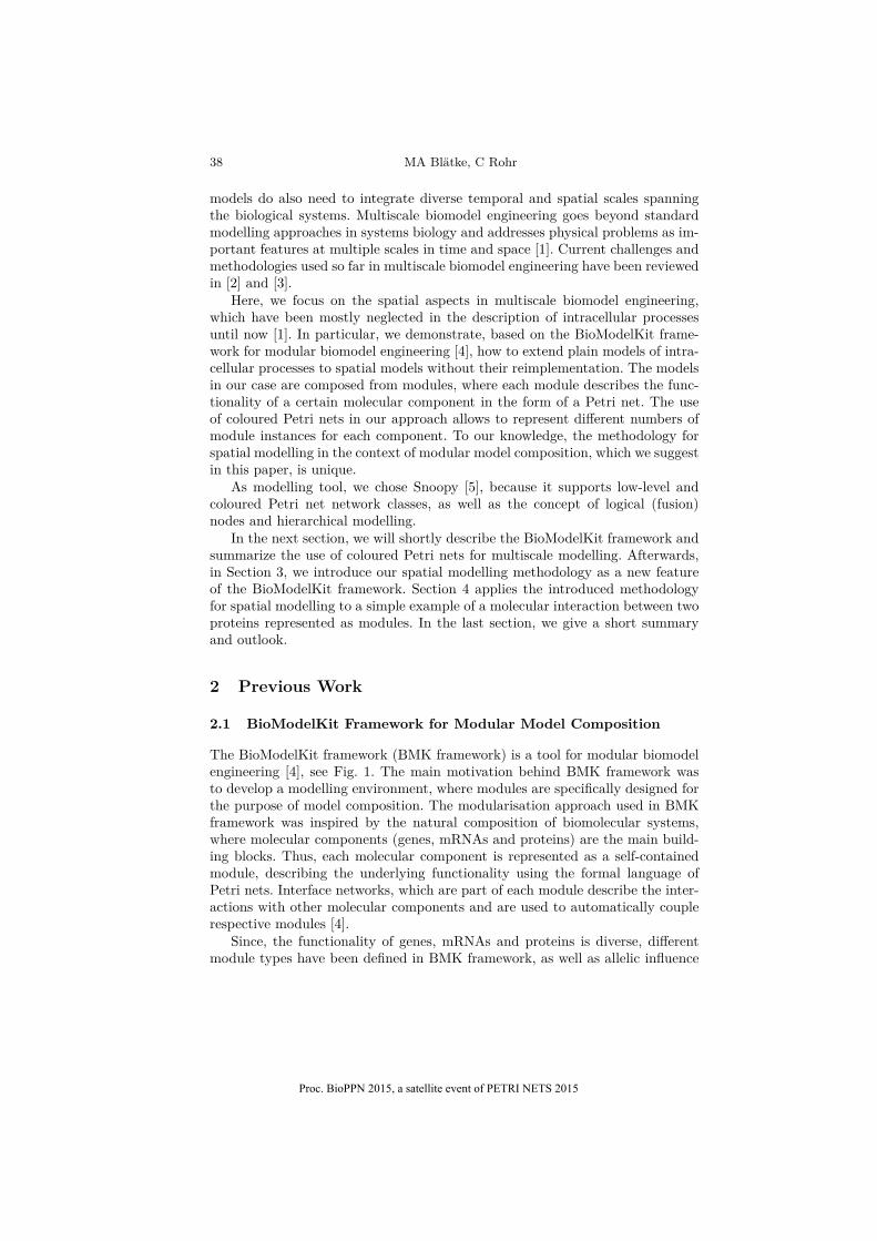
Fig. 2: Example PN C of abstract complex formation.

We use the coloured Petri net in Fig. 2 as an example. It represents an ab-stract complex formation of two species of di�erent kind into one complex. Themodel contains two coloursets, first a simple colourset named species of typeenum, including the colours red, green and blue. Second a product coloursetnamed complex, its colours are 2-tuples of the species colourset. The net consistsof three places A, B and AB and one transition. The colourset species is asso-ciated with the places A and B and the place AB has colourset complex. Thevariables x and y are used in the arc inscriptions and the transition guard. Thetransition guard x <> y determines that only tokens of di�erent colour are validbindings for the variables x and y. The arc inscriptions x and y on the incoming

We summarize the following net classes together under the term Petri net (PN ):Qualitative Petri net (QPN ), eXtended Petri net (X PN ), Continuous Petri net(CPN ), Stochastic Petri net (SPN ) and Hybrid Petri net (HPN ). The same goesfor the coloured Petri nets (PN C).



arcs of the transition define its precondition, i.e. there have to be at least onetoken on place A and one token on place B and they have to be of di�erentcolour due to the guard. The arc inscription (x, y) on the outgoing arc of thetransition defines the production of one complex token. In Fig. 2a the place A

has two tokens of colour red and one token of colour green and the place B hastwo tokens of colour green and one token of colour blue. This gives the followingbindings for the variables x and y: (red, green), (red, blue), (green, blue). We se-lected the binding (green, blue) and let the transition fire. One green token fromplace A and one blue token from place B are consumed and one (green, blue)token is produced on place AB, see Fig. 2b.

Much more extensive descriptions how to use coloured Petri nets in systemsbiology are given in [11,12,13]. Besides the animation of the coloured Petri net,it is possible to unfold every PN C into an uncoloured PN [11]. So it is possibleto apply any analysis and simulation technique available for uncoloured Petrinets on coloured Petri nets too.

Up to this, modelling biochemical systems using coloured Petri nets did notincorporate spatial aspects or movement in space. But this can be included inthe model as shown by Gilbert et al. [14]. Therefore the space is discretised intoa grid of one, two or three dimensions and a position in the grid is representedby a single place. This works fine if there is no need to distinguish between theentities on each position. One can model the di�usion of substances using thisapproach quite well, as presented in [14].

This can be extended to more complex reaction-di�usion systems, as shownin [15]. More examples of using coloured Petri nets for modelling of biologicalsystems including spatial aspects are [16,17].

All models above have in common that they model space by discretisationinto a grid and having one subnet (ranging from a single place to a complexnetwork) per grid position. This is handy, if the entities moving around have nointernal behaviour or state and there is no need to distinguish them. But if thatis the case, the internal network has to move around as well and this leads tosome issues on modelling and simulation. Parvu et al. [17] used this approachfor a model of phase variation in bacterial colony growth. The bacteria havetwo di�erent states, i.e. two places A and B representing the two states andtwo transitions for changing the state are needed. In order to let the bacteriamove around, the whole subnet is needed in every grid position. Incorporatingthis in the coloured model is straightforward, but the size of the unfolded modelincreases drastically. This has an impact on the analysis and simulation of themodel and may lead to inconvenient run times.

While the approaches of representing space via discretisation into grid-placesfit well in the shown cases, it is not practical in our use case, because we havecomplex subnets moving around. We present our approach of incorporating spaceby adding coordinate places in the following section.



3 Spatial Modelling Methodology for Modular ComposedModels

Before we start with the formal description of the spatial transformation al-gorithm, we have to introduce some general definitions which apply to ourmodular modelling approach. A module Mi is defined by a quintuple Mi =(Pi, Ti, fi, vi, m

0,i) according to the general definition of quantitative Petri nets.Each module Mi consists of nci + 1 components, the main component C

0

andnci interacting components. Thus, each module Mi represents a set of compo-nents Ci = {C

0

, C1

, . . . , Cnci}. The mapping of a place pij œ Pi of a module

Mi to a set of components C

pij

i ™ Ci is given by the relation g : Pi æ Ci,such that g(pi

j) = C

pij

i . A place pij with |g(pi

j)| > 1 represents a complex

of |g(pij)| components. The set Ki = {C

pij

i | |g(pij)| > 1} contains all com-

plexes among the components in Ci. A transition tij œ Ti of a module Mi with

|g(•tij)flg(ti

j•)| > 1 represents an interaction with at least two di�erent involvedcomponents. The total set of all interacting transitions in a Module Mi is givenby T IA

i = {’tij œ Ti : |g(•ti

j) fl g(tij•)| > 1}.

A set of modules defines a modular composed model M = {M1

, . . . , Mn},where n is the number of modules. Consequently, the modular composed modelcan also be defined as M = (P M, T M, fM, vM, mM

0

) according to the generaldefinition of quantitative Petri nets with the following relations:

– P M =t

Pi, where Mi œ M - total finite and non-empty set of places.– T M =

tTi, where Mi œ M - total finite and non-empty set of transitions.

– fM =t

fi, where Mi œ M - total set of directed arcs, weighted by a non-negative integer value.

– vM :t

Ti æ H, where Mi œ M - total set of firing rates.– mM

0

tPi æ N

0

, ÷pikÕ , pj

kÕÕ with pikÕ œ Pi, pj

kÕÕ œ Pj , wherepi

kÕ = pjkÕÕ , {pi

kÕ : pjkÕÕ} æ pM

k œ P M, mM0

(pMk ) = max(m

0,i(pikÕ), m

0,j(pjkÕÕ))

In addition to the definitions above, the following relations can be derived:

– C

M =t

Ci , where Mi œ M - total set of components– gM :

tPi æ

tCi, where Mi œ M - total set of place component relations

– T MIA ™ T M =

tT IA

i , where Mi œ M - total set of all interacting transitions– KM =

tKi, where Mi œ M - total set of complexes.

Spatial Transformation Algorithm For the spatial transformation of theflat modular composed model the following procedure needs to be executed.

Step 1: Explicit Encoding of Local Positions. The position of each componentCi œ CM is explicitly encoded by d places pCi

1

, . . . pCid (termed coordinate places),

which can be interpreted as coordinates, where d, d Ø 1, defines the number ofaxes (e.g. 1D, 2D or 3D grid). The marking m(pCi

j ) of a place pCij defines the

current coordinate value, which must be restricted by a lower mL(pCij ) and



upper bound mU (pCij ) to represent the boundaries of the encoded grid, such

that, mL/U (pCij ) > 0 and mL(pCi

j ) < mU (pCij ).

Step 2: Local Restriction of Interactions. To restrict the executability of eachtransition t œ T M

IA , the firing rate h(t) must be multiplied by a boolean relationb(t) describing a defined neighbourhood relation: hIA(t) = b(t) ú h(t), t œ T M

IA .If the neighbourhood relation claims that the distance between components in-volved in the interaction represented by a transition t œ T M

IA must be zero, b(t)has to be defined as follows:

b(t) =I

1,q|g(•t)fig(t•)|≠1

i=1

q|g(•tfig(t•)|j=i+1

qdk=1

(m(pCik ) ≠ m(pCj

k ))2 = 00,

q|g(•t)fig(t•)|≠1

i=1

q|g(•t)fig(t•)|j=i+1

qdk=1

(m(pCik ) ≠ m(pCj

k ))2 ”= 0In addition, read edges, connecting each transition t œ T M

IA and the coordinateplaces of the respective components have to be added, such thatfReadEdge(pg(•t)fig(t•)

1≠d , t) = 1.

Step 3: Explicit Encoding of Local Position Changes. To encode the positionchanges for a component Ci œ CM two di�erent scenarios have to be considereddependent on the state of interaction:1. Local position change of individual components:

For each component Ci œ C

M and each coordinate place pCij œ {pCi

1

, . . . , pCid }

two transitions tCij,L and tCi

j,U are needed to incrementally decrease or increasethe amount of tokens. The transition tCi

j,L subtracts tokens from the coordi-nate place pCi

j till m(pCij ) = mL(pCi

j ). Therefore, the following edges haveto be introduced fM(pCi

j , tCij,L) = 1 and fM

ReadEdge(pCij , tCi

j,L) = mL(pCij ) + 1.

The transition tCij,U adds tokens to the coordinate place pCi

j till m(pCij ) =

mU (pCij ). Therefore, the following edges have to be introduced

fM(tCij,U , pCi

j ) = 1 and fMInhibitorEdge(pCi

j , tCij,U ) = mU (pCi

j ). To ensure thatthe position of the component Ci can only be changed if it does not in-teract with another component Cj , i ”= j, additional inhibitory edges foreach transition tCi

j,L/U have to be introduced: fInhibitorEdge(P CiIS , tCi

j,L/U ) = 1,where P Ci

IS ™ P M and P CiIS = {’p œ P M : Ci œ g(p) · |g(p)| > 1}.

2. Local position change of complexes:The local position of components forming a complex ki œ KM have to beupdated consistently during the local position change. For each complexki œ KM and each dimension j, 1 Æ j Æ d, two transitions tki

j,L and tkij,U are

needed to incrementally decrease or increase the amount of tokens. The tran-sition tki

j,L removes tokens from the set of coordinate placest

ChœkipCh

j till atleast for one component Ch œ C

M the condition m(pChj ) = mL(pCh

j ) is ful-filled. Therefore, for each component Ch œ ki the following edges have to beintroduced fM(pCh

j , tkij,L) = 1 and fM

ReadEdge(pChj , tki

j,L) = mL(pChj ) + 1. The

transition tkij,U adds tokens to the set of coordinate places

tChœki

pChj till at

least for one component Ch œ C

M the condition m(pChj ) = mU (pCh

j ) is ful-filled. Therefore, for each component Ch œ ki the following edges have to be



introduced fM(tkij,U , pCh

j ) = 1 and fMInhibitorEdge(pCh

j , tkij,U ) = mU (pCh

j ). Toensure that the position of the complex ki can only be changed if it is actuallyformed additional read edges for each transition tki

j,L/U have to be introduced:fReadEdge(P ki

IS , tki

j,L/U ) = 1, where P kiIS ™ P M and

P kiIS = {’p œ P M | ki = g(p)}. Furthermore, it must be excluded for each

component Ch œ ki that interacts with other components using a di�erentbinding site. Therefore, all co-existing interactions have to be determinedKki

coex = {’kj œ KM : ki fl kj ”= ? | kj ”= ki}. All places representing acomplex kj œ Kki

coex have to be added to each transition tki

j,L/U using aninhibitory edge: fInhibitoryEdge(P ki

COEX , tki

j,L/U ) = 1, where P kiCOEX = {’p œ

P M : g(p) = k, k œ Kkicoex}.

To allow the movement of co-existing complexes which use di�erent interac-tion sites simultaneously, the above described procedure has to be appliedto all possible combination of co-existing complexes, compare Section 4.

For simplicity reasons the firing rate of each transition tki

j,L/U and tCh

j,L/U

is given by Fick’s laws of di�usion [18]. Furthermore, we assume equidistantsubvolumes with the width and hight h = 1 and set all di�usion coe�cient toone. Please note, it is straightforward to define the di�usion coe�cients moreprecisely based on experimental results.

Step 4: Encoding of Component Instances by Applying Coloured Petri nets. Acolourset ‡simple

Ciwith 1 ≠ qCi colours needs to be specified for each component

Ci œ C

M, where qCi œ N defines the number of instances for a component Ci.The total set of simple coloursets is given by Àsimple = {‡simple

C1, . . . , ‡simple

|CM| }.For each ‡simple

Ciœ Àsimple a variable aCi needs to be specified. All edges f(p, t)

and f(t, p) of the flat model M for which it is true, that a component Ci œC

M, where Ci œ g(p) and |g(p)| = 1 are extended to the multiset expressionaCi ‘f(p, t), or respectively aCi ‘f(t, p). The total set of simple coloursets Àsimple

is mapped to a subset of places according to the relation Ssimple : Àsimple æP M, such that Ssimple(‡simple

Ci) = {p œ P M | Ci œ g(p) · |g(p)| = 1}.

Each complex ki œ KM, where ki represents a subset of components, suchthat ki ™ CM, is represented by a compound colourset of type product‡compound

ki=

rCjœki

‡simpleCj

. The total set of compound coloursets is given byÀcompound = {‡compound

k1, . . . , ‡compound

|KM| }. The total set of compound coloursetsÀcompound is mapped to remaining subset of places according to the relationScompound : Àcompound æ P M, such thatScompound(‡compound

ki) = {p œ P M | ki = g(p)}. All edges f(p, t) and f(t, p) of

the flat model M for which its is true, that a complex ki œ KM, where ki = g(p)are extended to the multiset expression

tCjœki

aCj ‘f(p, t), or respectivelyt

CjœkiaCj ‘f(p, t). The marking and firing rates are kept constant over all place

and transition instances, such that marking of each place p œ P M is represented



by all()‘m0

(p) and the firing rates of each transition t œ T M all()‘h(t), whereall() is a function that extracts all instances of a coloured node.

4 Example

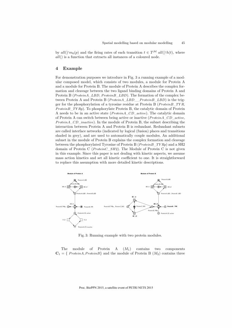
For demonstration purposes we introduce in Fig. 3 a running example of a mod-ular composed model, which consists of two modules, a module for Protein Aand a module for Protein B. The module of Protein A describes the complex for-mation and cleavage between the two ligand binding domains of Protein A andProtein B (P roteinA_LBD, P roteinB_LBD). The formation of the complex be-tween Protein A and Protein B (P roteinA_LBD__P roteinB_LBD) is the trig-ger for the phosphorylation of a tyrosine residue at Protein B (P roteinB_T Y R,P roteinB_T Y Rp). To phosphorylate Protein B, the catalytic domain of ProteinA needs to be in an active state (P roteinA_CD_active). The catalytic domainof Protein A can switch between being active or inactive (P roteinA_CD_active,P roteinA_CD_inactive). In the module of Protein B, the subnet describing theinteraction between Protein A and Protein B is redundant. Redundant subnetsare called interface networks (indicated by logical (fusion) places and transitionsshaded in grey), and are used to automatically couple modules. An additionalsubnet in the module of Protein B explains the complex formation and cleavagebetween the phosphorylated Tyrosine of Protein B (P roteinB_T Y Rp) and a SH2domain of Protein C (P roteinC_SH2). The Module of Protein C is not givenin this example. Since this paper is not dealing with kinetic aspects, we assumemass action kinetics and set all kinetic coe�cient to one. It is straightforwardto replace this assumption with more detailed kinetic descriptions.

Module of Protein BModule of Protein A

ProteinA LBD ProteinA LBD

ProteinB LBD ProteinB LBD

ProteinA LBD ProteinB LBD ProteinA LBD ProteinB LBD

ProteinA CD active ProteinA CD active

ProteinB TYRp

ProteinB TYRp

ProteinA CD inactive

ProteinB TYRp ProteinC SH2 ProteinC SH2ProteinB TYR ProteinB TYR

AB t3 AB t3

AB t1 AB t1AB t2 AB t2

A t2 A t1

BC t2

BC t1

Fig. 3: Running example with two protein modules.

The module of Protein A (M1

) contains two componentsC

1

= { P roteinA, P roteinB} and the module of Protein B (M2

) contains three



components C

2

= {P roteinA, P roteinB, P roteinC}. For the composed ModelM = {M

1

, M2

}, we get the following mapping of places to the components:

– gM({P roteinA_LBD, P roteinA_CD_active, P roteinA_CD_inactive})=P roteinA

– gM({P roteinB_LBD, P roteinB_T Y R, P roteinB_T Y Rp}) =P roteinB

– gM({P roteinB_SH2}) =P roteinC

– gM({P roteinA_LBD__P roteinB_LBD}) = {P roteinA, P roteinB}– gM({P roteinB_T Y Rp__P roteinC_SH2}) = {P roteinB, P roteinC}

Furthermore places P roteinA_LBD__P roteinB_LBD andP roteinB_T Y Rp__P roteinC_SH2 represent two complexesk

1

= {P roteinA, P roteinB} and k2

= {P roteinB, P roteinC}. The set of inter-acting transitions is given by T M

IA = {AB_r1, AB_r2, AB_r3, BC_r1, BC_r2}.For the spatial model we assume a two dimensional grid (d = 2) of the size

5◊5 for each component given by the constants xDimA = xDimB = xDimC = 5and yDimA = yDimB = yDimC = 5.

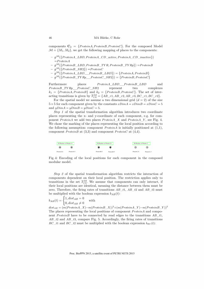
Step 1 of the spatial transformation algorithm introduces two coordinateplaces representing the x- and y-coordinate of each component, e.g. for com-ponent P roteinA we add two places P roteinA_X and P roteinA_Y , see Fig. 4.We chose the marking of the places representing the local position according tothe following assumption: component P roteinA is initially positioned at (1,1),component P roteinB at (3,3) and component P roteinC at (4,4).

XY-Position of Protein CXY-Position of Protein BXY-Position of Protein A

ProteinB YProteinA YProteinA X ProteinB X

4

ProteinC X

4

ProteinC Y

Fig. 4: Encoding of the local positions for each component in the composedmodular model.

Step 2 of the spatial transformation algorithm restricts the interaction ofcomponents dependent on their local position. The restriction applies only totransitions in the set T M

IA . We assume that components can only interact, iftheir local positions are identical, meaning the distance between them must bezero. Therefore, the firing rates of transitions AB_t1, AB_t2 and AB_t3 mustbe multiplied with the boolean expression bAB(t):

bAB(t) =I

1, distAB = 00, distAB ”= 0

with

distAB = (m(P roteinA_X)≠m(P roteinB_X))2+(m(P roteinA_Y )≠m(P roteinB_Y ))2

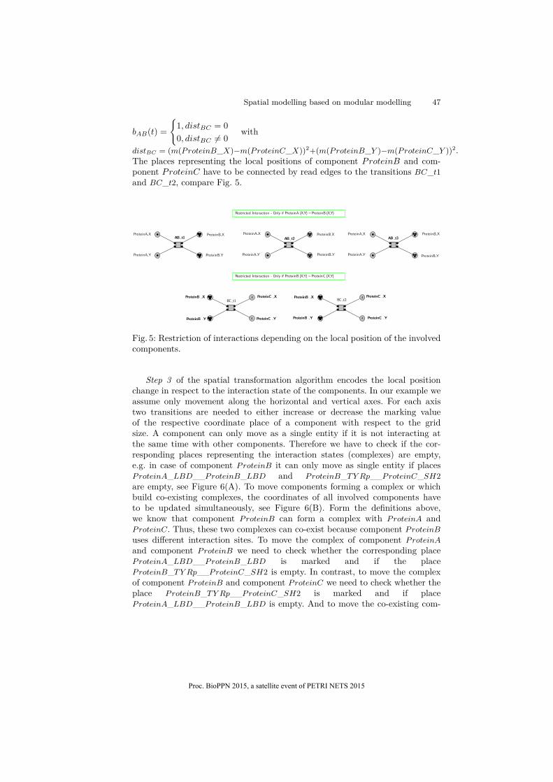
The places representing the local positions of component P roteinA and compo-nent P roteinB have to be connected by read edges to the transitions AB_t1,AB_t2 and AB_t3, compare Fig. 5. Accordingly, the firing rates of transitionsBC_t1 and BC_t2 must be multiplied with the boolean expression bBC(t):



bAB(t) =I

1, distBC = 00, distBC ”= 0

with

distBC = (m(P roteinB_X)≠m(P roteinC_X))2+(m(P roteinB_Y )≠m(P roteinC_Y ))2.The places representing the local positions of component ProteinB and com-ponent ProteinC have to be connected by read edges to the transitions BC_t1and BC_t2, compare Fig. 5.

Restricted Interaction - Only if ProteinB (X,Y) =ProteinC (X,Y)

Restricted Interaction - Only if ProteinA (X,Y) =ProteinB (X,Y)

ProteinB Y

ProteinB Y

ProteinB Y ProteinB Y ProteinB YProteinA Y ProteinA Y ProteinA Y

ProteinA X ProteinA X ProteinA X

ProteinB X

ProteinB X

ProteinB X ProteinB X ProteinB X

ProteinC X

ProteinC X

ProteinC Y

ProteinC Y

AB t3

AB t1

AB t2

BC t2BC t14

4

4

4

Fig. 5: Restriction of interactions depending on the local position of the involvedcomponents.

Step 3 of the spatial transformation algorithm encodes the local positionchange in respect to the interaction state of the components. In our example weassume only movement along the horizontal and vertical axes. For each axistwo transitions are needed to either increase or decrease the marking valueof the respective coordinate place of a component with respect to the gridsize. A component can only move as a single entity if it is not interacting atthe same time with other components. Therefore we have to check if the cor-responding places representing the interaction states (complexes) are empty,e.g. in case of component P roteinB it can only move as single entity if placesP roteinA_LBD__P roteinB_LBD and P roteinB_T Y Rp__P roteinC_SH2are empty, see Figure 6(A). To move components forming a complex or whichbuild co-existing complexes, the coordinates of all involved components haveto be updated simultaneously, see Figure 6(B). Form the definitions above,we know that component P roteinB can form a complex with P roteinA andP roteinC. Thus, these two complexes can co-exist because component P roteinB

uses di�erent interaction sites. To move the complex of component P roteinA

and component P roteinB we need to check whether the corresponding placeP roteinA_LBD__P roteinB_LBD is marked and if the placeP roteinB_T Y Rp__P roteinC_SH2 is empty. In contrast, to move the complexof component P roteinB and component P roteinC we need to check whether theplace P roteinB_T Y Rp__P roteinC_SH2 is marked and if placeP roteinA_LBD__P roteinB_LBD is empty. And to move the co-existing com-



plex of component P roteinA, component P roteinB and component P roteinC, weneed to check if both places P roteinA_LBD__P roteinB_LBD andP roteinB_T Y Rp__P roteinC_SH2 are marked.

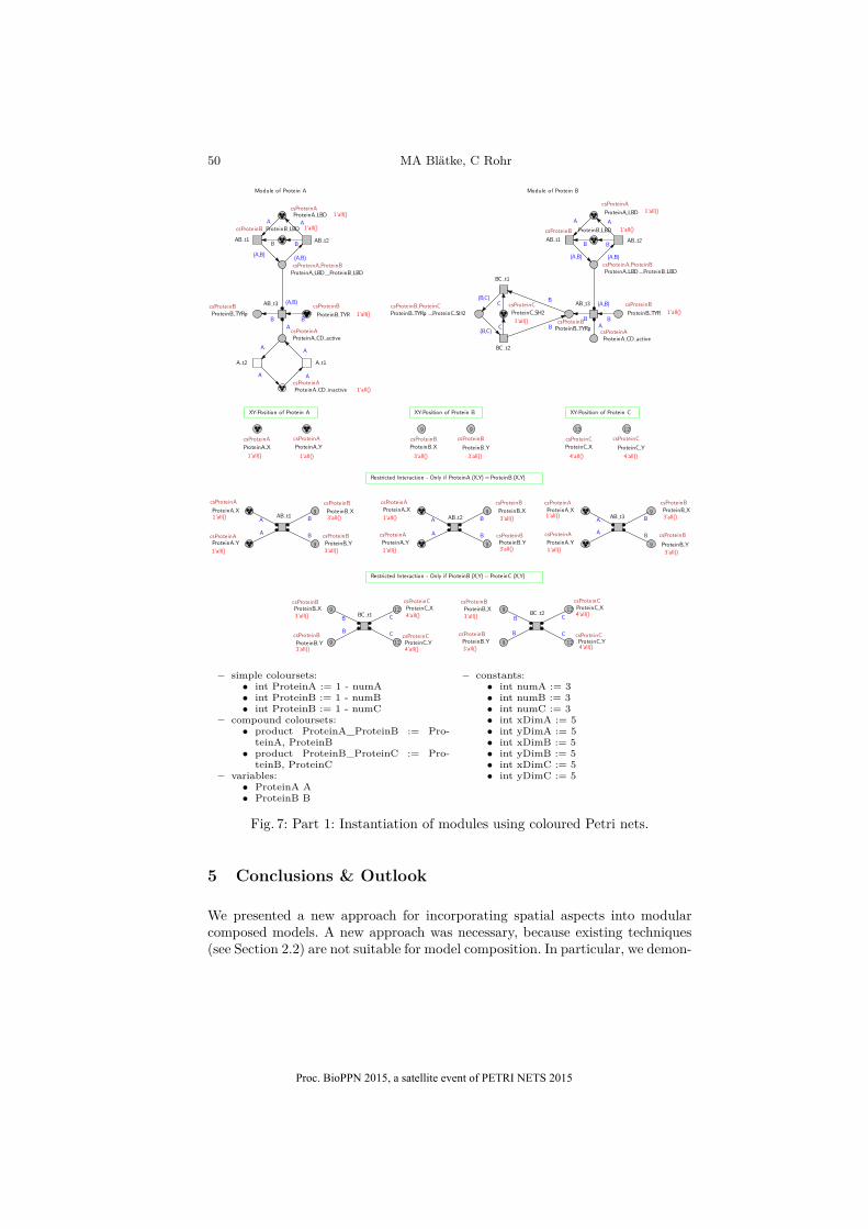
Step 4 of the spatial transformation algorithm has to be applied to representmore than one instance of each component, compare Fig. 7 and 8. In our examplethe number of instances for each component is three, which we represent by theconstants numA = numB = numC = 3. For each component Ci œ C

M we definea simple colourset:

– int csProteinA := 1 - numA,– int csProteinB := 1 - numB,– int csProteinC := 1 - numC

where colourset csP roteinA is mapped to the places with the relationg(p) =P roteinA, colourset csP roteinB is mapped to the places with the rela-tion g(p) =P roteinB and colourset csP roteinC is mapped to the places whichfulfil relation g(p) =P roteinC. The coordinate places of each component have tobe bound to the respective colourset as well. Furthermore, we need to define avariable for each simple colourset:

– csProteinA A– csProteinB B– csProteinC C

All in-going and out-going arcs of places bound to one of the simple coloursets de-fined above have to carry the respective variable as arc expression. Since, we havetwo binary complexes k

1

= {P roteinA, P roteinB} and k2

= {P roteinB, P roteinC},we need to define a compound colourset for each as product of the respectivesimple coloursets:

– product csProteinA_ProteinB := csProteinA, csProteinB– product csProteinB_ProteinC := csProteinB, csProteinC

where colourset csP roteinA_P roteinB is mapped to the places with the relationg(p) = {P roteinA, P roteinB} and colourset csP roteinB_P roteinC is mapped tothe places with the relation g(p) = {P roteinB, P roteinC}. All in-going and out-going arcs of places bound to one of the compound coloursets defined above haveto carry a 2-tuple of respective variables as arc expression.

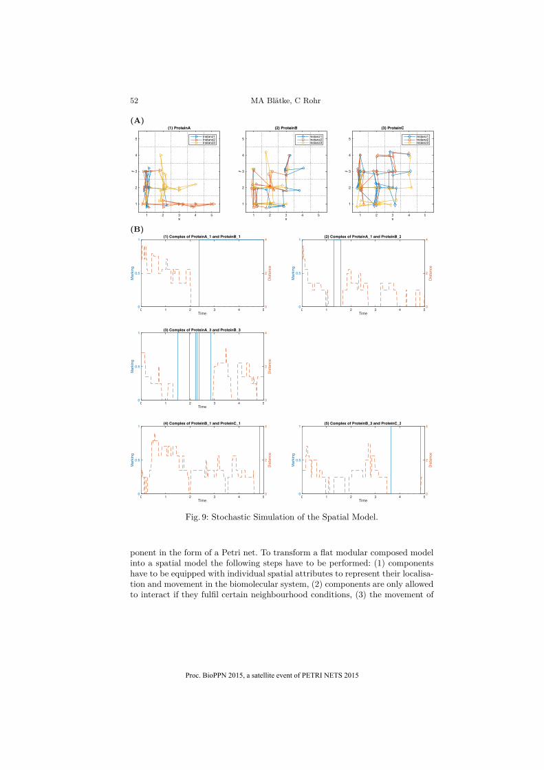
Fig. 9 presents one exemplifying stochastic simulation run of the final spatialmodel of Fig. 7 and 8. In Fig. 9(A), we depict the movement of all instances ofcomponents P roteinA, P roteinB and P roteinC on separate two-dimensional gridsof the size 5◊5. During the simulation time three complexes between instances ofcomponent P roteinA and component P roteinB could be obtained (P roteinA_1+P roteinB_1,P roteinA_1+P roteinB_2,P roteinA_3+P roteinB_3), as well as twocomplexes between instances of component P roteinB and component P roteinC

(P roteinB_1 + P roteinC_1,P roteinB_3 + P roteinC_3). The simulation resultalso shows that the distance between the corresponding instances of compo-nents forming a complex is zero, which means that they can only move has oneentity. Subfigure (1) and (2) of Fig. 9(B) shows that the instance P roteinB1 isinteracting with instance P roteinA1 and instance P roteinC1 at the same timenear the end of the simulation run, thus the two complex states co-exist.



(A)

Movement of Protein CMovement of Protein BMovement of Protein A

ProteinA LBD ProteinB LBD




ProteinB Y

ProteinB TYRp ProteinC SH2




ProteinA Y

ProteinA X ProteinB XProteinC X

ProteinC Y

XL A XR A

YU AYD A YL B YD B

XR BXL B

YD A YU A

XR AXL A

2

2

2

2 2

2xDimA

yDimA

xDimB

yDimB yDimC

xDimC

4

4

(B)

Movement of complex ProteinA ProteinB ProteinCMovement of complex ProteinB ProteinCMovement of complex ProteinA ProteinB





ProteinB Y ProteinB Y ProteinB Y


ProteinB TYRp ProteinC SH2 ProteinB TYRp ProteinC SH2

ProteinB TYRp ProteinC SH2 ProteinB TYRp ProteinC SH2


ProteinA Y

ProteinA Y

ProteinA X

ProteinA X

ProteinB X ProteinB X ProteinB X

ProteinC X ProteinC X

ProteinC Y ProteinC Y

YL AB YD AB

XR ABXL AB XL BC XR BC

YU BCYD BC YD ABC YU ABC

XR ABCXL ABC

2

2

2

2 2

2

2

2 2

2

2

2

yDimA

xDimA

yDimB

xDimB xDimB

yDimB

xDimC

yDimC yDimC

xDimC

yDimB

xDimB

xDimA

yDimA

4 4

4 4

Fig. 6: Local position change dependent on the state of interaction. (A) compo-nents are not in complex, (B) components are in complex with each other.



Restricted Interaction - Only if ProteinB (X,Y) =ProteinC (X,Y)

XY-Position of Protein C

Restricted Interaction - Only if ProteinA (X,Y) =ProteinB (X,Y)

XY-Position of Protein BXY-Position of Protein A

Module of Protein BModule of Protein A

csProteinA1‘all()ProteinA LBD

csProteinA1‘all()ProteinA LBD

csProteinB 1‘all()ProteinB LBD csProteinB 1‘all()ProteinB LBD

csProteinA ProteinBProteinA LBD ProteinB LBD


csProteinAProteinA CD active

csProteinAProteinA CD active

csProteinBProteinB TYRp

csProteinBProteinB TYRp

csProteinBcsProteinB

csProteinB

3‘all()3‘all()

3‘all()9

ProteinB YProteinB Y

ProteinB Y

csProteinB

3‘all()

9

ProteinB Y

csProteinB

3‘all()9 ProteinB Y

csProteinB

3‘all()9 ProteinB Y

csProteinA1‘all()ProteinA CD inactive

csProteinB ProteinCProteinB TYRp ProteinC SH2

csProteinC

1‘all()

ProteinC SH2

csProteinA

1‘all()

ProteinA Y

csProteinA

1‘all()

ProteinA Y

csProteinA

1‘all()ProteinA Y

csProteinA

1‘all()ProteinA Y

csProteinA

1‘all()

ProteinA X

csProteinA

1‘all()ProteinA X

csProteinA

1‘all()

ProteinA XcsProteinA

1‘all()ProteinA X

csProteinBcsProteinB

csProteinB

3‘all()3‘all()

3‘all()9

ProteinB XProteinB X

ProteinB X

csProteinB

3‘all()

9

ProteinB X

csProteinB

3‘all()9 ProteinB X

csProteinB

3‘all()9 ProteinB X

csProteinB csProteinB1‘all()1‘all()ProteinB TYR ProteinB TYR

csProteinCcsProteinC

csProteinC

4‘all()4‘all()

4‘all()

12

ProteinC XProteinC X

ProteinC X

csProteinC csProteinC

csProteinC

4‘all() 4‘all()

4‘all()

12

ProteinC Y ProteinC Y

ProteinC Y

AB t3 AB t3

AB t3AB t1

AB t1 AB t1

AB t2

AB t2 AB t2

A t2 A t1

BC t2

BC t2BC t1

BC t1

AA

B B

(A,B)

(A,B)

(A,B)(A,B)

A A

B

B

B

B

AA

AA

(B,C)C

B

BC(B,C)

B B

(A,B)

(A,B)

A A

A

A

A

A

A

AB

B

B

B

B

B

CC BB

BB CC

9

9

9

9

12

12

12

12

– simple coloursets:

• int ProteinA := 1 - numA

• int ProteinB := 1 - numB

• int ProteinB := 1 - numC

– compound coloursets:

• product ProteinA_ProteinB := Pro-

teinA, ProteinB

• product ProteinB_ProteinC := Pro-

teinB, ProteinC

– variables:

• ProteinA A

• ProteinB B

– constants:

• int numA := 3

• int numB := 3

• int numC := 3

• int xDimA := 5

• int yDimA := 5

• int xDimB := 5

• int yDimB := 5

• int xDimC := 5

• int yDimC := 5

Fig. 7: Part 1: Instantiation of modules using coloured Petri nets.

5 Conclusions & Outlook

We presented a new approach for incorporating spatial aspects into modularcomposed models. A new approach was necessary, because existing techniques(see Section 2.2) are not suitable for model composition. In particular, we demon-



Movement of complex ProteinAProteinB ProteinCMovement of complex ProteinBProteinC

Movement of Protein CMovement of Protein BMovement of Protein A

Movement of complex ProteinAProteinB


csProteinA ProteinB


csProteinA ProteinB




csProteinA ProteinB






csProteinB

3‘all()

9

ProteinB Y

csProteinB

3‘all()9

ProteinB YcsProteinB

3‘all()9

ProteinB YcsProteinB

3‘all()9

ProteinB Y


csProteinB ProteinC


csProteinB ProteinC


csProteinB ProteinC








csProteinA

1‘all()

ProteinA Y

csProteinA

1‘all()

ProteinA Y

csProteinA

1‘all()

ProteinA Y

csProteinA

1‘all()

ProteinA X

csProteinA

1‘all()

ProteinA X

csProteinA

1‘all()

ProteinA X

csProteinB

3‘all()9

ProteinB X

csProteinB

3‘all()

9

ProteinB XcsProteinB

3‘all()

9

ProteinB XcsProteinB

3‘all()

9

ProteinB X

csProteinC

4‘all()

ProteinC X

csProteinC

4‘all()

12

ProteinC XcsProteinC

4‘all()

12

ProteinC X

csProteinC

4‘all()

ProteinC Y

csProteinC

4‘all()12

ProteinC YcsProteinC

4‘all()12

ProteinC Y

XL A XR A

YU AYD A YD B YU B

XR BXL B

YD AB YU AB

XR ABXL AB

YD C YU C

XR CXL C

XL BC XR BC

YU BCYD BC YD ABC YU ABC

XR ABCXL ABC

A A

AA

B B

B B

A A

AA

B B

B B

C C

CC

BB

BB

C C

CC C C

CC

B B

B BA

A

A A

2‘A

2‘A

2‘B

2‘B

2‘A

2‘A

(A,B)(A,B)

(A,B) (A,B)

2‘B

2‘B

2‘C

2‘C

2‘B

2‘B

2‘C

2‘C

(B,C) (B,C)

(B,C) (B,C) (B,C)(B,C)

(B,C)(B,C)

2‘C

2‘C

2‘B

2‘B

(A,B) (A,B)

(A,B) (A,B)

2‘A

2‘A

xDimA‘A

yDimA‘A

xDimB‘B

yDimB‘B

yDimA‘A

xDimA‘A

yDimB‘B

xDimB‘B

(A,all()) (A,all())

(A,all()) (A,all())

(all(),B) (all(),B)

(all(),B) (all(),B)

(B,all()) (B,all())

(B,all()) (B,all())

(all(),C)(all(),C)

(all(),C)(all(),C)

yDimC‘C

xDimC‘C

(B,all()) (B,all())

(B,all()) (B,all())

xDimB‘B

yDimB‘B

xDimC‘C

yDimC‘C

(all(),B) (all(),B)

(all(),B) (all(),B)

yDimC‘C

xDimC‘C

yDimB‘B

xDimB‘B

xDimA‘A

yDimA‘A

12

12

Fig. 8: Part 2: Instantiation of modules using coloured Petri nets.

strated based on the BioModelKit framework for modular biomodel engineer-ing [4], how to extend plain models of intracellular processes to spatial modelswithout their reimplementation. The models in our case are composed from mod-ules, where each module describes the functionality of a certain molecular com-



(A)

x1 2 3 4 5

y

1

2

3

4

5

(1) ProteinA

Instanz1Instanz2Instanz3

x1 2 3 4 5

y

1

2

3

4

5

(2) ProteinB


x1 2 3 4 5

y

1

2

3

4

5

(3) ProteinC


(B)

Time0 1 2 3 4 5

Marking

0

0.5

1(1) Complex of ProteinA_1 and ProteinB_1

Distance

0

2

4

Time0 1 2 3 4 5

Marking

0

0.5


Distance

0

2

4

Time0 1 2 3 4 5

Marking

0

0.5


Distance

0

2

4

Time0 1 2 3 4 5

Marking

0

0.5

1(4) Complex of ProteinB_1 and ProteinC_1

Distance

0

2

4

Time0 1 2 3 4 5

Marking

0

0.5

1(5) Complex of ProteinB_3 and ProteinC_3

Distance

0

2

4

Fig. 9: Stochastic Simulation of the Spatial Model.

ponent in the form of a Petri net. To transform a flat modular composed modelinto a spatial model the following steps have to be performed: (1) componentshave to be equipped with individual spatial attributes to represent their localisa-tion and movement in the biomolecular system, (2) components are only allowedto interact if they fulfil certain neighbourhood conditions, (3) the movement of



components depends on their state of interaction, e.g. interacting componentsforming a complex can only move as one entity. The use of coloured Petri netsin our approach allows us to represent individual numbers of module instancesfor each component.

In our approach we use d di�erent places per module to hold the spatialinformations. The value of d is usually 1, 2 or 3 for one-, two- or three-dimensionalspace. The position of a module is characterized by the number of tokens on theseplaces, e.g. ProteinA_X = 3 and ProteinA_Y = 2 is position (3,2) in two-dimensional space. Furthermore, we add transitions to each module to enablemovement and interaction of modules. The structure of the non-spatial modulesremains the same, while converting it into a spatial module. So it is possible torevert it back again easily.

The use of places holding spatial information does not restrict our approachto discrete space, but allows us to model continuous space as well by usingcontinuous places. This is not possible using the grid-places approach presentedin Section 2.2.

The whole process does not depend on the module and can be applied easilyto any module of the BMKdb. Thus it fits quite well in the BMK frameworkpresented in Section 2.1. The spatial transformation algorithm will be a newfeature in the next release of the BMK online tool.

Further investigation is needed in terms of simulation. Adding space surelyincreases the computational complexity and the question is, how can we challengethis.

References

1. Heiner, M., Gilbert, D.: Biomodel engineering for multiscale systems biology.Progress in Biophysics and Molecular Biology 111(2-3) (April 2013) 119–128

2. Dada, J.O., Mendes, P.: Multi-scale modelling and simulation in systems biology.Integrative Biology 3(2) (February 2011) 86–96

3. Qu, Z., Garfinkel, A., Weiss, J.N., Nivala, M.: Multi-scale modeling in biology:How to bridge the gaps between scales? Progress in Biophysics and MolecularBiology 107(1) (October 2011) 21–31

4. Blätke, M.A., Dittrich, A., Rohr, C., Heiner, M., Schaper, F., Marwan, W.:JAK/STAT signalling–an executable model assembled from molecule-centred mod-ules demonstrating a module-oriented database concept for systems and syntheticbiology. Molecular BioSystems 9(6) (2013) 1290–1307

5. Rohr, C., Marwan, W., Heiner, M.: Snoopy–a unifying Petri net framework toinvestigate biomolecular networks. Bioinformatics 26(7) (2010) 974–975

6. Marwan, W., Blätke, M.A.: A module-based approach to biomodel engineeringwith Petri nets. In: Proceedings of the 2012 Winter Simulation Conference (WSC2012), Berlin. 978-1-4673-4781-5/12, IEEE (2012)

7. Blätke, M.A., Heiner, M., Marwan, W.: Predicting phenotype from genotypethrough automatically composed Petri nets. In: Proc. 10th International Con-ference on Computational Methods in Systems Biology (CMSB 2012), London.Volume 7605 of LNCS/LNBI., Springer (2012) 87–106



8. Jehrke, L.: Modulare Modellierung und graphische Darstellung boolscher Netzw-erke mit Hilfe automatisch erzeugter Petri-Netze und ihre Simulation am Beispieleines genregulatorischen Netzwerkes (2014)

9. Soldmann, M.: Transformation monolithischer SBML-Modelle biomolekularer Net-zwerke in Petri-Netz Module (2014)

10. Heiner, M., Herajy, M., Liu, F., Rohr, C., Schwarick, M.: Snoopy – a unifying Petrinet tool. In: Proc. PETRI NETS 2012. Volume 7347 of LNCS., Springer (June2012) 398–407

11. Liu, F.: Colored Petri Nets for Systems Biology. PhD thesis, BTU Cottbus, Dep.of CS (January 2012)

12. Liu, F., Heiner, M., Yang, M.: Colored Petri Nets for Multiscale Systems Biology –Current Modeling and Analysis Capabilities in Snoopy. In: Proc. 7th InternationalConference on Systems Biology (ISB 2013), IEEE (August 2013) 24 – 30

13. Liu, F., Heiner, M.: 9. In: Petri Nets for Modeling and Analyzing BiochemicalReaction Networks. Springer (2014) 245–272

14. Gilbert, D., Heiner, M., Liu, F., Saunders, N.: Colouring Space - A ColouredFramework for Spatial Modelling in Systems Biology. In Colom, J., Desel, J., eds.:Proc. PETRI NETS 2013. Volume 7927 of LNCS., Springer (June 2013) 230–249

15. Liu, F., Blätke, M., Heiner, M., Yang, M.: Modelling and simulating reac-tion–di�usion systems using coloured Petri nets. Computers in Biology andMedicine 53 (October 2014) 297–308 online July 2014.

16. Gao, Q., Gilbert, D., Heiner, M., Liu, F., Maccagnola, D., Tree, D.: Multiscale Mod-elling and Analysis of Planar Cell Polarity in the Drosophila Wing. IEEE/ACMTransactions on Computational Biology and Bioinformatics 10(2) (2013) 337–351online 01 August 2012.

17. Parvu, O., Gilbert, D., Heiner, M., Liu, F., Saunders, N.: Modelling and Analysisof Phase Variation in Bacterial Colony Growth. In Gupta, A., Henzinger, T., eds.:Proc. CMSB 2013. Volume 8130 of LNCS/LNBI., Springer (September 2013) 78–91

18. Fick, A.: V. on liquid di�usion. Philosophical Magazine Series 4 10(63) (1855)30–39


a coloured petri net approach for spatial biomodel ...ceur-ws.org/vol-1373/paper3.pdf · a coloured...

Documents