three new stochastic local search metaheuristics for …€¦ · its feasibility for agricultural...

Hindawi Publishing CorporationJournal of Applied MathematicsVolume 2013 Article ID 158538 14 pageshttpdxdoiorg1011552013158538

Research ArticleThree New Stochastic Local Search Metaheuristicsfor the Annual Crop Planning Problem Based on a NewIrrigation Scheme

Sivashan Chetty and Aderemi Oluyinka Adewumi

School of Mathematics Statistics and Computer Science University of KwaZulu-Natal University RoadWestville Private Bag X 54001 Durban 4000 South Africa

Correspondence should be addressed to Aderemi Oluyinka Adewumi laremtjgmailcom

Received 6 February 2013 Accepted 19 April 2013

Academic Editor Sabri Arik

Copyright copy 2013 S Chetty and A O AdewumiThis is an open access article distributed under theCreativeCommonsAttributionLicense which permits unrestricted use distribution and reproduction in anymedium provided the originalwork is properly cited

Annual Crop Planning (ACP) is an NP-hard-type optimization problem in agricultural planning It involves finding optimalsolutions concerning the seasonal allocations of a limited amount of agricultural land amongst the various competing crops thatare required to be grown on it This study investigates the effectiveness of employing three new local search (LS) metaheuristictechniques in determining solutions to an ACP problem at a new Irrigation Scheme These three new LS metaheuristic techniquesare the Best Performance Algorithm (BPA) Iterative Best Performance Algorithm (IBPA) and the Largest Absolute DifferenceAlgorithm (LADA) The solutions determined by these LS metaheuristic techniques are compared against the solutions of twoother well-known LS metaheuristic techniques in the literature These techniques are Tabu Search (TS) and Simulated Annealing(SA) The comparison with TS and SA was to determine the relative merits of the solutions found by BPA IBPA and LADA Theresults show that TS performed as the overall best However LADA determined the best solution that was the most economicallyfeasible

1 Introduction

Increases in population growth have increased the need formore food to be produced throughout the world At presentthe shortages in food supply have resulted in the problem ofstarvation being a hard-felt reality in the lives of millions ofpeopleThis is particularly true in the 4th world countries Tocombat this problem for the future the productivity of foodneeds to increase

The sector that is the primary supplier of food in theworld is the agricultural sector [1] To try and meet thegrowing demands for food the agricultural sector needs toincrease its output Optimizing the production of food at thecurrent agricultural practices is important but is not enoughto meet the future demands To produce more food in thefuture more land must be made available for agriculturalproduction

The allocations of land for agricultural production willdepend on the decisions made by the local authorities

For land to be allocated it needs to be accessed to determineits feasibility for agricultural production and if the cropsgrown on it will be sustainable in the futureThis is importantfor economic development

To determine the agricultural potential of a given areaof land several factors will need to be considered Themain factors considered are the soil characteristics andclimate conditions [2] For crop production these factors willdetermine the types of crops that will most suitably adapt tothe given environmental conditions Other important factorsconsidered are the natural land resources and agriculturaltrends amongst others

Natural land resources such as lakes and rivers arevery valuable commodities They can be used to sourceirrigated water Irrigated water and rainfall are important indetermining the full agricultural potential of a given area ofagricultural land The agricultural trends will determine thetypes of crops that will be the most suitable for economicbenefits

2 Journal of Applied Mathematics

When an area of land gets allocated for the developmentof a new Irrigation Scheme and it has been finalized whichcrops will be cultivated then solutions need to be foundconcerning the hectare allocations amongst the competingcrops In determining the hectare allocations it needs tobe considered that different types of crops grow in differentseasons grow for different lengths of time and have differentplant requirementsThese factorsmust be considered in orderto determine feasible solutions

The problem of trying to optimize the seasonal hectareallocations of a given area of agricultural land amongstthe various competing crops that are required to be grownwithin a year is an NP-hard-type optimization problem inagricultural planning called Annual Crop Planning (ACP)ACP aims at determining solutions that seek to maximizethe total gross profits that can be earned from a given areaof agricultural land in making the most efficient uses ofthe limited resources available for agricultural productionLimited resources include land irrigated water supply andthe various costs associated with agricultural productionThesolutions found must satisfy the multiple land and irrigationwater allocation constraints that are associated with ACP inorder to be feasible

This research introduces a new Annual Crop Planningmathematical model The model has been formulated by theauthors of this paper It is intended to be used to determinesolutions to the ACP problem at a new Irrigation Scheme

Previous studies in crop and irrigation planning haveused both single and multiobjective mathematical mod-els Many optimization techniques have been used to pro-vide solutions to these models These include Linear Pro-gramming (LP) Simulated Annealing (SA) Particle SwarmOptimization (PSO) and Evolutionary Algorithms (EArsquos)amongst others

Pant et al [3] employed the Differential Evolution (DE)algorithm to provide solutions to a crop planning problemunder adequate normal and limited irrigated water supplyThe objective was to maximize the net benefits gained underthese conditions It was found that DE performed better thanthe programming tool LINGO In [4] Pant et al investigatedthe performances of four EArsquos in providing solutions to a cropplanning problem These algorithms included the GeneticAlgorithm (GA) PSO DE and Evolutionary Programming(EP) Solutions were also determined using LINGO Thesolutions found showed that from all heuristic algorithmsGA performed poorly and that DE PSO and EP were allcomparable Georgiou and Papamichail [5] used SA in com-bination with the Stochastic Gradient Descent Algorithm todetermine solutions concerning the optimized water releasepolicies of a reservoir The released water needed to beallocated efficiently amongst the various crops being grownTo maximize profits the ldquooptimalrdquo cropping pattern neededto be determined Wardlaw and Bhaktikul [6] used GA tosolve a problem of irrigated water scheduling using a 0-1 approach The research found that GA performed wellin being able to distribute irrigated water to several farmplots in satisfying the soil moisture content levels underwater stress conditionsThe water allocations were done on arotational basis Sarker andRay [7] proposed an improved EA

known as theMultiobjective Constrained Algorithm (MCA)MCA was used to provide solutions to a multiobjective cropplanning problem The research found that MCA performedrelatively better compared to the two other optimization tech-niques used These techniques included the 120576-constrainedmethod and the Nondominated Sorting Genetic Algorithm(NSGAII) Raju and Kumar [8] compared the performancesof GA and LP in providing solutions to a crop planningproblem The objective was to maximize the net benefitsgainedThe performances of GA and LP were relatively closeIt was concluded that GA is an effective heuristic algorithmthat can be used for irrigation planning Reddy andKumar [9]studied the effectiveness of using Elitism-Mutation ParticleSwarm Optimization (EMPSO) in determining the short-term release policies of irrigated water from a reservoirunder water scarce conditions The study concluded thatthe heuristic algorithm is effective in providing short-termsolutions for multicrop irrigation

This research introduces three new local search (LS)metaheuristic algorithms in the literature These algorithmsare called the Best Performance Algorithm (BPA) the Iter-ative Best Performance Algorithm (IBPA) and the LargestAbsolute Difference Algorithm (LADA) These algorithmsare used to provide solutions to an ACP problem at a newIrrigation Scheme To determine the relative merits of thesolutions provided by these algorithms their solutions havebeen compared against the solutions of two traditional LSmetaheuristic algorithms in the literature These popularmetaheuristic algorithms are Tabu Search (TS) and SimulatedAnnealing (SA) The solutions determined and comparisonsmade will indicate the possible strengths andor weaknessesof the LS algorithms in determining solutions to this ACPproblem The solutions found will be valuable in makingsuggestions concerning the seasonal hectare allocations forthe crops that are required to be grown

The rest of this paper is structured as follows Section 2describes and presents the formulation of the ACP mathe-maticalmodel Section 3 describes the case study of theTaungIrrigation Scheme Section 4 describes the SI metaheuristicalgorithms used Section 5 presents and discusses the experi-mental results obtained Finally Section 6 draws conclusionsand outlines possible future work

2 The Annual Crop PlanningMathematical Model

This Annual Crop Planning (ACP) mathematical model hasbeen formulated by the authors of this paper It is intended tobe used to determine solutions to the Annual Crop Planningproblem at a new Irrigation Scheme The feasible solutionsfound must allocate the limited amount of agricultural landamongst the various competing crops that are required tobe grown within the year These solutions must satisfy allthe constraints associated with the objective function Theobjective in determining an optimal solution is to maximizethe total gross profits that can be earned in making themost efficient usage of the limited resources available Thelimited resources include land irrigated water supply and

Journal of Applied Mathematics 3

the variable costs associated with agricultural production Todetermine feasible solutions it must be taken into accountthat the different types of crops grow in different seasonsgrow for different lengths of time and have different plantrequirements To make efficient use of irrigated water supplyprecipitation must be taken into account

The crops cultivated for agricultural production includethose that are grown all year around These are the treebearing crops and perennials Other crop types include theseasonal crops such as the summer autumn and wintercrops amongst others Single-crop plots of land are allocatedto those crops that are grown all year around Double-cropplots of land are allocated to two different types of crops thatare grown in sequence within the year Triple-crop plots ofland are allocated to three different types of crops that aregrown in sequence within a year and so on

Soil characteristics are also a factor in crop planningCertain crops may adapt well only to certain types of soilsTherefore the utilization of land is important for optimalyields Irrigation application is also important Too much ortoo little applications of water will lead to suboptimal plantgrowth This will affect the yield of the crop Soils are alsosensitive to leaching due to excessive water applications [1]Therefore the seasonal irrigated water allocations amongstthe various crops need to be well planned

The ACP mathematical model for determining solutionsat a new Irrigation Scheme is formulated as follows

21 Indices

(i) 119896 plot types (1 = single-crop plots 2 = double-cropplots 3 = triple-crop plots etc)

(ii) 119894 indicative of the groups of crops that are grown insequence throughout the year on plot type 119896 (119894 = 1

represents the 1st group of sequential crops 119894 = 2

represents the 2nd group of sequential crops 119894 = 3

represents the 3rd group of sequential crops etc)(iii) 119895 indicative of the individual crops grown at stage 119894

on plot 119896

22 Input Parameters

(i) 119897 number of different plot types(ii) 119873119896 number of sequential groups of crops grown

within a year on plot 119896(iii) 119872119896119894 number of different types of crops grown at stage

119894 on plot 119896(iv) 119865119896119894119895 average fraction per hectare of crop 119895 at stage

119894 on plot 119896 which needs to be irrigated (1 = 100coverage 0 = 0 coverage)

(v) 119877119896119894119895 averaged rainfall estimates that fall during thegrowing months for crop 119895 at stage 119894 on plot 119896

(vi) CWR119896119894119895 crop water requirements of crop 119895 at stage 119894on plot 119896

(vii) 119879 total hectares of land allocated for the irrigationscheme

(viii) 119860 volume of irrigated water that can be supplied perhectare (haminus1)

(ix) 119875 price of irrigated water mminus3(x) 119874119896119894119895 other operational costs ha

minus1 of crop 119895 at stage 119894on plot 119896 These costs exclude the cost of irrigation

(xi) 119884119877119896119894119895 the amount of yield that can be obtained in tonsper hectare (t haminus1) from crop 119895 at stage 119894 on plot 119896

(xii) 119872119875119896119894119895 producer prices per ton (tminus1) for crop 119895 at stage

119894 on plot 119896(xiii) 119871119887119896119894119895 lower bound for crop 119895 at stage 119894 on plot 119896(xiv) 119880119887119896119894119895 upper bound for crop 119895 at stage 119894 on plot 119896(xv) 119871119887 119875119896 lower bound for plot type 119896(xvi) 119880119887 119875119896 upper bound for plot type 119896

23 Calculated Parameters

(i) 119868119877119896119894119895 volume of irrigated water estimates that shouldbe applied to crop 119895 at stage 119894 on plot 119896 (119868119877119896119894119895119898

3=

(CWR119896119894119895119898 minus 119877119896119894119895119898) lowast 100001198982lowast 119865119896119894119895)

(ii) 119879119860 total volume of irrigated water that can besupplied to the given area of land within a year (119879119860 =

119879 lowast 119860)(iii) 119862 119868119877119896119894119895 the cost of irrigated water haminus1 of crop 119895 at

stage 119894 on plot 119896 (119862 119868119877119896119894119895 = 119868119877119896119894119895 lowast 119875)

(iv) 119862119896119894119895 variable costs haminus1 of crop 119895 at stage 119894 on plot

119896 (119862119896119894119895 = 119874119896119894119895 + 119862 119868119877119896119894119894119895)

(v) 119861119896119894119895 gross margin that can be earned haminus1 for crop 119895at stage 119894 on plot 119896 (119861119896119894119895 = 119872119875119896119894119895 lowast 119884119877119896119894119895 minus 119862119896119894119895)

24 Variables

(i) 119871119896 total area of land allocated for agricultural pro-duction for plot type 119896

(ii) 119883119896119894119895 area of land in hectares that can be feasiblyallocated to crop 119895 at stage 119894 on plot 119896

25 Objective Function Maximize

119891 =

119897

sum

119896=1

119873119896

sum

119894=1

119872119896119894

sum

119895=1

119883119896119894119895119861119896119894119895 (1)

In (1) 119896 represents the plot types 119896 = 1 indicates thesingle-crop plots 119896 = 2 indicates the double-crop plots andso on For each plot type 119896 119894 is indicative of the number ofgroups of crops that are grown in sequence throughout theyear For 119896 = 1 119873119896 (or 1198731) will be equivalent to 1 This willrepresent the group of crops that are grown all year aroundFor 119896 = 2 119873119896 = 2 This will represent two groups of cropsthat are grown in sequence throughout the yearThese are thesummer and winter crop groups The explanation is similarfor 119896 = 3 and so on For each sequential crop group 119894 grownon plot 119896 119895 will represent the individual crops grown For


119896 = 1 and 119894 = 1 119895 will be indicative of all the tree bearingand perennial crops grown For 119896 = 2 and 119894 = 1 119895 will beindicative of all the summer crops grown For 119896 = 2 and 119894 = 2119895 will be indicative of all the winter grown and so on

Equation (1) is subjected to the land and irrigated waterallocation constraints given in Sections 26 and 27The grossbenefits 119861119896119894119895 that can be earned per crop must also satisfy thenonnegative constraint given in Section 28

26 Land Constraints Feasible solutions must satisfy thelower and upper bound constraints of the plot types 119896 Thisconstraint is given in

119871119887 119875119896 le 119871119896 le 119880119887119875119896 forall119896 119894 119895 (2)

The sumof the hectares allocated for each plot type 119896mustbe less than or equal to 119879 This constraint is given by

119897

sum

119896=1

119871119896 le 119879 (3)

The sum of the hectares allocated for each crop 119895 at stage119894 on plot 119896 must be less than or equal to the total area ofland allocated for agricultural production on plot type 119896Thisconstraint is given by

119872119896119894

sum

119895

119883119896119894119895 le 119871119896 forall119896 119894 (4)

The lower and upper bound constraints for each cropmust be satisfied This constraint is given by

119871119887119896119894119895 le 119883119896119894119895 le 119880119887119896119894119895 forall119896 119894 119895 (5)

27 IrrigationConstraints The total volume of irrigatedwaterthat is required for the production of all crops within theyear must be less than or equal to the total volume ofirrigated water that can be supplied to the given area of landThis constraint considers that some crops may require moreirrigated water than what is supplied haminus1 It is thereforethe responsibility of the farmer to distribute his supply ofirrigated water efficiently This constraint is given by (6)below

sum

119896

sum

119894

sum

119895

119868119877119896119894119895 le 119879119860 (6)

28 Nonnegative Constraints The gross profits that can beearned per crop must be greater than zero This constraint isgiven by

119861119896119894119895 gt 0 forall119896 119894 119895 (7)

3 Case Study

The Taung Irrigation Scheme (TIS) is situated in the TaungDistrict in the North West Province of South Africa It is aneighbouring Irrigation Scheme to the Vaalharts Irrigation

Scheme (VIS) The VIS is one of the largest IrrigationSchemes in the world TIS currently consists of a total of3764 ha of irrigated land [2]

The irrigated water currently supplied to the TIS is drawnfrom the Vaal River and is supplied via the Vaalharts CanalSystem The Vaalharts Canal System also supplies irrigatedwater to the VIS The irrigated water supplied to the TISis supplied at a basic quota of 8417m3 haminus1 annumminus1 to thefarmers [2]

Located in the area of the TIS is the Taung Dam At fullcapacity the dam consists of a total volume of 6297 millionm3 of water The dam was originally constructed to supplyirrigatedwater to theTIS but no infrastructure had been builtto do so

A recent survey [2] had been done to determine ifextending the existing TIS would be feasible in developingnew irrigated areas If it is found that the adjacent portionsof land are feasible then the irrigated water supplied to theTIS will be drawn from the Taung Dam

The survey found that 3315 ha are acceptable for agri-cultural production It is also believed that agriculturalproduction on this portion of land will match the highagricultural output of the neighbouring VIS

The current expansion of the TIS will cater for 175 peoplethat had been previously excluded from the land A total of1750 ha (10 ha per person) will now be allocated to them forrestitution According to the choices of the local departmentof agriculture and the local farmers themost suitable crops tobe cultivated on this portion of land are those listed in Table 1[2]

The crops consist of Lucerne which is grown all yeararound (y) The rest of the crops are the summer (s) andwinter (w) crops Lucerne will be grown on single-crop plotsof land The summer and the winter crops will be grown ondouble-crop plots of land

To determine solutions concerning the seasonal hectareallocations amongst the various competing crops that arerequired to be grown the Crop Water Requirements (CWR)and the Average Rainfall (AR) statistics need to be deter-mined The AR values are the average amounts of rain thatis expected to fall during the growing months of each cropTheCWR is provided by [2]The average rainfall statistics areobtained from [10]

The producer prices per ton (ZAR tminus1)of yield are deter-mined from [11 12] (ZAR stands for Zuid-Afrikaanse Randwhich is the Dutch translation of ldquoSouth African Randrdquo TheRand is the currency in South Africa) The yield expected(t haminus1) per crop is determined from [13] The water quotaof 8417m3 haminus1annumminus1 will remain the same The cost ofirrigated water is 877 centsm3 [14]

4 Methodology

Heuristic algorithms are decision algorithms that use trialand error techniques in determining the next solution fromthe solution space Without using ldquointelligentrdquo techniques


Table 1 Crop and average rainfall statistics

Crops CWR (mm) AR (mm) ZAR tminus1 t haminus1

Lucerne (y) 1445 4447 118552 160Tomato (s) 1132 3508 433200 500Pumpkin (s) 794 2790 157709 200Maize (s) 979 2790 132125 90Ground Nut (s) 912 3395 507600 30Sunflower (s) 648 3149 373900 30Barley (w) 530 583 208327 60Onion (w) 429 1770 239790 300Potato (w) 365 1528 246300 280Cabbage (w) 350 1528 143758 500

the heuristic algorithms can suffer from premature con-vergence Premature convergence occurs when the algo-rithm gets stuck within a local neighbourhood structure ofthe solution space where the local optima are not closeenough to the global optima To reduce the possibility ofpremature convergencemany heuristic algorithms have beendeveloped using more intelligent techniques Some of thesetechniques include using memory abilities having the abilityto randomly ldquojumprdquo to other neighbourhood structures ofthe solution space and having the ability to learn fromother ldquoagentsrdquo amongst others Heuristic algorithms that useintelligent techniques in determining stochastic solutionsare called metaheuristic algorithms

There are two types of metaheuristic algorithms Theseare the global search (GS) and local search (LS)metaheuristicalgorithms GS algorithms aim at exploring the domains ofthe solution space in the hope of trying to find the globaloptimum solution LS metaheuristic algorithms exploit thelocal neighbourhood structures of the solution space in thehope of trying to find the local optimum solutions Thebest local optimum solution found by both the GS andLS techniques represents the best solution found by thealgorithms Both GS and LS metaheuristic algorithms haveprovided effective solutions to many real-world optimizationproblems that are NP-hard in nature

This research introduces three new LS metaheuristicalgorithms in the literature These algorithms have beendeveloped by the authors of this paper The algorithms arecalled the Best Performance Algorithm (BPA) the Itera-tive Best Performance Algorithm (IBPA) and the LargestAbsolute Difference Algorithm (LADA) To investigate theeffectiveness of these algorithms they have been used totry and determine solutions to the ACP problem at theTIS To determine the relative merits of their solutionstheir solutions will be compared against the solutions oftwo traditional LS metaheuristic algorithms in the litera-ture These algorithms are Tabu Search (TS) and SimulatedAnnealing (SA) Descriptions of these algorithms are givenin the following subsections

41 Best PerformanceAlgorithm TheBest PerformanceAlgo-rithm is modelled on the competitive nature of professionalathletes Professional athletes desire to push the boundaries

of their best performances within competitive environmentsThis occurs for several reasonsThe reasons could be personalandor financial amongst others However to give off theirbest performances the athletes need to strategize and prac-tice Strategizing and practice will help them improve theirtalents in developing refined skills These refined skills willenable the athletes to perform at their best within competitiveenvironments irrespective of their sporting disciplines

An effective strategy used in improving performancesis to make use of technology Technology can be used toidentify the weaknesses and strengths of the athletes in themdelivering a performance By identifying and then strength-ening their weaknesses or even developing new techniques indelivering a performance an athlete could possibly registerimproved performances in being competitive One way toidentify an athletersquos weaknesses and strengths is to maintainan archive or a collection of the athletersquos best registeredperformances This collection will provide a reference towhich the athlete can go back to in order to review the way aprevious best performance was delivered Once weaknessesare identified appropriate changes can be made to thetechniques used in delivering a performance This will helpthe athlete develop refined skills which will improve thechances of the athlete delivering improved performance Bestperformances can include those performed within competi-tive environments and even those performed during trainingsessions Modelled on the idea of an athlete maintaining acollection of a limited number of hisher best performancesis how BPA is implemented

BPA is implemented by maintaining a sorted list of thebest performances of an individual athlete This list is calledthe Performance List (PL) The PL only maintains a limitednumber of the best recorded performances of an athlete asthe athlete will only be interested in working with a limitednumber of hisher best recordedperformances Performancesare arranged according to the ldquoqualityrdquo of the performancesdelivered The quality of a performance is a measure of theresult obtained in executing that performanceThe better thequality of a performance is the higher up on the PL will be itsranking

In trying to develop refined skills or possibly determininga new technique which may lead to improved performancesbeing delivered the athlete will review a performance fromthe PL and will seek to make appropriate changes By makingslight changes (performing local search) in the way that thereviewed performance was delivered an improved techniquemay be determined which may lead to a better qualityperformance If an improved technique is found then thePL will be updated with this performance provided that it atleast improves on theworst registered performance on the PLWhen improved performances get inserted into the PL theworst performance gets removed The sorted order of the PLmust always be maintained Any improved technique foundwhich produces a performance that results in the quality ofthat performance being identical to the quality of anotherperformance that is already registered on the PL will not beconsidered

Upon making slight changes to the technique used indelivering a previous performance which results in an


(1) Set the index variable 119894119899119889119890119909 = 0

(2) Set the size of the Performance List 119897119894119904119905119878119894119911119890(3) Initialize probability 119901119886(4) Populate the Performance List (PL) with random

solutions(5) Calculate the fitness values of the solutions in 119875119871 ie

119875119871 119865119894119905119899119890119904119904

(6) Sort 119875119871 and 119875119871 119865119894119905119899119890119904119904 according to 119875119871 119865119894119905119899119890119904119904

(7) Initialize 119908119900119903119896119894119899119892 to 119875119871119894119899119889119890119909(8) for 119894 to 119899119900119874119891119868119905119890119903119886119905119894119900119899119904 do(81) 119908119900119903119896119894119899119892 = Perform Local Search (119908119900119903119896119894119899119892)(82) 119891 119908119900119903119896119894119899119892 = Evaluate (119908119900119903119896119894119899119892)(83) if119891 119908119900119903119896119894119899119892 better than 119875119871 119865119894119905119899119890119904119904119897119894119904119905119878119894119911119890minus1 then

(831) Update 119875119871 with 119908119900119903119896119894119899119892(832) Update 119875119871 119865119894119905119899119890119904119904 with 119891 119908119900119903119896119894119899119892

(84) end if(85) if random[0 1] gt 119901

119886then

(851) 119894119899119889119890119909 = Select indexeg Random[0 119897119894119904119905119878119894119911119890]

(852) 119908119900119903119896119894119899119892 = 119875119871119894119899119889119890119909

(86) end if(9) end for(10) return 1198751198710

Algorithm 1

updated technique the athlete may want to continue makingslight changes to the updated techniques if heshe desires todo so If the athlete wants to work with another performancefrom the PL then the athlete will choose to do so If improvedtechniques are found along the way then the PL will getupdated accordingly After a sufficient amount of time withenough strategizing and implementation the athlete willdetermine the best technique to use whichwill allow himherto perform at best

From a heuristic perspective the best performancesrecorded on the PL refer to the best solutions found bythe heuristic algorithm The performancesolution that theathlete will consider working with is called the ldquoworkingrdquosolution Local changes (slight changes) are made to thisworking solution in the hope of trying to determine animproved solutionwithin the local neighbourhood structuresof the solution space If updated working solutions at leastimprove on the worst solution found on the PL then the PLwill get updated The athlete will continue working with thisupdated working solution for the next iteration or chooseanother solution from the PL to be its new working solutiongiven a certain probability The probability symbolizes theathletesrsquo willingness to continue working with an updatedworking solution or not

PL will always only get updated with solutions that giveunique performance results This will prevent the algorithmfrom working with solutions that produce identical resultsAfter a predetermined number of iterations is completedthe best solution found will be representative of the besttechnique determined by the athlete This best solution willbe the first solution registered on the PL

The algorithm for the BPA is as Algorithm 1

42 Iterative Best Performance Algorithm With the BPA anathlete determines improved techniques by making slightchanges to the techniques used in delivering a limitednumber of the athletes best recorded performances (referto Section 41) At different iterations of the algorithm theperformancesolution chosen to beworkedwithwill either bea new performance selected from the Performance List (PL)or the updated performance worked with from the previousiteration Working with an updated performance determinesthe ldquowillingnessrdquo of the athlete to continue working withthat previous worked with performance This willingness isrepresented by a predetermined probability variable in thealgorithm Given this probability the algorithm either workswith a previous worked with performance or not

The Iterative Best Performance Algorithm (IBPA) ismodelled on the sameprinciples as BPAHowever with IBPAthe athlete will continue to work with the same performancefor a specified amount of timeThis performance is viewed asa reference performance Using this reference performancethe athlete will make slight changes to the technique usedin delivering that performance in the hope of trying todetermine improved techniques The athlete will continueto do this for a specified amount of time in order tobe satisfied that enough attempts were made in workingwith an individual performance After the athlete completesworking with a reference performance another referenceperformance will be chosen to be worked with from thePerformance List (PL) In working with these referenceperformances improved techniquesmay be determined alongthe way These improved techniques may lead to improvedperformances being delivered If improved performances aredelivered then the PL will get updated accordingly

In the implementation of IBPA the reference perfor-mance is considered the ldquocurrentrdquo solution This currentsolution remains the same for a predetermined number ofiterationsThis iteration count will be referred to as the ldquostepsper changerdquo The steps per change remain constant for thecurrent solution worked with for the number of currentsolutions that the athlete is willing to work withThe numberof current solutions that the athlete is willing to work with isalso specified by a predetermined number of iterations Thisiteration count is referred to as the ldquonumber of iterationsrdquo

For each step per change local search (slight changes)is performed on the current solution This will generate aldquoworkingrdquo solution Similar to BPA if the working solutionat least improves on the worst solution on the PL then thePL will get updated accordingly After the number of stepsper change complete in working with the current solutionanother current solution will get chosen from the PL forthe next set of steps per change This process will continueuntil the number of iterations complete After the number ofiterations is completed the best solution determined will bethe first solution on the PL This solution is representative ofthe best technique determined by the athlete

The algorithm for the IBPA is as Algorithm 2

43 Largest Absolute Difference Algorithm Difference inmathematical terms is the amount which remains after one



(2) Set the size of the Performance List 119897119894119904119905119878119894119911119890(3) Populate the Performance List (PL) with random


119875119871 119865119894119905119899119890119904119904


(6) Initialize 119888119906119903119903119890119899119905 to 119875119871119894119899119889119890119909(7) for 119894 to 119899119900119874119891119868119905119890119903119886119905119894119900119899119904 do

(71) for 119895 to 119904119905119890119901119904119875119890119903119862ℎ119886119899119892119890 do(711)119908119900119903119896119894119899119892 = Perform Local Search (119888119906119903119903119890119899119905)(712)119891 119908119900119903119896119894119899119892 = Evaluate (119908119900119903119896119894119899119892)(713) if119891 119908119900119903119896119894119899119892 better than 119875119871 119865119894119905119899119890119904119904119897119894119904119905119878119894119911119890minus1

then(7131) Update PL with 119908119900119903119896119894119899119892(7132) Update 119875119871 119865119894119905119899119890119904119904 with 119891 119908119900119903119896119894119899119892

(714) end if(72) end for(73) 119894119899119889119890119909 = Select 119894119899119889119890119909

eg Random[0 119897119894119904119905119878119894119911119890](74) 119888119906119903119903119890119899119905 = 119875119871119894119899119889119890119909 (119888119906119903119903119890119899119905119894 = 119888119906119903119903119890119899119905119894minus1)

(8) end for(9) return1198751198710

Algorithm 2

minus6 minus1 0 1 6119909 119910

|119909minus 119910|

R

Figure 1 The absolute difference between the values 119909 and 119910

quantity is subtracted from another An example is when thenumber 3 is subtracted from the number 6 The remainder isequivalent to minus3 The remainder is negative because 3 is lessthan 6

The absolute difference between two real numbered values119909 and 119910 is the absolute value of their difference It is denotedby |119909 minus 119910| and is mathematically defined as follows

1003816100381610038161003816119909 minus 119910

1003816100381610038161003816=

(119909 minus 119910) if (119909 minus 119910) ge 0

minus (119909 minus 119910) if (119909 minus 119910) lt 0

(8)

The absolute difference will always be either positive orzero (if 119909 equiv 119910) On a real line it can be seen as the magnitudeor difference between points 119909 and 119910 This can be seen inFigure 1

The Largest Absolute Difference Algorithm (LADA) ismodelled on the ability to calculate an absolute differencebetween real numbers

During an optimization process [15] a solution vector119909 isin 120579 sube R119901 is the input vector to the objective function119891 119909 is the 119901-dimensional vector of design variables of 119891that is 119909 = 1199091 119909119901 Design variables can be continuousor discrete depending on the type of optimization problemThe values of the design variables will determine the state(or quality) of the objective function within the domain ofthe solution space Several solutions can exist depending on

the different values of the design variables By taking two ofthese solutions 119909119894 and 119909119895 a vector of absolute differences (119889)can be determined by calculating the absolute differences ofthe values of the adjacent elements of vectors 119909119894 and 119909119895 119889 isdetermined by using

119889119896 =

10038161003816100381610038161003816119909119894119896 minus 119909119895119896

10038161003816100381610038161003816

for 119896 = 1 119901 (9)

The elements of 119889 are indicative of how far away fromeach other are the adjacent elements of the solution vectors 119909119894and 119909119895 The indices of 119889 which are indicative of the smallestabsolute differences represent the indices of 119909119894 and 119909119895 thatare most similar The indices 119889 with the largest absolutedifferences represent the indices of 119909119894 and 119909119895 that are leastsimilar By performing local search on the adjacent elementsof 119909119894 and 119909119895 indexed by the largest absolute differences of 119889new solution vectors 1199091015840

119894and 119909

1015840

119895can be determined If these

new ldquochildrdquo solutions improve on their ldquoparentrdquo solutionsthen these solutions will get drawn closer together in movingtowards the global optimum By performing this local searchtechnique on a population of solutions the population willconverge towards the global optimum in an iterative way

LADA is implemented by maintaining a population ofsolutions in a list called the Solutions List (SL) SL must atleast be greater than or equal to 2 Also the best solutionfound in SLmust be recorded in a variable called 119887119890119904119905 LADAis executed for a specified number of iterations At eachiteration 119897 two solutions 119909119894 and 119909119895 will be randomly selectedfrom SL (119894 = 119895) 119909119894 and 119909119895 get copied respectively into theirldquoworkingrdquo variables119908119900119903119896119894119899119892

119894and119908119900119903119896119894119899119892

119895 Using119908119900119903119896119894119899119892

119894

and 119908119900119903119896119894119899119892119895 the vector of absolute differences 119889119897 can be

determined To implement local search using 119889119897 the numberof largest absolute differences to be worked with must bespecified This is given by the variable 119898 where 0 lt 119898 le

119899 Having determined 119889119897 and knowing 119898 two new childsolutions are generated by making permissible changes to119908119900119903119896119894119899119892

119894and119908119900119903119896119894119899119892

119895 If119908119900119903119896119894119899119892

119894provides a better quality

solution than SL119894 then SL119894 will be replaced by 119908119900119903119896119894119899119892119894

Similarly if 119908119900119903119896119894119899119892119895improves on SL119895 SL119895 will be replaced

by119908119900119903119896119894119899119892119895 If119908119900119903119896119894119899119892

119894or119908119900119903119896119894119899119892

119895improves on 119887119890119904119905 then

119887119890119904119905must be updated accordinglyThe quality of the solutionsof119908119900119903119896119894119899119892

119894and119908119900119903119896119894119899119892

119895must not be identical to the quality

of another solution found in SL Disallowing identical qualitysolutions ensures the uniqueness of the solutions listed on theSL After the specified number of iterations is completed thebest solution found will be recorded in 119887119890119904119905

The algorithm for the LADA is as Algorithm 3

44 Tabu Search Tabu Search (TS) is based on the ideaof something that should not be interfered with [16 17]TS implements this idea by recording a specific number ofunique best solutions found in a list called the Tabu List (TL)If a new solution is found which improves on the solutionsrecorded in the TL the new solution gets added to the TLAny new solutions found that is identical to those that arealready registered in the TL will not be considered Thiseliminates the possibility of exploiting identical moves


(1) Set the size of the Solutions List 119897119894119904119905119878119894119911119890(2)Populate the Solutions List (SL) with random solutions(3)Calculate the fitness values of the solutions in 119878119871 ie

119878119871 119865119894119905119899119890119904119904

(4) Set the no of absolute differences to consider119898(5) Set the best solution (119887119890119904119905) and best fitness (119891 119887119890119904119905) using

119878119871 119865119894119905119899119890119904119904

(6) for 119894 to 119899119900119874119891119868119905119890119903119886119905119894119900119899119904 do(61) 1198941198991198891198901199091 = Select 1198941198991198891198901199091 eg Random[0 119897119894119904119905119878119894119911119890](62) 1198941198991198891198901199092 = Select 1198941198991198891198901199092 eg Random[0 119897119894119904119905119878119894119911119890]

(1198941198991198891198901199091 = 1198941198991198891198901199092)(63)119908119900119903119896119894119899119892 1 = 1198781198711198941198991198891198901199091

(64)119908119900119903119896119894119899119892 2 = 1198781198711198941198991198891198901199092

(65) 119889 = 1003816100381610038161003816119908119900119903119896119894119899119892 1 minus 119908119900119903119896119894119899119892 2

1003816100381610038161003816

(66) Perform LS (119908119900119903119896119894119899119892 1 119908119900119903119896119894119899119892 2 119889119898)

(67)119891 119908119900119903119896119894119899119892 1 = Evaluate (119908119900119903119896119894119899119892 1)

(68)119891 119908119900119903119896119894119899119892 2 = Evaluate (119908119900119903119896119894119899119892 2)

(69) if119891 119908119900119903119896119894119899119892 1 better than 119878119871 1198651198941199051198991198901199041199041198941198991198891198901199091 then(691) 1198781198711198941198991198891198901199091 = 119908119900119903119896119894119899119892 1

(692) 119878119871 1198651198941199051198991198901199041199041198941198991198891198901199091 = 119891 119908119900119903119896119894119899119892 1


(6932)119891 119887119890119904119905 = 119891 119908119900119903119896119894119899119892 1

(694) end if(610) end if(611) if119891 119908119900119903119896119894119899119892 2 better than 119878119871 1198651198941199051198991198901199041199041198941198991198891198901199092 then

(6111) 1198781198711198941198991198891198901199092 = 119908119900119903119896119894119899119892 2

(6112) 119878119871 1198651198941199051198991198901199041199041198941198991198891198901199092 = 119891 119908119900119903119896119894119899119892 2


(61132)119891 119887119890119904119905 = 119891 119908119900119903119896119894119899119892 2

(6114) end if(612) end if

(7) end for(8) return 119887119890119904119905

Algorithm 3

TS also maintains a record of the ldquobestrdquo overall solutionUsing a ldquocurrentrdquo solution TS generates a list of candidatesolutions which are local to the current solution The newcandidate solutions determined must be cross-referencedagainst the TLThis will eliminate the possibility of repeatingidentical moves Once the candidate list is determined thebest candidate solution from the list can-found This bestcandidate solution becomes the new current solution for thenext iteration If this new current solution improves on thebest solution found so far then it also gets recorded as thebest solution and gets inserted into the TL The TL is usuallyupdated using the last in first out technique

Generating new solutions is done in a deterministic wayusing local search This process continues iteratively for aspecific number of iterations

The algorithm for TS is as Algorithm 4

45 Simulated Annealing Simulated Annealing (SA) [18 19]models the annealing process when heated metal beginsto cool The hotter the metal gets when heated the morevolatile its atomic structure will become This will result in aweakened and more unstable structure However when the

(1) Generate an initial random solution = 119887119890119904119905

(2) Set 119888119906119903119903119890119899119905 = 119887119890119904119905

(3) Evaluate the fitness of 119887119890119904119905 = 119891 119887119890119904119905

(4) Set the fitness of 119888119906119903119903119890119899119905(119891 119888119906119903119903119890119899119905) = 119891 119887119890119904119905

(5) Set the size of the Tabu List 119905119886119887119906119871119894119904119905119878119894119911119890(6) Set the size of the Candidate List 119888119886119899119889119894119889119886119905119890119871119894119904119905119878119894119911119890(7) Initiate the Tabu List 119879119871 and the 119862119886119899119889119894119889119886119905119890119871119894119904119905(8) for 119894 to 119899119900119874119891119868119905119890119903119886119905119894119900119899119904 do

(81)119862119886119899119889119894119889119886119905119890119871119894119904119905 = Generate List (119888119906119903119903119890119899119905)(82) 119888119906119903119903119890119899119905 = Find Best Candidate (119862119886119899119889119894119889119886119905119890119871119894119904119905)(83)119891 119888119906119903119903119890119899119905 = Evaluate (119888119906119903119903119890119899119905)(84) if 119891 119888119906119903119903119890119899119905 better than 119891 119887119890119904119905 then

(841)119891 119887119890119904119905 = 119891 119888119906119903119903119890119899119905

(842) 119887119890119904119905 = 119888119906119903119903119890119899119905

(843) Update 119879119871 with 119888119906119903119903119890119899119905(85) end if

(9) end for(10) return 119887119890119904119905

Algorithm 4

heated metal begins to cool the highly energized metallicatoms loose energy and the structure begins to stabilizeWhen the metal is completely cooled an equilibrium state isreached The cooling process must be slow for the annealingto be successful Reaching an equilibrium state is symbolic ofan ldquooptimalrdquo solution being found for optimization problems

SA starts off with randomly generated but equivalentldquobestrdquo ldquocurrentrdquo and ldquoworkingrdquo solutions It starts off withan initial temperature (119879) and then decreases by a constantfactor (120572) until it reduces its final temperature (119865) At eachreduced temperature (119879 times 120572) SA iteratively searches forlocal solutions to the current solution This constitutes theworking solution If the working solution is better than thecurrent solution the current solution is replaced by thisworking solution If this current solution is better than thebest solution then the best solution becomes this currentsolution Worst working solutions can replace the currentsolution given a certain probabilityThis strategy reduces thechances of premature convergence

This process continues until119865 is reached119865 symbolizes anequilibrium state being reachedwhere the best solution foundwill be given

The algorithm for SA is as Algorithm 5

5 Testing and Evaluation

The nonheuristic specific parameters required for the execu-tion of the algorithms had been set according to the valuesgiven in Tables 2 and 3 The lower and upper bound settingsfor the different plot types are given in Table 2

Table 3 gives the lower and upper bound settings theland coverage fraction values the cost of irrigated water andthe operational costs for each crop The large differences inthe lower and upper bound values were to investigate theability of the heuristic algorithms in determining solutionsin a larger solution space 119865119896119894119895 isin [0 1] 119862119868119877119896119894119895 is the cost of the



(2) Set 119888119906119903119903119890119899119905 = 119908119900119903119896119894119899119892 = 119887119890119904119905


(4) Set the fitness of 119888119906119903119903119890119899119905(119891 119888119906119903119903119890119899119905) and the fitness of119908119900119903119896119894119899119892(119891 119908119900119903119896119894119899119892) = 119891 119887119890119904119905

(5) Initiate starting temperature 119879 and final temperature 119865(6)while 119879 ge 119865 do

(61) for 119894 to 119904119905119890119901119904119875119890119903119862ℎ119886119899119892119890 do(611)119908119900119903119896119894119899119892 = Generate Solution (119888119906119903119903119890119899119905)(612)119891 119908119900119903119896119894119899119892 = Evaluate (119908119900119903119896119894119899119892)(613) if 119891 119908119900119903119896119894119899119892 better than 119891 119888119906119903119903119890119899119905 then

(6131) 119906119904119890 119904119900119897119906119905119894119900119899 = true(614) else

(6141) Calculate acceptance probability 119875(6142) if 119875 gt random[0 1] then

(61421) 119906119904119890 119904119900119897119906119905119894119900119899 = true(6143) end if

(615) end else(616) if 119906119904119890 119904119900119897119906119905119894119900119899 then

(6161) 119906119904119890 119904119900119897119906119905119894119900119899 = false(6162)119891 119888119906119903119903119890119899119905 = 119891 119908119900119903119896119894119899119892

(6163) 119888119906119903119903119890119899119905 = 119908119900119903119896119894119899119892(6164) if 119891 119888119906119903119903119890119899119905 better than 119891 119887119890119904119905 then

(61641) 119887119890119904119905 = 119888119906119903119903119890119899119905

(61642)119891 119887119890119904119905 = 119891 119888119906119903119903119890119899119905


(62) end for(63) Update 119879 according to cooling schedule

(7) end while(8) return 119887119890119904119905

Algorithm 5

Table 2 Lower and upper bounds for each plot type

Plot types Bounds (ha)119871119887 119875119896 119880119887 119875119896

Single crop 10 1700Double crop 50 1740

irrigated water per hectare per crop (ZAR haminus1)119874119896119894119895 is set toa third of the producer prices per ton of yield (ZAR haminus1)

The initial parameters for the heuristic algorithms wereset as follows

(i) BPAmdashthe 119897119894119904119905119878119894119911119890 was set at 20 The 119899119900119874119891119868119905119890119903119886119905119894119900119899119904was set at 100000 119901119886 was set at 02

(ii) IBPAmdashthe 119897119894119904119905119878119894119911119890 was set at 20 The 119899119900119874119891119868119905119890119903119886119905119894119900119899119904was set at 5000 The 119904119905119890119901119904119875119890119903119862ℎ119886119899119892119890 was set at 20

(iii) LADAmdashthe 119897119894119904119905119878119894119911119890 was set at 20 The119899119900119874119891119868119905119890119903119886119905119894119900119899119904 was set at 50000 119898 was set at3

(iv) TSmdashthe 119905119886119887119906119871119894119904119905119878119894119911119890 was set at 7 The119888119886119899119889119894119889119886119905119890119871119894119904119905119878119894119911119890 was set at 20 The 119899119900119874119891119868119905119890119903119886119905119894119900119899119904was set at 5000

(v) SAmdashthe 119904119905119890119901119904119875119890119903119862ℎ119886119899119892119890 was set at 100 119879 was set at230 119865 was set at 001 120572 was set at 099

Table 3 Nonheuristic specific parameters required for the execu-tion of the algorithms

Crops 119871119887119896119894119895 119880119887119896119894119895 119865119896119894119895 119862 119868119877119896119894119895 119874119896119894119895

Lucerne (y) 10 1700 1 87726 625952Tomato (s) 10 1740 1 68511 7147800Pumpkin (s) 10 1740 1 45166 1040880Maize (s) 10 1740 1 61390 392409Groundnut (s) 10 1740 1 50208 502524Sunflower (s) 10 1740 1 29213 370161Barley (w) 125 1740 1 41368 412488Onion (w) 125 1740 1 22100 2373930Potato (w) 125 1740 1 18610 2275812Cabbage (w) 125 1740 1 17294 2372000

Table 4 The average execution times in milliseconds and the 95Confidence Interval values for each heuristic algorithm

Methods AVG (ms) 95 CIBPA 229 AVG plusmn 3IBPA 223 AVG plusmn 3LADA 147 AVG plusmn 2TS 184 AVG plusmn 5SA 212 AVG plusmn 3

To compare the heuristic algorithms fairly the heuristicspecific parameter settings ensured that each algorithm isexecuted for 100000 objective function evaluations Eachalgorithm was then run 100 times using different populationsets for each run

The population sets had been initially randomly gen-erated Each population set contained 119897119894119904119905119878119894119911119890 number ofsolutions that is 20 For explanation we mathematicallydenote each population set as 119901119900119901

119894 for 119894 = 1 100 Then

for each run 119894 119901119900119901119894was used as the input population set for

BPA IBPA and LADA This was to set the Performance List(PL) for BPA and IBPA and the Solutions List (SL) for LADAThe best solution from each 119901119900119901

119894was also used to initialize

119887119890119904119905 for TS and SAFrom the 100 best solutions determined by each heuristic

algorithm their overall best solutions and (where applicable)their average results have been documented Using thepopulations of the 100 best solutions determined by eachheuristic algorithm the 95 Confidence Interval (CI) havebeen calculated These were for the execution times and forthe fitness values (total gross profits earned) The results areexplained in the following

Table 4 gives the statistics of the average execution times(AVG) inmilliseconds (ms) and the 95Confidence Interval(95 CI) values of each heuristic algorithm It can beobserved that LADA executed the fastest on averageThis wasfollowed by TS SA IBPA and BPAThe relatively fast averageexecution time of LADA is due to its ability to work with twosolutions per iteration

The 95 CI values from Table 4 mean that we can be95 certain that the 100 execution times of each heuris-tic algorithm have fallen within those interval estimates


120130140150160170180190200210220230240

BPA IBPA LADA TS SA

Exec

utio

n tim

e (m

s)

Average execution times and 95 CI

Avg

Figure 2 The average execution times in milliseconds (ms) andthe 95 CI values of each heuristic algorithm

Table 5 Statistics for the Best Fitness Values (BFVs) Average BestFitness Values (ABFVs) and 95 Confidence Interval (95 CI)values

Methods BFV (ZAR) ABFV (ZAR) 95 CIBPA 295382093 287575514 ABFV plusmn 732543IBPA 296166629 288864091 ABFV plusmn 756861LADA 296241511 280062612 ABFV plusmn 1352737TS 298765873 296886105 ABFV plusmn 185479SA 294824404 288363133 ABFV plusmn 866622

By observing those CI values we conclude that the executiontimes of each algorithm have been fairly consistent A visualrepresentation of the statistical values fromTable 4 is given inFigure 2 below In Figure 2 the 95CI values are representedby the black interval estimates

Table 5 gives the statistical values of the overall bestBFV and average best ABFV fitness values for each heuristicalgorithmThe fitness values are the total gross profits earnedThe 95 CI values for the fitness value populations of eachalgorithm are also given

From Table 5 it is observed that TS determined thehighest BFV This was followed by LADA IBPA BPA andthen SA On average TS was also the best This was followedby IBPA SA BPA and then LADA Although LADArsquos BFVwas higher than IBPA BPA and SA its average performancewas the worst overall This proves that LADA had the abilityto determine good solutions although it performed relativelypoorly on average

A graphical comparison of the algorithms best andaverage fitness values as determined from Table 5 is givenin Figure 3 The 95 CI values are represented by the blackinterval estimates over the average fitness values

The solutions found by the algorithms were in a solutionspace of constantly changing plot-type hectare allocationsThe hectare allocations for each plot-type needed to bedetermined first before the hectare allocations of the cropsThe hectare allocations needed to satisfy the land constraintsgiven in Section 26

0275

028

0285

029

0295

03

BPA IBPA LADA TS SA

Fitn

ess v

alue

s (ZA

Rbi

llion

)

Average and best fitness values with 95 CI

ABFVBFV

Figure 3 A comparison of each algorithm best and average fitnessvalues determined along with the 95 CI estimates

For each algorithm the best solution determined fromthe ldquopopulationrdquo of solutions at iteration 119905 for plot-typehectare allocations 119901 will not necessarily be the best solutionat iteration (119905 + 1) for plot-type hectare allocations (119901 + 1)The change in the plot-type hectare allocations at iteration(119905 + 1) will change the crop hectare allocations accordinglyso the land constraints do not breakThe constantly changingdimensions of the solution space make it very difficult for thealgorithms to perform exploitation This makes the problemdifficult in determining effective solutions

Under the circumstance of the constantly changingdimensions of the solution space TS had performed mostconsistently This is confirmed by its low 95 CI fitnessvalue BPA had the second lowest 95 CI fitness valueThis is followed by IBPA SA and LADA By observing andcomparing each algorithm BFV ABFV and 95 CI fitnessvalue solutions we conclude that TS had been the strongestheuristic algorithm in providing solutions to this particularoptimization problem

The strength of TS in performing as the overall best isdue to its strong exploitation ability At iteration 119905 generatinga candidate list of solutions allows for TS to maximize itsexploitation within the local neighbourhood structure ofthe solution space for plot-type hectare allocations 119901 Thebest candidate solution determined at iteration 119905 will bethe best solution found for plot-type hectare allocations 119901but as explained earlier it will not necessarily be the bestldquoworkingrdquo solution at iteration (119905 + 1) for plot-type hectareallocations (119901 + 1) However if (119901 + 1) is very similarto 119901 then the working solution at iteration (119905 + 1) willbecome very valuable in trying to effectively exploit the localneighbourhood structure of the solution space even furtherThe possibility of (119901 + 1) being similar to 119901 and in usingthe best candidate solution from iteration 119905 as the workingsolution at iteration (119905 + 1) encourages further exploitationThis is the reason why TS has performed well

Similar to TS IBPA uses a ldquocurrentrdquo solution to performexploitation at each iteration 119905 for a certain number of ldquostepsper changerdquo The solution chosen as the current solution


010125

0150175

020225

0250275

030325

1 2 3 4 5 6 7 8 9 10

Fitn

ess v

alue

s (ZA

Rbi

llion

)

Fitness values versus iterations

BPAIBPALADA

TSSA

Iterations (scaled 1 10000)

Figure 4The performance of the heuristic algorithms in determin-ing their overall best fitness value solutions

Table 6 Statistics of the irrigation water requirements (IWR) andvariable costs of production (VCP) for the best solutions found

Methods IWR (m3) VCP (ZAR)BPA 16922183 147701718IBPA 16961536 148093316LADA 17244651 74544333TS 17142919 149397333SA 17070610 147446530

at iteration 119905 is restricted to the solutions listed on thePerformance List (PL) Any ldquoworkingrdquo solution generatedfrom the current solution at iteration 119905 will therefore notnecessarily be related to the current solution chosen atiteration (119905 + 1) This holds even if any working solutiongenerated updates the PLThepossibility of further exploitinga local neighbourhood structure of the solution space if 119901 isvery similar to (119901 + 1) is therefore minimized

The purpose of maintaining updated lists of their bestsolutions found for BPA IBPA and LADA is to facilitateexploration of the solution space Performing local searchfacilitates exploitation For this particular optimization prob-lem IBPA and BPA determined a better balance in per-forming exploration and exploitation compared to LADAThis is concluded in comparing their performances to SASA has a naturally good balance in its ability to performexploration and exploitation LADA seems to be stronger inits explorative ability This explains its relatively high BFVsolution found and its relatively low ABFV performance

Figure 4 shows the performances of the heuristic algo-rithms in them determining their best fitness value (BFV)solutions It is seen that TS had clearly outperformed allheuristic algorithms in determining its BFV SA had initiallyprogressed at a very fast rate up to about 10000 objectivefunction evaluations compared to BPA IBPA and LADABPA IBPA and LADA performed very similarly in progres-sively improving on their BFV performances

00169001695

0017001705

00171001715

00172001725

00173

BPA IBPA LADA TS SA

Irrigated water requirements

IWR

Volu

me (

m3b

illio

n)

Figure 5 IrrigatedWater Requirements (IWR) of the best heuristicsolutions

Table 6 gives the statistics of the irrigation water require-ments (IWR) and the variable costs of production (VCP)for the best solution determined by each of the heuristicalgorithms BPArsquos solution required the least amount ofirrigated water At a cost of ZAR 00877mminus3 the cost of thisirrigated water is ZAR 1484075 The IWR of IBPA SA TSand LADA was a volume of 39353 148427 220736 and322468m3 more than BPArsquos IWR respectively At a waterquota of 8417m3 haminus1annumminus1 BPArsquos IWR value would havesupplied irrigated water to 4 17 26 and 38 harsquos less than theIWR of IBPA SA TS and LADA respectively

A graphical representation of the IWRrsquos as determinedfrom Table 6 is shown in Figure 5

From Table 6 it is also observed that the variable costs ofproduction (VCP) of SA BPA IBPA andTS are similar Fromthese four algorithms SArsquos VCP value is the lowest and TSrsquosVCP value is the highest Interestingly enough LADArsquos VCPvalue is about half in comparison to the VCP values of each ofthe other heuristic algorithms Compared to SA LADArsquos VCPvalue is ZAR 72902197 less In comparison to TS LADArsquosVCP value is ZAR 74853000 less Although TS determineda best solution overall that earned an extra gross profit ofZAR 2524362 and required a volume of 101732m3 less ofirrigated water in comparison to LADArsquos best solution theremarkable saving in LADArsquos VCP value means that LADAdetermined the most economically feasible solution from allheuristic algorithms

A graphical representation of the VCP values as deter-mined from Table 6 is shown in Figure 6

Table 7 gives the plot-type hectare allocations for the bestsolution found by each heuristic algorithm BPA IBPA TSand SA determined that the total gross profits will be greaterin allocating more land for the double-crop plots of landLADArsquos best solution determined that allocatingmore land tothe single-crop plots would be betterThis is despite Lucernersquosrelatively high IWR and relatively low producer price tminus1values compared to the other crop types

Figure 7 gives a graphical comparison of the seasonalhectare allocations of each crop for the best solution deter-mined by each heuristic algorithm For the single-crop


0066007600860096010601160126013601460156

BPA IBPA LADA TS SA

(ZA

Rbi

llion

)

Variable costs of production

VCP

Figure 6 The variable costs of production (VCP) values of the bestheuristic solutions

Table 7 Plot-type hectare allocations for each heuristic algorithm

Methods Single-crop plots Double-crop plotsBPA 17 1733IBPA 12 1738LADA 956 794TS 14 1736SA 18 1732

plots of land BPA IBPA TS and SA determined similarhectare allocations for Lucerne LADArsquos hectare allocationwas clearly higher For the double-crop plots of land allheuristic algorithms allocated the most amount of land toTomato Onion and Cabbage BPA LADA and SA allocateda relatively higher percentage of land for Potato comparedto IBPA and TS The large hectare allocations for Tomato aredue to its high yield haminus1 and high producer price tminus1 valuesSimilar hectare allocations were determined for PumpkinMaize Ground Nuts and Sunflower by each algorithm

Table 8 gives the statistical values of each crop hectareallocation (harsquos cropminus1) irrigated water requirements (IWR)and variable costs of production (VCP) for the best solutiondetermined by each heuristic algorithm

The program was written in the Java programming lan-guage It was programmed using the Netbeans 70 IntegratedDevelopment Environment All simulations were run onthe same platform The computer used had a Windows 7Enterprise operating system an Intel Celeron Processor 4303GB of RAM and a 500GB hard drive

In developing object-oriented versions of these LS meta-heuristic algorithms each algorithm was relatively easy toimplement Each algorithm also requires few parametersettings

6 Conclusion

The shortages in food supply and the increases in popula-tion growth have increased the need for more food to beproduced To try and meet this growing demand for food

0200400600800

1000120014001600

Hec

tare

s

Seasonal land allocations per crop type

BPAIBPALADA

TSSA

Luce

rne

Gn

uts

Pota

to

Tom

ato

Sflo

wer

Cabb

age

Pum

pkin

Barle

y

Mai

ze

Oni

on

Figure 7 A comparison of the hectare allocations per crop for thebest solution found by each heuristic algorithm

it is important that new Irrigation Schemes be developed toincrease the agricultural output

The planning of new Irrigation Schemes requires thatoptimized solutions be found concerning the seasonalhectare allocations of the crops that are required to begrown within the year The solutions found must seek tomaximize the total gross profits that can be earned inmakingthe most efficient usage of the limited resources availablefor agricultural production Determining solutions to thisproblem is referred to as Annual Crop Planning (ACP)ACP is anNP-hard-type optimization problem in agriculturalplanning

This research has introduced a new ACP mathematicalmodel The model is intended to be used to determinesolutions to the ACP problem at a new Irrigation Scheme

The case study in this paper is the Taung IrrigationScheme (TIS) situated in the North West Province of SouthAfrica The Irrigation Scheme is currently being expanded tocater for an extra 1750 hectares of irrigated landThis portionof land is required to grow 10 different types of crops

To determine solutions for this ACP problem threenew Local Search (LS) metaheuristic algorithms have beenintroduced in the literature These algorithms have beeninvestigated in trying to determining near-optimal solutionsfor this problem The new algorithms introduced are theBest Performance Algorithm (BPA) the Iterative Best Per-formance Algorithm (IBPA) and the Largest Absolute Dif-ference Algorithm (LADA) To determine the relative meritsof their solutions found their solutions have been comparedagainst the solutions of two other well-known LSmetaheuris-tic algorithms in the literature These popular metaheuristicalgorithms are Tabu Search (TS) and Simulated Annealing(SA)

To ensure fairness in the performances of the heuristicalgorithms their parameter specific settings had been set toexecute for the same number of objective function evalu-ations The list sizes for BPA IBPA and LADA were alsoset to be the same Each heuristic algorithm was then run


Table 8 Crop statistics of the best solution determined by each heuristic algorithm

Crops Methods harsquos cropminus1 IWR (m3) VCP (ZAR)

Lucerne

BPA 17 169016 120587IBPA 12 123883 88386LADA 956 9560965 6821407TS 14 138942 99130SA 18 175621 125299

Tomato


Pumpkin


Maize


Ground Nuts


Sunflower


Barley


Onion


Potato


Cabbage



100 times For each run a different population set wasused as the input ldquopopulationrdquo for each heuristic algorithmFrom the 100 solutions determined by each algorithm theoverall best solution and the average performances had beendocumented

The solutions found by the heuristic algorithms were ina solution space of constantly changing dimensions Thiscircumstance made it very difficult for the algorithms todetermine effective solutions Having stronger exploitationabilities would have been beneficial to the heuristic algo-rithms for this particular optimization problem

Our results show that TS performed as the overall besttechnique It determined the best overall solution andwas thebest on average Its consistent performance in determininggood solutions was confirmed by its low 95 ConfidenceInterval (CI) fitness value The second best solution wasdetermined by LADA This was followed by IBPA BPA andthen SA On average IBPA performed the second best Thiswas followed by SA BPA and then LADA The averageexecution times of BPA IBPA TS and SA were similar Theexecution time on LADA was clearly the fastest

Although LADA performed the worst on average itsbest solution required the least financial investment Thisinvestment was nearly half of the investment required bythe best solution determined for each of the other heuristicalgorithmsThis point combinedwith LADArsquos relatively goodbest fitness value meant that LADArsquos best solution was themost economically feasible

The advantage of each algorithm is its ease of imple-mentation Each algorithm also only requires few parametersettings

Possible futureworkwill be to investigate the effectivenessof employing BPA IBPA and LADA in providing solutions toother NP-hard-type optimization problems in the literature

References

[1] G H Schmitz N Schutze and T Wohling ldquoIrrigation controltowards a new solution of an old problemrdquo in InternationalHydrological Programme (IHP) of UNESCO and the Hydrologyand Water Resources Programme (HWRP) of WMO vol 5 ofIHPHWRP-Berichte Koblenz Germany 2007

[2] Department of Water Affairs and Forestry ldquoVaal River SystemFeasibility Study forUtilization of TaungDamWaterrdquo IrrigationPlanning and Design httpwwwdwafgovza

[3] M Pant R Thangaraj D Rani A Abraham and D KSrivastava ldquoEstimation using differential evolution for optimalcrop planrdquo in Hybrid Artificial Intelligence Systems vol 5271 ofLecture Notes in Computer Science pp 289ndash297 Springer 2008

[4] M Pant R Thangaraj D Rani A Abraham and D K Srivas-tava ldquoEstimation of optimal crop plan using nature inspiredmetaheuristicsrdquoWorld Journal ofModelling and Simulation vol6 no 2 pp 97ndash109 2010

[5] P E Georgiou and D M Papamichail ldquoOptimization model ofan irrigation reservoir for water allocation and crop planningunder various weather conditionsrdquo Irrigation Science vol 26no 6 pp 487ndash504 2008

[6] R Wardlaw and K Bhaktikul ldquoApplication of genetic algo-rithms for irrigation water schedulingrdquo Irrigation andDrainagevol 53 no 4 pp 397ndash414 2004

[7] R Sarker and T Ray ldquoAn improved evolutionary algorithm forsolving multi-objective crop planning modelsrdquo Computers andElectronics in Agriculture vol 68 no 2 pp 191ndash199 2009

[8] K S Raju and D N Kumar ldquoIrrigation planning using geneticalgorithmsrdquo Water Resources Management vol 18 no 2 pp163ndash176 2004

[9] M J Reddy and D N Kumar ldquoOptimal reservoir operation forirrigation ofmultiple crops using elitist-mutated particle swarmoptimizationrdquo Hydrological Sciences Journal vol 52 no 4 pp686ndash701 2007

[10] R J Maisela Realizing agricultural potential in land reformthe case of Vaalharts Irrigation Scheme in the Northern CapeProvince [MS thesis] University of the Western Cape CapeTown South Africa 2007

[11] Department of Agriculture Forestry and Fisheries ldquoTrends inthe agricultural sector 2012rdquo httpwwwdaffgovzadocsstats-infoTrends2011pdf

[12] Department of Agriculture Forestry and Fisheries ldquoAbstractof agricultural statistics 2012rdquo httpwwwndaagriczadocsstatsinfoAb2012pdf

[13] Department Agriculture amp Environmental Affairs ldquoExpectedYieldsrdquo httpwwwkzndaegovza

[14] B Grove Stochastic efficiency optimisation analysis of alternativeagricultural water use strategies in Vaalharts over the long-and short-run [PhD thesis] Department of Agricultural ampEconomics University of the Free State Bloemfontein SouthAfrica 2008

[15] T Weise ldquoGlobal Optimization AlgorithmsmdashTheory andApplicationrdquo Self-published electronic book 2006ndash2009httpwwwit-weisedeprojectsbookpdf

[16] F Glover ldquoTabu searchmdashpart 1rdquo ORSA Journal on Computingvol 1 no 2 pp 190ndash206 1989


[18] S Kirkpatrick C D Gelatt and M P Vecchi ldquoOptimization bysimulated annealingrdquo Science vol 220 no 4598 pp 671ndash6801983

[19] C M Tan Simulated Annealing In-Tech 2008

Submit your manuscripts athttpwwwhindawicom

Hindawi Publishing Corporationhttpwwwhindawicom Volume 2014

MathematicsJournal of


Mathematical Problems in Engineering

Hindawi Publishing Corporationhttpwwwhindawicom

Differential EquationsInternational Journal of

Volume 2014

Applied MathematicsJournal of


Probability and StatisticsHindawi Publishing Corporationhttpwwwhindawicom Volume 2014

Journal of


Mathematical PhysicsAdvances in

Complex AnalysisJournal of


OptimizationJournal of


CombinatoricsHindawi Publishing Corporationhttpwwwhindawicom Volume 2014

International Journal of


Operations ResearchAdvances in

Journal of


Function Spaces

Abstract and Applied AnalysisHindawi Publishing Corporationhttpwwwhindawicom Volume 2014

International Journal of Mathematics and Mathematical Sciences


The Scientific World JournalHindawi Publishing Corporation httpwwwhindawicom Volume 2014


Algebra

Discrete Dynamics in Nature and Society



Decision SciencesAdvances in

Discrete MathematicsJournal of


Volume 2014


Stochastic AnalysisInternational Journal of


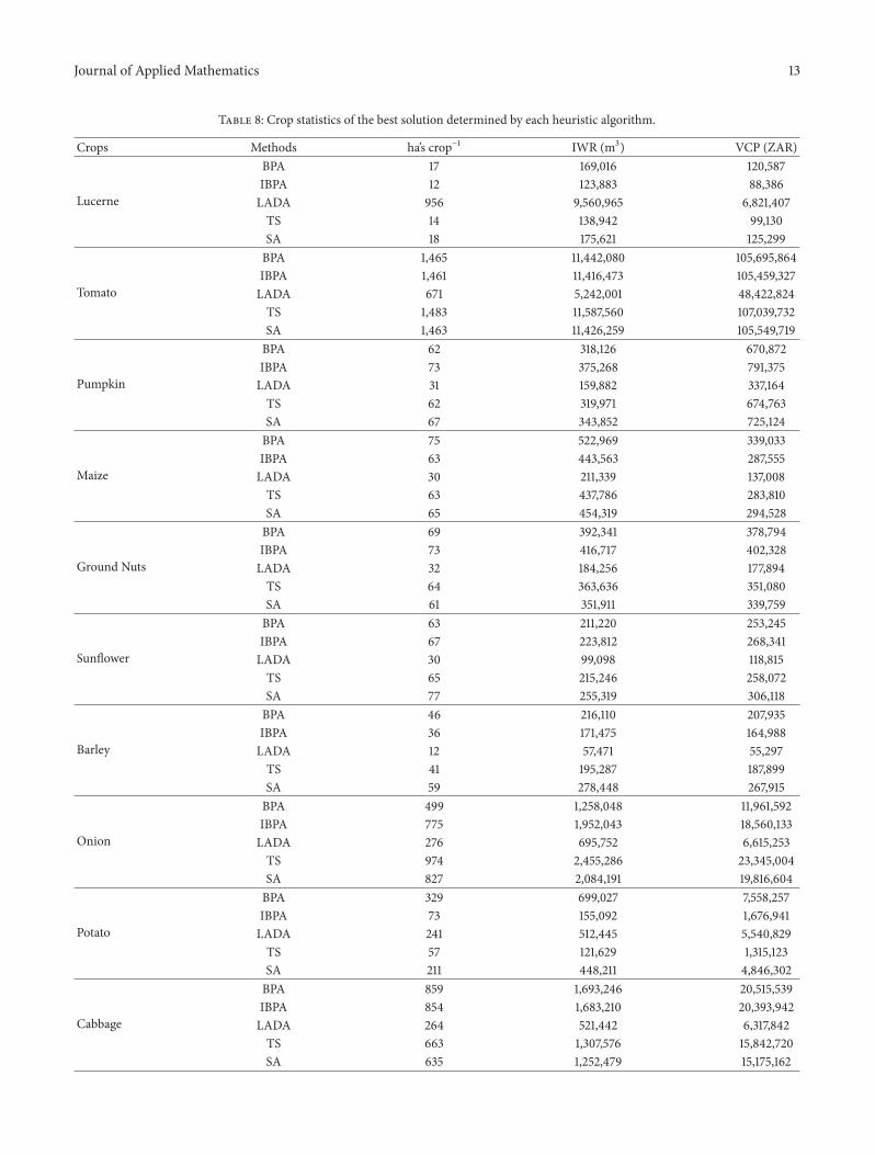When an area of land gets allocated for the developmentof a new Irrigation Scheme and it has been finalized whichcrops will be cultivated then solutions need to be foundconcerning the hectare allocations amongst the competingcrops In determining the hectare allocations it needs tobe considered that different types of crops grow in differentseasons grow for different lengths of time and have differentplant requirementsThese factorsmust be considered in orderto determine feasible solutions

The problem of trying to optimize the seasonal hectareallocations of a given area of agricultural land amongstthe various competing crops that are required to be grownwithin a year is an NP-hard-type optimization problem inagricultural planning called Annual Crop Planning (ACP)ACP aims at determining solutions that seek to maximizethe total gross profits that can be earned from a given areaof agricultural land in making the most efficient uses ofthe limited resources available for agricultural productionLimited resources include land irrigated water supply andthe various costs associated with agricultural productionThesolutions found must satisfy the multiple land and irrigationwater allocation constraints that are associated with ACP inorder to be feasible

This research introduces a new Annual Crop Planningmathematical model The model has been formulated by theauthors of this paper It is intended to be used to determinesolutions to the ACP problem at a new Irrigation Scheme

Previous studies in crop and irrigation planning haveused both single and multiobjective mathematical mod-els Many optimization techniques have been used to pro-vide solutions to these models These include Linear Pro-gramming (LP) Simulated Annealing (SA) Particle SwarmOptimization (PSO) and Evolutionary Algorithms (EArsquos)amongst others

Pant et al [3] employed the Differential Evolution (DE)algorithm to provide solutions to a crop planning problemunder adequate normal and limited irrigated water supplyThe objective was to maximize the net benefits gained underthese conditions It was found that DE performed better thanthe programming tool LINGO In [4] Pant et al investigatedthe performances of four EArsquos in providing solutions to a cropplanning problem These algorithms included the GeneticAlgorithm (GA) PSO DE and Evolutionary Programming(EP) Solutions were also determined using LINGO Thesolutions found showed that from all heuristic algorithmsGA performed poorly and that DE PSO and EP were allcomparable Georgiou and Papamichail [5] used SA in com-bination with the Stochastic Gradient Descent Algorithm todetermine solutions concerning the optimized water releasepolicies of a reservoir The released water needed to beallocated efficiently amongst the various crops being grownTo maximize profits the ldquooptimalrdquo cropping pattern neededto be determined Wardlaw and Bhaktikul [6] used GA tosolve a problem of irrigated water scheduling using a 0-1 approach The research found that GA performed wellin being able to distribute irrigated water to several farmplots in satisfying the soil moisture content levels underwater stress conditionsThe water allocations were done on arotational basis Sarker andRay [7] proposed an improved EA

known as theMultiobjective Constrained Algorithm (MCA)MCA was used to provide solutions to a multiobjective cropplanning problem The research found that MCA performedrelatively better compared to the two other optimization tech-niques used These techniques included the 120576-constrainedmethod and the Nondominated Sorting Genetic Algorithm(NSGAII) Raju and Kumar [8] compared the performancesof GA and LP in providing solutions to a crop planningproblem The objective was to maximize the net benefitsgainedThe performances of GA and LP were relatively closeIt was concluded that GA is an effective heuristic algorithmthat can be used for irrigation planning Reddy andKumar [9]studied the effectiveness of using Elitism-Mutation ParticleSwarm Optimization (EMPSO) in determining the short-term release policies of irrigated water from a reservoirunder water scarce conditions The study concluded thatthe heuristic algorithm is effective in providing short-termsolutions for multicrop irrigation

This research introduces three new local search (LS)metaheuristic algorithms in the literature These algorithmsare called the Best Performance Algorithm (BPA) the Iter-ative Best Performance Algorithm (IBPA) and the LargestAbsolute Difference Algorithm (LADA) These algorithmsare used to provide solutions to an ACP problem at a newIrrigation Scheme To determine the relative merits of thesolutions provided by these algorithms their solutions havebeen compared against the solutions of two traditional LSmetaheuristic algorithms in the literature These popularmetaheuristic algorithms are Tabu Search (TS) and SimulatedAnnealing (SA) The solutions determined and comparisonsmade will indicate the possible strengths andor weaknessesof the LS algorithms in determining solutions to this ACPproblem The solutions found will be valuable in makingsuggestions concerning the seasonal hectare allocations forthe crops that are required to be grown

The rest of this paper is structured as follows Section 2describes and presents the formulation of the ACP mathe-maticalmodel Section 3 describes the case study of theTaungIrrigation Scheme Section 4 describes the SI metaheuristicalgorithms used Section 5 presents and discusses the experi-mental results obtained Finally Section 6 draws conclusionsand outlines possible future work

2 The Annual Crop PlanningMathematical Model

This Annual Crop Planning (ACP) mathematical model hasbeen formulated by the authors of this paper It is intended tobe used to determine solutions to the Annual Crop Planningproblem at a new Irrigation Scheme The feasible solutionsfound must allocate the limited amount of agricultural landamongst the various competing crops that are required tobe grown within the year These solutions must satisfy allthe constraints associated with the objective function Theobjective in determining an optimal solution is to maximizethe total gross profits that can be earned in making themost efficient usage of the limited resources available Thelimited resources include land irrigated water supply and






21 Indices






on plot 119896

22 Input Parameters
















3=






119896 (119862119896119894119895 = 119874119896119894119895 + 119862 119868119877119896119894119894119895)


24 Variables




119891 =

119897

sum

119896=1

119873119896

sum

119894=1

119872119896119894

sum

119895=1

119883119896119894119895119861119896119894119895 (1)






119871119887 119875119896 le 119871119896 le 119880119887119875119896 forall119896 119894 119895 (2)


119897

sum

119896=1

119871119896 le 119879 (3)


119872119896119894

sum

119895

119883119896119894119895 le 119871119896 forall119896 119894 (4)


119871119887119896119894119895 le 119883119896119894119895 le 119880119887119896119894119895 forall119896 119894 119895 (5)


sum

119896

sum

119894

sum

119895

119868119877119896119894119895 le 119879119860 (6)


119861119896119894119895 gt 0 forall119896 119894 119895 (7)

3 Case Study











4 Methodology



















119875119871 119865119894119905119899119890119904119904





119886then


(852) 119908119900119903119896119894119899119892 = 119875119871119894119899119889119890119909


Algorithm 1















119875119871 119865119894119905119899119890119904119904






eg Random[0 119897119894119904119905119878119894119911119890](74) 119888119906119903119903119890119899119905 = 119875119871119894119899119889119890119909 (119888119906119903119903119890119899119905119894 = 119888119906119903119903119890119899119905119894minus1)

(8) end for(9) return1198751198710

Algorithm 2

minus6 minus1 0 1 6119909 119910

|119909minus 119910|

R




1003816100381610038161003816119909 minus 119910

1003816100381610038161003816=

(119909 minus 119910) if (119909 minus 119910) ge 0


(8)





119889119896 =

10038161003816100381610038161003816119909119894119896 minus 119909119895119896

10038161003816100381610038161003816

for 119896 = 1 119901 (9)


119894and 119909

1015840




119894and119908119900119903119896119894119899119892

119895 Using119908119900119903119896119894119899119892

119894




119894and119908119900119903119896119894119899119892

119895 If119908119900119903119896119894119899119892




by119908119900119903119896119894119899119892119895 If119908119900119903119896119894119899119892

119894or119908119900119903119896119894119899119892

119895improves on 119887119890119904119905 then


119894and119908119900119903119896119894119899119892







119878119871 119865119894119905119899119890119904119904


119878119871 119865119894119905119899119890119904119904


(1198941198991198891198901199091 = 1198941198991198891198901199092)(63)119908119900119903119896119894119899119892 1 = 1198781198711198941198991198891198901199091

(64)119908119900119903119896119894119899119892 2 = 1198781198711198941198991198891198901199092

(65) 119889 = 1003816100381610038161003816119908119900119903119896119894119899119892 1 minus 119908119900119903119896119894119899119892 2

1003816100381610038161003816

(66) Perform LS (119908119900119903119896119894119899119892 1 119908119900119903119896119894119899119892 2 119889119898)

(67)119891 119908119900119903119896119894119899119892 1 = Evaluate (119908119900119903119896119894119899119892 1)

(68)119891 119908119900119903119896119894119899119892 2 = Evaluate (119908119900119903119896119894119899119892 2)


(692) 119878119871 1198651198941199051198991198901199041199041198941198991198891198901199091 = 119891 119908119900119903119896119894119899119892 1


(6932)119891 119887119890119904119905 = 119891 119908119900119903119896119894119899119892 1


(6111) 1198781198711198941198991198891198901199092 = 119908119900119903119896119894119899119892 2

(6112) 119878119871 1198651198941199051198991198901199041199041198941198991198891198901199092 = 119891 119908119900119903119896119894119899119892 2


(61132)119891 119887119890119904119905 = 119891 119908119900119903119896119894119899119892 2


(7) end for(8) return 119887119890119904119905

Algorithm 3






(2) Set 119888119906119903119903119890119899119905 = 119887119890119904119905





(841)119891 119887119890119904119905 = 119891 119888119906119903119903119890119899119905

(842) 119887119890119904119905 = 119888119906119903119903119890119899119905


(9) end for(10) return 119887119890119904119905

Algorithm 4










(2) Set 119888119906119903119903119890119899119905 = 119908119900119903119896119894119899119892 = 119887119890119904119905





(6131) 119906119904119890 119904119900119897119906119905119894119900119899 = true(614) else


(61421) 119906119904119890 119904119900119897119906119905119894119900119899 = true(6143) end if

(615) end else(616) if 119906119904119890 119904119900119897119906119905119894119900119899 then

(6161) 119906119904119890 119904119900119897119906119905119894119900119899 = false(6162)119891 119888119906119903119903119890119899119905 = 119891 119908119900119903119896119894119899119892


(61641) 119887119890119904119905 = 119888119906119903119903119890119899119905

(61642)119891 119887119890119904119905 = 119891 119888119906119903119903119890119899119905



(7) end while(8) return 119887119890119904119905

Algorithm 5












Crops 119871119887119896119894119895 119880119887119896119894119895 119865119896119894119895 119862 119868119877119896119894119895 119874119896119894119895






119894 for 119894 = 1 100 Then









120130140150160170180190200210220230240

BPA IBPA LADA TS SA

Exec

utio

n tim

e (m

s)


Avg









0275

028

0285

029

0295

03

BPA IBPA LADA TS SA

Fitn

ess v

alue

s (ZA

Rbi

llion

)


ABFVBFV







010125

0150175

020225

0250275

030325

1 2 3 4 5 6 7 8 9 10

Fitn

ess v

alue

s (ZA

Rbi

llion

)


BPAIBPALADA

TSSA








00169001695

0017001705

00171001715

00172001725

00173

BPA IBPA LADA TS SA


IWR

Volu

me (

m3b

illio

n)









0066007600860096010601160126013601460156

BPA IBPA LADA TS SA

(ZA

Rbi

llion

)


VCP








6 Conclusion


0200400600800

1000120014001600

Hec

tare

s


BPAIBPALADA

TSSA

Luce

rne

Gn

uts

Pota

to

Tom

ato

Sflo

wer

Cabb

age

Pum

pkin

Barle

y

Mai

ze

Oni

on











Lucerne


Tomato


Pumpkin


Maize


Ground Nuts


Sunflower


Barley


Onion


Potato


Cabbage









References



























Volume 2014




Journal of











Journal of


Function Spaces






Algebra







Volume 2014








21 Indices






on plot 119896

22 Input Parameters
















3=






119896 (119862119896119894119895 = 119874119896119894119895 + 119862 119868119877119896119894119894119895)


24 Variables




119891 =

119897

sum

119896=1

119873119896

sum

119894=1

119872119896119894

sum

119895=1

119883119896119894119895119861119896119894119895 (1)






119871119887 119875119896 le 119871119896 le 119880119887119875119896 forall119896 119894 119895 (2)


119897

sum

119896=1

119871119896 le 119879 (3)


119872119896119894

sum

119895

119883119896119894119895 le 119871119896 forall119896 119894 (4)


119871119887119896119894119895 le 119883119896119894119895 le 119880119887119896119894119895 forall119896 119894 119895 (5)


sum

119896

sum

119894

sum

119895

119868119877119896119894119895 le 119879119860 (6)


119861119896119894119895 gt 0 forall119896 119894 119895 (7)

3 Case Study











4 Methodology



















119875119871 119865119894119905119899119890119904119904





119886then


(852) 119908119900119903119896119894119899119892 = 119875119871119894119899119889119890119909


Algorithm 1















119875119871 119865119894119905119899119890119904119904






eg Random[0 119897119894119904119905119878119894119911119890](74) 119888119906119903119903119890119899119905 = 119875119871119894119899119889119890119909 (119888119906119903119903119890119899119905119894 = 119888119906119903119903119890119899119905119894minus1)

(8) end for(9) return1198751198710

Algorithm 2

minus6 minus1 0 1 6119909 119910

|119909minus 119910|

R




1003816100381610038161003816119909 minus 119910

1003816100381610038161003816=

(119909 minus 119910) if (119909 minus 119910) ge 0


(8)





119889119896 =

10038161003816100381610038161003816119909119894119896 minus 119909119895119896

10038161003816100381610038161003816

for 119896 = 1 119901 (9)


119894and 119909

1015840




119894and119908119900119903119896119894119899119892

119895 Using119908119900119903119896119894119899119892

119894




119894and119908119900119903119896119894119899119892

119895 If119908119900119903119896119894119899119892




by119908119900119903119896119894119899119892119895 If119908119900119903119896119894119899119892

119894or119908119900119903119896119894119899119892

119895improves on 119887119890119904119905 then


119894and119908119900119903119896119894119899119892







119878119871 119865119894119905119899119890119904119904


119878119871 119865119894119905119899119890119904119904


(1198941198991198891198901199091 = 1198941198991198891198901199092)(63)119908119900119903119896119894119899119892 1 = 1198781198711198941198991198891198901199091

(64)119908119900119903119896119894119899119892 2 = 1198781198711198941198991198891198901199092

(65) 119889 = 1003816100381610038161003816119908119900119903119896119894119899119892 1 minus 119908119900119903119896119894119899119892 2

1003816100381610038161003816

(66) Perform LS (119908119900119903119896119894119899119892 1 119908119900119903119896119894119899119892 2 119889119898)

(67)119891 119908119900119903119896119894119899119892 1 = Evaluate (119908119900119903119896119894119899119892 1)

(68)119891 119908119900119903119896119894119899119892 2 = Evaluate (119908119900119903119896119894119899119892 2)


(692) 119878119871 1198651198941199051198991198901199041199041198941198991198891198901199091 = 119891 119908119900119903119896119894119899119892 1


(6932)119891 119887119890119904119905 = 119891 119908119900119903119896119894119899119892 1


(6111) 1198781198711198941198991198891198901199092 = 119908119900119903119896119894119899119892 2

(6112) 119878119871 1198651198941199051198991198901199041199041198941198991198891198901199092 = 119891 119908119900119903119896119894119899119892 2


(61132)119891 119887119890119904119905 = 119891 119908119900119903119896119894119899119892 2


(7) end for(8) return 119887119890119904119905

Algorithm 3






(2) Set 119888119906119903119903119890119899119905 = 119887119890119904119905





(841)119891 119887119890119904119905 = 119891 119888119906119903119903119890119899119905

(842) 119887119890119904119905 = 119888119906119903119903119890119899119905


(9) end for(10) return 119887119890119904119905

Algorithm 4










(2) Set 119888119906119903119903119890119899119905 = 119908119900119903119896119894119899119892 = 119887119890119904119905





(6131) 119906119904119890 119904119900119897119906119905119894119900119899 = true(614) else


(61421) 119906119904119890 119904119900119897119906119905119894119900119899 = true(6143) end if

(615) end else(616) if 119906119904119890 119904119900119897119906119905119894119900119899 then

(6161) 119906119904119890 119904119900119897119906119905119894119900119899 = false(6162)119891 119888119906119903119903119890119899119905 = 119891 119908119900119903119896119894119899119892


(61641) 119887119890119904119905 = 119888119906119903119903119890119899119905

(61642)119891 119887119890119904119905 = 119891 119888119906119903119903119890119899119905



(7) end while(8) return 119887119890119904119905

Algorithm 5












Crops 119871119887119896119894119895 119880119887119896119894119895 119865119896119894119895 119862 119868119877119896119894119895 119874119896119894119895






119894 for 119894 = 1 100 Then









120130140150160170180190200210220230240

BPA IBPA LADA TS SA

Exec

utio

n tim

e (m

s)


Avg









0275

028

0285

029

0295

03

BPA IBPA LADA TS SA

Fitn

ess v

alue

s (ZA

Rbi

llion

)


ABFVBFV







010125

0150175

020225

0250275

030325

1 2 3 4 5 6 7 8 9 10

Fitn

ess v

alue

s (ZA

Rbi

llion

)


BPAIBPALADA

TSSA








00169001695

0017001705

00171001715

00172001725

00173

BPA IBPA LADA TS SA


IWR

Volu

me (

m3b

illio

n)









0066007600860096010601160126013601460156

BPA IBPA LADA TS SA

(ZA

Rbi

llion

)


VCP








6 Conclusion


0200400600800

1000120014001600

Hec

tare

s


BPAIBPALADA

TSSA

Luce

rne

Gn

uts

Pota

to

Tom

ato

Sflo

wer

Cabb

age

Pum

pkin

Barle

y

Mai

ze

Oni

on











Lucerne


Tomato


Pumpkin


Maize


Ground Nuts


Sunflower


Barley


Onion


Potato


Cabbage









References



























Volume 2014




Journal of











Journal of


Function Spaces






Algebra







Volume 2014







119871119887 119875119896 le 119871119896 le 119880119887119875119896 forall119896 119894 119895 (2)


119897

sum

119896=1

119871119896 le 119879 (3)


119872119896119894

sum

119895

119883119896119894119895 le 119871119896 forall119896 119894 (4)


119871119887119896119894119895 le 119883119896119894119895 le 119880119887119896119894119895 forall119896 119894 119895 (5)


sum

119896

sum

119894

sum

119895

119868119877119896119894119895 le 119879119860 (6)


119861119896119894119895 gt 0 forall119896 119894 119895 (7)

3 Case Study











4 Methodology



















119875119871 119865119894119905119899119890119904119904





119886then


(852) 119908119900119903119896119894119899119892 = 119875119871119894119899119889119890119909


Algorithm 1















119875119871 119865119894119905119899119890119904119904






eg Random[0 119897119894119904119905119878119894119911119890](74) 119888119906119903119903119890119899119905 = 119875119871119894119899119889119890119909 (119888119906119903119903119890119899119905119894 = 119888119906119903119903119890119899119905119894minus1)

(8) end for(9) return1198751198710

Algorithm 2

minus6 minus1 0 1 6119909 119910

|119909minus 119910|

R




1003816100381610038161003816119909 minus 119910

1003816100381610038161003816=

(119909 minus 119910) if (119909 minus 119910) ge 0


(8)





119889119896 =

10038161003816100381610038161003816119909119894119896 minus 119909119895119896

10038161003816100381610038161003816

for 119896 = 1 119901 (9)


119894and 119909

1015840




119894and119908119900119903119896119894119899119892

119895 Using119908119900119903119896119894119899119892

119894




119894and119908119900119903119896119894119899119892

119895 If119908119900119903119896119894119899119892




by119908119900119903119896119894119899119892119895 If119908119900119903119896119894119899119892

119894or119908119900119903119896119894119899119892

119895improves on 119887119890119904119905 then


119894and119908119900119903119896119894119899119892







119878119871 119865119894119905119899119890119904119904


119878119871 119865119894119905119899119890119904119904


(1198941198991198891198901199091 = 1198941198991198891198901199092)(63)119908119900119903119896119894119899119892 1 = 1198781198711198941198991198891198901199091

(64)119908119900119903119896119894119899119892 2 = 1198781198711198941198991198891198901199092

(65) 119889 = 1003816100381610038161003816119908119900119903119896119894119899119892 1 minus 119908119900119903119896119894119899119892 2

1003816100381610038161003816

(66) Perform LS (119908119900119903119896119894119899119892 1 119908119900119903119896119894119899119892 2 119889119898)

(67)119891 119908119900119903119896119894119899119892 1 = Evaluate (119908119900119903119896119894119899119892 1)

(68)119891 119908119900119903119896119894119899119892 2 = Evaluate (119908119900119903119896119894119899119892 2)


(692) 119878119871 1198651198941199051198991198901199041199041198941198991198891198901199091 = 119891 119908119900119903119896119894119899119892 1


(6932)119891 119887119890119904119905 = 119891 119908119900119903119896119894119899119892 1


(6111) 1198781198711198941198991198891198901199092 = 119908119900119903119896119894119899119892 2

(6112) 119878119871 1198651198941199051198991198901199041199041198941198991198891198901199092 = 119891 119908119900119903119896119894119899119892 2


(61132)119891 119887119890119904119905 = 119891 119908119900119903119896119894119899119892 2


(7) end for(8) return 119887119890119904119905

Algorithm 3






(2) Set 119888119906119903119903119890119899119905 = 119887119890119904119905





(841)119891 119887119890119904119905 = 119891 119888119906119903119903119890119899119905

(842) 119887119890119904119905 = 119888119906119903119903119890119899119905


(9) end for(10) return 119887119890119904119905

Algorithm 4










(2) Set 119888119906119903119903119890119899119905 = 119908119900119903119896119894119899119892 = 119887119890119904119905





(6131) 119906119904119890 119904119900119897119906119905119894119900119899 = true(614) else


(61421) 119906119904119890 119904119900119897119906119905119894119900119899 = true(6143) end if

(615) end else(616) if 119906119904119890 119904119900119897119906119905119894119900119899 then

(6161) 119906119904119890 119904119900119897119906119905119894119900119899 = false(6162)119891 119888119906119903119903119890119899119905 = 119891 119908119900119903119896119894119899119892


(61641) 119887119890119904119905 = 119888119906119903119903119890119899119905

(61642)119891 119887119890119904119905 = 119891 119888119906119903119903119890119899119905



(7) end while(8) return 119887119890119904119905

Algorithm 5












Crops 119871119887119896119894119895 119880119887119896119894119895 119865119896119894119895 119862 119868119877119896119894119895 119874119896119894119895






119894 for 119894 = 1 100 Then









120130140150160170180190200210220230240

BPA IBPA LADA TS SA

Exec

utio

n tim

e (m

s)


Avg









0275

028

0285

029

0295

03

BPA IBPA LADA TS SA

Fitn

ess v

alue

s (ZA

Rbi

llion

)


ABFVBFV







010125

0150175

020225

0250275

030325

1 2 3 4 5 6 7 8 9 10

Fitn

ess v

alue

s (ZA

Rbi

llion

)


BPAIBPALADA

TSSA








00169001695

0017001705

00171001715

00172001725

00173

BPA IBPA LADA TS SA


IWR

Volu

me (

m3b

illio

n)









0066007600860096010601160126013601460156

BPA IBPA LADA TS SA

(ZA

Rbi

llion

)


VCP








6 Conclusion


0200400600800

1000120014001600

Hec

tare

s


BPAIBPALADA

TSSA

Luce

rne

Gn

uts

Pota

to

Tom

ato

Sflo

wer

Cabb

age

Pum

pkin

Barle

y

Mai

ze

Oni

on











Lucerne


Tomato


Pumpkin


Maize


Ground Nuts


Sunflower


Barley


Onion


Potato


Cabbage









References



























Volume 2014




Journal of











Journal of


Function Spaces






Algebra







Volume 2014




















119875119871 119865119894119905119899119890119904119904





119886then


(852) 119908119900119903119896119894119899119892 = 119875119871119894119899119889119890119909


Algorithm 1















119875119871 119865119894119905119899119890119904119904






eg Random[0 119897119894119904119905119878119894119911119890](74) 119888119906119903119903119890119899119905 = 119875119871119894119899119889119890119909 (119888119906119903119903119890119899119905119894 = 119888119906119903119903119890119899119905119894minus1)

(8) end for(9) return1198751198710

Algorithm 2

minus6 minus1 0 1 6119909 119910

|119909minus 119910|

R




1003816100381610038161003816119909 minus 119910

1003816100381610038161003816=

(119909 minus 119910) if (119909 minus 119910) ge 0


(8)





119889119896 =

10038161003816100381610038161003816119909119894119896 minus 119909119895119896

10038161003816100381610038161003816

for 119896 = 1 119901 (9)


119894and 119909

1015840




119894and119908119900119903119896119894119899119892

119895 Using119908119900119903119896119894119899119892

119894




119894and119908119900119903119896119894119899119892

119895 If119908119900119903119896119894119899119892




by119908119900119903119896119894119899119892119895 If119908119900119903119896119894119899119892

119894or119908119900119903119896119894119899119892

119895improves on 119887119890119904119905 then


119894and119908119900119903119896119894119899119892







119878119871 119865119894119905119899119890119904119904


119878119871 119865119894119905119899119890119904119904


(1198941198991198891198901199091 = 1198941198991198891198901199092)(63)119908119900119903119896119894119899119892 1 = 1198781198711198941198991198891198901199091

(64)119908119900119903119896119894119899119892 2 = 1198781198711198941198991198891198901199092

(65) 119889 = 1003816100381610038161003816119908119900119903119896119894119899119892 1 minus 119908119900119903119896119894119899119892 2

1003816100381610038161003816

(66) Perform LS (119908119900119903119896119894119899119892 1 119908119900119903119896119894119899119892 2 119889119898)

(67)119891 119908119900119903119896119894119899119892 1 = Evaluate (119908119900119903119896119894119899119892 1)

(68)119891 119908119900119903119896119894119899119892 2 = Evaluate (119908119900119903119896119894119899119892 2)


(692) 119878119871 1198651198941199051198991198901199041199041198941198991198891198901199091 = 119891 119908119900119903119896119894119899119892 1


(6932)119891 119887119890119904119905 = 119891 119908119900119903119896119894119899119892 1


(6111) 1198781198711198941198991198891198901199092 = 119908119900119903119896119894119899119892 2

(6112) 119878119871 1198651198941199051198991198901199041199041198941198991198891198901199092 = 119891 119908119900119903119896119894119899119892 2


(61132)119891 119887119890119904119905 = 119891 119908119900119903119896119894119899119892 2


(7) end for(8) return 119887119890119904119905

Algorithm 3






(2) Set 119888119906119903119903119890119899119905 = 119887119890119904119905





(841)119891 119887119890119904119905 = 119891 119888119906119903119903119890119899119905

(842) 119887119890119904119905 = 119888119906119903119903119890119899119905


(9) end for(10) return 119887119890119904119905

Algorithm 4










(2) Set 119888119906119903119903119890119899119905 = 119908119900119903119896119894119899119892 = 119887119890119904119905





(6131) 119906119904119890 119904119900119897119906119905119894119900119899 = true(614) else


(61421) 119906119904119890 119904119900119897119906119905119894119900119899 = true(6143) end if

(615) end else(616) if 119906119904119890 119904119900119897119906119905119894119900119899 then

(6161) 119906119904119890 119904119900119897119906119905119894119900119899 = false(6162)119891 119888119906119903119903119890119899119905 = 119891 119908119900119903119896119894119899119892


(61641) 119887119890119904119905 = 119888119906119903119903119890119899119905

(61642)119891 119887119890119904119905 = 119891 119888119906119903119903119890119899119905



(7) end while(8) return 119887119890119904119905

Algorithm 5












Crops 119871119887119896119894119895 119880119887119896119894119895 119865119896119894119895 119862 119868119877119896119894119895 119874119896119894119895






119894 for 119894 = 1 100 Then









120130140150160170180190200210220230240

BPA IBPA LADA TS SA

Exec

utio

n tim

e (m

s)


Avg









0275

028

0285

029

0295

03

BPA IBPA LADA TS SA

Fitn

ess v

alue

s (ZA

Rbi

llion

)


ABFVBFV







010125

0150175

020225

0250275

030325

1 2 3 4 5 6 7 8 9 10

Fitn

ess v

alue

s (ZA

Rbi

llion

)


BPAIBPALADA

TSSA








00169001695

0017001705

00171001715

00172001725

00173

BPA IBPA LADA TS SA


IWR

Volu

me (

m3b

illio

n)









0066007600860096010601160126013601460156

BPA IBPA LADA TS SA

(ZA

Rbi

llion

)


VCP








6 Conclusion


0200400600800

1000120014001600

Hec

tare

s


BPAIBPALADA

TSSA

Luce

rne

Gn

uts

Pota

to

Tom

ato

Sflo

wer

Cabb

age

Pum

pkin

Barle

y

Mai

ze

Oni

on











Lucerne


Tomato


Pumpkin


Maize


Ground Nuts


Sunflower


Barley


Onion


Potato


Cabbage









References



























Volume 2014




Journal of











Journal of


Function Spaces






Algebra







Volume 2014







119875119871 119865119894119905119899119890119904119904






eg Random[0 119897119894119904119905119878119894119911119890](74) 119888119906119903119903119890119899119905 = 119875119871119894119899119889119890119909 (119888119906119903119903119890119899119905119894 = 119888119906119903119903119890119899119905119894minus1)

(8) end for(9) return1198751198710

Algorithm 2

minus6 minus1 0 1 6119909 119910

|119909minus 119910|

R




1003816100381610038161003816119909 minus 119910

1003816100381610038161003816=

(119909 minus 119910) if (119909 minus 119910) ge 0


(8)





119889119896 =

10038161003816100381610038161003816119909119894119896 minus 119909119895119896

10038161003816100381610038161003816

for 119896 = 1 119901 (9)


119894and 119909

1015840




119894and119908119900119903119896119894119899119892

119895 Using119908119900119903119896119894119899119892

119894




119894and119908119900119903119896119894119899119892

119895 If119908119900119903119896119894119899119892




by119908119900119903119896119894119899119892119895 If119908119900119903119896119894119899119892

119894or119908119900119903119896119894119899119892

119895improves on 119887119890119904119905 then


119894and119908119900119903119896119894119899119892







119878119871 119865119894119905119899119890119904119904


119878119871 119865119894119905119899119890119904119904


(1198941198991198891198901199091 = 1198941198991198891198901199092)(63)119908119900119903119896119894119899119892 1 = 1198781198711198941198991198891198901199091

(64)119908119900119903119896119894119899119892 2 = 1198781198711198941198991198891198901199092

(65) 119889 = 1003816100381610038161003816119908119900119903119896119894119899119892 1 minus 119908119900119903119896119894119899119892 2

1003816100381610038161003816

(66) Perform LS (119908119900119903119896119894119899119892 1 119908119900119903119896119894119899119892 2 119889119898)

(67)119891 119908119900119903119896119894119899119892 1 = Evaluate (119908119900119903119896119894119899119892 1)

(68)119891 119908119900119903119896119894119899119892 2 = Evaluate (119908119900119903119896119894119899119892 2)


(692) 119878119871 1198651198941199051198991198901199041199041198941198991198891198901199091 = 119891 119908119900119903119896119894119899119892 1


(6932)119891 119887119890119904119905 = 119891 119908119900119903119896119894119899119892 1


(6111) 1198781198711198941198991198891198901199092 = 119908119900119903119896119894119899119892 2

(6112) 119878119871 1198651198941199051198991198901199041199041198941198991198891198901199092 = 119891 119908119900119903119896119894119899119892 2


(61132)119891 119887119890119904119905 = 119891 119908119900119903119896119894119899119892 2


(7) end for(8) return 119887119890119904119905

Algorithm 3






(2) Set 119888119906119903119903119890119899119905 = 119887119890119904119905





(841)119891 119887119890119904119905 = 119891 119888119906119903119903119890119899119905

(842) 119887119890119904119905 = 119888119906119903119903119890119899119905


(9) end for(10) return 119887119890119904119905

Algorithm 4










(2) Set 119888119906119903119903119890119899119905 = 119908119900119903119896119894119899119892 = 119887119890119904119905





(6131) 119906119904119890 119904119900119897119906119905119894119900119899 = true(614) else


(61421) 119906119904119890 119904119900119897119906119905119894119900119899 = true(6143) end if

(615) end else(616) if 119906119904119890 119904119900119897119906119905119894119900119899 then

(6161) 119906119904119890 119904119900119897119906119905119894119900119899 = false(6162)119891 119888119906119903119903119890119899119905 = 119891 119908119900119903119896119894119899119892


(61641) 119887119890119904119905 = 119888119906119903119903119890119899119905

(61642)119891 119887119890119904119905 = 119891 119888119906119903119903119890119899119905



(7) end while(8) return 119887119890119904119905

Algorithm 5












Crops 119871119887119896119894119895 119880119887119896119894119895 119865119896119894119895 119862 119868119877119896119894119895 119874119896119894119895






119894 for 119894 = 1 100 Then









120130140150160170180190200210220230240

BPA IBPA LADA TS SA

Exec

utio

n tim

e (m

s)


Avg









0275

028

0285

029

0295

03

BPA IBPA LADA TS SA

Fitn

ess v

alue

s (ZA

Rbi

llion

)


ABFVBFV







010125

0150175

020225

0250275

030325

1 2 3 4 5 6 7 8 9 10

Fitn

ess v

alue

s (ZA

Rbi

llion

)


BPAIBPALADA

TSSA








00169001695

0017001705

00171001715

00172001725

00173

BPA IBPA LADA TS SA


IWR

Volu

me (

m3b

illio

n)









0066007600860096010601160126013601460156

BPA IBPA LADA TS SA

(ZA

Rbi

llion

)


VCP








6 Conclusion


0200400600800

1000120014001600

Hec

tare

s


BPAIBPALADA

TSSA

Luce

rne

Gn

uts

Pota

to

Tom

ato

Sflo

wer

Cabb

age

Pum

pkin

Barle

y

Mai

ze

Oni

on











Lucerne


Tomato


Pumpkin


Maize


Ground Nuts


Sunflower


Barley


Onion


Potato


Cabbage









References



























Volume 2014




Journal of











Journal of


Function Spaces






Algebra







Volume 2014





119878119871 119865119894119905119899119890119904119904


119878119871 119865119894119905119899119890119904119904


(1198941198991198891198901199091 = 1198941198991198891198901199092)(63)119908119900119903119896119894119899119892 1 = 1198781198711198941198991198891198901199091

(64)119908119900119903119896119894119899119892 2 = 1198781198711198941198991198891198901199092

(65) 119889 = 1003816100381610038161003816119908119900119903119896119894119899119892 1 minus 119908119900119903119896119894119899119892 2

1003816100381610038161003816

(66) Perform LS (119908119900119903119896119894119899119892 1 119908119900119903119896119894119899119892 2 119889119898)

(67)119891 119908119900119903119896119894119899119892 1 = Evaluate (119908119900119903119896119894119899119892 1)

(68)119891 119908119900119903119896119894119899119892 2 = Evaluate (119908119900119903119896119894119899119892 2)


(692) 119878119871 1198651198941199051198991198901199041199041198941198991198891198901199091 = 119891 119908119900119903119896119894119899119892 1


(6932)119891 119887119890119904119905 = 119891 119908119900119903119896119894119899119892 1


(6111) 1198781198711198941198991198891198901199092 = 119908119900119903119896119894119899119892 2

(6112) 119878119871 1198651198941199051198991198901199041199041198941198991198891198901199092 = 119891 119908119900119903119896119894119899119892 2


(61132)119891 119887119890119904119905 = 119891 119908119900119903119896119894119899119892 2


(7) end for(8) return 119887119890119904119905

Algorithm 3






(2) Set 119888119906119903119903119890119899119905 = 119887119890119904119905





(841)119891 119887119890119904119905 = 119891 119888119906119903119903119890119899119905

(842) 119887119890119904119905 = 119888119906119903119903119890119899119905


(9) end for(10) return 119887119890119904119905

Algorithm 4










(2) Set 119888119906119903119903119890119899119905 = 119908119900119903119896119894119899119892 = 119887119890119904119905





(6131) 119906119904119890 119904119900119897119906119905119894119900119899 = true(614) else


(61421) 119906119904119890 119904119900119897119906119905119894119900119899 = true(6143) end if

(615) end else(616) if 119906119904119890 119904119900119897119906119905119894119900119899 then

(6161) 119906119904119890 119904119900119897119906119905119894119900119899 = false(6162)119891 119888119906119903119903119890119899119905 = 119891 119908119900119903119896119894119899119892


(61641) 119887119890119904119905 = 119888119906119903119903119890119899119905

(61642)119891 119887119890119904119905 = 119891 119888119906119903119903119890119899119905



(7) end while(8) return 119887119890119904119905

Algorithm 5












Crops 119871119887119896119894119895 119880119887119896119894119895 119865119896119894119895 119862 119868119877119896119894119895 119874119896119894119895






119894 for 119894 = 1 100 Then









120130140150160170180190200210220230240

BPA IBPA LADA TS SA

Exec

utio

n tim

e (m

s)


Avg









0275

028

0285

029

0295

03

BPA IBPA LADA TS SA

Fitn

ess v

alue

s (ZA

Rbi

llion

)


ABFVBFV







010125

0150175

020225

0250275

030325

1 2 3 4 5 6 7 8 9 10

Fitn

ess v

alue

s (ZA

Rbi

llion

)


BPAIBPALADA

TSSA








00169001695

0017001705

00171001715

00172001725

00173

BPA IBPA LADA TS SA


IWR

Volu

me (

m3b

illio

n)









0066007600860096010601160126013601460156

BPA IBPA LADA TS SA

(ZA

Rbi

llion

)


VCP








6 Conclusion


0200400600800

1000120014001600

Hec

tare

s


BPAIBPALADA

TSSA

Luce

rne

Gn

uts

Pota

to

Tom

ato

Sflo

wer

Cabb

age

Pum

pkin

Barle

y

Mai

ze

Oni

on











Lucerne


Tomato


Pumpkin


Maize


Ground Nuts


Sunflower


Barley


Onion


Potato


Cabbage









References



























Volume 2014




Journal of











Journal of


Function Spaces






Algebra







Volume 2014





(2) Set 119888119906119903119903119890119899119905 = 119908119900119903119896119894119899119892 = 119887119890119904119905





(6131) 119906119904119890 119904119900119897119906119905119894119900119899 = true(614) else


(61421) 119906119904119890 119904119900119897119906119905119894119900119899 = true(6143) end if

(615) end else(616) if 119906119904119890 119904119900119897119906119905119894119900119899 then

(6161) 119906119904119890 119904119900119897119906119905119894119900119899 = false(6162)119891 119888119906119903119903119890119899119905 = 119891 119908119900119903119896119894119899119892


(61641) 119887119890119904119905 = 119888119906119903119903119890119899119905

(61642)119891 119887119890119904119905 = 119891 119888119906119903119903119890119899119905



(7) end while(8) return 119887119890119904119905

Algorithm 5












Crops 119871119887119896119894119895 119880119887119896119894119895 119865119896119894119895 119862 119868119877119896119894119895 119874119896119894119895






119894 for 119894 = 1 100 Then









120130140150160170180190200210220230240

BPA IBPA LADA TS SA

Exec

utio

n tim

e (m

s)


Avg









0275

028

0285

029

0295

03

BPA IBPA LADA TS SA

Fitn

ess v

alue

s (ZA

Rbi

llion

)


ABFVBFV







010125

0150175

020225

0250275

030325

1 2 3 4 5 6 7 8 9 10

Fitn

ess v

alue

s (ZA

Rbi

llion

)


BPAIBPALADA

TSSA








00169001695

0017001705

00171001715

00172001725

00173

BPA IBPA LADA TS SA


IWR

Volu

me (

m3b

illio

n)









0066007600860096010601160126013601460156

BPA IBPA LADA TS SA

(ZA

Rbi

llion

)


VCP








6 Conclusion


0200400600800

1000120014001600

Hec

tare

s


BPAIBPALADA

TSSA

Luce

rne

Gn

uts

Pota

to

Tom

ato

Sflo

wer

Cabb

age

Pum

pkin

Barle

y

Mai

ze

Oni

on











Lucerne


Tomato


Pumpkin


Maize


Ground Nuts


Sunflower


Barley


Onion


Potato


Cabbage









References



























Volume 2014




Journal of











Journal of


Function Spaces






Algebra







Volume 2014




120130140150160170180190200210220230240

BPA IBPA LADA TS SA

Exec

utio

n tim

e (m

s)


Avg









0275

028

0285

029

0295

03

BPA IBPA LADA TS SA

Fitn

ess v

alue

s (ZA

Rbi

llion

)


ABFVBFV







010125

0150175

020225

0250275

030325

1 2 3 4 5 6 7 8 9 10

Fitn

ess v

alue

s (ZA

Rbi

llion

)


BPAIBPALADA

TSSA








00169001695

0017001705

00171001715

00172001725

00173

BPA IBPA LADA TS SA


IWR

Volu

me (

m3b

illio

n)









0066007600860096010601160126013601460156

BPA IBPA LADA TS SA

(ZA

Rbi

llion

)


VCP








6 Conclusion


0200400600800

1000120014001600

Hec

tare

s


BPAIBPALADA

TSSA

Luce

rne

Gn

uts

Pota

to

Tom

ato

Sflo

wer

Cabb

age

Pum

pkin

Barle

y

Mai

ze

Oni

on











Lucerne


Tomato


Pumpkin


Maize


Ground Nuts


Sunflower


Barley


Onion


Potato


Cabbage









References



























Volume 2014




Journal of











Journal of


Function Spaces






Algebra







Volume 2014




010125

0150175

020225

0250275

030325

1 2 3 4 5 6 7 8 9 10

Fitn

ess v

alue

s (ZA

Rbi

llion

)


BPAIBPALADA

TSSA








00169001695

0017001705

00171001715

00172001725

00173

BPA IBPA LADA TS SA


IWR

Volu

me (

m3b

illio

n)









0066007600860096010601160126013601460156

BPA IBPA LADA TS SA

(ZA

Rbi

llion

)


VCP








6 Conclusion


0200400600800

1000120014001600

Hec

tare

s


BPAIBPALADA

TSSA

Luce

rne

Gn

uts

Pota

to

Tom

ato

Sflo

wer

Cabb

age

Pum

pkin

Barle

y

Mai

ze

Oni

on











Lucerne


Tomato


Pumpkin


Maize


Ground Nuts


Sunflower


Barley


Onion


Potato


Cabbage









References



























Volume 2014




Journal of











Journal of


Function Spaces






Algebra







Volume 2014




0066007600860096010601160126013601460156

BPA IBPA LADA TS SA

(ZA

Rbi

llion

)


VCP








6 Conclusion


0200400600800

1000120014001600

Hec

tare

s


BPAIBPALADA

TSSA

Luce

rne

Gn

uts

Pota

to

Tom

ato

Sflo

wer

Cabb

age

Pum

pkin

Barle

y

Mai

ze

Oni

on











Lucerne


Tomato


Pumpkin


Maize


Ground Nuts


Sunflower


Barley


Onion


Potato


Cabbage









References



























Volume 2014




Journal of











Journal of


Function Spaces






Algebra







Volume 2014






Lucerne


Tomato


Pumpkin


Maize


Ground Nuts


Sunflower


Barley


Onion


Potato


Cabbage









References



























Volume 2014




Journal of











Journal of


Function Spaces






Algebra







Volume 2014










References



























Volume 2014




Journal of











Journal of


Function Spaces






Algebra







Volume 2014










Volume 2014




Journal of











Journal of


Function Spaces






Algebra







Volume 2014



three new stochastic local search metaheuristics for …€¦ · its feasibility for agricultural...

Documents