metaheuristics neighborhood (local) search techniques
DESCRIPTION
METAHEURISTICS Neighborhood (Local) Search Techniques. Jacques A. Ferland Department of Informatique and Recherche Opérationnelle Université de Montréal [email protected]. Introduction. Introduction to some basic methods My vision relying on my experience Not an exaustive survey - PowerPoint PPT PresentationTRANSCRIPT

METAHEURISTICSNeighborhood (Local) Search Techniques
Jacques A. FerlandDepartment of Informatique and Recherche OpérationnelleUniversité de Montréal

Introduction
• Introduction to some basic methods
• My vision relying on my experience
• Not an exaustive survey
• Most of the time ad hoc adaptations of basic methods are used to deal with specific applications

Advantages of using metaheuristic
• Intuitive and easy to understand
• With regards to enduser of a real world application: - Easy to explain - Connection with the manual approach of enduser - Enduser sees easily the added features to improve the results - Allow to analyze more deeply and more scenarios
• Allow dealing with larger size problems having higher degree of complexity
• Generate rapidly very good solutions
Disadvantages of using metaheuristic
• Quick and dirty methods
• Optimality not guaranted in general
• Few convergence results for special cases

Summary
• Heuristic Constructive techniques:
Greedy
GRASP (Greedy Randomized Adaptive Search Procedure)
• Neighborhood (Local) Search Techniques:
Descent
Tabu Search
Simulated Annealing
Threshold Accepting
• Improving strategies
Intensification
Diversification
Variable Neighborhood Search (VNS)
Exchange Procedure

Problem used to illustrate
• General problemmin f(x)
x є X
• Assignment type problem: Assignment of resources j to activities i
min f(x)
Subject to ∑1≤ j≤ m xij = 1 1≤ i ≤ n
xij = 0 or 1 1≤ i ≤ n, 1≤ j ≤ m
Problem Formulation
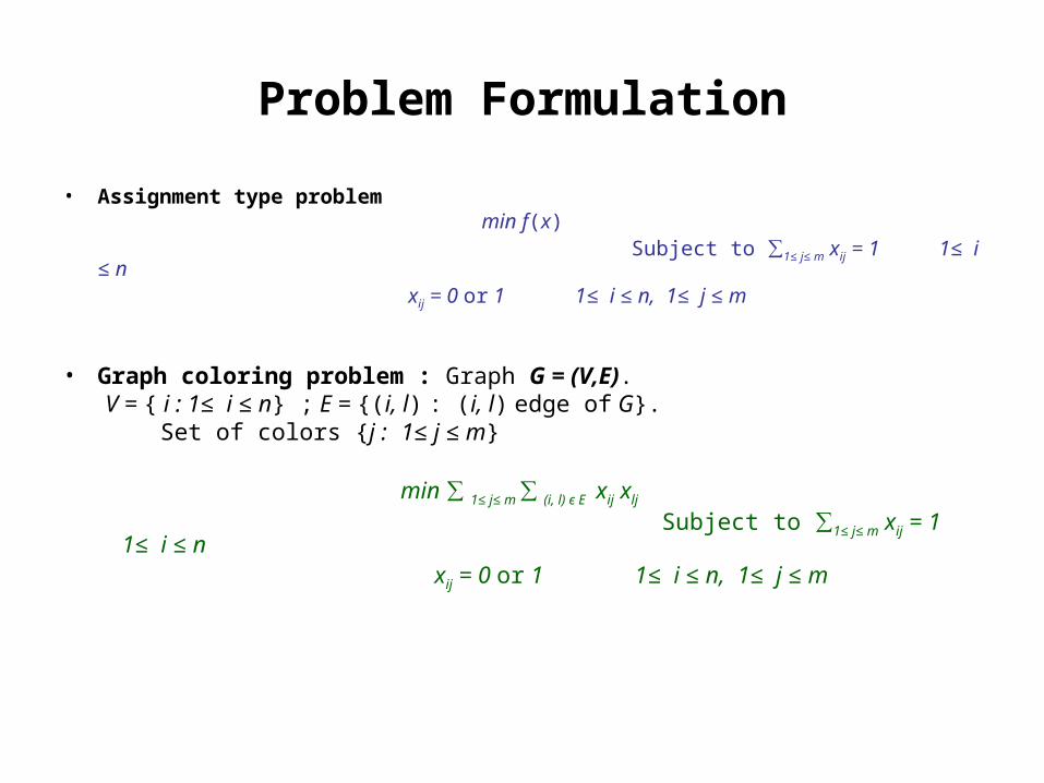
• Assignment type problemmin f(x)
Subject to ∑1≤ j≤ m xij = 1 1≤ i ≤ n xij = 0 or 1 1≤ i ≤ n, 1≤ j ≤ m
• Graph coloring problem : Graph G = (V,E). V = { i : 1≤ i ≤ n} ; E = {(i, l) : (i, l) edge of G}. Set of colors {j : 1≤ j ≤ m}
min ∑ 1≤ j≤ m ∑ (i, l) є E xij xlj Subject to ∑1≤ j≤ m xij = 1 1≤ i ≤ n xij = 0 or 1 1≤ i ≤ n, 1≤ j ≤ m

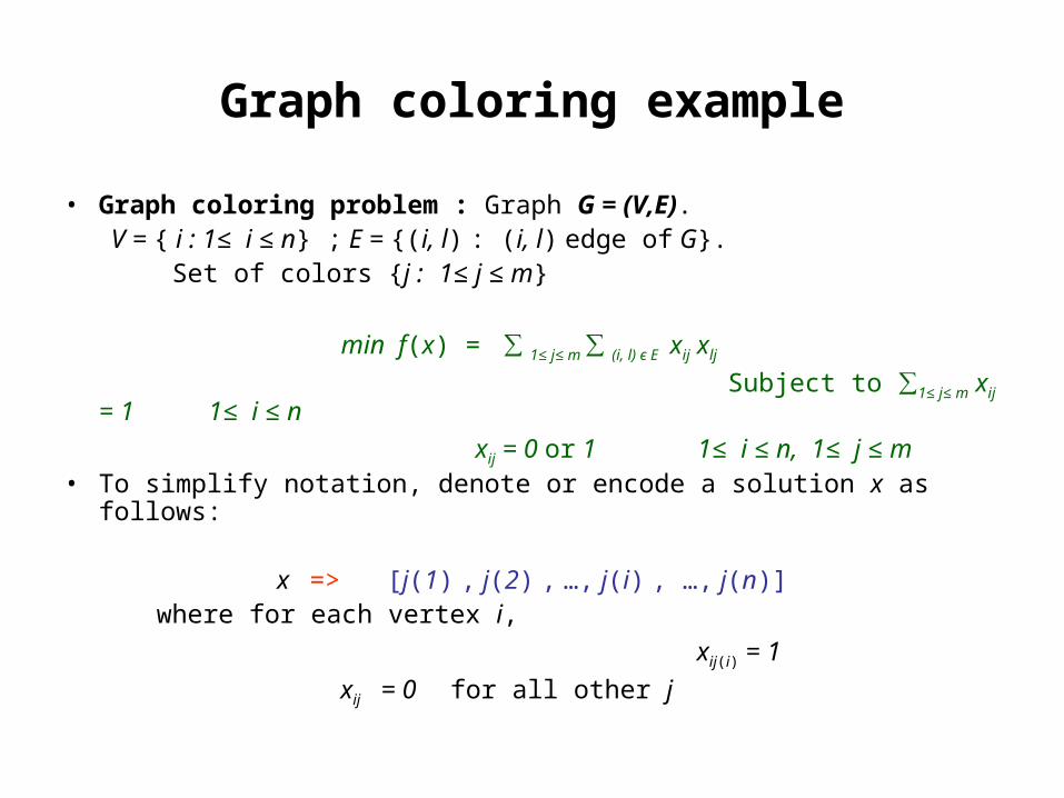
Graph coloring example
• Graph coloring problem : Graph G = (V,E). V = { i : 1≤ i ≤ n} ; E = {(i, l) : (i, l) edge of G}. Set of colors {j : 1≤ j ≤ m}
min f(x) = ∑ 1≤ j≤ m ∑ (i, l) є E xij xlj
Subject to ∑1≤ j≤ m xij = 1 1≤ i ≤ n
xij = 0 or 1 1≤ i ≤ n, 1≤ j ≤ m• To simplify notation, denote or encode a solution x as follows:
x => [j(1) , j(2) , …, j(i) , …, j(n)] where for each vertex i,
xij(i) = 1
xij = 0 for all other j

Heuristic Constructive Techniques
• Values of the variables are determined sequentially:
at each iteration, a variable is selected,
and its value is determined
• The value of each variable is never modifided once it is determined
• Techniques often used to generate initial solutions for iterative procedures
Greedy method
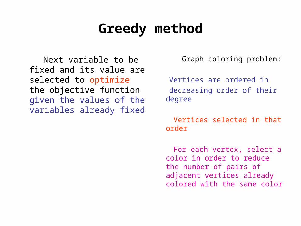
Next variable to be fixed and its value are selected to optimize the objective function given the values of the variables already fixed
Graph coloring problem:
Vertices are ordered in
decreasing order of their degree
Vertices selected in that order
For each vertex, select a color in order to reduce the number of pairs of adjacent vertices already colored with the same color
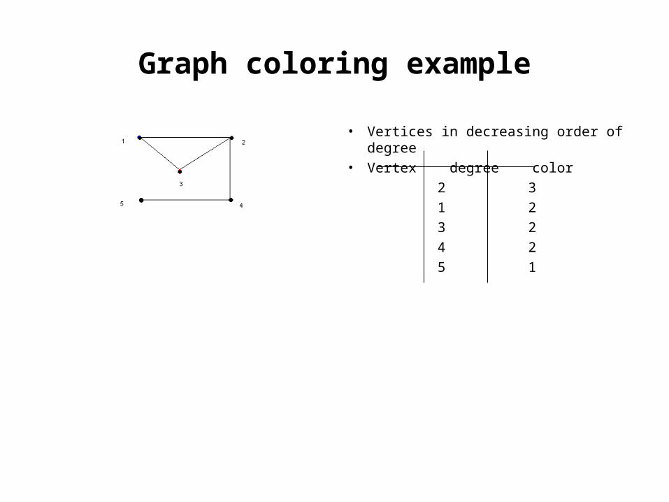
Graph coloring example
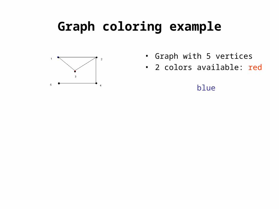
• Graph with 5 vertices
• 2 colors available: red
blue
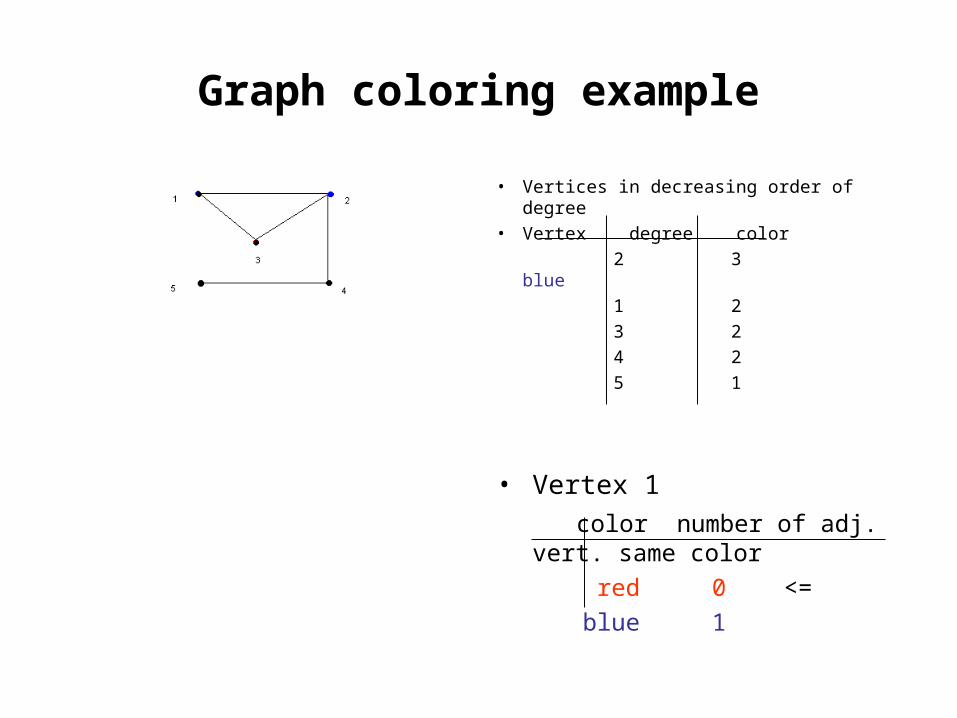
Graph coloring example
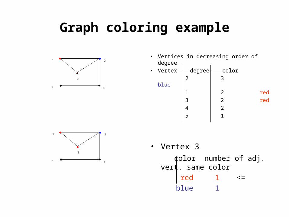
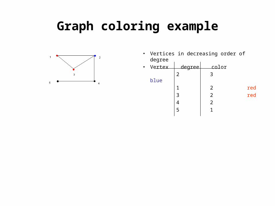
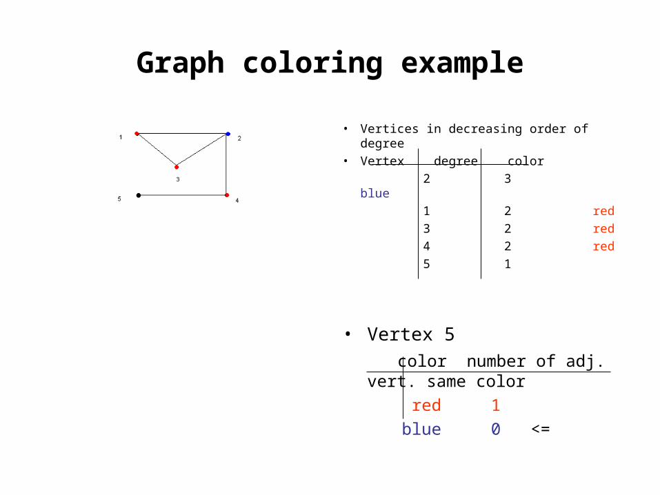
• Vertices in decreasing order of degree
• Vertex degree color
2 3
1 2
3 2
4 2
5 1
Graph coloring example
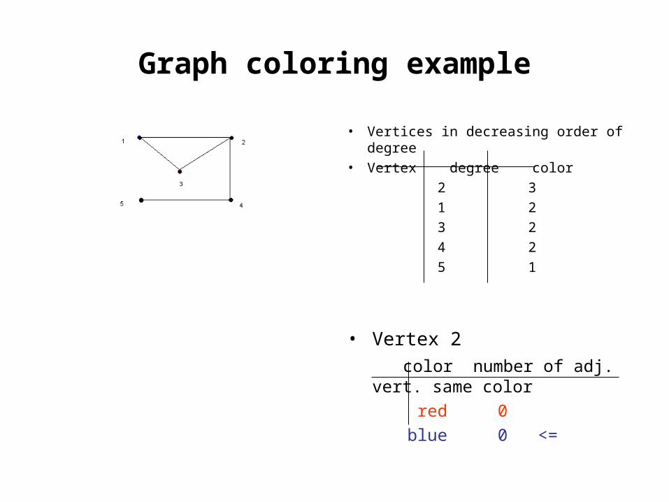
• Vertices in decreasing order of degree
• Vertex degree color
2 3
1 2
3 2
4 2
5 1
• Vertex 2
color number of adj. vert. same color
red 0
blue 0 <=
Graph coloring example
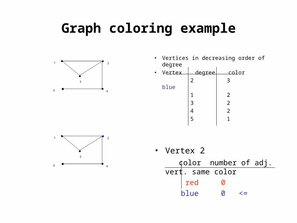
• Vertices in decreasing order of degree
• Vertex degree color
2 3 blue
1 2
3 2
4 2
5 1
• Vertex 2
color number of adj. vert. same color
red 0
blue 0 <=
Graph coloring example
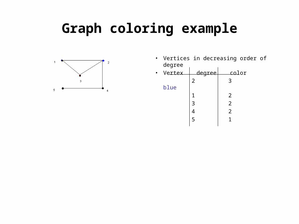
• Vertices in decreasing order of degree
• Vertex degree color
2 3 blue
1 2
3 2
4 2
5 1
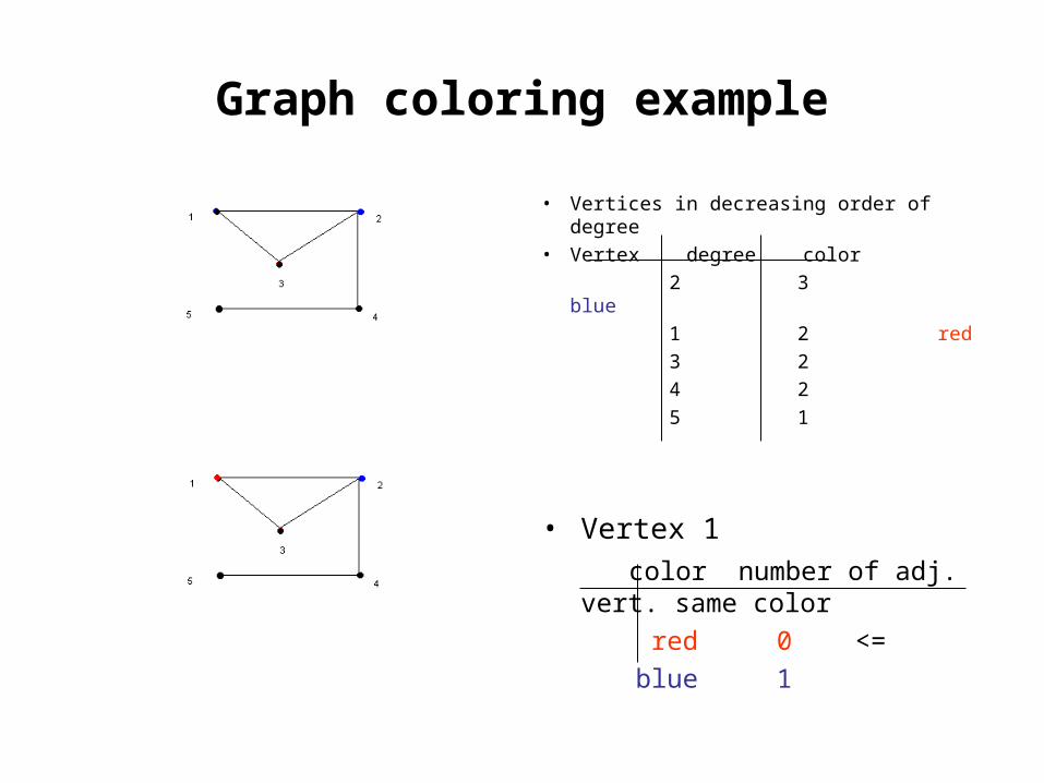
Graph coloring example
• Vertices in decreasing order of degree
• Vertex degree color
2 3 blue
1 2
3 2
4 2
5 1
• Vertex 1
color number of adj. vert. same color
red 0 <=
blue 1
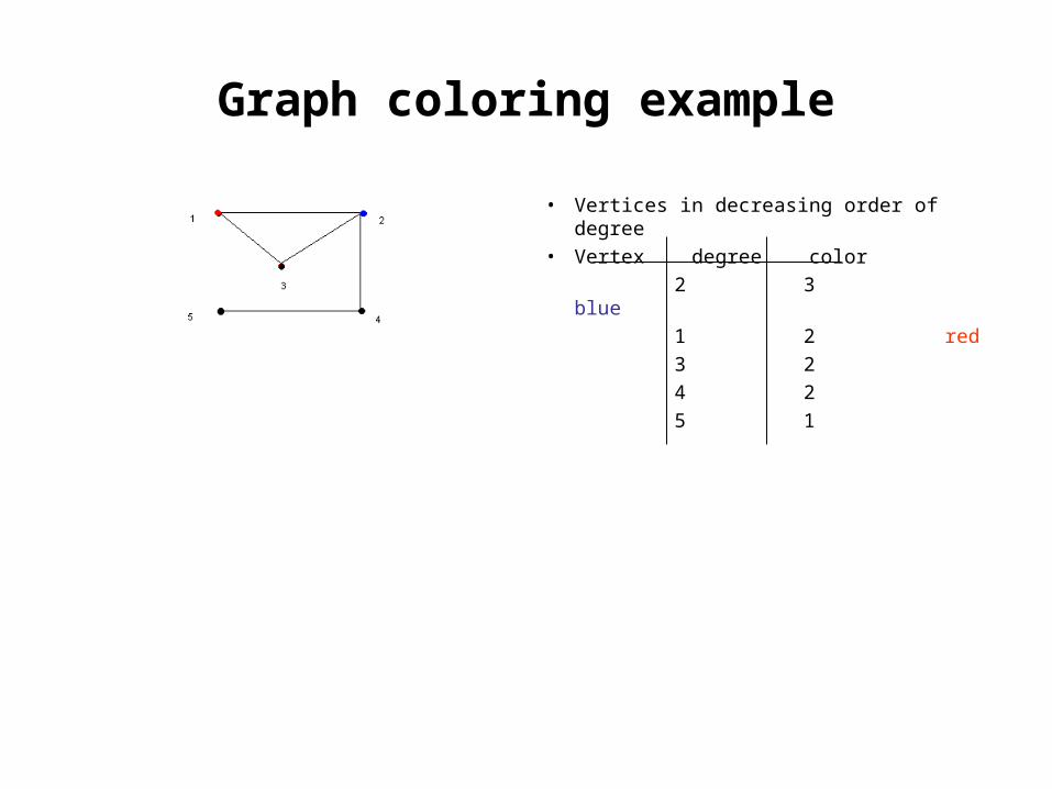
Graph coloring example
• Vertices in decreasing order of degree
• Vertex degree color
2 3 blue
1 2 red
3 2
4 2
5 1
• Vertex 1
color number of adj. vert. same color
red 0 <=
blue 1
Graph coloring example
• Vertices in decreasing order of degree
• Vertex degree color
2 3 blue
1 2 red
3 2
4 2
5 1
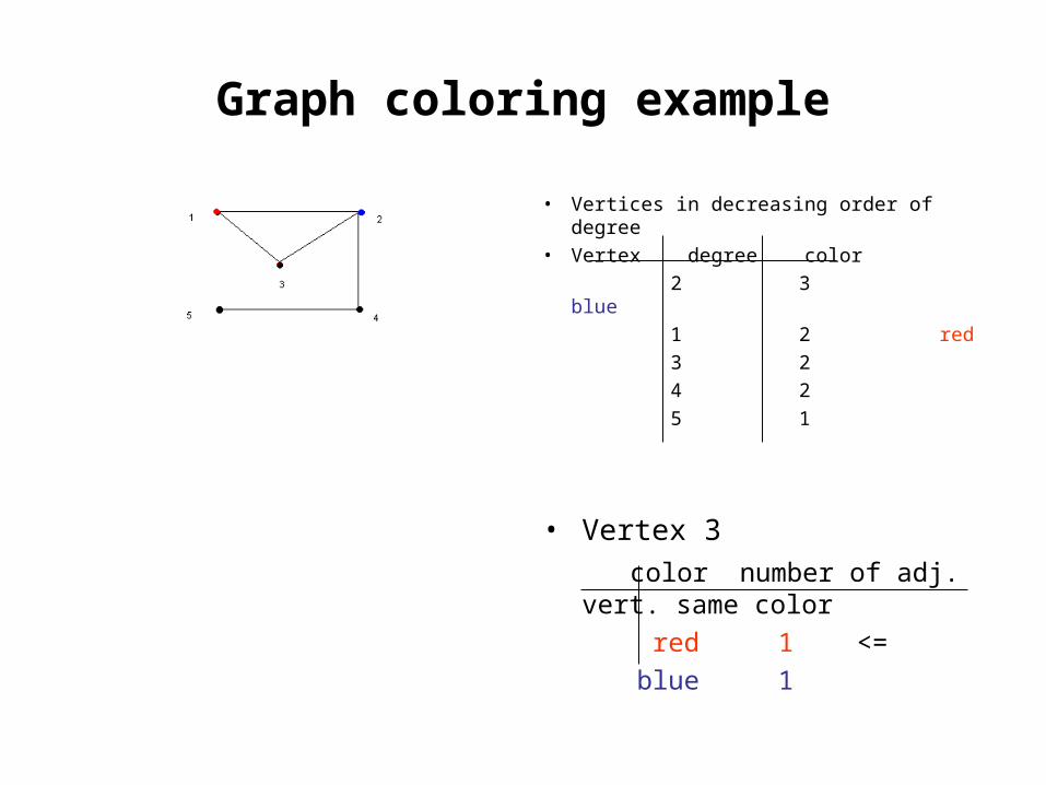
Graph coloring example
• Vertices in decreasing order of degree
• Vertex degree color
2 3 blue
1 2 red
3 2
4 2
5 1
• Vertex 3
color number of adj. vert. same color
red 1 <=
blue 1
Graph coloring example
• Vertices in decreasing order of degree
• Vertex degree color
2 3 blue
1 2 red
3 2 red
4 2
5 1
• Vertex 3
color number of adj. vert. same color
red 1 <=
blue 1
Graph coloring example
• Vertices in decreasing order of degree
• Vertex degree color
2 3 blue
1 2 red
3 2 red
4 2
5 1
Graph coloring example
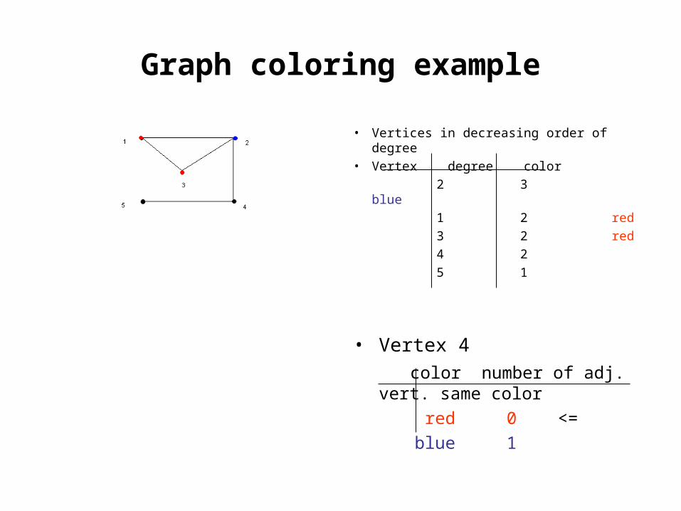
• Vertices in decreasing order of degree
• Vertex degree color
2 3 blue
1 2 red
3 2 red
4 2
5 1
• Vertex 4
color number of adj. vert. same color
red 0 <=
blue 1
Graph coloring example
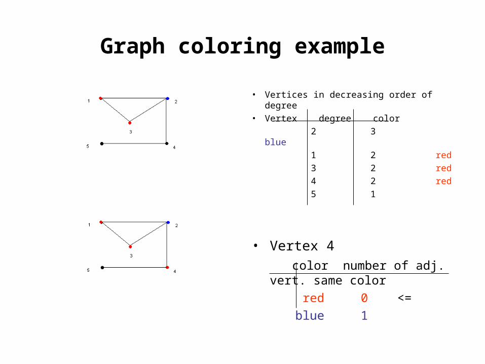
• Vertices in decreasing order of degree
• Vertex degree color
2 3 blue
1 2 red
3 2 red
4 2 red
5 1
• Vertex 4
color number of adj. vert. same color
red 0 <=
blue 1

Graph coloring example
• Vertices in decreasing order of degree
• Vertex degree color
2 3 blue
1 2 red
3 2 red
4 2 red
5 1
Graph coloring example
• Vertices in decreasing order of degree
• Vertex degree color
2 3 blue
1 2 red
3 2 red
4 2 red
5 1
• Vertex 5
color number of adj. vert. same color
red 1
blue 0 <=
Graph coloring example
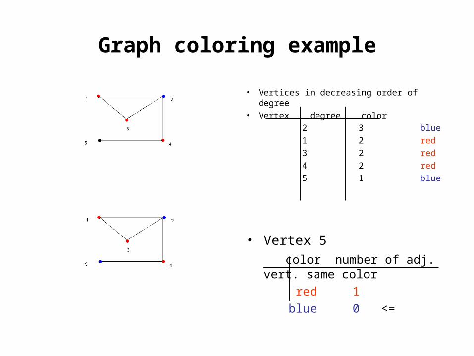
• Vertices in decreasing order of degree
• Vertex degree color
2 3 blue
1 2 red
3 2 red
4 2 red
5 1 blue
• Vertex 5
color number of adj. vert. same color
red 1
blue 0 <=
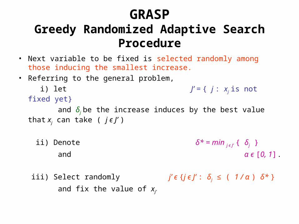
GRASPGreedy Randomized Adaptive Search Procedure
• Next variable to be fixed is selected randomly among those inducing the smallest increase.
• Referring to the general problem,
i) let J’ = { j : xj is not fixed yet}
and δj be the increase induces by the best value that xj can take ( j є J’ )
ii) Denote δ* = min j є J’ { δj }
and α є [0, 1] .
iii) Select randomly j’ є {j є J’ : δj ≤ ( 1 / α ) δ* }
and fix the value of xj’
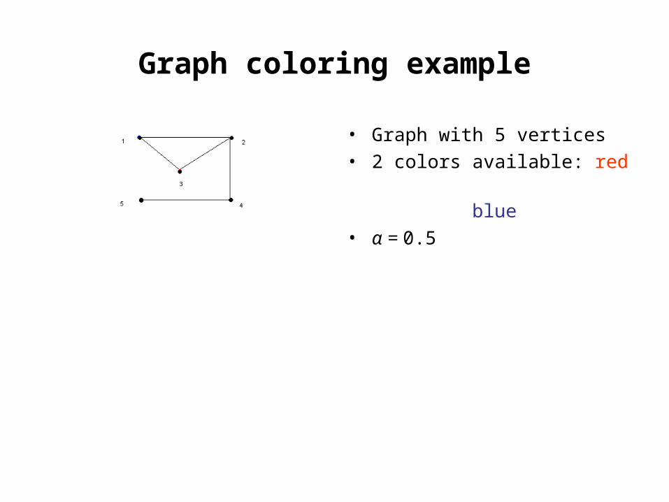
Graph coloring example
• Graph with 5 vertices
• 2 colors available: red
blue
• α = 0.5
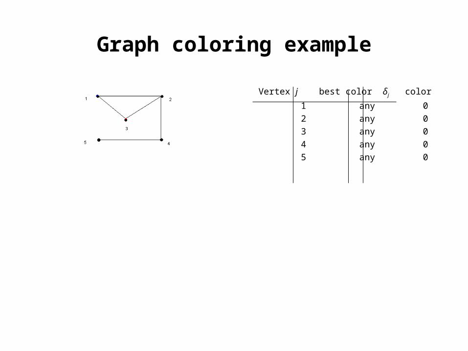
Graph coloring example
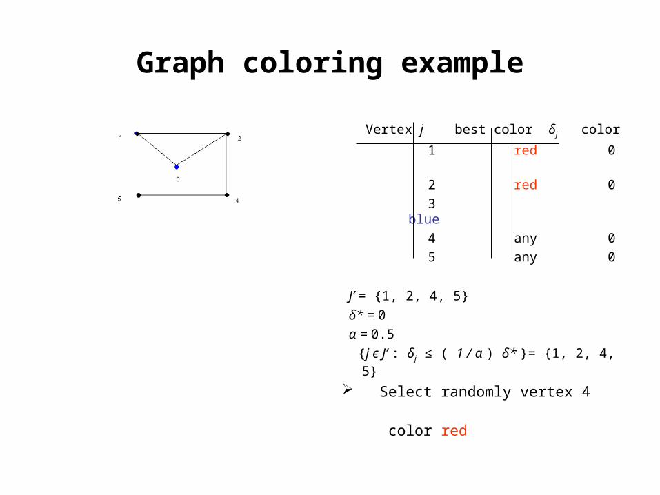
Vertex j best color δj color
1 any 0
2 any 0
3 any 0
4 any 0
5 any 0
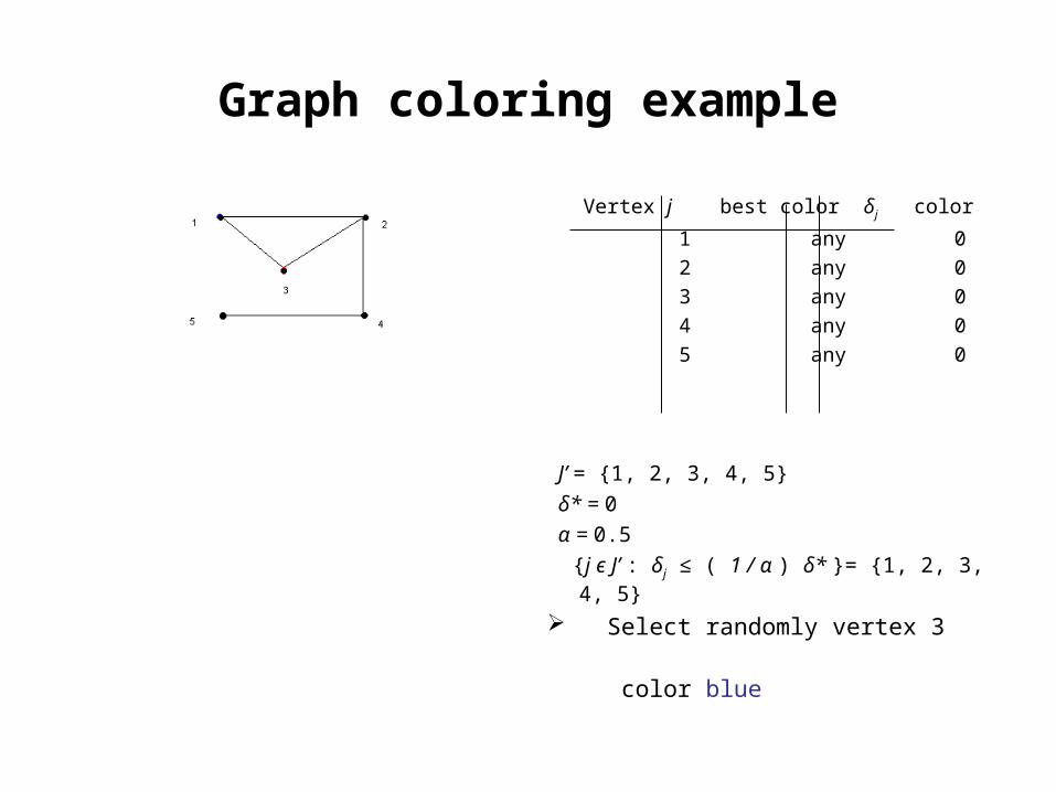
Graph coloring example
Vertex j best color δj color
1 any 0
2 any 0
3 any 0
4 any 0
5 any 0
J’ = {1, 2, 3, 4, 5}
δ* = 0
α = 0.5
{j є J’ : δj ≤ ( 1 / α ) δ* }= {1, 2, 3, 4, 5}
Select randomly vertex 3
color blue
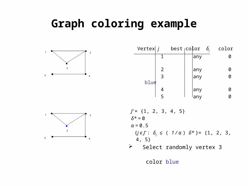
Graph coloring example
Vertex j best color δj color
1 any 0
2 any 0
3 any 0 blue
4 any 0
5 any 0
J’ = {1, 2, 3, 4, 5}
δ* = 0
α = 0.5
{j є J’ : δj ≤ ( 1 / α ) δ* }= {1, 2, 3, 4, 5}
Select randomly vertex 3
color blue
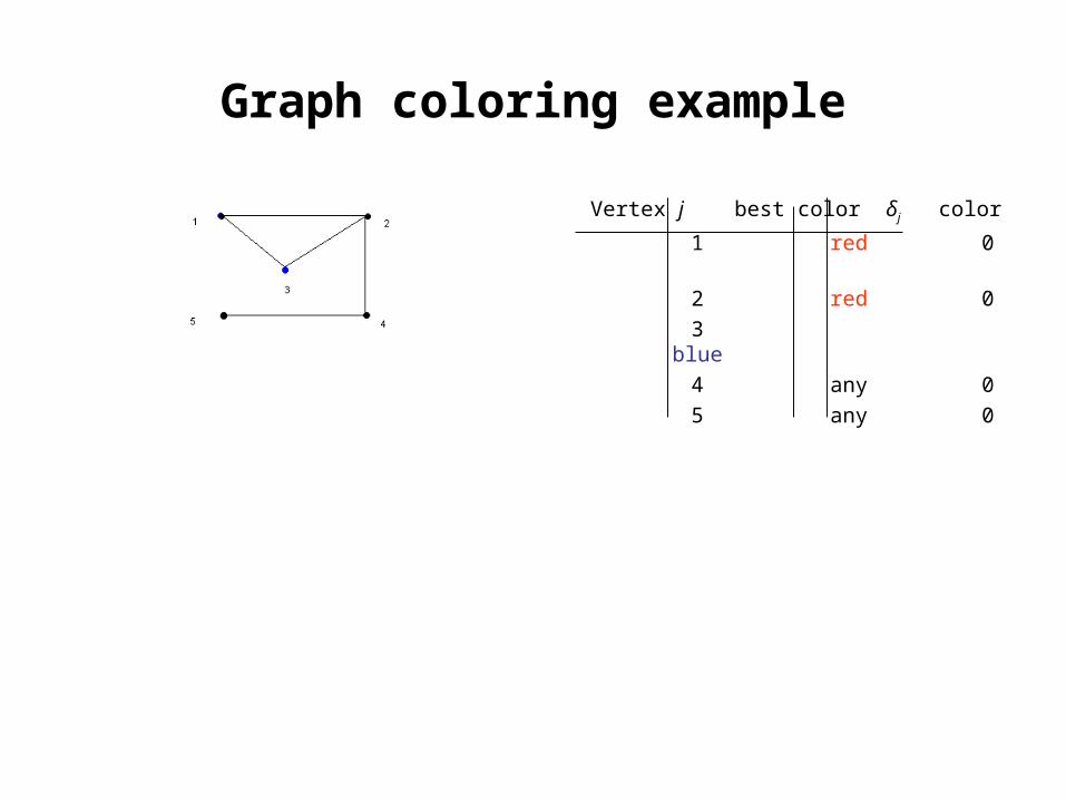
Graph coloring example
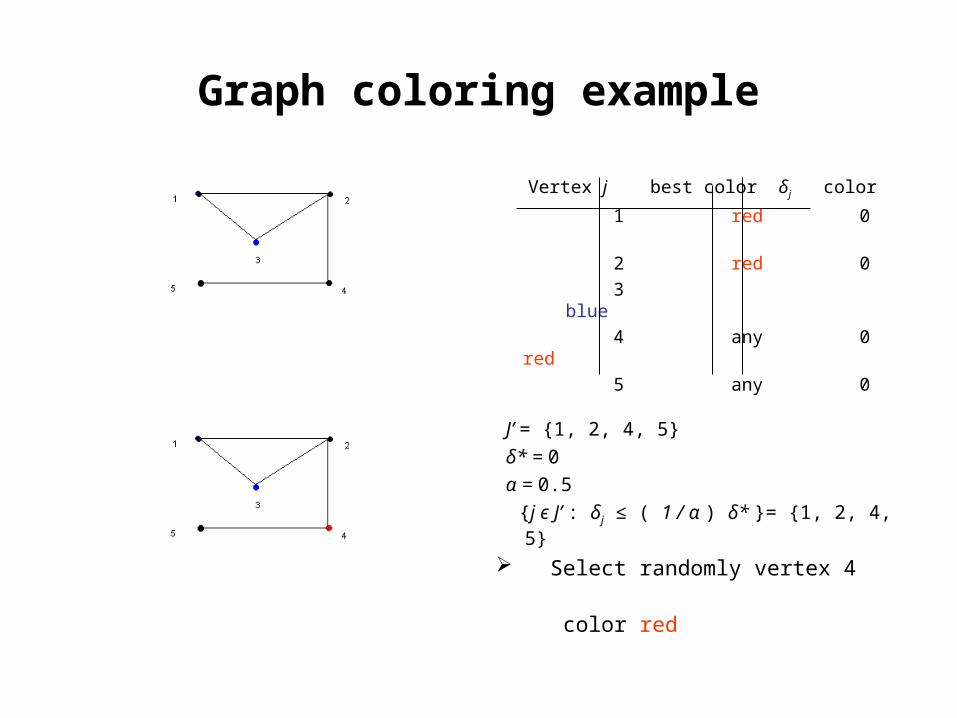
Vertex j best color δj color
1 red 0
2 red 0
3 blue
4 any 0
5 any 0
Graph coloring example
Vertex j best color δj color
1 red 0
2 red 0
3 blue
4 any 0
5 any 0
J’ = {1, 2, 4, 5}
δ* = 0
α = 0.5
{j є J’ : δj ≤ ( 1 / α ) δ* }= {1, 2, 4, 5}
Select randomly vertex 4
color red
Graph coloring example
Vertex j best color δj color
1 red 0
2 red 0
3 blue
4 any 0 red
5 any 0
J’ = {1, 2, 4, 5}
δ* = 0
α = 0.5
{j є J’ : δj ≤ ( 1 / α ) δ* }= {1, 2, 4, 5}
Select randomly vertex 4
color red
Graph coloring example
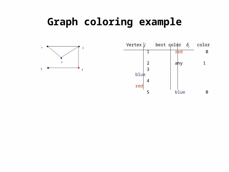
Vertex j best color δj color
1 red 0
2 any 1
3 blue
4 red
5 blue 0
Graph coloring example
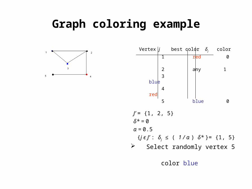
Vertex j best color δj color
1 red 0
2 any 1
3 blue
4 red
5 blue 0
J’ = {1, 2, 5}
δ* = 0
α = 0.5
{j є J’ : δj ≤ ( 1 / α ) δ* }= {1, 5}
Select randomly vertex 5
color blue
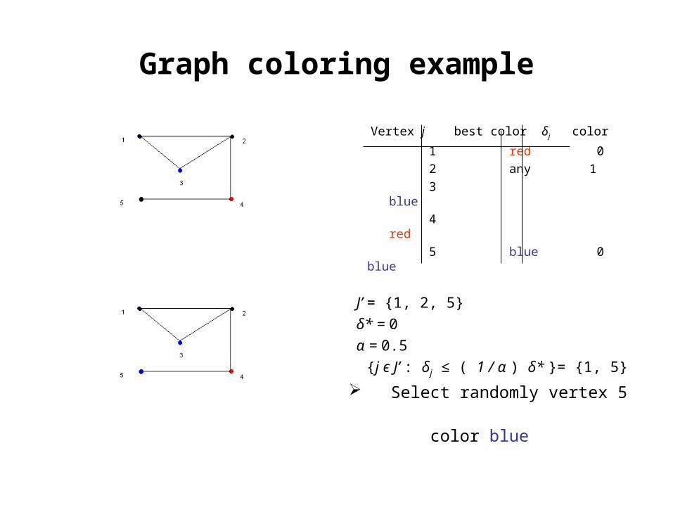
Graph coloring example
Vertex j best color δj color
1 red 0
2 any 1
3 blue
4 red
5 blue 0 blue
J’ = {1, 2, 5}
δ* = 0
α = 0.5
{j є J’ : δj ≤ ( 1 / α ) δ* }= {1, 5}
Select randomly vertex 5
color blue
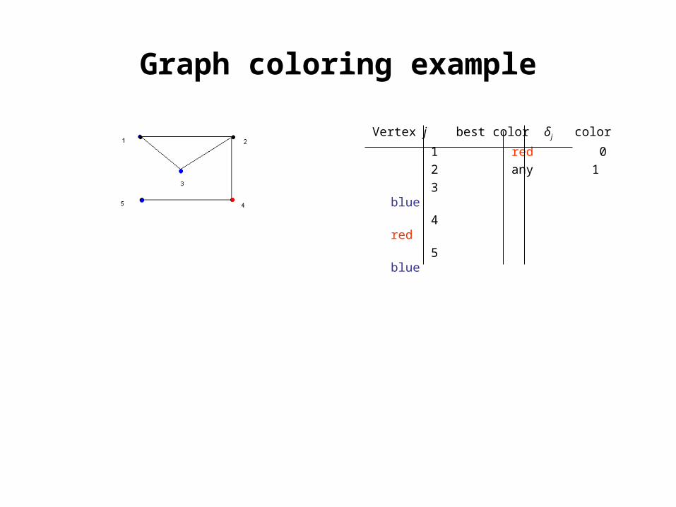
Graph coloring example
Vertex j best color δj color
1 red 0
2 any 1
3 blue
4 red
5 blue
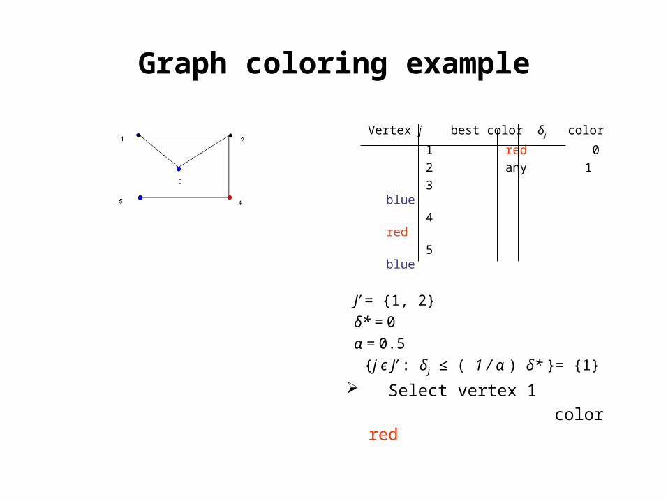
Graph coloring example
Vertex j best color δj color
1 red 0
2 any 1
3 blue
4 red
5 blue
J’ = {1, 2}
δ* = 0
α = 0.5
{j є J’ : δj ≤ ( 1 / α ) δ* }= {1}
Select vertex 1
color red
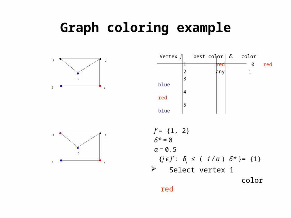
Graph coloring example
Vertex j best color δj color
1 red 0 red
2 any 1
3 blue
4 red
5 blue
J’ = {1, 2}
δ* = 0
α = 0.5
{j є J’ : δj ≤ ( 1 / α ) δ* }= {1}
Select vertex 1
color red
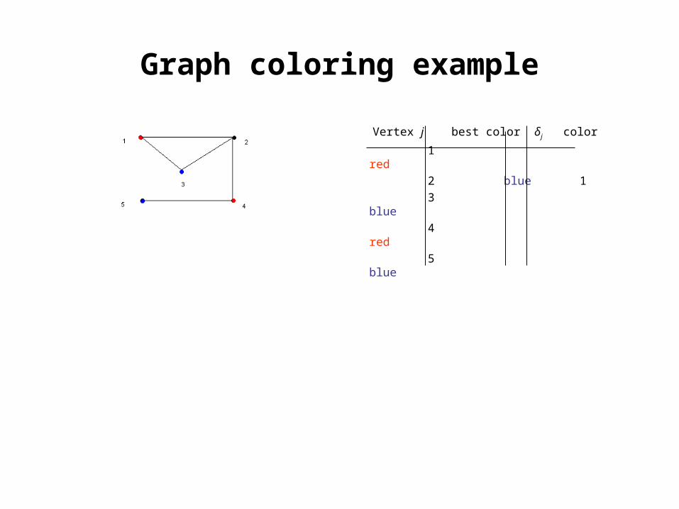
Graph coloring example
Vertex j best color δj color
1 red
2 blue 1
3 blue
4 red
5 blue
Graph coloring example
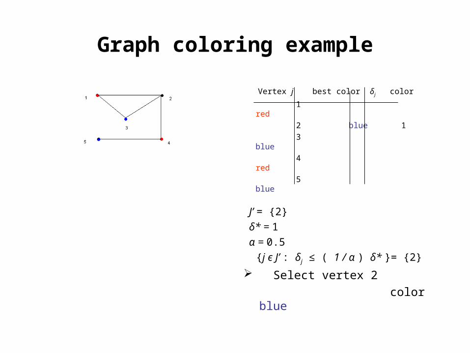
Vertex j best color δj color
1 red
2 blue 1
3 blue
4 red
5 blue
J’ = {2}
δ* = 1
α = 0.5
{j є J’ : δj ≤ ( 1 / α ) δ* }= {2}
Select vertex 2
color blue
Graph coloring example
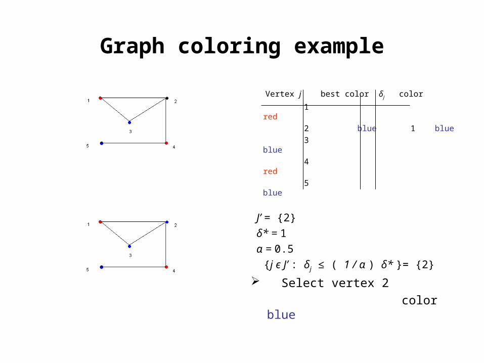
Vertex j best color δj color
1 red
2 blue 1 blue
3 blue
4 red
5 blue
J’ = {2}
δ* = 1
α = 0.5
{j є J’ : δj ≤ ( 1 / α ) δ* }= {2}
Select vertex 2
color blue
Graph coloring example
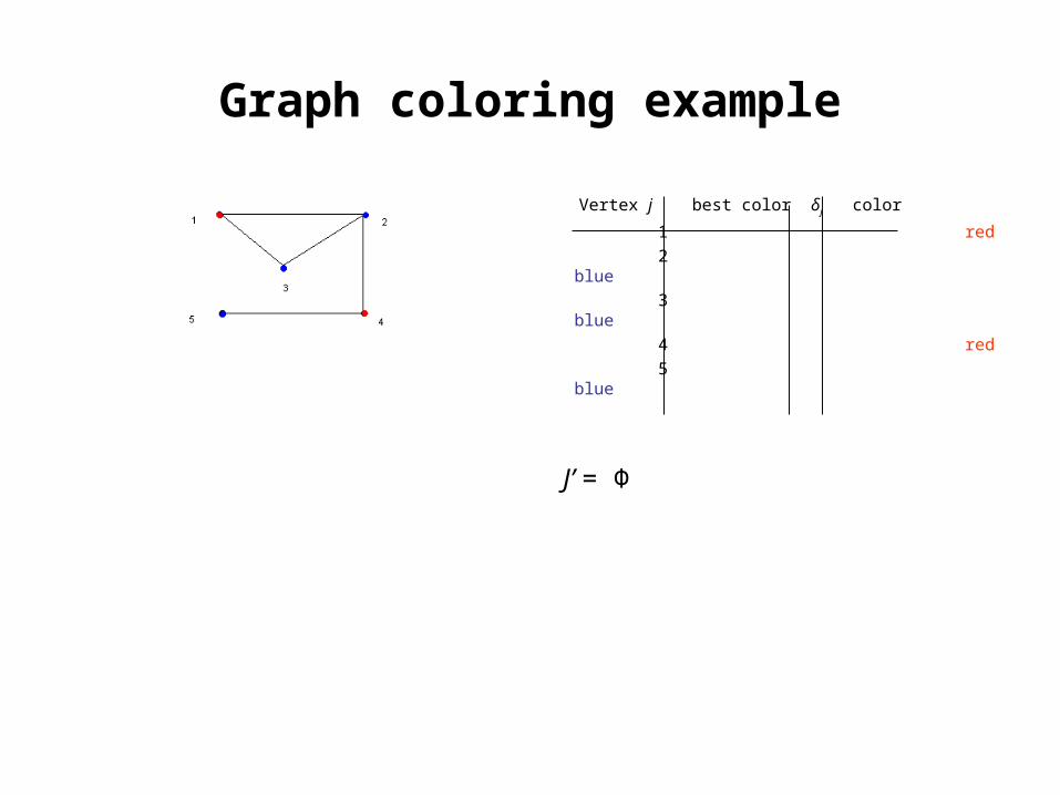
Vertex j best color δj color
1 red
2 blue
3 blue
4 red
5 blue
J’ = Φ
Neighborhood (Local) Search Techniques (NST)
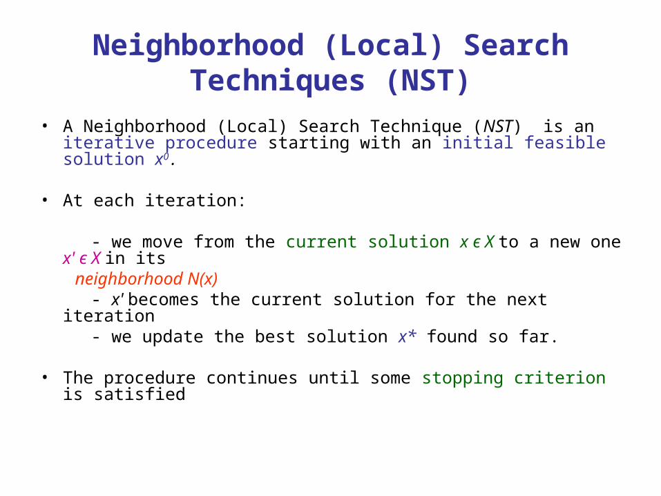
• A Neighborhood (Local) Search Technique (NST) is an iterative procedure starting with an initial feasible solution x0 .
• At each iteration:
- we move from the current solution x є X to a new one x' є X in its neighborhood N(x) - x' becomes the current solution for the next iteration - we update the best solution x* found so far.
• The procedure continues until some stopping criterion is satisfied
Neighborhood
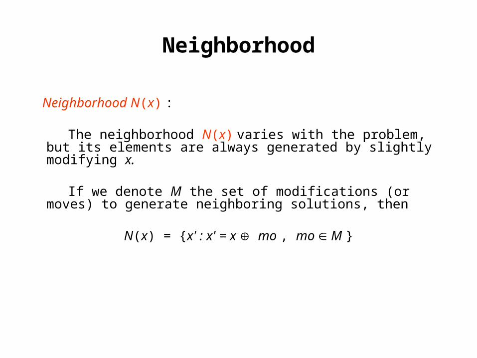
Neighborhood N(x) :
The neighborhood N(x) varies with the problem, but its elements are always generated by slightly modifying x.
If we denote M the set of modifications (or moves) to generate neighboring
solutions, then
N(x) = {x' : x' = x mo , mo M }
Neighborhood for assigment type problem
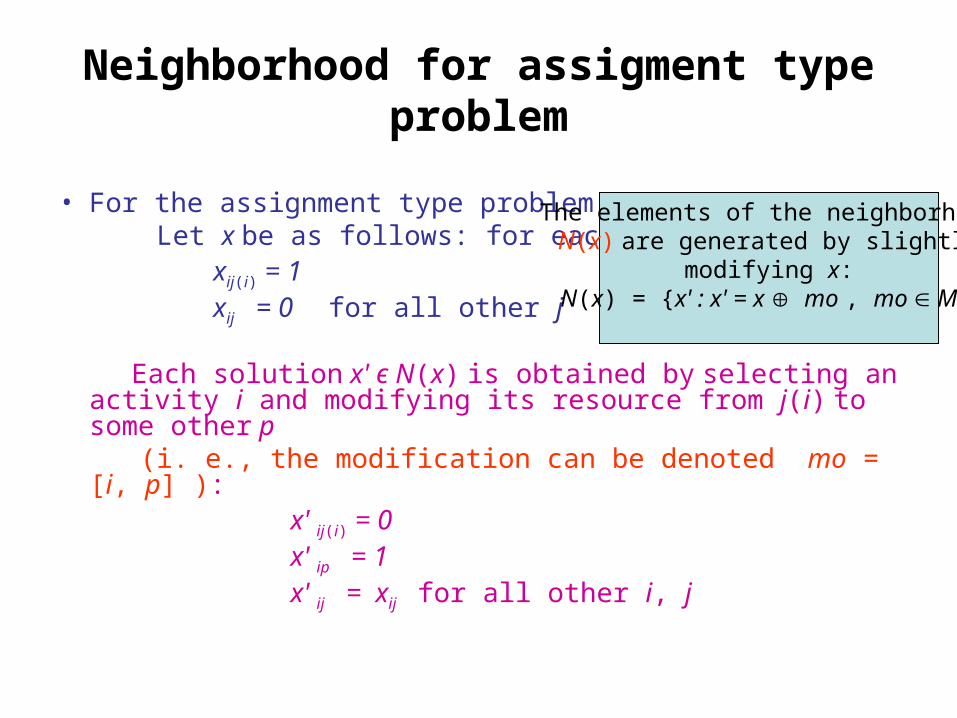
• For the assignment type problem: Let x be as follows: for each 1≤ i ≤ n, xij(i) = 1 xij = 0 for all other j
Each solution x' є N(x) is obtained by selecting an activity i and modifying its resource from j(i) to some other p
(i. e., the modification can be denoted mo = [i, p] ): x' ij(i) = 0 x' ip = 1 x' ij = xij for all other i, j
The elements of the neighborhood N(x) are generated by slightly
modifying x:N(x) = {x' : x' = x mo , mo M }
Neighborhood (Local) Search Techniques (NST)
• Descent method• Tabu Search• Simulated Annealing• Threshold Accepting
• Introduce these methods using pseudo-codes
Descent Method (D)
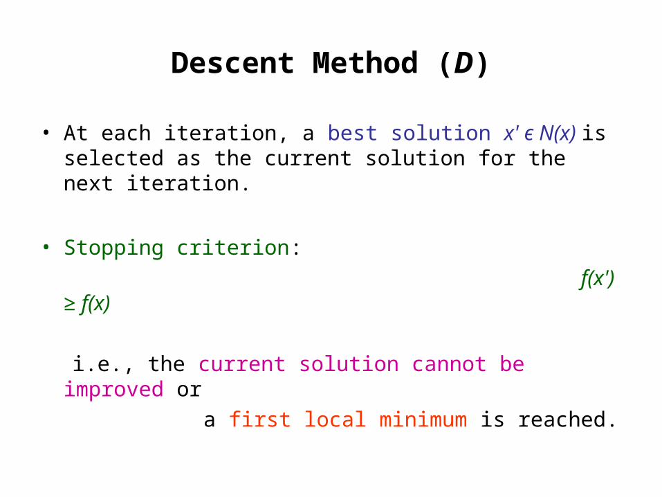
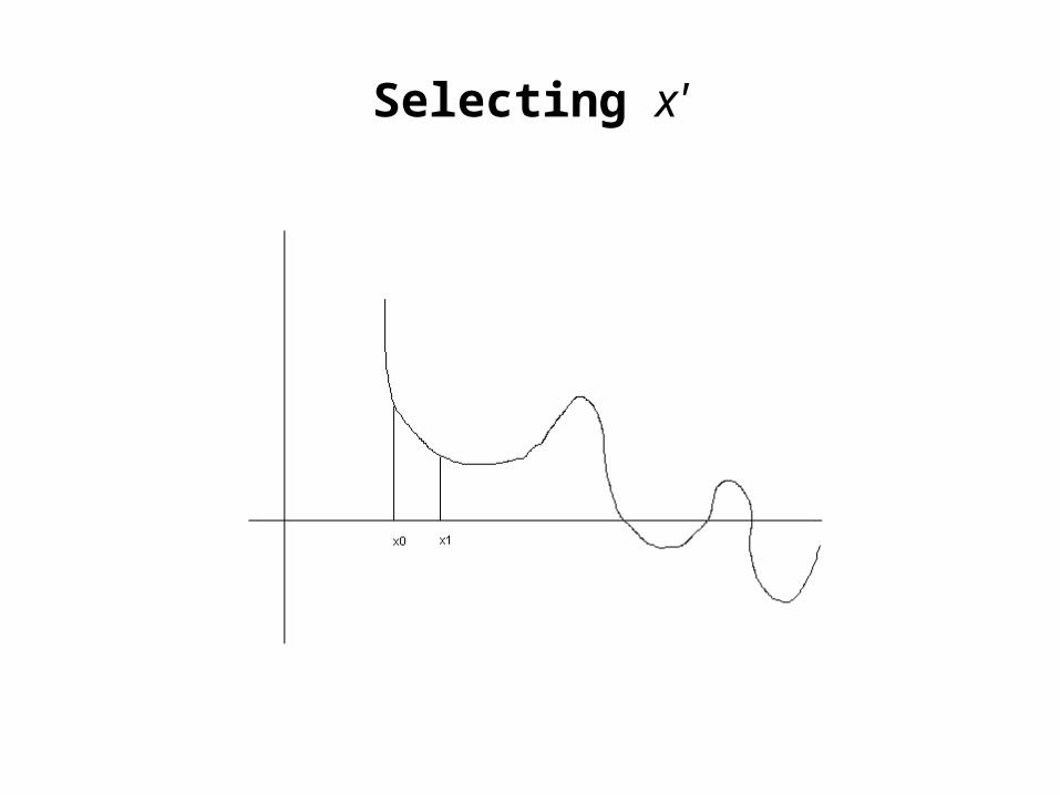
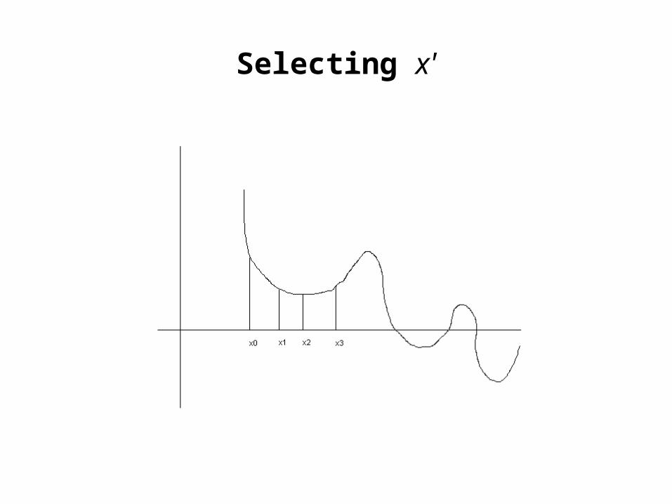
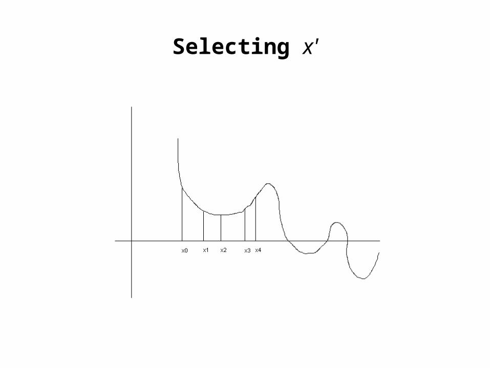
• At each iteration, a best solution x' є N(x) is selected as the current solution for the next iteration.
• Stopping criterion:
f(x') ≥ f(x)
i.e., the current solution cannot be improved or
a first local minimum is reached.

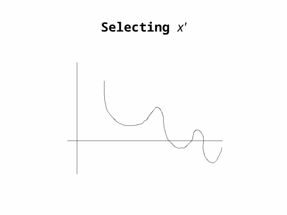
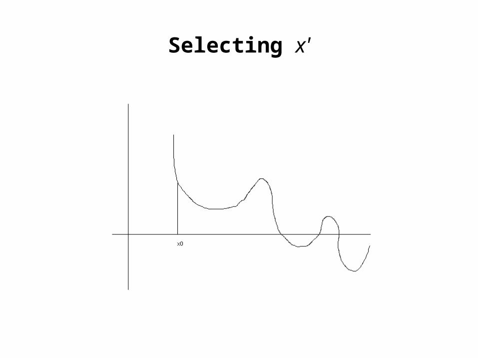
Selecting x'

Selecting x'

Selecting x'
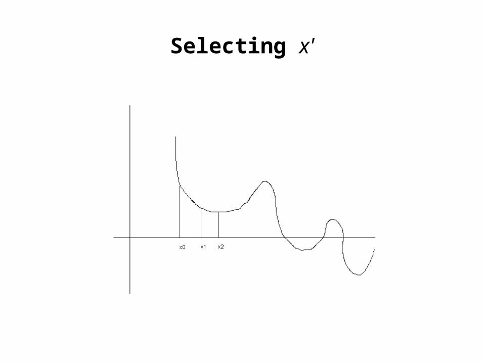
Selecting x'
Descent Method (D)
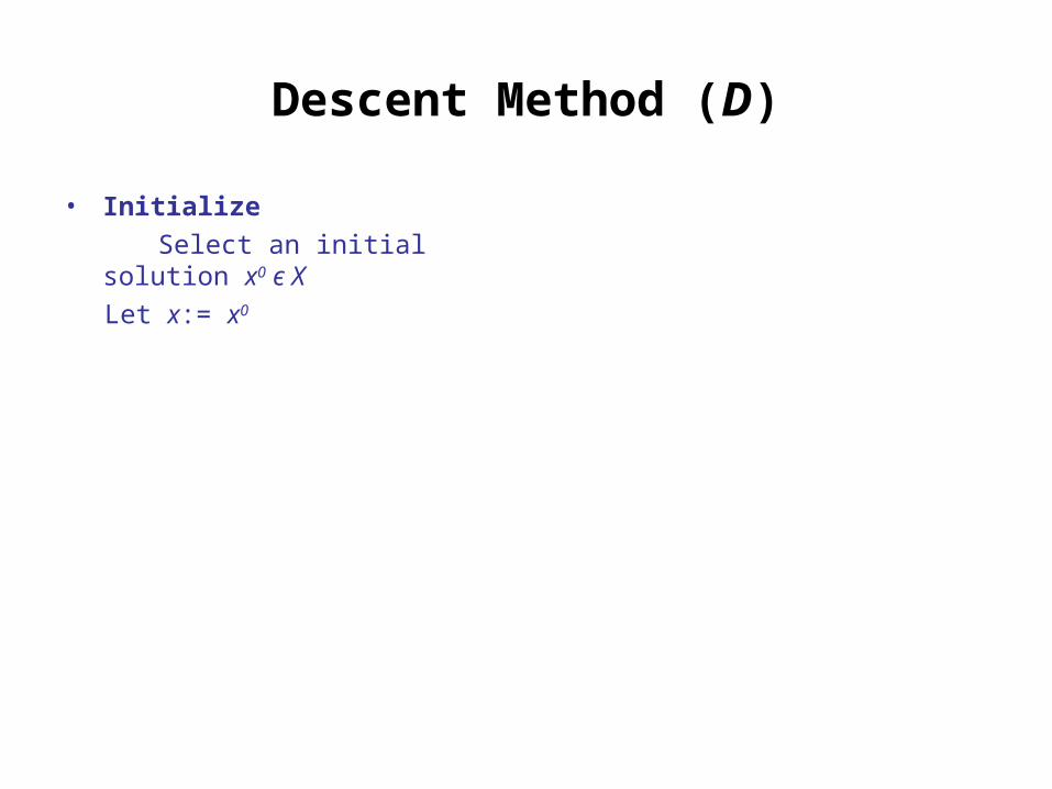
• Initialize
Select an initial solution x0 є X
Let x:= x0
Descent Method (D)
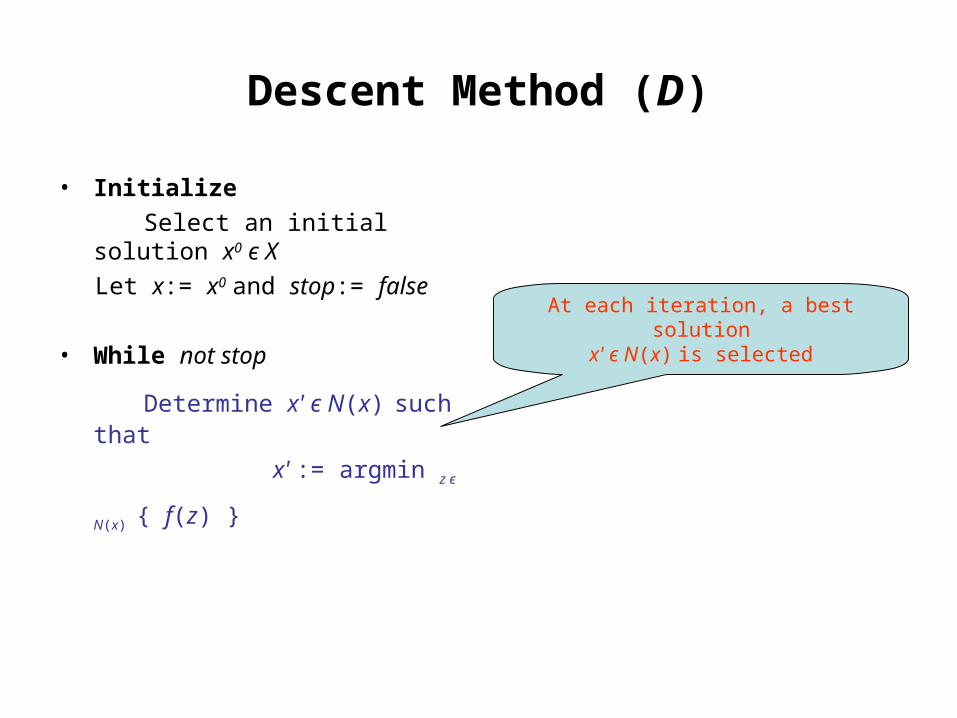
• Initialize
Select an initial solution x0 є X
Let x:= x0 and stop:= false
• While not stop
Determine x' є N(x) such that
x' := argmin z є N(x) { f(z) }
At each iteration, a best solutionx' є N(x) is selected
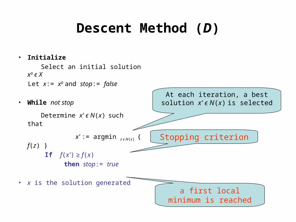
Descent Method (D)
• Initialize
Select an initial solution x0 є X
Let x:= x0 and stop:= false
• While not stop
Determine x' є N(x) such that
x' := argmin z є N(x) { f(z) }
If f(x') ≥ f(x)
then stop:= true
• x is the solution generated
Stopping criterion
At each iteration, a best solution x' є N(x) is selected
a first local minimum is reached
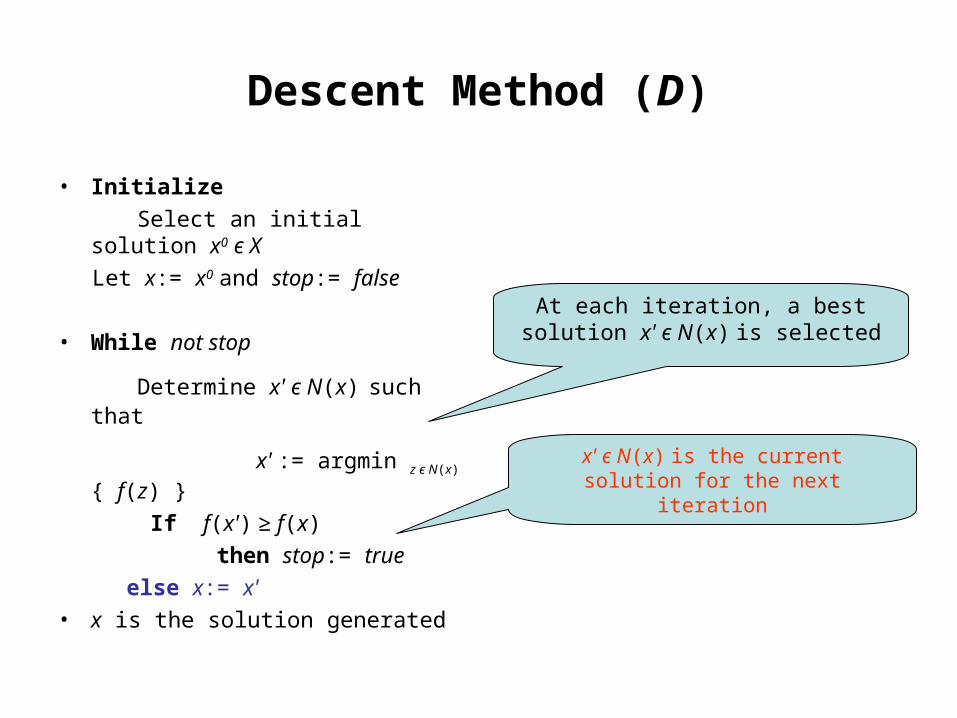
Descent Method (D)
• Initialize
Select an initial solution x0 є X
Let x:= x0 and stop:= false
• While not stop
Determine x' є N(x) such that
x' := argmin z є N(x) { f(z) }
If f(x') ≥ f(x)
then stop:= true
else x:= x'
• x is the solution generated
At each iteration, a best solution x' є N(x) is selected
x' є N(x) is the current solution for the next iteration
Graph coloring example
• Graph coloring problem : Graph G = (V,E). V = { i : 1≤ i ≤ n} ; E = {(i, l) : (i, l) edge of G}. Set of colors {j : 1≤ j ≤ m}
min f(x) = ∑ 1≤ j≤ m ∑ (i, l) є E xij xlj
Subject to ∑1≤ j≤ m xij = 1 1≤ i ≤ n
xij = 0 or 1 1≤ i ≤ n, 1≤ j ≤ m• To simplify notation, denote or encode a solution x as follows:
x => [j(1) , j(2) , …, j(i) , …, j(n)] where for each vertex i,
xij(i) = 1
xij = 0 for all other j
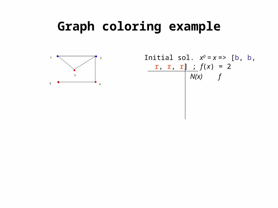
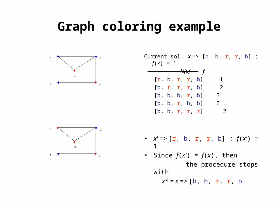
Graph coloring example
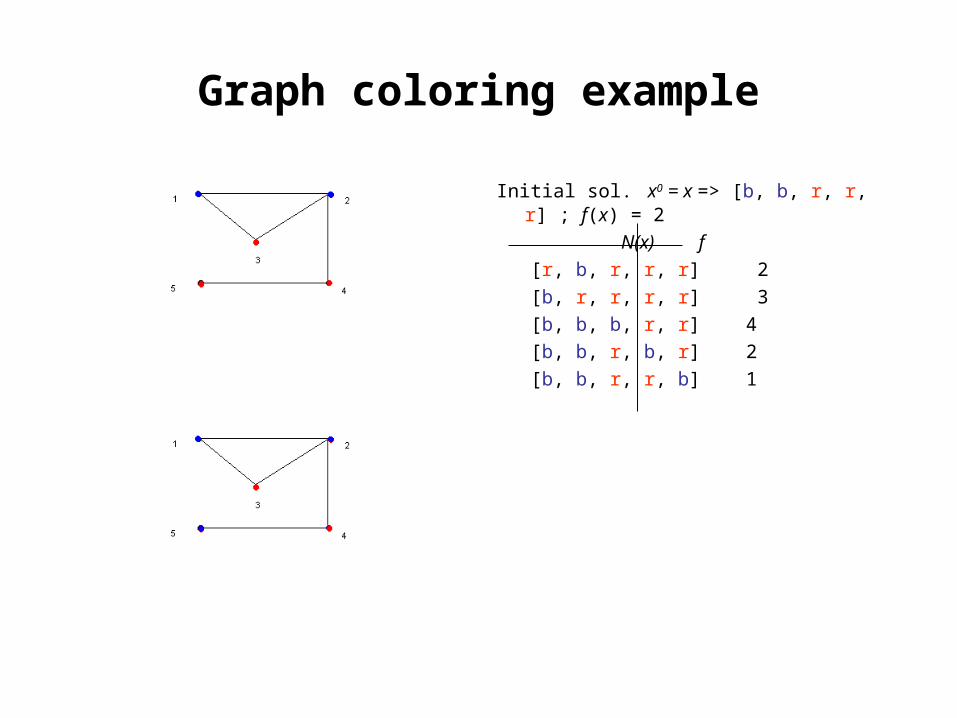
Initial sol. x0 = x => [b, b, r, r, r] ; f(x) = 2
N(x) f
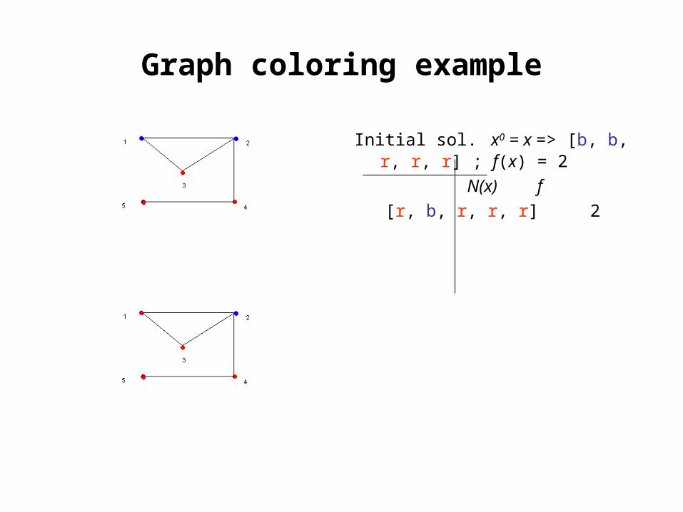
Graph coloring example
Initial sol. x0 = x => [b, b, r, r, r] ; f(x) = 2
N(x) f
[r, b, r, r, r] 2
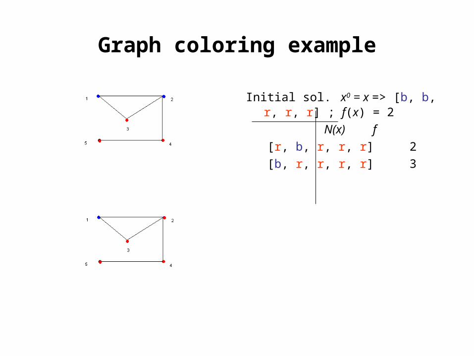
Graph coloring example
Initial sol. x0 = x => [b, b, r, r, r] ; f(x) = 2
N(x) f
[r, b, r, r, r] 2
[b, r, r, r, r] 3
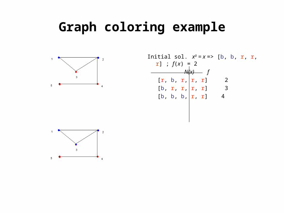
Graph coloring example
Initial sol. x0 = x => [b, b, r, r, r] ; f(x) = 2
N(x) f
[r, b, r, r, r] 2
[b, r, r, r, r] 3
[b, b, b, r, r] 4
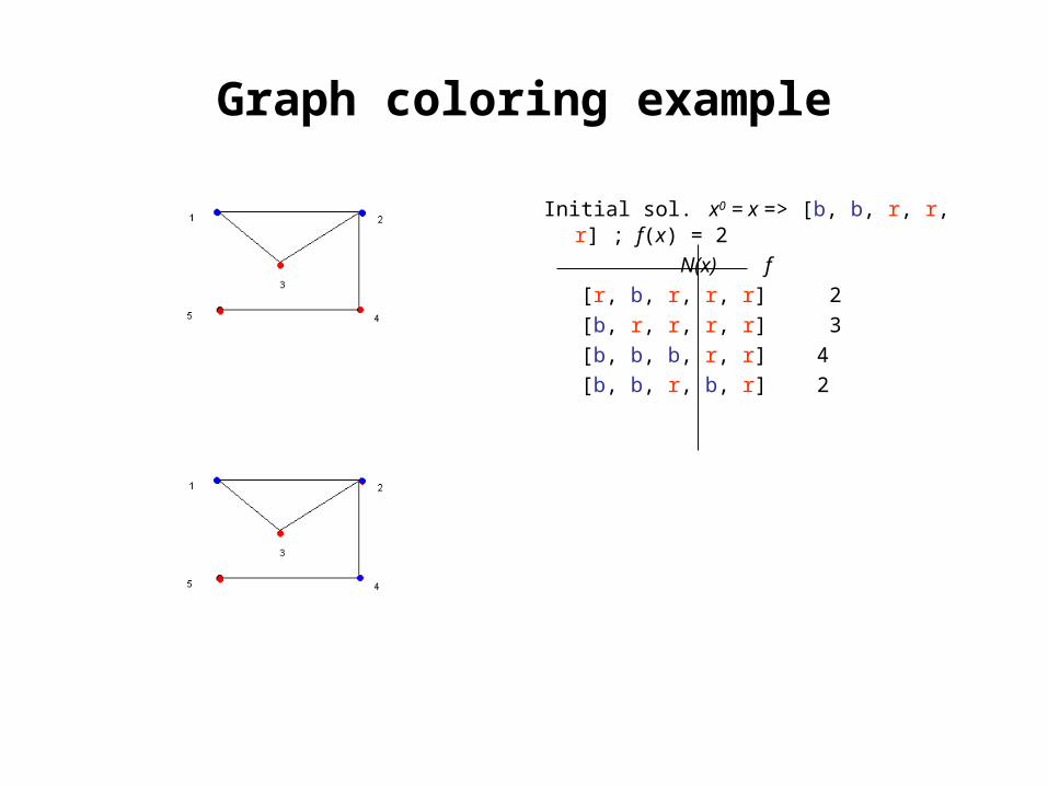
Graph coloring example
Initial sol. x0 = x => [b, b, r, r, r] ; f(x) = 2
N(x) f
[r, b, r, r, r] 2
[b, r, r, r, r] 3
[b, b, b, r, r] 4
[b, b, r, b, r] 2
Graph coloring example
Initial sol. x0 = x => [b, b, r, r, r] ; f(x) = 2
N(x) f
[r, b, r, r, r] 2
[b, r, r, r, r] 3
[b, b, b, r, r] 4
[b, b, r, b, r] 2
[b, b, r, r, b] 1
Graph coloring example
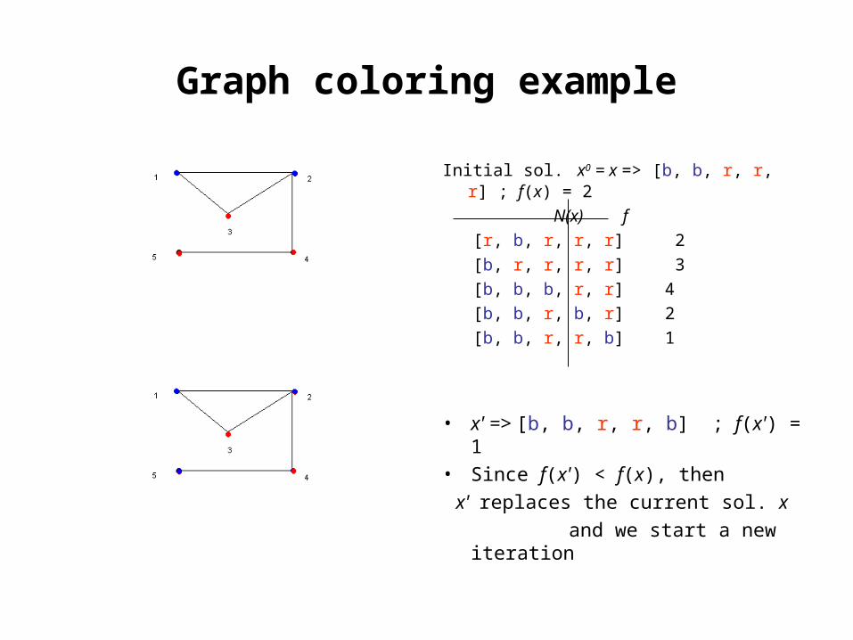
Initial sol. x0 = x => [b, b, r, r, r] ; f(x) = 2
N(x) f
[r, b, r, r, r] 2
[b, r, r, r, r] 3
[b, b, b, r, r] 4
[b, b, r, b, r] 2
[b, b, r, r, b] 1
• x' => [b, b, r, r, b] ; f(x') = 1
• Since f(x') < f(x), then
x' replaces the current sol. x
and we start a new iteration
Graph coloring example
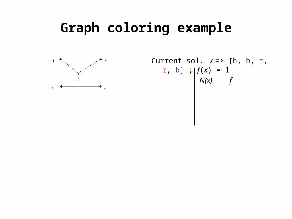
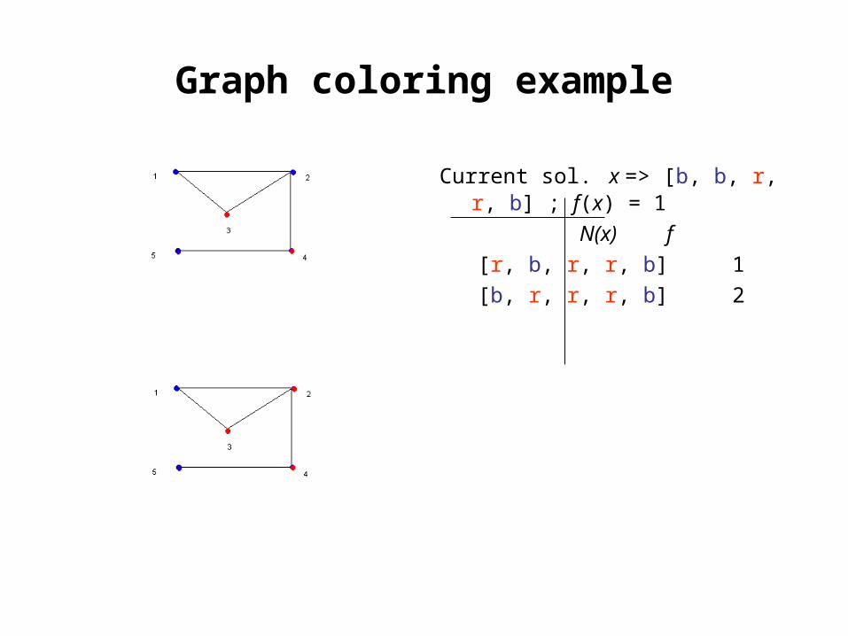
Current sol. x => [b, b, r, r, b] ; f(x) = 1
N(x) f
Graph coloring example
Current sol. x => [b, b, r, r, b] ; f(x) = 1
N(x) f
[r, b, r, r, b] 1
Graph coloring example
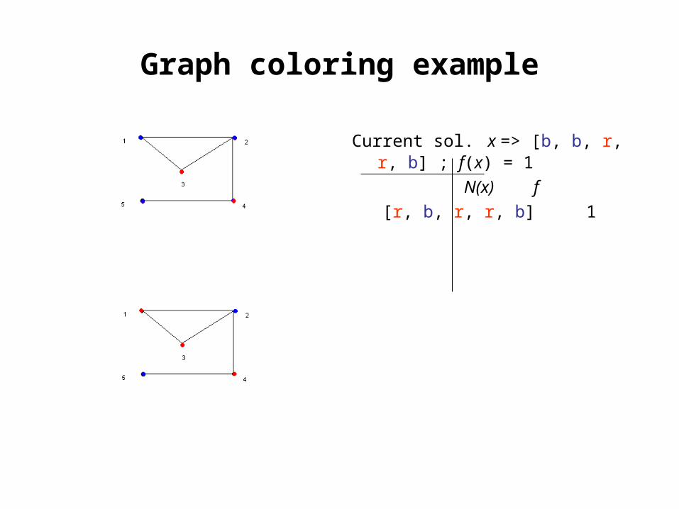
Current sol. x => [b, b, r, r, b] ; f(x) = 1
N(x) f
[r, b, r, r, b] 1
[b, r, r, r, b] 2
Graph coloring example
Current sol. x => [b, b, r, r, b] ; f(x) = 1
N(x) f
[r, b, r, r, b] 1
[b, r, r, r, b] 2
[b, b, b, r, b] 3
Graph coloring example
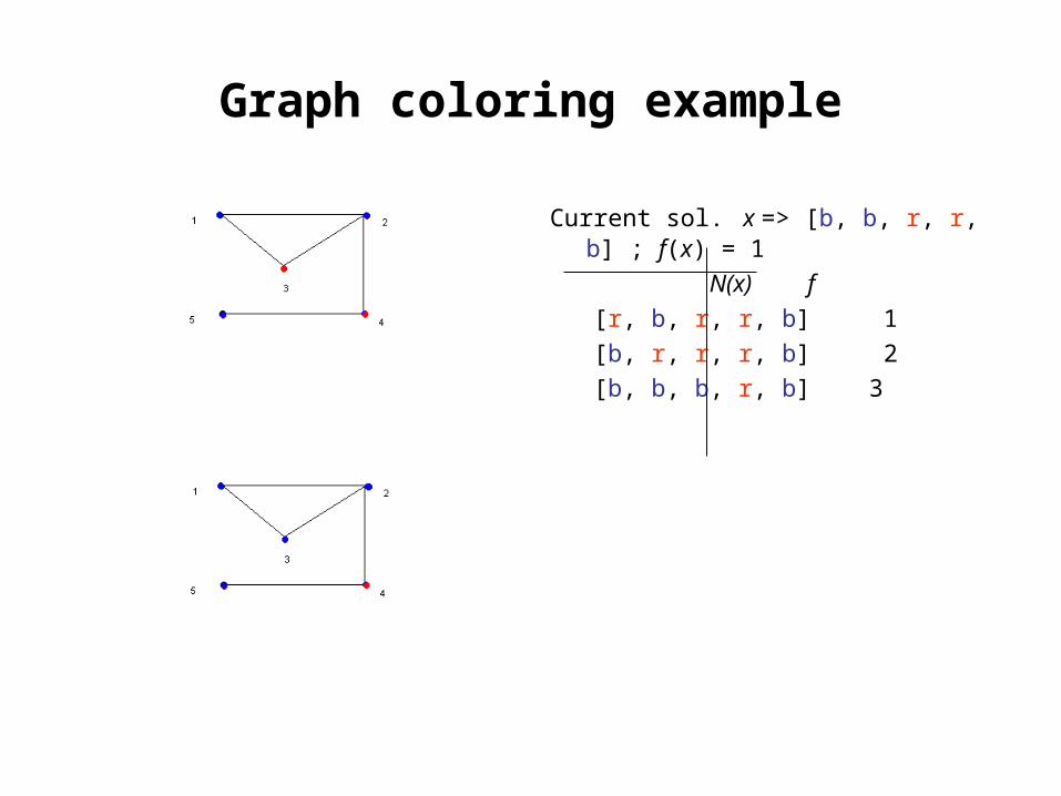
Current sol. x => [b, b, r, r, b] ; f(x) = 1
N(x) f
[r, b, r, r, b] 1
[b, r, r, r, b] 2
[b, b, b, r, b] 3
[b, b, r, b, b] 3
Graph coloring example
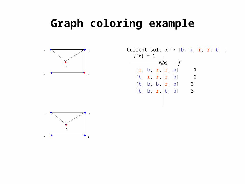
Current sol. x => [b, b, r, r, b] ; f(x) = 1
N(x) f
[r, b, r, r, b] 1
[b, r, r, r, b] 2
[b, b, b, r, b] 3
[b, b, r, b, b] 3
[b, b, r, r, r] 2
Graph coloring example
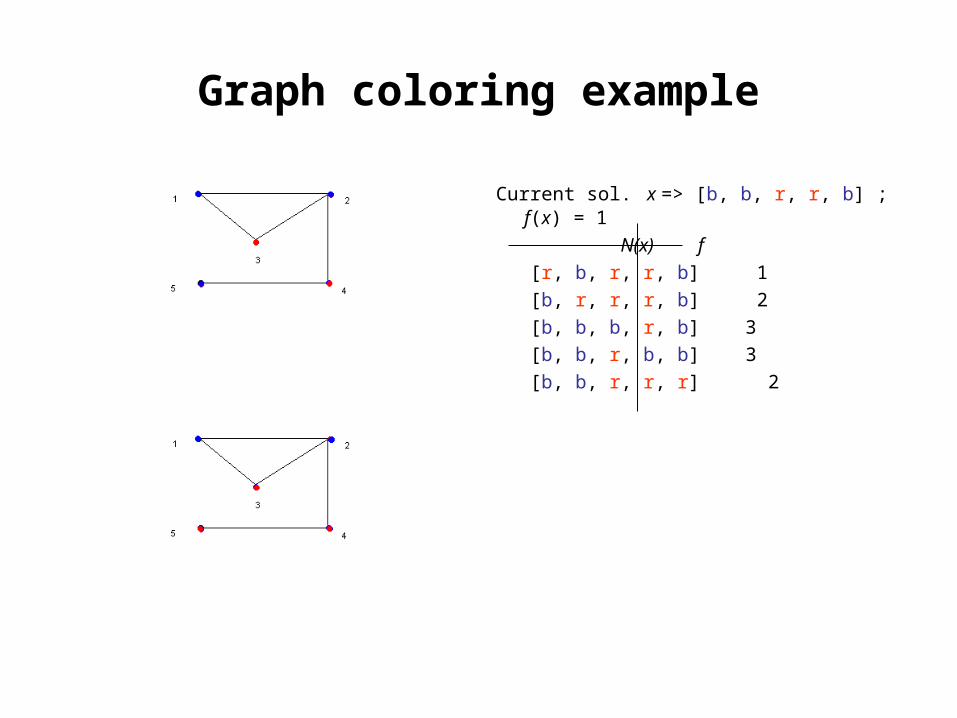
Current sol. x => [b, b, r, r, b] ; f(x) = 1
N(x) f
[r, b, r, r, b] 1
[b, r, r, r, b] 2
[b, b, b, r, b] 3
[b, b, r, b, b] 3
[b, b, r, r, r] 2
• x' => [r, b, r, r, b] ; f(x') = 1
• Since f(x') = f(x), then
the procedure stops with
x* = x => [b, b, r, r, b]
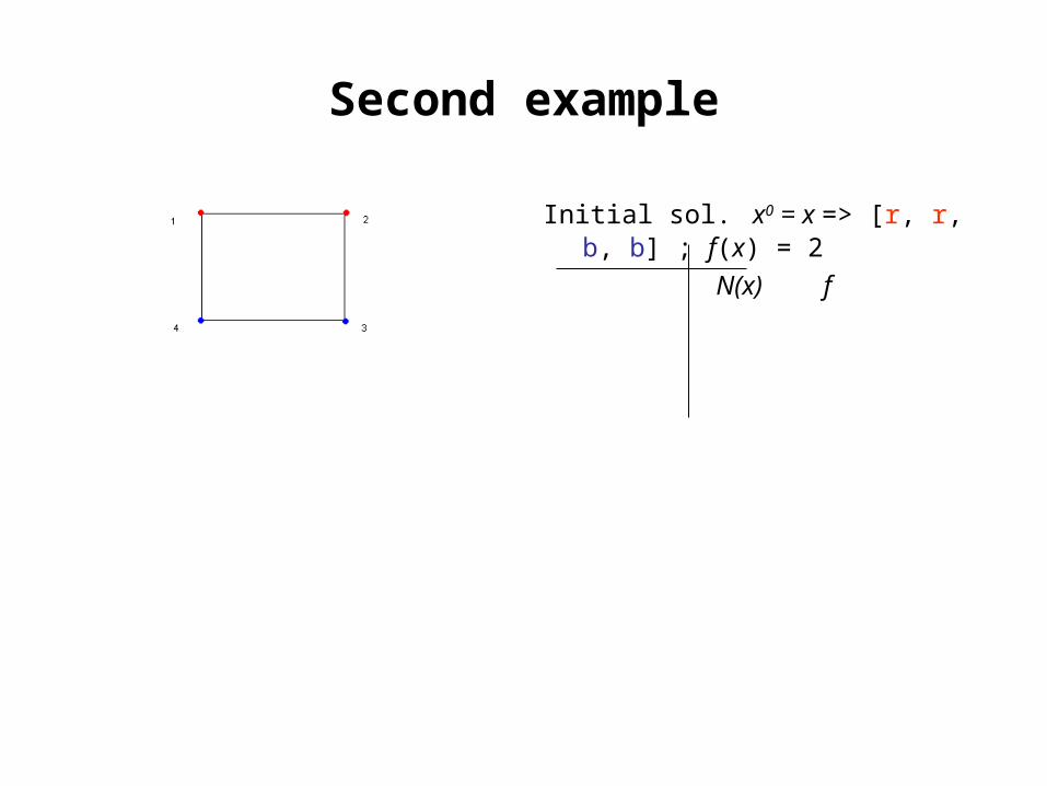
Second example
Initial sol. x0 = x => [r, r, b, b] ; f(x) = 2
N(x) f

Second example
Initial sol. x0 = x => [r, r, b, b] ; f(x) = 2
N(x) f
[b, r, b, b] 2

Second example
Initial sol. x0 = x => [r, r, b, b] ; f(x) = 2
N(x) f
[b, r, b, b] 2
[r, b, b, b] 2

Second example
Initial sol. x0 = x => [r, r, b, b] ; f(x) = 2
N(x) f
[b, r, b, b] 2
[r, b, b, b] 2
[r, r, r, b] 2
Second example
Initial sol. x0 = x => [r, r, b, b] ; f(x) = 2
N(x) f
[b, r, b, b] 2
[r, b, b, b] 2
[r, r, r, b] 2
[r, r, b, r] 2
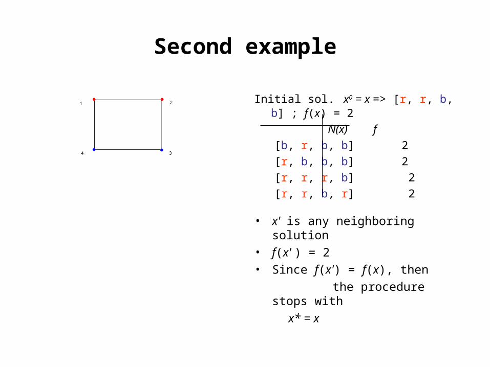
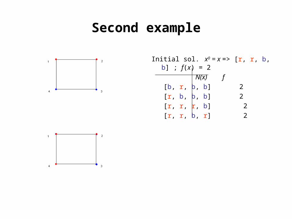
Second example
Initial sol. x0 = x => [r, r, b, b] ; f(x) = 2
N(x) f
[b, r, b, b] 2
[r, b, b, b] 2
[r, r, r, b] 2
[r, r, b, r] 2
• x' is any neighboring solution
• f(x' ) = 2
• Since f(x') = f(x), then
the procedure stops with
x* = x
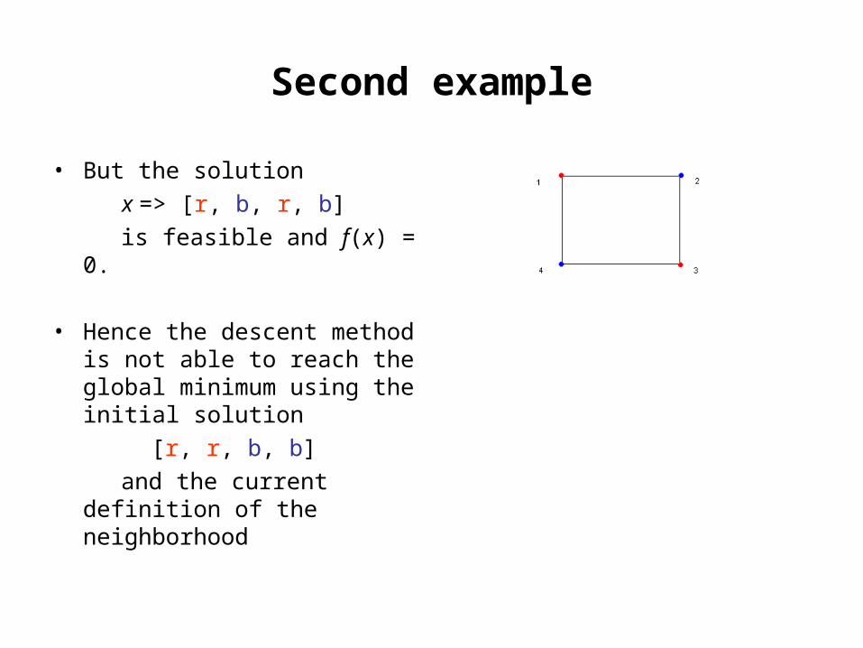
Second example
• But the solution
x => [r, b, r, b]
is feasible and f(x) = 0.
• Hence the descent method is not able to reach the global minimum using the initial solution
[r, r, b, b]
and the current definition of the neighborhood
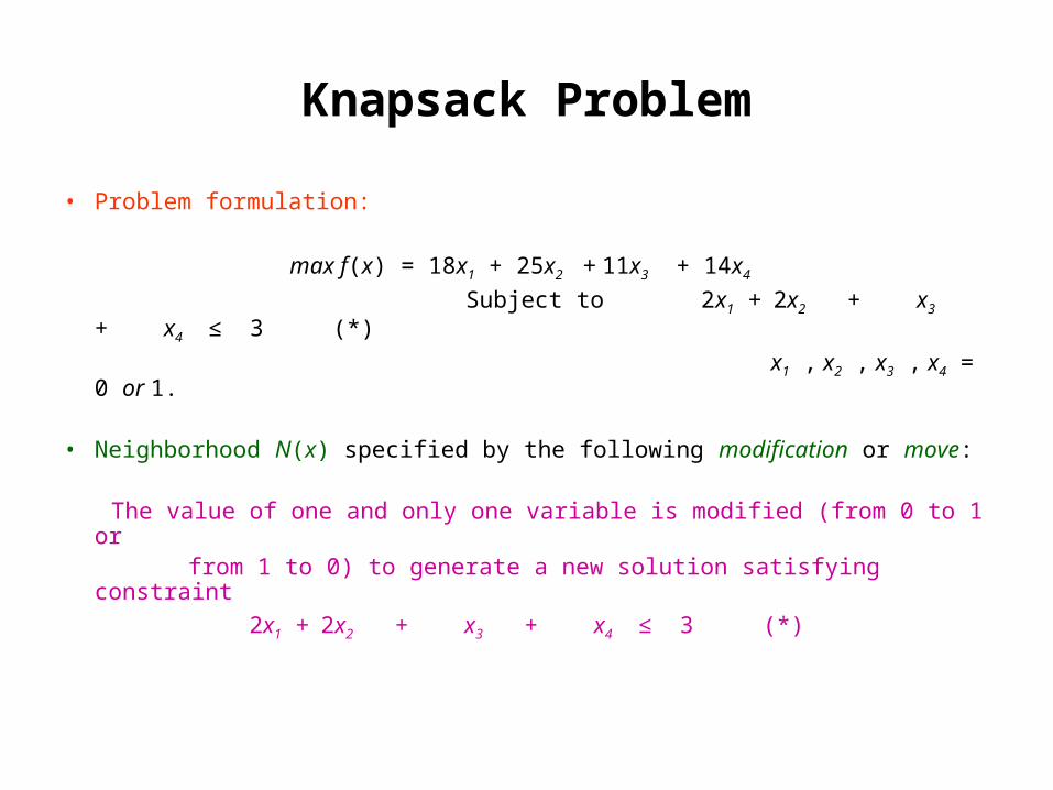
Knapsack Problem
• Problem formulation:
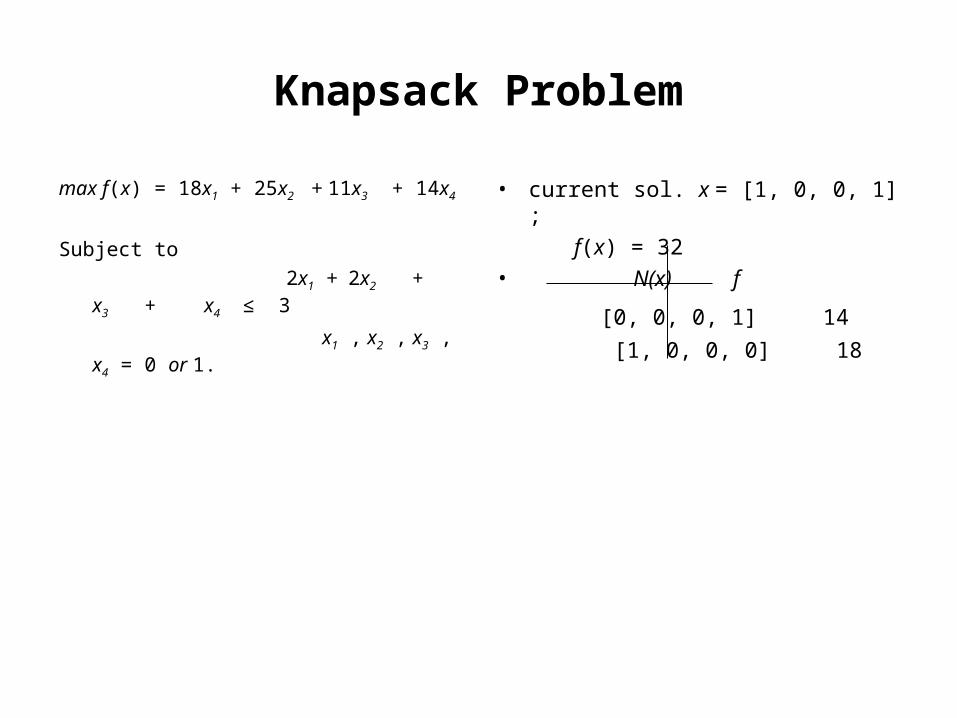
max f(x) = 18x1 + 25x2 + 11x3 + 14x4
Subject to 2x1 + 2x2 + x3 + x4 ≤ 3 (*)
x1 , x2 , x3 , x4 = 0 or 1.
• Neighborhood N(x) specified by the following modification or move:
The value of one and only one variable is modified (from 0 to 1 or from 1 to 0) to generate a new solution satisfying constraint
2x1 + 2x2 + x3 + x4 ≤ 3 (*)
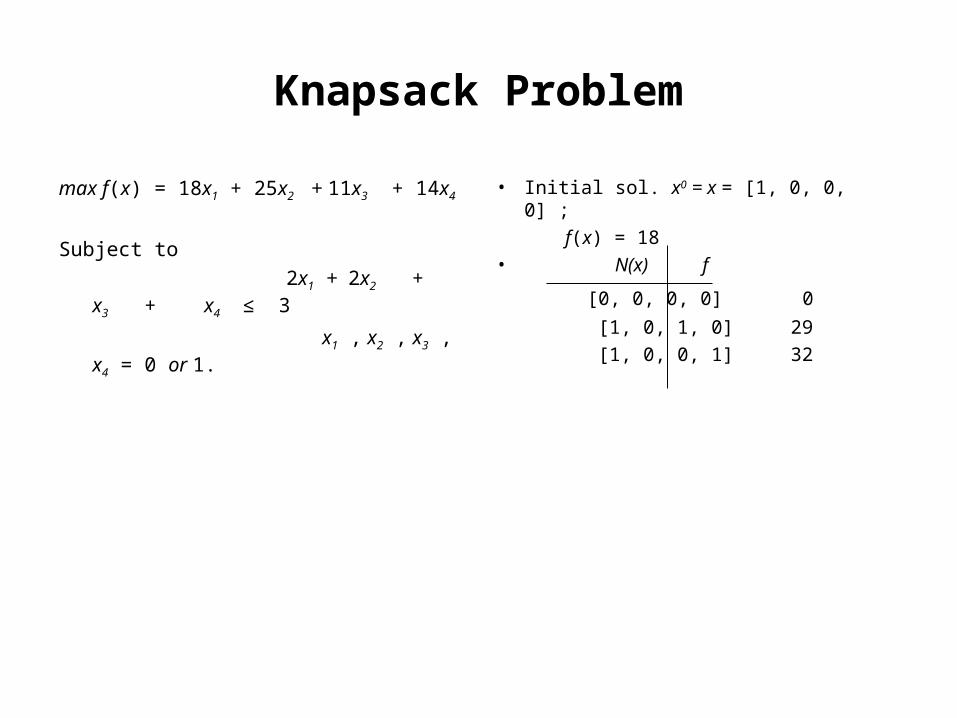
Knapsack Problem
max f(x) = 18x1 + 25x2 + 11x3 + 14x4
Subject to
2x1 + 2x2 + x3 + x4 ≤ 3
x1 , x2 , x3 , x4 = 0 or 1.
• Initial sol. x0 = x = [1, 0, 0, 0] ;
f(x) = 18• N(x) f
[0, 0, 0, 0] 0
[1, 0, 1, 0] 29
[1, 0, 0, 1] 32
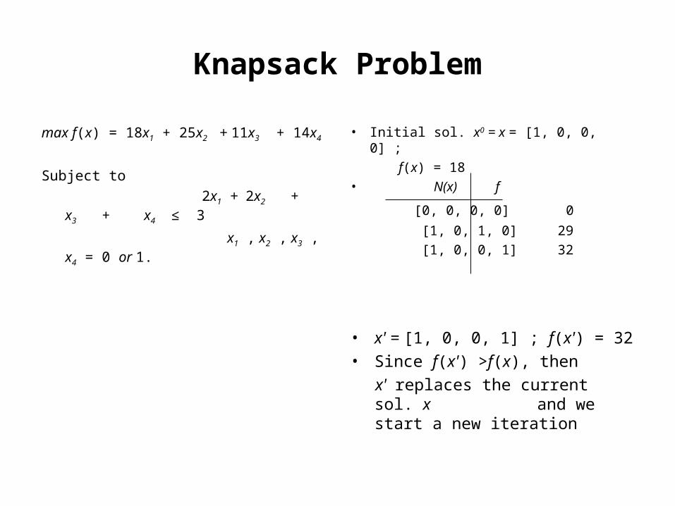
Knapsack Problem
max f(x) = 18x1 + 25x2 + 11x3 + 14x4
Subject to
2x1 + 2x2 + x3 + x4 ≤ 3
x1 , x2 , x3 , x4 = 0 or 1.
• Initial sol. x0 = x = [1, 0, 0, 0] ;
f(x) = 18• N(x) f
[0, 0, 0, 0] 0
[1, 0, 1, 0] 29
[1, 0, 0, 1] 32
• x' = [1, 0, 0, 1] ; f(x') = 32
• Since f(x') >f(x), then
x' replaces the current sol. x and we start a new iteration
Knapsack Problem
max f(x) = 18x1 + 25x2 + 11x3 + 14x4
Subject to
2x1 + 2x2 + x3 + x4 ≤ 3
x1 , x2 , x3 , x4 = 0 or 1.
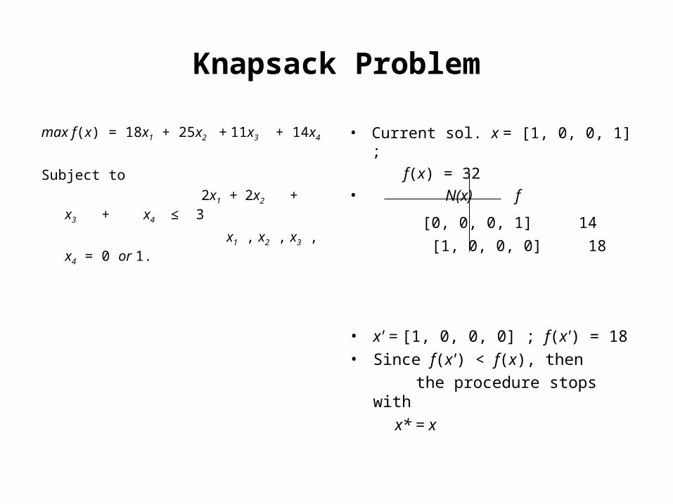
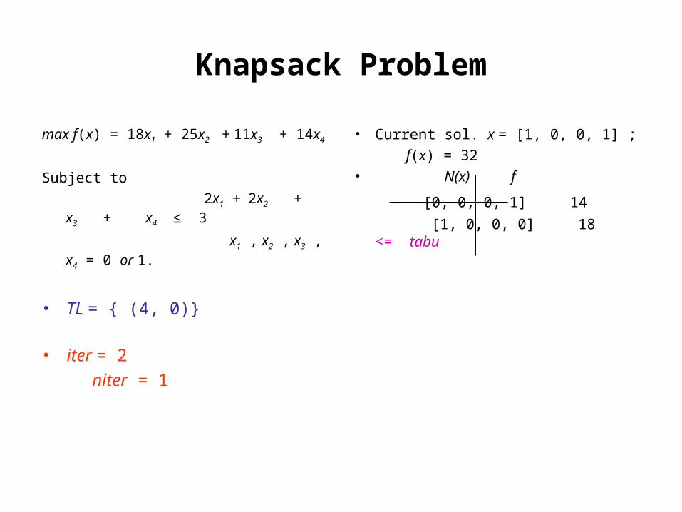
• current sol. x = [1, 0, 0, 1] ;
f(x) = 32
• N(x) f
[0, 0, 0, 1] 14
[1, 0, 0, 0] 18
Knapsack Problem
max f(x) = 18x1 + 25x2 + 11x3 + 14x4
Subject to
2x1 + 2x2 + x3 + x4 ≤ 3
x1 , x2 , x3 , x4 = 0 or 1.
• Current sol. x = [1, 0, 0, 1] ;
f(x) = 32
• N(x) f
[0, 0, 0, 1] 14
[1, 0, 0, 0] 18
• x' = [1, 0, 0, 0] ; f(x') = 18
• Since f(x') < f(x), then
the procedure stops with
x* = x

Tabu Search
• Tabu Search is an iterative neighborhood or local search technique
• At each iteration we move from a current solution x to a new solution x' in a neigborhood of x denoted N(x),
• until we reach some solution x* acceptable according to some criterion
Selecting x'
Selecting x'
Selecting x'

Selecting x'
Selecting x'
Selecting x'

Selecting x'

Tabu Search (TS)

Tabu Search (TS)
• Initialize Select an initial solution x0 є X
Let x:= x0
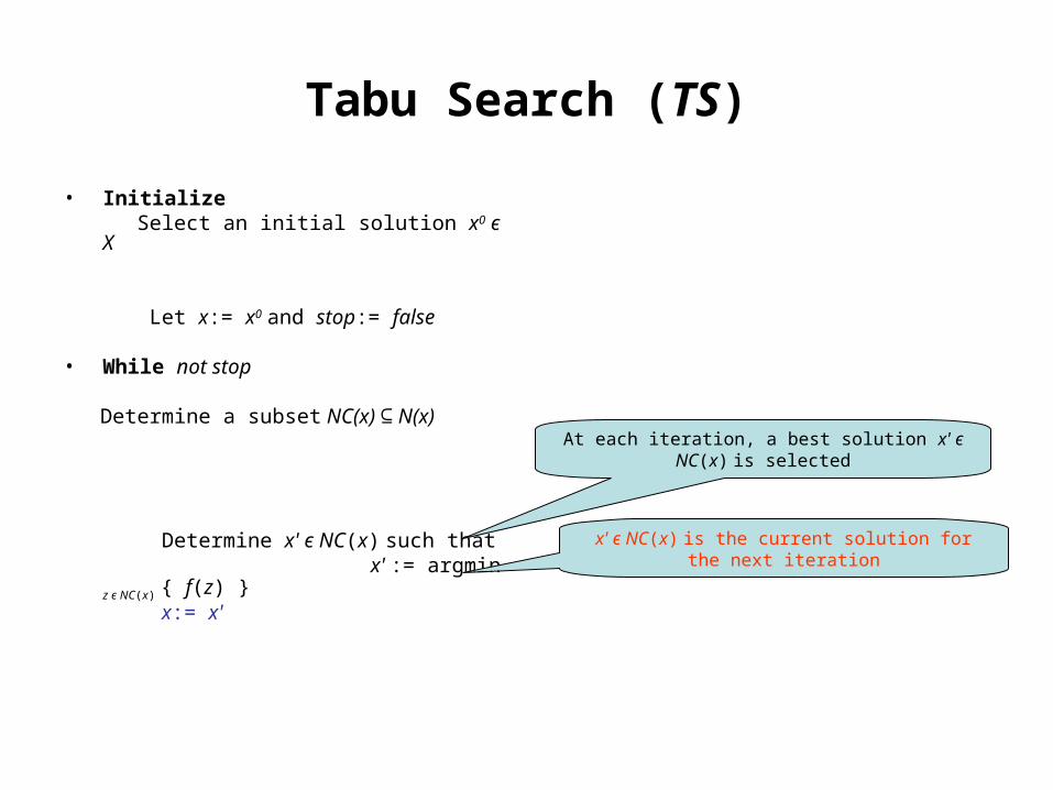
Tabu Search (TS)
• Initialize Select an initial solution x0 є X
Let x:= x0 and stop:= false
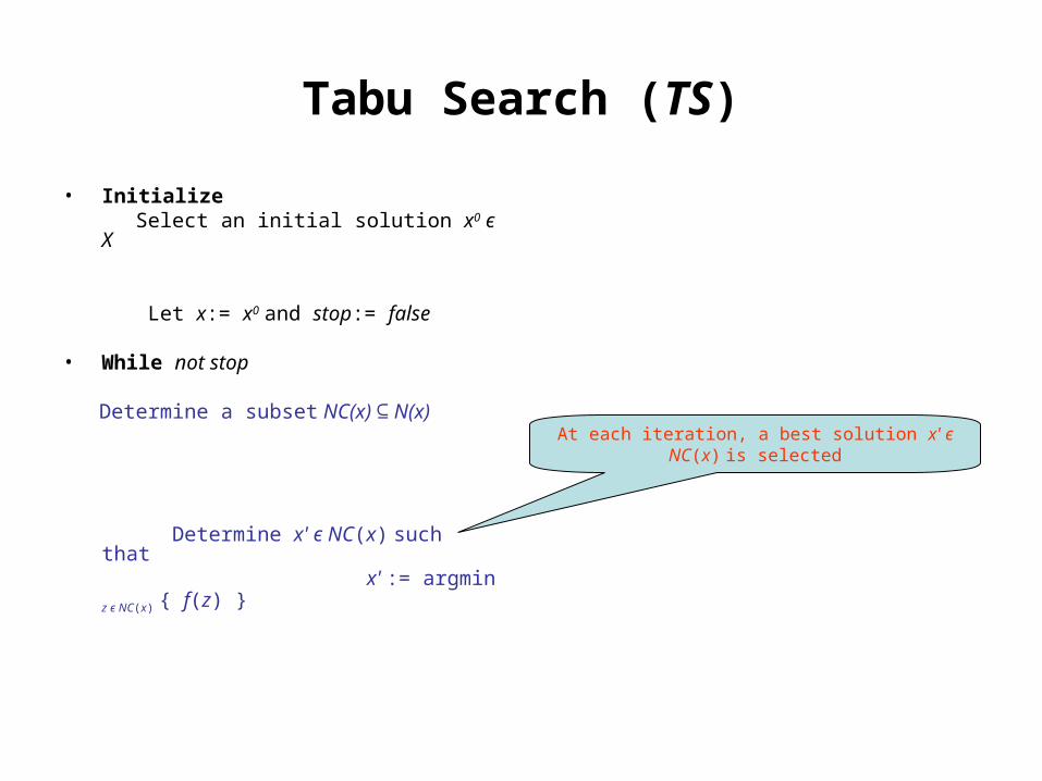
• While not stop Determine a subset NC(x) N(x) ⊆
Determine x' є NC(x) such that x' := argmin z є NC(x) { f(z) }
At each iteration, a best solution x' є NC(x) is selected
Tabu Search (TS)
• Initialize Select an initial solution x0 є X
Let x:= x0 and stop:= false
• While not stop Determine a subset NC(x) N(x) ⊆
Determine x' є NC(x) such that x' := argmin z є NC(x) { f(z) } x:= x'
At each iteration, a best solution x' є NC(x) is selected
x' є NC(x) is the current solution for the next iteration
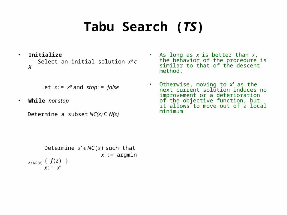
Tabu Search (TS)
• Initialize Select an initial solution x0 є X
Let x:= x0 and stop:= false
• While not stop Determine a subset NC(x) N(x)⊆
Determine x' є NC(x) such that x' := argmin z є NC(x) { f(z) } x:= x'
• As long as x' is better than x, the behavior of the procedure is similar to that of the descent method.
• Otherwise, moving to x' as the next current solution induces no improvement or a deterioration of the objective function, but it allows to move out of a local minimum
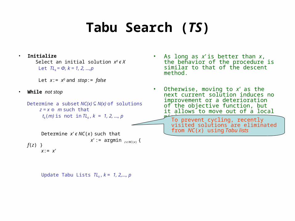
Tabu Search (TS)
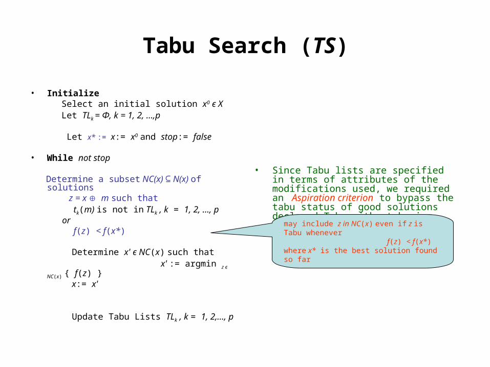
• Initialize Select an initial solution x0 є X Let TLk = Φ, k = 1, 2, …,p
Let x:= x0 and stop:= false
• While not stop Determine a subset NC(x) N(x) ⊆ of solutions z = x m such that tk(m) is not in TLk , k = 1, 2, …, p
Determine x' є NC(x) such that x' := argmin z є NC(x) { f(z) } x:= x'
Update Tabu Lists TLk , k = 1, 2,…, p
• As long as x' is better than x, the behavior of the procedure is similar to that of the descent method.
• Otherwise, moving to x' as the next current solution induces no improvement or a deterioration of the objective function, but it allows to move out of a local minimum
To prevent cycling, recently visited solutions are eliminated from NC(x) using Tabu lists
Tabu Lists (TL)
• Short term Tabu lists TLk are used to remember attributes or characteristics of the modification used to generate the new current solution
• A Tabu List often used for the assignment type problem is the following:
If the new current solution x' is generated from x by modifying the resource of i from j(i) to p, then the pair (i, j(i)) is introduced in the Tabu list TL
If the pair (i, j) is in TL, then any solution where resource j is to be assigned to i is declared Tabu
• The Tabu lists are cyclic in order for an attribute to remain Tabu for a fixed number nk of iterations

Tabu Search (TS)
• Initialize Select an initial solution x0 є X Let TLk = Φ, k = 1, 2, …,p
Let x:= x0 and stop:= false
• While not stop Determine a subset NC(x) N(x) ⊆ of solutions z = x m such that tk(m) is not in TLk , k = 1, 2, …, p
Determine x' є NC(x) such that x' := argmin z є NC(x) { f(z) } x:= x'
Update Tabu Lists TLk , k = 1, 2,…, p
• As long as x' is better than x, the behavior of the procedure is similar to that of the descent method.
• Otherwise, moving to x' as the next current solution induces no improvement or a deterioration of the objective function, but it allows to move out of a local minimum
To prevent cycling, recently visited solutions are eliminated from NC(x) using Tabu lists
Tabu Search (TS)
• Initialize Select an initial solution x0 є X Let TLk = Φ, k = 1, 2, …,p
Let x* := x:= x0 and stop:= false
• While not stop Determine a subset NC(x) N(x) ⊆ of solutions z = x m such that tk(m) is not in TLk , k = 1, 2, …, p or f(z) < f(x*)
Determine x' є NC(x) such that x' := argmin z є NC(x) { f(z) } x:= x' Update Tabu Lists TLk , k = 1, 2,…, p
• Since Tabu lists are specified in terms of attributes of the modifications used, we required an Aspiration criterion to bypass the tabu status of good solutions declared Tabu without having been visited recently
may include z in NC(x) even if z is Tabu whenever f(z) < f(x*) where x* is the best solution found so far

Tabu Search (TS)
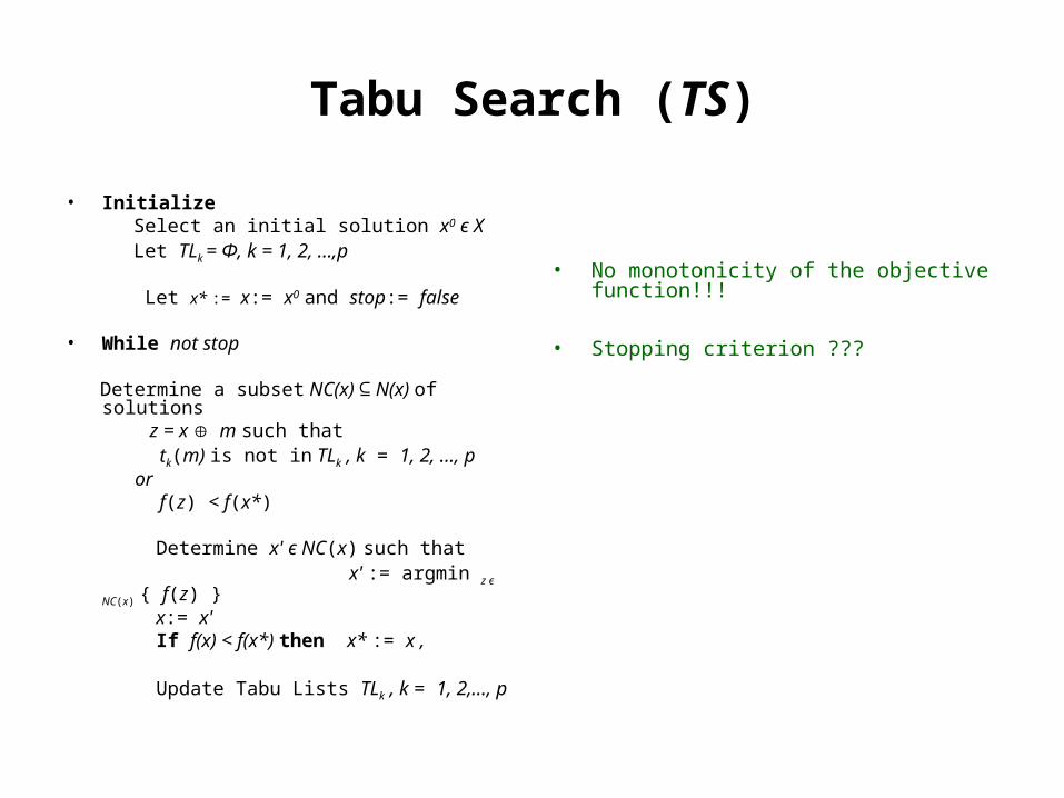
• Initialize Select an initial solution x0 є X Let TLk = Φ, k = 1, 2, …,p
Let x* := x:= x0 and stop:= false
• While not stop Determine a subset NC(x) N(x) ⊆ of solutions z = x m such that tk(m) is not in TLk , k = 1, 2, …, p or f(z) < f(x*)
Determine x' є NC(x) such that x' := argmin z є NC(x) { f(z) } x:= x' If f(x) < f(x*) then x* := x , Update Tabu Lists TLk , k = 1, 2,…, p
Update x* the best solution found so far
Tabu Search (TS)
• Initialize Select an initial solution x0 є X Let TLk = Φ, k = 1, 2, …,p
Let x* := x:= x0 and stop:= false
• While not stop Determine a subset NC(x) N(x) ⊆ of solutions z = x m such that tk(m) is not in TLk , k = 1, 2, …, p or f(z) < f(x*)
Determine x' є NC(x) such that x' := argmin z є NC(x) { f(z) } x:= x' If f(x) < f(x*) then x* := x ,
Update Tabu Lists TLk , k = 1, 2,…, p
• No monotonicity of the objective function!!!
• Stopping criterion ???

Tabu Search (TS)
• Initialize Select an initial solution x0 є X Let TLk = Φ, k = 1, 2, …,p Let iter := niter := 0 Let x* := x:= x0 and stop:= false
• While not stop iter := iter + 1 ; niter := niter + 1 Determine a subset NC(x) N(x) ⊆ of solutions z = x m such that tk(m) is not in TLk , k = 1, 2, …, p or f(z) < f(x*) Determine x' є NC(x) such that x' := argmin z є NC(x) { f(z) } x:= x' If f(x) < f(x*) then x* := x , and niter := 0 If iter = itermax or niter = nitermax then stop := true Update Tabu Lists TLk , k = 1, 2,…, p• x* is the best solution generated
Stopping criteria: - maximum number of iterations - maximum number of successive iterations where f(x*) does not improve
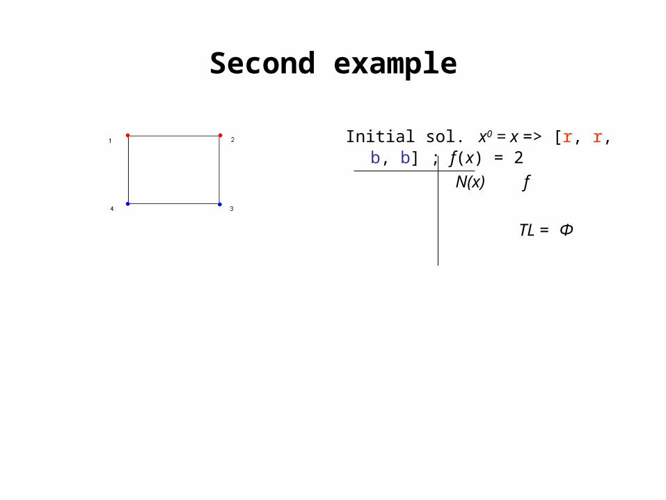
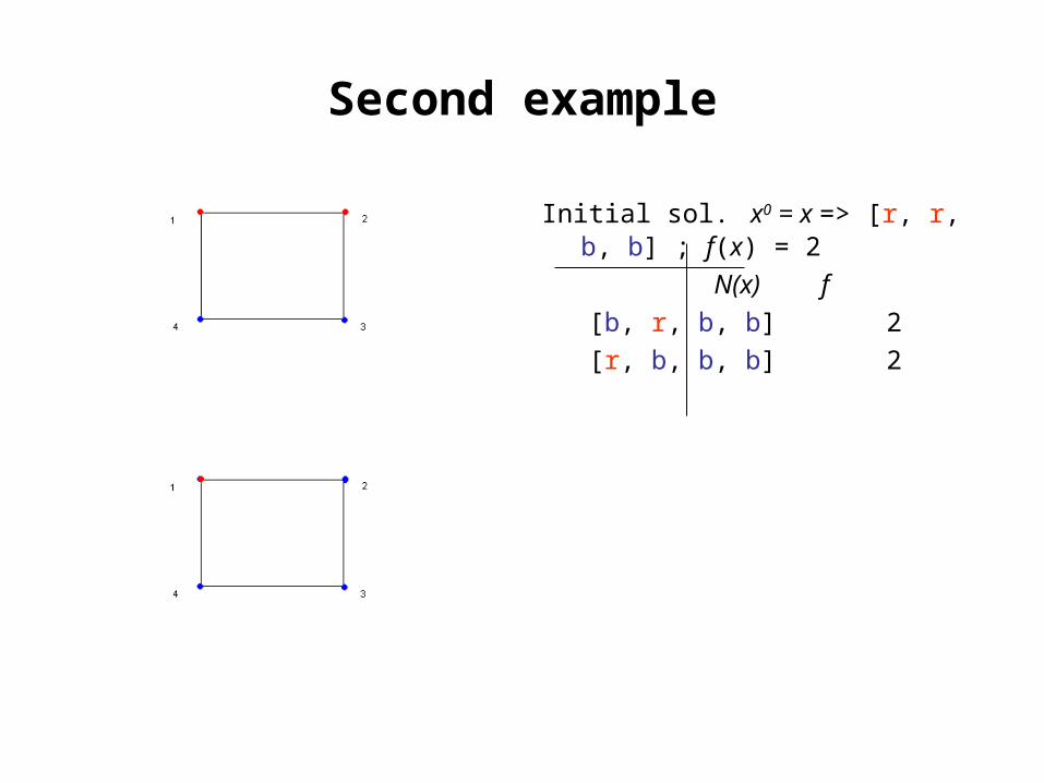
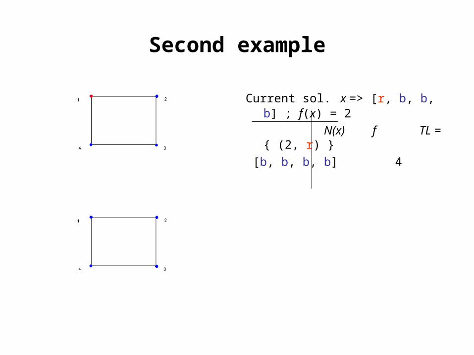
Second example
Initial sol. x0 = x => [r, r, b, b] ; f(x) = 2
N(x) f
TL = Φ
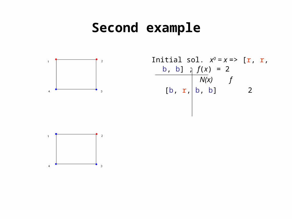
Second example
Initial sol. x0 = x => [r, r, b, b] ; f(x) = 2
N(x) f
[b, r, b, b] 2
Second example
Initial sol. x0 = x => [r, r, b, b] ; f(x) = 2
N(x) f
[b, r, b, b] 2
[r, b, b, b] 2
Second example
Initial sol. x0 = x => [r, r, b, b] ; f(x) = 2
N(x) f
[b, r, b, b] 2
[r, b, b, b] 2
[r, r, r, b] 2

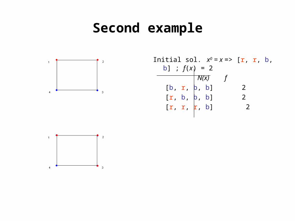
Second example
Initial sol. x0 = x => [r, r, b, b] ; f(x) = 2
N(x) f
[b, r, b, b] 2
[r, b, b, b] 2
[r, r, r, b] 2
[r, r, b, r] 2
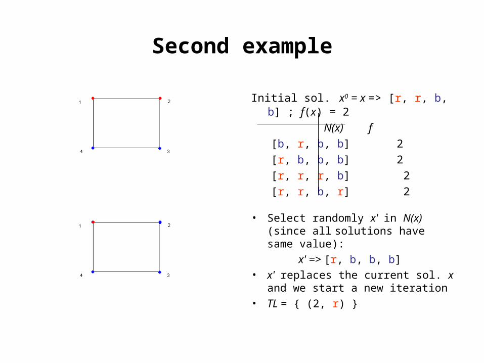
Second example
Initial sol. x0 = x => [r, r, b, b] ; f(x) = 2
N(x) f
[b, r, b, b] 2
[r, b, b, b] 2
[r, r, r, b] 2
[r, r, b, r] 2
• Select randomly x' in N(x) (since all solutions have same value):
x' => [r, b, b, b]
• x' replaces the current sol. x and we start a new iteration
• TL = { (2, r) }
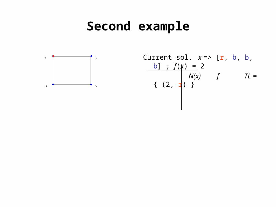
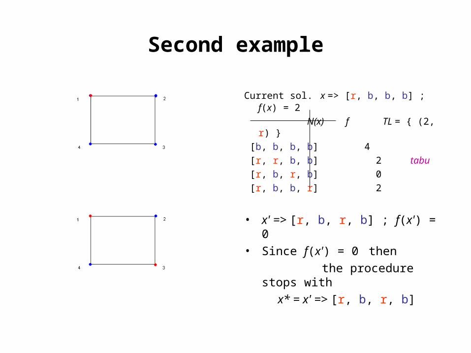
Second example
Current sol. x => [r, b, b, b] ; f(x) = 2
N(x) f TL = { (2, r) }
Second example
Current sol. x => [r, b, b, b] ; f(x) = 2
N(x) f TL = { (2, r) }
[b, b, b, b] 4
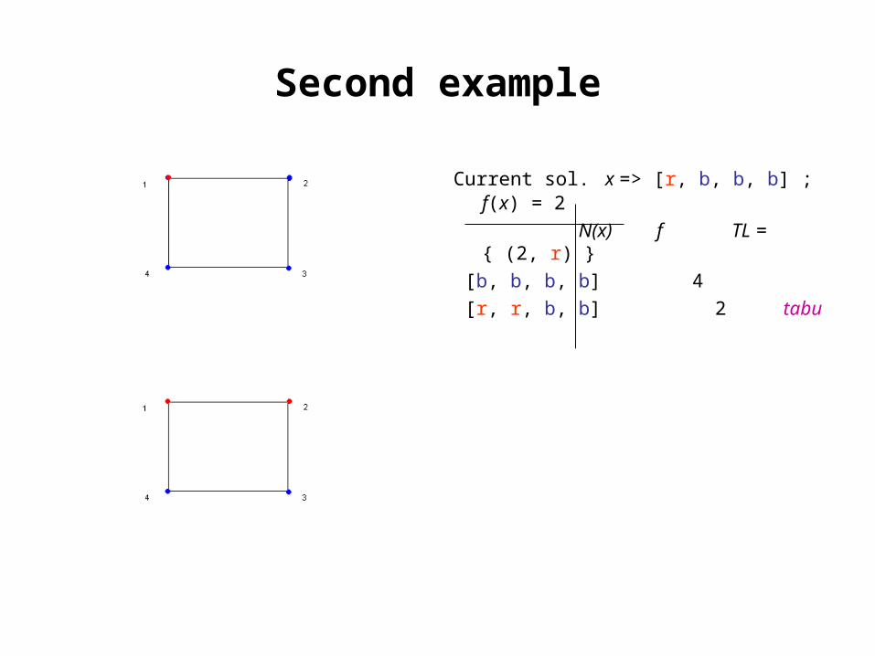
Second example
Current sol. x => [r, b, b, b] ; f(x) = 2
N(x) f TL = { (2, r) }
[b, b, b, b] 4
[r, r, b, b] 2 tabu
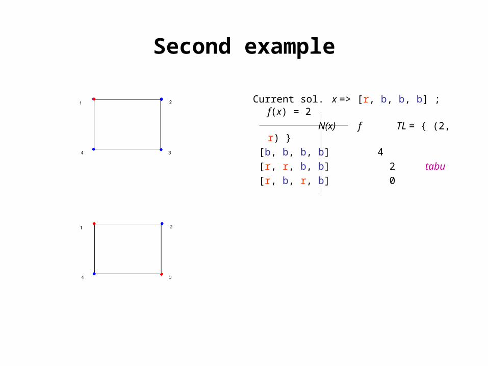
Second example
Current sol. x => [r, b, b, b] ; f(x) = 2
N(x) f TL = { (2, r) }
[b, b, b, b] 4
[r, r, b, b] 2 tabu
[r, b, r, b] 0
Second example
Current sol. x => [r, b, b, b] ; f(x) = 2
N(x) f TL = { (2, r) }
[b, b, b, b] 4
[r, r, b, b] 2 tabu
[r, b, r, b] 0
[r, b, b, r] 2
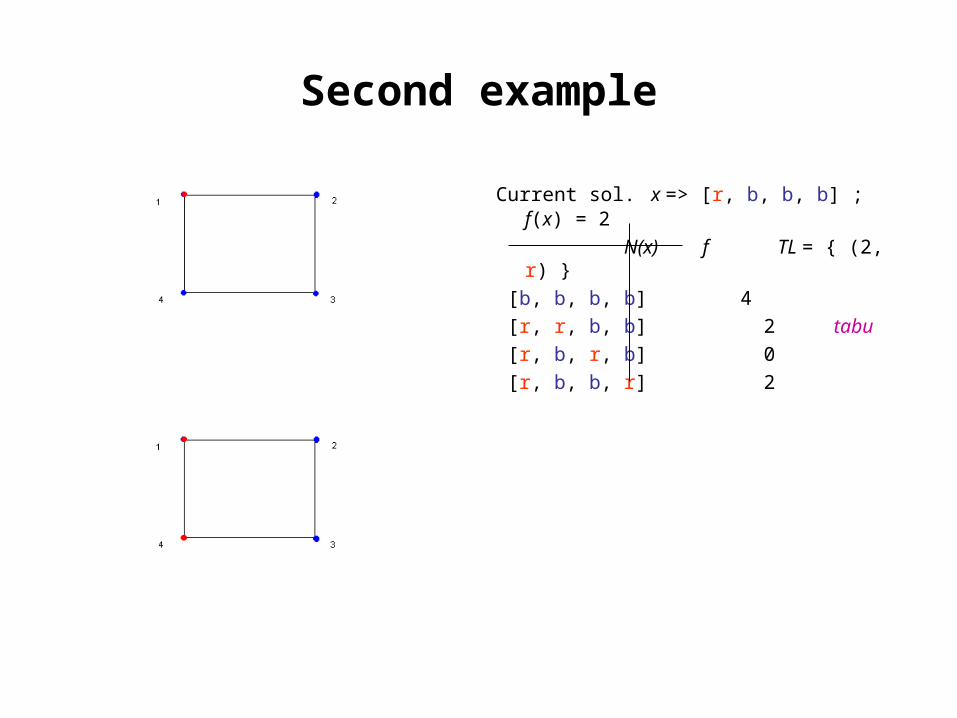
Second example
Current sol. x => [r, b, b, b] ; f(x) = 2
N(x) f TL = { (2, r) }
[b, b, b, b] 4
[r, r, b, b] 2 tabu
[r, b, r, b] 0
[r, b, b, r] 2
• x' => [r, b, r, b] ; f(x') = 0
• Since f(x') = 0 then
the procedure stops with
x* = x' => [r, b, r, b]
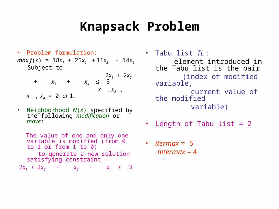
Knapsack Problem
• Problem formulation:max f(x) = 18x1 + 25x2 + 11x3 + 14x4
Subject to 2x1 + 2x2 + x3 + x4 ≤ 3 x1 , x2 , x3 , x4 = 0 or 1.
• Neighborhood N(x) specified by the following modification or move:
The value of one and only one variable is modified (from 0 to 1 or from 1 to 0)
to generate a new solution satisfying constraint
2x1 + 2x2 + x3 + x4 ≤ 3
• Tabu list TL : element introduced in the Tabu list is
the pair (index of modified variable, current value of the modified variable)
• Length of Tabu list = 2
• itermax = 5 nitermax = 4
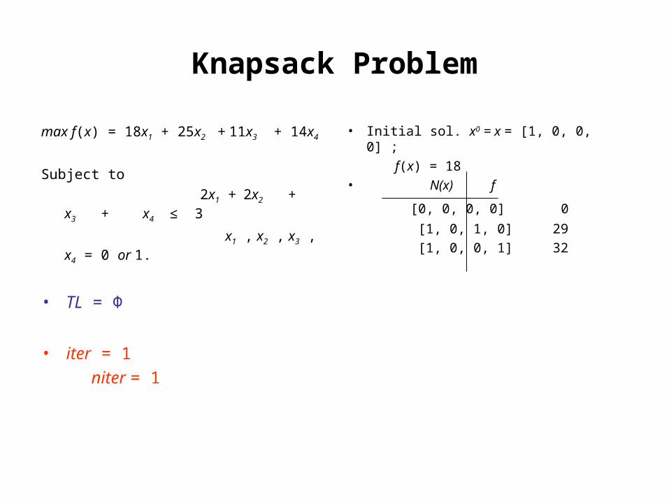
Knapsack Problem
max f(x) = 18x1 + 25x2 + 11x3 + 14x4
Subject to
2x1 + 2x2 + x3 + x4 ≤ 3
x1 , x2 , x3 , x4 = 0 or 1.
• TL = Φ
• iter = 1
niter = 1
• Initial sol. x0 = x = [1, 0, 0, 0] ;
f(x) = 18• N(x) f
[0, 0, 0, 0] 0
[1, 0, 1, 0] 29
[1, 0, 0, 1] 32
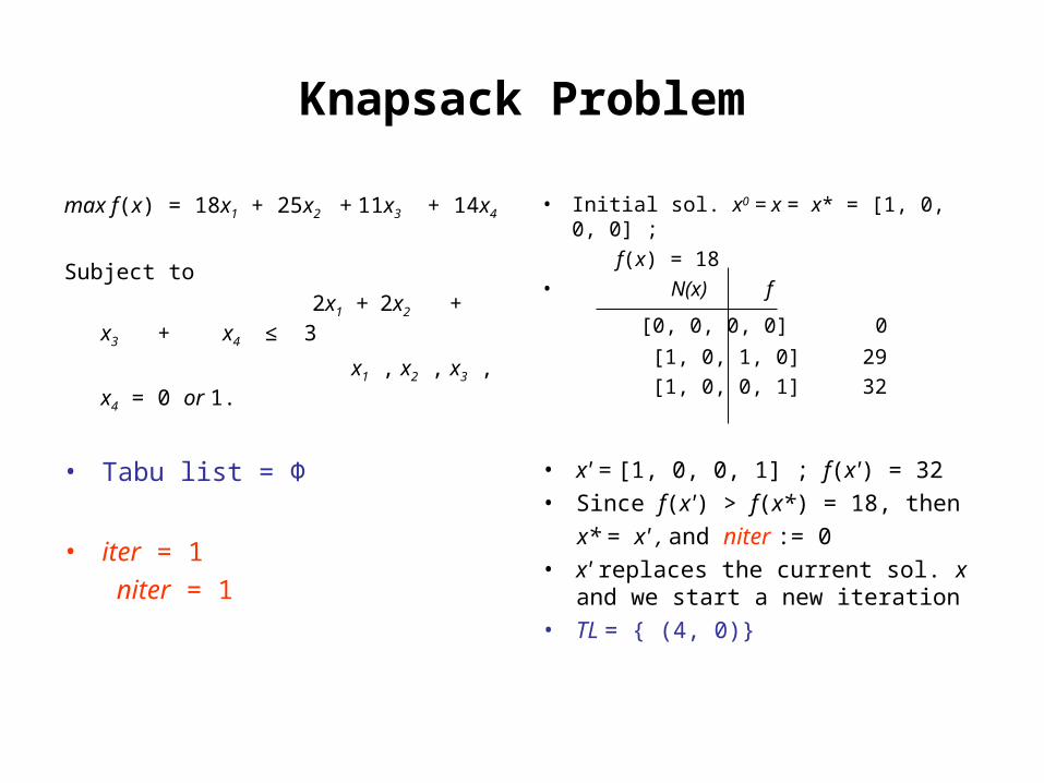
Knapsack Problem
max f(x) = 18x1 + 25x2 + 11x3 + 14x4
Subject to
2x1 + 2x2 + x3 + x4 ≤ 3
x1 , x2 , x3 , x4 = 0 or 1.
• Initial sol. x0 = x = x* = [1, 0, 0, 0] ;
f(x) = 18• N(x) f
[0, 0, 0, 0] 0
[1, 0, 1, 0] 29
[1, 0, 0, 1] 32
• x' = [1, 0, 0, 1] ; f(x') = 32
• Since f(x') > f(x*) = 18, then
x* = x' , and niter := 0
• x' replaces the current sol. x and we start a new iteration
• TL = { (4, 0)}
• Tabu list = Φ
• iter = 1
niter = 1
Knapsack Problem
max f(x) = 18x1 + 25x2 + 11x3 + 14x4
Subject to
2x1 + 2x2 + x3 + x4 ≤ 3
x1 , x2 , x3 , x4 = 0 or 1.
• Current sol. x = [1, 0, 0, 1] ;
f(x) = 32
• N(x) f
[0, 0, 0, 1] 14
[1, 0, 0, 0] 18 <= tabu
• TL = { (4, 0)}
• iter = 2
niter = 1
Knapsack Problem
max f(x) = 18x1 + 25x2 + 11x3 + 14x4
Subject to
2x1 + 2x2 + x3 + x4 ≤ 3
x1 , x2 , x3 , x4 = 0 or 1.
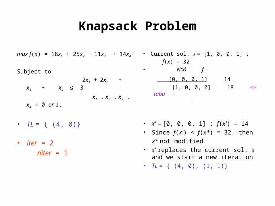
• Current sol. x = [1, 0, 0, 1] ;
f(x) = 32• N(x) f
[0, 0, 0, 1] 14
[1, 0, 0, 0] 18 <= tabu
• x' = [0, 0, 0, 1] ; f(x') = 14
• Since f(x') < f(x*) = 32, then
x* not modified
• x' replaces the current sol. x and we start a new iteration
• TL = { (4, 0), (1, 1)}
• TL = { (4, 0)}
• iter = 2
niter = 1
Knapsack Problem
max f(x) = 18x1 + 25x2 + 11x3 + 14x4
Subject to
2x1 + 2x2 + x3 + x4 ≤ 3
x1 , x2 , x3 , x4 = 0 or 1.
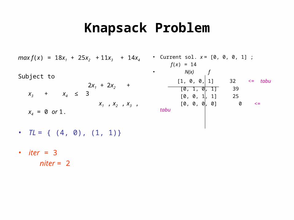
• Current sol. x = [0, 0, 0, 1] ;
f(x) = 14• N(x) f
[1, 0, 0, 1] 32 <= tabu
[0, 1, 0, 1] 39
[0, 0, 1, 1] 25
[0, 0, 0, 0] 0 <= tabu
• TL = { (4, 0), (1, 1)}
• iter = 3
niter = 2
Knapsack Problem
max f(x) = 18x1 + 25x2 + 11x3 + 14x4
Subject to
2x1 + 2x2 + x3 + x4 ≤ 3
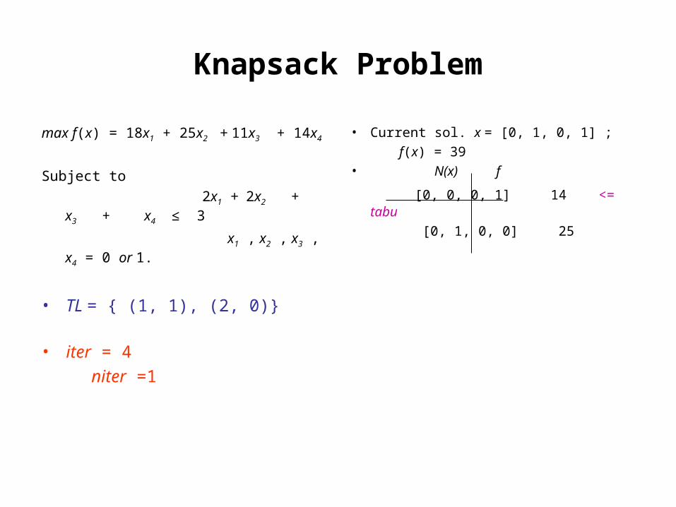
x1 , x2 , x3 , x4 = 0 or 1.
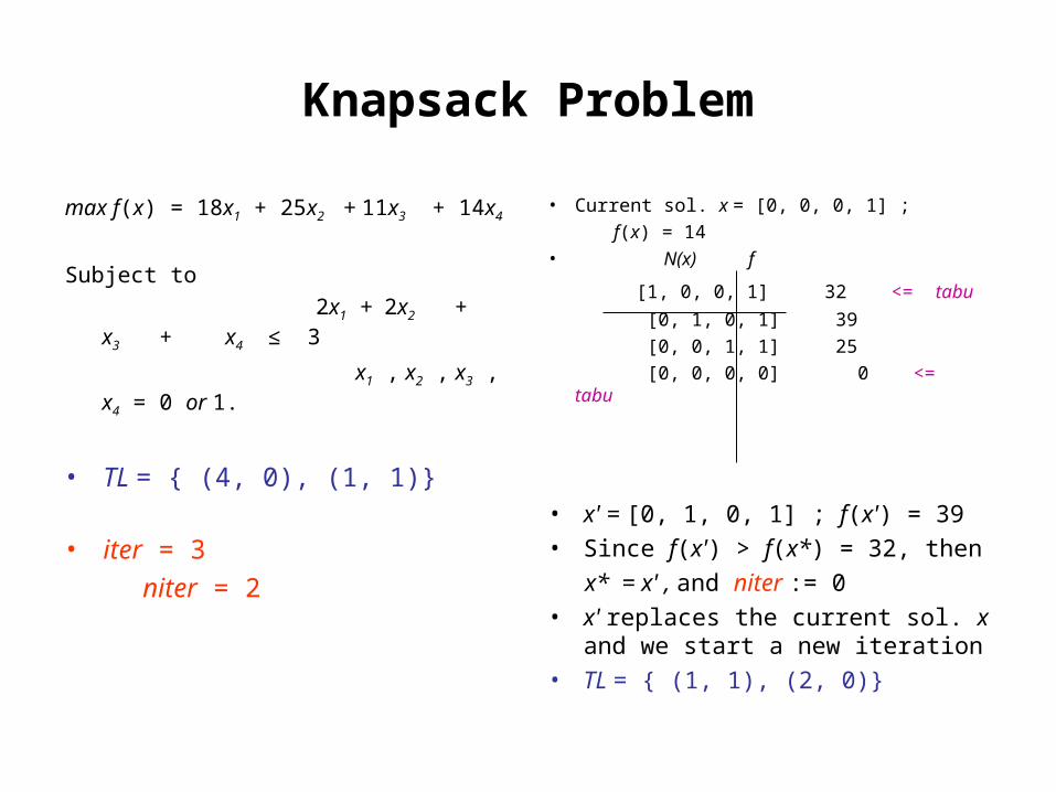
• Current sol. x = [0, 0, 0, 1] ;
f(x) = 14• N(x) f
[1, 0, 0, 1] 32 <= tabu
[0, 1, 0, 1] 39
[0, 0, 1, 1] 25
[0, 0, 0, 0] 0 <= tabu
• x' = [0, 1, 0, 1] ; f(x') = 39
• Since f(x') > f(x*) = 32, then
x* = x' , and niter := 0
• x' replaces the current sol. x and we start a new iteration
• TL = { (1, 1), (2, 0)}
• TL = { (4, 0), (1, 1)}
• iter = 3
niter = 2
Knapsack Problem
max f(x) = 18x1 + 25x2 + 11x3 + 14x4
Subject to
2x1 + 2x2 + x3 + x4 ≤ 3
x1 , x2 , x3 , x4 = 0 or 1.
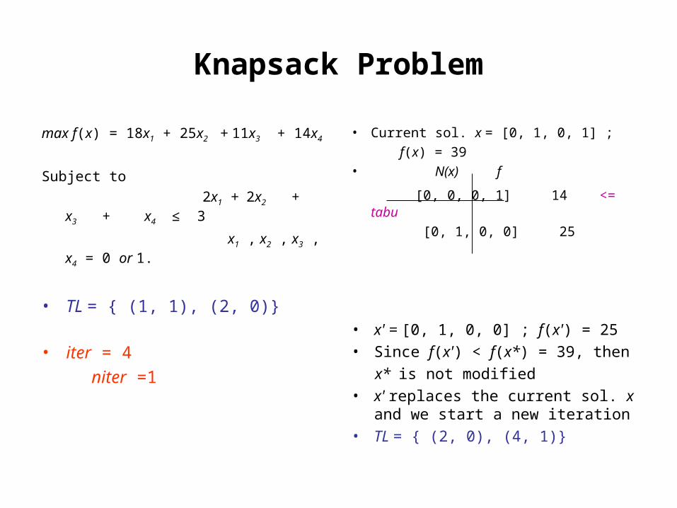
• Current sol. x = [0, 1, 0, 1] ;
f(x) = 39• N(x) f
[0, 0, 0, 1] 14 <= tabu
[0, 1, 0, 0] 25
• TL = { (1, 1), (2, 0)}
• iter = 4
niter =1
Knapsack Problem
max f(x) = 18x1 + 25x2 + 11x3 + 14x4
Subject to
2x1 + 2x2 + x3 + x4 ≤ 3
x1 , x2 , x3 , x4 = 0 or 1.
• Current sol. x = [0, 1, 0, 1] ;
f(x) = 39• N(x) f
[0, 0, 0, 1] 14 <= tabu
[0, 1, 0, 0] 25
• x' = [0, 1, 0, 0] ; f(x') = 25
• Since f(x') < f(x*) = 39, then
x* is not modified
• x' replaces the current sol. x and we start a new iteration
• TL = { (2, 0), (4, 1)}
• TL = { (1, 1), (2, 0)}
• iter = 4
niter =1
Knapsack Problem
max f(x) = 18x1 + 25x2 + 11x3 + 14x4
Subject to
2x1 + 2x2 + x3 + x4 ≤ 3
x1 , x2 , x3 , x4 = 0 or 1.
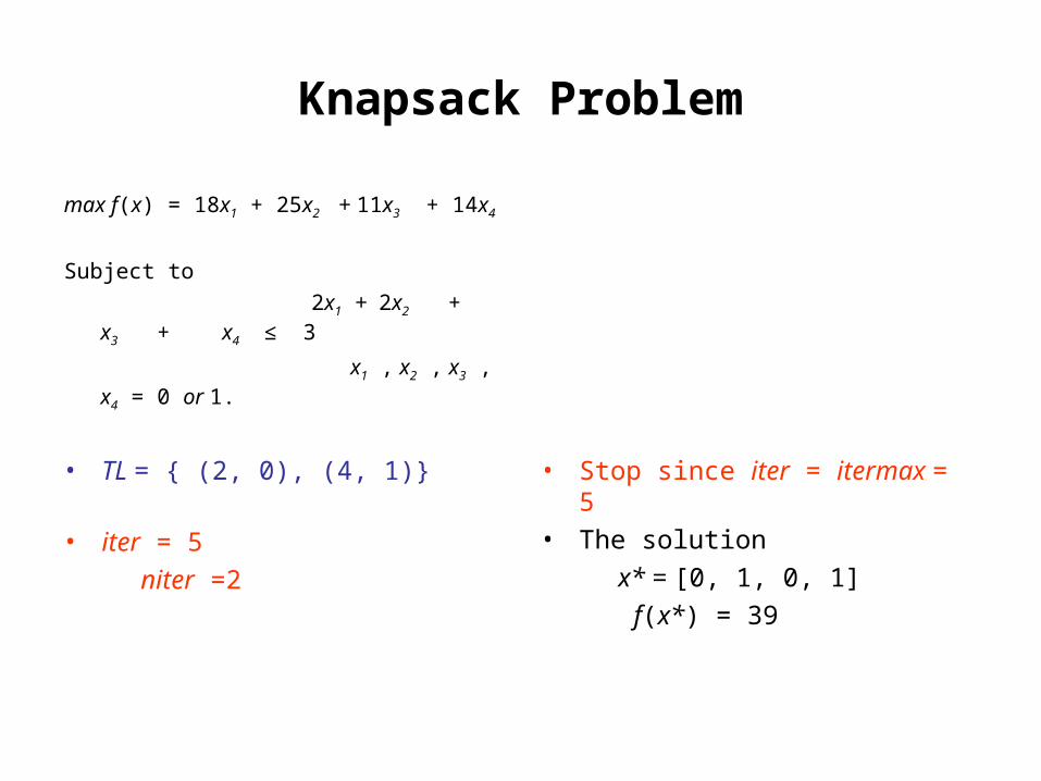
• TL = { (2, 0), (4, 1)}
• iter = 5
niter =2
• Stop since iter = itermax = 5
• The solution
x* = [0, 1, 0, 1]
f(x*) = 39
Simulated Annealing
• Probabilistic technique allowing to move out of local minima
• At each iteration, a solution x' is selected randomly in a subset of the neighborhood N(x)
• This approach was already used to simulate the evolution of an unstable physical system toward a thermodynamic stable equilibrium point at a fixed temperature
Simulated Annealing
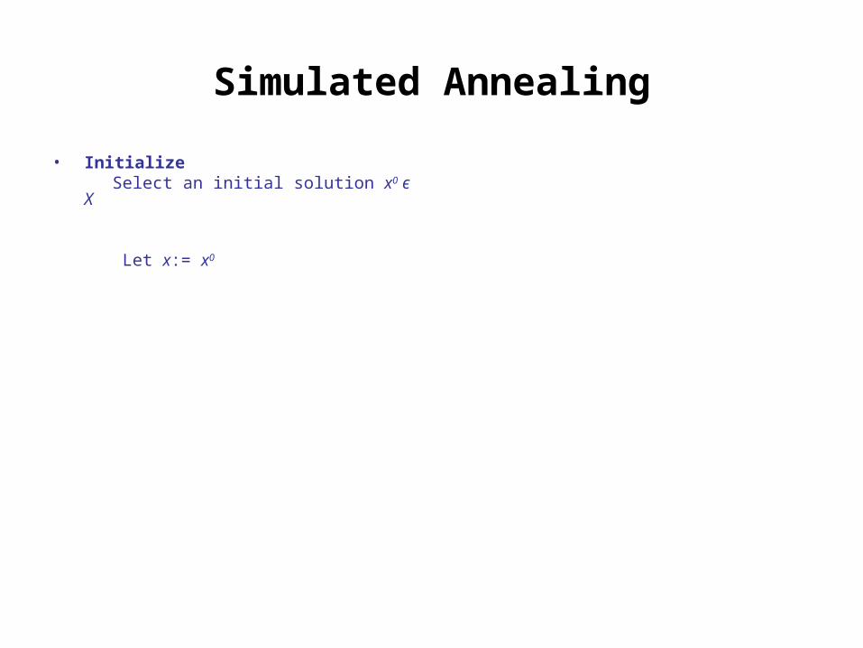
• Initialize Select an initial solution x0 є X
Let x:= x0
Simulated Annealing
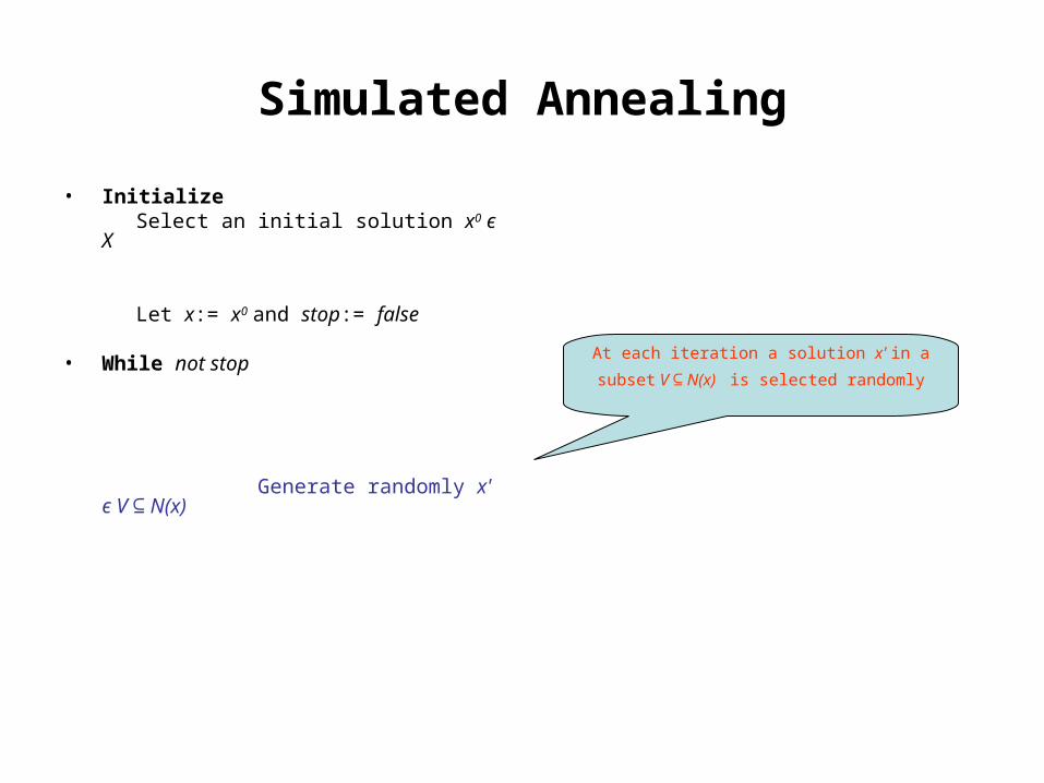
• Initialize Select an initial solution x0 є X
Let x:= x0 and stop:= false
• While not stop
Generate randomly x' є V N(x)⊆
At each iteration a solution x' in a subset
V N(x)⊆ is selected randomly
Simulated Annealing
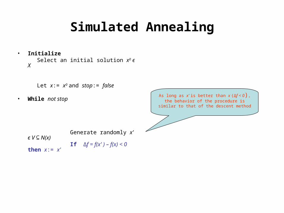
• Initialize Select an initial solution x0 є X
Let x:= x0 and stop:= false
• While not stop
Generate randomly x' є V N(x)⊆ If ∆f = f(x' ) – f(x) < 0 then x:= x'
As long as x' is better than x (∆f < 0), the behavior of the procedure is similar to
that of the descent method
Simulated Annealing
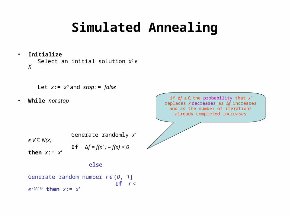
• Initialize Select an initial solution x0 є X
Let x:= x0 and stop:= false
• While not stop
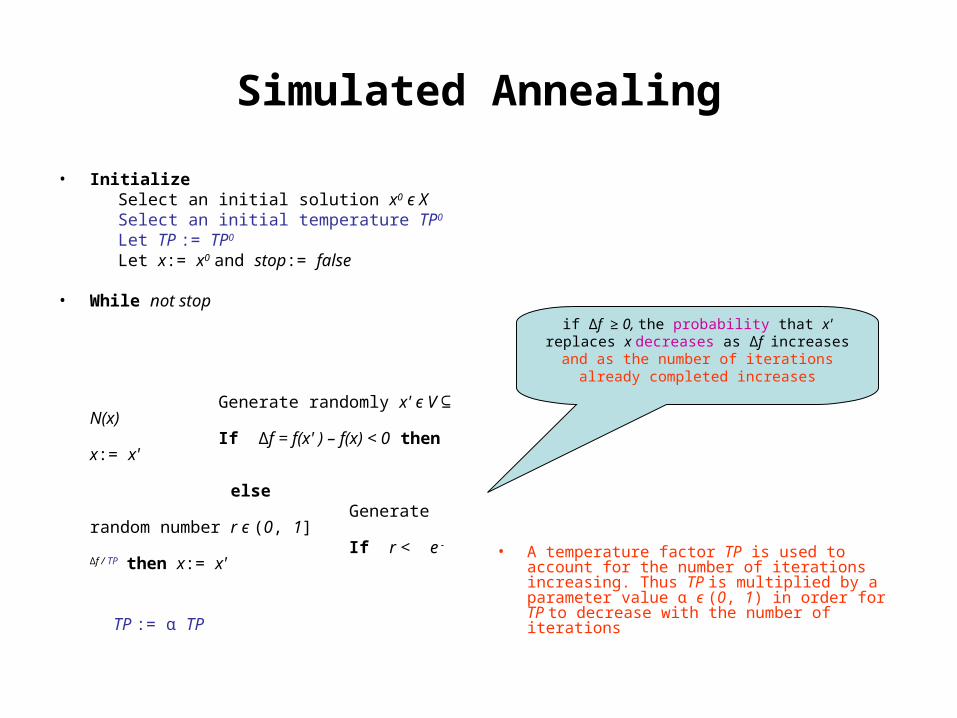
Generate randomly x' є V N(x)⊆ If ∆f = f(x' ) – f(x) < 0 then x:= x' else Generate random number r є (0, 1] If r < e - ∆f / TP then x:= x'
if ∆f ≥ 0, the probability that x' replaces x decreases as ∆f increases and as the number
of iterations already completed increases
Simulated Annealing
• Initialize Select an initial solution x0 є X Select an initial temperature TP0
Let TP := TP0
Let x:= x0 and stop:= false
• While not stop
Generate randomly x' є V N(x)⊆ If ∆f = f(x' ) – f(x) < 0 then x:= x' else Generate random number r є (0, 1] If r < e - ∆f / TP then x:= x'
TP := α TP
• A temperature factor TP is used to account for the number of iterations increasing. Thus TP is multiplied by a parameter value α є (0, 1) in order for TP to decrease with the number of iterations
if ∆f ≥ 0, the probability that x' replaces x decreases as ∆f increases and as the number
of iterations already completed increases
Simulated Annealing
• Initialize Select an initial solution x0 є X Select an initial temperature TP0
Let TP := TP0
Let x:= x0 and stop:= false
• While not stop
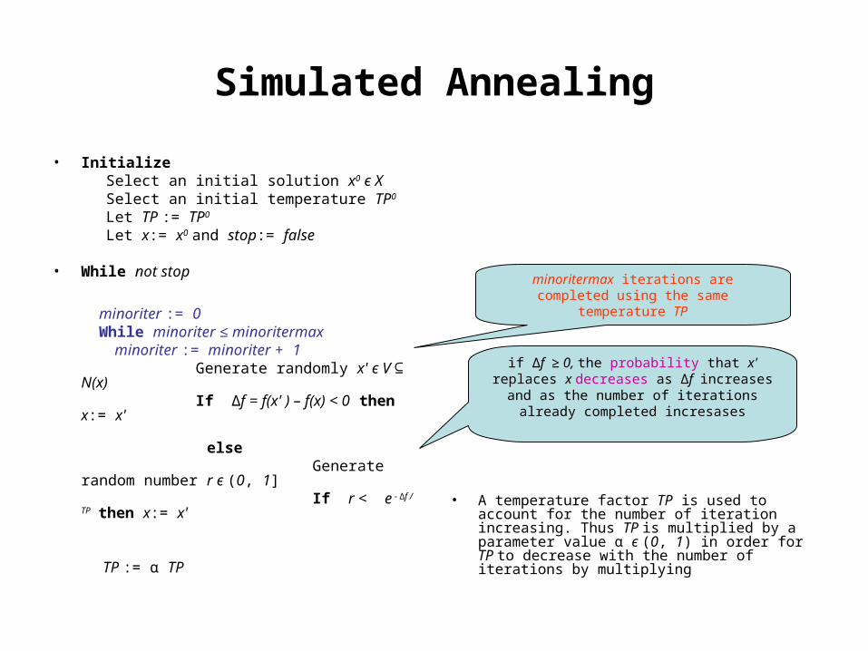
minoriter := 0 While minoriter ≤ minoritermax minoriter := minoriter + 1 Generate randomly x' є V N(x)⊆ If ∆f = f(x' ) – f(x) < 0 then x:= x' else Generate random number r є (0, 1] If r < e - ∆f / TP then x:= x'
TP := α TP
• A temperature factor TP is used to account for the number of iteration increasing. Thus TP is multiplied by a parameter value α є (0, 1) in order for TP to decrease with the number of iterations by multiplying
if ∆f ≥ 0, the probability that x' replaces x decreases as ∆f increases and as the
number of iterations already completed incresases
minoritermax iterations are completed using the same temperature TP
Simulated Annealing
• Initialize Select an initial solution x0 є X Select an initial temperature TP0
Let TP := TP0
Let x* := x:= x0 and stop:= false
• While not stop
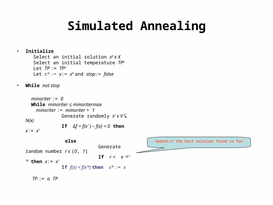
minoriter := 0 While minoriter ≤ minoritermax minoriter := minoriter + 1 Generate randomly x' є V N(x)⊆ If ∆f = f(x' ) – f(x) < 0 then x:= x' else Generate random number r є (0, 1] If r < e - ∆f / TP then x:= x' If f(x) < f(x*) then x* := x
TP := α TP
Update x* the best solution found so far
Simulated Annealing
• Initialize Select an initial solution x0 є X Select an initial temperature TP0
Let TP := TP0
Let x* := x:= x0 and stop:= false
• While not stop
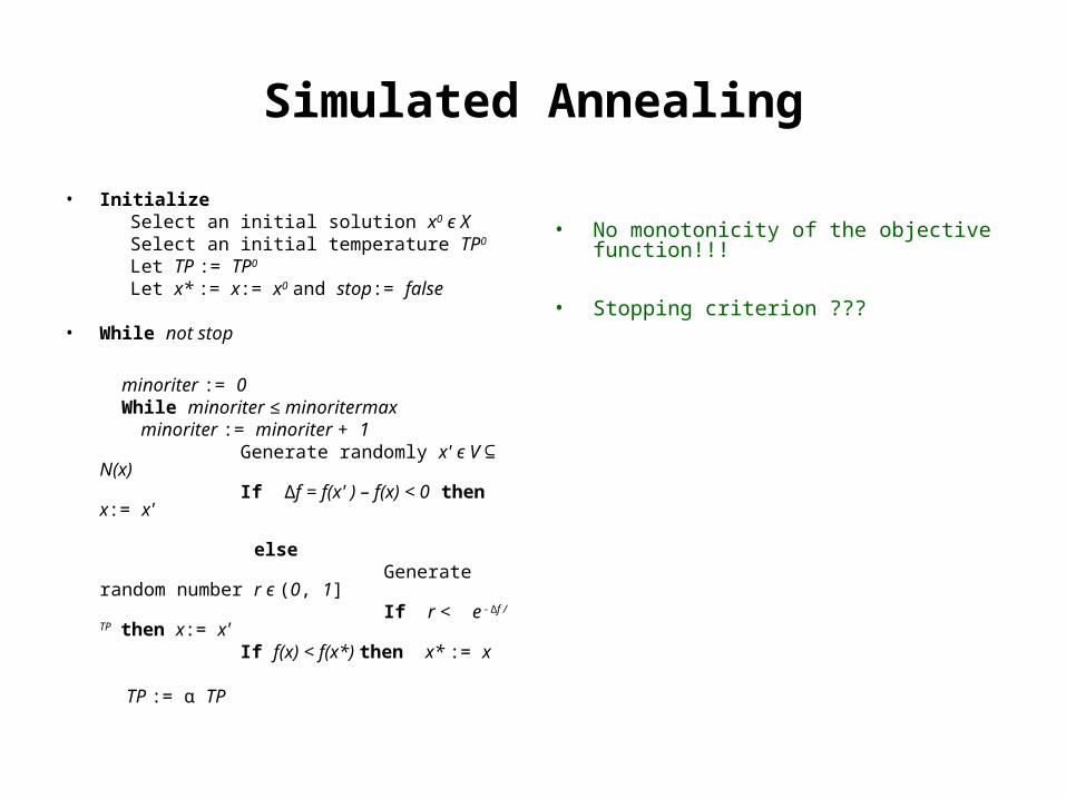
minoriter := 0 While minoriter ≤ minoritermax minoriter := minoriter + 1 Generate randomly x' є V N(x)⊆ If ∆f = f(x' ) – f(x) < 0 then x:= x' else Generate random number r є (0, 1] If r < e - ∆f / TP then x:= x' If f(x) < f(x*) then x* := x
TP := α TP
• No monotonicity of the objective function!!!
• Stopping criterion ???
Simulated Annealing
• Initialize Select an initial solution x0 є X Select an initial temperature TP0
Let iter := niter := 0 and TP := TP0
Let x* := x:= x0 and stop:= false
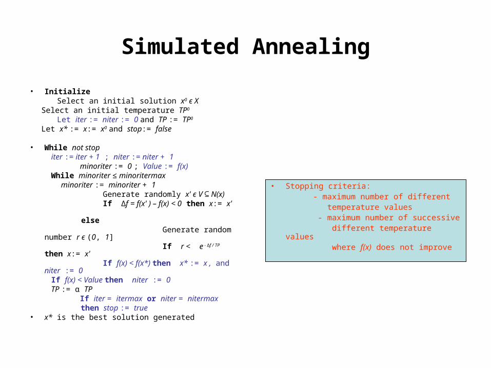
• While not stop iter := iter + 1 ; niter := niter + 1 minoriter := 0 ; Value := f(x) While minoriter ≤ minoritermax minoriter := minoriter + 1 Generate randomly x' є V N(x)⊆ If ∆f = f(x' ) – f(x) < 0 then x:= x' else Generate random number r є (0, 1] If r < e - ∆f / TP then x:= x' If f(x) < f(x*) then x* := x , and niter := 0 If f(x) < Value then niter := 0 TP := α TP If iter = itermax or niter = nitermax then stop := true• x* is the best solution generated
• Stopping criteria: - maximum number of different temperature values - maximum number of successive different temperature values where f(x) does not improve
Knapsack Problem
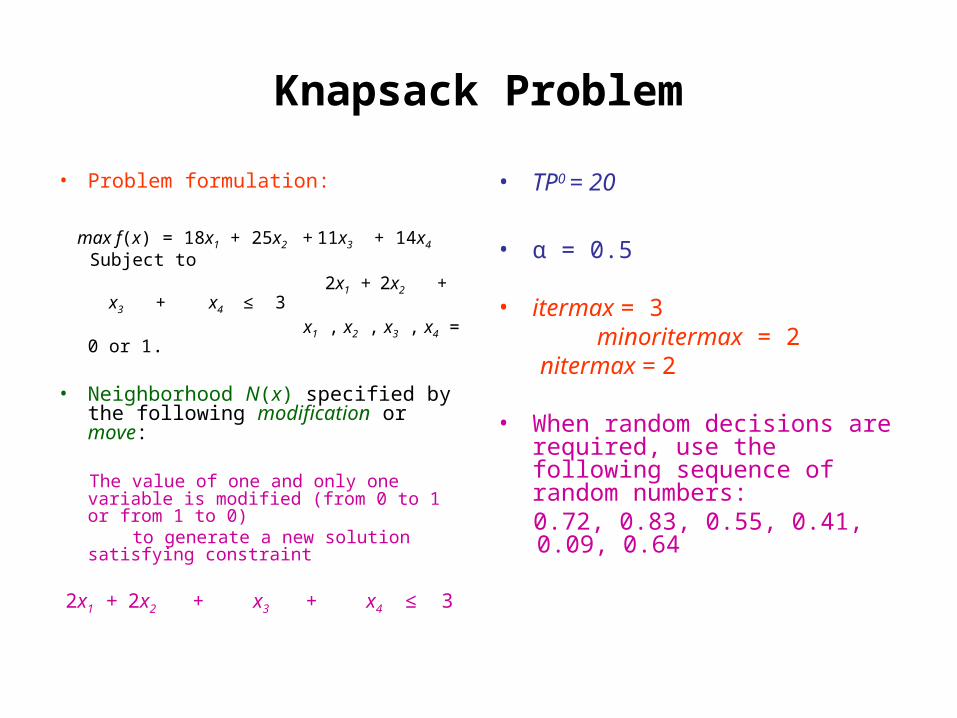
• Problem formulation:
max f(x) = 18x1 + 25x2 + 11x3 + 14x4 Subject to 2x1 + 2x2 + x3 + x4 ≤ 3
x1 , x2 , x3 , x4 = 0 or 1.
• Neighborhood N(x) specified by the following modification or move:
The value of one and only one variable is modified (from 0 to 1 or from 1 to 0)
to generate a new solution satisfying constraint
2x1 + 2x2 + x3 + x4 ≤ 3
• TP0 = 20
• α = 0.5
• itermax = 3 minoritermax = 2 nitermax = 2
• When random decisions are required, use the following sequence of random numbers:
0.72, 0.83, 0.55, 0.41, 0.09, 0.64
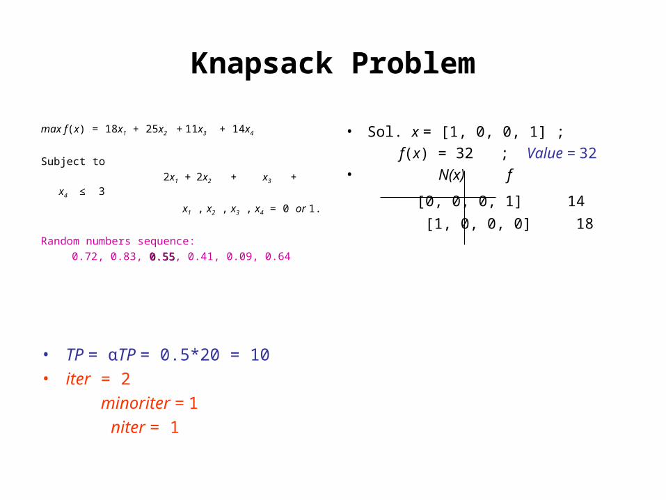
Knapsack Problem
max f(x) = 18x1 + 25x2 + 11x3 + 14x4
Subject to
2x1 + 2x2 + x3 + x4 ≤ 3
x1 , x2 , x3 , x4 = 0 or 1.
Random numbers sequence:
0.72, 0.83, 0.550.55, 0.41, 0.09, 0.64
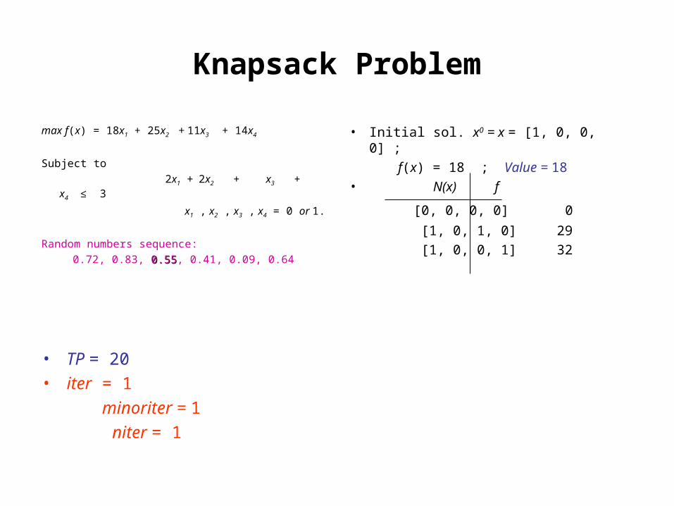
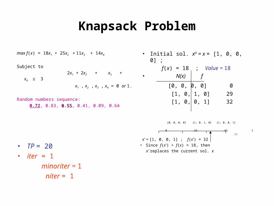
• Initial sol. x0 = x = [1, 0, 0, 0] ;
f(x) = 18 ; Value = 18• N(x) f
[0, 0, 0, 0] 0
[1, 0, 1, 0] 29
[1, 0, 0, 1] 32
• TP = 20
• iter = 1
minoriter = 1
niter = 1
Knapsack Problem
max f(x) = 18x1 + 25x2 + 11x3 + 14x4
Subject to
2x1 + 2x2 + x3 + x4 ≤ 3
x1 , x2 , x3 , x4 = 0 or 1.
Random numbers sequence:
0.72, 0.83, 0.550.55, 0.41, 0.09, 0.64
• TP = 20
• iter = 1
minoriter = 1
niter = 1
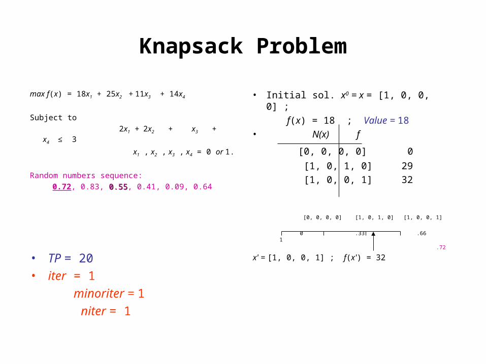
• Initial sol. x0 = x = [1, 0, 0, 0] ;
f(x) = 18 ; Value = 18• N(x) f
[0, 0, 0, 0] 0
[1, 0, 1, 0] 29
[1, 0, 0, 1] 32
[0, 0, 0, 0] [1, 0, 1, 0] [1, 0, 0, 1]
0 .33 .66 1
.72
x' = [1, 0, 0, 1] ; f(x') = 32
Knapsack Problem
max f(x) = 18x1 + 25x2 + 11x3 + 14x4
Subject to
2x1 + 2x2 + x3 + x4 ≤ 3
x1 , x2 , x3 , x4 = 0 or 1.
Random numbers sequence:
0.72, 0.83, 0.550.55, 0.41, 0.09, 0.64
• TP = 20
• iter = 1
minoriter = 1
niter = 1
• Initial sol. x0 = x = [1, 0, 0, 0] ;
f(x) = 18 ; Value = 18• N(x) f
[0, 0, 0, 0] 0
[1, 0, 1, 0] 29
[1, 0, 0, 1] 32
[0, 0, 0, 0] [1, 0, 1, 0] [1, 0, 0, 1]
0 .33 .66 1
.72
x' = [1, 0, 0, 1] ; f(x') = 32• Since f(x') > f(x) = 18, then
x' replaces the current sol. x
Knapsack Problem
max f(x) = 18x1 + 25x2 + 11x3 + 14x4
Subject to
2x1 + 2x2 + x3 + x4 ≤ 3
x1 , x2 , x3 , x4 = 0 or 1.
Random numbers sequence:
0.72, 0.83, 0.550.55, 0.41, 0.09, 0.64
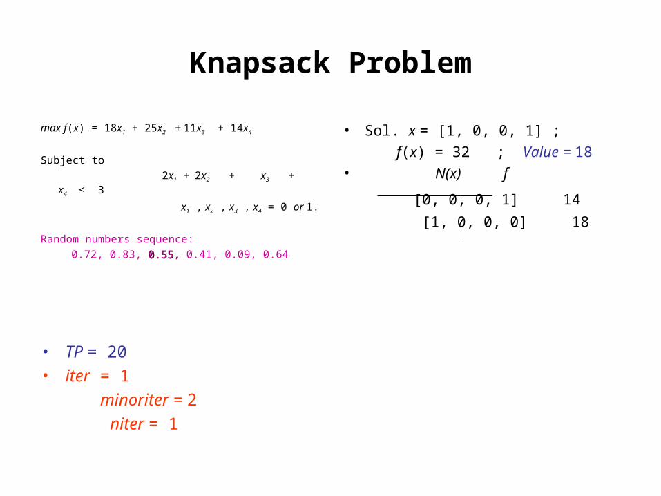
• Sol. x = [1, 0, 0, 1] ;
f(x) = 32 ; Value = 18• N(x) f
[0, 0, 0, 1] 14
[1, 0, 0, 0] 18
• TP = 20
• iter = 1
minoriter = 2
niter = 1
Knapsack Problem
max f(x) = 18x1 + 25x2 + 11x3 + 14x4
Subject to
2x1 + 2x2 + x3 + x4 ≤ 3
x1 , x2 , x3 , x4 = 0 or 1.
Random numbers sequence:
0.72, 0.83, 0.550.55, 0.41, 0.09, 0.64
• TP = 20
• iter = 1
minoriter = 2
niter = 1
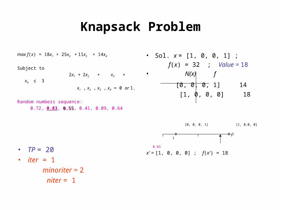
• Sol. x = [1, 0, 0, 1] ;
f(x) = 32 ; Value = 18• N(x) f
[0, 0, 0, 1] 14
[1, 0, 0, 0] 18
[0, 0, 0, 1] [1, 0,0, 0]
0 0.5 1
0.83
x' = [1, 0, 0, 0] ; f(x') = 18
Knapsack Problem
max f(x) = 18x1 + 25x2 + 11x3 + 14x4
Subject to
2x1 + 2x2 + x3 + x4 ≤ 3
x1 , x2 , x3 , x4 = 0 or 1.
Random numbers sequence:
0.72, 0.83, 0.55, 0.41, 0.09, 0.64
• TP = 20
• iter = 1
minoriter = 2
niter = 1
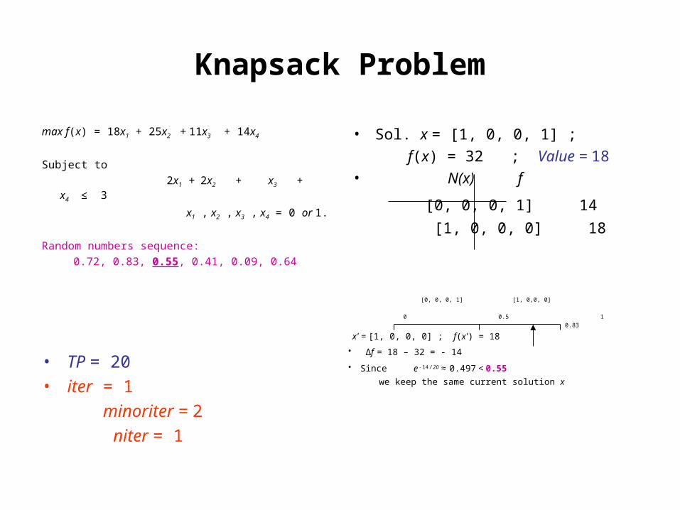
• Sol. x = [1, 0, 0, 1] ;
f(x) = 32 ; Value = 18• N(x) f
[0, 0, 0, 1] 14
[1, 0, 0, 0] 18
[0, 0, 0, 1] [1, 0,0, 0]
0 0.5 1
0.83
x' = [1, 0, 0, 0] ; f(x') = 18
• ∆f = 18 – 32 = - 14
• Since e - 14 / 20 ≈ 0.497 < 0.55
we keep the same current solution x
Knapsack Problem
max f(x) = 18x1 + 25x2 + 11x3 + 14x4
Subject to
2x1 + 2x2 + x3 + x4 ≤ 3
x1 , x2 , x3 , x4 = 0 or 1.
Random numbers sequence:
0.72, 0.83, 0.550.55, 0.41, 0.09, 0.64
• Sol. x = [1, 0, 0, 1] ;
f(x) = 32 ; Value = 32• N(x) f
[0, 0, 0, 1] 14
[1, 0, 0, 0] 18
• TP = αTP = 0.5*20 = 10
• iter = 2
minoriter = 1
niter = 1
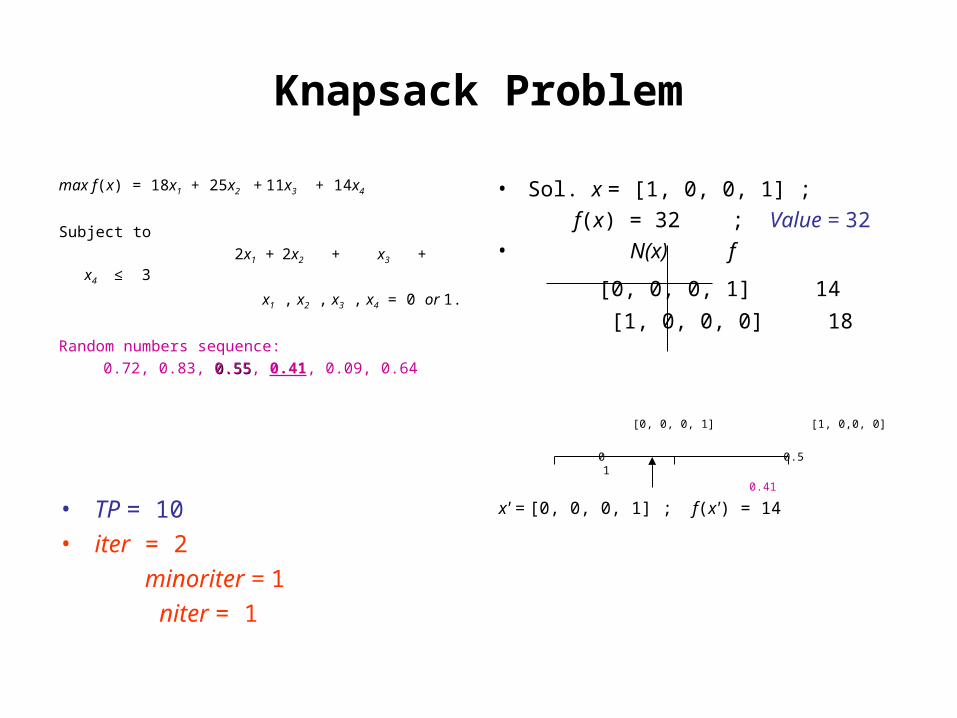
Knapsack Problem
max f(x) = 18x1 + 25x2 + 11x3 + 14x4
Subject to
2x1 + 2x2 + x3 + x4 ≤ 3
x1 , x2 , x3 , x4 = 0 or 1.
Random numbers sequence:
0.72, 0.83, 0.550.55, 0.41, 0.09, 0.64
• TP = 10
• iter = 2
minoriter = 1
niter = 1
• Sol. x = [1, 0, 0, 1] ;
f(x) = 32 ; Value = 32• N(x) f
[0, 0, 0, 1] 14
[1, 0, 0, 0] 18
[0, 0, 0, 1] [1, 0,0, 0]
0 0.5 1
0.41
x' = [0, 0, 0, 1] ; f(x') = 14
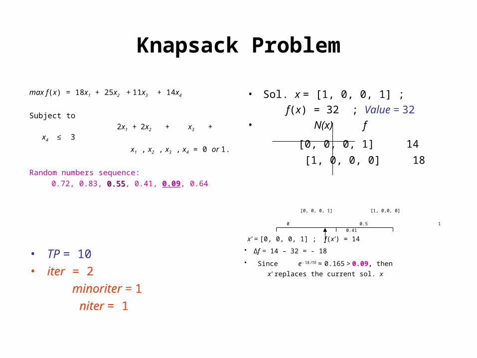
• ∆f = 14 – 32 = - 18
• Since e - 18 /10 ≈ 0.165 > 0.09, then
x' replaces the current sol. x
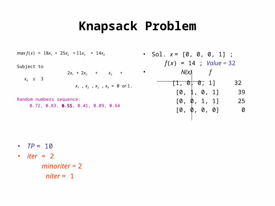
Knapsack Problem
max f(x) = 18x1 + 25x2 + 11x3 + 14x4
Subject to
2x1 + 2x2 + x3 + x4 ≤ 3
x1 , x2 , x3 , x4 = 0 or 1.
Random numbers sequence:
0.72, 0.83, 0.550.55, 0.41, 0.09, 0.64
• Sol. x = [0, 0, 0, 1] ;
f(x) = 14 ; Value = 32• N(x) f
[1, 0, 0, 1] 32
[0, 1, 0, 1] 39
[0, 0, 1, 1] 25
[0, 0, 0, 0] 0
• TP = 10
• iter = 2
minoriter = 2
niter = 1
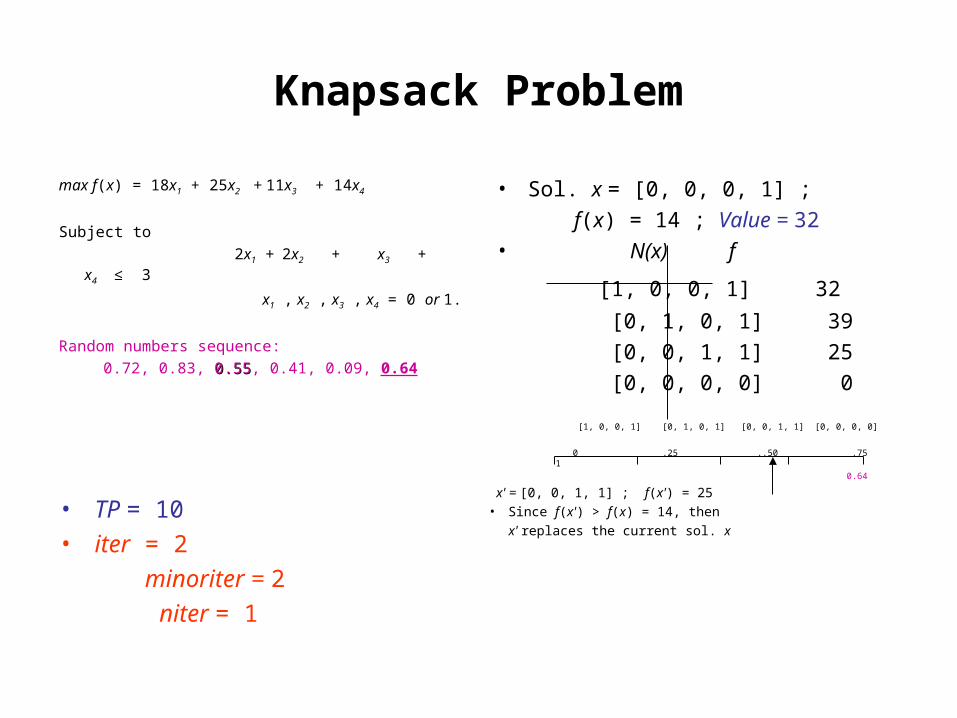
Knapsack Problem
max f(x) = 18x1 + 25x2 + 11x3 + 14x4
Subject to
2x1 + 2x2 + x3 + x4 ≤ 3
x1 , x2 , x3 , x4 = 0 or 1.
Random numbers sequence:
0.72, 0.83, 0.550.55, 0.41, 0.09, 0.64
• TP = 10
• iter = 2
minoriter = 2
niter = 1
• Sol. x = [0, 0, 0, 1] ;
f(x) = 14 ; Value = 32• N(x) f
[1, 0, 0, 1] 32
[0, 1, 0, 1] 39
[0, 0, 1, 1] 25
[0, 0, 0, 0] 0
[1, 0, 0, 1] [0, 1, 0, 1] [0, 0, 1, 1] [0, 0, 0, 0]
0 .25 ..50 .75 1
0.64
x' = [0, 0, 1, 1] ; f(x') = 25• Since f(x') > f(x) = 14, then
x' replaces the current sol. x
Knapsack Problem
max f(x) = 18x1 + 25x2 + 11x3 + 14x4
Subject to
2x1 + 2x2 + x3 + x4 ≤ 3
x1 , x2 , x3 , x4 = 0 or 1.
Random numbers sequence:
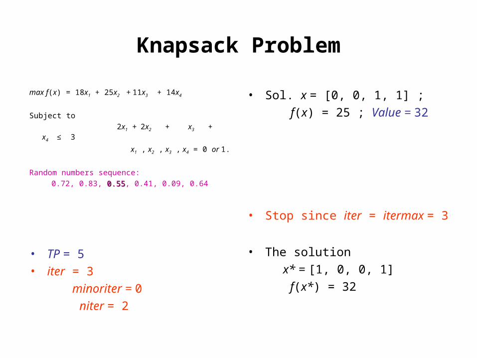
0.72, 0.83, 0.550.55, 0.41, 0.09, 0.64
• TP = 5
• iter = 3
minoriter = 0
niter = 2
• Sol. x = [0, 0, 1, 1] ;
f(x) = 25 ; Value = 32
• Stop since iter = itermax = 3
• The solution
x* = [1, 0, 0, 1]
f(x*) = 32
Threshold Accepting
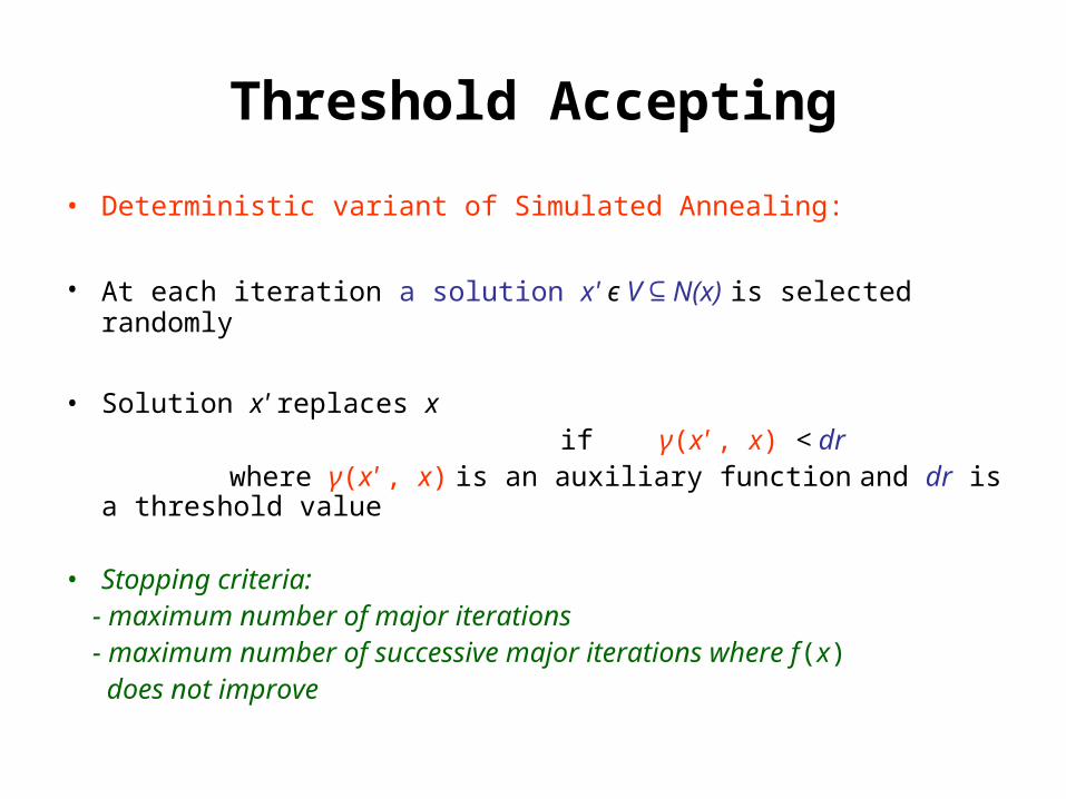
• Deterministic variant of Simulated Annealing:
• At each iteration a solution x' є V N(x)⊆ is selected randomly
• Solution x' replaces x if γ(x' , x) < dr where γ(x' , x) is an auxiliary function and dr is a threshold value
• Stopping criteria: - maximum number of major iterations - maximum number of successive major iterations where f(x) does not improve
Simulated Annealing vs Threshold Accepting
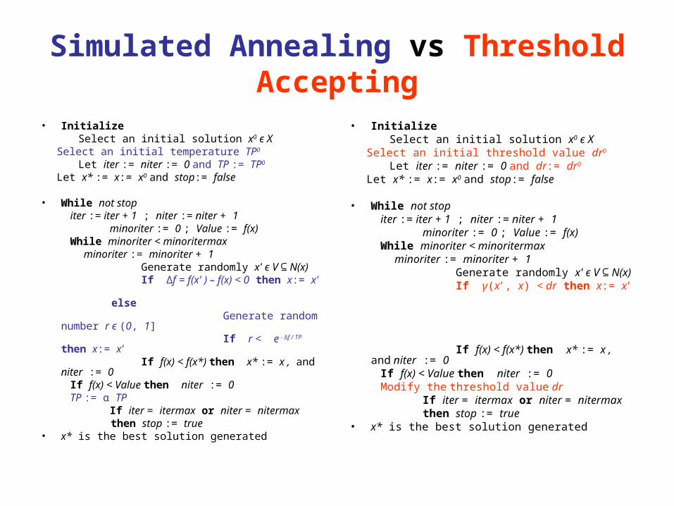
• Initialize Select an initial solution x0 є X Select an initial temperature TP0
Let iter := niter := 0 and TP := TP0
Let x* := x:= x0 and stop:= false
• While not stop iter := iter + 1 ; niter := niter + 1 minoriter := 0 ; Value := f(x) While minoriter < minoritermax minoriter := minoriter + 1 Generate randomly x' є V N(x)⊆ If ∆f = f(x' ) – f(x) < 0 then x:= x' else Generate random number r є (0, 1] If r < e - ∆f / TP then x:= x' If f(x) < f(x*) then x* := x , and niter := 0 If f(x) < Value then niter := 0 TP := α TP If iter = itermax or niter = nitermax then stop := true• x* is the best solution generated
• Initialize Select an initial solution x0 є X Select an initial threshold value dr0
Let iter := niter := 0 and dr:= dr0
Let x* := x:= x0 and stop:= false
• While not stop iter := iter + 1 ; niter := niter + 1 minoriter := 0 ; Value := f(x) While minoriter < minoritermax minoriter := minoriter + 1 Generate randomly x' є V N(x)⊆ If γ(x' , x) < dr then x:= x'
If f(x) < f(x*) then x* := x , and niter := 0 If f(x) < Value then niter := 0 Modify the threshold value dr If iter = itermax or niter = nitermax then stop := true• x* is the best solution generated
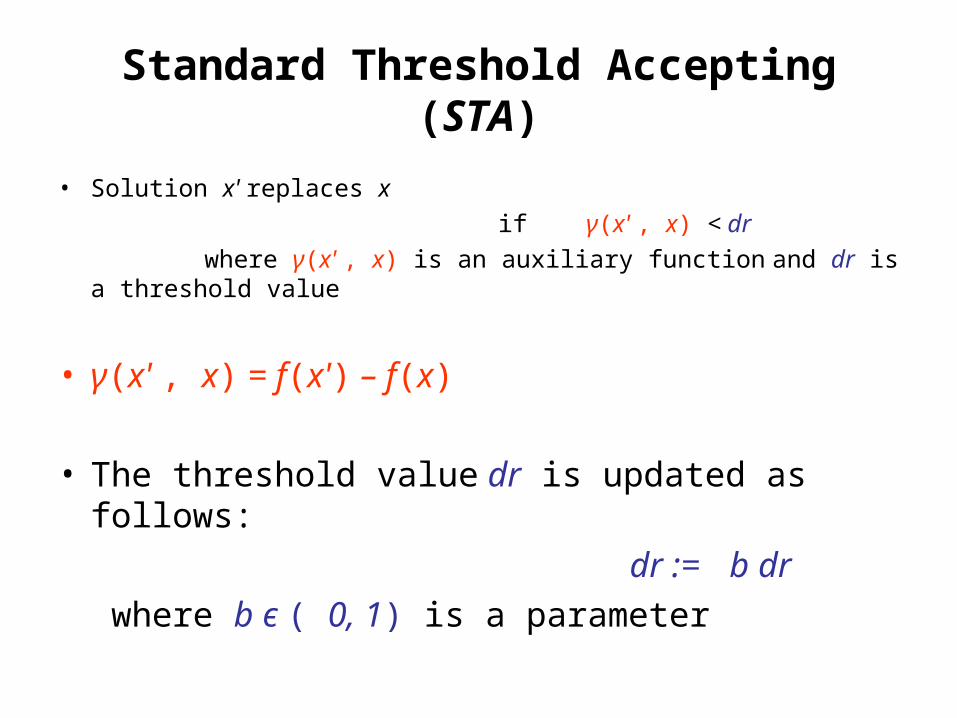
Standard Threshold Accepting (STA)
• Solution x' replaces x
if γ(x' , x) < dr
where γ(x' , x) is an auxiliary function and dr is a threshold value
• γ(x' , x) = f(x') – f(x)
• The threshold value dr is updated as follows:
dr := b dr
where b є ( 0, 1) is a parameter
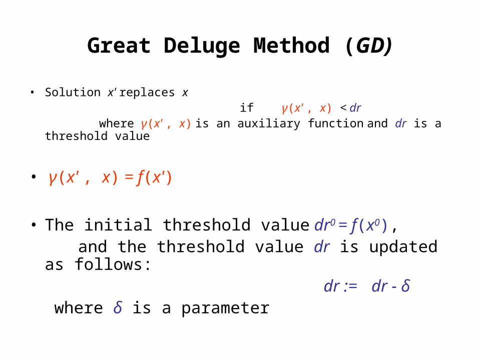
Great Deluge Method (GD)
• Solution x' replaces x if γ(x' , x) < dr where γ(x' , x) is an auxiliary function and dr is a threshold value
• γ(x' , x) = f(x')
• The initial threshold value dr0 = f(x0), and the threshold value dr is updated as follows: dr := dr - δ where δ is a parameter
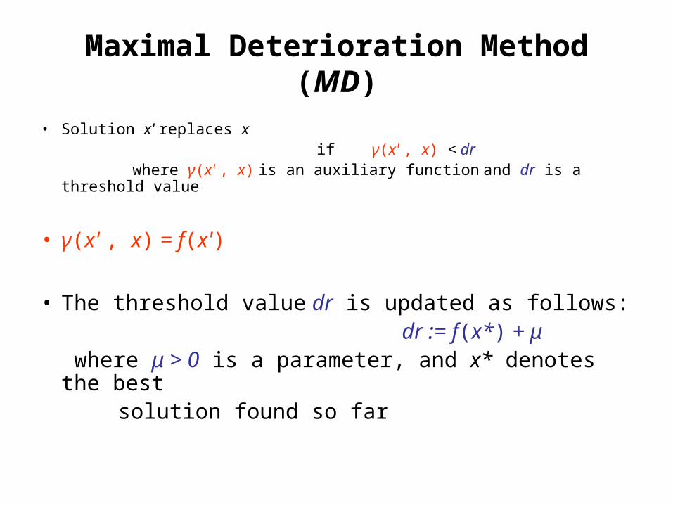
Maximal Deterioration Method (MD)
• Solution x' replaces x if γ(x' , x) < dr where γ(x' , x) is an auxiliary function and dr is a threshold value
• γ(x' , x) = f(x')
• The threshold value dr is updated as follows: dr := f(x*) + μ where μ > 0 is a parameter, and x* denotes the best solution found so far

Improving Strategies
• Intensification
• Multistart diversification strategies:
- Random Diversification (RD)
- First Order Diversification (FOD)
• Variable Neighborhood Search (VNS)
• Exchange Procedure
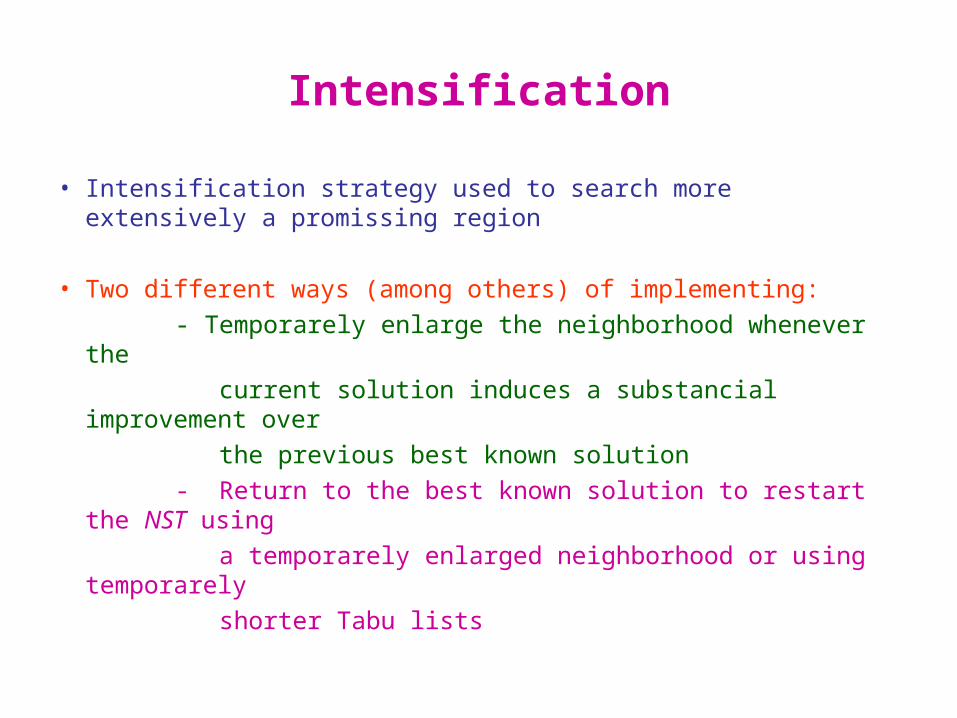
Intensification
• Intensification strategy used to search more extensively a promissing region
• Two different ways (among others) of implementing:
- Temporarely enlarge the neighborhood whenever the
current solution induces a substancial improvement over
the previous best known solution
- Return to the best known solution to restart the NST using
a temporarely enlarged neighborhood or using temporarely
shorter Tabu lists

Diversification
• The diversification principle is complementary to the intensification. Its objective is to search more extensively the feasible domain by leading the NST to unexplored regions of the feasible domain.
• Numerical experiences indicate that it seems better to apply a short NST (of shorter duration) several times using different initial solutions rather than a long NST (of longer duration).
Random Diversification (RD)
Multistart procedure using new initial solutions generated randomly (with GRASP for instance)

First Order Diversification (FOD)
• Multistart procedure using the current local minimum x* to generate a new initial solution
• Move away from x* by modifying the current resources of some activities in order to generate a new initial solution in such a way as to deteriorate the value of f as little as possible or even improve it, if possible
Variable Neighborhood Search (VNS)
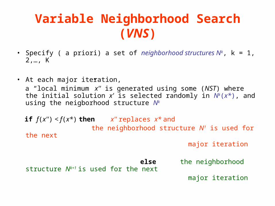
• Specify ( a priori) a set of neighborhood structures Nk, k = 1, 2,…, K
Variable Neighborhood Search (VNS)
• Specify ( a priori) a set of neighborhood structures Nk, k = 1, 2,…, K
• At each major iteration,
a “local minimum” x'' is generated using some (NST) where the initial solution x' is selected randomly in Nk(x*), and using the neigborhood structure Nk
Variable Neighborhood Search (VNS)
• Specify ( a priori) a set of neighborhood structures Nk, k = 1, 2,…, K
• At each major iteration, a “local minimum” x'' is generated using some (NST) where the initial
solution x' is selected randomly in Nk(x*), and using the neigborhood structure Nk
if f(x'') < f(x*) then x'' replaces x* and the neighborhood structure N1 is used for the next major iteration
Justification: we assume that it is easier to apply the NST with neighborhood structure N1
Variable Neighborhood Search (VNS)
• Specify ( a priori) a set of neighborhood structures Nk, k = 1, 2,…, K
• At each major iteration, a “local minimum” x'' is generated using some (NST) where the initial
solution x' is selected randomly in Nk(x*), and using the neigborhood structure Nk
if f(x'') < f(x*) then x'' replaces x* and the neighborhood structure N1 is used for the next major iteration
else the neighborhood structure Nk+1 is used for the next major iteration
Recall:Neighborhood for assignment type problem
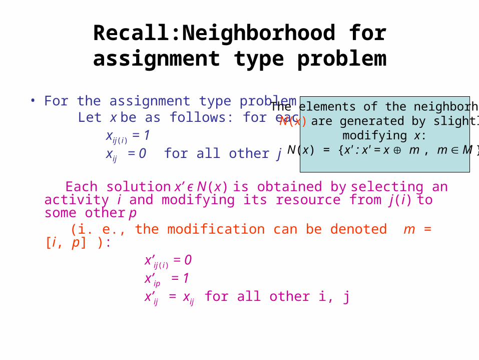
• For the assignment type problem: Let x be as follows: for each 1≤ i ≤ n, xij(i) = 1 xij = 0 for all other j
Each solution x’ є N(x) is obtained by selecting an activity i and modifying its resource from j(i) to some other p
(i. e., the modification can be denoted m = [i, p] ): x’ij(i) = 0 x’ip = 1 x’ij = xij for all other i, j
The elements of the neighborhood N(x) are generated by slightly
modifying x:N(x) = {x' : x' = x m , m M }
Different neighborhood structures
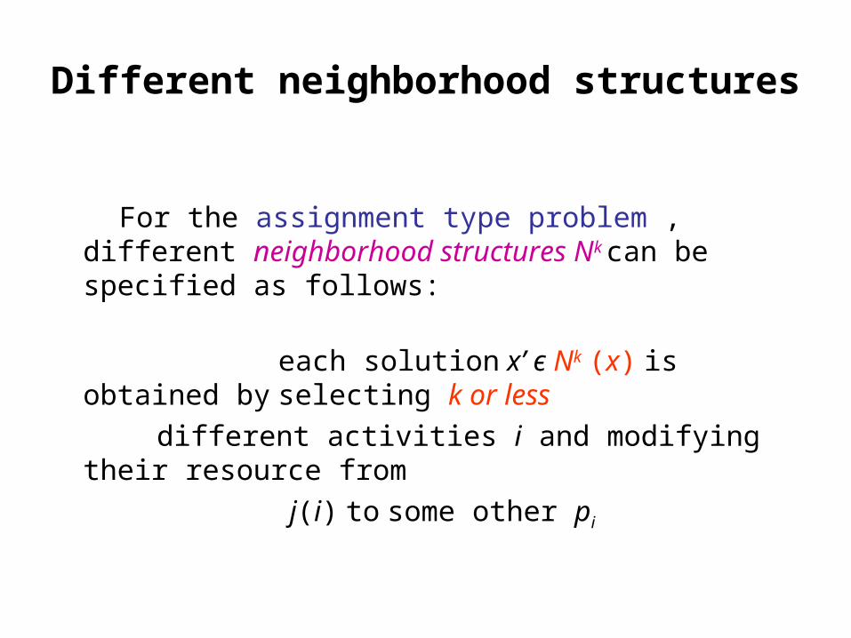
For the assignment type problem , different neighborhood structures Nk can be specified as follows:
each solution x’ є Nk (x) is obtained by selecting k or less
different activities i and modifying their resource from
j(i) to some other pi
Exchange Procedure
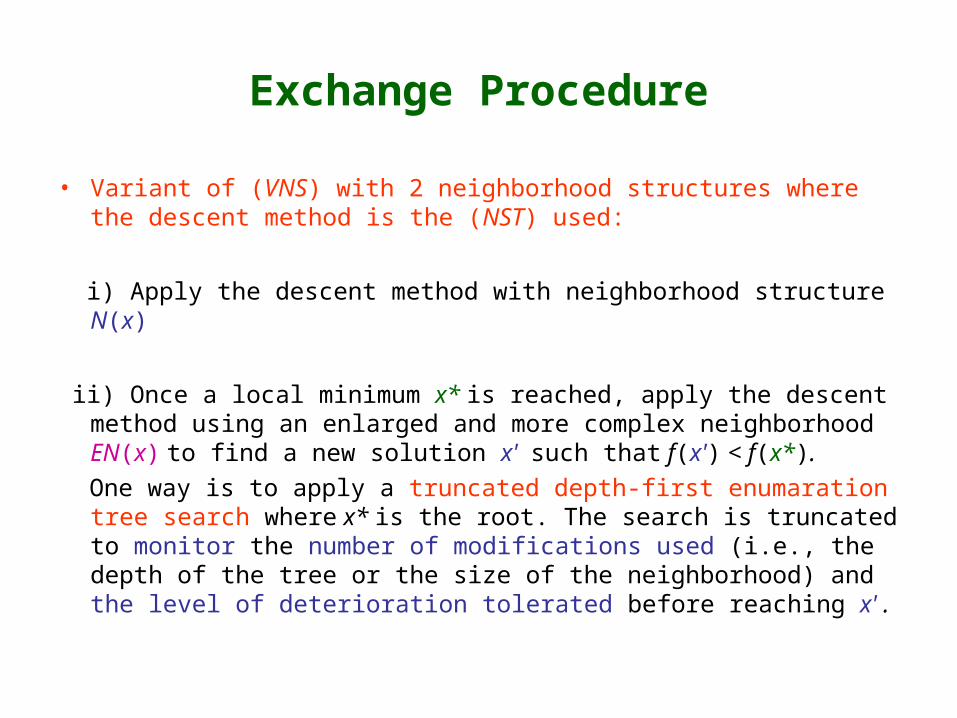
• Variant of (VNS) with 2 neighborhood structures where the descent method is the (NST) used:
i) Apply the descent method with neighborhood structure N(x)
ii) Once a local minimum x* is reached, apply the descent method using an enlarged and more complex neighborhood EN(x) to find a new solution x' such that f(x') < f(x*).
One way is to apply a truncated depth-first enumaration tree search where x* is the root. The search is truncated to monitor the number of modifications used (i.e., the depth of the tree or the size of the neighborhood) and the level of deterioration tolerated before reaching x' .

Material from the following reference
• Jacques A. Ferland and Daniel Costa, “ Heuristic Search Methods for Combinatorial Programming Problems”, Publication # 1193, Dep. I. R. O., Université de Montréal, Montréal, Canada (March 2001)