od metaheuristics 2010
TRANSCRIPT
7/24/2019 OD Metaheuristics 2010
http://slidepdf.com/reader/full/od-metaheuristics-2010 1/57
1
METAHEURISTICS
Introduction
Some problems are so complicated that are not
possible to solve for an optimal solution.
In these problems, it is still important to find a good
feasible solution close to the optimal.
A heuristic method is a procedure to find a very good
feasible solution of a considered problem.
Procedure should be efficient to deal with very large
problems, and is an iterative algorithm .
Heuristic methods usually fit a specific problem rather
than a variety of problems.
409
7/24/2019 OD Metaheuristics 2010
http://slidepdf.com/reader/full/od-metaheuristics-2010 2/57
2
Introduction
For a new problem, OR team would need to start from
scratch to develop a heuristic method.
This changed with the development of metaheuristics.
A metaheuristic is a general solution method that
provides:
a general structure;
guidelines for developing a heuristic method for a
particular type of problem.
410
Nature of metaheuristics
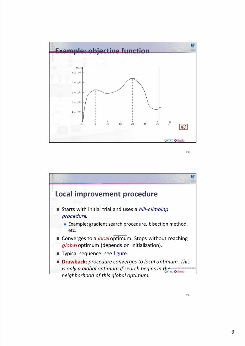
Example: maximize
Function has three local optima. The example is a nonconvex programming problem.
f ( x) is sufficiently complicated to solve analitically.
Simple heuristic method: conduct a local
improvement procedure.
411
5 4 3 2( ) 12 975 28000 345000 1800000 f x x x x x x
subject to 0 31 x
7/24/2019 OD Metaheuristics 2010
http://slidepdf.com/reader/full/od-metaheuristics-2010 3/57
3
Example: objective function
412
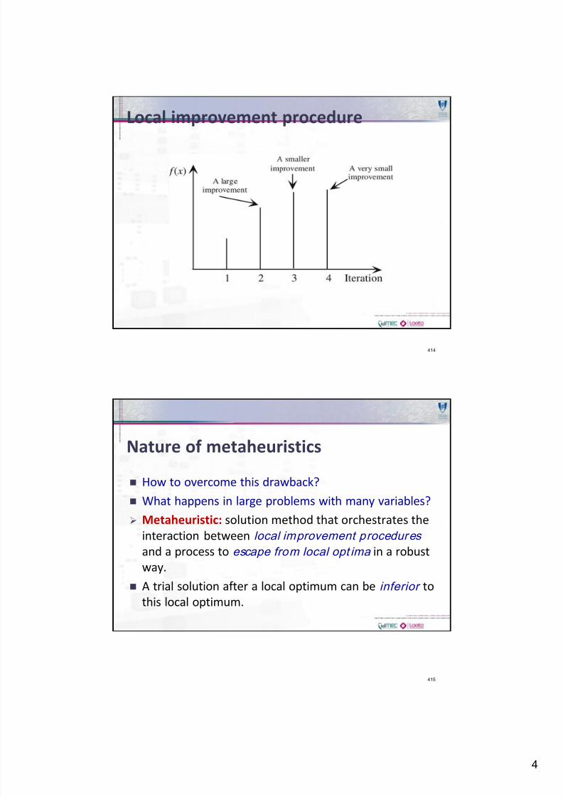
Local improvement procedure
Starts with initial trial and uses a hill-climbing
procedure .
Example: gradient search procedure, bisection method,
etc.
Converges to a local optimum. Stops without reaching
global optimum (depends on initialization).
Typical sequence: see figure.
Drawback: procedure converges to local optimum. This
is only a global optimum if search begins in the
neighborhood of this global optimum.
413
7/24/2019 OD Metaheuristics 2010
http://slidepdf.com/reader/full/od-metaheuristics-2010 4/57
4
Local improvement procedure
414
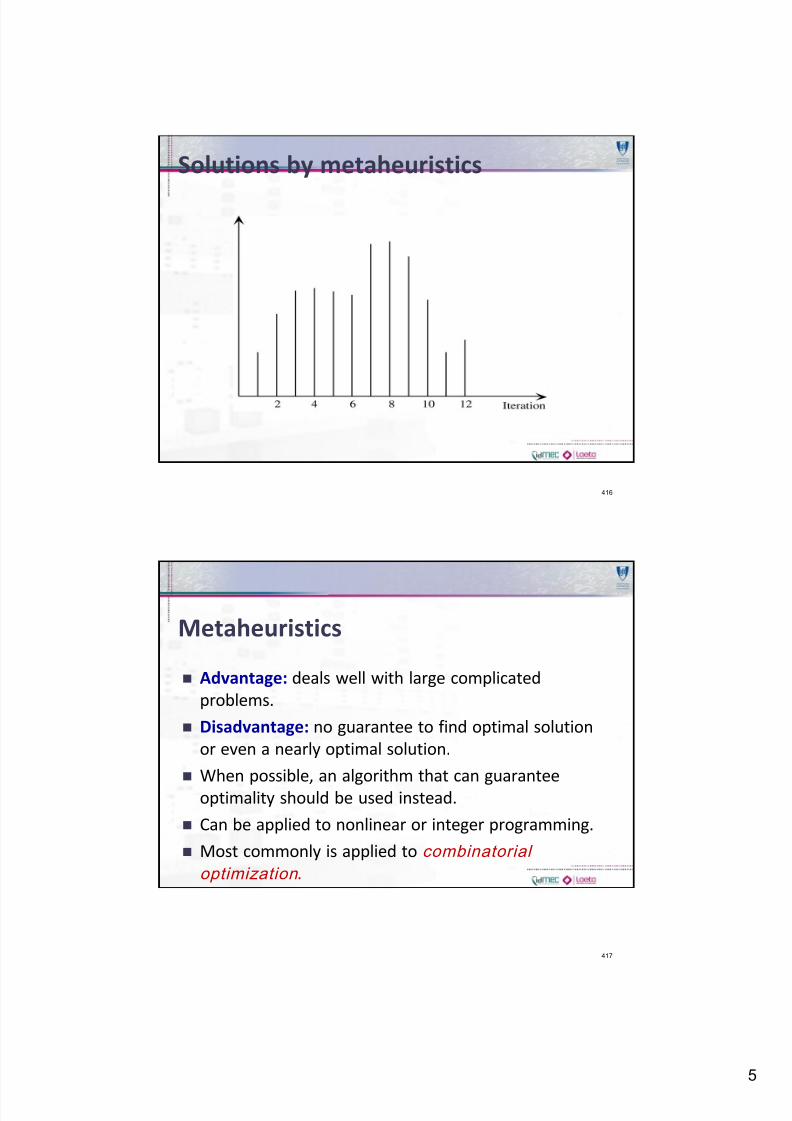
Nature of metaheuristics
How to overcome this drawback?
What happens in large problems with many variables?
Metaheuristic: solution method that orchestrates the
interaction between local improvement procedures
and a process to escape from local opt ima in a robust
way.
A trial solution after a local optimum can be inferior to
this local optimum.
415
7/24/2019 OD Metaheuristics 2010
http://slidepdf.com/reader/full/od-metaheuristics-2010 5/57
5
Solutions by metaheuristics
416
Metaheuristics
Advantage: deals well with large complicated
problems.
Disadvantage: no guarantee to find optimal solution
or even a nearly optimal solution.
When possible, an algorithm that can guarantee
optimality should be used instead.
Can be applied to nonlinear or integer programming.
Most commonly is applied to combinatorial
optimization .
417
7/24/2019 OD Metaheuristics 2010
http://slidepdf.com/reader/full/od-metaheuristics-2010 6/57
6
Most common metaheuristics
Tabu search
Simulated Annealing (SA)
Genetic Algorithms (GA)
Ant Colony Optimization (ACO)
Particle Swarm Optimization (PSO), etc.
418
Common characteristics
Derivat ive freeness : methods rely on evaluations of
objective function; search direction follows heuristic
guidelines.
Intuit ive guidelines : concepts are usually bio-inspired.
Slowness : slower than derivative-based optimization
for continuous optimization problems.
Flexibility : allows any objective function (even
structure of data-fitting model).
419
7/24/2019 OD Metaheuristics 2010
http://slidepdf.com/reader/full/od-metaheuristics-2010 7/57
7
Common characteristics
Randomness : stochastic methods – use random
numbers to determine search directions; may be
“global optimizers” given enough computation time
(optimistic view).
Analytic opacity : knowledge based on empirical
studies due to randomness and problem-specific
nature.
Iterative nature : need of stopping criteria to
determine when to terminate the optimization
process.
420
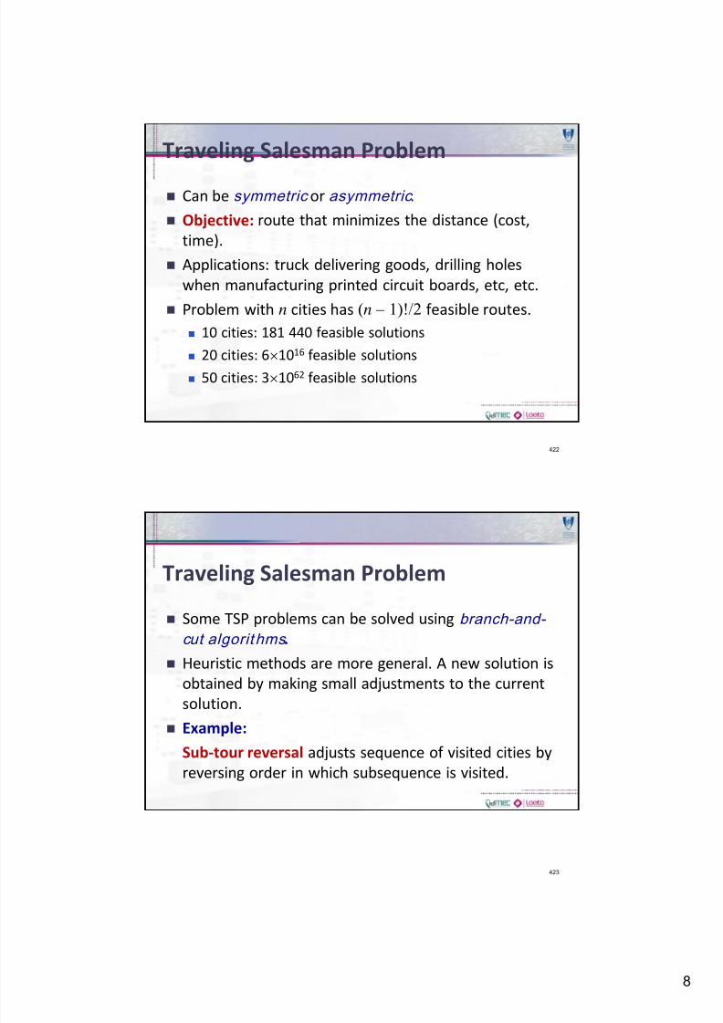
Traveling Salesman Problem
421
7/24/2019 OD Metaheuristics 2010
http://slidepdf.com/reader/full/od-metaheuristics-2010 8/57
8
Traveling Salesman Problem
Can be symmetric or asymmetric .
Objective: route that minimizes the distance (cost,
time).
Applications: truck delivering goods, drilling holes
when manufacturing printed circuit boards, etc, etc.
Problem with n cities has (n – 1)!/2 feasible routes.
10 cities: 181 440 feasible solutions
20 cities: 61016
feasible solutions 50 cities: 31062 feasible solutions
422
Traveling Salesman Problem
Some TSP problems can be solved using branch-and-
cut algorithms .
Heuristic methods are more general. A new solution is
obtained by making small adjustments to the current
solution.
Example:
Sub-tour reversal adjusts sequence of visited cities by
reversing order in which subsequence is visited.
423
7/24/2019 OD Metaheuristics 2010
http://slidepdf.com/reader/full/od-metaheuristics-2010 9/57
9
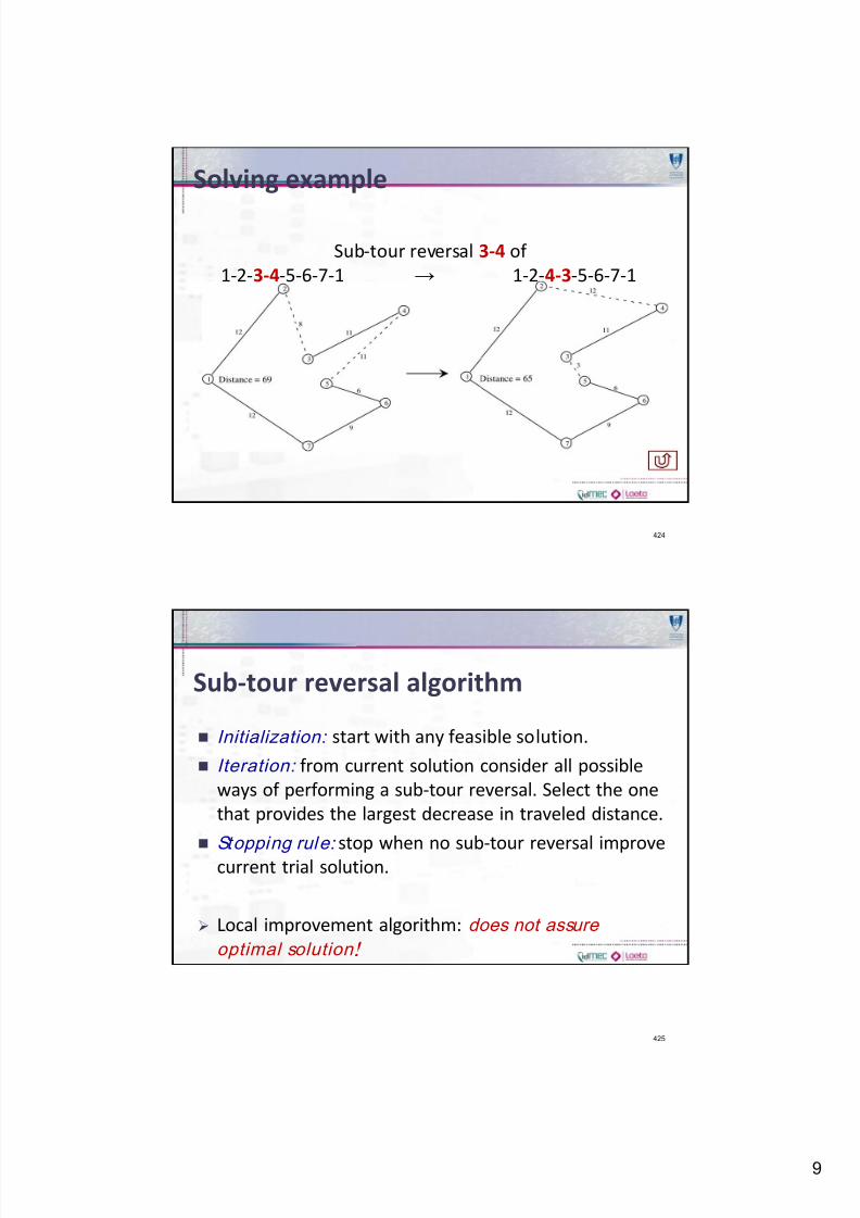
Solving example
424
Sub-tour reversal 3-4 of
1-2-3-4-5-6-7-1 1-2-4-3-5-6-7-1
Sub-tour reversal algorithm
Initialization: start with any feasible solution.
Iteration: from current solution consider all possible
ways of performing a sub-tour reversal. Select the one
that provides the largest decrease in traveled distance.
Stopping rule: stop when no sub-tour reversal improve
current trial solution.
Local improvement algorithm: does not assure
optimal solution!
425
7/24/2019 OD Metaheuristics 2010
http://slidepdf.com/reader/full/od-metaheuristics-2010 10/57
10
Example
Iteration 1: starting with 1-2-3-4-5-6-7-1 (Distance =
69), 4 possible sub-tour reversals that improve
solution are:
Reverse 2-3: 1-3-2-4-5-6-7-1 Distance = 68
Reverse 3-4: 1-2-4-3-5-6-7-1 Distance = 65
Reverse 4-5: 1-2-3-5-4-6-7-1 Distance = 65
Reverse 5-6: 1-2-3-4-6-5-7-1 Distance = 66
426
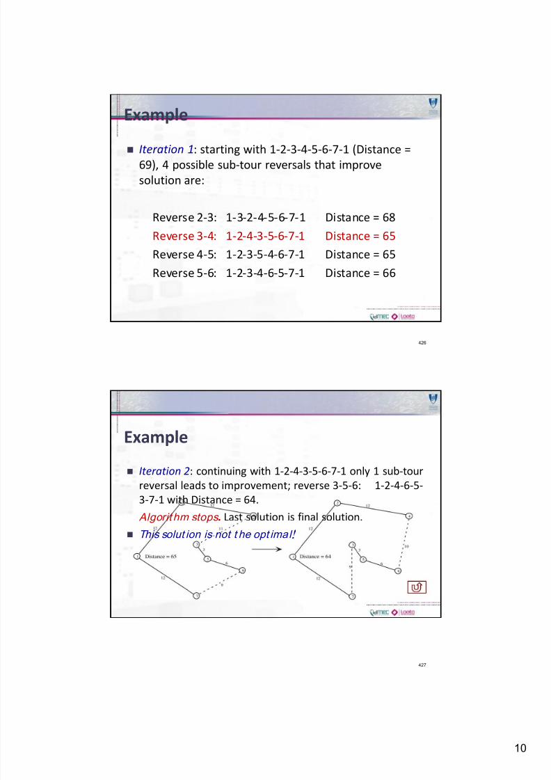
Example
Iteration 2: continuing with 1-2-4-3-5-6-7-1 only 1 sub-tour
reversal leads to improvement; reverse 3-5-6: 1-2-4-6-5-
3-7-1 with Distance = 64.
Algorit hm stops . Last solution is final solution.
This solut ion is not t he opt imal!
427
7/24/2019 OD Metaheuristics 2010
http://slidepdf.com/reader/full/od-metaheuristics-2010 11/57
11
Tabu Search
Fred Glover, 1977
Includes a local search procedure, allowing non-
improvement moves to the best solution.
Referred to as steepest ascent/mildest descent
approach.
To avoid cycle in local optimum, a tabu list is added.
Tabu list records forbidden moves, knows as tabu
moves. Thus, it uses memory to guide the search.
Can include intensification or diversification.
428
Basic tabu search algorithm
Initialization: start with a feasible initial solution.
Iteration:
1. Use local search to define feasible moves in
neighborhood.
2. Eliminates moves in tabu list, unless it results in a
better solution.
3. Determine which move provides best solution.
4. Adopt this solution as next trial solution.
5. Update tabu list.
Stopping rule: stop using fixed number of iterations,
fixed number of iterations without improvement, etc.
429
7/24/2019 OD Metaheuristics 2010
http://slidepdf.com/reader/full/od-metaheuristics-2010 12/57
12
Questions in tabu search
1. Which local search procedure should be used?
2. How to define the neighborhood structure ?
3. How to represent tabu moves in the tabu list?
4. Which tabu list should be added to the tabu list in
each iteration?
5. How long should a tabu move remain in the tabu list?
6. Which stopping rule should be used?
430
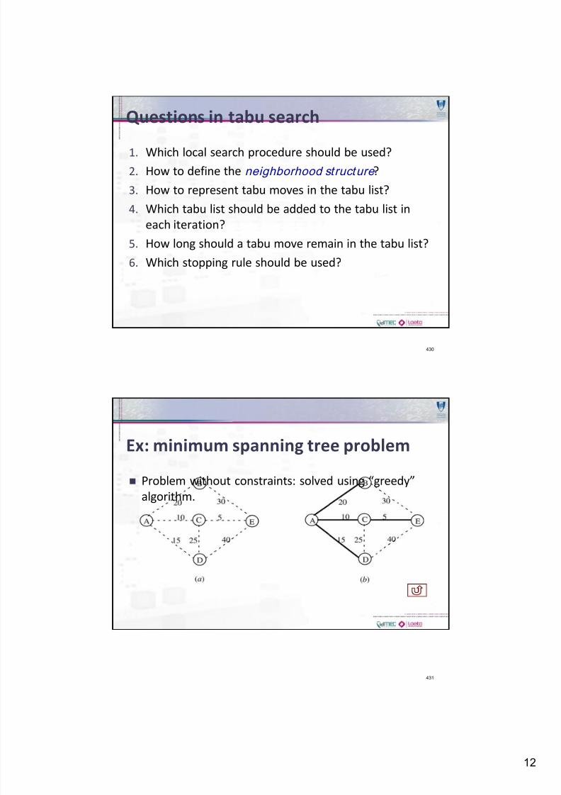
Ex: minimum spanning tree problem
Problem without constraints: solved using “greedy”
algorithm.
431
7/24/2019 OD Metaheuristics 2010
http://slidepdf.com/reader/full/od-metaheuristics-2010 13/57
13
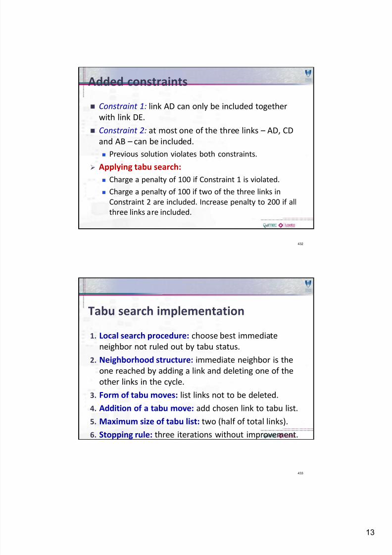
Added constraints
Constraint 1: link AD can only be included together
with link DE.
Constraint 2: at most one of the three links – AD, CD
and AB – can be included.
Previous solution violates both constraints.
Applying tabu search:
Charge a penalty of 100 if Constraint 1 is violated.
Charge a penalty of 100 if two of the three links inConstraint 2 are included. Increase penalty to 200 if all
three links are included.
432
Tabu search implementation
1. Local search procedure: choose best immediate
neighbor not ruled out by tabu status.
2. Neighborhood structure: immediate neighbor is the
one reached by adding a link and deleting one of the
other links in the cycle.
3. Form of tabu moves: list links not to be deleted.
4. Addition of a tabu move: add chosen link to tabu list.
5. Maximum size of tabu list: two (half of total links).
6. Stopping rule: three iterations without improvement.
433
7/24/2019 OD Metaheuristics 2010
http://slidepdf.com/reader/full/od-metaheuristics-2010 14/57
14
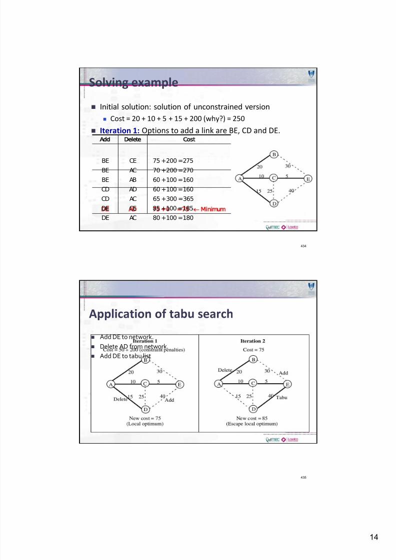
Solving example
Initial solution: solution of unconstrained version
Cost = 20 + 10 + 5 + 15 + 200 (why?) = 250
Iteration 1: Options to add a link are BE, CD and DE.
434
Add Delete Cost
BE CE 75 +200 =275
BE AC 70 +200 =270
BE AB 60 +100 =160
CD AD 60 +100 =160
CD AC 65 +300 =365
DE CE 85 +100 =185
DE AC 80 +100 =180
DE AD 75 + 0 = 75 Minimum
Application of tabu search
Add DE to network.
Delete AD from network.
Add DE to tabu list
435
7/24/2019 OD Metaheuristics 2010
http://slidepdf.com/reader/full/od-metaheuristics-2010 15/57
15
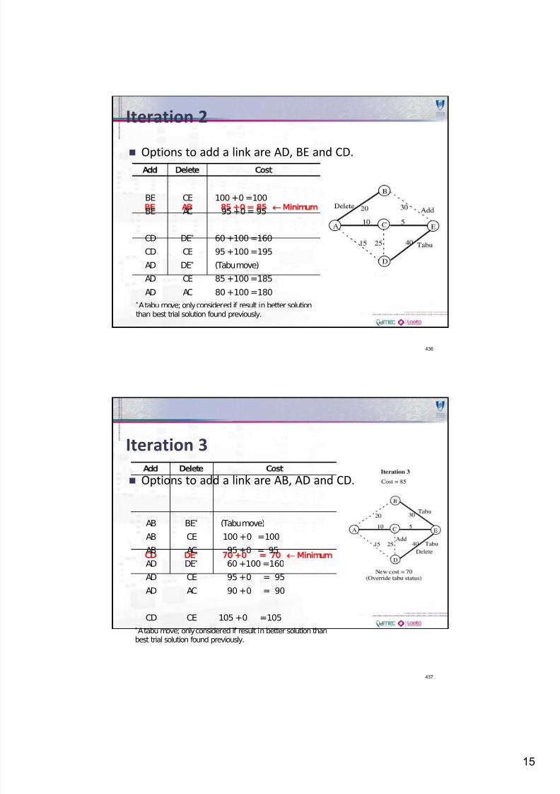
Iteration 2
Options to add a link are AD, BE and CD.
436
Add Delete Cost
BE CE 100 +0 =100
BE AC 95 +0 = 95
BE AB 85 + 0 = 85
Minimum
CD DE* 60 +100 =160
CD CE 95 +100 =195
AD DE* (Tabu move)
AD CE 85 +100 =185
AD AC 80 +100 =180*A tabu move; only considered if result in better solutionthan best trial solution found previously.
Iteration 3
Options to add a link are AB, AD and CD.
437
Add Delete Cost
AB BE* (Tabu move)
AB CE 100 +0 =100
AB AC 95 +0 = 95
AD DE* 60 +100 =160
AD CE 95 +0 = 95
AD AC 90 +0 = 90
CD DE
70 + 0 = 70
Minimum
CD CE 105 +0 =105
*A tabu move; only considered if result in better solution thanbest trial solution found previously.
7/24/2019 OD Metaheuristics 2010
http://slidepdf.com/reader/full/od-metaheuristics-2010 16/57
16
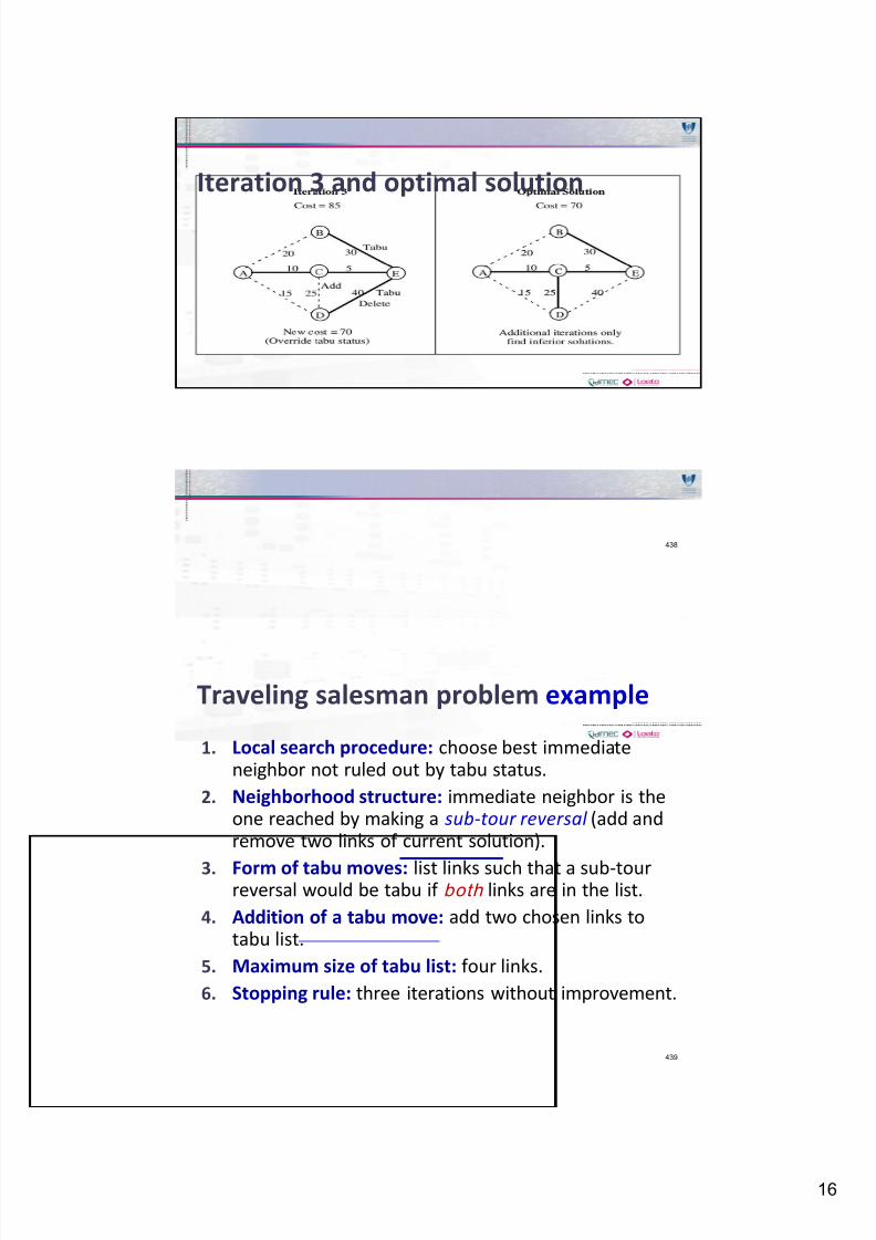
Iteration 3 and optimal solution
438
Traveling salesman problem example
1. Local search procedure: choose best immediateneighbor not ruled out by tabu status.
2. Neighborhood structure: immediate neighbor is theone reached by making a sub-tour reversal (add andremove two links of current solution).
3. Form of tabu moves: list links such that a sub-tourreversal would be tabu if both links are in the list.
4. Addition of a tabu move: add two chosen links totabu list.
5. Maximum size of tabu list: four links.
6. Stopping rule: three iterations without improvement.
439
7/24/2019 OD Metaheuristics 2010
http://slidepdf.com/reader/full/od-metaheuristics-2010 17/57
17
Solving problem
Init ial t rial solution: 1-2-3-4-5-6-7-1 Distance = 69
Iterat ion 1: choose to reverse 3-4.
Deleted links: 2-3 and 4-5
Added links (tabu list): 2-4 and 3-5
New trial solution: 1-2-4-3-5-6-7-1 Distance = 65
Iterat ion 2: choose to reverse 3-5-6.
Deleted links: 4-3 and 6-7 (OK since not in tabu list)
Added links: 4-6 and 3-7 Tabu list: 2-4, 3-5, 4-6 and 3-7
New trial solution: 1-2-4-6-5-3-7-1 Distance = 64
440
Solving problem
Only two immediate neighbors:
Reverse 6-5-3: 1-2-4-3-5-6-7-1 Distance = 65. (This
would delete links 4-6 and 3-7 that are in the tabu list.)
Reverse 3-7: 1-2-4-6-5-7-3-1 Distance = 66
Iterat ion 3: choose to reverse 3-7.
Deleted links: 5-3 and 7-1
Added links: 5-7 and 3-1
Tabu list: 4-6, 3-7, 5-7 and 3-1
New trial solution: 1-2-4-6-5-7-3-1 Distance = 66
441
7/24/2019 OD Metaheuristics 2010
http://slidepdf.com/reader/full/od-metaheuristics-2010 18/57
18
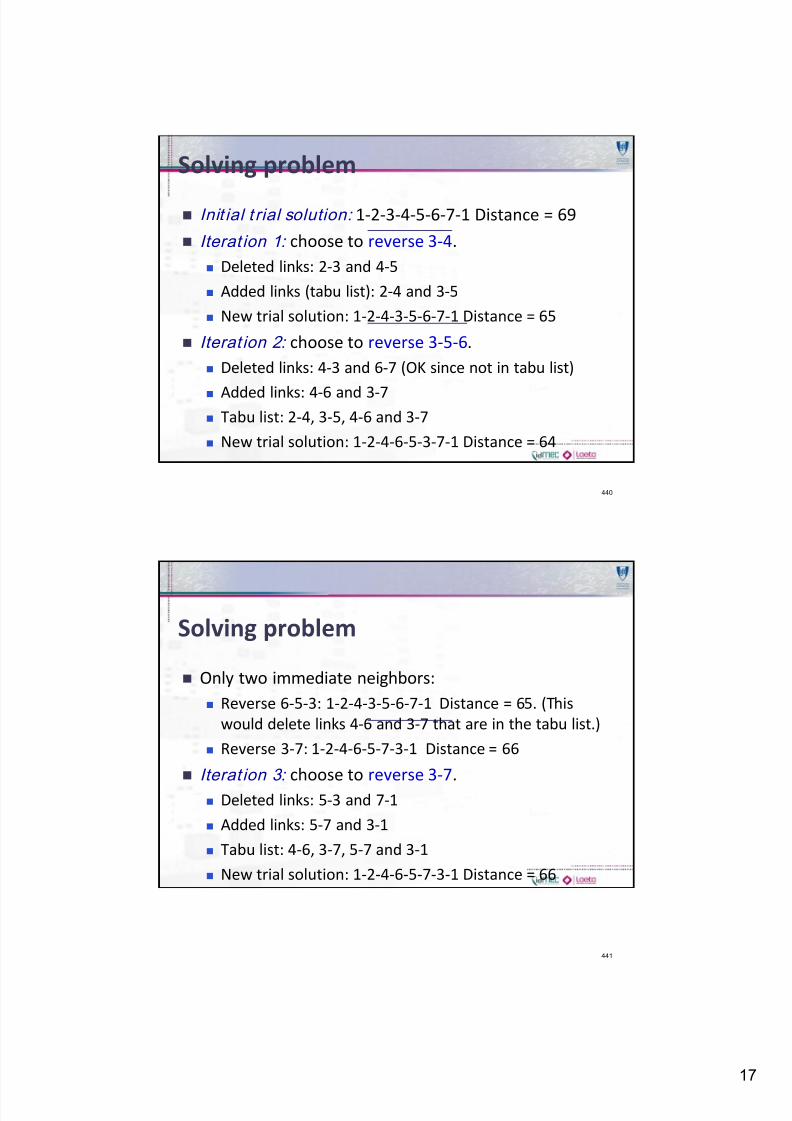
Sub-tour reversal of 3-7 (Iteration 3)
442
Iteration 4
Four immediate neighbors:
Reverse 2-4-6-5-7: 1-7-5-6-4-2-3-1 Distance = 65
Reverse 6-5: 1-2-4-5-6-7-3-1 Distance = 69
Reverse 5-7: 1-2-4-6-7-5-3-1 Distance = 63
Reverse 7-3: 1-2-4-5-6-3-7-1 Distance = 64 Iterat ion 4: choose to reverse 5-7.
Deleted links: 6-5 and 7-3
Added links: 6-7 and 5-3
Tabu list: 5-7, 3-1, 6-7 and 5-3
New trial (final) solution: 1-2-4-6-7-5-3-1 Distance = 63
443
7/24/2019 OD Metaheuristics 2010
http://slidepdf.com/reader/full/od-metaheuristics-2010 19/57
19
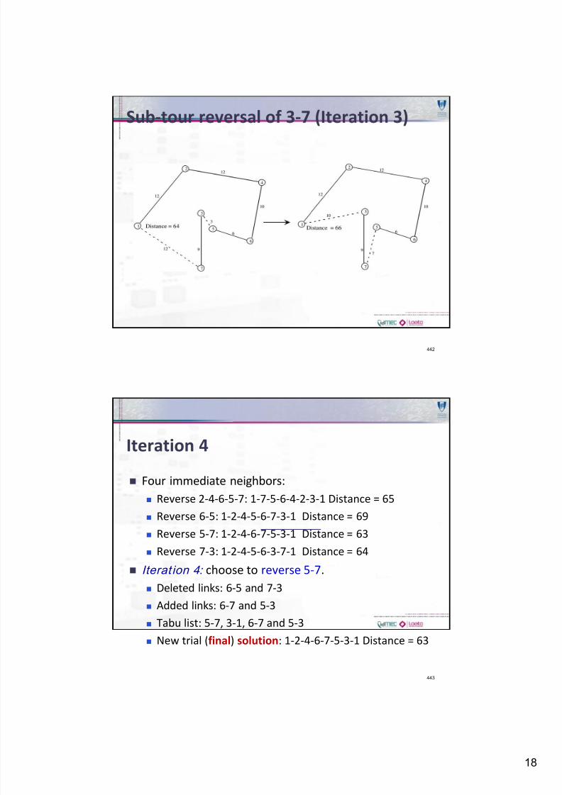
Sub-tour reversal of 5-7 (Iteration 4)
444
Simulated Annealing
Kirkpatrick, Gelatt, Vecchi, 1983
Suitable for continuous and discrete optimization
problems.
Effective in finding near optimal solutions for large-
scale combinatorial problems such as TSP.
Enables search process to escape from local minima.
Instead of steepest ascent/mildest descent approach
as in tabu search, it tries to search for the tallest hill.
Early iterations take steps in random directions.
445
7/24/2019 OD Metaheuristics 2010
http://slidepdf.com/reader/full/od-metaheuristics-2010 20/57
20
Simulated Annealing
Principle analogous to metals behavior when cooled at
a controlled rate.
Value of objective function analogous to energy in
thermodynamic systems:
At high temperatures, it is likely to accept a new point
with higher energy.
At low temperatures, likelihood of accepting a new
point with higher energy is much lower.
Annealing or cooling schedule : specifies how rapidly
the temperature is lowered from high to low values.
446
Simulated Annealing
Let
Z c = objective function value for current trial solution.
Z n = objective function value for candidate of next trial
solution.
T = tendency to accept Z n if not better than currentsolution.
447
7/24/2019 OD Metaheuristics 2010
http://slidepdf.com/reader/full/od-metaheuristics-2010 21/57
21
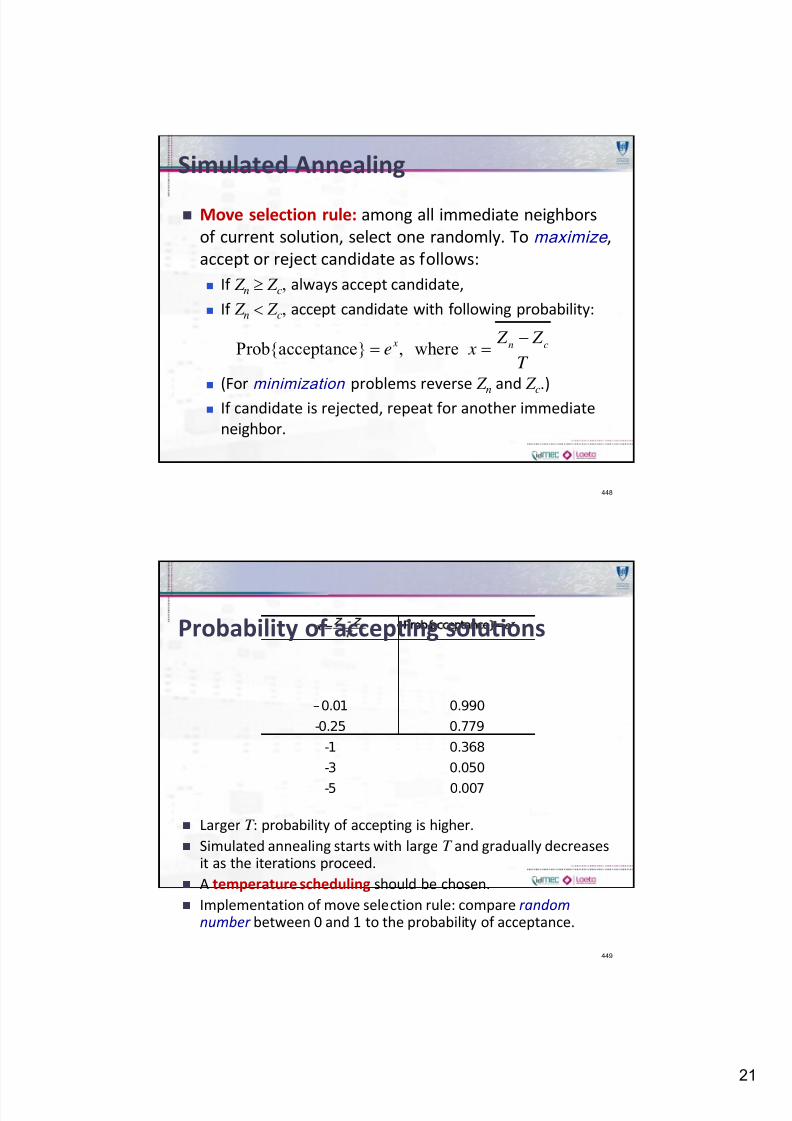
Simulated Annealing
Move selection rule: among all immediate neighbors
of current solution, select one randomly. To maximize ,
accept or reject candidate as follows:
If Z n Z c, always accept candidate,
If Z n Z c, accept candidate with following probability:
(For minimization problems reverse Z n
and Z c.)
If candidate is rejected, repeat for another immediate
neighbor.
448
Prob{acceptance} , where x n c
Z Z e x
T
Probability of accepting solutions
Larger T : probability of accepting is higher.
Simulated annealing starts with large T and gradually decreasesit as the iterations proceed.
A temperature scheduling should be chosen.
Implementation of move selection rule: compare randomnumber between 0 and 1 to the probability of acceptance.
449
Prob{acceptance}=
–0.01 0.990
-0.25 0.779
-1 0.368
-3 0.050
-5 0.007
n c
Z
x
T
7/24/2019 OD Metaheuristics 2010
http://slidepdf.com/reader/full/od-metaheuristics-2010 22/57
22
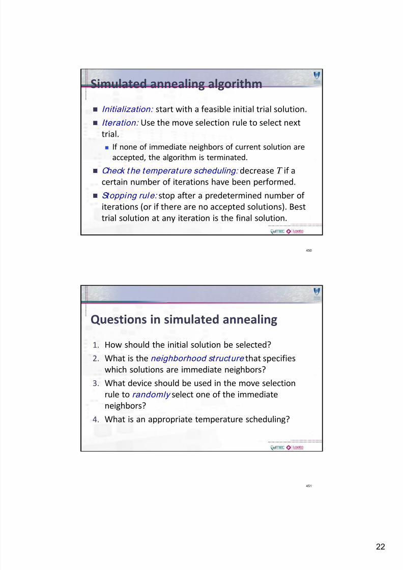
Simulated annealing algorithm
Initialization: start with a feasible initial trial solution.
Iteration: Use the move selection rule to select next
trial.
If none of immediate neighbors of current solution are
accepted, the algorithm is terminated.
Check t he temperature scheduling: decrease T if a
certain number of iterations have been performed.
Stopping rule: stop after a predetermined number of iterations (or if there are no accepted solutions). Best
trial solution at any iteration is the final solution.
450
Questions in simulated annealing
1. How should the initial solution be selected?
2. What is the neighborhood structure that specifies
which solutions are immediate neighbors?
3. What device should be used in the move selection
rule to randomly select one of the immediate
neighbors?
4. What is an appropriate temperature scheduling?
451
7/24/2019 OD Metaheuristics 2010
http://slidepdf.com/reader/full/od-metaheuristics-2010 23/57
23
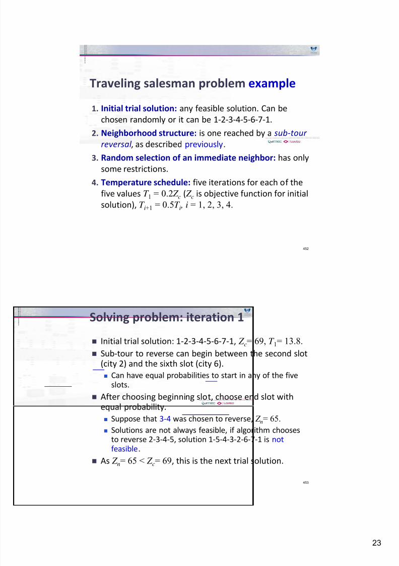
Traveling salesman problem example
1. Initial trial solution: any feasible solution. Can be
chosen randomly or it can be 1-2-3-4-5-6-7-1.
2. Neighborhood structure: is one reached by a sub-tour
reversal , as described previously.
3. Random selection of an immediate neighbor: has only
some restrictions.
4. Temperature schedule: five iterations for each of the
five values T 1 = 0.2 Z c
( Z c
is objective function for initial
solution), T i+1 = 0.5T i , i = 1, 2, 3, 4.
452
Solving problem: iteration 1
Initial trial solution: 1-2-3-4-5-6-7-1, Z c= 69, T 1= 13.8.
Sub-tour to reverse can begin between the second slot(city 2) and the sixth slot (city 6).
Can have equal probabilities to start in any of the fiveslots.
After choosing beginning slot, choose end slot withequal probability.
Suppose that 3-4 was chosen to reverse, Z n= 65.
Solutions are not always feasible, if algorithm choosesto reverse 2-3-4-5, solution 1-5-4-3-2-6-7-1 is notfeasible.
As Z n= 65 < Z c= 69, this is the next trial solution.
453
7/24/2019 OD Metaheuristics 2010
http://slidepdf.com/reader/full/od-metaheuristics-2010 24/57
24
Solving problem
Suppose that Iteration 2 results in reversing 3-5-6, to
obtain 1-2-4-6-5-3-7-1, with Z n= 64.
Suppose now that Iteration 3 results in reversing 3-7,
to obtain 1-2-4-6-5-7-3-1, with Z n= 66. As Z n > Z c:
One application of SA gave best solution 1-3-5-7-6-4-2-1
at iterations 13 and 15 (out of 25) with distance = 63.
454
2/13.8
Prob{acceptance}
0.865
n c Z Z
T e
e
Nonlinear programming application
Problems of the type:
1. Initial trial solution: any feasible solution. Can be
x j = L j + (U j – L j)/2.
2. Neighborhood structure: any feasible solution, see
random selection of immediate neighbor.
455
1Maximize ( , , ) n f x x
subject to
, for 1, ,
j j j L x U j n
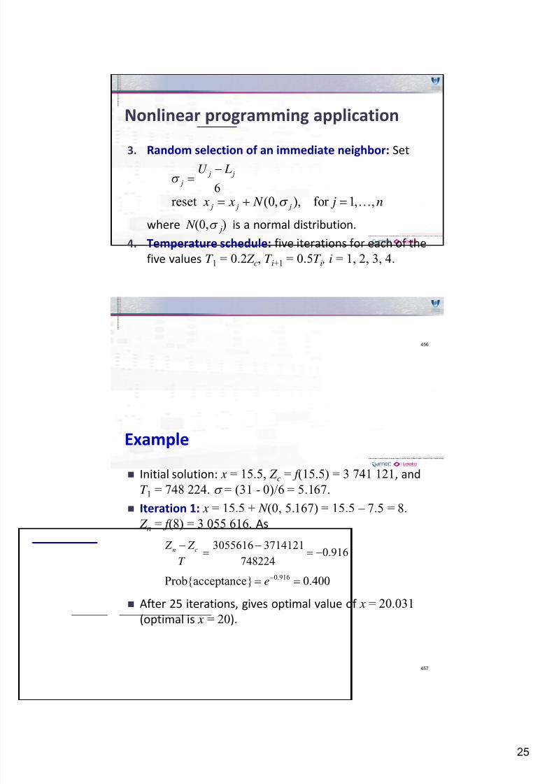
7/24/2019 OD Metaheuristics 2010
http://slidepdf.com/reader/full/od-metaheuristics-2010 25/57
25
Nonlinear programming application
3. Random selection of an immediate neighbor: Set
where N (0, j) is a normal distribution.
4. Temperature schedule: five iterations for each of the
five values T 1 = 0.2 Z c, T i+1 = 0.5T i , i = 1, 2, 3, 4.
456
6
j j
j
U L
reset (0, ), for 1, , j j j x x N j n
Example
Initial solution: x = 15.5, Z c = f (15.5) = 3 741 121, and
T 1 = 748 224. = (31 - 0)/6 = 5.167.
Iteration 1: x = 15.5 + N (0, 5.167) = 15.5 – 7.5 = 8.
Z n = f (8) = 3 055 616. As
After 25 iterations, gives optimal value of x = 20.031
(optimal is x = 20).
457
3055616 3714121 0.916748224 n c Z Z
T
0.916Prob{acceptance} 0.400 e
7/24/2019 OD Metaheuristics 2010
http://slidepdf.com/reader/full/od-metaheuristics-2010 26/57
26
GENETICALGORITHMS
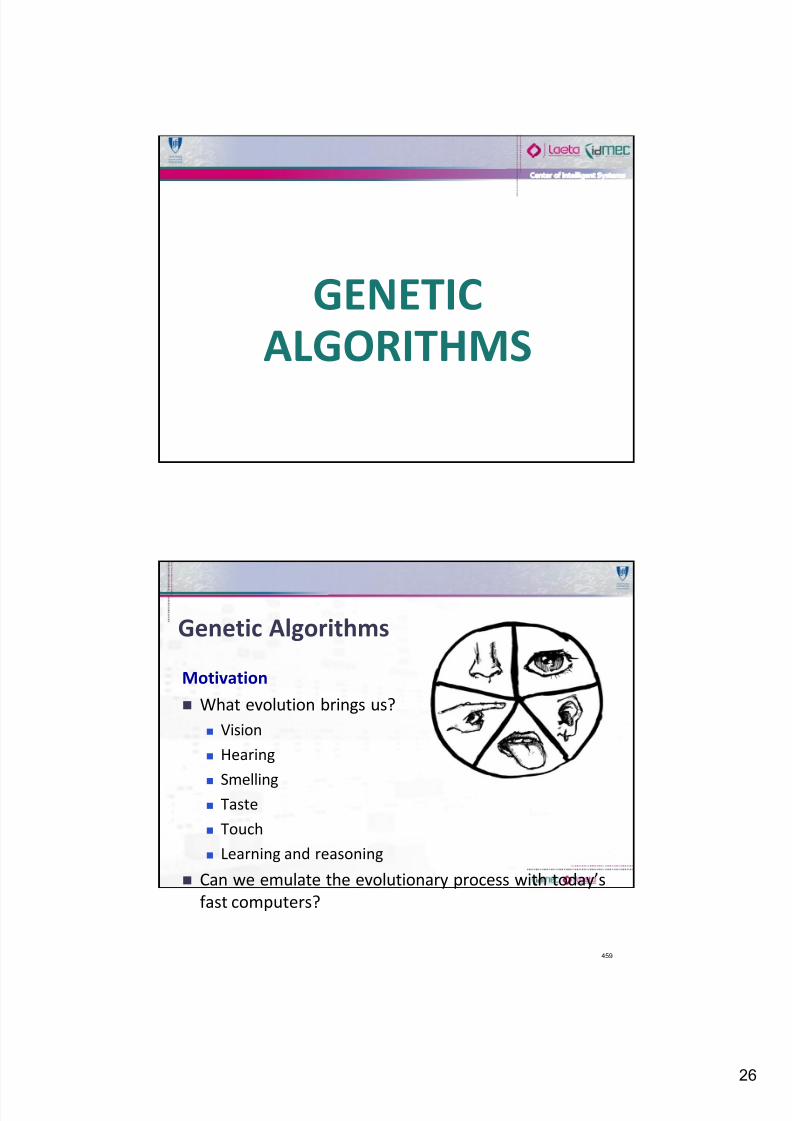
Genetic Algorithms
Motivation
What evolution brings us?
Vision
Hearing
Smelling Taste
Touch
Learning and reasoning
Can we emulate the evolutionary process with today’s
fast computers?
459
7/24/2019 OD Metaheuristics 2010
http://slidepdf.com/reader/full/od-metaheuristics-2010 27/57
27
Genetic Algorithms
Introduced by John Holland in 1975.
Randomized search algorithms based on mechanics of
natural selection and genetics.
Principle of natural selection through ‘survival of the
fittest’ with randomized search.
Search efficiently in large spaces.
Robust with respect to the complexity of the search
problem. Use a population of solutions instead of searching only
one solution at a time: easily parallelized algorithms.
460
Basic elements
Candidate solut ion is encoded as a string of characters
in binary or real. Bit string is called a chromosome.
Solution represented by a chromosome is the
individual . A number of individuals form a population.
Population is updated iteratively; each iteration is
called a generation.
Objective function is called the fitness function.
Fitness value is maximized.
Multiple solutions are evaluated in parallel.
461
7/24/2019 OD Metaheuristics 2010
http://slidepdf.com/reader/full/od-metaheuristics-2010 28/57
28
Definitions
Population: a collection of solutions for the studied
(optimization) problem.
Individual: a single solution in a GA.
Chromosome: (bit string) representation of a single
solution.
Gene: part of a chromosome, usually representing a
variable characterizing part of the solution.
462
Definitions
Encoding: conversion of a solution to its equivalent bit
string representation (chromosome).
Decoding: conversion of a chromosome to its
equivalent solution.
Fitness: scalar value denoting the suitability of a
solution.
463
7/24/2019 OD Metaheuristics 2010
http://slidepdf.com/reader/full/od-metaheuristics-2010 29/57
29
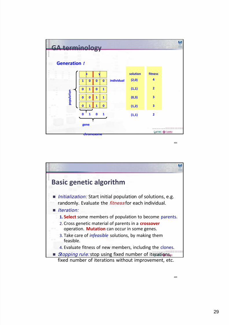
GA terminology
464
1 0 0 0
0 0 1 1
0 1 1 0
0 1 0 1
0 1 0 1
p o p u l a t i o n
x y
gene
chromosome
individual
solution fitness
(2,0)
(1,1)
(0,3)
(1,2)
(1,1)
4
2
3
3
2
Generation t
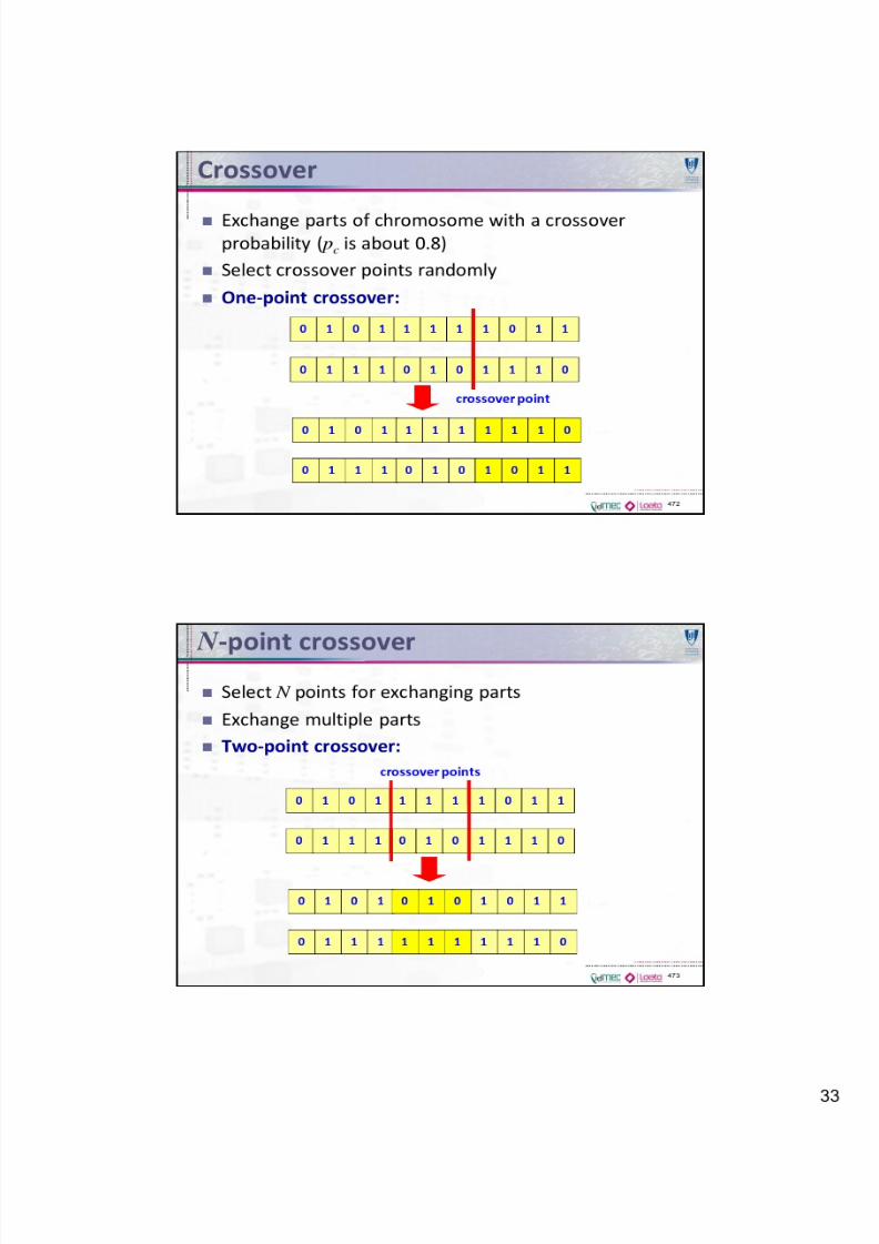
Basic genetic algorithm
Initialization : Start initial population of solutions, e.g.
randomly. Evaluate the fitness for each individual.
Iteration:
1. Select some members of population to become parents.
2. Cross genetic material of parents in a crossover
operation. Mutation can occur in some genes.
3. Take care of infeasible solutions, by making themfeasible.
4. Evaluate fitness of new members, including the clones.
Stopping rule: stop using fixed number of iterations,fixed number of iterations without improvement, etc.
465
7/24/2019 OD Metaheuristics 2010
http://slidepdf.com/reader/full/od-metaheuristics-2010 30/57
30
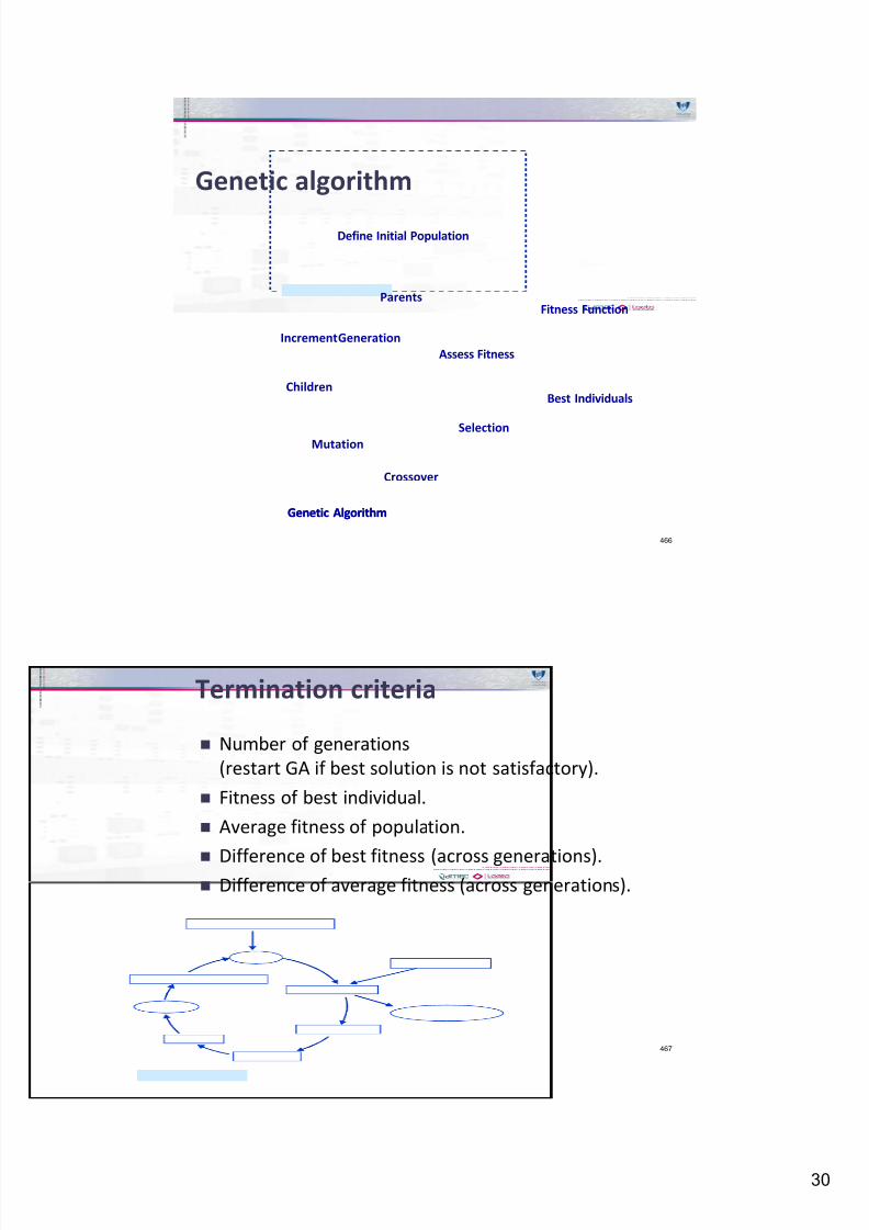
Genetic algorithm
466
Genetic AlgorithmGenetic Algorithm
Fitness Function
Assess Fitness
Selection
Crossover
Mutation
Increment Generation
Define Initial Population
Parents
Best IndividualsChildren
Termination criteria
Number of generations
(restart GA if best solution is not satisfactory).
Fitness of best individual.
Average fitness of population.
Difference of best fitness (across generations). Difference of average fitness (across generations).
467
7/24/2019 OD Metaheuristics 2010
http://slidepdf.com/reader/full/od-metaheuristics-2010 31/57
31
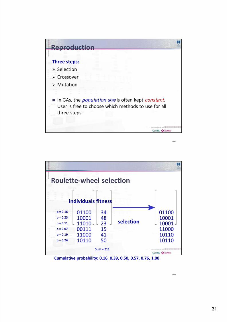
Reproduction
Three steps:
Selection
Crossover
Mutation
In GAs, the populat ion size is often kept constant .
User is free to choose which methods to use for all
three steps.
468
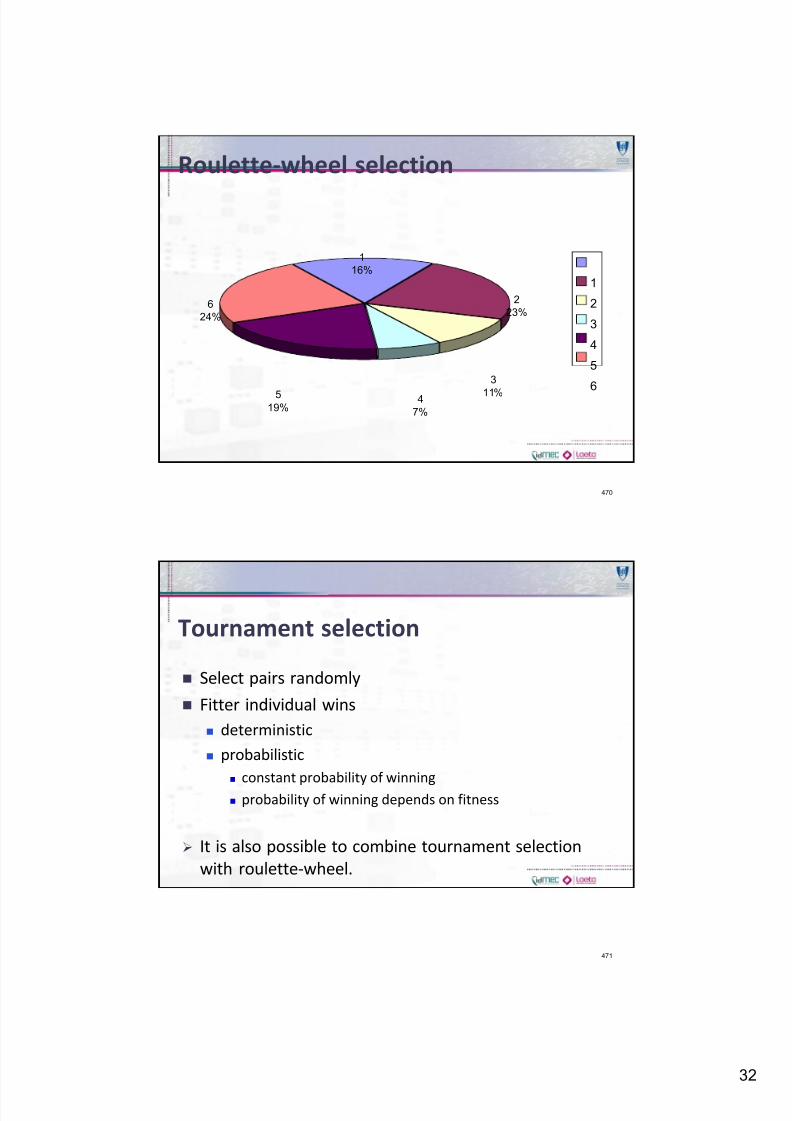
Roulette-wheel selection
469
0110010001
11010001111100010110
0110010001
10001110001011010110
3448
23154150
selection
fitnessindividuals
Sum = 211
p = 0.16
p = 0.23
p = 0.11
p = 0.07
p = 0.19
p = 0.24
Cumulative probability: 0.16, 0.39, 0.50, 0.57, 0.76, 1.00
7/24/2019 OD Metaheuristics 2010
http://slidepdf.com/reader/full/od-metaheuristics-2010 32/57
32
Roulette-wheel selection
470
1
16%
2
23%
3
11%4
7%
5
19%
6
24%
1
2
3
4
5
6
Tournament selection
Select pairs randomly
Fitter individual wins
deterministic
probabilistic
constant probability of winning
probability of winning depends on fitness
It is also possible to combine tournament selection
with roulette-wheel.
471
7/24/2019 OD Metaheuristics 2010
http://slidepdf.com/reader/full/od-metaheuristics-2010 33/57
7/24/2019 OD Metaheuristics 2010
http://slidepdf.com/reader/full/od-metaheuristics-2010 34/57
7/24/2019 OD Metaheuristics 2010
http://slidepdf.com/reader/full/od-metaheuristics-2010 35/57
35
GA iteration
476
10010110
01100010
10100100
10011001
01111101
. . .
. . .
. . .
10010110
01100010
10100100
10011101
01111001
. . .
. . .
. . .
Selection Crossover Mutation
Current
generation
Next
generation
Elitism
reproduction
Spaces in GA iteration
477
0110010001110100011111000
10110
010111011111001000111101001010
1217267
24
22
3448231541
50
genetic-operators
(de)coding fitness functiongeneration N
generation N+1
gene-space problem-space fitness-space
fitness operators
7/24/2019 OD Metaheuristics 2010
http://slidepdf.com/reader/full/od-metaheuristics-2010 36/57
36
Encoding and decoding
Chromosomes represent solutions for a problem in a
selected encoding.
Solutions must be encoded into their chromosome
representation and chromosomes must be decoded to
evaluate their fitness.
Success of a GA can depend on the coding used.
May change the nature of the problem.
Common coding methods: simple binary coding
gray coding (binary)
real valued coding (requires special genetic operators)
478
Handling constraints
Explicit: in the fitness function
penalty function
barrier function
setting fitness of unfeasible solutions to zero
(search may be very inefficient due to unfeasible
solutions)
Implicit: (preferred method) with special encoding
GA searches always for feasible solutions
smaller search space
adhoc method, may be difficult to find
479
7/24/2019 OD Metaheuristics 2010
http://slidepdf.com/reader/full/od-metaheuristics-2010 37/57
37
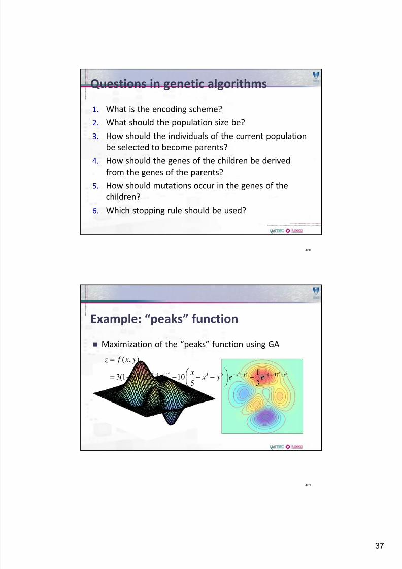
Questions in genetic algorithms
1. What is the encoding scheme?
2. What should the population size be?
3. How should the individuals of the current population
be selected to become parents?
4. How should the genes of the children be derived
from the genes of the parents?
5. How should mutations occur in the genes of the
children?6. Which stopping rule should be used?
480
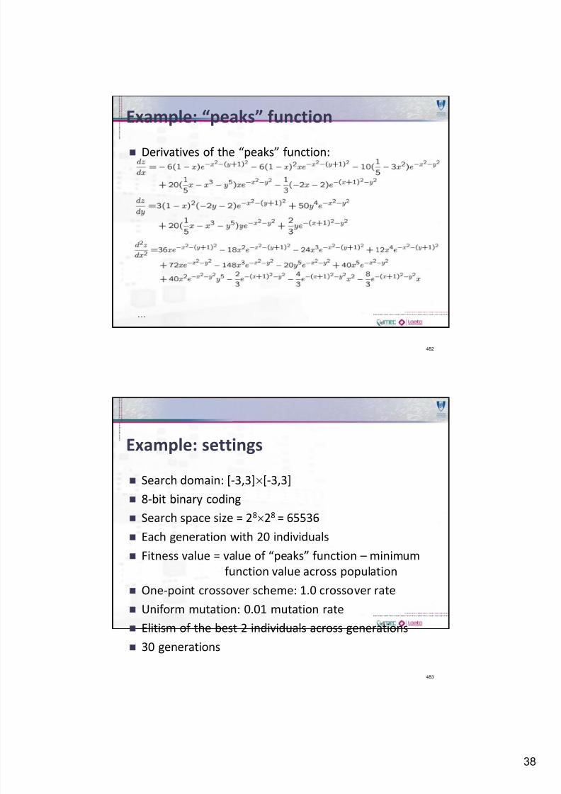
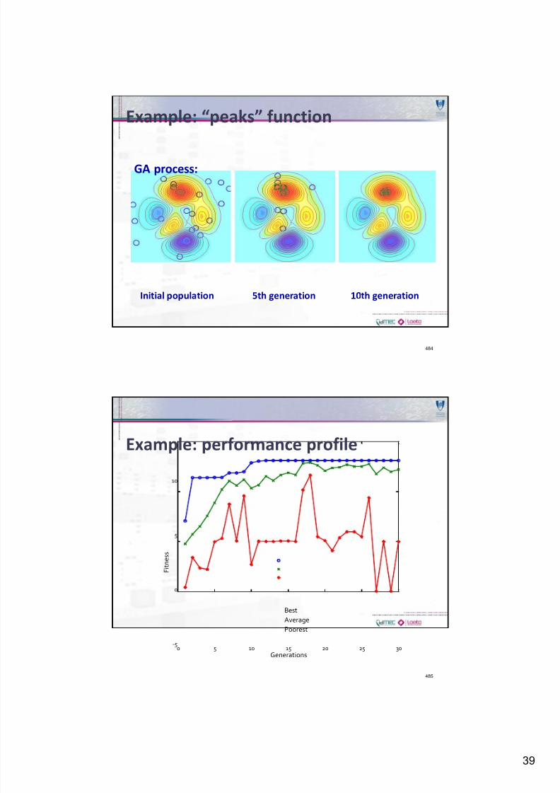
Example: “peaks” function
Maximization of the “peaks” function using GA
481
2 2 2 2 2 22 ( 1) 3 5 ( 1)
( , )
13(1 ) 10
5 3
x y x y x y
z f x y
x x e x y e e
7/24/2019 OD Metaheuristics 2010
http://slidepdf.com/reader/full/od-metaheuristics-2010 38/57
38
Example: “peaks” function
Derivatives of the “peaks” function:
482
…
Example: settings
Search domain: [-3,3][-3,3]
8-bit binary coding
Search space size = 2828 = 65536
Each generation with 20 individuals
Fitness value = value of “peaks” function – minimumfunction value across population
One-point crossover scheme: 1.0 crossover rate
Uniform mutation: 0.01 mutation rate
Elitism of the best 2 individuals across generations
30 generations
483
7/24/2019 OD Metaheuristics 2010
http://slidepdf.com/reader/full/od-metaheuristics-2010 39/57
39
Example: “peaks” function
484
Initial population 5th generation 10th generation
GA process:
Example: performance profile
485
0 5 10 15 20 25 30-5
0
5
10
Generations
F i t n e s
s
Best
Average
Poorest
7/24/2019 OD Metaheuristics 2010
http://slidepdf.com/reader/full/od-metaheuristics-2010 40/57
40
Nonlinear programming example
1. Encoding scheme: integers from 0 to 31. Five binary
genes are needed.
Example: x = 21 is 10101 in base 2.
Note that no infeasible solutions are possible.
2. Population size: 10 (problem is simple).
3. Selection of parents: select randomly 4 from the 5
most fit, and 4 from the 5 least fitted.
Select 3 pairs of parents, that will produce 6 children. Elitism: four best solutions are clones in next
generation.
486
Nonlinear programming example
4. Crossover operator: When a bit is difference in the
two parents, select 0 or 1 randomly (uniform dist.)
Parents are 0x01x. Children can be 01011 and 00010.
5. Mutation operator: mutation rate is 0.1 for each
gene.
6. Stopping criteria: stop after 5 consecutive
generations without improvement.
Fit ness value is just the objective function value in
this example.
6 generations were enough in this example.
487
7/24/2019 OD Metaheuristics 2010
http://slidepdf.com/reader/full/od-metaheuristics-2010 41/57
41
Traveling salesman problem example
1. Encoding scheme: exactly as before.
Example: 1-2-3-4-5-6-7-1.
Initial population: generated randomly, using possible
links between cities.
2. Population size: 10 (problem is simple).
3. Selection of parents: select randomly 4 from the 5
most fit, and 4 from the 5 least fitted.
Select 3 pairs of parents, that will produce 6 children. Elitism: four best solutions are clones in next
generation.
488
Traveling salesman problem example
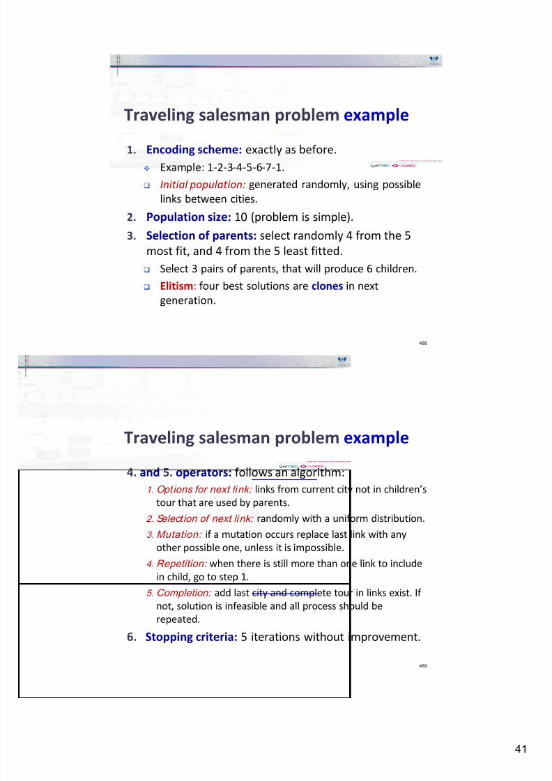
4. and 5. operators: follows an algorithm:
1. Options for next link: links from current city not in children’s
tour that are used by parents.
2. Select ion of next link: randomly with a uniform distribution.
3. Mutation: if a mutation occurs replace last link with any
other possible one, unless it is impossible.4. Repetition: when there is still more than one link to include
in child, go to step 1.
5. Completion: add last city and complete tour in links exist. If
not, solution is infeasible and all process should be
repeated.
6. Stopping criteria: 5 iterations without improvement.
489
7/24/2019 OD Metaheuristics 2010
http://slidepdf.com/reader/full/od-metaheuristics-2010 42/57
42
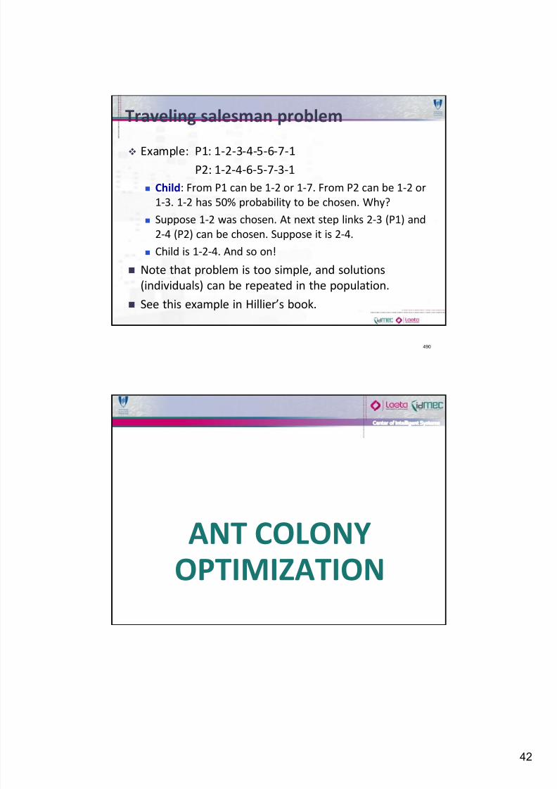
Traveling salesman problem
Example: P1: 1-2-3-4-5-6-7-1
P2: 1-2-4-6-5-7-3-1
Child: From P1 can be 1-2 or 1-7. From P2 can be 1-2 or
1-3. 1-2 has 50% probability to be chosen. Why?
Suppose 1-2 was chosen. At next step links 2-3 (P1) and
2-4 (P2) can be chosen. Suppose it is 2-4.
Child is 1-2-4. And so on!
Note that problem is too simple, and solutions
(individuals) can be repeated in the population.
See this example in Hillier’s book.
490
ANT COLONYOPTIMIZATION
7/24/2019 OD Metaheuristics 2010
http://slidepdf.com/reader/full/od-metaheuristics-2010 43/57
43
Ant Colony Optimization
Marco Dorigo, 1992
Ant Colony Optimiziation is the most used method of
the Artif icial Life algorithms (Wasp, Bees, Swarm).
Applications: Traveling Salesman Problem, Vehicle
Routing, Quadratic Assignment Problem, Internet
Routing and Logistic Scheduling.
There are also some applications of ACO in clustering
and data mining problems.
492
Ant Colony Optimization
Ants can perform complex tasks:
nest building, food storage.
garbage collection, war.
foraging (to wander in search of food).
There is no management in an ant colony
collective intelligence.
They communicate using:
pheromones (chemical substances), sound, touch.
Curiosities:
Ant colonies exist for more than 100 million years.
Myrmecologists estimate that there are around 20,000 species of ants.
493
7/24/2019 OD Metaheuristics 2010
http://slidepdf.com/reader/full/od-metaheuristics-2010 44/57
44
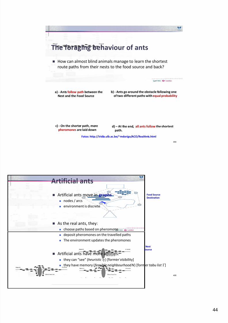
The foraging behaviour of ants
How can almost blind animals manage to learn the shortest
route paths from their nests to the food source and back?
494
a) - Ants follow path between theNest and the Food Source
b) - Ants go around the obstacle following oneof two different paths with equal probability
c) - On the shorter path, morepheromones are laid down
Fotos: http://iridia.ulb.ac.be/~mdorigo/ACO/RealAnts.html
d) – At the end, all ants follow the shortestpath.
Artificial ants
Artificial ants move in graphs
nodes / arcs
environment is discrete
As the real ants, they:
choose paths based on pheromone
deposit pheromones on the travelled paths
The environment updates the pheromones
Artificial ants have more abilities:
they can “see” (heuristic ) [former visibility]
they have memory ( feasible neighbourhood N) [former tabu list ]
495
Nest
Source
Food Source
Destination
7/24/2019 OD Metaheuristics 2010
http://slidepdf.com/reader/full/od-metaheuristics-2010 45/57
45
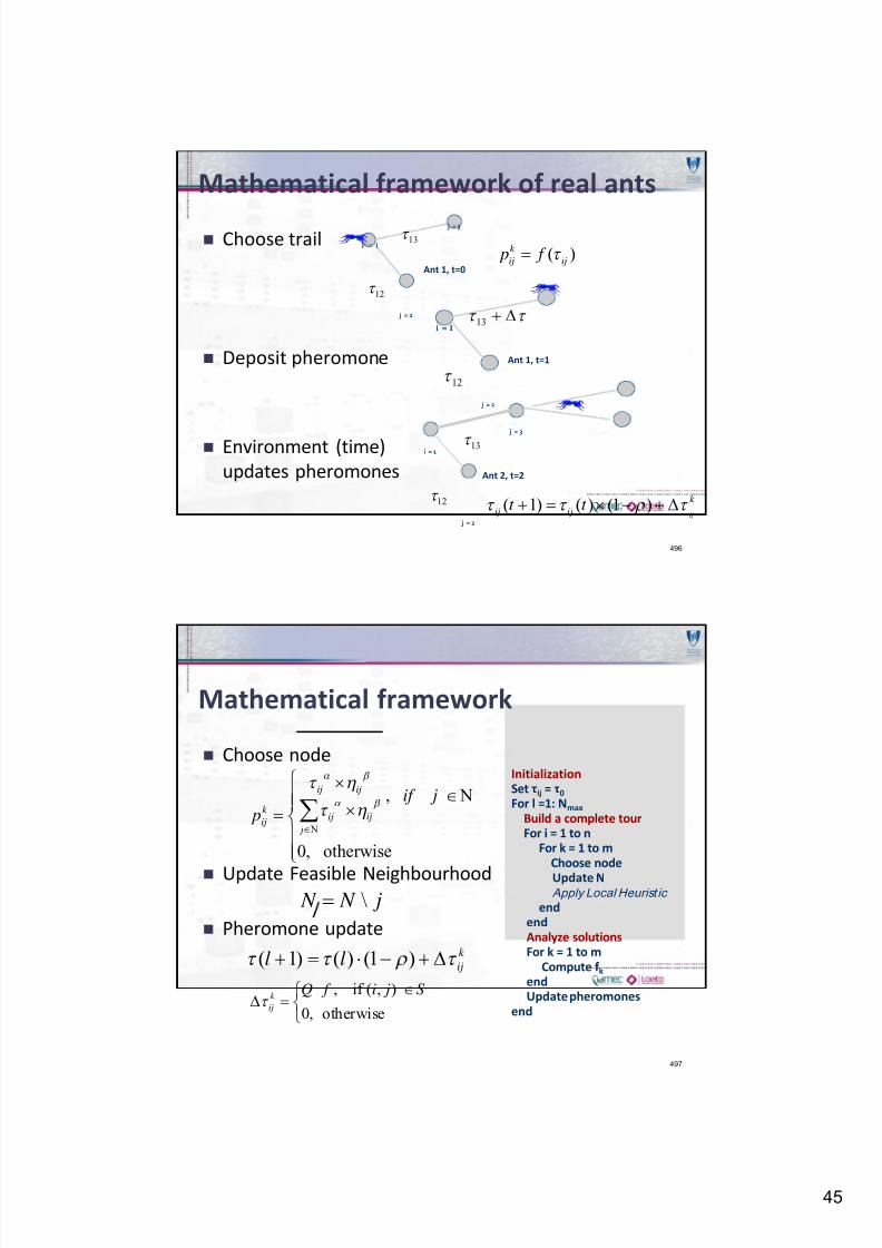
Mathematical framework of real ants
Choose trail
Deposit pheromone
Environment (time)
updates pheromones
496
j = 3
j = 2
Ant 1, t=0
12
i = 113
j = 2
12
i = 113
Ant 1, t=1
Ant 2, t=2
j = 2
12
i = 1
j = 3
13
( 1) ( ) (1 )ij
k
ij ijt t
( )k
ij ij p f
Mathematical framework
Choose node
Update Feasible Neighbourhood
Pheromone update
497
, if ( , )
0, otherwise
k
ij
Q f i j S
\ N N j
k
ijll )1()()1(
,
0, otherwise
ij ij
k ij ij
ij j
if j p
InitializationSet ij = 0
For l =1: Nmax
Build a complete tourFor i = 1 to n
For k = 1 to mChoose node
Update NApply Local Heurist ic
endendAnalyze solutionsFor k = 1 to m
Compute f kendUpdate pheromones
end
7/24/2019 OD Metaheuristics 2010
http://slidepdf.com/reader/full/od-metaheuristics-2010 46/57
46
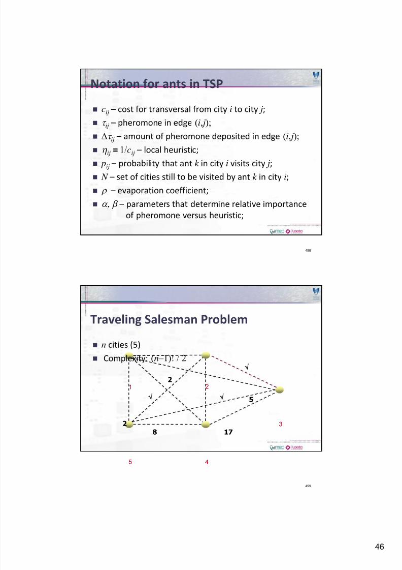
Notation for ants in TSP
cij – cost for transversal from city i to city j;
ij – pheromone in edge (i, j);
ij – amount of pheromone deposited in edge (i, j);
ij = 1/cij – local heuristic;
pij – probability that ant k in city i visits city j;
N – set of cities still to be visited by ant k in city i;
– evaporation coefficient;
– parameters that determine relative importance
of pheromone versus heuristic;
498
Traveling Salesman Problem
n cities (5)
Complexity: (n –1)! / 2
499
1
2
2
5
8 17
2
5 4
3
7/24/2019 OD Metaheuristics 2010
http://slidepdf.com/reader/full/od-metaheuristics-2010 47/57
47
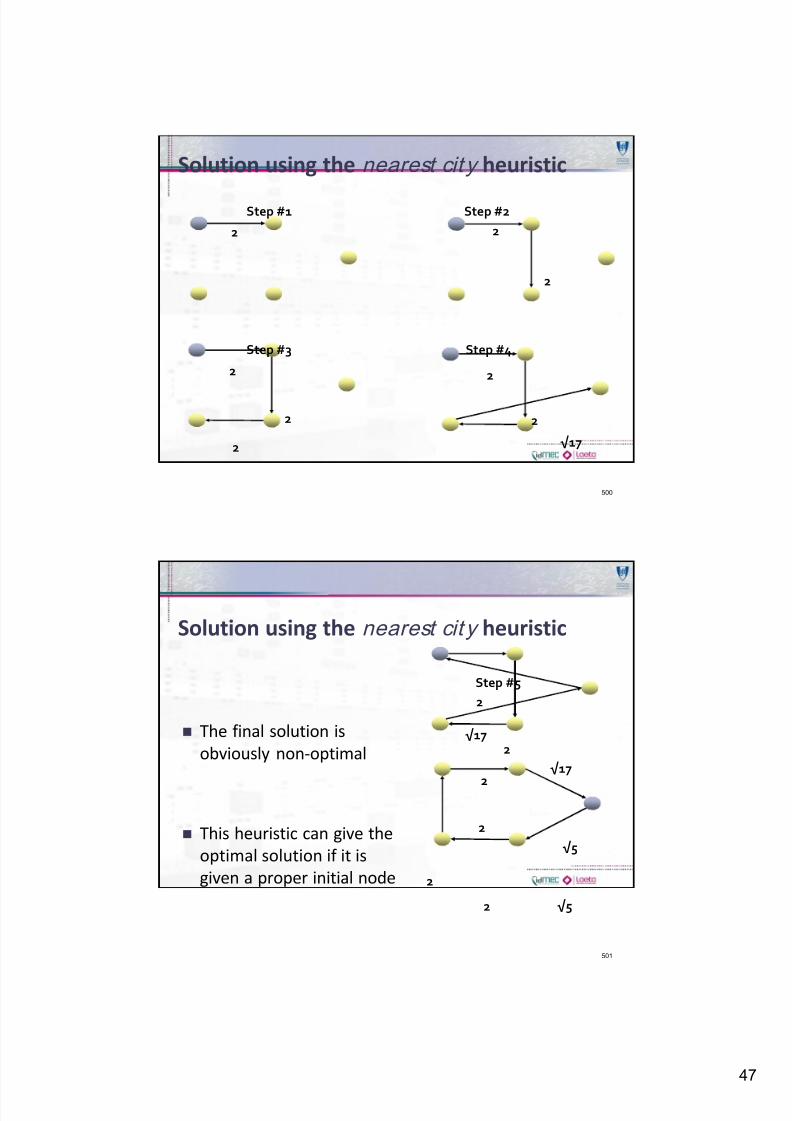
Solution using the nearest cit y heuristic
500
Step #1 Step #2
Step #3 Step #4
2 2
2
2
2
2
17
2
2
Solution using the nearest cit y heuristic
The final solution is
obviously non-optimal
This heuristic can give the
optimal solution if it is
given a proper initial node
501
Step #5
2
2
2
17
17
2
2
2
5
5
7/24/2019 OD Metaheuristics 2010
http://slidepdf.com/reader/full/od-metaheuristics-2010 48/57
48
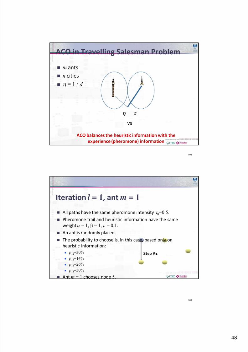
ACO in Travelling Salesman Problem
m ants
n cities
= 1 d
502
vs
ACO balances the heuristic information with the
experience (pheromone) information
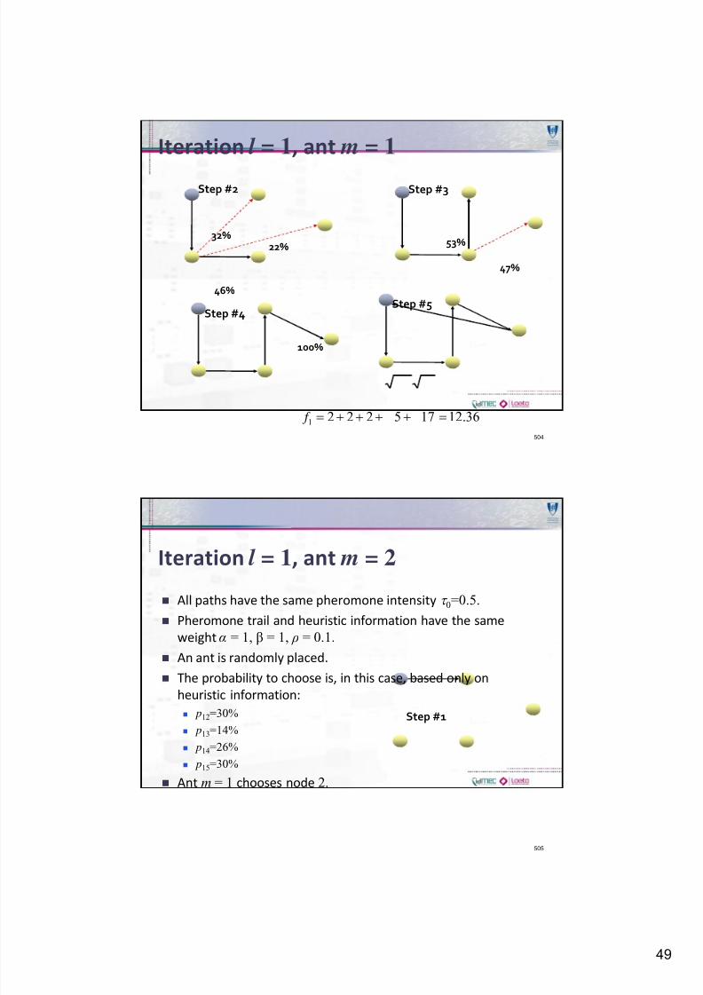
Iteration l = 1, ant m = 1
All paths have the same pheromone intensity 0=0.5.
Pheromone trail and heuristic information have the same
weight = 1, = 1, = 0.1.
An ant is randomly placed.
The probability to choose is, in this case, based only on
heuristic information: p12=30%
p13=14%
p14=26%
p15=30%
Ant m = 1 chooses node 5.
503
Step #1
7/24/2019 OD Metaheuristics 2010
http://slidepdf.com/reader/full/od-metaheuristics-2010 49/57
49
Iteration l = 1, ant m = 1
504
Step #2
46%
32%22%
Step #3
47%
53%
Step #4
100%
Step #5
36.121752221 f
Iteration l = 1, ant m = 2
All paths have the same pheromone intensity 0=0.5.
Pheromone trail and heuristic information have the same
weight = 1, = 1, = 0.1.
An ant is randomly placed.
The probability to choose is, in this case, based only on
heuristic information: p12=30%
p13=14%
p14=26%
p15=30%
Ant m = 1 chooses node 2.
505
Step #1
7/24/2019 OD Metaheuristics 2010
http://slidepdf.com/reader/full/od-metaheuristics-2010 50/57
50
Iteration l = 1, ant m = 2
506
47.10225522 f
Step #2
39%
27%34%
Step #3
65%
35%
Step #4
100%
Step #5
Iteration l = 1, pheromone update
The final solution of ant m=1 is
D=12.36. The reinforcement
produced by this ant m=1 is 0,08.
The final solution of ant m=2 is
D=10,47. The reinforcement
produced by ant m=2 is 0,095!
507
7/24/2019 OD Metaheuristics 2010
http://slidepdf.com/reader/full/od-metaheuristics-2010 51/57
51
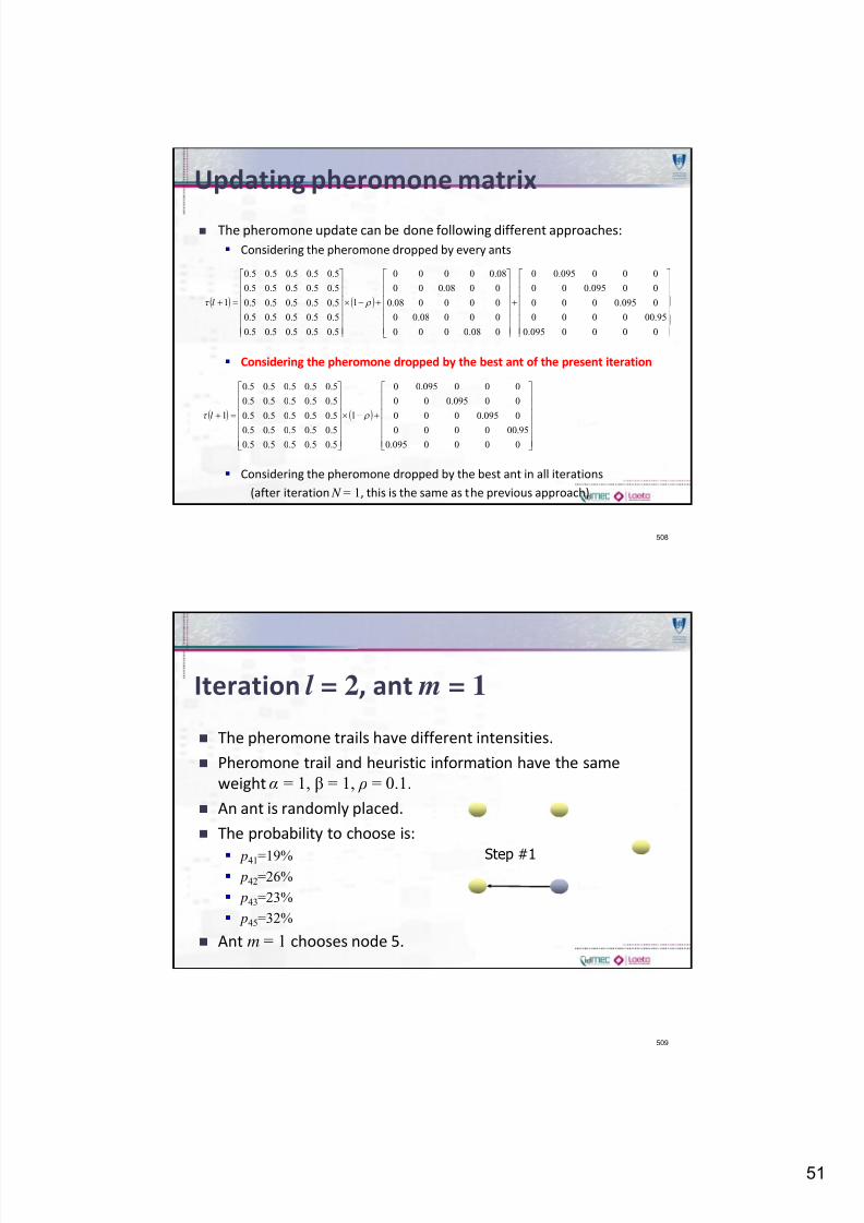
Updating pheromone matrix
The pheromone update can be done following different approaches:
Considering the pheromone dropped by every ants
Considering the pheromone dropped by the best ant of the present iteration
Considering the pheromone dropped by the best ant in all iterations
(after iteration N = 1, this is the same as the previous approach)
508
0000095.0
95.000000
0095.0000
00095.000
000095.00
008.0000
00008.00
000008.0
0008.000
08.00000
1
5.05.05.05.05.0
5.05.05.05.05.0
5.05.05.05.05.0
5.05.05.05.05.0
5.05.05.05.05.0
1 l
0000095.0
95.000000
0095.0000
00095.000
000095.00
1
5.05.05.05.05.0
5.05.05.05.05.0
5.05.05.05.05.0
5.05.05.05.05.0
5.05.05.05.05.0
1 l
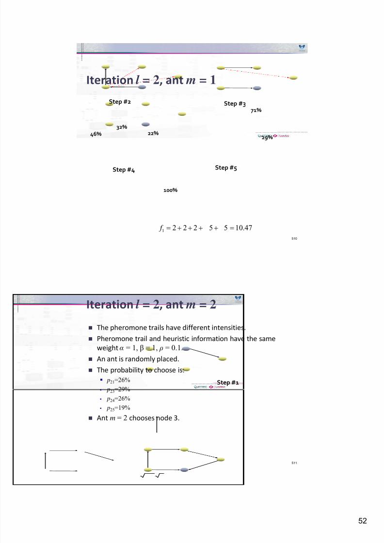
Iteration l = 2, ant m = 1
The pheromone trails have different intensities.
Pheromone trail and heuristic information have the same
weight = 1, = 1, = 0.1.
An ant is randomly placed.
The probability to choose is:
p41=19% p42=26%
p43=23%
p45=32%
Ant m = 1 chooses node 5.
509
Step #1
7/24/2019 OD Metaheuristics 2010
http://slidepdf.com/reader/full/od-metaheuristics-2010 52/57
52
Iteration l = 2, ant m = 1
510
46%
32%22%
Step #3
29%
71%
Step #4
100%
Step #5
47.10552221 f
Step #2
Iteration l = 2, ant m = 2
The pheromone trails have different intensities.
Pheromone trail and heuristic information have the same
weight = 1, = 1, = 0.1.
An ant is randomly placed.
The probability to choose is:
p21=26% p23=29%
p24=26%
p25=19%
Ant m = 2 chooses node 3.
511
Step #1
7/24/2019 OD Metaheuristics 2010
http://slidepdf.com/reader/full/od-metaheuristics-2010 53/57
53
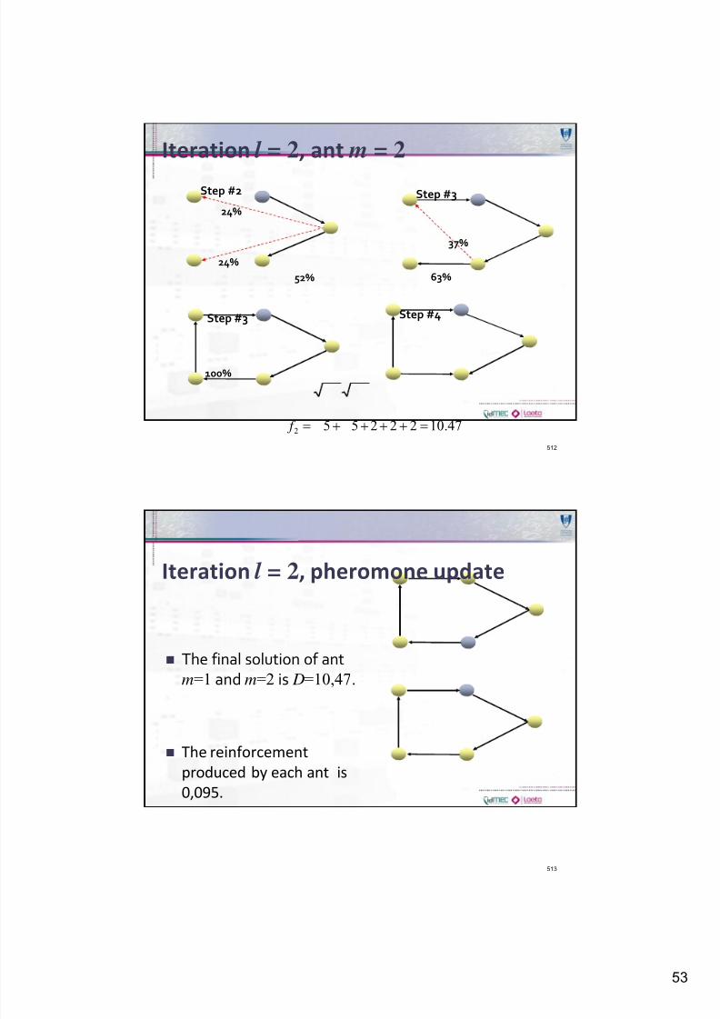
Iteration l = 2, ant m = 2
512
Step #2
52%
24%
24%
Step #3
63%
37%
Step #3 Step #4
47.10222552 f
100%
Iteration l = 2, pheromone update
The final solution of antm=1 and m=2 is D=10,47.
The reinforcement
produced by each ant is
0,095.
513
7/24/2019 OD Metaheuristics 2010
http://slidepdf.com/reader/full/od-metaheuristics-2010 54/57
54
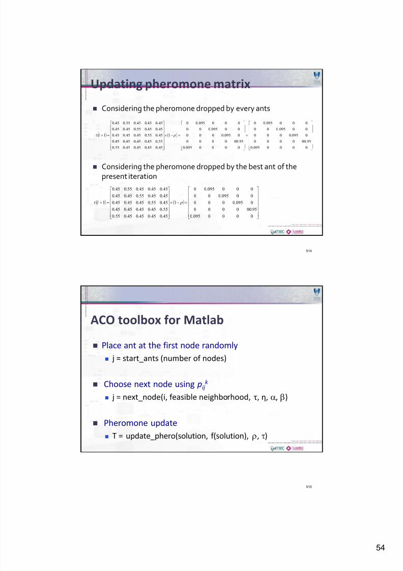
Updating pheromone matrix
Considering the pheromone dropped by every ants
Considering the pheromone dropped by the best ant of thepresent iteration
514
0000095.0
95.000000
0095.0000
00095.000
000095.00
0000095.0
95.000000
0095.0000
00095.000
000095.00
1
45.045.045.045.055.0
55.045.045.045.045.0
45.055.045.045.045.0
45.045.055.045.045.0
45.045.045.055.045.0
1 l
0000095.0
95.000000
0095.0000
00095.000
000095.00
1
45.045.045.045.055.0
55.045.045.045.045.0
45.055.045.045.045.0
45.045.055.045.045.0
45.045.045.055.045.0
1 l
ACO toolbox for Matlab
Place ant at the first node randomly
j = start_ants (number of nodes)
Choose next node using pij k
j = next_node(i, feasible neighborhood, , , , )
Pheromone update
= update_phero(solution, f(solution), , )
515
7/24/2019 OD Metaheuristics 2010
http://slidepdf.com/reader/full/od-metaheuristics-2010 55/57
55
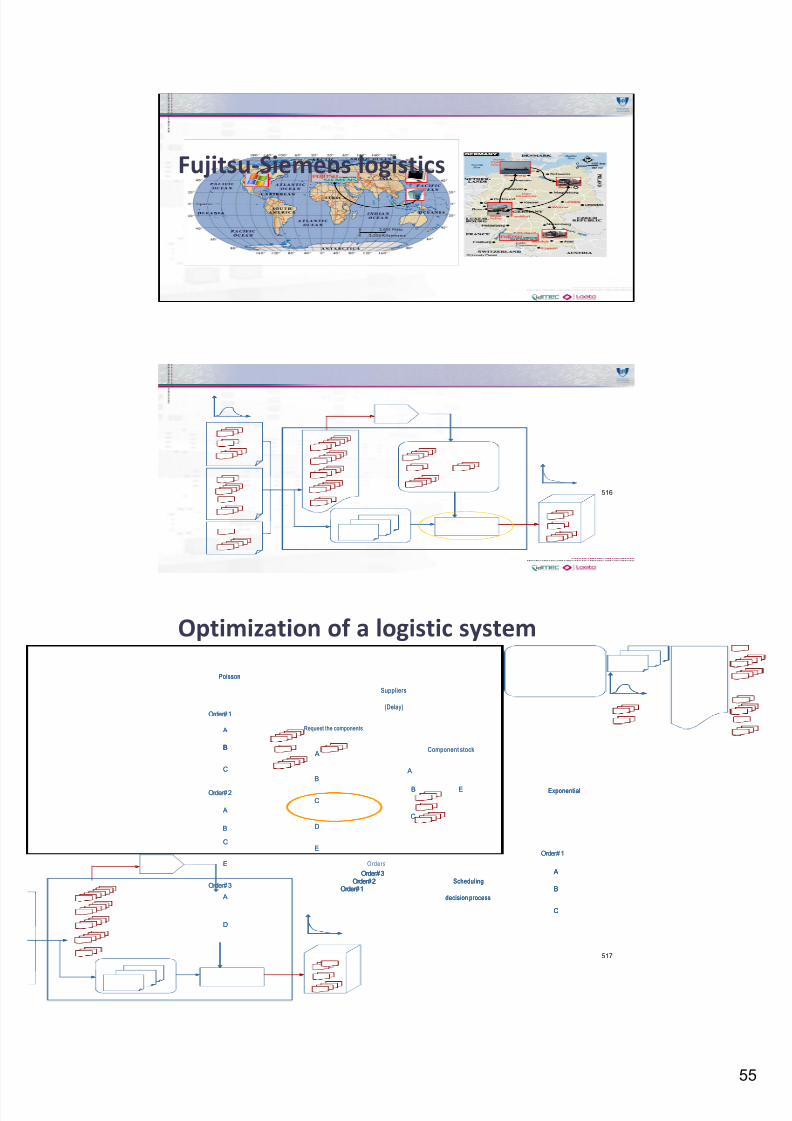
Fujitsu-Siemens logistics
516
Optimization of a logistic system
517
Order #1
Order #2
Order #3Order #1
Order #2
Order #3
Request the components
Suppliers
(Delay)
Component stock
Orders
Scheduling
decision process
Order #1
Poisson
Exponential
A
B
C
B
A
B
C
A
B
C
E
A
D
A
B
C
D
E
B
A
C
E
Order #1
Order #2
Order #3Order #1
Order #2
Order #3
Order #1
Order #2
Order #3
Request the components
Suppliers
(Delay)
Component stock
Scheduling
decision process
Scheduling
decision process
Order #1
PoissonPoisson
ExponentialExponential
A
B
C
B
A
B
C
A
B
C
A
B
C
E
A
D
A
B
C
D
E
B
A
C
E
7/24/2019 OD Metaheuristics 2010
http://slidepdf.com/reader/full/od-metaheuristics-2010 56/57
56
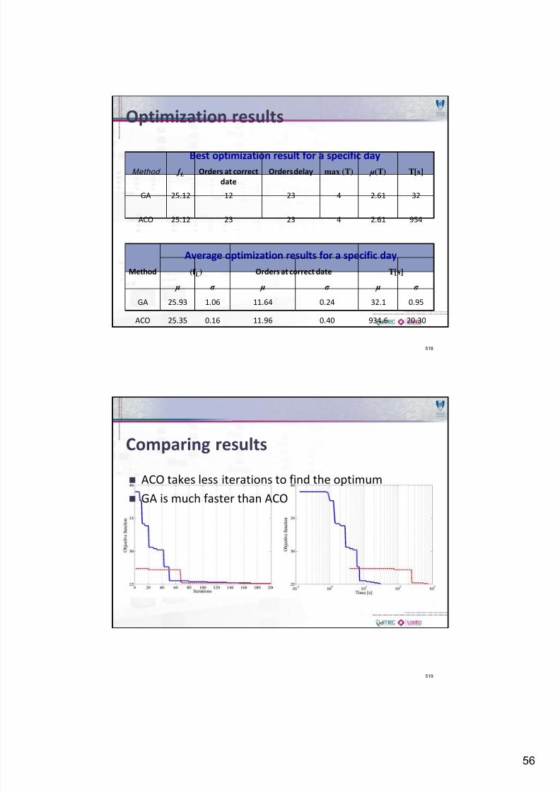
Optimization results
518
Method f L Orders at correct
date
Orders delay max (T) (T) T[s]
GA 25.12 12 23 4 2.61 32
ACO 25.12 23 23 4 2.61 954
Best optimization result for a specific day
Method (f L) Orders at correct date T[s]
GA 25.93 1.06 11.64 0.24 32.1 0.95
ACO 25.35 0.16 11.96 0.40 934.6 20.30
Average optimization results for a specific day
Comparing results
ACO takes less iterations to find the optimum
GA is much faster than ACO
519

7/24/2019 OD Metaheuristics 2010
http://slidepdf.com/reader/full/od-metaheuristics-2010 57/57
Comparing results
GA and ACO present similar performances
ACO has less variation between runs
GA are faster than ACO
Is there any advantage to use ACO?
ACO records information!
How to use this information?
Dynamic environments
Distributed optimization
520