three essays oninequality and economic growth
TRANSCRIPT

- .n 'k L Q T O M A
S f é i / j f a t á
j ^ C ; \ ! . f : c a c i ó n
UNIVERSITAT DE VALENCIA
Facultat d'Economia
Departament d’Análisi Económica
Qi D. 7 H W Z
THREE ESSAYS ONINEQUALITY AND
ECONOMIC GROWTH
Memoria para optar al grado de Doctor en Ciencias Económicas presentada por
Amparo Castelló Climent
Dirigida por
Dr. Rafael Doménech Vilariño
V9BQ
Valencia, Abril de 2002

UMI Number: U607495
All rights reserved
INFORMATION TO ALL USERS The quality of this reproduction is dependent upon the quality of the copy submitted.
In the unlikely event that the author did not send a complete m anuscript and there are missing pages, these will be noted. Also, if material had to be removed,
a note will indicate the deletion.
Disscrrlation Püblish<¡ng
UMI U607495Published by ProQ uest LLC 2014. Copyright in the Dissertation held by the Author.
Microform Edition © ProQ uest LLC.All rights reserved. This work is protected against
unauthorized copying underTitle 17, United States Code.
ProQ uest LLC 789 East Eisenhower Parkway
P.O. Box 1346 Ann Arbor, MI 48106-1346


BiBLIOVcCA ¡
DATA.
SIGNATURA Bíü.T n° u b is: inyiqid u ® ¿ . : m i W e

A mis padres


Contents
Agradecimientos 4
1 Introduction 5
2 Desigualdad y Crecimiento en la OCDE 112.1 Introducción 11
2.2 Modelo Teórico 142.3 Evidencia empírica 322.4 Conclusiones 452.5 Apéndice 47
3 Human Capital Inequality and Economic Growth 513.1 Introduction 513.2 Measuring H um an Capital Inequality 543.3 Variations Within and Across Countries 593.4 Correlation between hum an capital inequality and other
indicators of development 633.5 Hum an Capital Inequality and Economic Growth 6 8
3.6 Conclusions 733.7 Appendix 1 743.8 Appendix 2 80
4 Inequality, Life Expectancy and Development 844.1 Introduction 844.2 The model 8 6
4.3 Inequality and Growth 904.4 Conclusions 1004.5 Appendix 1 1014.6 Appendix 2 102
5 Conclusions 104
References 107
Resumen 112
-3-


Chapter 1IntroductionThe relationship between economic development and income distribution goes back to the influential work of Kuznets (1955). This work analyses the evolution of the inequality in the distribution of income in the course of an economys developm ent process. The "Kuznets hypothesis" maintains the existence of and inverted U shape in the relationship between inequality and development, that is, inequality in the distribution of income increases and later decreases as an economys per capita income rises. Kuznets assumes that in the first stages of development per capita income as well as income inequality increase, since there is a movement of population from the agricultural sector, characterised by a low per capita income, to an industrial sector in which per capita income is higher. Subsequently, when most of the population is in the industrial sector, per capita income increases and income inequality reduces. On the empirical side, it is difficult to confront this hypothesis with data, since there are no income inequality data for a broad period of time that includes the different stages of development in an economy. How- ever, the work of Deininger and Squire (1998) shows that, using the most compre- hensive data set on income inequality to date, the "K uznets hypothesis" has little empirical support.
At the beginning of the last decade emerged some works that, instead of analysing the contemporaneous relationship between per capita income and inequality, they focused on the effect that the initial inequality in the distribution of income and wealth may have on the subsequent economic growth rates. The com- plexity of the relationship between inequality and economic growth has led the- oretical models to analyse this problem from different perspectives. Broadly, the literature has focused on two approaches through which inequality may influence economic growth .1 The first mechanism is usually called the political approach and has been analysed by Bertola (1993), Alesina and Rodrik (1994) or Persson and Tabellini (1994), among others. The main idea of this approach is that, in the political process, those societies with greater inequality in the distribution of wealth will vote for greater redistributive policies than those with a more even distribution. If these redistributive policies are financed by taxes that discourage the investment decisions, the more unequal societies will experience less growth rates. With re-
1 Benabou (19%) or Aghion, Caroli and García-Peñalosa (1999) survey this literture.
-5-

Chapter 1 Introduction
gard to the models included in the second approach, they have in common the assumption of some kind of imperfection in the credit market. The pioneer model of this approach is that of Galor and Zeira (1993).2 In this model, the assumption of non convexities in the accumulation of hum an capital, joint with the assumption of restrictions in the credit market make that the individuáis who inherit an amount lower than a threshold level do not invest in hum an capital and work as unskilled workers. Therefore, in this model the initial distribution of welath determines the average accumulation rates, the higher the number of individuáis with inheritances lower than the threshold level the lower the average hum an capital accumulation rate in the economy.
Whereas there are not consensus about a unique theoretical mechanism that connects the relation between inequality and growth, the empirical work has not helped to clarify totally this relation. Perotti (1996) investigates the relationship between inequality and growth using income distribution data. Firstly, he analy- ses the reduced form relationship between inequality and growth in cross-section regressions. He finds a positive effect from initial equality in the distribution of
oincome on subsequent growth rates. In addition, he analyses some specific chan- nels through which income distribution may influence economic growth. The re- sults give some empirical support for the mechanism of imperfections in the credit market and hum an capital accumulation and a scarce support for the fiscal policy approach .4 Nevertheless, some recent studies have questioned the negative relation between inequality in the distribution of income and economic growth found in previous papers. Using the generalized method of moments technique devel- oped by Arellano and Bond (1991), Forbes (2000) results suggest that in the short and m édium term, an increase in a countrys level of income inequality has a signif- icant positive, instead of negative, relationship with subsequent economic growth rates. In addition, Barro (2000) obtains different effects from inequality in the dis- tribution of income on economic growth in rich and poor countries. The effect is
2 Other models that relate distribution and growth under the presence of imperfections in the credit market include Banerjee and Newman (1993), Aghion and Bolton (1997) or Piketty (1997).3 A negative relationship between income inequality and growth in cross-section regres- sion is also found in Alesina and Rodrik (1994), Persson and Tabellini (1994) or Clarke (1995).4 In addition, Perotti (1996) obtained evidence in favor of a cross-country negative relation between inequality and economic growth through the sociopolitical instability approach and through the mechanism about education and fertility choices.
-6-

negative in countries with low per capita income levels and positive in countries with high income levels. Some papers have found, however, that it is the distribution of assets instead of income what has a harmful effect on growth. In cross- section regressions, Deininger and Squire (1998) found a negative relation between inequality in the distribution of land and economic growth. In the estimation of a growth equation, once they included the land Gini índex in the set of explana- tory variables, the coefficient of the income Gini index stopped being statistically significant.
On the whole, these studies show that the relation between inequality and economic growth is a complex issue that is far from being completely understood.
The objective of this thesis is to go deeply in some points of this issue. To do this, the thesis consists of three essays that analyse, from different perspectives, the effect that inequality in the distribution of income and wealth may exert on economic growth rates.
Due to the scarce empirical support the political approach has obtained in the literature, the objective of the second chapter is to analyse in more detail its predictions. On this matter, the second chapter takes into account some diíferential characteristics in relation to the precedent empirical works.
In particular, since labour income taxes are quite important in many societies, the first part of the chapter extends Alesina and Rodriks (1994) model to allow the government to finance public spending with taxes on labour income. Consequently, this extensión also requires to modelize labour-leisure choice endo- geneously.
The results of the theoretical model show that the more unequal societies, with the aim of redistributing resources, will vote for greater (lower) taxes on capital (labour) income than those with resources more evenly distributed. In addition, capital (labour) income taxes have a non-linear (positive) effect on economic growth rates. Therefore, this model confers a double role to the government, it can enhance or discourage growth as well as it can redistribute resources. On the one hand, the government provides productive Services that increase the produc- tivity of the private production factors. On the other hand, the financing of such spending requires some taxex that can discourage investment as well as redistribute resources. For example, the tax on capital income discourages the investment of capitalist and, in addition, redistributes in favour of workers.
The theoretical predictions of the model are analysed empirically having into account the following. First, the empirical analysis focuses on the structural
-7-

Chapter 1 Introduction
form of the model, that is, it studies the effect of distribution on the demand of redistributive policies and then studies the influence of such policies on the growth rates. Second, we use the last data set on the distribution of income from Deininger and Squire (1996) in which not only the quantity but also the quality of data has been improved. Third, the empirical analysis focuses on OECD countries since in these countries exist the only homogeneous data set about fiscal variables and it makes sense to pose a democratic voting regime.
Having into account these considerations, the results show no empirical support for the fiscal policy approach. In particular, in those countries in which the fiscal system is more developed and where taxes on the accumulable factors are greater, we do not find evidence of a negative effect of income inequality on economic growth through the fiscal variables. We find that the only variable that has affected negatively per capita income growth rates has been the capital income tax. However, we do not find that more unequal societies have greater capital tax rates.
In the third chapter we compute human capital inequality indicators and analyse the effect of such indicators on economic growth.
Most of the theoretical works that analyse the relationship between inequality and growth refer to inequality in the distribution of assets in the economy. For instance, in the theoretical model analysed in the second chapter, in line with the political approach, individuáis differ in their initial endowments of hum an and physical capital. Likewise, the distribution of wealth is also the relevant distribution in the imperfect credit markets approach since, assuming indivisibilities in the investment projects and credit market restrictions, the initial distribution of wealth determines the number of individuáis that will be able to carry out the investment. However, the scarcity of data on the distribution of wealth for a suf- ficient num ber of countries and periods stems from empirical papers that analyse the effect of inequality on growth using income inequality data to proxy wealth inequality measures. Some exceptions are the works of Alesina and Rodrik (1994) or Deininger and Squire (1998) that include the distribution of land to proxy the distribution of income. Nevertheless, land may be an insufficient indicator of wealth since other components as, for example, hum an capital may be important deter- minants of wealth as well as of economic growth rates.
Therefore, the first objective of the third chapter is to compute a data set on the distribution of education for a broad number of countries and periods. To do so, using the last Barro and Lees (2001) data set on attainment levels we com
-8-
pute a Gini coefficient for 108 countries in the period 1960-2000. With the aim of extending the information provided by the Gini coefficient, we also compute the distribution of education by quintiles. Then, we analyse the evolution of these indicators across countries and over time to end analysing their relation with other indicators of development and with economic growth.
The main conclusions of this chapter are as follows. First, when we analyse the evolution of education inequality over time we observe a convergence process in the Gini coefficients of the countries in the sample. This is due to the fact that, on the one hand, most of the countries have reduced the inequality in the distribution of education over the period and, on the other hand, some of the countries that started with a more even distribution of education in 1960, for example New Zealand, Hungary, Finland, The Netherlands or United Kingdom, have increased inequality in the distribution of education during the period 1960-2000. Second, in the estimation of growth equations, the Gini index of the distribution of education displays more robust results than the Gini index of the distribution of income. In particular, the negative effect of the initial inequality in the distribution of income on economic growth rates, obtained in previous works, disappears when in the set of explanatory variables we indude regional dummies to collect specific char- acteristics of the regions. On the contrary, we obtain a negative effect of the initial inequality in the distribution of education on long run economic growth rates that is robust to the inclusión of regional dummies, the inclusión of other variables cor- related to the distribution of education, the use of different samples and the use of different indicators of education inequality. Finally, the results suggest that most of the negative effect that eduction inequality exerts on economic growth is driven through the negative relation between education inequality and the accumulation of factors.
The fourth chapter deais with the relationship between inequality in the distribution of education, life expectancy and economic growth. This chapter devel- ops an alternative channel that explains why the inequality in the distribution of education in a country may be harmful for its subsequent growth rates.
This new channel is analysed in an overlapping generation model in which individuáis may live at most for two periods. They live for sure until the end of the first period but face and endogenous probability to survive the whole second period. It is assumed that an individuáis life expectancy is conditioned by the fam- ily in which she is born into .5 Given the probability an individual has to survive
5 There are medical studies that point out the important role played by the environment
-9-
Chapter 1 Introduction
the second period, she chooses the time devoted to accumulate hum an capital that maximizes her intertemporal utility function. The results show a positive associ- ation between the survival probability and the time devoted to become educated. It is clear that individuáis will devote more time to accumulate hum an capital the longer the period they have to enjoy the retums of education.
The model is calibrated according to life expectancy data from the World Bank and average years of schooling from Barro and Lees (2001) data set.6 The data show a clear concave relationship between schooling years and life expectancy. This concave relationship is also obtained with micro data by Smith (1999). He uses the Health and Retirement Survey (HRS) for 12,000 American individuáis and analyses the relation between individuáis health and their income or wealth. The results show that the relation between self reported health and income or wealth is non-linear, and that the positive and statistically significant effect of income and wealth on self reported health status decreases as socioeconomic status increases.
The numerical results of the model show múltiple steady states in the evolution of hum an capital. In particular, there are two stable steady states, a low one with no education and a high one with about 16 years of school. The model re- flects the reality of many Latin American, South Asian or South-Saharan African countries in which many individuáis born into poor families whose parents have no education, live for a short period of time, do not go to the school and work as raw workers for all their short lives.
The predictions of the model are similar to those of Galor and Zeira (1993) since in both models the initial distribution of education determines the evolution of the economy. The greater the number of poor individuáis, the lower the average hum an capital and income in the economy. However, the underlying assump- tions are different. Whereas Galor and Zeiras model is based on the assumption of convex technologies in the accumulation of hum an capital and imperfect credit markets, our model is based on the differences in life expectancy among rich and poor individuáis.
in which foetus and newbom live in the emergence of an individuáis future disease. Re- cently, Case Lubostky and Paxon (2001) also give evidence of a positive relationship between household income and children health.6 Although the best data to calibrate the survial probability function are micro data, there are not available surveys that report sufficient answers about parents education and off- springs life expectancy.
-10-
Capítulo 2 Desigualdad y Crecimiento en la OCDE
2.1 IntroducciónEn los últimos años un gran número de estudios han analizado las causas de las distintas tasas de crecimiento que se observan en los países. Una parte de esta literatura ha examinado el efecto de la desigualdad en la distribución de la renta sobre el crecimiento económico, señalando varios mecanismos a través de los que la de-•isigualdad puede afectar al crecimiento. El enfoque concreto, sobre el que se va a profundizar en este capítulo es el denominado de política fiscal, del que los modelos teóricos de Bertola (1993), Persson y Tabellini (1994) y Alesina y Rodrik (1994) son pioneros. Estos trabajos coinciden en señalar que en los países democráticos, donde las preferencias de los votantes influyen en las decisiones políticas del gobierno, las sociedades con gran desigualdad en la distribución de la renta presentarán mayor demanda de políticas redistributivas. Si estas políticas redistributivas desincentivan la inversión y el crecimiento es endógeno, el resultado será una reducción de las tasas de crecimiento económico. En consecuencia, la contrastación empírica de estos resultados obliga a analizar dos tipos de mecanismos. El primer mecanismo, llamado mecanismo político, se centraría en demostrar si mayor desigualdad en la distribución de la renta implica mayor demanda de políticas re- distributivas. El segundo, llamado mecanismo económico, debe comprobar si este incremento en las políticas redistributivas tiene un efecto negativo sobre la inversión y sobre el crecimiento económico.
Parte de la evidencia empírica realizada hasta el momento se ha basado en la estimación de una forma reducida, donde se toma una ecuación básica de crecimiento y se añade una variable de distribución de la renta al conjunto de variables explicativas. A partir de este enfoque, Alesina y Rodrik (1994) obtienen evidencia a favor de la influencia negativa que la desigualdad en la distribución de la renta
1 Dentro de esta literatura, se pueden distinguir, a grandes rasgos, tres enfoques: el enfoque de política fiscal, con los trabajos de, por ejemplo, Alesina y Rodrik (1994) y Persson y Tabellini (1994); el trabajo de Alesina y Perotti (1996) se centra en el enfoque de inestabilidad sociopolítica y, por último, Galor y Zeira (1993), entre otros, analizan el efecto de la desigualdad sobre el crecimiento a través de la existencia de restricciones en el mercado de crédito.
-11-

Capítulo 2 Desigualdad y Crecimiento en la OCDE
tiene en las tasas de crecimento económico. Sin embargo, la estimación de esta forma reducida no recoge el mecanismo por el que la distribución de la renta afecta al crecimiento. Para ello es necesario estimar una forma estructural que recoja los dos mecanismos que la teoría predice. Los trabajos que han adoptado esta vía son los de Persson y Tabellini (1994) y Perotti (1996). Ambos trabajos coinciden en sus resultados sobre el mecanismo político, al obtener una relación negativa entre igualdad de la renta y variables fiscales redistributivas, aunque los coeficientes estimados no son estadísticamente significativos. Además, los resultados obtenidos para el mecanismo económico han sido poco satisfactorios y, en algunas ocasiones, contradictorios. Mientras Persson y Tabellini obtienen coeficientes negativos y no significativos para variables de gasto público, Perotti obtiene coeficientes positivos y, en su mayoría, significativos para las variables fiscales que utiliza.
Debido al escaso soporte empírico que ha tenido el enfoque de política fiscal, el objetivo de este capítulo es profundizar en sus predicciones. Para ello, se tienen en cuenta algunas consideraciones diferenciales respecto a los trabajos empíricos precedentes. Estas consideraciones son las siguientes.
Primera, este trabajo se centra en la vertiente impositiva del enfoque de política fiscal, a diferencia de los trabajos precedentes en los que las variables fiscales incluían tanto variables de gasto como de ingreso. La elección de la vertiente impositiva se debe a que son los impuestos y no el gasto redistributivo los que tienen un impacto negativo en el crecimiento económico.2
Segunda, dado que el modelo de financiación de muchas economías incluye tanto imposición del trabajo como del capital, es posible que la falta de evidencia empírica se deba a que, además de analizar la relación entre desigualdad, imposición del capital y crecimiento económico, se tenga que considerar también la importancia de la imposición del trabajo en esta relación. Es por ello que en el modelo teórico de la segunda sección se amplía el modelo de Alesina y Rodrik (1994) para incluir la posibilidad de que el gasto público se financie con un impuesto sobre los rendimientos del trabajo.
Tercera, los trabajos precedentes han utilizado datos de baja calidad sobre las variables de desigualdad en la distribución de la renta. En este trabajo se utiliza la base de datos de Deininger y Squire (1996), donde tanto la cantidad como la calidad de los datos ha sido mejorada. No obstante, hay que señalar que las predicciones de los modelos teóricos se basan en desigualdad en la distribución
2 Algunos trabajos señalan que el gasto público redistributivo tiene un efecto positivo sobre las tasas de crecimiento económico. Véase, por ejemplo, Perotti (1996).
-12-

Sección 2.1 Introducción
de la riqueza. Sin embargo, aunque la correlación entre ambas variables no es tan alta como se esperaría, la disponibilidad de datos sobre distribución de la renta para un amplio número de países y períodos hace que, en los análisis empíricos que incluyen varios países, se utilicen datos sobre distribución de la renta para aproximar la distribución de la riqueza.
Finalmente, la evidencia empírica se centra en los países donde los sistemas fiscales están más desarrollados. La razón para la elección de los países de la OCDE es doble. En primer lugar, es en estos países donde existe una base de datos homogénea sobre variables fiscales. En segundo lugar, en todos estos países existe un régimen democrático y por tanto, tiene sentido plantearse los efectos de la desigualdad sobre la estructura fiscal.
Para analizar la relación entre desigualdad, imposición y crecimiento, en la primera parte del capítulo, se parte de un modelo teórico en línea con el modelo de Alesina y Rodrik (1994) y se amplía en dos vertientes. En primer lugar, se incluye la posibilidad de que el gasto público se financie con un impuesto sobre los rendimientos del trabajo. En segundo lugar, se permite a los individuos elegir las cantidades óptimas de trabajo que están dispuestos a ofrecer.
La elección del modelo de Alesina y Rodrik (1994) como punto de partida se debe a que es un modelo sencillo que permite establecer la relación cualitativa entre las variables relevantes del modelo que posteriormente se analizan en la evidencia empírica. Una de las características de la metodología de Alesina y Rodrik (1994), al igual que la utilizada por Bertola (1993), es que los individuos realizan las votaciones en el momento inicial y éstas permanecen constantes en el tiempo. A este respecto, el trabajo de Krusell, Quadrini y Ríos-Rull (1997) pone de manifiesto que los resultados cuantitativos del modelo de Alesina y Rodrik (1994) cambian cuando los procesos de votación son dinámicos, es decir, cuando las votaciones en el modelo se realizan secuencialmente. Sin embargo, la relación cualitativa entre las variables, que es la verdaderamente relevante para las secciones posteriores de este trabajo, no cambia.
Los principales resultados del trabajo son los siguientes. En la parte teórica, por lo que respecta al mecanismo político (relación entre desigualdad en la distribución de la renta y elección de la imposición óptima), los resultados indican que cuanto mayor es la desigualdad en la distribución de los factores de la sociedad, mayor es el impuesto sobre el capital óptimo y menor el impuesto sobre el trabajo óptimo. En cuanto al mecanismo económico (efecto de la imposición sobre el crecimiento económico), se obtiene que la imposición sobre el capital tiene
-13-

Capítulo 2 Desigualdad y Crecimiento en la OCDE
un efecto no lineal sobre la tasa de crecimiento económico y que la imposición sobre el trabajo tiene un efecto positivo sobre la misma. Por tanto, en este modelo existe una disyuntiva entre políticas redistributivas y políticas que favorecen el crecimiento. Por lo que respecta a los resultados empíricos, en la estimación de la forma estructural del modelo no se obtienen resultados robustos acerca de la relación entre desigualdad y crecimiento a través de la influencia de las variables impositivas en la muestra utilizada de países de la OCDE. En particular, las variables fiscales que dan soporte empírico al mecanismo político no lo dan al mecanismo económico y viceversa.
La organización del capítulo es la siguiente. En la sección segunda se presenta un modelo de crecimiento endógeno, con el que se identifican los principales canales por medio de los cuales la distribución de la renta puede influir sobre el crecimiento de la renta per cápita a largo plazo. La sección tercera ofrece la evidencia empírica, a través de la estimación de una forma estructural, para los países de la OCDE en el período 1960-1995. Por último, en la cuarta sección se presentan las principales conclusiones.
2.2 Modelo TeóricoEl análisis del papel de la desigualdad en la distribución de la renta sobre la estructura impositiva de una economía y sobre el crecimiento económico, que se presenta a continuación, se realiza en un modelo de crecimiento endógeno para una economía cerrada con trabajo y capital como factores primarios de producción, en el que la producción privada requiere la provisión de servicios públicos, bajo el supuesto de que la función de producción presenta rendimientos constantes a escala para los factores acumulables. Si se utiliza una función de producción tipo Cobb-Douglas, la producción agregada viene dada por:
Yt = A K ? L ] -ag \ - a (2 .1 )
donde 0 < a < l . La función de producción es una adaptación de Barro (1990). La variable A representa el nivel de la tecnología, K t y Lt son los stocks de capital y trabajo agregado, respectivamente, donde K t incluye el capital físico y humano. La variable gt es el gasto público por trabajador. Por lo que el gasto público es un bien rival, ya que es el gasto público por trabajador lo que entra en la función
-14-

Sección 2.2 Modelo Teórico
de producción y no el gasto público total.3 Para simplificar, se considera que el producto consiste en un bien homogéneo que puede destinarse indistintamente al consumo o a la inversión y su precio es fijado a la unidad.
En este modelo, al sector público se le atribuye un doble papel, por una parte el gasto público favorece el crecimiento económico mediante la provisión de servicios productivos y, por otra, la financiación de dicho gasto requiere alguna medida impositiva que puede desincentivar la inversión y, a su vez, actuar como política redistributiva. Por tanto, en este modelo, existe un trade-off entre crecimiento y redistribución .4 La interacción entre políticas redistributivas y políticas que favorecen el crecimiento se analiza a través de dos tipos impositivos. Primero, se detalla la influencia de un tipo impositivo sobre los rendimientos del capital (en línea con el trabajo de Alesina y Rodrik, 1994) y, posteriormente, se realiza el análisis cuando el gasto público se financia con un impuesto sobre los rendimientos del trabajo.
2.2.1 Impuesto sobre los rendimientos del capital- Relación entre la imposición del capital y la tasa de crecimiento económico.
Para financiar el gasto en servicios públicos, el gobierno tiene acceso a un impuesto sobre los rendimientos del capital. El gobierno equilibra el presupuesto en cada período de modo que:
9t = rtktTk (2.2)
siendo r k el tipo impositivo sobre el capital.En un contexto de mercados competitivos, la maximización del beneficio
implica que la tasa de rendimiento del capital y el salario vienen determinados por sus respectivas productividades marginales:
r t = (aA r£ _Q)« (2.3)
3 Se incluye el gasto público por trabajador para evitar problemas de escala. Si en la función de producción se incluye el gasto público agregado, un incremento en la escala, representado por L, aumenta los rendimientos del capital después de impuestos y la correspondiente tasa de crecimiento de la renta per cápita de la economía.4 Aghion, Caroli y García-Peñalosa (1999) demuestran que, en un contexto de riesgo morale imperfecciones en el mercado de crédito, la redistribución de la renta puede tener unefecto positivo sobre el crecimiento.
-15-

Capítulo 2 Desigualdad y Crecimiento en la OCDE
wt = (1 - a)A« [o rk \ 1 ^ (2.4)■Lit
Ambas productividades son crecientes en r k pues mayores impuestos permiten mayor gasto público en servicios productivos para un stock de capital dado. Además, el producto marginal del capital, rt/ es invariante en K t, evitando la aparición de rendimientos decrecientes.5
La economía está poblada por n agentes heterogéneos que difieren en sus dotaciones iniciales de capital. En t = 0 cada individuo recibe una dotación de capital kg y elige el número de horas de trabajo que está dispuesto a ofrecer.6 Así,
nel stock agregado de capital en el período cero es K a = A;* y el número total
i=ln
de horas de trabajo ofrecidas viene expresado por L a = ̂ ll0 La dotación relativaí=i
de factores de cada individuo se recoge en la siguiente expresión:
At " « / * ) ' '5)Cuanto m ayor es X] mayor es la dotación relativa de trabajo del individuo
i. En el caso extremo en el que todo el stock de capital estuviera en manos de un único agente, la dotación relativa de factores del individuo i {k\ = 0 ) implica que X\ -» oo.
La renta netta de impuestos del individuo i depende de su dotación de factores y del rendimiento de los mismos:
y\ = wt l\ + rt ( 1 - Tk)k\ (2.6)
Nótese que,, por una parte, el impuesto afecta directamente a los propietarios de capital alterando sus incentivos a acumular y, por otra, al ser Wt creciente en
5 Si se sustituyen lias ecuaciones (2.2) y (2.3) en (21) se obtiene: Yt = .4“ (cxTk)~^~Kt- Esta ecuación clarifica que el modelo que representa a esta economía se reduce a una versión del modelo A K donde los rendimientos marginales del factor acumulable permanecen constantes, en lugar de decrecer, con el proceso de acumulación.6 Nótese que, debido a la existencia de agentes heterogéneos en la economía, el capital por trabajador expresado en minúscula (kt = no tiene porque coincidir con las correspondientes variables individuales. Es por ello que, para evitar la confusión, las variables correspondentes a cada agente individual i se expresan con el superíndice i (k\).
-16-

Sección 2.2 Modelo Teórico
r k, el impuesto favorece la renta procedente del trabajo.Tomando los precios de los factores y el comportamiento del gobierno como
dados, cada consumidor elige el nivel de consumo y la cantidad de horas de trabajo que maximizan su función de utilidad intertemporal sujeto a una restricciónrjdinámica. Así, la decisión de consumo-ahorro y trabajo-ocio del individuo i se obtiene de la resolución del siguiente problema de optimización:
rooM a x Uq = [/31n c\ + a \n (1 — Z¿)] e~ptd t (2.7)ct> li Jo
s.a k\ = y\ — c
donde p es la tasa de preferencia temporal, c\ y l\ denotan, respectivamente, el consumo y el número de horas trabajadas por el individuo i, y ¡3 y cr son las ponderaciones del consumo y del ocio en la función de utilidad, respectivamente. La cantidad de tiempo disponible se normaliza a la unidad. La resolución del ejercicio (2.7), tal y como se obtiene en el apéndice, da lugar a la siguiente senda de consumo óptima:
- = r ( l - r k) - p = <f>(Tk) (2 .8 )&
Nótese que si r k permanece constante, la senda de consumo óptima también será constante. Además, esta senda óptima también coincide con las tasas de crecimiento de k l, C, K , g y w. Por tanto, en este modelo la economía está siempre en situación de crecimiento de estado estacionario en el que todas las variables crecen a una tasa constante determinada por (f)(rk).
Este resultado implica que todos los individuos acumulan a las mismas tasas independientemente de su dotación inicial de factores. Así, la dotación relativa de factores del individuo i (A*) permanece constante en el tiempo.
Por otra parte, utilizando la ecuación (2.8) se puede obtener la relación entre la tasa de crecimiento de la economía y r k . Así, el tipo impositivo que maximiza la tasa de crecimiento viene dado por:
7 Por simplicidad se supone que la elasticidad de sustitución intertemporal es igual a la unidad (6 = 1) y que todo el capital se destruye al final del período (S = 1). Estos supuestos simplificadores no cambian substancialmente los resultados del modelo.
-17-

Capítulo 2 Desigualdad y Crecimiento en la OCDE
0,03
0,02
0,01
0
- 0,01
- 0,020 0,2 0,4 0,6 0,8
Impuesto sobre el capital
Gráfico 2.1: Imposición (tk) y crecimiento
T*k = 1 - a (2.9)
El im puesto sobre los rendimientos del capital es constante y no tiene unQefecto lineal sobre el crecimiento. Para valores de Tfc < r*k domina el efecto que sobre la productiv idad del capital tiene el gasto del gobierno en servicios productivos. Si Tfc > T*k los rendimientos netos del capital disminuyen con incrementos adicionales de r^.. Por tanto, la relación entre la tasa de crecimiento y el tipo impositivo tendrá fo rm a de U invertida alcanzando su máximo cuando T/t = 1 — a. La representación gráfica de dicha relación se puede observar en el Gráfico 2.1. El valor de los parám etros utilizados para la representación de los gráficos 2.1 a 2.6 es A = 0.5; a = 0.6; (3 = 0.5; ít = 0.5; p = 0.02;n = 1 y K = 1.
El resultado obtenido sobre el tipo impositivo óptimo se debe fundamentalmente a la inclusión del gasto público en la función de producción. Cuando
8 El mismo resultado se obtiene en el trabajo de Barro (1990).
-18-

Sección 2.2 Modelo Teórico
el gasto público se considera exógeno en el modelo, los resultados sobre imposición óptima difieren substancialmente. Por ejemplo, en un modelo de crecimiento exógeno con agentes heterogéneos, Judd (1985) obtiene que la imposición óptima sobre el capital en el largo plazo es cero, incluso cuando este impuesto se utiliza para redistribuir recursos de los capitalistas a los trabajadores. Por Otra parte, Chari y Kehoe (1999) analizan la imposición óptima bajo distintas modelizaciones de la economía. En modelos de crecimiento exógeno obtienen que la política óptima en el estado estacionario es no gravar los rendimientos del capital y mantener constante la imposición sobre los rendimientos del trabajo. En particular, en la simulación del modelo para la economía de Estados Unidos obtienen una imposición media igual a cero para el impuesto sobre el capital y una imposición próxima al 20 por ciento, con escasa variabilidad, para el impuesto sobre el trabajo. Cuando el análisis se centra en un modelo de crecimiento endógeno que incluye capital físico y humano, obtienen que la imposición óptima en la senda de crecimiento de equilibrio implica imposición nula para los rendimientos de los factores acumulables, capital físico y humano. No obstante, Jones et al. (1993) analizan la imposición óptima en distintos modelos de crecimiento endógeno y obtienen que el impuesto óptimo sobre el factor capital es distinto de cero cuando en el modelo el gasto público es endógeno. Por tanto, la relación no lineal entre la imposición del capital y la tasa de crecimiento que se observa en el Gráfico 2.1 se debe a que, en este modelo, los impuestos sirven para financiar un gasto público endógeno que aumenta la productividad marginal del factor acumulable.
Además, de las condiciones de primer orden y de la expresión (2.8) se pueden obtener el nivel instantáneo de consumo y la oferta de trabajo óptimos del individuo i:
4 = wl¡ + pk¡ (2 .1 0 )
, i = p a Pkí a m‘ iP + cr) (f3 + a )w t ’
Nótese que el individuo i consume totalmente su renta procedente del trabajo y una fracción constante de su stock de capital. Por otra parte, cuanto mayores el stock de capital del individuo i menor es su asignación óptima de tiempo enel mercado laboral.
Una vez se han obtenido los niveles de consumo y de oferta de trabajo óp
-19-

Capítulo 2 Desigualdad y Crecimiento en la OCDE
timos del individiuo y las sendas de crecimiento de las variables relevantes de la economía, es posilble calcular el impuesto que elegiría un planificador que quisiera maximizar el biemestar de la sociedad. La resolución de este problema se presenta a continuación.- Elección de Tjt por parte de un gobierno que quiere maximizar el bienestar social.
Con la preltensión de obtener el efecto de la proporción relativa de factores de cada indiv iduo en sus preferencias políticas, el problema se va a trasladar a la elección de Tk por un gobernante benevolente cuyo objetivo es maximizar el bienestar del individuo i. Así, el problema de maximización que resolvería el planificador es el qu<e se detalla a continuación:
La resolución de este ejercicio da lugar a la siguiente caracterización im-
que esta expresióm indica que el tipo impositivo óptimo permanece constante en el tiempo. Por tamto, el comportamiento individual de los agentes basado en tipos impositivos constantes es acorde con este resultado.
En el Gráfico 2.2 se observa que el impuesto óptimo elegido por un gobernante que pretende maximizar el bienestar del individuo i es creciente en A*, es
9 Véase el apéndice.10 La elasticidad diel salario es creciente con el tipo impositivo:
M iax Uq [0\n cj + a ln (1 - l¡)] e~pid t (2 .1 2 )
s .a q.c£ = wtllt + pk\
ji _ P vpkj{0 + (t) (J3 + a )w t
K = [irt ( l - T k) - p ] k Í
(2.13)
i nsiendo eWTk la elasticidad del salario frente a variaciones del impuesto. Nótese
£wTh a[(l - a)(P + (r)m(Tk)+crp](1 - a ) 2(/3 4- cr)m(rfc)
donde m(rfc) = A l^a [aTk] X<* .
-20-

Sección 2.2 Modelo Teórico
o
Sío
10,9
0,80,70,60,50,40,30,2
0,1
0
o 1 1,5 2 2,50,5
Dotación relativa de factores
Gráfico 2.2: Dotación de factores (X1) e imposición (rk)
decir, cuanto mayor es la dotación relativa de trabajo por parte del individuo i mayor es su impuesto óptimo deseado. Por tanto, cuanto m ayor es la renta del individuo i, menor es su impuesto sobre el capital óptimo.11
Finalmente, resolviendo la integral de la expresión (2.7) se obtiene:
£/¿ = ^ [ ln 4 + ^ I i l ] + £ l n ( l —¿*) (2.14)
Esta expresión indica que cuando el planificador elige el impuesto que ma-
11 La variación de la renta del individuo i cuando varía su dotación de capital es la siguiente: = — (p+c) + r (l — Tk)- Si la tasa de crecimiento es positiva [r(l — r*¡) > p] —>
> 0, es decir, cuanto mayor es la dotación de capital del individuo i mayor es su renta. Por otra parte, como el individuo i ofrece menos trabajo cuanto mayor es su dotación inicial de capital, X\ será decreciente en k \ . Así, cuanto mayor es la dotación relativa de capital del individuo i menor es X\ y mayor es y\.
- 21-

Capítulo 2 Desigualdad y Crecimiento en la OCDE
ximiza el bienestar del individuo i considera, por una parte, el efecto que el impuesto tiene sobre sus niveles de consumo y oferta de trabajo iniciales y, por otra, el efecto que tiene en la tasa de crecimiento 0 (Tjt).
De los resultados obtenidos anteriormente se pueden sacar las siguientes conclusiones.
Primero, cuanto mayor es la dotación relativa de capital del individuo i (mayor es su renta), menor es su impuesto óptimo sobre los rendimientos del capital.
Segundo, si e l gobierno financia la provisión de servicios productivos con un impuesto sobre los rendimientos del capital y el individuo i no es un capitalista puro, su im puesto óptimo deseado no coincidirá con aquel que maximiza la tasa de crecimiento. Nótese que si el individuo i es un capitalista puro (A1 = 0), el impuesto ideal que elegiría sería r k = 1 — a (véase el Gráfico 2.2), que coincide con aquel que m axim iza la tasa de crecimiento. Esto se debe a que para un capitalista puro el nivel de consumo óptimo se determina eligiendo Tk que maximiza
1 9la tasa de acumulación del capital. Sin embargo, cuando A1 > 0 el impuesto óptimo deseado será mayor que r*k ya que, en este caso, el nivel de consumo depende del salario* y éste es creciente en t*., con lo cual un gobierno que pretenda maximizar el bienestar de un individuo con A1 > 0 no maximizará la tasa de crecimiento económico.
En un contexto en el que la elección de los individuos es única y las preferencias varían de form a monótona con la dotación de factores de los individuos, es posible establecer e l impuesto óptimo que elegiría una sociedad mediante la regla de la mayoría sim ple. En tal caso, la política elegida representaría el impuesto ideal escogido po r el votante mediano en relación con su dotación relativa de factores Am.13 En u n a sociedad donde los factores productivos están distribuidos con la máxima igualdad, todos los individuos tienen la misma dotación relativa de factores tal que X% = Am = 1. En este caso, la dotación relativa de factores del votante medio coincide con la dotación relativa de factores del votante mediano. De este modo, se puede tomar como indicador de desigualdad en la distribución de los factores la siguiente expresión:
r)= X m - l (2.15)
12 Si el individuos, es un capitalista puro (il\ = 0), su nivel de consumo es c\ = pk\.13 Véase Grandmcmt (1978).
-22-

Sección 2.2 Modelo Teórico
Por tanto, cuanto mayor es 77, más alejada está la dotación relativa de factores del votante mediano de la dotación relativa de factores de una sociedad totalmente igualitaria. Además, como Am está relacionada negativamente con y m, una sociedad tendrá mayor desigualdad en la distribución de la renta cuanto menor sea la dotación relativa de capital del votante mediano.
Para finalizar con el análisis del mecanismo político, es necesario tener en cuenta que los procesos de decisión política de las economías son dinámicos, es decir, no se realizan una sola vez y tienen un efecto perpetuo sino que cambian a lo largo del tiempo. Esta consideración pone de relieve las limitaciones del modelo teórico en el proceso de elección, puesto que este trabajo comparte el problema metodológico de Alesina y Rodrik (1994) y Bertola (1993) en cuanto que la elección política se realiza en el momento inicial y permanece constante a lo largo del tiempo. El problema que presentan este tipo de modelos es que la elección de la política actual no tiene en cuenta las repercusiones que dicha elección tendrá en los precios, asignaciones y distribución de la riqueza en el futuro y, por tanto, en las elecciones de política sucesivas.
Por tanto, habría que preguntarse si los resultados obtenidos en el mecanismo político cambian cuando el votante mediano se comporta racionalmente en la elección óptima de su senda impositiva, es decir, cuando tiene en cuenta las repercusiones que su elección de política actual tendrán en el futuro. La respuesta es que habría un cambio cuantitativo en los resultados pero no un cambio cualitativo, tal y como muestran Krusell, Quadrini y Ríos-Rull (1997). En este trabajo, los autores definen un nuevo concepto de equilibrio en el que los agentes se comportan racionalmente tanto en la elección de sus asignaciones como en sus decisiones de política óptimas. En tal caso los resultados del mecanismo político difieren cuantitativamente, pero no cualitativamente, de los obtenidos en un proceso de votación única al comienzo del período. Concretamente, Krusell, Quadrini y Ríos-Rull (1997) obtienen que el tipo impositivo sobre la renta que elegiría un votante mediano con riqueza inferior (superior) a la media en el equilibrio politicoeconómico sería mayor (menor) que en el modelo donde los impuestos son elegidos en el período cero. Según los autores, en el caso en el que el votante mediano tiene una riqueza inferior a la media, el requisito de consistencia temporal del equilibrio político-económico es lo que hace que los impuestos sean más altos que los calculados eligiendo una secuencia constante en el período cero. La razón es que en el equilibrio político-económico el votante mediano internaliza las implicaciones que su elección de política actual tiene sobre la redistribución de la riqueza
-23-

Capítulo 2 Desigualdad y Crecimiento en la OCDE
y, por tanto, sobre la elección de políticas futuras y no lo hace en el caso de una elección en el m om ento inicial.
Para analizar más detalladamente las causas de la discrepancia cuantitativa de los resultados «dependiendo del tipo de votación considerado, se va a calcular el efecto de un carmbio en la política impositiva sobre la distribución de los factores de la sociedad. Para ello, se calcula cómo varía la dotación relativa de factores del votante mediiano cuando varía el tipo impositivo. Sustituyendo l\ y L t en la expresión (2.5) se obtiene:
, m = (i£ )* (? * ) ~ °P „ . „1 (/? + <r)(l - a)m(T¡¡) ( ’
donde k = K /m , k m es la dotación de capital del votante mediano, m ( r k) = A 1̂ a ( a r k)^1~a^ ía y R ( r k ) = {P + tf)(l — a)m (rk) + op. Nótese que si k = km entonces Am = 1, es decir, cuando la dotación relativa de capital del votante mediano coincide con la media, la dotación relativa de trabajo del votante mediano coincide con su dotación relativa de capital.
El efecto d e una variación en el tipo impositivo sobre la dotación relativa de factores del vo tan te mediano es el siguiente:
d \ m ( j p ( l - ¿ )— - = ------- í-i hZl (2.17)d r k OiTk ( p + ( r )m ( T k )
Esta expresión indica que el signo de ta derivada dependerá de la dotación relativa de capital del votante mediano respecto a la media. Los casos posibles son los siguientes:
Primer casto. Si k > km (Am > 1), un incremento en r k implica una reducción en Am y, por tanto, una reducción de la desigualdad en la distribución de los factores en la sociedad puesto que Am está más cercano a la unidad. Además, por el resultado de l mecanismo político se sabe que cuanto menor es Am menor es el impuesto elegido por el votante mediano. Por tanto, si los agentes internalizan el efecto del tipo impositivo sobre la distribución futura de factores en el modelo de elecciones sucesivas, votarán por tipos impositivos más altos en el momento actual para beneficiarse de una menor distorsión impositiva en el futuro.
-24-

Sección 2.2 Modelo Teórico
Segundo caso. Si k < km (Am < 1) un incremento de Tk implica un incremento de Am y como en el mecanismo político la elección del impuesto óptimo es creciente con la dotación relativa de factores del votante mediano, un votante racional prevé que cuanto mayor es el impuesto elegido hoy mayor será Am y, por tanto, mayor será el Tk óptimo que se elegirá mañana. Es por ello que en un modelo de elecciones sucesivas, para reducir las distorsiones impositivas en el futuro, los impuestos que se eligen son más bajos que en un modelo donde únicamente se vota al comienzo del período.
Finalmente, cuando k = km {Xm = 1), Tk no tiene ningún efecto sobre la distribución de los factores de la economía y la elección impositiva en el equilibrio político-económico coincide con la elección que se realiza únicamente al inicio del período.
Por tanto, aunque las predicciones cuantitativas del modelo cambian cuando se consideran votaciones sucesivas, la relación cualitativa entre las variables se mantiene, es decir, lo que cambiaría en el Gráfico 2.2 sería la pendiente de la curva pero no el signo de la misma. Así pues, si el impuesto es elegido por la regla de la mayoría, la relación positiva entre la dotación relativa de capital del votante mediano y su impuesto óptimo sobre las rentas del capital se mantiene.
2.2.2 Impuesto sobre los rendimientos del trabajo-Relación entre la imposición del trabajo y la tasa de crecimiento económico.
Una vez analizado cómo puede afectar la desigualdad en la distribución de la renta sobre la fiscalidad del capital y sobre el crecimiento económico, en este apartado se supone que el gobierno financia la provisión de servicios públicos a través de un impuesto sobre los rendimientos del trabajo. De nuevo el gobierno equilibra el presupuesto en cada período, de manera que:
9t = w tTi (2.18)
donde Ti es el tipo impositivo sobre el trabajo.Siguiendo los mismos pasos que en el subapartado 2.2.1, el salario y el tipo
de interés son:
r t = a A ~ [(1 - a )T |]1í a (2.19)
-25-

Capítulo 2 IDesigualdad y Crecimiento en la OCDE
m t = (A (l - a ) r j a ) i ~ (2.20)-Lí
Tanto Wt como vmelven a ser crecientes con el tipo impositivo, ya que mayor gasto público en serwicios productivos favorece la productividad de ambos factores de producción.
La renta neta de impruestos que recibe el individuo i, dada su dotación de capital y la cantidad de tralbajo que está dispuesto a ofrecer, es la siguiente:
y\ = wt { l - T i ) l \ + rtk\ (2.21)
El consum idor resuellve el problema de optimización como el descrito en (2.7), cambiando (2.6) por ('2.21). De la resolución de este ejerdcio se obtiene que en la senda de equilibrio lais tasas de crecimiento son constantes. En particular la senda de crecimiento óptimia de las variables relevantes viene determinada por:
7fc* = 7c< = 1 k = l a = Ig = lY = lw = r - P = £0n) Vz (2.22)
A diferencia del impuiesto sobre el capital, que tenía un efecto no lineal sobre la tasa de crecimiento, tel impuesto sobre el trabajo tendrá un efecto positivo sobre el crecimiento econónnico. Este hecho se debe a que el impuesto sobre el trabajo sirve exclusivamente p>ara financiar un gasto público dedicado a la provisiónde bienes y servicios que faavorecen la productividad de los factores privados deproducción. Por lto tanto, curanto mayor es el impuesto sobre el trabajo, mayor será la provisión de g# y mayor :será el rendimiento neto del capital y, con ello, la tasa de crecimiento económico.144
Con este tipo de finamciación del gasto público la tasa de crecimiento en el estado estacionario es superior a la que se obtiene en una economía donde el gasto público se financia exclusiv/amente con impuestos sobre el capital. En el Gráfico 2.1, se observa quie la tasa dle crecimiento máxima cuando gt se financia con es aproxim adam ente del 2 por: ciento, siendo el impuesto óptimo igual a (1 — a). En
14 Aunque las conclusiones des su trabajo son distintas, Saint-Paul y Verdier (1993) obtienen resultados similares. En su moidelo, los impuestos no distorsionadores sirven para financiar la educación pública. Ademáss, como la acumulación de capital humano es la fuente del crecimiento, aparte de redistritbuir recursos, los impuestos favorecen la tasa de crecimiento de la economía.
-26-
Sección 2.2 Modelo Teórico
0,1
0,08
0,06
0,04
0,02
0
- 0,02
-0,040,2 0,4 0,6 0,80 1
Impuesto sobre el trabajo
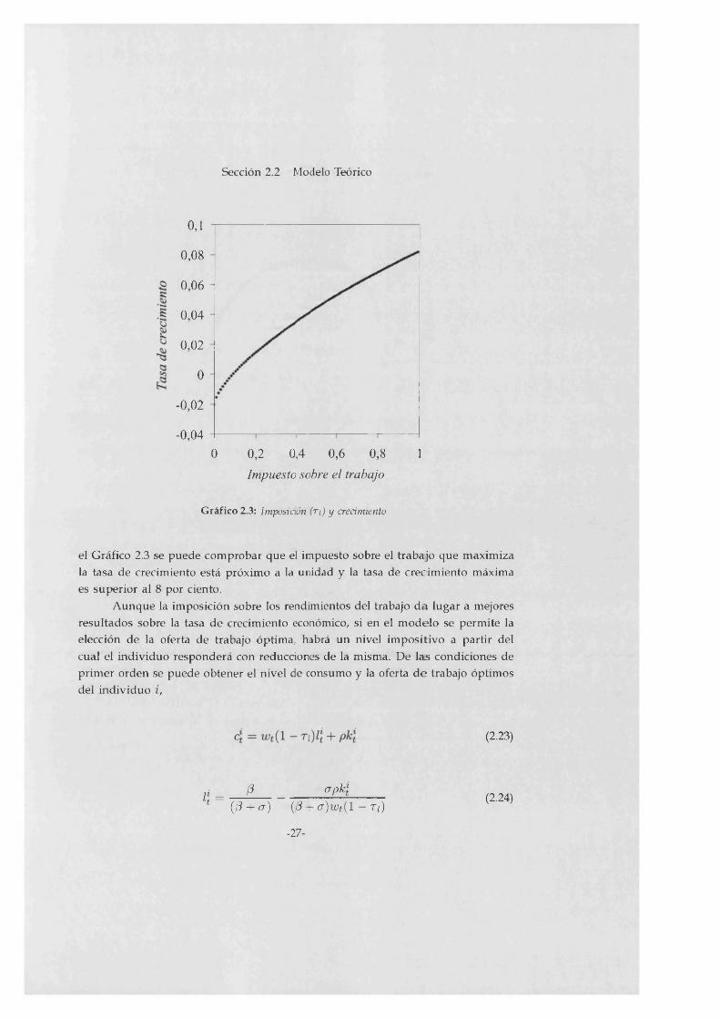
Gráfico 2.3: Imposición ( t ¡ ) y crecimiento
el Gráfico 2.3 se puede comprobar que el impuesto sobre el trabajo que maximiza la tasa de crecimiento está próximo a la unidad y la tasa de crecimiento máxima es superior al 8 por ciento.
A unque la imposición sobre los rendimientos del trabajo d a lugar a mejores resultados sobre la tasa de crecimiento económico, si en el m odelo se permite la elección de la oferta de trabajo óptima, habrá un nivel im positivo a partir del cual el individuo responderá con reducciones de la misma. De las condiciones de prim er orden se puede obtener el nivel de consumo y la oferta d e trabajo óptimos del individuo i,
(2.23)
/ * — Lt ~(3 apk\
(/? + <r) ((3 + o)wt {l - t i )(2.24)
-27-

Capítulo 2 Desigualdad y Crecimiento en la OCDE
0,4
,0
0 0,2 0,4 0,6 0,8
Impuesto sobre el trabajo
Gráfico 2.4: Imposición ( t i ) y oferta de trabajo
al mismo tiempo, se puede calcular la oferta agregada de trabajo de la economía como:
u = E =n/3 o p K t
¿=i (/? + cr) (/? + <7) ^ ( 1 - T i)(2.25)
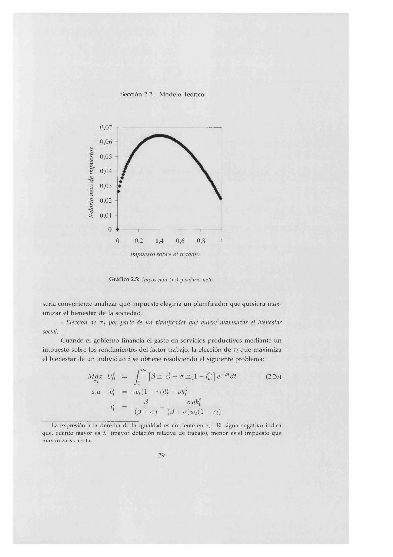
En el Gráfico 2.4 se observa que, a partir de un determinado nivel impositivo, los individuos responden con reducciones de la oferta de trabajo a incrementos en T¡ . Al mismo tiempo, como también tiene un efecto no lineal sobre el salario neto (Gráfico 2.5), cuanto mayor es la proporción de las rentas procedentes del trabajo en la renta total del individuo i, menor será su impuesto deseado.15
No obstante, como al individuo lo que le interesa es maximizar su utilidad,
15 El impuesto sobre el trabajo que elegiría un individuo en relación con su dotación de factores tal que su renta y1 sea máxima, viene recogido en la siguiente expresión:
V = — crp + a(/3 + a) [.4(1 - a)] « t ~
(fi + v) [A ( l-a )] ' ( 1 - a - r i )
-28-
Sección 2.2 Modelo Teórico
0,07
0,06>1Ot¡
I0,05
.« 0,04
S 0,03s:■5 0,02'CO£ 0,01
0 0,2 0,4 0,6 0,8 1
Impuesto sobre el trabajo
Gráfico Z5: Imposición (t¡) y salario neto
sería conveniente analizar qué impuesto elegiría un planificador que quisiera max- imizar el bienestar de la sociedad.
- Elección de Ti por parte de un planificador que quiere maximizar el bienestarsocial.
Cuando el gobierno financia el gasto en servicios productivos m ediante un impuesto sobre los rendimientos del factor trabajo, la elección de T/ que maximiza el bienestar de un individuo i se obtiene resolviendo el siguiente problema:
rooMax Uq = [/3\n cj + crln (l — ZJ)1 e~pidt (2-26)
Tl Jos.a c\ = wt (l — Ti)l\ + pk\
(3 apk¡nLt — (P + <r) (J3 + a)wt ( l - n )
La expresión a la derecha de la igualdad es creciente en r¡. El signo negativo indica que, cuanto mayor es A* (mayor dotación relativa de trabajo), menor es el impuesto que maximiza su renta.
-29-
Capítulo 2 Desigualdad y Crecimiento en la OCDE
kt = (r ~ P)kt
la resolución de este ejercicio da lugar a la siguiente caracterización implícita:
£A r,(1 - T') = - ¿ <227>
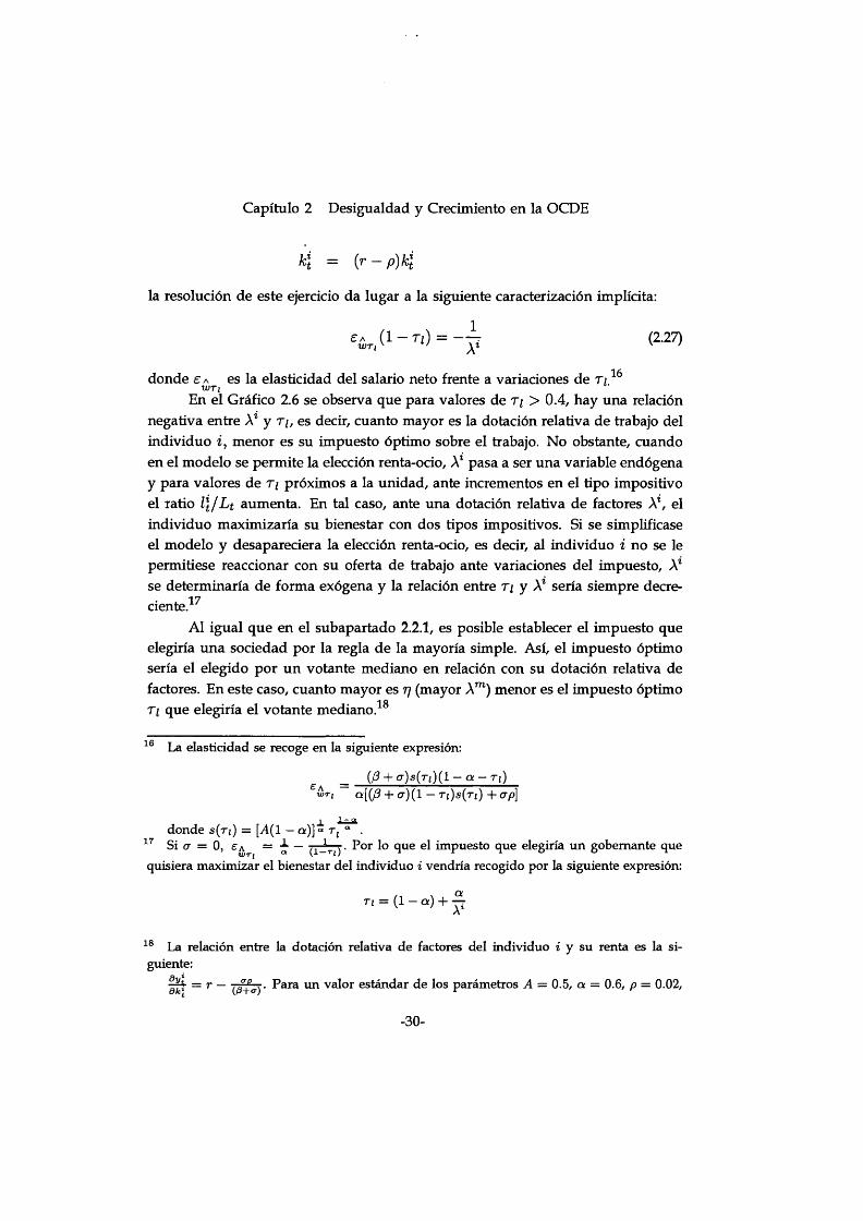
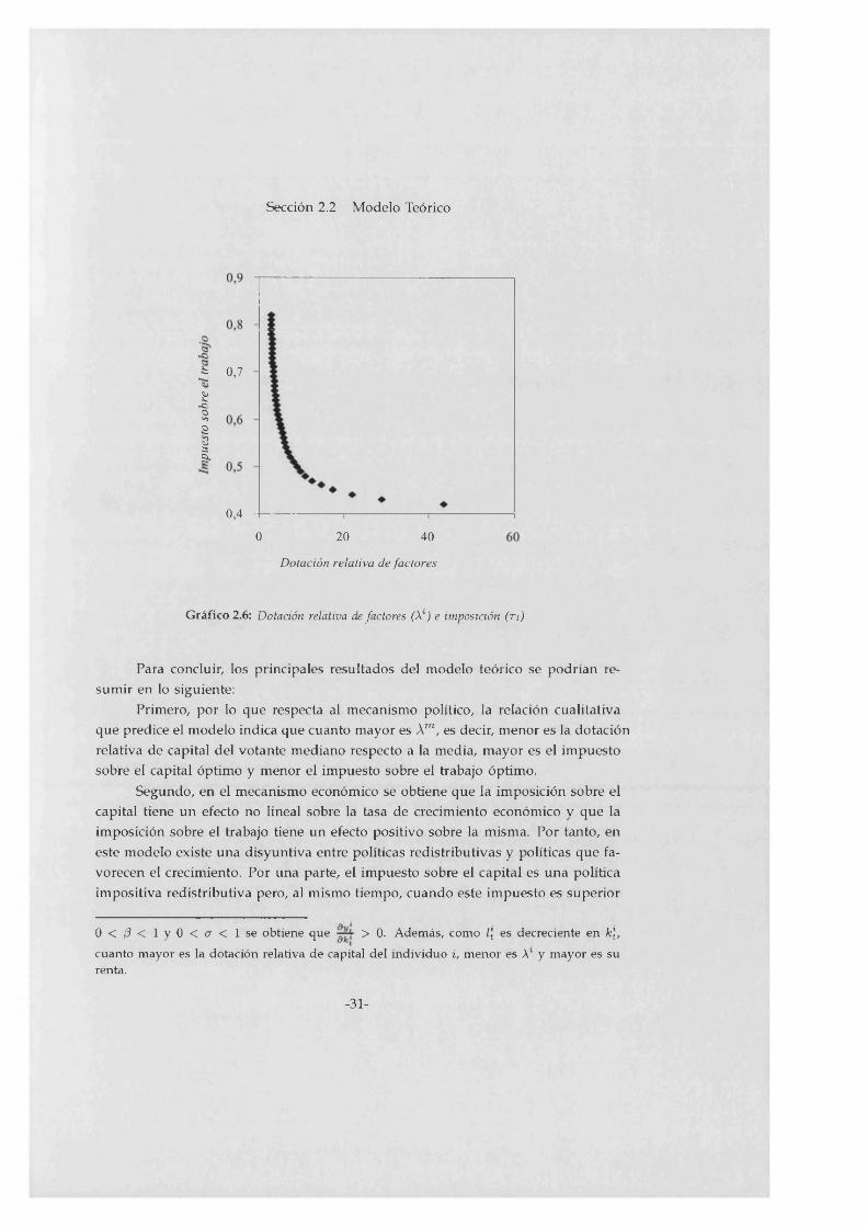
1 f\donde e a es la elasticidad del salario neto frente a variaciones de TiWT¡En el Gráfico 2.6 se observa que para valores de T/ > 0.4, hay una relación
negativa entre X1 y Ti, es decir, cuanto mayor es la dotación relativa de trabajo del individuo menor es su impuesto óptimo sobre el trabajo. No obstante, cuando en el modelo se permite la elección renta-ocio, X1 pasa a ser una variable endógena y para valores de Ti próximos a la unidad, ante incrementos en el tipo impositivo el ratio l \ /L t aumenta. En tal caso, ante una dotación relativa de factores X1, el individuo maximizaría su bienestar con dos tipos impositivos. Si se simplificase el modelo y desapareciera la elección renta-ocio, es decir, al individuo i no se le permitiese reaccionar con su oferta de trabajo ante variaciones del impuesto, A* se determinaría de forma exógena y la relación entre Ti y X% sería siempre decre-
17cíente.Al igual que en el subapartado 2.2.1, es posible establecer el impuesto que
elegiría una sociedad por la regla de la mayoría simple. Así, el impuesto óptimo sería el elegido por un votante mediano en relación con su dotación relativa de factores. En este caso, cuanto mayor es rj (mayor Xm) menor es el impuesto óptimo
1 QTi que elegiría el votante mediano.
16 La elasticidad se recoge en la siguiente expresión:
_ (/3 + a)s(Ti)(l - a - n )£ & r l ck[(/5 + c t)(1 - T i ) s ( t i ) + a p \
x 1-adonde s(rj) = [A(l — a )]« r z “ .
17 Si a = 0, £A = ” — (í-t ,) • P°r 1° que el impuesto que elegiría un gobernante quequisiera maximizar el bienestar del individuo i vendría recogido por la siguiente expresión:
/. \ ocTi = (1 - a) + j r
18 La relación entre la dotación relativa de factores del individuo i y su renta es la siguiente:
ffcj- = r ~ Jp+7)' Para un valor estándar de los parámetros A — 0.5, a = 0.6, p = 0.02,
-30-
Sección 2.2 Modelo Teórico
fe 0,7
Síc§3Sa¡L
0,4
0 20 40
Dotación relativa de factores
Gráfico 2.6: Dotación relativa de factores (X1) e imposición ( t i )
Para concluir, los principales resultados del m odelo teórico se podrían resumir en lo siguiente:
Primero, por lo que respecta al mecanismo político, la relación cualitativa que predice el m odelo indica que cuanto mayor es Am, es decir, menor es la dotación relativa de capital del votante mediano respecto a la media, mayor es el impuesto sobre el capital óptimo y menor el impuesto sobre el trabajo óptimo.
Segundo, en el mecanismo económico se obtiene que la imposición sobre el capital tiene un efecto no lineal sobre la tasa de crecimiento económico y que la imposición sobre el trabajo tiene un efecto positivo sobre la misma. Por tanto, en este m odelo existe una disyuntiva entre políticas redistributivas y políticas que favorecen el crecimiento. Por una parte, el impuesto sobre el capital es una política impositiva redistributiva pero, al mismo tiempo, cuando este impuesto es superior
0 < /? < 1 y 0 < (7 < l s e obtiene que > 0. Además, como l\ es decreciente en k\,cuanto mayor es la dotación relativa de capital del individuo i, menor es A1 y mayor es su renta.
-31-

Capítulo 2 Desigualdad y Crecimiento en la OCDE
a un determinado nivel, un incremento del mismo reduce la tasa de crecimiento económico. Lo contrario ocurre cuando el gasto en servicios productivos se financia con un impuesto sobre el factor no acumulable, es decir, el impuesto sobre el trabajo tiene un efecto positivo sobre el crecimiento pero redistribuye en favor de los propietarios de capital.
2.3 Evidencia empíricaEn esta sección se profundiza en la evidencia empírica sobre la relación entre desigualdad y crecimiento económico, a través de su influencia sobre los tipos impositivos. La organización de esta sección es la siguiente. En primer lugar, se realiza una breve descripción de los datos utilizados. En segundo lugar, se presenta la evidencia empírica de la estimación de la forma reducida. En tercer lugar, se estima la forma estructural, es decir, se analiza el mecanismo político para averiguar de qué manera la desigualdad condiciona la estructura fiscal y se estudia el mecanismo económico que relaciona fiscalidad y crecimiento económico.
2.3.1 Datos utilizadosLa calidad de los datos sobre distribución de la renta ha sido un tema cuestionado por todos los trabajos empíricos realizados sobre distribución de la renta y creci-
19miento. Hasta ahora, los datos generalmente utilizados se basaban en los trabajos de Fields (1989), Jain (1975) y Paukert (1973). Sin embargo, recientemente ha aparecido una nueva base de datos mucho más completa realizada por Deininger y Squire (1996) en el Banco Mundial, en la que tanto la cantidad como la calidad de los datos ha sido mejorada. Al utilizar esta nueva base de datos, los autores encuentran ejemplos que ilustran que las conclusiones a las que llegan algunos estudios anteriores pueden estar sesgadas por la utilización de datos de baja calidad.20
Los datos se corresponden con ingresos de las familias en términos brutos,
19 Véase, por ejemplo, Perotti (1996).20 La base de datos usada por Persson y Tabellini (1994), basada en Paukert (1973), incluye un número de países (Birmania, Chad, Chipre, Benin, Irak, Líbano) para los cuales Deininger y Squire fueron incapaces de encontrar datos de calidad aceptable, un tercio de sus coeficientes de Gini difieren en cinco o más puntos de las observaciones aceptables y únicamente 18 de sus 55 observaciones satisfacen los criterios de calidad. Así, la relación negativa entre desigualdad de la renta y tasas de crecimiento desaparece cuando Deininger y Squire vuelven a hacer las regresiones de Persson y Tabellini usando únicamente 18 (de los 55) datos de alta calidad que contiene la muestra.
-32-

Sección 2.3 Evidencia empírica
es decir, ingresos de las familias antes de deducir los impuestos. Para obteneruna base de datos homogénea entre países, se han construido índices correctorespara aquellos países donde las observaciones eran individuales en términos ne-
21tos. Con estas transformaciones ha quedado una muestra de 17 países para el período 1950-1992. Aunque esta nueva base de datos recoge observaciones de países en desarrollo y desarrollados, el análisis se centrará exclusivamente en los países de la OCDE, puesto que es en estos países donde existe la única base de datos homogénea sobre variables fiscales y porque en todos ellos existe un régimen democrático, en el que tiene sentido plantear la elección de la estructura fiscal. Estados Unidos es el único país que tiene datos para el período completo, en el resto de países las observaciones disponibles empiezan a partir de los años 60. Las observaciones iniciales se toman lo más cerca posible de 1960, año para el cual se mide la tasa media de crecimiento de la renta per cápita, de modo que se asegura la exogeneidad de las variables que recogen la distribución de la renta.
La medida que se va a utilizar para recoger la desigualdad en la distribución de la renta es el coeficiente de Gini, coeficiente basado en la curva de Lorenz que relaciona la proporción de población con la proporción de renta percibida por los distintos estratos de la población. El coeficiente de Gini se medirá en tantos por ciento, por lo que tomará valores entre cero y cien, indicando mayor igualdad de la renta cuanto más próximo a cero se encuentre su valor.
Es necesario destacar que, atendiendo al modelo teórico, en la presente sección sería necesario utilizar un indicador de desigualdad en la distribución de la riqueza en lugar de un indicador de desigualdad en la distribución de la renta. Por ejemplo, Díaz-Giménez, Quadrini y Ríos-Rull (1997) para la economía de Estados Unidos obtienen, por una parte, una alta correlación entre los ingresos laboralesy la renta (0.928) y, por el contrario, una correlación m uy baja entre la riqueza y
00los ingresos laborales (0.230) y entre la riqueza y la renta (0.321). Sin embargo,
21 Para pasar de netos a brutos se ha calculado la media de ambas observaciones para los años disponibles de cada país (Media Gini Bruto/Media Gini Neto)=X y se ha utilizado dicho factor para aquellos países que disponían principalmente de valores netos. El mismo procedimiento se ha seguido para transformar los datos en ingresos procedentes de las familias.
22 La correlación también es muy baja al comparar la concentración en la distribución de la renta y la concentración en la distribución de algunos componentes de la riqueza. Por ejemplo, para una sección cruzada de países, la correlación entre el índice de Gini de la distribución de la renta y el índice de Gini de la distribución de la tierra es 0.39 (Véase Deininger y Squire, 1998) y la correlación entre el índice de Gini de la distribución de la
-33-

Capítulo 2 Desigualdad y Crecimiento en la OCDE
en esta sección se utiliza la distribución de la renta porque no hay disponible una base de datos sobre distribución de la riqueza para un amplio número de países y períodos.
Para las variables impositivas se utiliza la base de datos de Boscá, Fernández y Taguas (1997). Los datos impositivos utilizados se refieren a los tipos impositi-(Vivos efectivos sobre el trabajo y el capital. En cuanto a los datos referidos a la renta real y sus componentes, se han obtenido de la base de datos recogida en el trabajo de Dabán, Doménech y Molinas (1997). La variable de educación utilizada proviene de la nueva base de datos de De la Fuente y Doménech (2001).
2.3.2 Forma reducida: desigualdad-crecimientoDejando a un lado de momento la posibilidad de condicionar con respecto a otras variables, como sugieren Mankiw, Romer y Weil (1992), en principio sí parece que exista cierta relación negativa entre desigualdad de la renta al comienzo del período y la tasa media de crecimiento de la renta per cápita durante los años 1960-1990. Si se divide la totalidad de países para los que se dispone de datos de desigualdad y crecimiento en seis grupos (Este de Asia, Oriente Medio-Norte de Africa, OCDE, Sur de Asia, Africa Sub-Sahariana y América Latina) tal y como muestra el Gráfico 2.7, se observa que América Latina y Africa Sub-Sahariana presentaban un coeficiente de Gini cercano a 50 en los años 60 y sus tasas de crecimiento para el período 60-90 han sido menores al 2 por cien. En cambio, para los países del Este de Asia y OCDE el coeficiente de Gini inicial oscilaba entre 35 y 38 y su crecimiento, en términos medios, ha sido superior al 2,5 por cien. Así, si la muestra incluye la totalidad de países parece que sí existe una relación negativa entre ambas variables, América Latina y Africa Sub-Sahariana son el grupo de países que partían de mayores niveles iniciales de desigualdad de la renta y han crecido menos que aquel grupo de países con distribuciones de la renta más igualitarias (Este de Asia y OCDE).
Sin embargo, esta relación negativa entre desigualdad y crecimiento no es tan evidente cuando el análisis se centra exclusivamente en los países de la OCDE.24 En el Gráfico 2.8 se observa una relación positiva entre el indicador de
renta y el índice de Gini de la distribución del capital humano es 0.27 (Véase el capítulo tercero).
23 Véase Boscá et al. (1997) para una descripción detallada de las definiciones de los distintos tipos impositivos.
24 La muestra la componen los siguientes países de la OCDE: Alemania (AL), Australia (AUS), Bélgica (BEL), Canadá (CAN), Dinamarca (DIN), España (ESP), Estados Unidos (USA),
-34-

Sección 2.3 Evidencia empírica
Este de Asií4,5
• Oriente Medio N. de África♦ OCD1
África S. Sahariana
0 ,5 -
30 35 40 45 50 55
Desigualdad inicial (Gini)
Gráfico 2.7: Tasa de crecimiento de la renta per cápita (60-90) y desigualdad inicial
desigualdad de la renta al comienzo del período y la tasa de crecimiento de la renta per cápita durante los años 1960-1995 para una muestra de 17 países de la OCDE.25 Países como Italia, Irlanda, Francia, Finlandia y Noruega que partían de elevados coeficientes de Gini han crecido, en términos medios, más que aquellos países con índices menores al com ienzo del período (Reino Unido, Australia, Estados U nidos y N ueva Zelanda). N o obstante, la relación se invierte si en lugar del coeficiente de Gini inicial se utiliza la tasa de crecimiento de dicho coeficiente. Este hecho se observa en el Gráfico 2.9, que muestra cómo aquellos países para los
Finlandia (FIN), Francia (FR), Irlanda (IRL), Italia (IT), Japón (JA), Noruega (NO), Nueva Zelanda (N. ZE), Reino Unido (UK), Suecia (SUE) y Turquía (TUR).
25 El indicador de desigualdad de la renta al comienzo del período es la media del coeficiente de Gini de los años 60 con la excepción de un grupo de países cuyo primer dato disponible, más cercano a 1960, se detalla a continuación entre paréntesis: Bélgica (1979), Dinamarca (1976), Irlanda (1973), Italia (1974) y Nueva Zelanda (1973).
26 La tasa de crecimiento del índice de Gini se mide como: (Gini 90 - Gino)/Gino, donde Gini 90 es la tasa media del índice de Gini para los años 84-92 y Gino es la tasa media del coeficiente de Gini al comienzo del período.
-35-

Capítulo 2 Desigualdad y Crecimiento en la OCDE
6
♦JA5
4 ♦ESP
♦ B E L _ _ _ -
* AUS UK 'EEUU
FRA ♦TUI
N.ZE1
020 30 40 50 60
Desigualdad inicial (Gini
Gráfico 2.8: Tasa de crecimiento de la renta per cápita (60-95) y desigualdad inicial de la renta
que el coeficiente de Gini se ha reducido a lo largo del período, son también algunos de los que más han crecido (Finlandia, Irlanda, Noruega, Italia y Francia). Por otra parte, aquellos que han visto incrementado su grado de desigualdad (Estados Unidos, Reino Unido, Australia y N ueva Zelanda) son los países que menos han crecido. En el caso de Japón y España, sus tasas de crecimiento han sido mayores en relación a su reducción en el coeficiente de desigualdad de la renta. Por lo tanto, para los países de la OCDE existe una relación negativa entre la tasa de crecimiento de la renta per cápita (60-95) y la tasa de crecimiento del coeficiente de Gini (60-90). A quelbs países que han reducido la desigualdad de la renta han crecido, en términos medios, más que aquellos países que la han incrementado.
N o obstante, arces de analizar empíricamente los mecanismos políticos y económicos que subyacen en la relación entre desigualdad y crecimiento analizados en la sección segunda, en esta sección se profundiza en la estimación de la forma reducida, puesto que el Gráfico 2.8 sugiere que la esperada relación negativa entre desigualdad de la renta y crecimiento desaparece cuando la muestra la
-36-

Sección 2.3 Evidencia empírica
6
♦ JAP5
‘ ESP
‘ FR‘ TUR
*EEUU*U1^ US
•N.ZI
O-0,3 -0,2 -0,1 O 0,1 0,2 0,3
Tasa de crecimiento del coeficiente de Gi
Gráfico 2.9: Crecimiento de la desigualdad (A ln Gy) y de la renta (A ln y) para el período 1960-1990
com ponen los países de la OCDE.Para la estimación de la forma reducida, debido al escaso número de ob
servaciones del coeficiente de Gini, a fin de ampliar la muestra, se ha dividido el período total en dos: desde 1960 hasta 1979 y desde 1980 hasta 1995. En consecuencia, teniendo en cuenta que el interés no se centra en ampliar la muestra en su dim ensión temporal sino en aumentar el número de observaciones, para cada una de las variables utilizadas en la regresión se ha eliminado la media temporal del período correspondiente, teniendo, de este modo, datos que reflejan únicamente
07diferencias individuales.
La ecuación de crecimiento a estimar en la forma reducida consiste en una
27 La ecuación estimada es la siguiente:(A ln Yit - A ln Yt ) = a + f3(ln X it - ln X t) + ¿q
donde el subíndice i expresa el país, el subíndice t el período temporal, X u es unN
Eln Xitvector de variables explicativas y ln X t = 1-1 N .
-37-

Capítulo 2 Desigualdad y Crecimiento en la OCDE
especificación simple y am pliam ente aceptada a la que se añade la variable de de-no
sigualdad en la distribucióón de la renta. En esta especificación se incluye como variable dependiente la ta sa media de crecimiento de la renta per cápita (A ln y) y como variables explicativas la renta per cápita inicial (y), la tasa media de escolar- ización en enseñanza secumdaria (Sh), la tasa media de inversión en capital físico (s*;) y la variable de desigualdad inicial de la renta medida por el coeficiente de Gini (G y).
Los resultados de lias estimaciones de la forma reducida se presentan en el Cuadro 2.1. En la prim era columna se observa que cuando se condiciona por otras variables, incluida lía tasa media de inversión en capital físico, la desigualdad inicial de la renta haa tenido un efecto negativo pero no significativo sobre la tasa de crecimiento de la renta per cápita en los países de la OCDE. Sin embargo, la inclusión de la wariable inversión como variable explicativa, tal y como sugieren Levine y Renelt (1992), implica que el único canal por el cual las variables explicativas pueden (explicar los diferenciales de crecimiento es la eficiencia en la asignación de recurssos. Por tanto, como en el modelo teórico los impuestos afectan a la tasa de crecimiiento por medio de desincentivos a la tasa de inversión, en la columna (2) se elimiina la tasa de inversión como variable explicativa. La exclusión de la tasa de inversión del conjunto de variables explicativas hace que el coeficiente de desigualdad! de la renta pase a ser positivo aunque sigue sin ser estadísticamente significativío. Petra analizar la robustez y sensibilidad del resultado obtenido ante cambios en <el conjunto de variables explicativas se van a realizar los siguientes ejercicios:
En prim er lugar, deíbido al escaso número de observaciones, es posible que al incluir un número muy^ reducido de variables explicativas, el coeficiente de desigualdad de la renta esté§ recogiendo el efecto de otras variables omitidas en la regresión. Por ello, en lass columnas (3), (4) y (5) se incluyen como variables explicativas algunas variables relacionadas con la desigualdad en la distribución de
28 Para realizar las estimaciones de la parte empírica se ha seguido la práctica habitual en trabajos precedentes sobre distribución y crecimiento. Básicamente se parte de una ecuación de convergencia en la que se incluyen como variables explicativas la renta per cápita inicial, las tasas de acumulación de capital físico y humano y la variable de desigualdad. Es por ello que, aunque no todas las; variables utilizadas aparecen en el modelo teórico, se pretende partir de una especificación »econométrica simple y ampliamente aceptada en la literatura que analiza los efectos de lea desigualdad sobre las tasas de crecimiento de la renta per cápita. Por ejemplo, véase Alíesina y Rodrik (1994), Persson y Tabellini (1994), Clarke (1995), Perotti (1996), Deininger y Scquire (1998), Barro (2000) y Forbes (2000), entre otros.
-38-

Sección 2.3 Evidencia empírica
la renta. Estas variables incluyen la proporción de la población urbanizada (U R B ), el porcentaje de población mayor de 65 años (P O P qs) y el porcentaje de empleados en el sector servicios (L g s )• Los resultados indican que únicamente cuando se incluye la proporción de la población urbanizada el coeficiente del índice de Gini es negativo. No obstante, en ninguno de los casos es estadísticamente significa-OQtivo. Así, el resultado obtenido en la columna segunda no parece ser sensible a la inclusión de variables adicionales relacionadas con la desigualdad inicial de la renta.
En segundo lugar, para comprobar si el resultado de la columna (2) es robusto a la exclusión de observaciones atípicas, en la columna (6) se han eliminado las observaciones con elevados residuos. En dicha columna se observa que el coeficiente positivo y no significativo de la variable de desigualdad de la renta se mantiene. Además, para evitar posibles problemas de heterocedasticidad, en todas las estimaciones los estadísticos t están corregidos por el estimador propuesto por White.
Para finalizar con la estimación de la forma reducida, en la columna (7) se utiliza un indicador de igualdad en la distribución de la renta (3er Quintil) en lugar del coeficiente de Gini. Aunque el signo positivo del coeficiente de igualdad sería el esperado, dicho coeficiente sigue sin ser significativo.
Estos resultados sugieren que en la estimación de la forma reducida, para la muestra utilizada de países de la OCDE, no se encuentra un efecto negativo y significativo de la desigualdad en la distribución de la renta sobre el crecimiento eco-
30nómico. Así pues, cabe esperar que los mecanismos subyacentes en la relación entre desigualdad y crecimiento desarrollados en el modelo teórico de la sección segunda no van a tener un respaldo empírico. No obstante, es todavía interesante
29 Además de estas variables, también se han hecho estimaciones incluyendo como variables explicativas la composición del capital humano por sexos y la proporción de empleados en la industria. En todos los casos el coeficiente de la variable de desigualdad es positivo y no significativo.
30 Los resultados de estimaciones de la forma reducida para los países desarrollados han sido contradictorios. Por ejemplo, Persson y Tabellini (1994) obtienen un efecto positivo y significativo de la igualdad de la renta sobre el crecimiento económico para 13 países de la OCDE. Sin embargo, los datos de distribución de la renta que utilizan han obtenido numerosas críticas por parte de Deininger y Squire (1996). Por otra parte, Barro (2000) obtiene efectos distintos en la relación entre desigualdad de la renta y crecimiento en función de la renta per cápita de los países que componen la muestra. En particular, obtiene una relación negativa entre desigualdad y crecimiento en los países menos desarrollados y una relación positiva entre desigualdad y crecimiento en los países con mayor renta per cápita.
-39-

Capítulo 2 Desigualdad y Crecimiento en la OCDE
Cuadro 2.1Estimación de la Forma Reducida
(1) (2) (3) (4) (5) (6) (7)A ln y Aln?/ A ln y A ln y A lny A ln y A lny
Constante 0,002 0,002 0,003 0,003 0,002 0,003 0,002(1,71) (1,84) (1,81) (2,01) (1,99) (2,93) (1/85)
y -0,030 -0,032 -0,031 -0,030 -0,032 -0,030 -0,033(-3,81) (-3,59) (-3,31) (-3,51) (-3,23) (-5,06) (-3,74)
Sh 0,005 0,005 0,005 0,004 0,004 0,004 0,005(1,37) (1,24) (1,29) (1,17) (1,27) (1,53) (1,30)
s k 0,014(3,02)
Gy -0,003 0,002 -0,001 0,002 0,002 0,003(-0,39) (0,24) (-0,10) (0,33) (0,24) (0,68)
U R B -0,004(-0,70)
P O P 6 5 -0,005(-0,78)
L ss 0,001(0,06)
3er Q u in t i l 0,003(0,24)
R ¿ 0,719 0,625 0,629 0,634 0,570 0,698 0,625N.Obs. 32 32 32 32 32 27 32
Nota: En paréntesis se presentan los valores del estadístico t corregidos por el estimador propuesto por White.
estudiar si hay alguno de los dos mecanismos que no se cum ple o si no se cumple ninguno de ellos. La evidencia empírica del análisis entre desigualdad de la renta, políticas fiscales y crecimiento económico se presenta en la próxima sección.
2.3.3 Estimación de la forma estructural: mecanismo político y mecanismo económicoEn el análisis de la forma estructural se estiman las ecuaciones correspondientes al mecanismo político (relación entre desigualdad de la renta y demanda de políticas redistributivas) y al mecanismo económico (relación entre políticas redistributivas y crecimiento económico). Concretamente, en el modelo teórico de la segunda sección se demostraba que cuanto mayor era la desigualdad en la distribución de
-40-

Sección 2.3 Evidencia empírica
la renta (mayor Am) mayor era el impuesto óptimo sobre el capital y, dada una oferta exógena de trabajo, menor el impuesto óptimo sobre el trabajo. En términos generales, se podría decir que las sociedades con mayor desigualdad en la distribución de la renta presentarán mayor demanda de politicéis redistributivas. Además, el impuesto sobre el capital tenía un efecto no lineal sobre el crecimiento y el impuesto sobre el trabajo un efecto positivo. Por tanto, para el análisis de la forma estructural se estiman dos ecuaciones, el mecanismo político y el mecanismo económico, con la correspondiente variable fiscal y la tasa de crecimiento como variables dependientes, respectivamente.
El mecanismo político incluye como variables explicativas la renta per cápitaoí
inicial, para recoger el efecto que el nivel de desarrollo inicial puede tener en el diseño del sistema fiscal y la desigualdad inicial de la renta. En el mecanismo económico, los determinantes del crecimiento son estándar y ya han sido discutidos en la estimación de la forma reducida. Por ello, las variables explicativas incluyen la renta per cápita inicial, la tasa media de escolar ización en enseñanza secundaria y la correspondiente variable fiscal.
Para conseguir la identificación del modelo se excluye en la ecuación del mecanismo político la inversión en capital humano y en la ecuación del mecanismo económico la variable de desigualdad de la renta. Debido a que en esta especificación la tasa de crecimiento no es una variable explicativa en la ecuación del mecanismo político, el sistema se puede resolver de forma recursiva. Por tanto, se puede estimar la ecuación del mecanismo político por mínimos cuadrados ordinarios (MCO) y la ecuación del mecanismo económico por mínimos cuadrados bietápicos (MC2E) utilizando como instrumento la variable de desigualdad en la distribución de la renta.
- Mecanismo político.Los resultados de la estimación del mecanismo político se encuentran en el
Cuadro 2.2. En la primera columna la variable dependiente es el nivel medio del impuesto sobre el capital (Tk). Según las predicciones del modelo teórico se esperaría un signo positivo del coeficiente de desigualdad, ya que las sociedades con mayor desigualdad votarán por mayores tipos impositivos sobre los rendimientos del capital. Sin embargo, el resultado de la estimación es un coeficiente negativo y no significativo del indicador de desigualdad de la renta. Por lo que respecta al impuesto sobre el trabajo, el modelo predice una relación negativa entre desigual-
31 El hecho de que los países más ricos puedan hacer frente a mayor redistribución está relacionado con la hipótesis de Wagner.
- 41-

Capítulo 2 Desigualdad y Crecimiento en la OCDE
dad e imposición sobre el trabajo. En la segunda columna, la variable dependiente es el nivel medio del impuesto sobre el trabajo (tj). El resultado es un signo negativo pero no significativo de la variable que recoge la desigualdad de la renta.
Aunque estos resultados parecen indicar que el mecanismo político no tiene un apoyo empírico en la muestra de países utilizada, para demostrar empíricamente los resultados del modelo teórico, los datos sobre los tipos impositivos efectivos de los factores de producción presentan una gran limitación. En el modelo teórico, el factor capital incluye capital físico y capital humano. Sin embargo, en los datos utilizados, el impuesto sobre el capital humano está incluido en el tipo impositivo efectivo sobre el trabajo. Dada la divergencia entre el planteamiento teórico y la disponibilidad de datos impositivos acordes con las exigencias del modelo teórico, una posible solución es utilizar tasas impositivas marginales por niveles de renta. Siguiendo el modelo teórico, las sociedades con mayor desigualdad en la distribución de la renta votarán por tipos impositivos marginales altos para niveles de renta elevados (rentas del capital humano). Por el contrario, votarán tipos impositivos marginales bajos para el trabajo con baja remuneración. En la columna (3) la variable fiscal recoge la progresividad de la imposición del trabajo (Progi). Esta variable es la diferencia entre los tipos impositivos marginales de las rentas equivalentes al 200 por cien del salario medio antes de impuestos y los tipos impositivos marginales de las rentas equivalentes al 66 por cien del salario medio antes de impuestos. El resultado que se obtiene es un coeficiente positivo y significativo al 10 por cien de la variable que recoge la desigualdad inicial de la renta. Por tanto, al parecer, las sociedades con mayor desigualdad inicial de la renta han sido las que han tenido mayor progresividad en la imposición sobre las rentas procedentes del trabajo.
Por último, resulta de interés analizar si las sociedades con mayor desigualdad de la renta son al mismo tiempo las sociedades con mayor redistribución en general (incluyendo la totalidad del sistema impositivo). A tal efecto, utilizando los datos de desigualdad de la renta de la base de datos de Deininger y Squire (1996), se ha construido un indicador que recoge la redistribución de la renta en los distintos países de la OCDE (R ed is ). Este nuevo indicador se basa en la di-
32 Los datos sobre tipos impositivos marginales incluyen 15 países de la OCDE para los años 1978 y 1995. No obstante, los países que coinciden con la muestra disponible de datos de desigualdad de la renta son 10, por lo que la muestra presenta 20 observaciones. Estos datos se han obtenido del DAFFE (Directorate for Financial, Fiscal and Enterprise Affairs), OCDE.
-42-

Sección 2.3 Evidencia empírica
Cuadro 2.2Estimación del Mecanismo Político
(1)Tk
(2)Ti
(3) Pr ogi
(4)R e d is
Constante -0,075 -0,014 0,003 0,000(-1,18) (-0,30) (0,25) 0,000
y 0,925 0,179 0,007 -0,110(3,01) (0,87) (0,18) (-0,34)
Gy -0,387 -0,062 0,161 1,134(-0,80) (-0,14) (1,80) (2,16)
R z 0,441 0,032 0,214 0,225N.Obs. 32 32 20 22Nota: En paréntesis se presentan los valores del estadístico t corregidos por el estimador propuesto por White.
ferencia entre la variable que expresa la desigualdad de la renta antes y después de impuestos. De este modo, cuanto mayor sea la diferencia entre desigualdad ex-ante y ex-post, mayor será la redistribución de la renta de un país. N ótese que, al incluir este nuevo indicador com o variable dependiente, de acuerdo con la columna (4), se observa un coeficiente significativo y positivo del indicador de desigualdad inicial. Por lo que, en efecto, en la muestra utilizada de países, aquellos con mayor desigualdad inicial de la renta son, al mismo tiempo, los que han aplicado mayores políticas redistributivas.
En general, los resultados del mecanismo político sugieren que, tal y com o predice el m odelo teórico, parece que cuanto mayor ha sido la desigualdad en la distribución de la renta mayor ha sido la redistribución del sistem a im positivo en general y la progresividad de la imposición sobre el trabajo en particular. No obstante, no se encuentra una relación significativa entre desigualdad inicial de la renta e imposición media sobre el capital y el trabajo. Este últim o resultado, tal y como se citó anteriormente, puede ser debido a la divergencia entre las definiciones de los tipos impositivos efectivos en el modelo teórico y en los datos disponibles.
- Mecanismo económico.
33 Los países para los que hay datos disponibles del coeficiente de Gini en los dos períodos son: Australia, Bélgica, Canadá, Alemania, Francia, Reino Unido, Irlanda, Italia, Noruega, Suecia y Estados Unidos. Por tanto, la muestra queda reducida a 22 observaciones.
-43-
Capítulo 2 Desigualdad y Crecimiento en la OCDE
En relación con los resultados del modelo teórico, para completar empíricamente el análisis del enfoque de política fiscal, es necesario contrastar el efecto que las distintas variables fiscales utilizadas en el mecanismo político han tenido sobre la tasa de crecimiento económico. En consecuencia, en el Cuadro 2.3 se toma la tasa de crecimiento de la renta per cápita como variable dependiente y el nivel inicial de la renta per cápita, la tasa media de escolarización en enseñanza secundaria y las distintas variables fiscales como variables explicativas. Tal y como se citó con anterioridad, el método de estimación utilizado será el de mínimos cuadrados bi- etápicos, utilizando como instrumento el indicador de desigualdad. No obstante, ante la posibilidad de que el indicador de desigualdad de la renta no sea un buen instrumento para las variables fiscales, en el Cuadro 2.3 se presentarán también los resultados de las estimaciones por mínimos cuadrados ordinarios. Los resultados indican que los tipos impositivos efectivos sobre las rentas del capital y del trabajo tienen los signos esperados pero únicamente el coeficiente de la imposición sobre el capital es estadísticamente significativo al 10 por ciento cuando la ecuación se estima por MCO. Adicionalmente, en las columnas (5) y (6) se puede apreciar que la variable que recoge la progresividad del trabajo ha influido positivamente sobre la tasa de crecimiento, si bien estos coeficientes no son significativos. Finalmente, las columnas (7) y (8) parecen indicar que la redistribución total del sistema fiscal, en lugar de ser perjudicial para el crecimiento, ha tenido un efecto beneficioso para el mismo en la muestra utilizada de países de la OCDE.
Como conclusión a los resultados de la estimación de la forma estructural se puede decir que las variables que funcionan en el mecanismo político no lo hacen en el mecanismo económico y viceversa. Es decir, por una parte se obtiene que la única variable que ha tenido un efecto negativo sobre la tasa de crecimiento económico en los países de la OCDE ha sido la imposición sobre las rentas del capital, pero en el mecanismo político no se ha encontrado una relación positiva y significativa entre desigualdad inicial e imposición del capital. Por otra parte, al utilizar como variables fiscales la progresividad del trabajo y la redistribución total, los resultados son los contrarios, mientras las estimaciones del mecanismo político sugieren la existencia de un efecto positivo y significativo de la desigualdad inicial de la renta sobre la progresividad del trabajo y la redistribución total del sistema impositivo, en las estimaciones del mecanismo económico no se encuentra que estas variables hayan tenido un efecto negativo sobre la tasa de crecimiento económico. Por tanto, con los resultados obtenidos, y tal como se anunciaba en la estimación de la forma reducida, en los países de la OCDE no se encuentra evidencia de un
-44-

Sección 2.4 Conclusiones
Cuadro 2.3Estimación del Mecanismo Económico
(V (2) (3) (4) (5) (6) (7) (8)MC2E M CO MC2E MCO MC2E M CO MC2E M COA ln y A ln y A ln y A ln y A ln y A \n y A ln y A ln ? /
Constante 0,002 0,002 0,003 0,003 0,001 0,000 0,000 0,000(1,50) (1,58) (1,85) (1,98) (0,46) (0,17) (0,00) (0,00)
y -0,030 -0,029 -0,033 -0,033 -0,029 -0,023 -0,010 -0,015(-2,52) (-2,92) (-3,03) (-3,96) (-3,34) (-3,06) (-1,08) (-1,75)
Sh 0,006 0,006 0,005 0,005 0,006 0,001 -0,006 -0,004(1,27) (1,96) (-1,07) (1,48) (0,85) (0,09) (-1,05) (-0,85)
Tk -0,003(-0,256)
-0,005(-1,86)
t l 0,004 0,003
Pr ogi
Kedis
(0,23) (0,88)0,073(1,64)
0,020(0,91)
0,009(1,98)
0,005(2,48)
R ¿ 0,644 0,647 0,631 0,632 0,201 0,428 0,499 0,562N.Obs. 32 32 32 . 32 20 20 22 22
Nota: En paréntesis se expresan los valores del estadístico t corregidos por el estimador propuesto por White.
efecto negativo de la desigualdad de la renta sobre la tasa de crecimiento a través de su influencia en la imposición de los factores acumulables.
2.4 C o n c lu s io n e sEn este capítulo se ha analizado la relación entre la desigualdad en la distribución de la renta y las tasas de crecimiento económico desde el enfoque de política fiscal. Para ello, utilizando un m odelo sim ple de crecimiento endógeno con una función de producción que requiere la provisión de servicios productivos por parte del gobierno, se analiza el efecto que la desigualdad en la distribución de los factores de una sociedad puede tener en el diseño de su sistema im positivo y, a su vez, la influencia que este sistema im positivo tendría sobre el crecimiento económico.
D esde el punto de vista teórico, considerando que las sociedades gravan
- 45-
Capítulo 2 Desigualdad y Crecimiento en la OCDE
tanto los rendimientos del trabajo como los del capital, se amplía el modelo de Alesina y Rodrik (1994) y se introduce la posibilidad de que el sector público financie su gasto en servicios productivos a través de un impuesto sobre las rentas del trabajo. Esta ampliación requiere analizar el efecto que dicho impuesto tendrá en la oferta de trabajo de los individuos. Por ello, la elección de la oferta de trabajo es endógena en el modelo. Teniendo en cuenta estas ampliaciones, los resultados del modelo teórico indican que cuanto menor es la dotación relativa de capital del votante mediano, es decir, cuanto mayor es la desigualdad en la distribución de la renta de dicha sociedad, mayor es el impuesto óptimo elegido sobre las rentas del capital y m enor lo es sobre las rentas del trabajo. A su vez, se obtiene que el impuesto sobre el capital tiene un efecto no lineal sobre la tasa de crecimiento y que el impuesto sobre el trabajo tiene un efecto positivo sobre la misma.
Las implicaciones del modelo teórico se contrastan empíricamente para una muestra de países de la OCDE. Debido a la posibilidad de que la desigualdad afecte al crecimiento por otras vías distintas a las analizadas por el enfoque de política fiscal, en este trabajo se estima una forma estructural. En este sentido, en primer lugar, se estudia la influencia de la desigualdad inicial en la distribución de la renta sobre la estructura impositiva (mecanismo político) y, posteriormente, se analiza el efecto que dicha estructura impositiva tiene en las tasas de crecimiento económico (mecanismo económico).
Utilizando diferentes variables fiscales, los resultados empíricos se podrían resumir en lo siguiente. En primer lugar, los resultados de la estimación de la forma reducida no avalan la existencia de un efecto negativo y estadísticamente significativo de la desigualdad inicial de la renta sobre el crecimiento económico en la muestra utilizada de países de la OCDE. En segundo lugar, con respecto a la estimación de la forma estructural, la única variable fiscal que ha tenido un efecto negativo sobre la tasa de crecimiento económico en los países de la OCDE ha sido la imposición sobre las rentas del capital; no obstante, en el mecanismo político no se ha encontrado una relación positiva y significativa entre desigualdad inicial e imposición del capital. Por otra parte, cuando se utilizan las variables que recogen la progresividad del impuesto sobre el trabajo y la redistribución total se obtienen resultados favorables a las predicciones del mecanismo político, es decir, mayor desigualdad en la distribución de la renta ha implicado mayor redistribución. Sin embargo, estas variables no resultan satisfactorias en el mecanismo económico, más bien parece que la redistribución total ha tenido un efecto beneficioso sobre el crecimiento en lugar de perjudicial. Por tanto, las variables que
-46-

Sección 2.5 Apéndice
funcionan en el mecanismo político no funcionan en el económico y viceversa.En consecuencia, teniendo en cuenta distintos tipos de impuestos, capital
y trabajo, centrando el análisis en los países donde tanto la elección democrática como el sistema fiscal se encuentran más desarrollados y utilizando nuevos indicadores de desigualdad en la distribución dé la renta, no se obtienen resultados empíricos robustos acerca de la relación entre desigualdad y crecimiento a través de la influencia de las variables impositivas.
En este caso, la falta de resultados concluyentes puede tener distintas causas. En primer lugar, puede deberse a la dificultad práctica de contar con tipos impositivos adecuados a las exigencias del modelo teórico. En segundo lugar, los datos sobre desigualdad se corresponden con el índice de Gini de la distribución de la renta. Sin embargo, la desigualdad en el modelo teórico es en términos de riqueza. Por lo que la falta de evidencia empírica puede deberse a que la distribución de la renta no es un buen indicador de la distribución de la riqueza de las economías. Por último, es posible que el enfoque de política fiscal juegue un escaso papel en el nexo entre desigualdad de la renta y crecimiento económico. Este último argumento también es sugerido en el trabajo de Partridge (1997) donde, utilizando datos referentes a los estados de Estados Unidos, no se encuentra evidencia robusta que apoye la tesis mantenida por Persson y Tabellini (1994).
No obstante, Lee y Roemer (1998) muestran que la relación entre desigualdad y crecimiento es más compleja que la establecida en los trabajos convencionales de Alesina y Rodrik (1994) o Persson y Tabellini (1994). En particular, Lee y Roemer obtienen que la relación positiva entre desigualdad y redistribución de la renta desaparece cuando los individuos tienen distintas propensiones marginales a invertir (efecto umbral) o cuando la elección política no es determinada por el votante mediano. Por otra parte, algunos trabajos han señalado que es la interconexión de varios mecanismos lo que hace que la desigualdad afecte al crecimiento económico. Por ejemplo, en los trabajos de García-Peñalosa (1994) o Tanzi (1998) se hace referencia a la importancia de la acumulación del capital humano o a la inestabilidad sociopolítica que genera la mala redistribución de la renta, por lo que sería interesante analizar con mayor profundidad la interconexión entre los distintos enfoques.
2.5 Apéndice- Derivación de la expresión (2.8).
-47 -

Capítulo 2 Desigualdad y Crecimiento en la OCDE
El Hamiltoniano del problema (2.7) puede ser escrito como sigue:
Ht = [0 ln c\ + a ln (1 - l\)] e~pt + p t [rt (l - r k)k\ + wtl\ - cj] (A.l)
Para K t, Tt, Wt y dados, las condiciones de primer orden se detallan a continuación:
(A.2)w
a T\e pt = VtWt (A.3)
— = wt (A.4)u
Ht [r(l - T k )] = - Ht (A -5)
wtlxt + r t { 1 - r k)k¡ - c \ = k\ (A.6)
Para garantizar que el valor del stock de capital en el último momento del horizonte temporal es cero, se añade la condición de transversalidad:
lim Ht^t = 0 (A -7)t —*oo
Diferenciando (A.2) y utilizando (A.5):
- J = 7 + p (A’8)r t ct
-48-
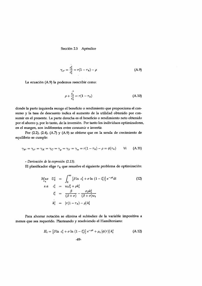
Sección 2.5 Apéndice
r('l - Tfc) - p (A.9)
La ecuación (A.9) la podemos reescribir como:
. %
P + ~i = r (1 - Tk)ct(A.10)
donde la parte izquierda recoge el beneficio o rendimiento que proporciona el consumo y la tasa de descuento indica el aumento de la utilidad obtenido por consumir en el presente. La parte derecha es el beneficio o rendimiento neto obtenido por el ahorro y, por lo tanto, de la inversión. Por tanto los individuos optimizadores, en el margen, son indiferentes entre consumir e invertir.
Por (2.2), (2.4), (A.7) y (A.9) se obtiene que en la senda de crecimiento de equilibrio se cumple:
7 fci = 7c* = l K = 1 C = l g = l Y = l w = r(! - T k) - P = Vi (A.ll)
- Derivación de la expresión (2.13).El planificador elige T). que resuelve el siguiente problema de optimización:
Para ahorrar notación se elimina el subíndice de la variable impositiva a menos que sea requerido. Planteando y resolviendo el Hamiltoniano:
M ax (12)
s.a q.c{ = wtl\ + pk\ ji P <?PkÍ
(0 + a) (0 + cr)wt
k\ = [r(l - Tfc) - p] k¡
Ht = [0 ln c¡ + a ln (1 - l\)\ e~pt + pt [0(r)] k\ (A.12)
-49-
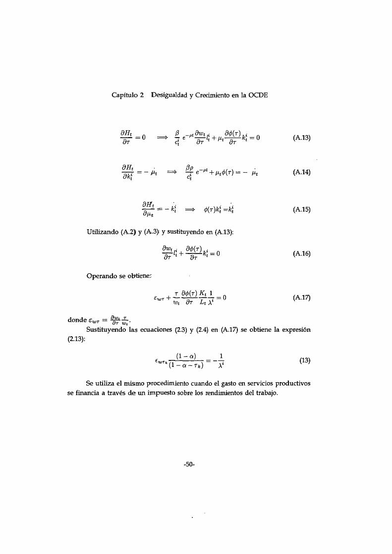
Capítulo 2 Desigualdad y Crecimiento en la OCDE
dHtdr = 0 J. e Lt + H'tdr dr (A.13)
dHtd k í
= - i h É E r - p t (A.14)
fln r^ = - k lt = » ( ¡ ) { T ) k \ = k \ (A.15)
Utilizando (A.2) y (A.3)i y sustituyendo en (A.13):
dwt ■ dó(r)- ^ + - § ^ = 0 (A.16)
Operando se obtiene::
T d ( j > { T ) K t l
emT + ^ ~ L t y - ° (A17)
donde e „ T =Sustituyendo la;s ecuaciones (2.3) y (2.4) en (A.l7) se obtiene la expresión
(2.13):
e — (* ~ a ) L (1 3 )WTfc( i - a - T k) - y
Se utiliza el mismo procedimiento cuando el gasto en servicios productivos se financia a través de un impuesto sobre los rendimientos del trabajo.
-50-

Chapter 3 Human Capital Inequality and Economic Growth
3.1 IntroductionHow is inequality generated? How does inequality evolve over time? How does inequality influence other variables such as economic growth? Numerous researchers have tried to answer these questions over the years. Initially, economists paid at- tention to factors that determine income inequality as, for example, in the influ- ential work of Kuznets (1955), who analyzed the effects of economic development upon the evolution of the distribution of income. In contrast, more recent literature addresses the question of how income or wealth distribution affects the growth of income, that is, it focuses on the potential effects of inequality on economic growth through different channels.
In spite of the distribution of wealth being the relevant inequality source in theoretical models, the scarcity of available data on the distribution of wealth for a broad number of countries and for sufficiently long periods leads most empirical studies to use income inequality data as a proxy for wealth inequality.1 On other occasions, the distribution of wealth is proxied by the distribution of land. For example, Alesina and Rodrik (1994) and Deininger and Squire (1998) include land inequality along with income inequality to analyze the relationship between initial inequality in the asset distribution and long-term growth.
However, income and land inequality may be insufficient measures of wealth inequality since other variables such as human capital are also im portant determi- nants of wealth and growth. Thus, in some models that analyze the relationship between inequality and economic growth, the role played by hum an capital en- dowment is very important if not crucial, since the distribution of income is mainly given by the distribution of hum an capital. For instance, Glomm and Ravikumar (1992), Saint-Paul and Verdier (1993) or Galor and Tsiddon (1997), among others, present models in which the source of inequality is mainly determined by the dis-
1 Measures of income inequality in growth regressions have been used by Persson and Tabellini (1994), Clarke (1995), Perotti (1996), Barro (2000), Forbes (2000) or Benerjee and Duflo (2000), among others.
-51-

Chapter 3 Human Capital Inequality and Economic Growth
tribution of hum an capital. But, at the same time, inequality affects hum an capital accumulation. In fact, some of the more interesting theories of how inequality affects growth (e.g., Galor and Zeira, 1993) are based on the interaction between imperfect credit markets, asset inequality and human capital accumulation.
The interest in these mechanisms at the theoretical level contrasts with the scarcity of empirical results. Due to the lack of available data on hum an capital inequality, little attention has been devoted to the influence of hum an capital distribution on economic growth in empirical studies. Some exceptions are Birdsall and Londoño (1997), and López, Thomas and Wang (1998). Using a sample of 43 countries, Birdsall and Londoño (1997) analyze the effect of initial inequalities in the distribution of income, land and hum an capital on economic growth. They obtain a negative effect from initial land and education inequality on aggregate growth. Moreover, this negative effect is stronger when the dependent variable is the income growth rate of the poorest. Nevertheless, in this paper, whereas income and land inequality are measured by a Gini coefficient, education inequality is measured by the standard deviation of years of education. The problem with the standard deviation, however, is that it is an absolute measure of dispersión thus it does not control for differences in the mean of the distribution.
López, Thomas and Wang (1998) use a panel data for 12 Asian and Latín American countries from 1970 to 1994. They analyse the effects of average education and education distribution on per capita income and on economic growth. They show that hum an capital inequality, measured by the coefficient of variability of education and the standard deviation of the log of education, has had a negative impact on per capita income in most countries. On the other hand, although their results indícate that the positive effect of education on economic growth is greater under competitive and open market conditions, in their regressions there is no ev- idence of a negative and significant effect of human capital inequality, measured by the coefficient of variability, on economic growth.
The objective of this chapter is to provide new hum an capital inequality measures, that allow us to make a first approximatíon of the relationship between these indicators and economic growth in a broad number of countries. In particular, using the recent Information contained in Barro and Lee's (2001) data set about educational attainments, we calcúlate a hum an capital Gini coefficient. Addition- ally, to improve the information provided by this aggregate measure of inequality, we also compute the distribution of education by quintiles, in line with a number of contributions to the analysis of the relationship between the distribution of
-52-

Section 3.2 Measuring Human Capital Inequality
income and economic growth.Apart from their intrinsic interest, an additional advantage of our indica-
tors is that they conveniently complement the information provided by income inequality measures. Clearly, income distribution data suffer from several prob- lems. Besides the limitations related to their quality, the main problem arises with the different definitions of income used to measure inequality.2 Although the income distribution data set of Deininger and Squire (1996) has represented a sig- nificant improvement in coverage and quality compared with previous data sets, there is room for improvement in other inequality indicators, especially in devel- oping countries where income inequality data are more scarce. O ur measures of hum an capital inequality are only restricted by the coverage and quality of Barro and Lee's figures, which refer to 108 countries over five-year intervals from 1960 to 2000.3
O ur new measures of hum an capital inequality allow us to have a closer look at the relationship between inequality and economic growth. The main find- ings illustrate that hum an capital inequality measures provide more robust results than income inequality measures in the growth regressions. Moreover, the results suggest that hum an capital inequality negatively influences economic growth rates not only through the efficiency of resource allocation but also through a reduction in investment rates.
The structure of this chapter is as follows. Section 3.2 presents the procedure used to obtain the Gini index and the distribution of education by quintiles, and it compares the information provided by these different measures. Section 3.3 an- alyzes the distribution of the hum an capital inequality indicators across countries and their evolution from 1960 to 2000. Section 3.4 presents preliminary evidence on the relationship between our measures of hum an capital distribution and other indicators of development. Section 3.5 studies the relationship between hum an capital inequality and economic growth. Finally, Section 3.6 contains the conclusions reached.
2 The three main differences in these definitions are given by the distinction between gross and net income, income and expenditure and, finally, per capita and household income.3 The last Barro and Lees (2001) data set improve on their earlier data sets (Barro and Lee (1993), Barro and Lee (1996)). In particular, they have revised their fill in procedure to use 'adjusted gross enrollment ratios1, they have taken account of changes in the duration of schooling within countries and they have update their earlier data set up to 2000.
-53-

Chapter 3 Human Capital Inequality and Economic Growth
3.2 Measuring Human Capital InequalityThis section describes how we have obtained the measures of hum an capital inequality for a broad cross section of countries. We take schooling figures from Barro and Lee (2001) to construct a standard representation of inequality such as the Gini coefficient. The choice of this index to analyze inequality in the distribution of hum an capital is mainly due to the fact that it is the one normally used in intemational comparisons of income distribution. Nevertheless, as pointed out by Deininger and Squire (1996) among others, it is difficult to characterize inequality by such a simple measure. For this reason, to extend the information provided by the Gini index we also report figures of the distribution of education by quintiles.
There are different ways of computing the Gini coefficient. Since the Barro and Lee's data set provides information of the average schooling years and attain- ment levels, the hum an capital Gini coefficient (Gh) can be computed as follows:4
j 3 3
G k = 2 H ^ ~~ ^ I niTli (31>i=0 j = 0
where H are the average schooling years of the population aged 15 years and over, i and j stand for the different levels of education, n¿ and rij are the shares of population with a given level of education, and Xi and Xj are the cumulative average schooling years of each educational level. Following Barro and Lee (2001), we consider four levels of education: no schooling (0), primary (1), secondary (2) and higher education (3). Defining Xi as the average schooling years of each educational level i, we observe that5
XQ = X 0 = 0, Xi = X \, X2 = X \-\- X2, X3 = X\ + X2 + X3 (3.2)
Expanding expression (3.1) and using (3.2), the Gini coefficient can be computed
4 This expression has also been used in two recent papers by Thomas, Wang and Fan (2000) and Checchi (2000) to obtain a human capital Gini coefficient. In contrast with our approach, Checchi (2000) uses the information of the education for the population aged 25 years and over. For many developing countries a large portion of the labor forcé is younger than 25. Since most of our sample is composed of developing countries, we have used the educational information for the population aged 15 and over.5 In terms of the variables of Barro and Lee's data set, we have that xo — 0, x \ = pyr l5 / ( lp l5+l s l5 +lh l5 ) , xz = syrl5/ ( ls l5+lhl5), X3 = hyrl5/ lhl5, no = lulb, ni = lpl5, ri2 = lsl5, ri3 = lhl5 and H = tyr 15.
-54-

Section 3.2 Measuring Human Capital Inequality
as follows:
Wi _ , n i x 2(n2 + n 3) + n s x ^ + n 2)Lr = no H---------------- 7---------- r 7-------------------- r (3.3)
n iX i + ri2 \x i + X2 ) + n z{x i + x 2 + £ 3 )
Besides the Gini coefficient, Barro and Lee's data set can also be used toobtain the distribution of education by quintiles. Table 3.1 shows two examplesthat illustrate how these measures have been obtained for two countries which are at opposite extremes of the distribution. A good example of a large concentration of education, with a Gini coefficient cióse to one, is Yemen in 1975. In this country 98.8% of the population had no schooling. This means that, in terms of quintiles, the first four quintiles have no education, and all education is concentrated in the top quintile. On the contrary, a Gini coefficient cióse to zero would represent the case where the attainment level in each quintile is similar. A good example is the United States in 1980 where the share of total education attained by each quintile is around 0 .2 .
Although Barro and Lee's data set is the best available source on hum an capital stocks for a large sample of countries to date, as Krueger and Lindahl (2001) or De la Fuente and Doménech (2001) have pointed out, the measurement errors for different education levels, due to the poor quality of the original sources, can be particularly substantial in some countries. To the extent that we use Barro and Lee's data set, we acknowledge the presence of some measurement errors which may distort the inequality variables we have computed.
Basic descriptive statistics of the Gini coefficients and the distribution of education by quintiles are shown in Table 3.2. All countries for which hum an capital variables are available have been classified in seven different groups: M iddle East and North Africa, Sub-Saharan Africa, Latín America and the Caribbean, East Asia and the Pacific, South Asia, Advanced Countries and Transitional Economies. The data sets includes 108 countries in the world from 1960 to 2000, there is a total of 935 observations.
The second column of Table 3.2 (G h) illustrates that South Asia countries are the group that, on average, have the largest hum an capital Gini coefficient (0.697). On the contrary, the countries with a more egalitarian distribution of hum an capital are the Advanced Countries with a mean of 0.208. The countries in the north of Europe as well as Australia, Cañada, New Zealand and the United States have the lowest Gini coefficients.6 With regard to the quintiles, the third column shows
6 See Appendix 2 for average country data.
-55-

Chapter 3 Human Capital Inequality and Economic Growth
Table 3.1Two examples of the distribution of education by quintiles
Education levels Quintilesi Xi rii s Ps Ps x s u s Qs G h
Yemen 0 0 0.988 1 0.20 0.20 0 0 0 0.990(1975) 1 5.2 0.005 2 0.20 0.40 0 0 0
2 4.5 0.005 3 0.20 0.60 0 0 03 2.0 0.001 4 0.20 0.80 0 0 0
5 0.20 1.00 0.098 0.098 1.0
United 0 0 0.009 1 0.20 0.20 1.898 1.898 0.161 0.080States 1 5.9 0.051 2 0.20 0.40 2.279 4.176 0.353(1980) 2 5.5 0.662 3 0.20 0.60 2.279 6.455 0.546
3 2.9 0.281 4 0.20 0.80 2.506 8.961 0.7585 0.20 1.00 2.861 11.822 1.000
Definitions: i is the education level (no schooling (0), primary (1), secondary (2) and tertiary (3)), X{ is the average schooling years of each educational level, is the share of no schooling, primary, secondary and higher schooling attained by the population aged 15 years and over, s is the quintile, p s is the share of the population in each of the fíve intervals, p s is the cumulative population share,
Sx s is the total schooling years attained by each of the quintiles, u s= ^ x m and
m= lthe cumulative share of education attained by each quintile is Q s=us/ u 5 . As an example, in the case of the United States in 1980, since no + n i < 0 .2 , the total schooling years attained by the first quintile ( í i ) is given by x \ = nQXo + n \X \ +(0.20 - ni - n o ) ( x i + X 2 ) = 1.898
that the ranking among countries in terms of human capital equality, measured by the third quintile (Q 3 ), is equal to the one obtained with the Gini coefficient. How- ever, the order differs with the ratio of the bottom quintile to the top one (column 4). Although South Asia countries show on average a larger Gini coefficient than Sub-Saharan African countries, the low est 20% of the population receives more education in the former group than in the latter. As a result, South Asia is the región with the greatest inequality, measured by the Gini coefficient, whereas Sub Sahar- ian Africa is the región with the greatest inequality, measured by the ratio of the bottom to the top quintile.
The fifth column indicates that all groups of countries, with the exception of Advanced Countries, have decreased the inequality in the distribution of human
56-
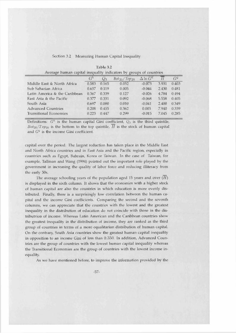
Section 3.2 Measuring Human Capital Inequality
Table 3.2Average human capital inequality indicators by groups of countries
G h Q s Bot 20 /T o P20 A ln G h H G yM iddle East & North Africa 0.583 0.165 0.032 -0.073 3.931 0.403Sub Saharian Africa 0.637 0.119 0.005 -0.044 2.430 0.481Latin America & the Caribbean 0.367 0.339 0.127 -0.026 4.784 0.494East Asia & the Pacific 0.377 0.331 0.092 -0.068 5.558 0.405South Asia 0.697 0.080 0.010 -0.041 2.400 0.349Advanced Countries 0.208 0.455 0.362 0.003 7.940 0.339Transitional Economies 0.223 0.447 0.299 -0.015 7.045 0.285
Definitions: G h is the human capital Gini coefficient, Qz is the third quintile, B o t2o /T o p 2o is the bottom to the top quintile, H is the stock of human capital and Gy is the income Gini coefficient.
capital over the period. The largest reduction has taken place in the M iddle East and North Africa countries and in East Asia and the Pacific región, especially in countries such as Egypt, Bahrain, Korea or Taiwan. In the case of Taiwan, for example, Tallman and Wang (1994) pointed out the important role played by the governm ent in increasing the quality of labor forcé and reducing illiteracy from the early 50s.
The average schooling years of the population aged 15 years and over (H ) is displayed in the sixth column. It shows that the economies with a higher stock of human capital are also the countries in which education is more evenly dis- tributed. Finally, there is a surprisingly low correlation between the human capital and the income Gini coefficients. Comparing the second and the seventh columns, w e can appreciate that the countries with the low est and the greatest inequality in the distribution of education do not coincide with those in the dis- tributrion of income. Whereas Latin American and the Caribbean countries show the greatest inequality in the distribution of income, they are ranked as the third group of countries in terms of a more equalitarian distribution of human capital. On the contrary, South Asia countries show the greatest human capital inequality in opposition to an income Gini of less than 0.350. In addition, Advanced Countries are the group of countries with the low est human capital inequality whereas the Transitional Economies are the group of countries with the low est income inequality.
As w e have mentioned before, to improve the information provided by the
-57-

Chapter 3 Human Capital Inequality and Economic Growth
Gini coefficient, we have also computed the distribution of education by quintiles, in line with some of the most recent contributions to the analysis of the relationship between the distribution of income and economic growth. For instance, Persson and Tabellini (1994) use the third quintile as a measure of equality, Perotti (1996) combines the third and fourth quintile to capture the notion of "m iddle class", and Deininger and Squire (1996) calcúlate the top to the bottom quintile ratio as a measure of inequality.
The correlations between different measures of human capital inequality are displayed in Table 3.3. The table shows a strong negative correlation between the Gini index and the different quintiles. The correlation is greater than 0.9 between the Gini index and the second, third and fourth quintiles. In particular, the greatest correlation is with the third quintile with a coefficient cióse to one, whereas the quintile with the smallest correlation is the first one. The indicator of equality, the ratio of the bottom quintile to the top one (x \ / x 5), is the measure with the lowest correlation, although it is still very high in absolute terms. These results reveal that the hum an capital Gini coefficient seems to be a good indicator of the education attained by the 60 per cent of the population. However, to analyse what happens in the tails of the distribution, it would be better to use the first and fifth quintiles directly or a combination of them.
In spite of the high correlation between the Gini coefficient and the different quintiles, changes from 1960 to 2000 in the Gini coefficient may be associated with different movements in quintiles. Thus, to get additional information that is not captured by the aggregate measure of inequality, Table 3.4 shows educational shares of the lowest, middle and highest quintiles by groups of countries during the period 1960 to 2000.
In Table 3.4 we can observe some examples that illustrate the valué of com- bining the aggregate measure of inequality and information on educational shares. For instance, South Asia countries show, on average, a larger Gini coefficient than Sub-Saharan African countries, since the third quintile is greater in the latter group. However, the lowest 20 per cent of the population receive more education in South Asian countries than in Sub-Saharan African región. In addition, looking at the Gini coefficient, there is a small difference between the Gini index of Latin Amer-
7 Deininger and Squire (1996) compute the Top20/Bottom20 ratio as a measure of income inequality. Nevertheless, as many countries have a high percentage of illiterates, to avoid divisions by zero, we compuete the inverse of this ratio, which can be interpreted as a measure of equality.
-58-
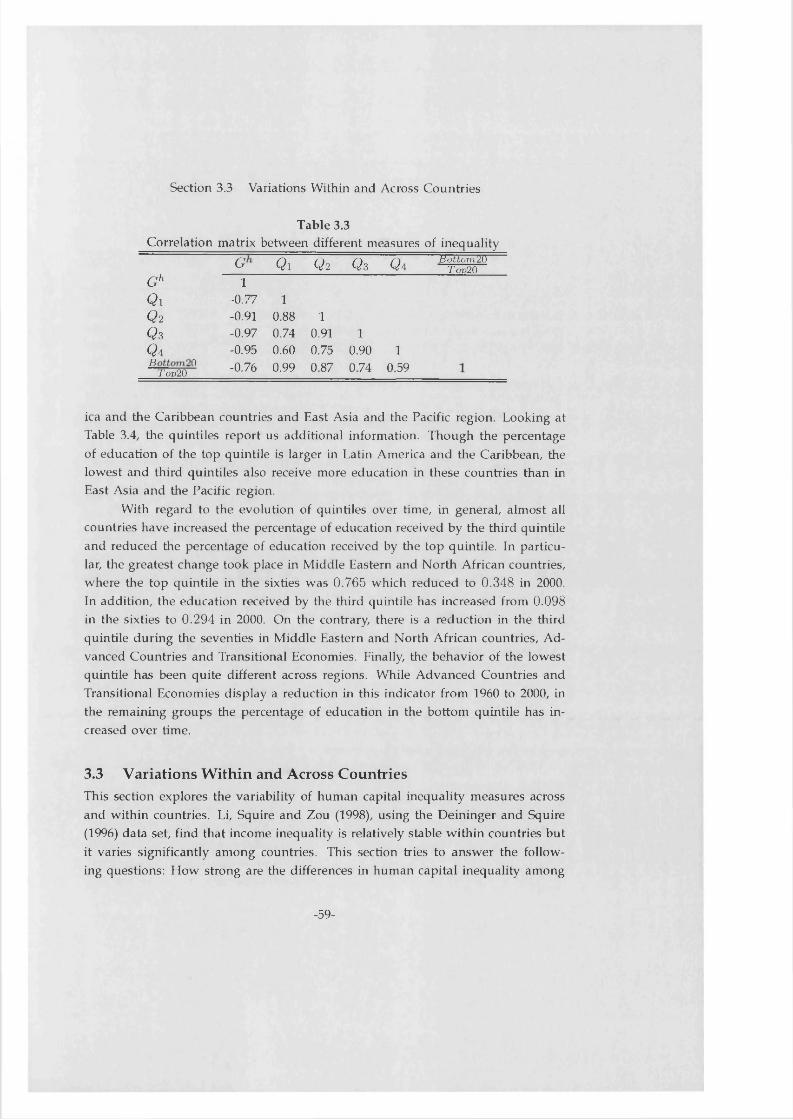
Section 3.3 Variations Within and Across Countries
Table 3.3Correlation matrix between different measures of inequality
tlottomTJOT op2 0O Q i Q 2 Q 3 Qa
G h 1Q i -0.77 1Q 2 -0.91 0.88 1(¿3 -0.97 0.74 0.91 1<¿4 -0.95 0.60 0.75 0.90 1
PTw20° ~°-76 ° " 0 87 0 74 0 59
ica and the Caribbean countries and East Asia and the Pacific región. Looking at Table 3.4, the quintiles report us additional information. Though the percentage of education of the top quintile is larger in Latin America and the Caribbean, the lowest and third quintiles also receive more education in these countries than in East Asia and the Pacific región.
With regard to the evolution of quintiles over time, in general, alm ost all countries have increased the percentage of education received by the third quintile and reduced the percentage of education received by the top quintile. In particular, the greatest change took place in Middle Eastem and North African countries, where the top quintile in the sixties was 0.765 which reduced to 0.348 in 2000. In addition, the education received by the third quintile has increased from 0.098 in the sixties to 0 .294 in 2000. On the contrary, there is a reduction in the third quintile during the seventies in M iddle Eastern and North African countries, Advanced Countries and Transitional Economies. Finally, the behavior of the lowest quintile has been quite different across regions. While Advanced Countries and Transitional Economies display a reduction in this indicator from 1960 to 2000, in the remaining groups the percentage of education in the bottom quintile has increased over time.
3.3 V a r ia t io n s W ith in a n d A c ro ss C o u n tr ie sThis section explores the variability of human capital inequality measures across and within countries. Li, Squire and Zou (1998), using the Deininger and Squire (1996) data set, find that income inequality is relatively stable within countries but it varíes significantly among countries. This section tries to answer the foliow- ing questions: H ow strong are the differences in human capital inequality among
-59-
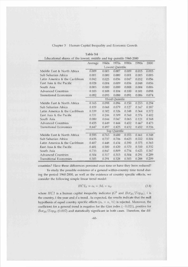
Chapter 3 Human Capital Inequality and Economic Growth
Table 3.4Educational shares of the lowest, middle and top quintile 1960-2000
Average 1960s 1970s 1980s Lowest Quintile
1990s 2000
Middle East & North Africa 0.009 0.003 0.007 0.009 0.015 0.015Sub Saharian Africa 0.001 0.000 0.000 0.001 0.003 0.005Latin America & the Caribbean 0.042 0.025 0.036 0.047 0.052 0.056East Asia & the Pacific 0.028 0.004 0.009 0.036 0.048 0.056South Asia 0.003 0.000 0.000 0.008 0.004 0.006Advanced Countries 0.103 0.108 0.104 0.100 0.101 0.098Transitional Economies 0.082 0.095 0.080 0.091 0.086 0.074
Third QuintileMiddle East & North Africa 0.165 0.098 0.096 0.150 0.253 0.294Sub Saharian Africa 0.119 0.068 0.079 0.127 0.167 0.187Latin America & the Caribbean 0.339 0.302 0.326 0.348 0.364 0.372East Asia & the Pacific 0.331 0.244 0.309 0.360 0.376 0.402South Asia 0.080 0.044 0.047 0.065 0.121 0.168Advanced Countries 0.455 0.449 0.444 0.452 0.467 0.473Transitional Economies 0.447 0.497 0.425 0.432 0.452 0.356
Top QuintileMiddle East & North Africa 0.593 0.765 0.680 0.555 0.461 0.348Sub Saharian Africa 0.635 0.737 0.706 0.623 0.552 0.504Latin America & the Caribbean 0.407 0.448 0.434 0.390 0.375 0.365East Asia & the Pacific 0.401 0.500 0.420 0.370 0.350 0.332South Asia 0.733 0.847 0.809 0.734 0.625 0.567Advanced Countries 0.304 0.317 0.313 0.304 0.291 0.289Transitional Economies 0.303 0.291 0.328 0.303 0.288 0.209
countries? Have these differences persisted over time or have they been reduced?To study the possible existence of a general within-country time trend dur-
ing the period 1960-2000, as well as the existence of country specific effects, we consider the foliowing sim ple linear trend model:
HCIit — ocí 4* ¡3dt + un (3-4)
where H C I is a human capital inequality indicator (G h and B ot2o /T op2o), i is the country, t the year and d a trend. As expected, the results indica te that the nuil hypothesis of equal country specific effects (c*¿ = a , Vi) is rejected. Moreover, the coefficient for a general trend is negative for the Gini index (—0.021), positive for B o t 2o /T o p 2o (0.007) and statistically significant in both cases. Therefore, the dif-
-60-

Section 3.3 Variations Within and Across Countries
2.32000
1960
1970
1980
19900
0 0.2 0.4 0.6 0.8
Figure 3.1: Density functions of the Gini coefficient 1960-2000.
ferences in the distribution of education across countries are substantial and, in general, countries have tended to reduce the inequality in hum an capital distribution over the period under study.
The preceding exercise show s how the mean of these indicators has evolved over time, but w e also w ant to analyze how the dispersión and relative position of each country has changed from 1960 to 2000. The easiest w ay to test the con- stancy in the dispersión of the Gini coefficient is through a time plot of its standard deviation. Nevertheless, the standard deviation is not enough to characterize the distribution w hen it is not a normal one. In particular, the Bera-Jarque test re- jects the nuil hypothesis of normality of the distribution of the Gini coefficient and the ratio of the bottom to the top quintile. For this reason, in Figure 1 w e have represented the non-parametric estimation of the density functions of G h using a truncated gaussian kernel for a distribution in the interval [0,1]. As w e can see,
8 We thank F. J. Goerlich for providing the programme that implements such a procedure. The main result shown in Figure 3.1 is robust to changes in bandwith parameters.
-61-
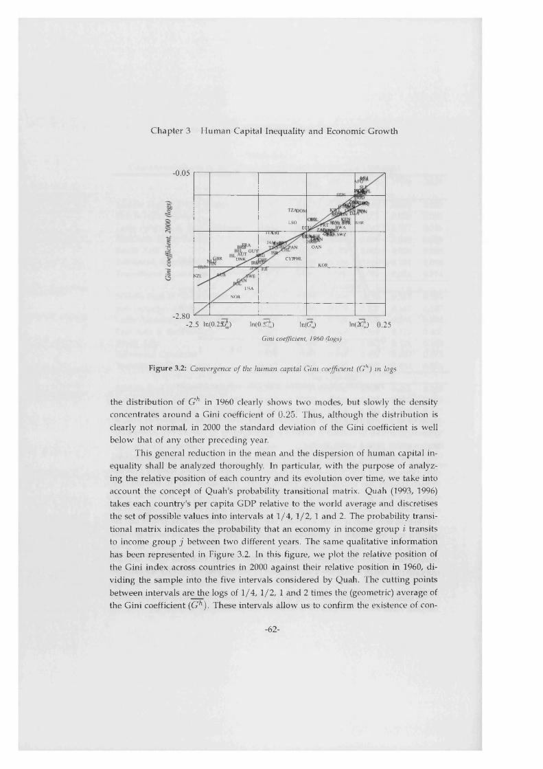
Chapter 3 Human Capital Inequality and Economic Growth
-0.05
LSO SHR,ftWAE( l,SWZ
JAIOAN
¡BR D N K ^ < CYH’HLKOR
MZL
USA
ÑOR
-2.80-2.5 ln(0.25tf) ln(0.3Ct) ln(G^) ln(2g£) 0.25
Gini coefficient, 1960 (logs)
Figure 3.2: Convergence of the human capital Gini coefficient (Gh) in logs
the distribution of G h in 1960 clearly shows two modes, but slowly the density concentrates around a Gini coefficient of 0.25. Thus, although the distribution is clearly not normal, in 2000 the standard deviation of the Gini coefficient is well below that of any other preceding year.
This general reduction in the mean and the dispersión of human capital inequality shall be analyzed thoroughly. In particular, with the purpose of analyz- ing the relative position of each country and its evolution over time, we take into account the concept of Quah's probability transitional matrix. Quah (1993, 1996) takes each country's per capita GDP relative to the world average and discretises the set of possible valúes into intervals at 1 /4 ,1 /2 ,1 and 2. The probability transitional matrix indicates the probability that an economy in income group i transits to income group j between two different years. The same qualitative information has been represented in Figure 3.2. In this figure, w e plot the relative position of the Gini index across countries in 2000 against their relative position in 1960, di- viding the sample into the five intervals considered by Quah. The cutting points between intervals are the logs of 1 / 4 , 1 / 2 , 1 and 2 times the (geometric) average of the Gini coefficient (G h). These intervals allow us to confirm the existence of con-
-62-
Section 3.4 Correlation between human capital inequality and other indicators of development
vergence or polarisation of the Gini coefficient. If countries had converged, they should have changed from their initial intervals in 1960 to the one around the average in 2000. On the contrary, if there had been a polarisation in hum an capital Gini coefficients, countries should have changed from their initial intervals to the extremes. The diagonal simply reflects thé logs of the Valúes of the Gini index in 1960 multiplied by the sample average rate of growth between 1960 and 2000. Thus, countries win or lose in relative positions according to their vertical distance to the diagonal. As we can see in Figure 3.2, some countries that showed a high inequality in 1960 (that were in the fifth interval) have reduced inequality, moving to the fourth interval by 2000. Likewise, some countries that were in the fourth interval in 1960 have reduced inequality, moving to the third interval by 2000, as in the case of Korea, Taiwan and Hong Kong, which are good examples of an important reduction in hum an capital inequality. On the contrary, some OECD countries have worsened their relative positions changing to higher intervals by 2000.
Finally, Figure 3.2 also shows the adjusted valúes of the Gini index in 2000 after estimating an equation where the Gini index in 1960 is the regressor, both in logs. The smaller the slope of the adjusted line, the bigger the convergence process is. As we observe in this figure, it seems that during the period 1960 to 2000 there has been a process of convergence in the valúes of the Gini coefficients since the slope of the regression line is smaller than the slope of the diagonal line (the estimated coefficient is equal to 0.673 with a t —ratio equal to 16.49).
3.4 Correlation between human capital inequality and other indicators of development
This section provides some additional empirical evidence about the relationship between hum an capital inequality, measured through the Gini coefficient (Gh) and the quintiles (Q i, Q 2 , Qz, Qa) and other indicators of development such as the level of GDP per capita (y), the stock of hum an capital (H), hum an capital accumulation (Sh), life expectancy (LE), population growth (n), income inequality (Gy), the ratio of govemment expenditure on education to GDP (s^), the investment rate (Sk) or the ratio of govemment consumption to GDP (g).
-63-

Chapter 3 Human Capital Inequality and Economic Growth
Table 3.5Correlation Matrix of different indicators of development
Gh H Sh LE y n a9s h 9 Sk GyGh 1 .0 0
H -0 .9 0 1 .0 0
(9 3 5 )
Sh -0 .7 6 0 .8 6 1 .0 0(6 08) (6 08)
L E -0 .8 7 0 .8 6 0 .8 8 1 .00(5 87) (5 87) (603)
y -0 .6 8 0 .8 2 0.81 0 .76 1 .0 0
(6 77) (6 7 7 ) (606) (595)
n 0 .5 4 -0 .5 8 -0 .5 5 -0 .51 -0 .6 3 1 .0 0
(5 01) (5 0 1 ) (5 20) (503) (506)
bh -0 .3 6 0 .4 6 0 .4 9 0 .40 0 .4 7 -0 .2 7 1.00
(4 57) (4 5 7 ) (4 70) (461) (462) (4 72)
9 0 .4 2 -0 .3 7 -0 .3 0 -0 .41 -0 .3 7 0 .2 5 0.18 1 .0 0(5 9 5 ) (5 9 5 ) (610) (599) (614) (5 09) (464)
Sk -0 .6 6 0 .6 4 0 .6 4 0 .69 0 .5 8 -0 .4 6 0 .34 -0 .3 8 1 .0 0
(5 9 5 ) (5 9 5 ) (610) (599) (614) (509) (464) (618)
G y 0 .2 7 -0 .4 3 -0 .4 9 -0 .2 7 -0 .4 0 0 .5 3 -0 .25 -0 .01 -0 .3 4 1 .0 0
(2 9 7 ) (2 9 7 ) (237) (238) (287) (180) (172) (235) (235)
Q i -0 .7 7 0 .7 9 0 .7 3 0 .70 0.71 -0 .6 4 0 .44 -0 .31 0 .5 3 -0 .4 6
(9 35) (9 3 5 ) (608) (587) (677) (501) (457) (595) (595) (2 9 7 )
Q2 -0 .91 0 .8 6 0 .7 5 0 .82 0 .6 8 -0 .6 5 0 .36 -0 .3 7 0 .5 9 -0 .31
(9 3 5 ) (9 3 5 ) (608) (587) (677) (501) (457) (595) (595) (2 97)
Qs -0 .9 7 0 .8 8 0 .7 2 0 .84 0 .6 4 -0 .5 6 0.33 -0 .41 0 .6 4 -0 .21
(9 3 5 ) (9 3 5 ) (608) (587) (677) (501) (457) (595) (595) (2 97)
Q a -0 .9 5 0 .8 2 0 .6 7 0 .80 0 .5 6 -0 .41 0.31 -0 .41 0 .6 2 -0 .1 8
(9 3 5 ) (9 3 5 ) (608) (587) (677) (501) (457) (595) (595) (2 97)
Note- The number of observations is in parenthesis.
From Table 3.5, which contains the correlation matrix between the variables under consideration, we can observe the foliowing results:
1. There is a strong negative relationship between the Gini index and the stock of human capital (H ), measured as the average years of schooling in the total population. In fact, the correlation between Gh and H is very high (—0.90).
-64-

Section 3.4 Correlation between human capital inequality and other indicators of development
India
Indonesia
0 0.2 0.4 0.6 0.8 1Human Capital Gini Coefficient
Figure 3.3: Human capital inec¡uality and the level of human capital (average years of schooling).
This suggests that the econom ies with a higher stock of human capital are also the countries in which education is more evenly distributed. However, Figure 3.3 show s that the dispersión among both indicators increases substantially as the Gini index falls. We also find many countries that, in spite of having the same average schooling years, significantly differ in the distribution of education. According to recent World Bank figures, in the 80's India and Indonesia, both highly populated countries, had similar levels of income inequality. They also had similar levels of average years of schooling: approximately 3.6 years of formal education. However, as Figure 3.3 shows, the distribution of education was quite different since the proportion of the population with no schooling and, at the other extreme, with a university education was much higher in India than in Indonesia.
2. Similarly, there is a strong relationship between the Gini index and the life ex- pectancy (LE). The countries with a more equalitarian distribution of human capital are those in which their citizens, on average, live longer. The countries
-65-

Chapter 3 Human Capital Inequality and Economic Growth
with life expectancy around 70 years oíd are the countries with the best distribution in hum an capital whereas the countries with Gini coefficients next to one have a life expectancy less than 50 years oíd. For example, in 1960, both Mali and Niger had a hum an capital Gini coefficient of 0.948 and a life expectancy of 35.9 and 35.4 years oíd, respectively. In opposition, in the same year, some Advanced Countries such as Norway, The Netherlands or Switzerland had a life expectancy of 73.4, 73.3 and 73.2 years oíd, respectively, and a hum an capital Gini coeffcient lower than 0.2.
3. There is a negative correlation between the Gini index and the govemment ex- penditure on education (sgh). Although the correlation is not too high, this negative sign m ay suggest that the societies with less inequality in hum an capital are those in which their govemments spend more on education.
4. Countries with the greatest income per capita (y) are also the countries with the best distribution in hum an capital. This negative correlation also applies with the investment rate (Sk).
5. There is a positive correlation between the hum an capital Gini coefficient and the population growth rate (n).
6. Income Gini coefficient (Gy) and hum an capital Gini coefficient are correlated positively. Nevertheless, this coefficient is not too high (0.27). As we pointed out in section two, the group of countries with the greatest inequality in the distribution of income (Latin America and the Caribbean) does not coincide with the group of countries with the greatest inequality in the distribution of hum an capital (South Asia). Likewise, the group of countries with the lowest inequality in the distribution of income (Transitional Economies) does not coincide with the group of countries with the lowest inequality in the distribution of hum an capital (Advanced Countries). Moreover, Figure 3.4 suggests a non linear relationship between income inequality and hum an capital inequality.
7. With regard to the quintiles, due to the high correlation between the human capital Gini coefficient and the different quintiles, most of the results obtained with the Gini coefficient hold with the quintiles. However, some results must be remarked. First, the greatest correlation between per capita income and the different quintiles appears with the first one. On the contrary, the first quintile is the one that shows the lowest correlation with the physical capital investment rate. Second, the population growth rate is more correlated with the lowest quintiles (first and second) than with the highest (third and fourth). Third, the greatest positive correlation between the public spending on education and the
-66-

Section 3.5 Human Capital Inequality and Economic Growth
0 .7
•i» • *
0 .3
0.20 0.2 0 .4 0.6 0.8 1
Human Capital Gini Coefficient
Figure 3.4: Income inequality and human capital inequality.
quintiles appears with the first one. This could indicate that public spending on education benefits mainly the share of population with the low est education. Finally, the last column indicates that income inequality is more correlated with the share of education of the bottom 20 per cent of the population than with the share of education of the higher quintiles.To sum up, w e have seen that human capital inequality and the stock of hu
man capital are strongly and negatively correlated and that the stock of human capital is negatively correlated with income inequality. Moreover, the countries with more expenditure on education are also the countries with less inequality in human capital. Thus, these correlations suggest that universal education could reduce human capital inequality and increase the stock of education, which could transíate into a reduction in income inequality. Nevertheless, more evidence on these relations is needed.
-67-

Chapter 3 Human Capital Inequality and Economic Growth
3.5 Human Capital Inequality and Economic GrowthIn this section, we focus on the effect that human capital inequality can exert on economic growth rates. To consider this issue, we add inequality variables to an equation where the average economic growth is explained by initial per capita income and the average accumulation rates of human and physical capital. Next, we increase the set of explanatory variables to prove the robustness of the initial results. Finally, we repeat the exercises with different samples.
The results of this section should be seen as a first attempt to evalúate the effects of hum an capital inequality upon economic growth using these measures rather than as a defmitive analysis of the determinants of growth or as a test of any particular model. Additionally, although we are aware of some recent devel- opments in the econometric analysis of economic growth and convergence, such as the contributions of Islam (1995), Caselli, Esquivel and Lefort (1996), and Lee, Pesaran and Smith (1997,1998), our approach relies deliberately on standard cross- section and pooling regressions in order to facilitate the comparison with previous results in related literature.9
The data used in our growth regressions comes from Barro and Lee (1994,2001) with the exception of the variables concerning inequality. With regard toincome inequality, G y is proxied by Deininger and Squire's (1996) high qualityincome Gini coefficient. Although we would like to include this variable at thebeginning of the period (cióse to 1960), the problems with the availability of high
10quality income Gini data restrict us to including this variable as an average.In our initial regression, shown in Table 3.6, the average growth rate of per
capita income from 1960 to 1990 (A ln y) is the dependent variable and income inequality is included as an explanatory variable along with the logs of human capital accumulation (ln Sh), defined as the total gross enrollment ratio for secondary education (taken from UNESCO), physical capital accumulation (ln Sfc), defined as the ratio of real domestic investment to real GDP, the black market pre- mium {B M P ) to control for government distortions of markets, and initial per
9 For example, using panel techniques to control for time invariant country-specific effects, Forbes (2000) gets very different results of the effects of income inequality on economic growth to the ones obtained by Alesina and Rodrik (1994), Perotti (1996), Persson and Tabellini (1994), or Deininger and Squire (1998).10 The inclusión of the income Gini at the beginning of the period significantly reduces the size of the sample. As the variability of this coefficient is very low throughout the whole period (see Li, Squire and Zou (1998)) the inclusión of this variable as an average does not change the main results.
-68-

Section 3.5 Hum an Capital Inequality and Economic Growth
capita income (ln y). The results are as expected: on the one hand, the coefficients of the accumulation of factors are positive and statistically significant and,on the other, initial income per capita and income inequality coefficients are neg-
11atively and significantly related to per capita income growth. Nevertheless, this result is not robust to the inclusión of additional variables to the set of regressors. In particular, as obtained by Deininger and Squire (1998), the coefficient of Gy is not statistically significant when we include regional dummies, which capture perm anent and specific characteristics of the regions that otherwise could bias the coefficients of some explanatory variables. Moreover, when we add hum an capital inequality in 1960, measured by the hum an capital Gini coefficient (G h) in this basic growth equation, the coefficient of Gy even becomes positive, as shown in column (2), whereas the coefficient of Gh is negative and significant. These initial results suggest, therefore, that the negative relationship between income inequality and growth, obtained in previous studies, is not robust to the inclusión of other variables in the regression.
In column (3) of Table 3.6, income inequality has been excluded from the set of explanatory variables. Although our hum an inequality indicator may con- tain some m easurement errors as we have mentioned earlier, in contrast to the results for income inequality, the coefficient of hum an capital inequality is again negative and statistically significant when regional dummies are present. A similar result is obtained in column (4) when we include other explanatory variables often considered in the literature: the log of the average population growth (as in Mankiw, Romer and Weil, 1992, augmented by the rate of technical progress and the depreciation rate, assumed to be 0.02 and 0.03, respectively) and public consumption over GDP.
The preceding regressions consider the direct effect of inequality on growth, but it is also possible that inequality variables are related indirectly to economic growth through the accumulation of factors. Column (5) shows that once the rates of hum an and physical capital accumulations are ruled out from the set of explanatory variables, initial hum an capital inequality has a bigger negative effect on the economic growth rates, suggesting that the indirect effects through the accumulation rates are also very important. However, given the high correlation between hum an capital inequality and its stock, it is possible that Gh may be picking up the effect of the level of hum an capital on growth. In column (6) we test this hy-
11 A negative relationship between income inequality and growth can be found in Alesina and Rodrik (1994), Persson and Tabellini (1994), Clarke (1995) or Perotti (1996).
-69-
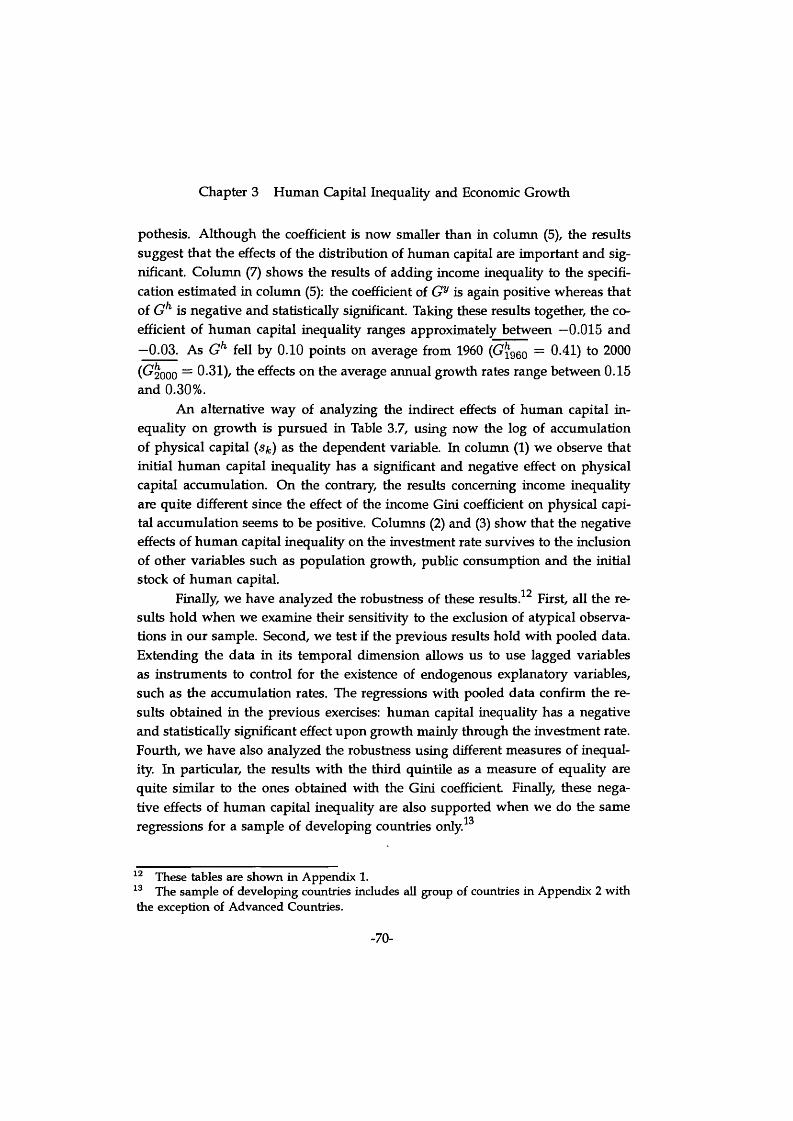
Chapter 3 Human Capital Inequality and Economic Growth
pothesis. Although the coefficient is now smaller than in column (5), the results suggest that the effects of the distribution of hum an capital are important and significant. Column (7) shows the results of adding income inequality to the specifi- cation estimated in column (5): the coefficient of Gy is again positive whereas that of Gh is negative and statistically significant. Taking these results together, the coefficient of hum an capital inequality ranges approximately between —0.015 and —0.03. As Gh fell by 0.10 points on average from 1960 (G^9q0 = 0.41) to 2000 (G2000 ” 0-31)/ the effects on the average annual growth rates range between 0.15 and 0.30%.
An alternative way of analyzing the indirect effects of hum an capital inequality on growth is pursued in Table 3.7, using now the log of accumulation of physical capital (Sk) as the dependent variable. In column (1) we observe that initial hum an capital inequality has a significant and negative effect on physical capital accumulation. On the contrary, the results conceming income inequality are quite different since the effect of the income Gini coefficient on physical capital accumulation seems to be positive. Columns (2) and (3) show that the negative effects of hum an capital inequality on the investment rate survives to the inclusión of other variables such as population growth, public consumption and the initial stock of hum an capital.
19Finally, we have analyzed the robustness of these results. First, all the results hold when we examine their sensitivity to the exclusión of atypical observa- tions in our sample. Second, we test if the previous results hold with pooled data. Extending the data in its temporal dimensión allows us to use lagged variables as instruments to control for the existence of endogenous explanatory variables, such as the accumulation rates. The regressions with pooled data confirm the results obtained in the previous exercises: hum an capital inequality has a negative and statistically significant effect upon growth mainly through the investment rate. Fourth, we have also analyzed the robustness using different measures of inequality. In particular, the results with the third quintile as a measure of equality are quite similar to the ones obtained with the Gini coefficient. Finally, these negative effects of hum an capital inequality are also supported when we do the same
-10
regressions for a sample of developing countries only.
12 These tables are shown in Appendix 1.13 The sample of developing countries includes all group of countries in Appendix 2 with the exception of Advanced Countries.
-70-

Section 3.5 Human Capital Inequality and Economic Growth
Table 3.6Cross-section regressions
A ln y(1) (2) (3) (4) (5) (6) (7)
Constnnt 0.196 0.122 0.142 0.147 0.133 0.129 0.118(6.68) (5.19) (7.20) (4.65) (7.96) (7.05) (5.82)
ln í/60 -0.016 -0.011 -0.011 -0.013 -0.011 -0.011 -0.010(5.09) (4.14) (5.17) (6.01) (5.95) (6.01) (4.82)
ln sh 0.014(3.60)
0.006(2.01)
0.006(2.46)
0.006(2.53)
ln sk 0.015(2.98)
0.005(1.35)
0.007(2.65)
0.005(1.74)
G y -0.032 0.038 0.033
G hm(2.09) (2.12) (1.95)
-0.021 -0.017 -0.016 -0.028 -0.022 -0.030(2.76) (3.08) (2.70) (6.37) (2.21) (5.89)
BMP -0.007 -0.004 -0.006 -0.006 -0.005 -0.006 -0.003(1.78) (1.74) (2.81) (3.36) (3.0 7) (3.11) (1.37)
ln(n + 0.05) -0.004(0.39)
9 -0.051(2.54)
-0.063(3.38)
-0.061(3.25)
-0.063(3.01)
ln #60 0.002(0.71)
Laam -0.019 -0.014 -0.016 -0.020 -0.020 -0.022(4.67) (5.78) (5.07) (8.34) (8.34) (6.24)
Safrica -0.022 -0.018 -0.018 -0.026 -0.026 -0.028(4.18) (5.01) (5.05) (8.32) (8.38) (6.52)
Asiae 0.019 0.019 0.017 0.018 0.017 0.018(3.90) (4.35) (3.75) (3.56) (3.23) (3.17)
R ¿ 0.442 0.744 0.771 0.789 0.758 0.756 0.756N.obs. 69 67 83 83 83 83 67Note: White's heteroscedasticity-consistent t ratios in parentheses. Explanatory variables: per capita income in 1960 (y), total gross enrollment ratio in secondary education (Sh), the investment rate (sfc), the income Gini coefficient (Gy), the human capital Gini coefficient in 1960 (Gh), the black mar- ket premium ( BMP) in 1960, average population growth (n), total years of schooling of the population aged 15 and over in 1960 (#6o) and public con- sumption (g). Laam, Safrica and Asiae are regional dummies. Dummies for Botswana and Philippines in cois. (2) to (7).
-71-

Chapter 3 Human Capital Inequality and Economic Growth
Table 3.7Cross-section regressions
ln sk
(1) (2) (3)Constant -1.208 1.969 1.653
(1.89) (1.75) (1.33)ln yeo -0.015 -0.077 -0.082
(0.21) (1.06) (1.15)ln s h 0.201 0.285 0.279
(2.08) (3.17) (2.94)G y 0.846
(1.61)-0.717 -0.849 -0.604(2.93) (3.86) (1.67)
BMP -0.022 -0.266 -0.268(0.20) (1.60) (1.60)
ln (n -|- 0.05) 0.727 0.672(2.52) (2.35)
9 -1.593 -1.518(2.17) (2.08)
\h H qq 0.076(0.83)
Laam -0.298 -0.346 -0.347(2.53) (4.15) (4.17)
Safrica -0.243 -0.093 -0.103(1.12) (0.49) (0.55)
Asiae 0.011 -0.091 -0.119(0.10) (0.81) (1.07)
R ¿ 0.578 0.706 0.704N.obs. 67 83 83
Note: White's heteroscedasticity-consistent t ra- tios in parentheses. Dummies for Bangladesh in col. (1) and Mozambique in cois. (2) and (3) are included, since their residuals exceed more than three times the standard error of the estimated residuals.
-72-

Section 3.6 Conclusions
3.6 ConclusionsThe main objectíve of this chapter has been to provide indicators of hum an capital inequality for a large sample of countries and years, and to analyze their influence on the economic growth process. To construct the indicators of hum an capital in- equalíty, we have distributed school attainment levels by quintiles and we have calculated a hum an capital Gini coefficient. One of the main advantages of these indicators is that they may conveniently complement the information provided by income inequality measures.
Using these new indicators two main findings are obtained. First, the vari- ability of hum an capital inequality indicators is greater across countries than within each country. Nevertheless, as a result of a general reduction in hum an capital inequality, a process of convergence in hum an capital equality has taken place. Sec- ond, whereas the negative effect of income inequahty on economic growth rates is not robust to the inclusión of regional dummies to the set of regressors, the cross- country and pool regressions suggest that there is a negative effect of hum an capital inequality on economic growth rates. This result is robust to changes in the explanatory variables, the exclusión of atypical observations, the use of instrumental variables to control for endogeneity problems and the utilization of different measures of hum an capital inequahty.
In short, these findings indicate that education inequahty is associated with lower investment rates and, consequently, lower income growth. Countries that in 1960 showed greater inequahty in the distribution of education have experienced lower investment rates than countries which showed less inequahty. These lower investment rates have in turn meant lower income growth rates. Policies, there- fore, conducted to promote growth should not only take into account the level but also the distribution of education, generalising the access to formal education at different stages to a wider section of the population.
-73-
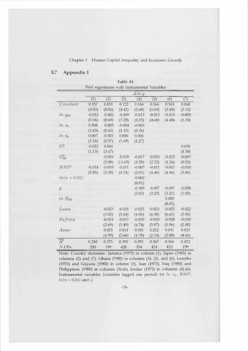
Chapter 3 Human Capital Inequality and Economic Growth
3.7 Appendix 1
Table AlPool regressions with Instrumental Variables
A ln y(1) (2) (3) (4) (5) (6) (7)
C o n s ta n t 0.157 0.031 0.122 0.166 0.166 0.165 0.068(4.03) (0.82) (4.42) (2.68) (5.63) (5.49) (2.12)
ln 2/60 -0.012 -0.002 -0.009 -0.013 -0.013 -0.013 -0.005(3.36) (0.69) (3.29) (3.33) (4.60) (4.48) (1.70)
ln s h 0.008(1.65)
-0.003(0.65)
-0.004(1.19)
-0.003(0.76)
ln Sk 0.007(1.16)
-0.003(0.57)
0.006(1.69)
0.006(1.27)
G v -0.023 0.044 0.038
Ggo
(1.15) (1.6 7) (1.50)-0.016 -0.018 -0.017 -0.023 -0.022 -0.007(1.08) (-1.63) (1.20) (2.22) (1.26) (0.55)
B M P -0.014 -0.010 -0.011 -0.007 -0.011 -0.011 -0.010(5.85) (3.50) (4.24) (2.01) (4.46) (4.46) (3.86)
Zn(n + 0.05) -0.000(0.01)
9 -0.109(2.83)
-0.097(3.23)
-0.097(3.21)
-0.058(1.82)
ln H qo 0.000(0.05)
L a a m -0.023 -0.021 -0.025 -0.025 -0.025 -0.022(3.82) (5.64) (4.56) (6.58) (6.61) (3.96)
S a f r i c a -0.024 -0.031 -0.029 -0.028 -0.028 -0.018(2.49) (5.49) (4.74) (5.97) (5.96) (2.00)
A s ia e 0.025 0.014 0.011 0.012 0.011 0.023(4.99) (2.66) (1.78) (2.14) (2.08) (4.66)
R ¿ 0.210 0.375 0.393 0.391 0.367 0.366 0.412N .O b s . 200 199 428 354 433 433 199
N ote- Country dummies: Jamaica (1975) in column (1), Japan (1965) in columns (2) and (7), Ghana (1980) in columns (3), (5), and (6), Lesotho (1970) and Guyana (1980) in column (3), Irán (1975), Iraq (1980) and Philippines (1980) in columns (3)-(6), Jordán (1975) in columns (4)-(6). Instrumental variables (variables lagged one period) for ln Sk, B M P , ln{n -I- 0.05) and g.
-74-
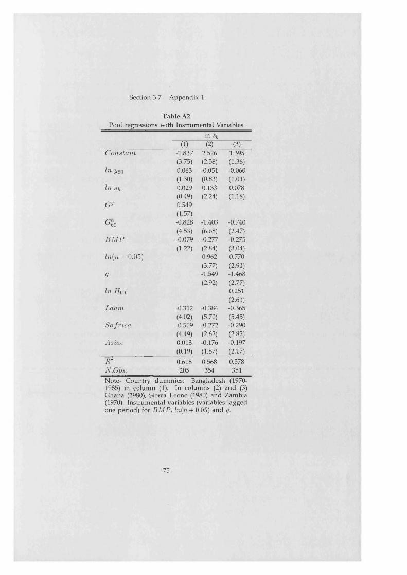
Section 3.7 Appendix 1
Table A2Pool regressions with Instrumental Variables
ln sk(1) (2) (3)
Constant -1.837 2.526 1.395(3.75) (2.58) (1.36)
ln yeo 0.063 -0.051 -0.060(1.30) (0.83) (1.01)
ln sh 0.029 0.133 0.078(0.49) (2.24) (1.18)
Gy 0.549(1.57)
^60 -0.828 -1.403 -0.740(4.53) (6.68) (2.47)
B M P -0.079 -0.277 -0.275(1.22) (2.84) (3.04)
ln(n + 0.05) 0.962 0.770(3.77) (2.91)
9 -1.549 -1.468(2.92) (2.77)
ln Hqo 0.251(2.61)
Laarn -0.312 -0.384 -0.365(4.02) (5.70) (5.45)
Safrica -0.509 -0.272 -0.290(4.49) (2.62) (2.82)
Asiae 0.013 -0.176 -0.197(0.19) (1.87) (2.17)
R ¿ 0.618 0.568 0.578N.Obs. 205 354 351
Note- Country dummies: Bangladesh (1970-1985) in column (1). In columns (2) and (3) Ghana (1980), Sierra Leone (1980) and Zambia (1970). Instrumental variables (variables lagged one period) for BMP, ln(n + 0.05) and g.
-75-

Chapter 3 Human Capital Inequality and Economic Growth
Table A3Cross-section regressions with Q3 as the human capital equality indicator
A ln y(1) (2) (3) (4) (5) (6) (7)
C o n s ta n t 0.197 0.102 0.127 0.141 0.112 0.116 0.090(6.69) (4.10) (7.03) (4.91) (7.42) (7.64) (5.15)
ln 2/60 -0.016 -0.011 -0.011 -0.013 -0.011 -0.011 -0.010(5.09) (4.30) (5.00) (6.05) (6.04) (6.35) (4.97)
ln Sh 0.014(3.60)
0.006(1.92)
0.005 (2.17)
0.006(2.29)
ln Sk 0.015(2.98)
0.005(1.18)
0.008(2.70)
0.005(1.64)
G y -0.032 0.045 0.041
Q lo
(2.09) (2.28) (2.26)0.031 0.023 0.025 0.038 0.028 0.042(3.03) (2.88) (2.82) (6.06) (3.10) (5.78)
B M P -0.007 -0.005 -0.005 -0.006 -0.005 -0.006 -0.004(1.78) (1.75) (2.57) (3.2 7) (3.07) (3.12) (1.52)
ln (n + 0.05) -0.001(0.13)
9 -0.056(2.67)
-0.071(3.61)
-0.065(3.35)
-0.067(3.17)
ln H qq 0.003(1.54)
L a a m -0.019 -0.014 -0.017 -0.020 -0.021 -0.023(4.45) (5.45) (5.02) (8.07) (8.15) (6.04)
S a f r i c a -0.023 -0.018 -0.018 -0.025 -0.025 -0.029(3.88) (4.55) (4.75) (7.73) (8.01) (6.37)
A s ia e 0.019 0.019 0.017 0.019 0.017 0.019(3.73) (4.28) (3.60) (3.51) (3.15) (3.03)
R 2 0.443 0.759 0.776 0.797 0.767 0.770 0.775N .O b s . 69 67 83 83 83 83 67
Note- Dum m ies for Botswana and Philippines in columns (2)-(7).
-76-

Section 3.7 Appendix 1
Table A4Cross-section regressions with Q3
Constant -1.851 1.102 1.101(2.70) (0.91) (0.91)
ln 2/eo 0.001 -0.062 -0.084(0.01) (0.78) (1.06)
ln s h 0.242 0.303 0.277(2.14) (3.00) (2.63)
G y 0.928(1.50)
Q l 0 0.746 0.952 0.488(2.15) (2.85) (1.24)
BMP -0.041 -0.272 -0.271(0.33) (1.51) (1.50)
ln (n 4- 0.05) 0.674 0.639(2.06) (2.05)
9 -1.794 -1.547(2.07) (1.91)
ln # 6 0 0.146(1.95)
Laam -0.286 -0.330 -0.350(2.10) (3.50) (3.79)
Safrica -0.192 -0.042 -0.099(0.73) (0.20) (0.48)
Asiae 0.017 -0.075 -0.143(0.14) (0.61) (1.20)
7 ? 0.638 0.688 0.701N.obs. 67 83 83Note- Dum m ies for Bangladesh in column (1) and for Mozambique in columns (2) and (3).
ln sk
(1) (2) (3)
-77-

Chapter 3 Human Capital Inequality and Economic Growth
Table A5Cross-section regressions for developing countries
A ln y(1) (2) (3) (4) (5) (6) (7)
Constant 0.201 0.093 0.124 0.144 0.115 0.111 0.090(5.75) (3.26) (4.88) (3.43) (5.59) (4.55) (3.22)
ln V60 -0.017 -0.010 -0.010 -0.011 -0.008 -0.008 -0.008(3.93) (2.55) (3.25) (3.73) (3.49) (3.58) (2.40)
ln Sfi 0.014(3.53)
0.004(1.24)
0.005(1.57)
0.005(1.69)
ln Sk 0.014(2.51)
0.003(0.70)
0.006(1.84)
0.004(0.99)
Gy -0.022 0.053 0.045
G heo
(0.78) (1.97) (1.69)-0.016 -0.018 -0.021 -0.031 -0.025 -0.026(1.29) (2.33) (2.62) (4.96) (1.76) (2.85)
B M P -0.005 0.002 -0.004 -0.006 -0.005 -0.005 0.001(0.87) (0.50) (1.55) (2.05) (2.68) (2.59) (0.24)
ln(n + 0 .05) 0.002(0.12)
9 -0.050(2.00)
-0.060(2.77)
-0.058(2.50)
-0.046(1.65)
ln Hqo 0.002(0.46)
Laam -0.014 -0.014 -0.018 -0.022 -0.022 -0.019(2.34) (4.02) (4.28) (6.36) (6.19) (3.66)
Safrica -0.020 -0.017 -0.018 -0.024 -0.024 -0.025(3.05) (4.40) (4.44) (7.27) (7.13) (4.55)
Asiae 0.026 0.021 0.017 0.018 0.017 0.023(4.14) (4.05) (2.96) (2.95) (2.80) (3.11)
i f 0.365 0.755 0.763 0.776 0.761 0.757 0.769N.Obs. 49 47 61 61 61 61 47
Note- Dum m ies for Botswana and Philippines in columns (2) to (7).
-78-

Section 3.8 Appendix 2
Table A6Cross-section regressions for developing countries
ln sk(1) (2) (3)
Constant -2.151 1.862 1.632(2.87) (1.16) (0.91)
ln 2/60 0.170 -0.019 -0.022(1.69) (0.16) (0.19)
ln s h 0.131 0.280 0.275(1.18) (2.37) (2.16)
G y 0.419(0.58)-1.003 -1.026 -0.832(3.14) (3.77) (1.74)
BMP -0.150 -0.293 -0.291(0.98) (1.69) (1.66)
ln (n + 0.05) 0.798 0.767(2.11) (2.01)
9 -1.487 -1.412(1.70) (1.55)
Iu H qo 0.057(0.48)
Laam -0.459 -0.429 -0.424(2.27) (3.3 7) (3.31)
Safrica -0.201 -0.084 -0.091(0.72) (0.42) (0.44)
Asiae -0.080 -0.146 -0.161(0.46) (0.98) (1.09)
R 1 0.598 0.618 0.612N.obs. 47 61 61
Note- Dummies for Senegal and Bangladesh in col- umn (1) and for Mozambique in columns (2) and(3).
-79-

Chapter 3 Human Capital Inequality and Economic Growth
3.8 Appendix 2
Human capital Gini coefficient and distribution of education by quintiles for 108 countriesObs. Cov G h St. Dv Qi q 2 Qs Q4 H
M . East & N.Africa 100 60-00 0.583 0.180 0.009 0.051 0.165 0.407 3.931DZA 9 60-00 0.657 0.140 0.000 0.012 0.098 0.327 2.908EGY 6 75-00 0.621 0.130 0.000 0.006 0.108 0.402 3.703TUN 9 60-00 0.665 0.157 0.000 0.011 0.101 0.331 2.783BHR 9 60-00 0.591 0.169 0.000 0.034 0.144 0.420 3.656IRN 9 60-00 0.683 0.149 0.000 0.006 0.076 0.299 2.905IRQ 9 60-00 0.725 0.143 0.000 0.000 0.059 0.257 2.273ISR 9 60-00 0.214 0.033 0.070 0.249 0.466 0.710 8.718JOR 9 60-00 0.533 0.114 0.000 0.034 0.178 0.503 4.549KWT 9 60-00 0.566 0.070 0.000 0.002 0.163 0.478 4.451SYR 9 60-00 0.548 0.129 0.000 0.049 0.167 0.478 3.621YEM 4 75-90 0.913 0.064 0.000 0.000 0.000 0.015 0.688CYP 9 60-00 0.277 0.060 0.041 0.207 0.416 0.667 6.912S. Saharian Africa 237 60-00 0.637 0.164 0.001 0.024 0.119 0.365 2.430BEN 7 70-00 0.812 0.083 0.000 0.000 0.000 0.134 1.443BWA 9 60-00 0.521 0.132 0.000 0.046 0.177 0.527 3.526CMR 9 60-00 0.620 0.095 0.000 0.001 0.116 0.411 2.522CAF 9 60-00 0.793 0.101 0.000 0.000 0.007 0.167 1.461COG 4 85-00 0.481 0.014 0.000 0.020 0.219 0.588 5.099GMB 6 75-00 0.826 0.080 0.000 0.000 0.000 0.114 1.465GHA 9 60-00 0.654 0.096 0.000 0.000 0.069 0.362 2.992GNB 5 80-00 0.823 0.065 0.000 0.000 0.000 0.120 0.604KEN 9 60-00 0.551 0.132 0.000 0.034 0.174 0.482 2.913LSO 9 60-00 0.354 0.012 0.000 0.117 0.388 0.659 3.771LBR 9 60-00 0.782 0.089 0.000 0.000 0.005 0.170 1.655MWI 9 60-00 0.556 0.061 0.000 0.000 0.134 0.532 2.500MLI 9 60-00 0.908 0.026 0.000 0.000 0.000 0.000 0.524MRT 1 90 0.625 0.000 0.000 0.000 0.077 0.445 2.424MUS 9 60-00 0.343 0.067 0.022 0.155 0.358 0.638 4.785MOZ 9 60-00 0.768 0.068 0.000 0.000 0.000 0.189 0.766NER 9 60-00 0.901 0.039 0.000 0.000 0.000 0.000 0.586RWA 7 70-00 0.652 0.105 0.000 0.000 0.065 0.384 1.886SEN 9 60-00 0.649 0.042 0.000 0.000 0.060 0.416 2.093SLE 9 60-00 0.823 0.078 0.000 0.000 0.000 0.123 1.562ZAF 9 60-00 0.408 0.089 0.000 0.086 0.310 0.614 4.892
-80-

Section 3.8 Appendix 2
Human capital Gini coefficient and distribution of education by quintiles for 108 countriesObs. Cov G h St. Dv. Qi q2 Q3 q4 H
SDN 9 60-00 0.793 0.077 0.000 0.000 0.000 0.162 1.170SWZ 9 60-00 0.473 0.144 0.000 0.066 0.231 0.563 4.091TZA 9 60-00 0.462 0.051 0.000 0.015 0.277 0.607 2.859TGO 9 60-00 0.734 0.141 0.000 0.000 0.062 0.232 1.901UGA 9 60-00 0.620 0.120 0.000 0.010 0.099 0.412 2.111ZAR 9 60-00 0.657 0.091 0.000 0.000 0.066 0.349 1.970ZMB 9 60-00 0.443 0.108 0.004 0.076 0.274 0.588 3.794ZWE 9 60-00 0.435 0.096 0.016 0.067 0.282 0.596 3.106L. America & Caribbeati 207 60-00 0.367 0.136 0.042 0.156 0.339 0.593 4.784BRB 9 60-00 0.196 0.042 0.117 0.266 0.455 0.697 7.730CRI 9 60-00 0.281 0.015 0.059 0.236 0.413 0.634 5.025DOM 9 60-00 0.450 0.033 0.000 0.056 0.294 0.571 3.780SLV 9 60-00 0.466 0.094 0.000 0.068 0.273 0.558 3.408GTM 9 60-00 0.604 0.080 0.000 0.001 0.122 0.441 2.442HTI 9 60-00 0.736 0.127 0.000 0.000 0.052 0.236 1.929HND 9 60-00 0.459 0.106 0.003 0.081 0.265 0.554 3.244JAM 9 60-00 0.245 0.029 0.100 0.255 0.416 0.652 3.996MEX 9 60-00 0.372 0.076 0.021 0.130 0.350 0.617 4.906NIC 9 60-00 0.533 0.063 0.000 0.024 0.214 0.498 3.291PAN 9 60-00 0.299 0.057 0.038 0.202 0.399 0.646 6.332TTO 9 60-00 0.235 0.023 0.101 0.253 0.424 0.665 6.318ARG 9 60-00 0.202 0.010 0.111 0.278 0.458 0.682 6.972BOL 9 60-00 0.454 0.037 0.000 0.057 0.272 0.580 5.004BRA 9 60-00 0.426 0.099 0.008 0.121 0.322 0.540 3.561CHL 9 60-00 0.245 0.034 0.084 0.246 0.420 0.675 6.266COL 9 60-00 0.396 0.025 0.002 0.147 0.328 0.581 4.165ECU 9 60-00 0.369 0.033 0.012 0.151 0.348 0.611 5.008GUY 9 60-00 0.202 0.011 0.102 0.279 0.459 0.691 5.211PRY 9 60-00 0.268 0.019 0.063 0.242 0.424 0.644 4.939PER 9 60-00 0.365 0.074 0.020 0.138 0.347 0.616 5.449URY 9 60-00 0.255 0.021 0.091 0.242 0.413 0.658 6.372VEN 9 60-00 0.386 0.102 0.024 0.118 0.330 0.601 4.690East Asia & Pacific 90 60-00 0.377 0.137 0.028 0.143 0.331 0.599 5.558HKG 9 60-00 0.332 0.071 0.023 0.156 0.371 0.655 7.592IDN 9 60-00 0.503 0.114 0.000 0.045 0.224 0.534 3.382KOR 9 60-00 0.298 0.126 0.040 0.183 0.405 0.663 7.674MYS 9 60-00 0.414 0.086 0.006 0.110 0.305 0.586 4.943
-81-

Chapter 3 Human Capital Inequality and Economic Growth
Human capital Gini coefficient and distribution of education by quintiles for 108 countriesObs. Cov Gh St. Dv. Qi q 2 Qs q4 H
PHL 9 60-00 0.263 0.066 0.067 0.226 0.422 0.657 6.213SGP 9 60-00 0.413 0.070 0.005 0.091 0.283 0.622 5.643OAN 9 60-00 0.329 0.086 0.029 0.157 0.377 0.647 6.728THA 9 60-00 0.313 0.046 0.028 0.190 0.410 0.637 4.888FJI 9 60-00 0.199 0.041 0.078 0.272 0.474 0.710 6.691PNG 9 60-00 0.709 0.102 0.000 0.000 0.038 0.277 1.821South Asia 63 60-00 0.697 0.167 0.003 0.024 0.080 0.267 2.400AFG 9 60-00 0.862 0.025 0.000 0.000 0.000 0.009 1.329BGD 9 60-00 0.749 0.106 0.000 0.000 0.027 0.209 1.637BUR 9 60-00 0.651 0.111 0.000 0.007 0.099 0.345 1.887IND 9 60-00 0.656 0.069 0.000 0.000 0.047 0.386 3.242NPL 9 60-00 0.866 0.110 0.000 0.000 0.004 0.080 0.999PAK 9 60-00 0.757 0.105 0.000 0.000 0.029 0.191 2.336LKA 9 60-00 0.339 0.055 0.023 0.163 0.356 0.649 5.367Advanced Countries 207 60-00 0.208 0.093 0.103 0.253 0.455 0.696 7.940CAN 9 60-00 0.142 0.023 0.111 0.293 0.510 0.745 10.205USA 9 60-00 0.131 0.041 0.133 0.303 0.513 0.742 10.658JPN 9 60-00 0.169 0.013 0.122 0.270 0.485 0.720 8.399AUT 9 60-00 0.189 0.011 0.087 0.243 0.489 0.735 7.605BEL 9 60-00 0.180 0.019 0.125 0.274 0.464 0.710 8.526DNK 9 60-00 0.169 0.008 0.114 0.266 0.494 0.722 9.134FIN 9 60-00 0.165 0.030 0.138 0.295 0.480 0.397 7.543FRA 9 60-00 0.217 0.024 0.127 0.260 0.422 0.674 6.508DEU 9 60-00 0.200 0.031 0.080 0.231 0.478 0.729 8.977GRC 9 60-00 0.264 0.028 0.064 0.232 0.419 0.660 6.724ISL 9 60-00 0.182 0.018 0.134 0.278 0.460 0.695 7.335IRL 9 60-00 0.185 0.013 0.117 0.274 0.464 0.710 7.694ITA 9 60-00 0.280 0.034 0.067 0.216 0.400 0.656 5.935NLD 9 60-00 0.159 0.022 0.120 0.284 0.502 0.721 7.839ÑOR 9 60-00 0.140 0.040 0.139 0.306 0.501 0.725 8.795PRT 9 60-00 0.437 0.068 0.017 0.102 0.294 0.549 3.727ESP 9 60-00 0.258 0.024 0.075 0.239 0.422 0.664 5.477SWE 9 60-00 0.185 0.030 0.110 0.256 0.474 0.717 9.366CHE 9 60-00 0.205 0.028 0.098 0.256 0.462 0.705 9.250TUR 9 60-00 0.512 0.090 0.000 0.043 0.213 0.516 3.472GBR 9 60-00 0.173 0.023 0.125 0.277 0.474 0.717 8.329AUS 9 60-00 0.129 0.005 0.120 0.311 0.521 0.738 10.249
-82-
Section 3.8 Appendix 2
Human capital Gini coefficient and distribution of education by quintiles for 108 countriesObs. Cov G h St. Dv. Qi q 2 q3 q4 H
NZL 9 60-00 0.111 0.019 0.136 0.317 0.527 0.755 10.876Transitional Economies 31 60-00 0.223 0.106 0.082 0.246 0.447 0.697 7.045CHN 6 75-00 0.381 0.069 0.003 0.110 0.323 0.644 5.401H U N 9 60-00 0.125 0.021 0.153 0.325 0.509 0.724 8.305POL 9 60-00 0.126 0.018 0.143 0.318 0.514 0.736 8.517YUG 7 60-90 0.259 0.019 0.027 0.230 0.441 0.684 5.959
TOTAL 935 60-00 0.438 0.239 0.039 0.127 0.278 0.523 4.809
-83-


Chapter 4 Inequality, Life Expectancy and Development
4.1 IntroductionSince the last decade there has appeared an increasing body of literature that an- alyzes the influence that inequahty in the distribution of income or wealth may exert on economic growth and income diíferentials across countries. The complex- ity of the relationship between inequahty and growth has led theoretical models to look at this problem in different ways. Broadly, the literature has focused on two mechanisms through which inequahty may influence growth.1
This chapter explores an altemative channel through which inequahty in the distribution of hum an capital may influence the process of hum an capital accumu- lation. This new mechanism is based on the relationship between hum an capital distribution, Life expectancy and the accumulation of human capital.
Some models that have analyzed the relationship between demography and development have noticed the important role played by life expectancy in deter- mining the optimal education decisions of individuáis. For example, Erich and Luí (1991) focus on a theoretical model that links longevity, fertihty and economic growth to explain “demographic transition” . In their overlapping generation model, a sufficient exogenous increase in longevity promotes economic growth as well as reduces fertihty rates. In a similar model, Blackburn and Cipriani (2002) en- dogenize life expectancy. As a result, their model generates múltiple developm ent regimes depending on initial conditions. Endogenizing life expectancy al- lows Blackburn and Cipriani (2002) to explain jointly the main changes that take place during the demographic transition of economies, such as greater life ex-
typectancy, higher levels of education, lower fertihty and later timing of births.
1 Benabou (19%) or Aghion, Caroli and García-Peñalosa (1999) survey this literature.2 De la Croix and Licandro (1999) and Kalmeli-Ozcan, Ryder and Weil (2000), among others, have developed continuous time overlapping generations models in which optimal schooling investment decisions depend positively on life expectancy. In addition, the im- portance of life expectancy in models with endogenous fertihty rates and hum an capital investment decisions is also revealed in the recent papers of Kalemli-Ozcan (2001), Soares
-84-
Section 4.1 Introduction
The main purpose of this chapter is to include endogenous life expectancy in a model populated by heterogeneous agents. In our model individuáis live for two periods and differ in their second period survival probability. In particular, we consider that life expectancy is conditioned by the hum an capital of the fami- lies which individuáis are bom into. Given their expected survival probabilities, individuáis choose the optimal time devoted to becoming educated in order to maximize their intertemporal utility.
The survival probability function is calibrated according to the data and, as a result, the model shows múltiple steady States.4 In particular, the time individuáis devote to hum an capital accumulation converges towards two steady States: poor individuáis converge to a low steady state and rich individual converge to a high steady state. Consequently, the initial distribution of wealth determines the long- term average hum an capital and the average income in the economy. The fewer the num ber of individuáis with education lower than a threshold level, the greater the average hum an capital and average income in the economy.
Although the policy implications we obtain are quite similar to those of Ga- lor and Zeira (1993), the underlying assumptions of the models are different. In their model the assumptions of imperfect credit markets and indivisibilities in human capital investment are crucial for the results. In our model, the results are mainly due to the assumption of differences in the survival probabilities among individuáis. Henee, in Galor and Zeira (1993) model, poor individuáis would in- vest more hum an capital if capital markets were perfect. In our model, even with perfect capital markets, poor individuáis invest a low amount of hum an capital since their low life expectancy increases their opportunity cost of becoming educated.
The structure of this chapter is as follows. Section 4.2 displays the basic structure of the model. Section 4.3 calibrates the model and analyses the rela-
(2001) and Tamura (2002).3 Recently, Case, Lubostky and Paxon (2001) give evidence of a positive relationship between household income and children health.4 Other models with heterogeneous agents that generate múltiple steady states, without assuming non-convexities in the production process, are the recent papers of Moav (2001) or Eicher and García-Peñalosa (2001). In Moav (2001), parents face a trade-off between child quality and child quantity. The endogenous fertility choice in this model results in múltiple steady states. In Eicher and García-Peñalosa (2001), the key assumption for the existence of múltiple steady states is the interdependence of supply and dem and for skilled workers under skilled-biased technological change. Azariadis (2001) offers an excellent survey on the literature about poverty traps.
-85-
Chapter 4 Inequality, Life Expectancy and Development
tion between inequality and growth. Finally, Section 4.4 presents the conclusions reached.
4.2 The modelIn this section we present a very simple model to analyze the relationship between inequahty, Ufe expectancy and growth. For this purpose we consider an overlapping generation model in which individuáis can Uve at most for two periods. The probability of living during the whole first period is one, whereas the probability of living until the end of the second period is TTt+i- At the end of the first period each individual gives birth to another such that all individuáis have a descendent. In every period the economy produces a single good that is used for consumption.
4.2.1 Life expectancyThe economy is populated by individuáis that differ in their family wealth but that are identical in their preferences and innate abilities. We assume that an individual^ life expectancy will depend on the economic status of the family which the individual is bom into.
The empirical evidence shows a negative association between socioeconomic status and mortality. Marmot et al. (1991) found in the Whitehall II study a pos- itive association between the grade of employment of British civil servants and their health status, a result already obtained in the first Whitehall study initiated in 1967. Some papers have also suggested that this relation is not linear. Smith (1999) analyses the relation between individuáis' health and their income or wealth us- ing the Health and Retirement Survey (HRS) for 12,000 American individuáis. He estimates an order probit model with self reported health status as the dependent variable.5 The results show that the relationship between self reported health and income or wealth is non-linear, and that the positive and statistically significant effect of income and wealth on self reported health status decreases as socioeconomic status increases.
On this matter, Case, Lubotsky and Paxon (2001) suggest that the gradient, that is, the positive association between health and socioeconomic status, has its origins in childhood. They provide evidence of a positive relationship between household income and child health. Currie and Hyson (1999) find that being bom
5 Smith, Taylor and Sloan (2001), using the HRS, find that subjective perceptions of mortality are good predictors of observed mortality.
-86-

Section 4.2 The model
in a low socioeconomic status family increases the probability of reporting poor health at age 23 and 33. Regarding medical studies, many of them have found an association between the environment in early life and the development of dis- eases in later life. Ravelli et al. (1998) investígate glucose tolerance in people bom around the time of famine in the Netherlands during 1944-1945. They found that prenatal exposure to famine, especially during late gestation, was linked to de- creased glucose tolerance in adults producing a higher risk of diabetes. Barker (1997) focuses on the “fetal origins” hypothesis which states that hum an fetuses change their physiology and metabolisms in order to adapt to a limited supply of nutrients. These programmed changes may be the origins of a number of diseases in later life such as coronary heart disease, strokes, diabetes and hypertension. W adsworth and Kuh (1997) state that poor conditions at home during early life predict high systolic blood pressure at age 43 and reduced peak expiratory flow rate at age 36.
The foregoing results suggest that it is realistic to assume that individuáis bom in rich families will have higher life expectancy than those born in poor fam- ilies, who are more likely to be affected by undemourishment during early stages of life and an unhealthier environment during childhood, for instance, lower stan- dards of hygiene at home, an unhealthier diet or less use of preventive and cu-rative medical Services. Moreover, we consider that the positive effect that familyincome may exert on an individual life expectancy decreases as income increases and vanishes at high income levels. In particular, as hum an capital is one of the main determinants of income and wealth, we assume that parents' hum an capital will determine the survival probability of their children. Thus, we consider a positive but decreasing effect of parents' hum an capital on the life expectancy of their descendants. The probability of an individual i born in period t surviving to different periods (t + n) is as follows:
{ 1 for n = 0 \t f í t+ itá T 1) f o rn = l > (4.1)
0 for n > 2 J
where h is the hum an capital of the parent. In the next section we use a spe- cific equation for the survival probability according to the empirical evidence of the relationship between life expectancy and schooling years. Given that the evidence is only available for schooling years, throughout the paper we make the survival probability depend on parents' schooling years instead of a broad con-
-87-

Chapter 4 Inequality, Life Expectancy and Development
cept of hum an capital.
4.2.2 TechnologyIn the first period of life individuáis are endowed with one unit of time. They allocate L\ units towards producing final goods with the following technology:
Hit = AL\t (4.2)
where A is a function of the level of technology and other production inputs and 0 < L\t < 1. For simphcity, we consider that A is constant.
Individuáis allocate the remaining units of their time (1 — L\) towards ac- quiring formal education for the second period according to the function:
h\t+i = ^(1 — L\t) (4.3)
where 9 is the number of years of the first period and h\t+1 the schooling years that individual i accumulates when young.
In the second period of life, individuáis allocate all their time endowment to the production sector such that,
y¡t+ 1 = AL\t+leah"+> (4.4)
where L \t+1 = 1. Thus, the higher the hum an capital stock accumulated during the first period the higher the income produced in the second period. The specifi- cation of the production function in the second period relies on the work of Mincer (1974), since it relates the log of income to schooling years
ln y¡t+1 = ln A + a h \t+l (4.5)
Therefore, the coefficient a can be interpreted as the return of education.
4.2.3 PreferencesThe preferences of an individual born in t are represented by a log-linear utility function of the form:
u\ = l n 4 + lA t+ Á htü l ) ln 4 + i (4*6)
The expected lifetime utihty is defined over consumption when yotrng ( 4 ) and consumption when oíd ( 4 +1), where the second period utility is discounted for the endogenous survival probability and for the rate of time prefer-ence p, where 7 = 1 /(1 + p).
-88-

Section 4.2 The model
During the first period, agents can finance their consumption with two types of income. The first one is given by the production of goods (yjt) which, as equa- tion (4.2) states, is a function of the time devoted to production. During the time they invest in education, we assume they have access to a minimum income per schooling year. Thus, the level of consumption in t is given by
4 t = v \ t + f3A(l-L\t) (4.7)
where (3 is a parameter, such that 0 < P < 1, which determines the revenue that covers the consumption whereas this agent is attending to school, net of all education cost. For simplicity, we assume that (3 is exogenous and that this revenue increases with A, that is, consumption during education years is higher in economies with higher A. In most economies, the revenue financing consumption whereas attending to school, which is thus proportional to (1 — L\^), is jointly fi- nanced by parents and public policies such as grants. Theoretical models usually incorpórate bequests as a basic resource for financing education years. However, as long as bequests are a function of parents' incomes, this constitutes an impor- tant channel through which the human capital of parents affects the human capital of theirs descendants. Since we are interested in analyzing these effects exclusively through the endogenous life expectancy, it is convenient to assume that individuáis can substitute intertemporally some income, proportional to the time they invest in education but independent from the schooling years of their parents. Thus, if (3 = 0 the intertemporal substitution of income for education is not allowed and welfare during the first period is entirely determined by y\t .
In the second period, total income is used to finance prívate consumption and to pay back the income consumed during the education years of the first period:
cít+1 = Vit+i t “ L\t) (4.8)'Xit+ÁKt )
For simplicity, we are assuming that the intertemporal substitution of income, which is only allowed for education, occurs at no cost. However, equation (4.8) takes into account the fact that individuáis may not live the whole second period. Dividing the (3A{1 — L\̂ ) by the endogenous life expectancy agents pay back this income independently of the number of years they live in the second period.
The model makes clear that agents with no probability of living during the second period, because the human capital of their parents is so low, will not al-
-89-

Chapter 4 Inequality, Life Expectancy and Development
lócate any fraction of their time to acquiring education. At the other extreme, if = then (1 — L lit) will reach its máximum valué. In other word, the
time individuáis devote to education will be a function of the schooling years of their parents, but exclusively through the endogenous life expectancy since inter- generational transfers are nonexistent.
4.2.4 Optimal education yearsThe optimal behavior of agents is to choose the amount of hum an capital that maximizes their intertemporal utility function. Thus, individual i chooses the time devoted to schooling, L \t , that maximizes (4.6) subject to the production functions (4.2) and (4.4), the accumulation of hum an capital (4.3), the budget restrictions (4.7) and (4.8), and the non-negativity and inequality restrictions (0 < L \t < l ) .6
For 0 < L \t < 1, the first order condition for this problem gives place to a non-linear function of L \t in terms of h ^ 1 and the different parameters of the model:
(1 - 0) íe x p {aé>(l - L\t)} - —— Jjprji1 ~ ¿ í t ) J = 7*4+1 (Mi- 1 )
( a 0 e x p { a 0 ( l - L ‘t) } - / 3 ) + (4-9)\ * it+ ú nu > )
As we show below, the time individuáis devote to accumulating hum an capital increases, at a decreasing rate, with their second period survival probability. Since the income in the second period depends on the time agents devote to accumulating hum an capital, the longer they expect to live the greater their hum an capital investment.
4.3 Inequality and GrowthIn this section we analyze the relationship between inequality in the distribution of education, life expectancy, hum an capital accumulation and income growth. Firstly, we calibrate the model. Then, we display the numerical results of the evo- lution of hum an capital over time. Finally, we explore how inequality may affect life expectancy, hum an capital and growth.
6 See Appendix 1.
-90-

Section 4.3 Inequality and Growth
4.3.1 CalibrationTo analyze the influence that inequahty in the distribution of hum an capital ex- erts on the process of development, following Blackburn and Cipriani (2002), we assume a specific function for the second period survival probability:
t j l + i r m ( h t r 1 )^7r*t+i ( h it ) = T T — 7üt- i \ é with w and 0 > 0 (4.10)
i + r
We choose this function due to its good properties. Thus, it is an increasing function of hum an capital
> 0 (4.11)
and it is bounded by 7r and 7T since
* i+ i(°)= :Z L (4.12)
and
lim 7l i+ i^ i t -1 ) = ñ < 1 (4.13)n—► oo
Apart from its theoretical properties, at the empirical level this function captures very weU the relationship between life expectancy and hum an capital across countries, for appropriate valúes of its parameters. Since micro data relating par- ents' education with offspring life expectancy for a broad number of countries are not available, we rely on aggregate data. Figure 4.1 shows the dispersión between life expectancy at birth in 1985, taken from the World Bank, and the average schooling years for the population 25 years oíd and over in 1960, from Barro andLee (2001). The different reference years for these two variables try to capture ourassumption that the survival probability in t + 1 of the generation bom in t is a
TJfunction of the hum an capital of generation bom in t — 1. This figure shows a
Qclear concave relationship between the stock of hum an capital and life expectancy.
7 Life expectancy at birth is defined as the niunber of years a newbom infant would live if prevailing pattems of mortality at the time of its birth were to stay the same throughout its life. Since Science is in continuous evolution, the prevailing pattems of mortality in 1960 changed in 1970 and so on. Therefore, in some way, life expectancy in 1985 is collecting the pattems of mortality in 1985 of people bom before this year.8 The concave shape holds with the different available years in the sample. In addition, infant mortality relates negatively at a decreasing rate with the stock of human capital. The relationship between infant mortality and the stock of human capital may proxy the
-91-
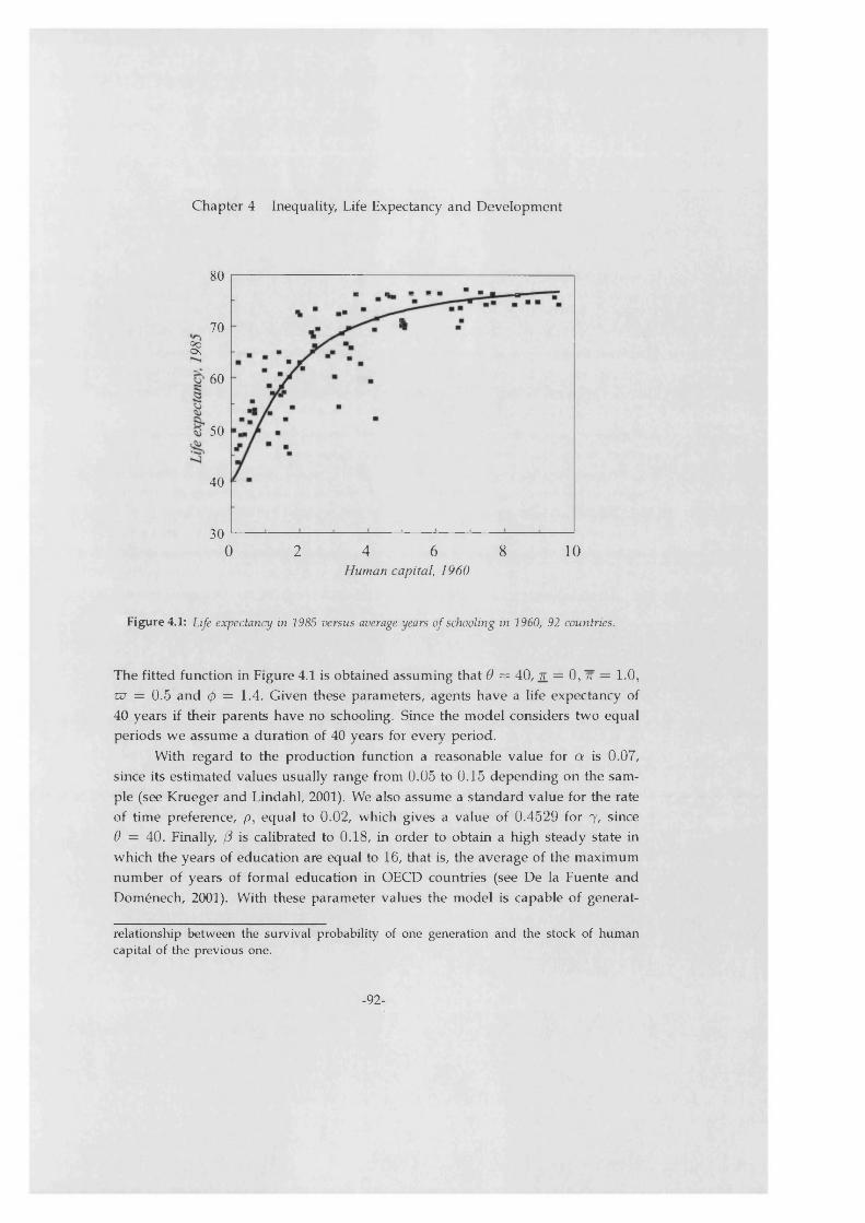
Chapter 4 Inequality, Life Expectancy and Development
80
7 0°oOs
6 0
5 0
40
3 00 2 4 6 8 10
Human capital, 1960
Figure 4.1: Life expectancy in 1985 versus average years of schooling in 1960, 92 countries.
The fitted function in Figure 4.1 is obtained assuming that 0 = 40, 7r = 0 , 7T = 1.0, w = 0.5 and 0 = 1.4. Given these parameters, agents have a life expectancy of 40 years if their parents have no schooling. Since the m odel considers two equal periods w e assum e a duration of 40 years for every period.
With regard to the production function a reasonable valué for a is 0.07, since its estimated valúes usually range from 0.05 to 0.15 depending on the sam- ple (see Krueger and Lindahl, 2001). We also assume a standard valué for the rate of time preference, p, equal to 0.02, which gives a valué of 0 .4529 for 7 , since 6 = 40. Finally, ¡3 is calibrated to 0.18, in order to obtain a high steady state in which the years of education are equal to 16, that is, the average of the máximum number of years of formal education in OECD countries (see De la Fuente and Doménech, 2001). With these parameter valúes the m odel is capable of generat-
relationship between the survival probability of one generation and the stock of human capital of the previous one.
-92-

Section 4.3 Inequality and Growth
ing múltiple steady states. Nevertheless, we also explore how the changes in these parameters affect the properties of the model.
4.3.2 The evolution of human capitalEquation (4.9) summarizes the dynamics of the model across generations and it is represented in Figure 4.2, given the valúes of the parameters discussed above.9 As we can observe, the number of years devoted to the education of the offspring increases with the hum an capital of the parents, except for low valúes of h ^ 1 where hlt+1 is equal to zero. The economy exhibits three different steady states: there are two low steady states with valúes of zero and around 3.5 years of schooling, and a high steady state of 16 years of schooling. However, since h*¿~1 = h\t+l = 3.5 is not a stable steady state, the dynamics of the model involve that individuáis with parents having less than 3.5 years of education (that is, primary education not completed) will converge to the lowest steady state with no schooling.
In Figure 4.3 we present the sensitivity of hum an capital steady states to changes in the different parameters of our model. As expected, an increase in the revenues to finance consumption in the first period (i.e., an increase in ¡3) results in an upward shift of the function relating human capital of the two generations. It can be shown that, given the calibrated valúes of the other parameters, when (3 = 0 the model exhibits only one steady state in which = h\t+l = 0, which can be interpreted as a credit market restriction for the whole economy, that is, this case entails the unreal situation in which there are not credit markets in the economy. Nevertheless, we can assume, as analyzed by Galor and Zeira (1993), that there are some individuáis in the economy who are restricted. Lets assume that those individuáis born in poor families with no education have not any collateral and, henee, are restricted in the credit market. In our model, however, this kind of restrictions in the credit market do not change the results since poor individuáis, even being allowed to get a credit, do not invest in education because their low life expectancy increases their opportunity cost of becoming educted. There- fore, the model prediets múltiple steady states with perfect credit markets as well as with the existence of credit restricted individuáis. An increase in the retums of education or in the life horizon (a and 0, respectively) and a reduction of the rate of time preference (p) also produces an upward shift of the function since the investment in education is more profitable. Finally, an increase of the survival probability for any given level of h ^ 1, through higher 0 or u , creates more education
9 See Apendix 2.
-93-

Chapter 4 Inequality, Life Expectancy and Development
incentives.Figure 4.2 makes clear that individuáis who are bom into poor families
with low levels of education { h \ j l ~ 0) will have a low survival probability (7r¿+1(h*¿-1) ~ 0) and, therefore, have no incentives to accumulate hum an capital (ih\t+l ~ 0), devoting all their time to working in the production sector {L\ = 1), with a low productivity. This low steady state is found in some Latín American, African or South Asian countries, in which many children born in poor families, with no education, live for a short period of life, have no access to education and work as unskilled workers from childhood, affecting a large share of the world populatíon. Using Barro and Lee (2001) data for 2000, at least 20 per cent of the population 15 years oíd and over was illiterate in 50 of the 108 countries in the sample. In 25 of these countries, at least 40 per cent of the population was illiterate. The share of the population with no education is 80 percent in Mali and Niger, where the life expectancy at birth is 43 and 46 years, respectively.
The dynamics of the model predict that govemments could bring these families out of the no schooling poverty trap if they guarantee access to a mínimum level of education for some generations and increase life expectancy.
4.3.3 Human capital distribution, life expectancy and growthIn accordance with the previous results, in this model the initial distribution of wealth will determine the long-run average hum an capital and average income in the economy. Given the simplifying assumptions we have made the model does not exhibit endogenous growth in the steady states, but it is useful to explain one source of the per capita income differentials across countries. Thus, the fewer the num ber of individuáis with education lower than the threshold level, the greater the average hum an capital and average income in the economy.
Under the assumption of imperfect credit markets and indivisibüitíes in human capital investment, Galor and Zeira (1993) obtain similar results. In their model the initial distribution of wealth determines the share of the population with no education that works as unskilled workers. Likewise, their model also shows the possibility of two steady states, a low steady state with unskilled workers and a high one with skilled workers. However, the underlying assumptions of their models are quite different to ours. In Galor and Zeiras model, the assumption of imperfect credit markets causes that the distribution of wealth influences economic activity in the short term, and indivisibilities in hum an capital investm ent are crucial in order to preserve these results in the long run. In contrast,
-94-
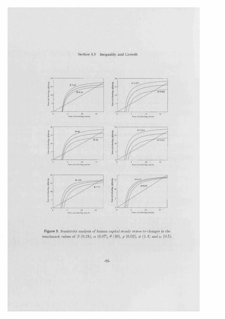
Year
s of
scho
olin
g, o
ffspr
ing.
Ye
ars o
f sc
hool
ing,
offs
prin
g.
Year
s of
scho
olin
g, o
ffspr
ing.
Section 4.3 Inequality and Growth
20
0 = 0-2015
10
5
00 5 10 15Years o f schooling, parenl.
20
a= 0.075
15
10
5
00 5 10 15Years o f schooling, paren!.
20
15
10
5
00 5 10 15Years o f schooling, parenl.
20p=0.018
15
p=0.022
10
5
00 5 10 15Years o f schooling, paren!.
20
15
«►=1.15
10
5
00 5 10 15Years o f schooling, paren!.
(0=0.6515
10
5
00 5 10 15Years o f schooling. parenl.
Figure 3: Sensitivity analysis of human capital steady states to changes in the benchmark valúes of ¡3 (0.18), a (0.07), 9 (40), p (0.02), (¡) (1.4) and u (0.5).
-95-

Chapter 4 Inequality, Life Expectancy and Development
bo•S"C
Io•«0<>a
e1
15
10
5
00 105 15
Years o f schooling, parent.
Figure 4.2: Human capital dynamics.
the results of our m odel are mainly due to the assumption that differences in the survival probabilitíes am ong individuáis are a function of their parents' human capital.
The existence of múltiple steady States depending on initial conditions makes clear that the initial distribution of education matters a great deal for the evolu- tion of the average human capital in the economy. On this matter, it can be easily show n that, given two countries with the same average human capital stock in one period, the country with the greater inequality w ill exhibit lower average survival probability and, therefore, a lower stock of human capital in the follow ing period. Assum ing that the econom y is populated by a fraction A = 0.2 of rich individuáis, denoted by r, and a fraction (1 — A) of poor individuáis, denoted by p, in Figure 4.4 w e have represented the average survival probability, for two econom ies with averages of 5 and 6 schooling years, as a function of the equality index (e), that is
-96-

Section 4.3 Inequality and Growth
h=6
h=5
0 0.2 0.4 0.6 0.8Equality índex
Figure 4.4: Average survival probability and human capital equality index (^pt+i/^rt+i)-
constructed as the ratio between the human capital of poor and rich individuáis
<* = #i<414>r , t
As w e can observe, for an equality index higher than 0.4 the average survival probability increases very slowly, but when the index is below 0.4, this probability decreases rapidly as the distribution of human capital becomes more unequal.
The empirical evidence supports this implication of the model. Using the calibrated function for the survival probability, w e have estimated the following equation for a sam ple of 92 countries:
LEi, 1985 = ^min "b (^m ax ^ m in ) ^ ,1985(^1,1960) "T f^Gh^1960 (4-15)
where i refers to the different countries in the sample, the dependent variable is the life expectancy in 1985 (from the World Bank), h is measured as the average years of schooling in 1960 (from Barro and Lee, 2001) and G h is the Gini coefficient of human capital in 1960 taken from Castelló and Doménech (2002), in deviations
-97-

Chapter 4 Inequality, Life Expectancy and Development
Table 4.1Life expectancy and inequality
(1) (2)$min 64.38 52.08
(106.5) (21.2)^max 64.38* 73.18
(43.9)-29.58 -10.69(13.5) (2.72)
d i — -13.54(8.60)
d 2 - 11.76
R 2(6.11)
0.666 0.867Obs. 92 92
t-ratios in parenthesis. * restricted parameter.
from the sample average. The estimated valué of 0 m in is the life expectancy of a country where average schooling years are zero and the Gini coefficient is equal to the sample average. The equation also includes two dummy variables di (for Congo, Cote d'Ivoire, Ethiopia, Kenya, Mauritius, and Zambia) and d2 ( for Jordán, Mauritania, Nicaragua and the United States) which control for outliers, since their residuals exceed in more than three times the estimated standard error of the residuals. As w e can observe in Table 4.1, equation (4.15) explains a large variance (86.7 per cent) of life expectancy across countries with just two variables dated in 1960. In column (1) w e regress L E on a constant and G h, which in equation (4.15) is equivalent to impose that 0max — ^min/ whereas in column (2) w e introduce 7T as an additional regressor. In both specifications, the Gini coefficient of human capital has a negative and statistically significant effect on life expectancy, confirming the prediction of the m odel that, other things being equal, countries with a more unequal distribution of human capital will exhibit lower life expectancy.
As the distribution of human capital affects the average life expectancy of the economy, inequality will also have a negative effect on the steady state level of average schooling years and, therefore, on the growth rate of the econom y during the transition to the steady state. In Figure 4.5 w e have illustrated this implication
-98-
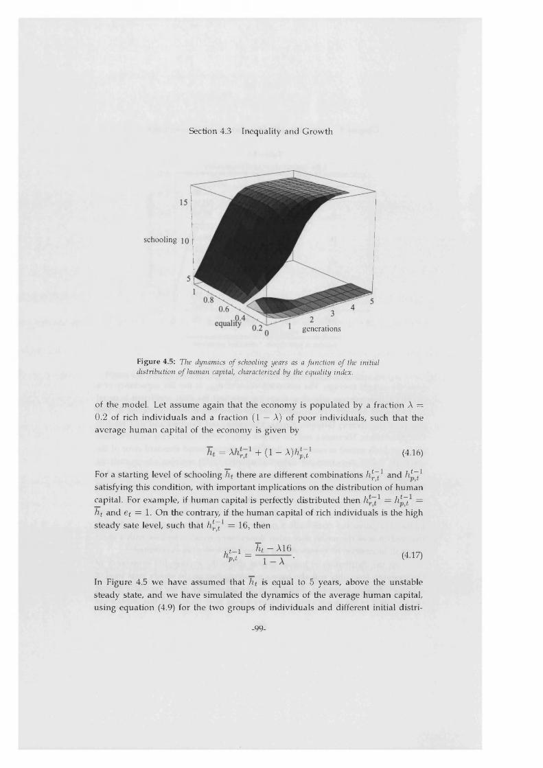
Section 4.3 Inequality and Growth
schooling
Figure 4.5: The dynamics of schooling years as a function of the initial distribution o f human capital, characteñzed by the equality index.
of the model. Let assume again that the economy is populated by a fraction A = 0.2 of rich individuáis and a fraction (1 — A) of poor individuáis, such that the average human capital of the economy is given by
h t = A h t f + (1 - A)fc*y (4.16)
For a starting level of schooling h t there are different combinations h ^ 1 and h l~^ satisfying this condition, with important implications on the distribution of human capital. For example, if human capital is perfectly distributed then h = h l ~̂ = ht and e¿ = 1. On the contrary, if the human capital of rich individuáis is the high steady sate level, such that h ^ 1 = 16, then
, t i h t — A16hv¿¡ = “ I — • (417)
In Figure 4.5 w e have assumed that h t is equal to 5 years, above the unstable steady state, and w e have simulated the dynamics of the average human capital, using equation (4.9) for the two groups of individuáis and different initial distri-
generations
-99-

Chapter 4 Inequality, Life Expectancy and Development
butions, which are characterized by the equality index. Given the calibrated valúes of the parameters, the steady state is reached after five generations or even less. Economies with a low inequality index reach a high steady state in which
= ^p t+ j1 = 16 the transition is more rapid the higher the equality in the initial distribution of hum an capital. In contrast, when < 0.34 the average hum an capital reach very quickly a low steady state in which = 16 andt f+ j - 1 _ QnP,t+j ~ U *
4.4 ConclusionsThis chapter has analyzed an alternative mechanism which explains why inequality in the distribution of income or wealth may be harmful for hum an capital accumulation. The imderlying mechanism is based on the assumption that the life expectancy of individuáis is somehow conditioned by the socioeconomic status of the family which they are bom into. In particular, we have assumed that life expectancy is an increasing function of the hum an capital of the parents, an assumption strongly supported by the empirical evidence.
Based on this assumption the paper develops an overlapping generation model in which individuáis live for sure during their first period of life and face an endogenous probability of surviving the whole second period. Given this probability, they choose the amount of time devoted to accumulating hum an capital that maximizes their intertemporal utility. As expected, the results show that the time individuáis devote to schooling increases with their expected survival probability.
To analyze the relationship between inequality and growth we simúlate a life expectancy function according to the data of schooling years provided by Barro and Lee (2001). The empirical evidence shows a clear relationship between average schooling years and life expectancy. Given the calibrated survival probability function, the model exhibits múltiple steady States depending on initial conditions. Rich individuáis, bom into families whose parents have high levels of education, have high life expectancy. Their long life expectancy encourages them to spend a large number of years in education. On the contrary, individuáis who are bom into poor families have low life expectancy. Accordingly, since the time they expect to enjoy the retums to education is very short, they devote little time to accumulating hum an capital.
These results imply that the initial distribution of education determines the evolution of the aggregate variables in the model. In particular, the model also
-100-

Section 4.5 Appendix 1
shows that inequality may have negative effects upon the growth rate of the economy during the transition to the steady state.
4.5 Appendix 1The optmúzation problem for an individual i is given by
Max u¡= lnc\t + T^í+iC^í-1) ln4 + i (Al.l)L\t
subject to
4 = A L \t + ¡3A{ 1 - L \t ) (A1.2)
6 A4+ 1 = A e x p { a 0 (l - L\t)} - —— - L\t) (A1.3)
L a > 0 (A l .4)
L\t < 1 (A1.5)
The Lagrange function for this problem is as follows:
£ = u\{L\i) + ^ [ l - L \ t] (A1.6)
Applying Kuhn-Tucker conditions for the inequality restriction, the first or- der conditions for this problem are:
^ < o L ‘ > 0 L ‘t | | = 0 (A1.7)
d £ n d £ n— > 0 ^ > 0 ^ = 0
The interior solution (0 < L\t < 1) implies that:
M = 0 m d É | = 0
-101-

Chapter 4 Inequality, Life Expectancy and Development
or
4 - ^ ( 1 -/3) = ̂ [a$A exp{a:0(l - L\t)} - 0Á\ (A1.8)Cit Cit+ 1
Substituting c\t and c\t+1, using (A l.2) and (Al.3) we get
(1 - ¡3) ( exp { a 0 ( l - L¡t)} - —j— TÍ 1 ~ Llt) ) = 7 ^ ‘t+i
H e x p {«0(1 - L\t)} - 0) (L¡t + t ^ t_ u ( 1 - ¿ 4 ) ) (A1-9)V J /
where L¿t is a decreasing function of the expected survival probability.
4.6 Appendix 2Given the valúes of the parameters for the survival probability function, discussed in subsection 4.3.1, when = 0 —► = ^ ̂ hat is, when parentshave no education, offsprings only live during the first period. In such a caseindividuáis face the following optimization problem:
M a x u \= ln¿4 (A2.1)L\t
subject to
4 = AL\t (AZ2)
L¡t > 0 (A2.3)
L\t < 1 (A2.4)
If L\t were not restricted, the optimal valué for L\t w ould tend to infinite. However, the restrictions make the optimal valué take the comer solution of one.It means that individuáis who do not Uve any time in the second period do notaccumulate hum an capital and devote all their time to work in order to maximize their first period consumption.
-102-

Section 4.6 Appendix 2
Otherwise > 0), the optimal valué of L\t is determined by equation(4.9). Nevertheless there are more comer Solutions in this case. In particular, when h \ t l < 3.5 individuáis maximize their utility when L \t = 1, that is, when y\t =
ylt+i = 4 t = 4 + i = A -
-103-

Chapter 5ConclusionsThis thesis has analysed the influence that inequality in the distribution of income and wealth may exert on economic growth rates through three essays. These es- says have focused on this issue from different approaches.
The first essay is in line with the fiscal policy approach. In particular it has extended the theoretical model of Alesina and Rodrik (1994) to allow the govem- ment to finance public spending through labor income taxes. In addition, on the empirical side it has taken into account some differential characteristic from pre- vious work. It has estimated the structural form of the model, has used the most comprehensive income inequality data set available as yet, has used different fiscal variables and, finally, has focused on the countries in which it makes sense to con- trast this approach, that is, countries with democratic regimes and with developed fiscal systems.
The results give scarce empirical support to this approach. Specifically, the variables that work in the political mechanism do not work in the economic mechanism and vice versa. Nevertheless, we also obtained that not only this approach have little support in OECD countries but also the reduced form of the model has no favorable empirical evidence. Similar to the results of Barro (2000), this essay does not find a negative effect from initial inequality in the distribution of income on subsequent economic growth rates in a sample that includes some of the richest countries in the world.
The second essay focuses on the inequality in the distribution of education. Due to the scarcity of an available data set on indicators of inequality in the distribution of education for a broad number of countries and periods, the first goal of this chapter is to take the information on attainment levels provided by the last Barro and Lees (2001) data set and compute Gini coefficients and the distribution of education by quintiles for 108 countries from 1960 to 2000.
The data show that most countries in the sample, with the exception of some advanced countries, have reduced inequality in the distribution of education over the period 1960-2000. Consequently, there has been convergence, instead of polar- ization, in hum an capital Gini coefficients over time. In addition, this new data set allow us to compare the effect of income inequality and education inequality on economic growth. The estimations of cross-section regressions show that the nega-
-104-

tive effect of income inequality on log ran growth rates, found in previous studies, is not robust to the inclusión of regional dummies in the set of explanatory variables. On the contrary, initial distribution of education is negatively related to long run economic growth rates and this relation is robust to the inclusión of regional dummies in the set of explanatory variables and other variables related to education distribution. Moreover, this negative effect also holds with pool data, the exclusión of atypical observations, the use of different inequality indicators and the use of a reduced sample that includes only developing countries. Finally, the data also suggest that the negative relation between education inequality and economic growth is mainly driven through the discouraging effect that education inequality exerts on the investment rates.
The third essay analyses an overlapping generation model that develops a new mechanism that explains why inequality in the distribution of education may reduce average hum an capital accumulation rates in an economy.
The work is based on the assumption that an individuáis life expectancy is conditioned by the family in which she is bom into. In particular, we assume that individuáis bom into rich families will have greater life expectancy than those bom into poor families who are more likely to suffer, for example, from under- nourishment, less hygiene at home or less use of curative and preventive medical Services.
The theoretical model is calibrated with data on average schooling years provided by Barro and Lee (2001) and life expectancy data from the World Bank. The numerical results show múltiple steady states in the evolution of human capital. In particular, there are two stable steady states, a low one with zero years of education an a high one with about 16 years of school. A dynasty converges to the low or high steady state depending on initial conditions. Those individuáis who are bom into poor families have low life expectancy, do not accumulate human capital and work in the production sector for all their lives. Therefore, the higher the number of poor individuáis the lower the average human capital accumulation rates in the economy.
The results of the third essay are similar to the predictions of the human capital and imperfect credit markets approach. Nevertheless, the underlying as- sumptions are different. In these kind of models poor individuáis do not invest in hum an capital because they have some kind of restriction in the credit market. In our model, however, even with perfect credit markets poor individuáis do not invest in hum an capital because their low life expectancy increases the opportunity
-105-

Capítulo 5 Conclusions
cost of becoming educated.On the whole, this thesis has tried to analyse the relation between inequality
and growth from different sides. First, it has gone deeply into the existing political approach. Second, it has analysed empirically the relation between hum an capital inequality and economic growth. Finally, it has developed an altemative channel through which inequality may influence economic growth. Some results have been quite interesting but, however, theses results joint with the conclusions achieved by other contemporaneous papers have raised more unsolved questions.
Firstly, the result in the first paper suggest that inequality in the distribution of income has not exerted a negative effect on the sample of OECD countries. In addition, some figures suggest that this effect could be even positive. On this matter, Barro (2000) finds a positive relation between inequality and growth in rich countries. Therefore, these results arise the following question: does inequality af- fect growth differently in rich and poor countries?.
Secondly, in the second paper we find that the log run effect from initial inequality in the distribution of income on economic growth rates is not robust to the inclusión of other variables in the set of regressors, such as regional dummies. However, the long run negative effect from initial inequality in the distribution of education on economic growth seems to be robust. Moreover, Deiniger and Squire (1998) compare the effect of income inequality and land inequality on long run growth rates. They also find that the effect of land inequality is more robust than that of income inequality. These results emerge the question: why income and wealth inequality may affect differently long run growth rates?.
Although there are some questions not completely understood. The results of this thesis suggest that education inequality has exerted a negative influence on long run growth rates. Those countries that started with greater inequality in the distribution of education in 1960 have grown, on average, a t lower rates than those with a more even distribution. This evidence is in line with the predictions of the new approach, analyzed in the fourth chapter, and with the predictions of some models related to the credit markets and hum an capital investment mechanism.
-106-


References
ReferencesAghion, P. and P. Bolton (1997): “A Theorv of Trickle-Down Growth and Development” .
Review of Economic Studies, 64, 151-172.Aghion, R, E. Caroli and C. García-Peñalosa (1999). "Inequality and Economic
Growth: The Perspective of the New Growth Theories". Journal of Economic Literature, 37, 1615-1660.
Alesina, A. and D. Rodrik (1994). "Distributive Politics and Economic Growth".Quarterly Journal of Economics, 109, 465-490.
Alesina, A. and R. Perotti (1996). "Income Distribution, Political Instability, and Investment". European Economic Remezo, 40,1203-1228.
Azariadis C. (2001): “The Theory of Poverty Traps: W hat Have we Learned” . Mimeo, UCLA.
Banerjee, A. V. and E. Duflo (2000). "Inequality and Growth: W hat Can the Data Say?". NBER WP no. 7793.
Banerjee, A. V. and A. F. Newman (1993): “Occupational Choice and the Process of Development” . Journal of Political Economy, 101(2), 274-298.
Barker, D. (1997): “Maternal Nutrition, Fetal Nutrition and Diseases in Later Life” .Nutrition, 13(9), 807-813.
Barro, R. J. (1990). "Governm ent Spending in a Simple Model of Endogenous Growth".Journal of Political Economy, 98, 103-125.
Barro, R. J. (2000). "Inequality and Growth in a Panel of Countries". Journal of Economic Growth, 5, 5-32.
Barro, R. J. and J. W. Lee (1994): “Data Set for a Panel of 138 Countries." Mimeo.(http:/ / www.nber.org/pub/barro.lee/readm e.txt).
Barro, R. J. and J. W. Lee (1996). “International Measures of Schooling Years and Schooling Quality” . American Economic Review 86 (2), 218-223.
Barro, R. J. and J. W. Lee (2001): “International Data on Educational Attainment Updates and Implications." Oxford Economic Papers, no. 3, pp. 541-63.
Benabou, R. (1996): “Inequality and Growth” . NBER Working Paper, no. 5658.Bertola, G. (1993). "Factor Shares and Savings in Endogenous Growth". American
Economic Review, 83,1184-1199.Birdsall, N. and J. L. Londoño (1997). “Asset Inequality Matters: An Assessment of
the World Banks Approach to Poverty Reduction” . American Economic Review 87 (2), 32-37.
Blackbum K. and G. P. Cipriani (2002): “A Model of Longevity, Fertility and Growth” .
-107-
References
Journal of Economic Dynamics and Control, 26(2), 187-204.Boscá, J. E., M. Fernández and D. Taguas (1997). "Estructura Impositiva en los
Países de la OCDE". Mimeo, DGAPP, Ministerio de Economía y Hacienda.Case, A. D. Lubotsky and Ch. Paxon (2001): “Economic Status and Health in
Childhood: the Origins of the Gradient” . Mimeo, Princeton University.Caselli, F., G. Esquivel and F. Lefort (1996): “Reopening the Convergence Debate:
A New Look at Cross-Country Growth Empirics." Journal of Economic Growth, 1(3), 363-89.
Chari, V. V. and P. J. Kehoe (1999). "Optim al Fiscal and Monetary Policy". NBER Working Paper, no. 6891.
Checchi, D. (2000)."Does Educational Achievement Help to Explain Income Inequality, Mimeo.
Clarke, G. R. G. (1995). "M ore Evidence on Income Distribution and Growth". Journal of Development Economics, 47, 403-427.
Currie, J. and R. Hyson (1999). "Is the Impact of Health Shocks Cushioned by Socioeconomic Status? The Case of Low Birthweight." American Economic Review, 89(2), 245-250.
De la Croix, D. and O. Licandro (1999): “Life Expectancy and Endogenous Growth” . Economic Letters, 65, 255-263.
De la Fuente, A. and R. Doménech (2001): “Human Capital in Growth Regressions: How Much Difference Does Data Quality Make?” . Economics Department Working Papers, no. 262. OECD.
De la Fuente, A. and R. Doménech (2001): “Schooling Data, Technological Dif- fusion and the Neoclasical Model." American Economic Review, Papers and Proceedings, 91(2), 323-27.
Dabán, T., R. Doménech and C. Molinas (1997). "International and Intertempo- ral Comparisons of Real Product in OECD Countries: A Growth Sensitive Analysis". Review of Income and Wealth, 43, 33-48.
Deininger, K. and L. Squire (1996). "A New Data Set Measuring Income Inequality". World Bank Economic Review, 10, 565-591.
Deininger, K.and L. Squire (1998). "N ew Ways of Looking at Oíd Issues: Inequality and Growth". Journal of Development Economics, 57, 259-287.
Díaz-Giménez, J., V. Quadrini and J. V. Ríos-Rull (1997). "Dimensions of Inequality: Facts on the U.S. Distributions of Eamings, Income, and Wealth". Federal Reserve Bank of Minneapolis Quarterly Review, 21, 3-21.
Ehrlich I. and F. T. Lui (1991): “Intergenerational Trade, Longevity, and Economic
-108-

References
Growth” . Journal of Political Economy, 99,1029-1059.Eicher, T. O. and C. García-Peñalosa (2001): “Inequality and Growth: the Dual
Role of Hum an Capital in Development” . Journal of Development Economics, 66, 173-197.
Fields, G. (1989). "A Compendium of Data on Inequality and Poverty for Develo- ping World". Mimeo, Cornell University.
Forbes, J. K. (2000). "A Reassessment of the Relationship Between Inequality and Growth". American Economic Review, 90, 869-887.
Galor, O. and D. Tsiddon (1997). “ The Distribution of Hum an Capital and Economic Growth". Journal of Economic Growth 2, 93-124.
Galor, O. and J. Zeira (1993). "Income Distribution and Macroeconomics". Review of Economic Studies, 60, 35-52.
García-Peñalosa, C. (1994). "Inequality and Growth: A Note on Recent Theories". Investigaciones Económicas, 18, 97-116.
Glomm, G. and B. Ravikumar (1992). “Public versus Prívate Investment in Human Capital: Endogenous Growth and Income Inequality” . Journal of Political Economy 100 (4), 818-834.
Grandmont, J. M. (1978). "Intermediate Preferences and the Majority Rule". Econo- metrica, 46, 317-330.
Islam, N. (1995). “Growth Empirics: A Panel Data Approach” . Quarterly Journal of Economics, CX, 1127-1170.
Jain, S. (1975). "Size Distribution of Income: A Compilation of Data". Washington, DC: World Bank.
Jones, L. E., R. E. Manuelli and P. E. Rossi. (1993). "Optim al Taxation in Models of Endogenous Growth". Journal of Political Economy, 101, 485-517.
Judd, K. L. (1985). "Redistributive Taxation in a Simple Foresight Model". Journal of Public Economics, 28, 59-83.
Kalemli-Ozcan, D. (2001): "Does Mortality Decline Promote Economic Growth?". Mimeo, University of Houston.
Kalemli-Ozcan, S ., H. E. Ryder and D. N. Weil (2000): “Mortality Decline, H um an Capital Investment and Economic Growth” . Journal of Development Economics, 62, 1-23.
Krueger, A. B. and M. Lindahl (2001): “Education for Growth: W hy and for Whom?” . Journal of Economic Literature, 39(4), 1101-1136.
Krusell, P , V. Quadrini and J. V. Ríos-Rull (1997). "Politico-economic equilibrium and economic growth". Journal of Economic Dynamics and Control, 21, 243-272.
-109-

References
Kuznets, S. (1955). “Economic Growth and Income Inequality” . American Economic Review 45 (1), 1-28.
Lee, K., M. H. Pesaran and R. Smith (1997): ‘Growth and Convergence in a Multi-Country Empirical Stochastic Solow Model." Journal of Applied Econometrics,12(4), 357-392.
Lee, K., M. H. Pesaran and R. Smith (1998): ‘Growth Empirics: A Panel Data Approach - A Comment." Quarterly Journal of Economics, 113(1), 319-323.
Lee, W.and J. E. Roemer (1998). "Income Distribution, Redistributive Politics, and Economic Growth". Journal of Economic Growth, 3, 217-240.
Levine, R. and D. Renelt (1992). "A sensitivity Analysis of Cross-Country Growth Regressions". American Economic Review, 82, 942-963.
Li, H., L. Squire and H. Zou (1998). “Explaining International and Intertemporal Variations in Income Inequality” . The Economic Journal, 108, 26-43.
López, R., V. Thomas and Y. Wang (1998). “Addressing the Education Puzzle. The Distribution of Education and Economic Reforms” . World Bank Working Papers, no. 2031.
Mankiw, N., D. Romer and P. Weil (1992). "A Contribution to the Empirics of Economic Growth". Quarterly Journal of Economics, 107, 407-437.
Marmot, M. G., G. D. Smith, S. Stansfeld, C. Patel, F. North, J. Head, I. White,E. Brunner and A. Feeney. (1991): “Health Inequality Among British Civil Servants: the Whitahall II Study” . The Lancet, 337, 1387-1393.
Mincer, J. (1974): Schooling, Experience and Eamings. Columbia University Press.Moav, O. (2001): “Cheap Children and the Persistence of Poverty” . CEPR Discus-
sion Paper Series, no. 3059.Partridge, M. D. (1997). "Is Inequality Harmful for Growth? Comment". American
Economic Review, 87, 1019-1032.Paukert, F. (1973). "Income Distribution at Different Levels of Development: A
Survey of Evidence". International Labour Review, 108, 97-125.Perotti, R. (1996). "Growth, Income Distribution and Democracy: W hat Data Say".
Journal of Economic Growth, 1,149-187.Persson, T. and G. Tabellini (1994). "Is Inequality Harmful for Growth? Theory
and Evidence". American Economic Review, 84, 600-621.Piketty, T. (1997): “The Dynamics of the Wealth Distribution and the Interest Rate
with Credit Rationing” . Review of Economic Studies, 64,173-189.Quah, D. (1993). “Galton's Fallacy and Test of the Convergence Hypothesis” . Scan-
dinavian Journal of Economics 95(4), 427-443.
-110-

References
Quah, D. (1996). “Empirics for Economic Growth and Convergence” . European Economic Review, 40,1353-1375.
Ravelli, A., J. van der Meulen, R. Michels, C. Osmond, D. Barker, C. Hales and O. Bleker (1998): “Glucose Tolerance in Adults after Prenatal Exposure to Famine” . The Lancet, 351,173-177.
Saint-Paul, G. and T. Verdier (1993). "Education, Democracy and Growth". Journal of Development Economics, 42, 399-407.
Smith, J. P. (1999): “Healthy Bodies and Thick Wallets: The Dual Relation Between Health and Economic Status” . Journal of Economic Perspectives, 13, 145-166.
Smith, V. K., D. H. Taylor, Jr., and F. A. Sloan (2001): “Longevity Expectations and Death: Can People Predict Their Own Demise?” . American Economic Review, 91(4), 1126-1134.
Soares, R. R. (2001):"Life Expectancy, Education Attainment, and Fertility Choice". Mimeo, University of Chicago.
Tallman, E. W. and P. Wang (1994). “Human Capital and Endogenous Growth. Evidence from Taiwan” . Journal ofMonetary Economics, 34,101-124.
Tamura, R. (2002):"Human Capital and Economic Development". Working Paper No. 2002-5, Federal Reserve Bank of Atlanta.
Tanzi V. (1998). "Fundam ental Determinants of Inequality and the Role of Government". IMF Working Paper, 98/178.
Thomas, V., Y. Wang, and X. Fan (2000): “Measuring Education Inequality: Gini Coefficients of Education." Mimeo. The World Bank.(http: / / econ.worldbank.org/ files/1341_wps2525.pdf.)
Wadsworth, M. and D. Kuh (1997): “Childhood Influences on Adult Health: A Review of Recent Work from the British 1946 National Birth Cohort Study, the MRC National Survey of Health and Development” . Pediatric and Perinatal Epidemiólogo, 11, 2-20.
Ware, J. A. Davies-Avery and C. Donald (1978): “General Health Perceptions” . R- 1987/5 HEW, RAND. Santa Monica, California.
-111-


Resumen
Resumen
Tercer capítulo
A n te c e d e n te sGran parte de los trabajos teóricos que analizan la relación entre desigualdad y crecimiento hacen referencia a la desigualdad en la distribución de activos en la economía. En particular, en el trabajo teórico que se analiza en el primer capítulo, enmarcado en el enfoque político, los individuos difieren en sus dotaciones iniciales de capital. Del mismo modo, la distribución de la riqueza también es la base del enfoque de imperfecciones en el mercado de crédito ya que, asumiendo indivisibilidad en los proyectos de inversión, aquellos individuos cuya riqueza es inferior al coste del proyecto no podrán realizar su inversión si tienen limitado su acceso al mercado de crédito. Sin ambargo, la falta de datos sobre distribución de la riqueza para un amplio número de países y períodos ha llevado a la mayor parte de trabajos empíricos que analizan el efecto de la desigualda sobre el crecimiento a utilizar datos sobre distribución de la renta como proxy de la distribución de la riqueza. Algunas excepciones son los trabajos de Alesina y Rodrik (1994) o Deininger y Squire (1998) en los que se incluye la distribución de la tierra para aproximar la distribución de la riqueza. No obstante, la tierra puede ser un indicador insuficiente de la riqueza ya que hay otros componentes como, por ejemplo, el capital humano, que pueden ser importantes determinantes de la riqueza y, a su vez, de las tasas de crecimiento de una economía.
O b je tiv oEl primer objetivo del tercer capítulo es calcular una base de datos sobre distribución de la educación para un gran número de países y para un amplio período de tiempo. Posteriormente, se pretende analizar la evolución de la desigualdad en la distribución de la educación a lo largo del tiempo y comparar dicha evolución entre los distintos países que componen la muestra. Finalmente, el objetivo de este capítulo es utilizar los nuevos indicadores de desigualdad en la distribución de la educación para ver su efecto sobre las tasas de crecimiento de los distintos países y comparar los resultados con el efecto de la desigualdad en la distribución de la renta.
-112-

Resumen
D is c u s ió nCon el objetivo de calcular una base de datos sobre desigualdad en la distribución de la educación para un amplio número de países y períodos, en el tercer capítulo se utiliza la base de datos sobre niveles educativos de Barro y Lee (2001) y se calculan índices de Gini de distribución de la educación para 108 países en el período 1960-2000. Además, para ampliar la información que proporciona el índice de Gini, también se ha calculado la distribución de la educación por quintiles.
C o n c lu s io n e sUtilizando estos indicadores de desigualdad las principales conclusiones del capítulo son las siguientes. Primera, al analizar la evolución de los indicadores de desigualdad a lo largo del tiempo se observa un proceso de convergencia en los índices de Gini de los países que componen la muestra. Este hecho se debe a que, por una parte, la gran mayoría de países han reducido la desigualdad en la distribución de la educación a lo largo del período y, por otra, algunos de los países que partían con distribuciones de la educación más igualitarias en 1960, como por ejemplo Nueva Zelanda, Hungría, Finlandia, Holanda o Gran Bretaña, han incrementado la desigualdad durante el período 1960-2000. Segunda, en la estimación de ecuaciones de crecimiento, el índice de Gini de la distribución de la educación presenta resultados más robustos que el índice de Gini de la distribución de la renta. El efecto negativo de la desigualdad inicial en la distribución de la renta sobre las tasas de crecimiento de la renta per cápita de largo plazo, obtenido en trabajos previos, desaparece cuando en el conjunto de variables explicativas se incluyen variabes ficticias que recogen características específicas de las distintas regiones que componen la muestra. Por el contrario, se obtiene un efecto negativo de la desigualdad inicial en la distribución de la educación sobre las tasas de crecimiento de la renta per cápita de largo plazo que es robusto a la inclusión de variables ficticias regionales y a la inclusión de otras variables correlacionadas con la distribución de la educación como, por ejemplo, los años medios de escolarización. Además, los resultados se mantienen con la utilización de distintas muestras o distintas variables que miden la distribución de la educación de una economía. Finalmente, las estimaciones sugieren que gran parte del efecto negativo que la desigualdad en la distribución de la educación tiene sobre las tasas de crecimiento se debe a la relación negativa existente entre la desigualdad de la educación y la acumulación de factores de la economía.
-113-

Resumen
Cuarto capítuloAntecedentesAlgunos trabajos empíricos han incluido a la esperanza de vida entre los determinantes importantes de las tasas de crecimiento de las economías. Es por ello que, actualmente están surgiendo modelos teóricos en los que la esperanza de vida es una de las principales variables que determinan la elección endógena de fertilidad y la acumulación de capital humano de los individuos. Por otra parte, en el tercer capítulo se encuentra una alta correlación entre la esperanza de vida y la desigualdad en la distribución de la educación.
ObjetivoEn el capítulo cuarto se analiza un modelo teórico que estudia la relación entre desigualdad en la distribución de la educación, esperanza de vida y acumulación de capital humano. El objetivo es encontrar un modelo teórico que explique por qué los países con mayor desigualdad en la distribución de la educación tienen menor esperanza de vida y, a su vez, menor acumulación promedio de capital humano.
DiscusiónEn el cuarto capítulo se plantea un modelo de generaciones solapadas en el que los individuos viven con certeza un primer período y tienen una probabilidad endógena de sobrevivir durante el segundo período. En este modelo se supone que la probabilidad de sobrevivir durante el segundo período depende de la familia en la que un individuo nace. Dada su esperanza de vida, el individuo elige los años de escolarización que maximizan su función de utilidad intertemporal. El modelo se calibra con datos sobre años medios de escolarización y esperanza de vida de distintos países.
ConclusionesTras calibrar el modelo de acuerdo con los datos, los resultados numéricos indican la existencia de múltiples estados estacionarios en la evolución de la educación a lo largo del tiempo. En particular se obtienen dos estados estacionarios estables, uno bajo donde los individuos no acumulan capital humano y otro alto con 16 años de escolarización. El modelo refleja la realidad de muchos países de América Latina, sur de Asia o África Sub-Sahariana en los que muchos individuos nacidos en familia pobres cuyos padres son analfabetos, viven un escaso período de tiempo,
-114-

Resumen
no dedican tiempo a acumular capital humano y trabajan como trabajadores no cualificados durante sus cortéis vidas.
-115-
