University of Calgary

PRISM: University of Calgary's Digital Repository

Graduate Studies The Vault: Electronic Theses and Dissertations

2016

Three Essays in Financial Economics

Isakin, Maksim

Isakin, M. (2016). Three Essays in Financial Economics (Unpublished doctoral thesis). University

of Calgary, Calgary, AB. doi:10.11575/PRISM/28438

http://hdl.handle.net/11023/3044

doctoral thesis

University of Calgary graduate students retain copyright ownership and moral rights for their

thesis. You may use this material in any way that is permitted by the Copyright Act or through

licensing that has been assigned to the document. For uses that are not allowable under

copyright legislation or licensing, you are required to seek permission.

Downloaded from PRISM: https://prism.ucalgary.ca

UNIVERSITY OF CALGARY

Three Essays in Financial Economics

by

Maksim Isakin

A THESIS SUBMITTED TO THE FACULTY OF GRADUATE STUDIES

IN PARTIAL FULFILLMENT OF THE REQUIREMENTS

FOR THE INTERDISCIPLINARY DEGREE OF DOCTOR OF PHILOSOPHY

GRADUATE PROGRAM IN ECONOMICS

and

GRADUATE PROGRAM IN MANAGEMENT

CALGARY, ALBERTA

June, 2016

c� Maksim Isakin 2016

Abstract

This dissertation consists of three essays on financial economics. In the first essay, I build a theo-

retical model for pricing collateralized debt obligations (CDO) based on varying precision of credit

ratings. A credit rating agency (CRA) produces noisy ratings to maximize the proportion of firms

with high ratings but still ensures that firms choose lower risk projects. Increased fundamental

volatility in bad times makes high-risk choices more appealing to firms, which the CRA responds

to by increasing the precision of ratings. Only firms that can call existing bonds and issue new

ones will choose low risk projects at such times. Therefore, the resulting high risk strategy for

constrained firms in such periods implies that junior tranches get seriously impacted. In contrast,

senior tranches are more exposed to growth shocks, which increase the risk of all firms’ projects.

I structurally estimate the parameters of the model and show that the model is able to explain the

levels and a significant fraction of the volatilities of CDO tranche spreads. In the second essay, I

take the user cost approach to modelling a banking firm and analyze banks’ optimal response to

monetary and regulatory changes. The bank maximizes its profit choosing the quantities of finan-

cial goods such as deposits, loans, and investments based on their user costs. I estimate the system

of demand and supply of financial goods using data on U.S. banks over the 1992-2013 period. The

policy tools change the user costs of the financial goods and, therefore, bank’s demand and supply

of financial goods. I report the effects of an increase in interest paid on reserves, federal funds

rate and others. In the third essay, I develop a framework for estimating demand systems with

autoregressive conditional heteroscedasticity (ARCH). In this setup, the conditional variance is a

random variable depending on current and past information. Since most economic and financial

time series are nonlinear, using parametric nonlinear demand systems with an ARCH-component

can significantly improve the quality of a model. I prove the invariance of the maximum likelihood

estimator with respect to the choice of an estimated demand subsystem.

ii

Acknowledgements

I would like to express my gratitude to my supervisor, Professor Apostolos Serletis, who has helped

me throughout this entire venture with his guidance and insightful remarks. I thank him for his

continuous willingness to help with every step. It was my pleasure to work with him.

I would like to thank my co-supervisor, Professor Alexander David, for whom my admiration

and respect are enormous. Without him this research would have been most difficult. His constant

advice and support have been essential in my development as a researcher.

I also wish to thank Joanne Roberts, Kenneth James McKenzie, Kunio Tsuyuhara, Curtis Eaton,

Jean-Francois Wen for their guidance and helpful discussions.

I would like to thank my mother Tatiana Isakina and my father Aleksandr Isakin for encourag-

ing my interest in economics, for their patience and sense of humour. I thank my sister Ekaterina

Isakina for her support and long discussions of my papers.

Finally, I would like to thank my wife Alena Isakina for her belief in me. She has shared all

difficult and happy moments in my research.

iii

Table of Contents

Abstract . . . . . . . . . . . . . . . . . . . . . . . . . . . . . . . . . . . . . . . . . . . iiAcknowledgements . . . . . . . . . . . . . . . . . . . . . . . . . . . . . . . . . . . . iiiTable of Contents . . . . . . . . . . . . . . . . . . . . . . . . . . . . . . . . . . . . . . ivList of Tables . . . . . . . . . . . . . . . . . . . . . . . . . . . . . . . . . . . . . . . . viList of Figures . . . . . . . . . . . . . . . . . . . . . . . . . . . . . . . . . . . . . . . . vii1 Credit Ratings, Credit Crunches,

and the Pricing of Collateralized Debt Obligations . . . . . . . . . . . . . . . . . . 21.1 Introduction . . . . . . . . . . . . . . . . . . . . . . . . . . . . . . . . . . . . . . 21.2 Model . . . . . . . . . . . . . . . . . . . . . . . . . . . . . . . . . . . . . . . . . 71.3 Equilibrium . . . . . . . . . . . . . . . . . . . . . . . . . . . . . . . . . . . . . . 10

1.3.1 Belief Updating From Learning and Bayesian Persuasion . . . . . . . . . . 161.4 Securitized Debt . . . . . . . . . . . . . . . . . . . . . . . . . . . . . . . . . . . . 171.5 Empirical Analysis . . . . . . . . . . . . . . . . . . . . . . . . . . . . . . . . . . 19

1.5.1 First Stage Maximum Likelihood Estimation of Regime Switching Model . 191.5.2 Second Stage SMM Estimation of Firms’ Project Return Parameters . . . . 211.5.3 Risk-Adjustment Parameters . . . . . . . . . . . . . . . . . . . . . . . . . 221.5.4 The Credit Spreads Puzzle, Spread Dynamics, and the Convexity Effect . . 22

1.6 Data Description . . . . . . . . . . . . . . . . . . . . . . . . . . . . . . . . . . . 241.7 Conclusion . . . . . . . . . . . . . . . . . . . . . . . . . . . . . . . . . . . . . . 25Bibliography . . . . . . . . . . . . . . . . . . . . . . . . . . . . . . . . . . . . . . . . 382 User Costs, the Financial Firm, and Monetary

and Regulatory Policy . . . . . . . . . . . . . . . . . . . . . . . . . . . . . . . . . 412.1 Introduction . . . . . . . . . . . . . . . . . . . . . . . . . . . . . . . . . . . . . . 412.2 The User Cost Approach . . . . . . . . . . . . . . . . . . . . . . . . . . . . . . . 442.3 The Variable Profit Function Approach . . . . . . . . . . . . . . . . . . . . . . . . 472.4 Flexible Functional Forms . . . . . . . . . . . . . . . . . . . . . . . . . . . . . . 49

2.4.1 The Translog . . . . . . . . . . . . . . . . . . . . . . . . . . . . . . . . . 492.4.2 The Normalized Quadratic . . . . . . . . . . . . . . . . . . . . . . . . . . 512.4.3 The Generalized Symmetric Barnett . . . . . . . . . . . . . . . . . . . . . 55

2.5 Data and Measurement Matters . . . . . . . . . . . . . . . . . . . . . . . . . . . . 572.6 Econometric Issues . . . . . . . . . . . . . . . . . . . . . . . . . . . . . . . . . . 612.7 Empirical Evidence . . . . . . . . . . . . . . . . . . . . . . . . . . . . . . . . . . 64

2.7.1 Theoretical Regularity . . . . . . . . . . . . . . . . . . . . . . . . . . . . 642.7.2 Elasticities of Transformation . . . . . . . . . . . . . . . . . . . . . . . . 662.7.3 Compensated Price Elasticities . . . . . . . . . . . . . . . . . . . . . . . . 67

2.8 Monetary and Regulatory Policy Analysis . . . . . . . . . . . . . . . . . . . . . . 692.8.1 Interest on Reserves . . . . . . . . . . . . . . . . . . . . . . . . . . . . . 692.8.2 Reserve Requirements . . . . . . . . . . . . . . . . . . . . . . . . . . . . 702.8.3 Changes in the Federal Funds Rate . . . . . . . . . . . . . . . . . . . . . . 702.8.4 Changes in the Return on Investments . . . . . . . . . . . . . . . . . . . . 71

2.9 Conclusion . . . . . . . . . . . . . . . . . . . . . . . . . . . . . . . . . . . . . . 72Bibliography . . . . . . . . . . . . . . . . . . . . . . . . . . . . . . . . . . . . . . . . 103

iv

3 Stochastic Volatility Demand Systems . . . . . . . . . . . . . . . . . . . . . . . . 1073.1 Introduction . . . . . . . . . . . . . . . . . . . . . . . . . . . . . . . . . . . . . . 1073.2 Neoclassical Demand Theory . . . . . . . . . . . . . . . . . . . . . . . . . . . . . 1083.3 Stochastic Volatility Demand Systems . . . . . . . . . . . . . . . . . . . . . . . . 1103.4 A Specific Case . . . . . . . . . . . . . . . . . . . . . . . . . . . . . . . . . . . . 1123.5 Empirical Application . . . . . . . . . . . . . . . . . . . . . . . . . . . . . . . . . 1153.6 Conclusion . . . . . . . . . . . . . . . . . . . . . . . . . . . . . . . . . . . . . . 118Bibliography . . . . . . . . . . . . . . . . . . . . . . . . . . . . . . . . . . . . . . . . 121

v

List of Tables

1.1 What Explains CDO Tranche Spreads? . . . . . . . . . . . . . . . . . . . . . . . 271.2 Maximum Likelihood Estimates of 4-Regime Markov Switching Model for Ratio

of Credit Growth at Nonfinancial Firms to GDP and Real GDP Growth . . . . . . 281.3 Second Stage SMM Estimation of Firms’ Project and Risk Adjustment Parameters 291.4 Implied Spreads (In Basis Points) From SMM Parameter Estimates . . . . . . . . 29

2.1 Size distribution of U.S. banks . . . . . . . . . . . . . . . . . . . . . . . . . . . . 752.2 Assets and liabilities of U.S. banks (in billions) . . . . . . . . . . . . . . . . . . . 762.3 Percentage of Observations When Financial Goods are Outputs . . . . . . . . . . . 772.4 User Costs Averaged Across Banks (and the Discount Rate) . . . . . . . . . . . . 782.5 Translog Parameter Estimates . . . . . . . . . . . . . . . . . . . . . . . . . . . . . 792.6 Normalized Quadratic Parameter Estimates . . . . . . . . . . . . . . . . . . . . . 802.7 Generalized Barnett Parameter Estimates . . . . . . . . . . . . . . . . . . . . . . 812.8 Elasticities of Transformation, All Banks . . . . . . . . . . . . . . . . . . . . . . . 832.9 Elasticities of Transformation, Banks With Assets Less Than $100 Million . . . . . 842.10 Elasticities of Transformation, Banks With Assets Between $100 Million and $1

Billion . . . . . . . . . . . . . . . . . . . . . . . . . . . . . . . . . . . . . . . . . 852.11 Elasticities of Transformation, Banks With Assets Between $1 Billion and $10

Billion . . . . . . . . . . . . . . . . . . . . . . . . . . . . . . . . . . . . . . . . . 862.12 Elasticities of Transformation, Banks With Assets More Than $10 Billion . . . . . 872.13 Price Elasticities, All Banks . . . . . . . . . . . . . . . . . . . . . . . . . . . . . 882.14 Price Elasticities, Banks With Assets Less Than $100 Million . . . . . . . . . . . . 892.15 Price Elasticities, Banks With Assets Between $100 Million and $1 Billion . . . . 902.16 Price Elasticities, Banks With Assets Between $1 Billion and $10 Billion . . . . . 912.17 Price Elasticities, Banks With Assets More Than $10 Billion . . . . . . . . . . . . 92

vi

List of Figures and Illustrations

1.1 Tranche Spreads, Economic Growth, and Credit Availability . . . . . . . . . . . . 301.2 Sequence of Events . . . . . . . . . . . . . . . . . . . . . . . . . . . . . . . . . . 311.3 Belief Updating From Learning and Bayesian Persuasion . . . . . . . . . . . . . . 321.4 Probabilities of the States From Regime Switching Model (1950:Q1 – 2014:Q4) . 331.5 Fundamentals: Data and Fitted From Regime Switching Model (1950:Q1 - 2014:Q4)

. . . . . . . . . . . . . . . . . . . . . . . . . . . . . . . . . . . . . . . . . . . . 341.6 Model and Actual Spreads on Senior and Equity Tranches . . . . . . . . . . . . . 351.7 Distribution of Firms’ Capital Stocks . . . . . . . . . . . . . . . . . . . . . . . . 361.8 Equity Value under the LR and HR Projects . . . . . . . . . . . . . . . . . . . . . 37

2.1 Dynamics of Bank Assets . . . . . . . . . . . . . . . . . . . . . . . . . . . . . . . 932.2 Dynamics of Bank Liabilities . . . . . . . . . . . . . . . . . . . . . . . . . . . . . 942.3 Average Reference Discount Rates . . . . . . . . . . . . . . . . . . . . . . . . . . 952.4 Own-price elasticities for debt securities, hSS . . . . . . . . . . . . . . . . . . . . 962.5 Own-price elasticities for loans and leases, hLL . . . . . . . . . . . . . . . . . . . 972.6 Own-price elasticities for deposits, hDD . . . . . . . . . . . . . . . . . . . . . . . 982.7 Own-price elasticities for other debt, hOO . . . . . . . . . . . . . . . . . . . . . . 992.8 Own-price elasticities for equity, hEE . . . . . . . . . . . . . . . . . . . . . . . . 1002.9 Effects of a 25 Basis Points Increase in the Federal Funds Rate . . . . . . . . . . . 1012.10 Effects of a 25 Basis Points Increase in the Return to Investment . . . . . . . . . . 102

3.1 Squared residuals of equation (22), e21 . . . . . . . . . . . . . . . . . . . . . . . . 119

3.2 Squared residuals of equation (23), e22 . . . . . . . . . . . . . . . . . . . . . . . . 120

vii

Overview

After the 2008 financial crisis, the riskiness of debt markets and efficiency of monetary regulation

have become a focus of attention among academics, policy makers, and practitioners. A large part

of this discussion centres on the role of imperfect credit ratings for debt markets, in particular mar-

kets of structured debt products. An important question is whether information frictions brought

by imperfect credit ratings create additional risk for structured debt securities. Another subject of

ongoing debate is the efficiency of the monetary policy conducted by the Federal Reserve before

and after the crisis. A natural question that arises in this analysis is how monetary and regulatory

changes affect the U.S. banking sector. In this dissertation, I address these questions.

In the first chapter, I develop an equilibrium model with imperfect information to analyze

the pricing and risk of structured finance products. In particular, I explain why senior tranche

spreads are relatively more exposed to macroeconomic growth shocks, while junior spreads are

more exposed to credit availability shocks. In the model, a credit rating agency optimally changes

precision of its credit ratings. The credit ratings affect firm’s cost of capital and create dynamic

incentives for firms to raise or refinance their debt. If the credit market is disrupted, the firms cannot

refinance their debt they may increase their risk-taking according to asset substitution mechanism.

The increased risk of constrained firms in such periods implies that junior tranches get seriously

impacted. In contrast, senior tranches are more exposed to macroeconomic growth shocks, which

increase the risk of all firms’ projects. I structurally estimate the parameters of the model and show

that an endogenously generated ”convexity effect”, in large part due to the time varying precision

of credit ratings, is much more important in understanding CDO tranche spreads than the spread

on the entire pool of firms, the subject of past studies.

The second chapter investigates how monetary policy instruments and financial regulation af-

fect a banking firm. In doing so, I take the user cost approach to determine the value of bank’s

financial goods such as loans, deposits and equity capital. The user cost approach explicitly takes

viii

into account bank’s cost of funds and make bank’s decision problems aligned across financial insti-

tutions. Then I assume that the banking firm is a profit-maximizing entity producing intermediation

services between lenders and borrowers. Since the form of banking technology and profit function

is unknown, I approximate the profit function using three flexible functional forms: translog, nor-

malized quadratic and generalized Barnett. With a particular functional form I derive the system

of demand and supply equations and estimate this system using bank level data.

In the third chapter, I address the estimation of stochastic volatility demand systems. Since the

homoscedasticity assumption is unrealistic for most economic and financial time series, I assume

that the covariance matrix of the errors of demand systems is time-varying and derive the maximum

likelihood estimator. In the model, unconditional variance is constant but the conditional variance,

like the conditional mean, is also a random variable depending on current and past information. I

also prove an important practical result of invariance of the maximum likelihood estimator with

respect to the choice of an equation eliminated from a singular demand system. An empirical

application is provided, using the BEKK specification to model the conditional covariance matrix

of the errors of the basic translog demand system.

Statement of contribution. The paper presented in the first chapter is co-authored with

Alexander David who conducted the first stage of the estimation and described the results in the

introduction and section 1.5 and edited other sections. The papers in the second and third chap-

ters are co-authored with Apostolos Serletis who edited the text and described the results in the

introductions of both papers.

1

Chapter 1

Credit Ratings, Credit Crunches,

and the Pricing of Collateralized Debt Obligations

Joint paper with Alexander David

1.1 Introduction

A typical structured debt product such as a collateralized debt obligation (CDO) is a large pool

of economic assets with a prioritized structure of claims (tranches) against this collateral. These

instruments have made it possible to repackage credit risks and produce claims with significantly

lower default probabilities and higher credit ratings than the average asset in the underlying pool.

The structured finance market demonstrated spectacular growth during the decade before the fi-

nancial crisis of 2007/08 but almost dried up following massive downgrades and defaults of highly

rated structured products during the crisis (see Coval, Jurek and Stafford (2009b)). In an influential

paper, Coval, Jurek and Stafford (2009a) argue that investors did not adequately price the risk in

senior CDO tranches prior to the financial crisis (see also Collin-Dufresne, Goldstein and Yang

(2012) and Wojtowicz (2014)). In this paper, we do not focus on mispricing at particular points

of time, but provide a new theoretical model, which is based on the dynamic information content

of credit ratings through macroeconomic and credit cycles. We then structurally estimate the pa-

rameters of this model, and show that it is able to explain a substantial proportion of the historical

variation in CDO tranche spreads.

Following the work by these above authors, we study the time series of spreads on tranches on

the Dow Jones North American Investment Grade Index of credit default swaps, which are shown

in Figure 1.1. The “equity” tranche (top-left panel) represents the 0 to 3 percent loss attachment

2

points (these securities suffer losses if the loss on the entire collateral pool is between 0 and 3

percent of the underlying capital, are wiped out if the losses exceed 3 percent), while the “senior”

tranche (top-right panel) represents the 15 to 100 loss attachment points. While both spread series

rose rapidly during the financial crisis, the rise in the senior tranche spread was more spectacular,

from only about 10 basis points (b.p.) before the crisis, to above 230 b.p. at its peak. The equity

tranche by comparison, only roughly doubled from its pre-crisis level of 1175 b.p to 2700 b.p. at its

highest point. Post-crisis (2012-2014), the senior tranche spread was still 27 b.p., while the equity

tranche spread returned to its pre-crisis level.

The bottom-left panel of Figure 1.1 shows the quarterly growth in real GDP between 2004 and

2014. As seen, GDP growth bottomed out in the middle of the great recession, and resumed at a

more normal pace soon after the recession. The bottom-right panel shows that the ratio of credit

growth at nonfinancial companies to nominal GDP fell through the recession, and only bottomed

out after 2-3 quarters of the end of the recession. Matching up with the tranche spreads in the top

panels, the figures suggest that the senior tranche was more affected by the fluctuations in growth,

while the equity tranche was more affected by credit growth fluctuations. We examine if this is

true with some simple regressions.

In Table 1.1, we regress the spread on the entire pool (CDX) as well as different tranche spreads

on the two fundamentals. For each of the spread series, it is noteworthy that despite the presence of

a macroeconomic factor, credit growth additionally impacts tranche spreads. However, the relative

importance of the two fundamentals for junior and senior spreads is quite different. In lines 4 to

6, we see that GDP growth only explains only about 14.5 percent of the variation in the equity

tranche spread, while credit growth explains nearly 51 percent of its variation. Both variables are

significant in a joint regression. In contrast, in lines 13 to 15, we see that GDP growth explains

56 percent of the variation in the senior tranche spread, but credit growth explains only about 18

percent. In this paper, we ask why the relative exposure of the junior and senior tranches to the

alternative shocks is so different, and provide a new model to explain it.

3

There are three crucial ingredients in our model. First, we endogenize the risk of the firms

using an asset substitution mechanism. In particular, firms optimally choose their risk based on the

amount of debt that they need to service. Second, we introduce imperfect credit ratings using the

Bayesian persuasion concept, which we discuss more completely below. This concept implies that

the rating agency changes the intensity of its investigation of firms’ credit quality with the goal

of maximizing the proportion of firms with high credit ratings. Finally, credit availability in the

model can be in “available” or “nonavailable” states.

These features generate a mechanism that amplifies and propagates macroeconomic shocks

and can create catastrophic risk observed in the prices of CDO tranches (see Collin-Dufresne et al.

(2012)). According to this mechanism the rating agency produces a noisy signal (ratings) that al-

lows the firms to borrow at the cost compatible with low-risk behaviour, i.e. the credit ratings abate

the moral hazard problem just enough to induce low-risk behavior in current economic conditions.

In a sense, this puts the firms on the edge of low-risk and high-risk technologies and if economic

conditions change the firms could switch to risky behavior. To prevent this switching the rating

agency steps in and produces more precise signal (ratings). The new ratings can decrease the cost

of borrowing for the firms to maintain low-risk behavior, if they can call existing debt. However, if

credit availability is off, then, firms cannot call existing debt and will continue to choose high risk

projects.

We incorporate these features into a model of CDO tranches, where firms’ bonds are pooled

each period, and provide returns over 5 years, broken up in a short initial period of 1 year, after

which the bonds can be called, and a longer period of 4 years, at the end of which the returns are

distributed. In our model, we study how the information in credit ratings evolve over the business

cycle and the pricing consequences of these dynamics. We apply our model to explain risk and

pricing dynamics of the different CDO tranches. In particular we shed light on the difference in

relative exposure of junior and senior tranches to macro and credit availability shocks.

Our paper builds on the coordinating role of rating agencies in driving better investment deci-

4

sions by firms as in Boot, Milbourn and Schmeits (2006) and Manso (2013).1 In both papers the

models exhibit multiplicity of equilibria and the credit rating agency plays a coordinating role. In

their work, ratings lower the cost of finance specially since certain classes of investors are forced

by institutional rigidities to invest in highly rated securities. We instead build on the concept of

Bayesian persuasion (exemplified in a litigation context in Kamenica and Gentzkow (2011)), in

which the precisions of the ratings are controlled by the rating agencies investigation process. In

good times, the agencies allow some degree of contamination of the good ratings class by con-

ducting a less thorough examination of firms credit quality, but still ensuring that the overall cost

of capital of the mix of firms is low enough to induce the low risk project choice by high quality

firms. In periods of deteriorating fundamentals, the quality of the ratings are improved to weed

out bad firms from the high rating class, so that once again good quality firms still purse low risk

projects. Overall, the procedure maximizes the amount of debt with high ratings. It is important

to note that the time varying quality of ratings is distinct from alternative rating agency behaviors

such as misreporting and ratings inflation (see e.g. Fulghieri, Strobl and Xia (2014)), which might

also have played a role in financial crisis.

A significant contribution of our paper is a structural estimation of our Bayesian persuasion

model. Our estimation proceeds in two stages. At the first stage we use standard maximum likeli-

hood of regime switching models (see Hamilton (1994)) to estimate the cycles in credit availability

and macroeconomic growth. The regimes are observed by the agents in the model, but are unob-

served by the econometrician. In the second stage, we use the simulation method of moments

(SMM) to estimate the parameters of firms’ projects that fit tranche spreads. Our estimated model

provides several insights. In the model, during credit nonavailability states, several firms cannot

refinance their existing debt, and hence, they choose HR projects. Therefore an increase in risk of

some firms (relative to credit availability states) implies that the chance of the equity tranches ex-

periencing significant losses increases. But, since all firms do not increase their risk, the chance of1We therefore have a coordination game with strategic complementarity as for example in Milgrom and Roberts

(1990) and Cooper (1999).

5

all of them defaulting, an event that triggers losses in the senior tranche, does not increase. Instead,

the spreads for senior tranches, are higher in low growth (R) states, where all firms’ volatility in-

creases. This differential impact on senior and junior tranches helps our model match the different

dynamics of these tranches, and in particular why junior tranches are relatively more exposed to

credit shocks, and senior tranches to growth shocks. It is worth mentioning that as part of our

specification of our model, investors require risk adjustments to the transition probabilities across

different growth and credit availability states, which raise Q-measure or risk-adjusted default losses

(credit spreads) even though we constrain project parameters for firms to match the historical low

levels of default probability under the objective measure.

One of the key aspects of our model is the endogenously generated convexity effect of credit

spreads. As was pointed out by David (2008), in structural form models of credit risk (such as

the one presented here), credit spreads are convex function of firms’ asset values (capital stocks).2

Due to heterogeneity in firms’ capital accumulation, spreads for firms with low realized capital

rise more dramatically, then for the fall of spreads of firms that have high realized capital. The

greater the dispersion in capital stocks across firms, the greater is the difference in average spreads

across firms, and the spread calculated for a representative firm with an average capital stock. In

the model, heterogeneity increases in low growth states, but also to some extent when credit is

unavailable. Therefore spreads increase in such states. The convexity effect not only implies an

increase in the average spread generated by the model, but also the dynamics of spreads, as spreads

increases in states with higher dispersion, which endogenously varies as the economy transitions

through the macro and credit states. The convexity effect arises endogenously in our model as

the credit rating agency changes the precision of its rating over time. By doing so, it affects the

dispersion in borrowing costs across firms, which in turn affects their project choices, and the

dispersion in their capital stocks. This is a feature not present in prior work on the convexity

effect, such as in David (2008).2Bhamra, Kuehn and Strebulaev (2009), Kuehn and Schmid (2014), Feldhutter and Schaefer (2015), Chen,Cui, He and Milbrandt (2015), Christoffersen, Du and Elkamhi (2013), and Culp, Nozawa and Veronesi(2015) have also used this convexity effect to understand empirical properties of credit spreads.

6

The remainder of the paper follows the following plan: Section 2 introduces the model. Section

3 analyzes the equilibria in the model with two different credit rating standards. Section 4 provides

results on the pricing of CDO tranches. Section 5 presents empirical results. Section 6 provides

the data description. Section 7 concludes.

1.2 Model

The economy has a continuum of firms and investors and a monopolistic credit rating agency

(CRA). The economy goes through macroeconomic cycles with two states, booms (B) and reces-

sions (R), and credit cycles where either credit is available (state A) or not available (state N).

The macro states are identified by GDP growth, which in a given period is distributed N(µ ig,sg),

for i 2 {B,R}. Credit availability states are identified by the ratio of credit growth of nonfinancial

firms to GDP, which in a given period is distributed N(µ ic,sc), for i2 {A,N} Overall, the composite

states are S ⌘ {BA,BN,RA,RN}, and are driven by a stationary Markov process with a 4⇥4 tran-

sition matrix under the objective measure L ⌘ (lss0). Under the risk-neutral measure, the Markov

transition matrix is LQ, with elements l Qss0 = lss0 · eb1(µs

g�µs0g )+b2(µs

c�µs0c ), where b1 and b2, are the

risk adjustment factor loadings for macroeconomic and credit state transitions, respectively.3

Firms: There are two types of firms: good and bad. In each period a new pool of N bonds is

created, with a constant proportion a0 of good firms. Each firm in the pool provides returns over

three periods. In each period, every good firm chooses between two one-period projects: low risk,

LR, and high risk, HR. A bad firm can only implement the HR project. There are no switching

costs and a good firm could choose different projects in the first and second periods. Each project

returns r, which has a lognormal distribution with parameters µsp and s s

p for p 2 {LR,HR} and

s 2 S. The parameters depend only on the macro state, i.e. µBAp = µBN

p , µRAp = µRN

p , sBAp = sBN

p ,

sRAp = sRN

p for p 2 {LR,HR}. Conditional on the state of the economy, the project returns across

3Such risk adjustments are required for models to simultaneously match the low average historical default ratesof investment grade firms and the high level of their credit spreads in the “credit spreads puzzle” literature(see David (2008), Chen, Collin-Dufresne and Goldstein (2009), Bhamra et al. (2009), and Chen (2010)).

7

firms are independent, that is conditional firms’ risk is idiosyncratic. Each firm has capital in place

kt , which evolves as kt+1 = rt+1kt . We assume that firms pay no dividends, and that each unit

of capital is freely convertible into a unit of the numeraire good, i.e. the price of capital is one.

Further, we assume that the choice of the project is not contractable, even though returns of the

projects are observable ex-post. Since the returns have full support, the investors and the CRA

cannot ex-post infer the true type of the project even though they update their beliefs about the

type of the firm as described below.

We assume that at t = 0, each firm has capital in place K and raises debt D by issuing a two-

period zero-coupon callable bond with call price H. Therefore, total capital at t = 0 is K0 = K+ D.

We assume that the call price H = D, i.e. the bond can be called at par value. If at t = 1 credit is

available, each firm can refinance its debt. In this case, the firm redeems the existing two-period

bond and issues a new one-period bond in order to finance the call price of its existing bond. In

case of default, the debt holders incur a proportional dead weight cost, d , of the existing capital.

CRA: Firms’ type is not observable by either investors or the CRA. The CRA however can

conduct an investigation procedure whose results it reports truthfully to investors, and hence it

can influence the beliefs of investors. Even though the investigation process is costless, the CRA

can control its precision. In particular the G-rating could be assigned to a bad firm or the B-rating

could be assigned to a good firm (although as we show below, the latter is never optimal). The

type I and II errors associated with the ratings are n ⌘ P[B|good] and p ⌘ P[G|bad], respectively.

As in Lizzeri (1999) and Kartasheva and Yilmaz (2012), we assume that the CRA commits to

this structure of ratings. Investors’ beliefs about the type of a firm affects its cost of capital, and

ultimately its project choice. For example, in periods when investors’ assess that the firm is less

likely to be good, they charge a higher cost of capital, which leads even a good firm to choose the

HR project. In this case, the CRA can influence the investors’ beliefs by changing the precision

of ratings, and based on the new ratings standards that it announces, investors update their beliefs

about firms’ quality. Under the new beliefs, G-rated firms may refinance their debt at lower cost,

8

and subsequently chose the LR project.

We assume that the CRA attempts to issue as many G-ratings as possible. This preference

for high ratings can result from institutional investment constraints, as is assumed in Boot et al.

(2006).4 In particular, given a prior probability a that the firm is a good type, the CRA chooses n

and p to maximize the unconditional probability of assigning the good rating P[G] = a(1�n)+

(1�a)p . The process of changing the precision of the investigation process to induce a particular

outcome has been called “Bayesian persuasion” by Kamenica and Gentzkow (2011). The posterior

investors’ beliefs are represented by the probabilities that the firm is good conditional on observing

a G or a B rating, P[good|G] and P[good|B] respectively. There are two extreme cases. First, the

CRA can perfectly separate good and bad firms choosing n = 0 and p = 0. Second, the CRA can

produce completely uninformative ratings assigning G-rating to all firms, i.e. choosing n = 0 and

p = 1. If what follows, we denote a0 and a1 posterior beliefs that a firm is good if it gets the

G-rating at t = 0 and if it retains the G-rating at t = 1 respectively.

Investors: Let a0 be investors’ prior belief that any particular firm is good at t = 0. After observ-

ing the ratings, investors update their beliefs using Bayes’ law. In particular, their posterior belief

satisfies

a0 ⌘ P[good|G] =a0(1�n)

a0(1�n)+(1� a0)p(1.1)

c0 ⌘ P[good|B] =a0n

a0n +(1� a0)(1�p). (1.2)

As we will see, given the face value of debt, F , investors are able to tell if G-rated firms opti-

mally choose LR projects. Since the return distributions of the LR and HR projects are different,

they are able to partially learn about the type of the firm by observing the realized returns of its

project. Their updated belief satisfies

a1(r) =a0f s

LR(r)a0f s

LR(r1)+(1�a0)f sHR(r1)

, (1.3)

4More generally, this assumption is consistent with the widespread view that the issuer-pays business modeladopted by credit rating agencies leads to rating inflation (see e.g. Bar-Isaac and Shapiro (2011), Bolton,Freixas and Shapiro (2012), Fulghieri et al. (2012), Kartasheva and Yilmaz (2012), Harris, Opp and Opp(2013), and Cohn, Rajan and Strobl (2013)).

9

where f sp(r) is the probability density function of the return on p-type project in state s. If at t = 0,

good firms choose the HR project, the outcome of the project contains no information about the

type of the firm and, therefore, a1 = a0.

We assume that credit markets are perfectly competitive. Thus, in equilibrium the investors

require return that yields them zero expected profit.

Sequence of Events At t = 0 the investors have prior beliefs a0. The CRA chooses rating standard

parameters and issues G- and B-ratings for all firms. After observing the ratings, the investors

update their beliefs. If n � p , the investors’ beliefs that a firm is good increases for G-rated firms

and decreases for B-rated firms. In what follows, we focus on the firms that obtain the G-rating.

The investors’ beliefs for these firms increase from prior a0 to a0. After obtaining a rating, each

firm issues a two-period bond and starts a project. If a good firm chooses the LR project at t = 0,

the investors update their beliefs based on ((1.3)).

At t = 1, the CRA may adjust its ratings precisions, and investors update their beliefs according

to (1.1) and (1.2). Since the bond is callable, if at t = 1 credit is available, firms can refinance their

debt. The refinancing decision will be discussed in the next section. At t = 1 firms initiate new

projects as at t = 0. At t = 2, firms repay their debt. Figure 1.2 summarizes the sequence of events.

1.3 Equilibrium

This section describes a rational expectations equilibrium that arises in the model.

Definition 1 An equilibrium is a set of strategies of the CRA, firms, and investors such that:

1. Good firms choose optimally between LR and HR projects at t = 0 and t = 1 in each

state and decide whether to refinance their debt at t = 1 in the states when credit is

available.

2. Investors earn zero expected profits under rational expectations about the type of

the firm at t = 0 and t = 1, firms’ projects and refinancing decisions, and the CRA’s

10

rating precision.

3. The CRA follows the Bayesian persuasion strategy.

Equity value of firms known to be good: To determine the project choices of good firms, we

need to find the value to equity holders from each alternative. We use dynamic programming to

determine a good firm’s equity value. At t = 2, the good firm’s equity value is E2(K2) = max(K2�

F,0) where K2 the accumulated capital, and F is the face value of debt to be repaid. The following

lemma establishes the equity value at t = 1 given the project choice.

Lemma 1 Suppose a good firm with capital K1 chooses project p at t = 1 in state s. Then the

value its equity at t = 1 is

Es1(K1, p) = Â

s02Sl Q

ss0

h

K1 eµs0p +0.5(s s0

p )2N(�ds0

p )�F N(�ds0p �s s0

p )i

, (1.4)

where ds0p = (ln(F/K1)�µs0

p � (s s0p )

2)/s s0p and N(x) is the standard normal CDF.

Proof The value of the equity is the expected value of the firm after debt repayment under limited

liability, i.e.

E1(K1) = Âs02S

l Qss0

Z •

0(rK1 �F)+ f (r|µs0

p ,s s0p )dr

= Âs02S

l Qss0

Z •

F02/K1(rK1 �F) f (r|µs0

p ,s s0p )dr

= Âs02S

l Qss0

h

K1E⇥

r|r > F/K1,µs0p ,s s0

p⇤

�F P⇥

r > F02/K1|µs0p ,s s0

p⇤

i

,

where f (r|µ,s) is the PDF of the log normal distribution with parameters µ and s . Now using

standard results on the log normal distribution implies that (1.4) holds. ⌅

At t = 1 in state s, the good firm chooses between the low and high risk projects

Es1(K1) = max

P2{LR,HR}Es

1(K1,P). (1.5)

At t = 0, the good firm chooses the project to maximize the equity value, i.e.

Es0(K0) = max

P2{LR,HR}

n

Âs02S

l Qss0E⇥

Es01�

r1K0�

|P⇤

o

. (1.6)

Bad firms including those with the G-rating always implement the HR project.

11

Credit ratings At t = 0, the CRA issues ratings to every firm. After observing the ratings, the

investors update their beliefs about the type of each firm. At t = 1 the investors further update their

beliefs based on the outcomes of the projects. If the state changes, the CRA may adjust the ratings

and induce another update of investors’ beliefs. The following lemma shows the CRA’s optimal

choice of the rating standard in each period.

Lemma 2 Suppose that prior to observing ratings investors have beliefs at that a firm is good.

Then to induce target level of beliefs at at either t = 0 or t = 1, the CRA chooses the following

parameters of rating standard:

n = P[B|good] = 0 (1.7)

p = P[G|bad] =at(1�at)

at(1� at). (1.8)

Proof The CRA’s problem is

maxd1,d2

P[G] (1.9)

such that P[g|G]� q 0, (1.10)

where q 0 is the target level of beliefs. By the law of total probability

P[G] = P[G|g]P[g]+P[G|b]P[b] = qd1 +(1�q)d2. (1.11)

Given q , to maximize unconditional probability P[G] the CRA chooses probabilities d1 and d2 as

large as possible (but not greater than one). The optimal solution follows from the fact that these

variables are related by (1.10), i.e.

P[g|G] =P[G|g]P[g]

P[G|g]P[g]+P[G|b]P[b] =qd1

qd1 +(1�q)d2� q 0, (1.12)

or, equivalently,

d2 q(1�q 0)

q 0(1�q)d1. (1.13)

12

Conditions (1.13), d1 1 and d2 1 imply that maximum values of d1 and d2 are given by (1.7)

and (1.8). ⌅

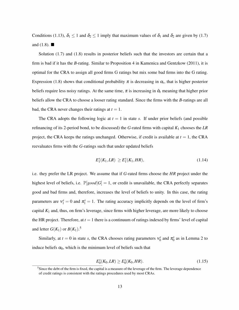
Solution (1.7) and (1.8) results in posterior beliefs such that the investors are certain that a

firm is bad if it has the B-rating. Similar to Proposition 4 in Kamenica and Gentzkow (2011), it is

optimal for the CRA to assign all good firms G ratings but mix some bad firms into the G rating.

Expression (1.8) shows that conditional probability p is decreasing in at , that is higher posterior

beliefs require less noisy ratings. At the same time, p is increasing in at meaning that higher prior

beliefs allow the CRA to choose a looser rating standard. Since the firms with the B-ratings are all

bad, the CRA never changes their ratings at t = 1.

The CRA adopts the following logic at t = 1 in state s. If under prior beliefs (and possible

refinancing of its 2-period bond, to be discussed) the G-rated firms with capital K1 chooses the LR

project, the CRA keeps the ratings unchanged. Otherwise, if credit is available at t = 1, the CRA

reevaluates firms with the G-ratings such that under updated beliefs

Es1(K1,LR) � Es

1(K1,HR), (1.14)

i.e. they prefer the LR project. We assume that if G-rated firms choose the HR project under the

highest level of beliefs, i.e. P[good|G] = 1, or credit is unavailable, the CRA perfectly separates

good and bad firms and, therefore, increases the level of beliefs to unity. In this case, the rating

parameters are ns1 = 0 and ps

1 = 1. The rating accuracy implicitly depends on the level of firm’s

capital K1 and, thus, on firm’s leverage, since firms with higher leverage, are more likely to choose

the HR project. Therefore, at t = 1 there is a continuum of ratings indexed by firms’ level of capital

and letter G(K1) or B(K1).5

Similarly, at t = 0 in state s, the CRA chooses rating parameters ns0 and ps

0 as in Lemma 2 to

induce beliefs a0, which is the minimum level of beliefs such that

Es0(K0,LR)� Es

0(K0,HR). (1.15)5Since the debt of the firm is fixed, the capital is a measure of the leverage of the firm. The leverage dependenceof credit ratings is consistent with the ratings procedures used by most CRAs.

13

Debt value: Due to limited liability if at maturity the value of firm’s capital is less than the face

value of the bond, the value of the debt is the value of capital less bankruptcy costs. Therefore, at

t = 2 the value of a bond belonging to a firm with capital K2 is

D2(K2) =

8

>

>

<

>

>

:

F if F K2

(1�d )K2 if F > K2,

(1.16)

where F is the bond’s face value. The following lemma gives the value of a bond at t = 1 in state

s if investors know which project is going to be chosen.

Lemma 3 Suppose a good firm with capital K1 chooses project p at t = 1. Then, its value at t = 1

is

Ds1(K1, p) = Â

s02Sl Q

ss0

h

(1�d )K1 eµs0p +0.5(s s0

p )2N(ds0

p ) + F N(�ds0p �s s0

p )i

, (1.17)

where dsp is defined in the statement of Lemma 1.

Proof The value of the debt is the expected value of repayment, i.e.

D1(K1) = Âs02S

l Qss0

Z •

0D2(rK1) f (r|µs0

p ,s s0p )dr, (1.18)

where f (r|µ,s) is the PDF of the log normal distribution with parameters µ and s . Since

D2(K2) =

8

>

>

<

>

>

:

F02, if K2 � F02

(1�d )K2, if K2 < F02,

(1.19)

the expected repayment can be written as

D1(K1) = Âs02S

l Qss0

h

Z F02/K1

0(1�d )rK1 f (r|µs0

p ,s s0p )dr+

Z •

F02/K1F02 f (r|µs0

p ,s s0p )dr

i

= Âs02S

l Qss0

h

(1�d )K1E⇥

r|r F02/K1,µs0p ,s s0

p⇤

P⇥

r F02/K1|µs0p ,s s0

p⇤

+F02P⇥

r > F02/K1|µs0p ,s s0

p⇤

i

, (1.20)

14

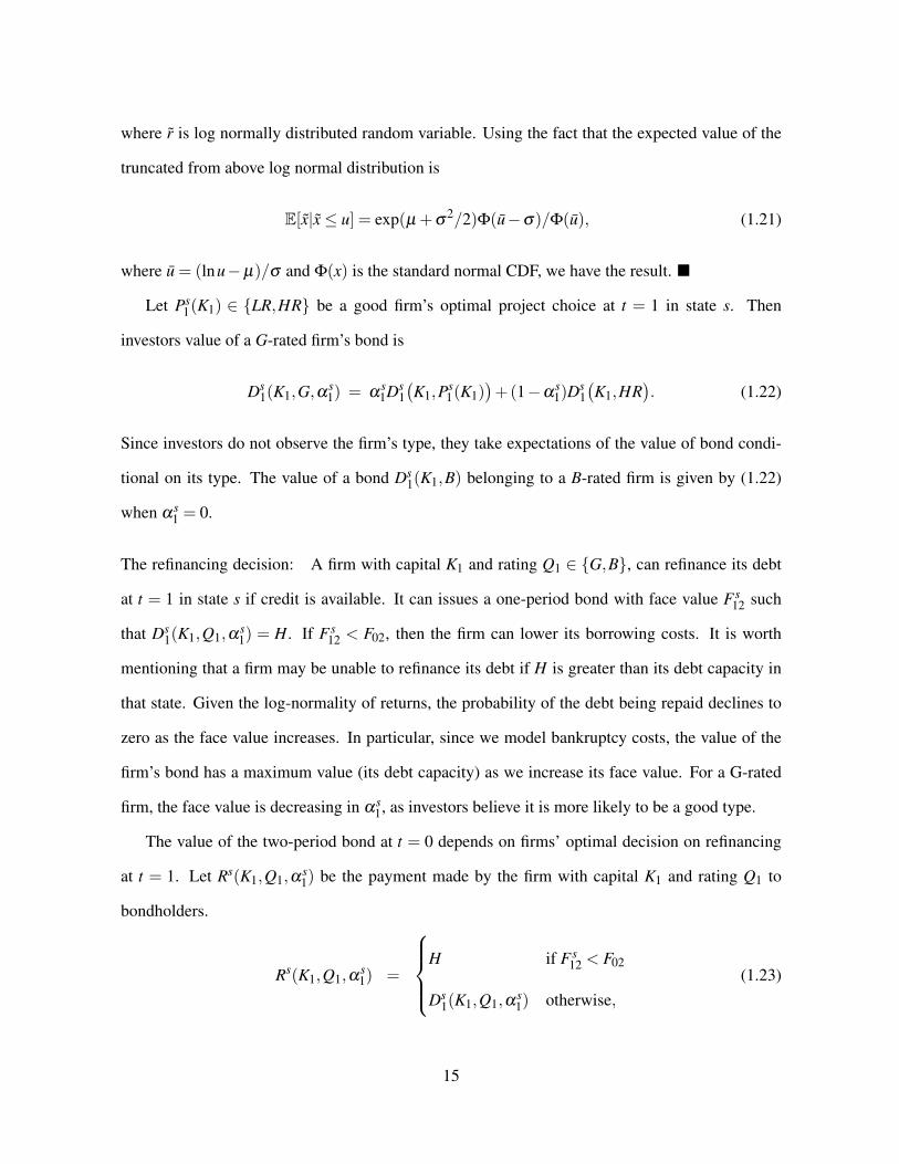
where r is log normally distributed random variable. Using the fact that the expected value of the

truncated from above log normal distribution is

E[x|x u] = exp(µ +s2/2)F(u�s)/F(u), (1.21)

where u = (lnu�µ)/s and F(x) is the standard normal CDF, we have the result. ⌅

Let Ps1(K1) 2 {LR,HR} be a good firm’s optimal project choice at t = 1 in state s. Then

investors value of a G-rated firm’s bond is

Ds1(K1,G,as

1) = as1Ds

1�

K1,Ps1(K1)

�

+(1�as1)D

s1�

K1,HR�

. (1.22)

Since investors do not observe the firm’s type, they take expectations of the value of bond condi-

tional on its type. The value of a bond Ds1(K1,B) belonging to a B-rated firm is given by (1.22)

when as1 = 0.

The refinancing decision: A firm with capital K1 and rating Q1 2 {G,B}, can refinance its debt

at t = 1 in state s if credit is available. It can issues a one-period bond with face value Fs12 such

that Ds1(K1,Q1,as

1) = H. If Fs12 < F02, then the firm can lower its borrowing costs. It is worth

mentioning that a firm may be unable to refinance its debt if H is greater than its debt capacity in

that state. Given the log-normality of returns, the probability of the debt being repaid declines to

zero as the face value increases. In particular, since we model bankruptcy costs, the value of the

firm’s bond has a maximum value (its debt capacity) as we increase its face value. For a G-rated

firm, the face value is decreasing in as1, as investors believe it is more likely to be a good type.

The value of the two-period bond at t = 0 depends on firms’ optimal decision on refinancing

at t = 1. Let Rs(K1,Q1,as1) be the payment made by the firm with capital K1 and rating Q1 to

bondholders.

Rs(K1,Q1,as1) =

8

>

>

<

>

>

:

H if Fs12 < F02

Ds1(K1,Q1,as

1) otherwise,(1.23)

15

Then if Ps0 2 {LR,HR} is the firm’s optimal project choice at t = 0 in state s, the value of the

two-period bond at t = 0 in state s is

Ds0(K0) = Â

s02Sl Q

ss0

⇣

as0 Eh

Rs0�r1K0,G,as1�

| Ps0 ,s

0i

(1.24)

+(1�as0) E

h

ps01�

r1K0�

Rs0�r1K0,G,as1�

| HR,s0i

+(1�as0) E

h

�

1�ps01�

r1K0��

Rs0�r1K0,B,0�

| HR,s0i⌘

,

where ps01�

K1�

is the probability that a bad firm with capital K1 retains the G-rating at t = 1 in state

s0. The first expectation in (1.24) corresponds to the value of the two-period bond of a good firm.

A bad firm rated G at t = 0 gets either G or B rating at t = 1. The bond of a bad firm that retains

the G-rating at t = 1 has the same value as the bond of a good firm. The bond of a bad firm that

gets downgraded at t = 1 has the value when investors are certain that the firm is bad. The second

and third expectations in (1.24) provide the values for these two mutually exclusive events.

1.3.1 Belief Updating From Learning and Bayesian Persuasion

At t = 0 all good firms start with the same level of capital and debt, and hence choose the same

project. At t = 1, updated beliefs of firms rated G being good, depend on the project return as

shown in (1.3). Figure 1.3 shows the level of beliefs, P(good|G), before and after observing ratings

at t = 1. As can be seen, the posterior of the firm being good, increases in the level of capital upto

a range, since the mean return of the LR project exceeds that of the HR project. For higher levels

of capital, the belief falls, as the relative likelihood of very high returns (capital) increase for the

HR project, which has a higher variance.

If K1 is sufficiently low (leverage of the firm is high), the asset substitution problem urges the

firm to choose the HR project. In particular, if K1 < K1, the firm chooses the HR project even

if investors are certain that the firm is good, i.e. P[good—G]=1, and the firm is able to refinance

its debt. In this case, we assume that the CRA chooses perfectly precise ratings and therefore

posterior beliefs, as1 ⌘ P[good|G] = 1. On the contrary, if the level of capital is sufficiently high,

i.e. K1 � K1, the firm chooses the LR project under any level of as1. In this case, the CRA does

16

not adjust the ratings and as1 = as

1. Finally, if K1 2 [K1,K1] (the shaded are in the figure), the

CRA is able to influence firms’ project choice at t = 1. With beliefs updated only after observing

project returns, as1, the firm chooses the HR project. In this case, the CRA increases the precision

of ratings such that under updated beliefs, as1, the G-rated firms would choose the LR project if

they could refinance their debt to lower their cost of capital. If credit is unavailable however, the

firms would continue to choose HR projects Therefore, the lack of credit is an additional factor of

systematic risk that coupled with a business downturn leads to the simultaneous increase of firms

risk. We use this mechanism to explain the dynamics of spreads on the tranches of a collateralized

debt obligation.

1.4 Securitized Debt

In this section we apply the model to price the tranches of a collateralized debt obligation (CDO).

The pricing of the tranches of a synthetic CDO with a large homogeneous collateral pool is similar

to that in Coval et al. (2009a) and Gibson (2005). We assume that at t = 0, the collateral pool

consists of a large number of callable two-period bonds issued by G-rated firms, each with capital

K0. The project choices by these firms at t = 0, and the realized returns on these projects implies

that at t = 1 their capital stocks differ, as do their leverage ratios. Moreover, the rating precision at

t = 1 depends on firms’ capital, contributing to an additional dispersion in investors’ beliefs about

these firms. As before, firms’ project returns bear purely idiosyncratic risk conditional on the state

of the economy. At t = 1 if credit is available the firms decide whether to refinance their debt. If a

firm refinances its bond, the newly issued bond replaces the old bond in the pool. Then the firms

again choose a project and end up with capital K2 at t = 2.

Since at t = 1 the pool is heterogeneous we cannot obtain the distribution of losses in a pool at

t = 2 in closed form as in Gibson (2005). Instead, to estimate the losses and determine the tranche

spreads at t = 1 we resort to a simulation technique. First, we simulate the levels of capital of

each firm in the pool at t = 1. In doing so, we fix state s at t = 0 and form a pool of N firms

17

with capital K0 and randomly assigned type such that probability of the good type is a0. For each

firm in the pool randomly determine the level of capital at t = 1 according to equation Ki1 = K0ri,

where random return ri is drawn from the log-normal distributions with parameters (µsP, s s

P) with

P project choice of the good firms at t = 0 and s state at t = 1 for a good firm and (µsHR, s s

HR) for

a bad firm.

Second, for each state s at t = 1 simulate the distribution of losses in the pool and calculate

average losses L[AL,AU ] on each CDO tranche with attachment points AL and AU . In particular,

we conduct T Monte-Carlo simulations and in each trial:

1. Given state s at t = 1 and transition probabilities l Qss0 randomly choose state s0 at

t = 2.

2. For each firm in the pool randomly determine the level of capital at t = 2 according

to equation Ki2 = Ki

1ri, where random return ri is drawn from the log-normal distri-

butions with parameters (µs0P , s s0

P ) with P project choice of the good firms at t = 1

and s0 state at t = 2 for a good firm and (µs0HR, s s0

HR) for a bad firm.

3. Calculate the value Di2(K2) of ith bond according to (1.16) and the total payoff of

the portfolio of N bonds

D⇤2 =

ÂNi=1 Di

2(K2)

ÂNi=1 Fi

⇤2,

where Fi⇤2 is equal Fi

02 if the ith bond has not been refinanced or Fi12 otherwise.

4. Calculate expected loss on each tranche with lower and upper attachment points AL

and AU

L[AL,AU ] = max(L⇤2 �AL,0)�max(L⇤

2 �AU ,0),

where L⇤2 = 1�D⇤

2.

Finally, given states at t = 0 and t = 1 we use the average losses on each tranche to calculate

18

the spreads for each tranche using equation

Sss[AL,AU ] =AU �AL

AU �AL � L[AL,AU ]�1.

1.5 Empirical Analysis

In this section, we structurally estimate our model and evaluate its implications for the pricing of

CDO tranches. Our empirical estimation is implemented in two stages. At the first stage we use

standard maximum likelihood of regime switching models (see Hamilton (1994)) to estimate the

cycles in credit availability and macroeconomic growth. The regimes are observed by the agents in

the model, but are unobserved by the econometrician. In the second stage, we use the simulation

method of moments (SMM) to estimate the parameters of firms’ projects that fit tranche spreads.

1.5.1 First Stage Maximum Likelihood Estimation of Regime Switching Model

The specification of the regime model is at the beginning of Section 1.2. Macro cycles are identified

as regimes of real GDP growth (states B and R), while credit cycles are identified as regimes in the

ratio of credit growth at nonfinancial companies to nominal GDP (A and N). We then form the four

composite states (BA), (R,A), (BN), and (R,N). The specification has homoskedastic fundamentals,

so that the volatility of each process is the same in each regime. We maximize the likelihood of

the econometrician observing these four composite regimes. It is useful to note, that we estimate

the model from 1951 to 2004, before the start of the CDO tranche data. Using these estimates, we

filter the data to provide the econometrician’s filtered probability of the underlying states in-sample

(1951 – 2004:Q2) and then out-of-sample (2004:Q3 – 2014). By doing so, we attempt to mitigate

over-fitting of tranche spreads in the second subsample. The time series of the ecoometrician’s

filtered probabilities are denoted as {wmc(t)}.

Parameter estimates of the model are in Table 1.2. As seen in the top panel, the ratio of credit

growth to GDP is about 2.5 times as high in A states relative to N states, although even the latter is

positive. This is consistent with our model in which firms can obtain credit with some probability

19

even in N states. Real GDP growth is about 4.5 percent (at an annual rate) in B states, and shrinks

at nearly 1 percent in R states. GDP growth is significantly more volatile than credit growth. The

quarterly transition matrix (and its standard errors) under the objective measure are in the two

subsequent panels. We will discuss the risk-adjusted transition matrix (under the Q-measure) in

a subsequent subsection. As in several other estimates of growth regimes, booms are far more

persistent than recessions. In addition, booms are more persistent in credit availability states.

Indeed, the RN state is the least persistent.

The econometrician’s filtered probabilities of the four composite regimes are in Figure 1.4. As

seen, each of the four regime probabilities become quite likely in different stages of the cycles.

Quite notably, the probabilities of BA regimes increase significantly in the middle of most NBER

recessions (shaded areas) in the sample. However, the probabilities of N (credit unavailability)

regimes, remain quite high even after the end of recessions. Therefore, credit availability lags

GDP growth, and a simple linear regression of credit growth on lagged GDP growth verifies this

intuition.

Ratio of Credit Growth(t)/GDP(t) = 0.219+0.451GDP Growth(t �4)+ e(t) (1.25)

[1.431] [3.306] (1.26)

where t-stats adjusted for autocorrelation and heteroskedasticity are in parenthesis.

Figure 1.5 shows that the expected growth rates from the model, fit the data quite well. In fact,

the regression of each of the realized data series on its expected value calculated using the regime

parameters and the filtered probabilities explains close to 57 percent of the variation in each series.

The plots also show that expected GDP growth troughs in recessions, while expected credit growth

troughs 2 to 4 quarters after the end of each recession. This was specially true for the last three

recessions.

While we have a reduced form specification of macro and credit regimes, our estimates are

consistent with the view that credit availability shrinks at the onset of weak growth, and persists

for several quarters even after growth resumes, perhaps because lenders become more cautious.

20

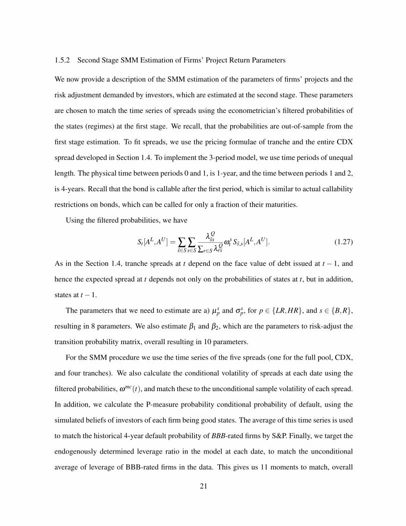
1.5.2 Second Stage SMM Estimation of Firms’ Project Return Parameters

We now provide a description of the SMM estimation of the parameters of firms’ projects and the

risk adjustment demanded by investors, which are estimated at the second stage. These parameters

are chosen to match the time series of spreads using the econometrician’s filtered probabilities of

the states (regimes) at the first stage. We recall, that the probabilities are out-of-sample from the

first stage estimation. To fit spreads, we use the pricing formulae of tranche and the entire CDX

spread developed in Section 1.4. To implement the 3-period model, we use time periods of unequal

length. The physical time between periods 0 and 1, is 1-year, and the time between periods 1 and 2,

is 4-years. Recall that the bond is callable after the first period, which is similar to actual callability

restrictions on bonds, which can be called for only a fraction of their maturities.

Using the filtered probabilities, we have

St [AL,AU ] = Âs2S

Âs2S

l Qss

Âr2S l Qrs

wst Ss,s[AL,AU ]. (1.27)

As in the Section 1.4, tranche spreads at t depend on the face value of debt issued at t � 1, and

hence the expected spread at t depends not only on the probabilities of states at t, but in addition,

states at t �1.

The parameters that we need to estimate are a) µsp and s s

p, for p 2 {LR,HR}, and s 2 {B,R},

resulting in 8 parameters. We also estimate b1 and b2, which are the parameters to risk-adjust the

transition probability matrix, overall resulting in 10 parameters.

For the SMM procedure we use the time series of the five spreads (one for the full pool, CDX,

and four tranches). We also calculate the conditional volatility of spreads at each date using the

filtered probabilities, wmc(t), and match these to the unconditional sample volatility of each spread.

In addition, we calculate the P-measure probability conditional probability of default, using the

simulated beliefs of investors of each firm being good states. The average of this time series is used

to match the historical 4-year default probability of BBB-rated firms by S&P. Finally, we target the

endogenously determined leverage ratio in the model at each date, to match the unconditional

average of leverage of BBB-rated firms in the data. This gives us 11 moments to match, overall

21

leading to an overidentified identified SMM estimator.

The parameter estimates are given in Table 1.3. As seen, both type of projects are riskier in

recession states. In addition, HR projects have higher risk and lower returns than LR projects in

each state.

1.5.3 Risk-Adjustment Parameters

The signs of the risk-adjustment for the growth and credit growth transitions in Table 1.3 are

quite compelling. As in common parlance, the price of risk of a shock is positive (negative) if it

over (under) weights the transition probability from a good to a bad state for investors. For our

estimated parameters, we find b1, the adjustment for the growth transition probability is positive,

as is consistent with several other empirical studies. Quite interestingly, our estimate of b2, the

credit growth transition, is negative. Above, we showed that credit growth remains strong at the

start of a recession, but then weakens, and remains weak after the end of the recession. Therefore,

credit growth shocks have a slightly countercyclical property, and hence has a negative price of

risk. The overall risk-adjustment across the composite states in our model does deliver us the

increase in credit spreads, which measure expected default losses under the Q-measure, to match

the historical spread level.

1.5.4 The Credit Spreads Puzzle, Spread Dynamics, and the Convexity Effect

Using the parameters estimated from the SMM procedure, we calculated the spreads for each of

the tranches in period t = 1 of the model for each state at t = 0. The state at t = 0 is relevant for the

spreads at t = 1, since it determines the proportion of firms choosing HR projects, and hence the

face values of debt. These implied spreads are in Table 1.4. As seen senior spreads S(15,100) are

zero in credit availability (A) states, while equity tranche spreads are close to their values in credit

unavailability (N) states. In the model, during N states, several firms cannot refinance their existing

debt, and hence, they choose HR projects. Therefore an increase in risk of some firms (relative to

A states) implies that the chance of the equity tranches experiencing significant losses increases.

22

But, since all firms do not increase their risk, the chance of all of them defaulting, an event that

triggers losses in the senior tranche, does not increase. Instead, the spreads for senior tranches, are

higher in low growth (R) states, where all firms’ volatility increases. This differential impact on

senior and junior tranches helps our model match the different dynamics of these tranches.

Using these state-dependent spreads, we calculate the fitted spreads at each date, which are

shown in Figure 1.6. Due to high risk-adjusted transition probabilities, the model is able to pro-

vide average spread levels fairly close to their historical averages, even as we match the objective-

measure average default probability. As in the credit spreads puzzle literature, this happens, be-

cause more defaults happen in recessions, which have boosted transition probabilities under the Q-

measure. In particular, the model’s spreads rose close to their historical values for junior tranches

in the great recession, but fell a bit short for senior tranches. Also, significantly, the model’s senior

tranche spreads, fell once economic growth picked up at the end of the recession, but the equity

tranche in particular remained at high levels until nearly 2010, when credit growth resumed. This

is in line with our motivating regressions in the introduction, where a much larger proportion of

the equity tranche is explained by credit growth rather than economic growth, while the reverse is

true for the senior tranche. Overall, the model-fitted spreads explain between 51 percent (equity

tranche S(0,3)) and 71 percent (S(15,100) tranche), with better for senior tranches.

One of the key aspects of our model is the endogenously generated convexity effect of credit

spreads. As was pointed out by David (2008), essentially in structural form models of credit

risk (such as this one), credit spreads are convex function of firms’ asset values (capital stocks).

Due to heterogeneity in firms’ capital accumulation, spreads for firms with low realized capital

rise more dramatically, then for the fall of spreads of firms that have high realized capital. The

greater the dispersion in capital stocks across firms, the greater is the difference in average spreads

across firms, and the spread calculated for a representative firm with an average capital stock. In

the model, heterogeneity increases in low growth states, but also to some extent when credit is

unavailable. Therefore spreads increase in such states. The convexity effect not only implies an

23

increase in the average spread generated by the model, but also the dynamics of spreads, as spreads

increases in states with higher dispersion, which endogenously varies as the economy transitions

through the macro and credit states. Figure 1.7 shows the distribution of firm’s capital stocks at

t=1 in four possible states of the economy.

As mentioned above, the convexity effect arises endogenously in our model. In particular, as

the CRA changes the precision of its rating over time, it affects the dispersion in borrowing costs

across firms, which in turn affects their project choices, and the dispersion in their capital stocks.

This is a feature not present in prior work on the convexity effect, such as in David (2008).

1.6 Data Description

We obtain monthly time series of tranche spreads on synthetic CDOs based on the DJ CDX North

American Investment Grade Index (CDX.NA.IG). This index consists of an equally weighted port-

folio of 125 credit default swap (CDS) contracts on US firms with investment grade debt. Our sam-

ple covers the eleven year period from September 2004 to October 2014. The data from September

2007 to October 2014 is provided by Bloomberg (CMA New York). The data from September 2004

to August 2007 is from Coval et al. (2009a).

The CDX indices roll every six months. In particular, on September 20 and March 20 new

series of the index with updated constituents are introduced. After a new series is created, the

previous series continue trading though liquidity is usually concentrated on the on-the-run series.

An exception is series 9 introduced in September 2007 and traded till the end of 2012 together

with less liquid on-the-run series. The CDX indices have 3, 5, 7 and 10 year tenors. We use 5 year

CDX indices which are most liquid for most series.

We build our sample from on-the-run series except period from March 2008 to September 2010

where we use most liquid series 9. Before series 15 introduced in September 2010 the CDX index

has been traded with tranches 0-3%, 3-7%, 7-10%, 10-15%, 15-30% and 30-100%.6 Starting from6The tickers of the tranches of series 9 are CT753589 Curncy, CT753593 Curncy, CT753597 Curncy, CT753601

24

series 15 and onward, only odd series of the index are traded with tranches and the structure of

tranches changes to 0-3%, 3-7%, 7-15% and 15-100%.7

We focus our analysis on the equity and the most senior tranches. Since the equity 0-3%

tranche is quoted as an upfront payment, we calculate the par spread using the formula S0�3% =

500b.p.+U/D where U is the upfront fees and D is the time to maturity of the tranche. While

earlier series (before 15) have tranches 15-30% and 30-100%, there is only one tranche 15-100%

for later series. To make the series consistent we create a tranche 15-100% for earlier series as the

sum of tranches 15-30% and 30-100%.

We obtain credit growth at nonfinancial corporate businesses from the Federal Reserve Board’s

flow of funds accounts (series FA104104005.Q), and nominal and real GDP from the St. Louis

Fed FRED database.

1.7 Conclusion

In this paper, we provide a new model to show how imperfect credit ratings and occurrence of

credit crunches can create catastrophic risk observed in the prices of CDO tranches. There are

three crucial ingredients in our model. First, we endogenize firms’ risk-taking using the asset

substitution mechanism. In particular, the firms choose the riskiness of their projects based on the

amount of debt that they need to service. Second, a credit rating agency changes the intensity of the

investigation of firms’ credit quality to maximize the proportion of firms with high credit ratings.

Finally, the credit shortage can trigger firms’ risky behaviour if they are unable to refinance their

debt under a more precise rating standard. This increases the risk of senior tranches of structured

finance products.

We structurally estimate the parameters of our dynamic Bayesian persuasion model and show

Curncy, CT753605 Curncy, CT753609 Curncy.7The tickers of the tranches of series 15, 17, 19 and 21 are CY071225 Curncy, CY071229 Curncy, CY071233

Curncy, CY071237 Curncy, CY087579 Curncy, CY087583 Curncy, CY087587 Curncy, CY087591 Curncy,CY125375 Curncy, CY125380 Curncy, CY125385 Curncy, CY125390 Curncy, CY181667 Curncy, CY181672Curncy, CY181677 Curncy and CY181682 Curncy.

25

that it can shed light on the puzzling phenomenon that senior tranche spreads are relatively more

exposed to growth shocks, while junior spreads are more exposed to credit availability shocks.

In particular, refinancing of existing debt may not be possible during a credit crunch, and hence

the resulting high risk strategy for some firms in such periods implies that junior tranches, get

seriously impacted. In contrast senior tranches get affected by growth shocks, which increase

the risk of all firms’ projects. A crucial aspect of our model is that an endogenously generated

“convexity effect”, in large part due to the time varying precision of credit ratings, is much more

important in understanding CDO tranche spreads than the spread on the entire pool of firms, the

subject of past studies.

26

Table 1.1: What Explains CDO Tranche Spreads?

No. a b1 b2 R2

CDX Spread1. 111.61 -49.31 0.433

[8.71] [-3.88]2. 113.69 -51.57 0.344

[7.30] [-3.08]3. 126.84 -43.036 -42.89 0.669

[14.29] [-4.96] [-6.31]Spread (0-3)4. 1564.69 10.73 0.145

[10.73] [-2.50]5. 1717.56 -646.36 0.508

[15.11] [-4.73]6. 1779.44 -205.87 -604.85 0.577

[17.01] [-3.58] [-4.42]Spread (3-7)7. 627.11 -362.28 0.362

[5.48] [-3.04]8. 686.00 -484.66 0.470

[114.18] [126.75]9. 777.69 -300.23 -424.13 0.711

[10.30] [-4.22] [-7.76]Spread (7-15)10. 406.83 -343.59 0.498

[4.53] [-3.32]11. 410.68 -333.43 0.341

[3.57] [-2.60]12. 503.47 -303.78 -272.17 0.718

[6.898] [-4.17] [-5.49]Spread (15-100)13. 66.67 -53.30 0.564

[6.06] [-4.88]14. 60.48 -35.26 0.179

[3.53] [-1.94]15. 75.64 -49.61 -25.26 0.653

[-5.28] [-3.17]Tranche spreads are on the Dow Jones North American Investment Grade Index, which are reported by CreditMarket Analysis (CMA) and obtained from Bloomberg (see Data Appendix for construction of our time series).CDX represents the full CDO. Spread (AL,AU) represents the spread on a trance with loss attachment points ALand AU in percentage points. For example, the “senior” spread represents the 15 to 100 percent loss attachmentpoints, while the “equity” tranche represents the 0 to 3 loss attachment points. We report the coefficients of thefitted regression:

Tranche Spread(t) = a + b1 Real GDP Growth + b2 Credit Growth(t)/GDP(t)+ e(t)

for alternative tranches T-statistics are in parenthesis and are adjusted by White’s procedure for heteroskedasticity.

27

Table 1.2: Maximum Likelihood Estimates of 4-Regime Markov Switching Model for Ratio ofCredit Growth at Nonfinancial Firms to GDP and Real GDP Growth

Ratio of Credit Growth to GDP (%)µ1

c µ2c

0.901 0.366(0.185) (0.005)

Quarterly Real GDP Growth (%)µ1

g µ2g

1.109 -0.237(0.031) (0.002)

Volatilities (%)sg sc

0.251 0.755(7.432) (0.019)

Standard errors are in parenthesis.

Quarterly Transition Probability Matrix (Estimates)(BA) (RA) (BN) (RN)

(BA) 0.930 0.000 0.039 0.030(RA) 0.168 0.832 0.000 0.000(BN) 0.000 0.000 0.900 0.099(RN) 0.102 0.119 0.133 0.644

Quarterly Transition Probability Matrix (Asymptotic Standard Errors)(BA) (RA) (BN) (RN)

(BA) 3.624⇥10�04 1.338⇥10�4 1.363⇥10�04

(RA) 3.96⇥10�04 1.652⇥10�04 6.081⇥10�04

(BN) 8.322⇥10�04 3.713⇥10�04 2.199⇥10�04

(RN) 5.054⇥10�04 4.482⇥10�04 2.55⇥10�04

Log Likelihood =-401.725

28

Table 1.3: Second Stage SMM Estimation of Firms’ Project and Risk Adjustment Parameters

Firms’ Project ParametersµB

LR 0.132 sBLR 0.019

µRLR 0.047 sB

LR 0.035µB

HR 0.022 sBHR 0.036

µRHR 0.002 sR

HR 0.152

Risk Adjustment Parametersb1 0.129 b2 -0.220

J-Statistic = 0.988

Table 1.4: Implied Spreads (In Basis Points) From SMM Parameter Estimates

CDX S(0,3) S(3,7) S(7,15) S(15,100)

State at t=0 is (BA)(BA) 27 559 258 36 0(RA) 290 1344 1067 1067 173(BN) 37 1031 278 29 0(RN) 243 5729 873 574 119State at t=0 is (BN)(BA) 27 559 258 36 0(RA) 234 1067 1067 1067 116(BN) 37 1031 278 29 0(RN) 159 1422 574 574 74State at t=0 is (RA)(BA) 27 559 258 36 0(RA) 290 1344 1067 1067 173(BN) 37 1031 278 29 0(RN) 243 5729 873 574 119State at t=0 is (RN)(BA) 27 559 258 36 0(RA) 253 1104 1067 1067 136(BN) 37 1031 278 29 0(RN) 198 2529 627 574 99

29

Figure 1.1: Tranche Spreads, Economic Growth, and Credit Availability

0

40

80

120

160

200

04 05 06 07 08 09 10 11 12 13 14

CDO Senior Tranche: S(15,100)

Ba

sis

Po

ints

400

800

1,200

1,600

2,000

2,400

2,800

04 05 06 07 08 09 10 11 12 13 14

CDO Equity Tranche (0,3)

Ba

sis

Po

ints

-2.5

-2.0

-1.5

-1.0

-0.5

0.0

0.5

1.0

1.5

04 05 06 07 08 09 10 11 12 13 14

Quarterly Real GDP Growth

Pe

rce

nta

ge

Po

ints

-1.5

-1.0

-0.5

0.0

0.5

1.0

1.5

04 05 06 07 08 09 10 11 12 13 14

Ratio of Credit Growth at Nonfinancial Firms to GDP

Pe

rce

nta

ge

Po

ints

Tranche spreads are on the Dow Jones North American Investment Grade Index, which are reported by Credit MarketAnalysis (CMA) and obtained from Bloomberg (see Data Appendix for construction of our time series). The “senior”spread represents the 15 to 100 percent loss attachment points, while the “equity” tranche represents the 0 to 3 lossattachment points.

30

Figure 1.2: Sequence of Events

Good firms choose LR or HRand invests all its capital.

The firm issues a two-periodbond with face value F02 andcall price H.

If the credit is available, thefirm may refinance its debt, i.e.pay call price H and issue aone-period bond with face valueF12 to finance the repayment.

If refinanced at t = 1 thefirm repays F12; other-wise the firm repays F02.

t=2BA/BN/RA/RN

t=1BA/BN/RA/RN

t=0BA/RA

(RE-)RATING

FINANCING

INVESTMENT

The CRA produces ratings andmoves investors’ belief from ↵0

to ↵0.

Investors observe project out-come and update their beliefs to↵1. If necessary, the CRA ad-justs ratings so that investorsupdate their beliefs from ↵1 to↵1.

Good firms choose LR/HRand invests all its capital.

31

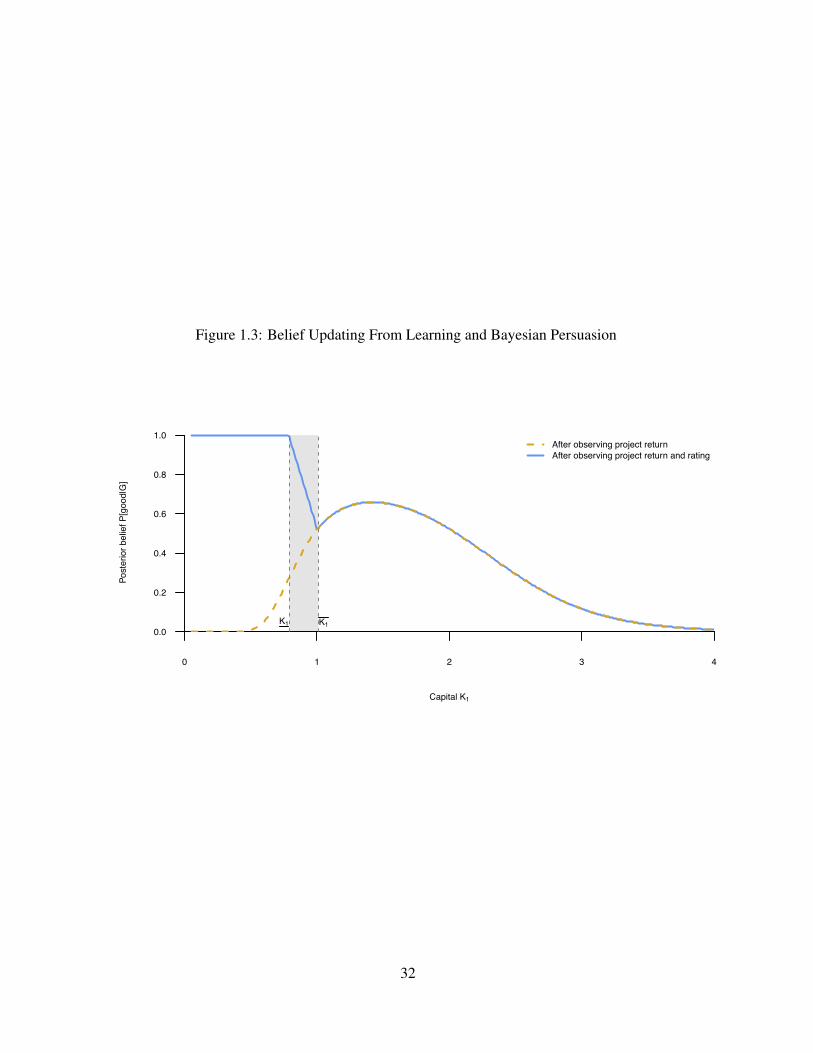
Figure 1.3: Belief Updating From Learning and Bayesian Persuasion

0 1 2 3 4

0.0

0.2

0.4

0.6

0.8

1.0

Capital K1

Post

erio

r bel

ief P

[goo

d|G

]

After observing project returnAfter observing project return and rating

K1 K1

32

Figure 1.4: Probabilities of the States From Regime Switching Model (1950:Q1 – 2014:Q4)

0.0

0.2

0.4

0.6

0.8

1.0

55 60 65 70 75 80 85 90 95 00 05 10

Probability of High Credit and High GDP Growth

0.0

0.2

0.4

0.6

0.8

1.0

55 60 65 70 75 80 85 90 95 00 05 10

Probability of High Credit and Low GDP Growth

0.0

0.2

0.4

0.6

0.8

1.0

55 60 65 70 75 80 85 90 95 00 05 10

Probability of Low Credit and High GDP Growth

0.0

0.2

0.4

0.6

0.8

1.0

55 60 65 70 75 80 85 90 95 00 05 10

Probability of Low Credit and Low GDP Growth

33

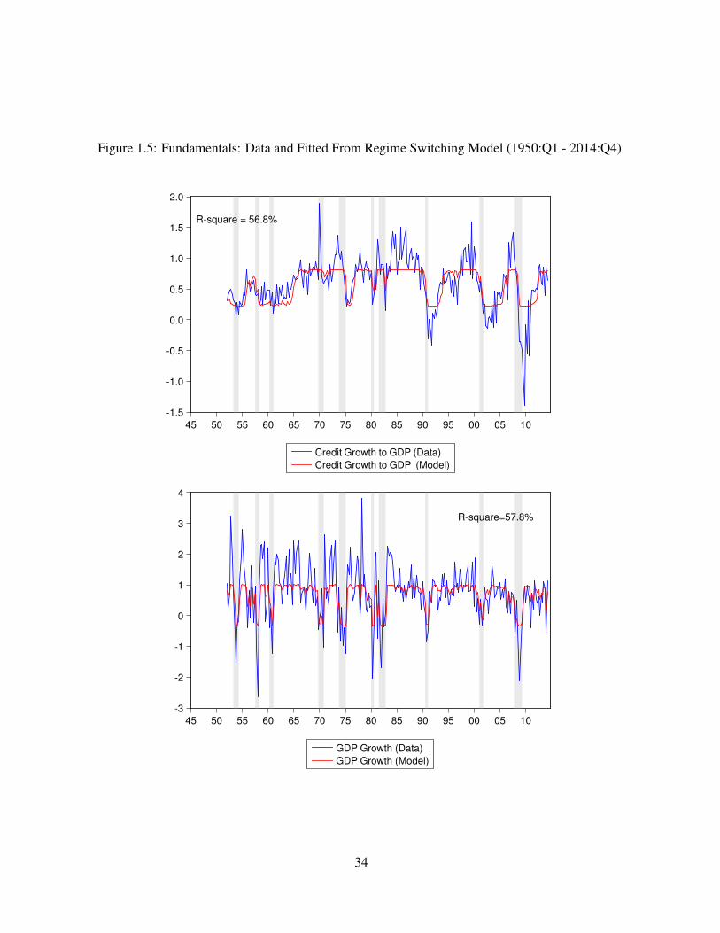
Figure 1.5: Fundamentals: Data and Fitted From Regime Switching Model (1950:Q1 - 2014:Q4)

-1.5

-1.0

-0.5

0.0

0.5

1.0

1.5

2.0

45 50 55 60 65 70 75 80 85 90 95 00 05 10

Credit Growth to GDP (Data)Credit Growth to GDP (Model)

-3

-2

-1

0

1

2

3

4

45 50 55 60 65 70 75 80 85 90 95 00 05 10

GDP Growth (Data)GDP Growth (Model)

R-square = 56.8%

R-square=57.8%

34

Figure 1.6: Model and Actual Spreads on Senior and Equity Tranches

R2 = 0.603

50

100

150

200

2006 2008 2010 2012 2014

Actual

Model

CDX

R2 = 0.514

1000

1500

2000

2500

2006 2008 2010 2012 2014

Actual

Model

0−3% Tranche

R2 = 0.601

500

1000

1500

2006 2008 2010 2012 2014

Actual

Model

3−7% Tranche

R2 = 0.602

500

1000

2006 2008 2010 2012 2014

Actual

Model

7−15% Tranche

R2 = 0.712

50

100

150

2006 2008 2010 2012 2014

Actual

Model

15−100% Tranche

35

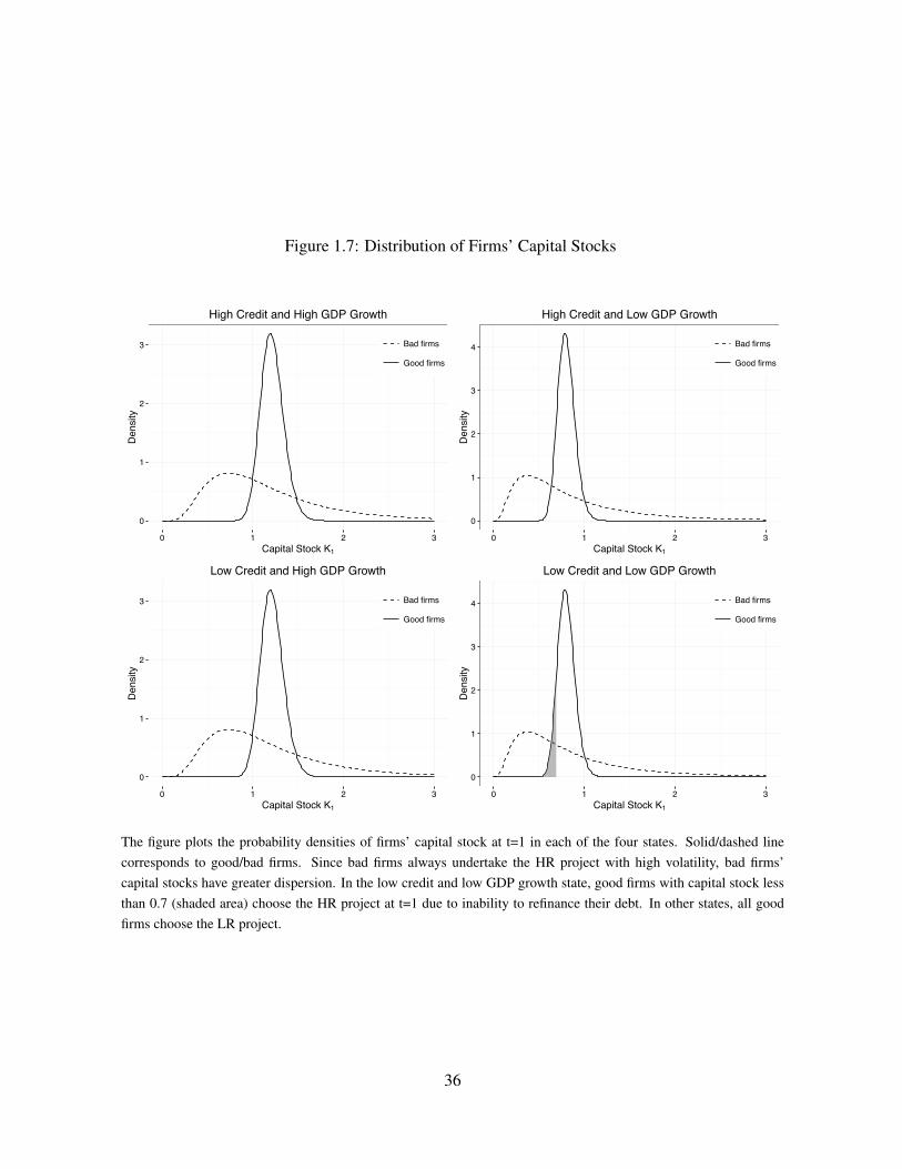
Figure 1.7: Distribution of Firms’ Capital Stocks

0

1

2

3

0 1 2 3Capital Stock K1

Den

sity

Bad firms

Good firms

High Credit and High GDP Growth

0

1

2

3

0 1 2 3Capital Stock K1

Den

sity

Bad firms

Good firms

Low Credit and High GDP Growth

0

1

2

3

4

0 1 2 3Capital Stock K1

Den

sity

Bad firms

Good firms

High Credit and Low GDP Growth

0

1

2

3

4

0 1 2 3Capital Stock K1

Den

sity

Bad firms

Good firms

Low Credit and Low GDP Growth

The figure plots the probability densities of firms’ capital stock at t=1 in each of the four states. Solid/dashed linecorresponds to good/bad firms. Since bad firms always undertake the HR project with high volatility, bad firms’capital stocks have greater dispersion. In the low credit and low GDP growth state, good firms with capital stock lessthan 0.7 (shaded area) choose the HR project at t=1 due to inability to refinance their debt. In other states, all goodfirms choose the LR project.

36

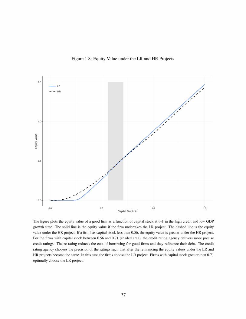
Figure 1.8: Equity Value under the LR and HR Projects

0.0

0.5

1.0

1.5

0.0 0.5 1.0 1.5Capital Stock K1

Equi

ty V

alue

LR

HR

The figure plots the equity value of a good firm as a function of capital stock at t=1 in the high credit and low GDPgrowth state. The solid line is the equity value if the firm undertakes the LR project. The dashed line is the equityvalue under the HR project. If a firm has capital stock less than 0.56, the equity value is greater under the HR project.For the firms with capital stock between 0.56 and 0.71 (shaded area), the credit rating agency delivers more precisecredit ratings. The re-rating reduces the cost of borrowing for good firms and they refinance their debt. The creditrating agency chooses the precision of the ratings such that after the refinancing the equity values under the LR andHR projects become the same. In this case the firms choose the LR project. Firms with capital stock greater than 0.71optimally choose the LR project.

37

Bibliography

Bar-Isaac, H. and Shapiro, J. (2011), ‘Credit ratings accuracy and analyst incentives’, American

Economic Review 101, 120–24.

Bhamra, H., Kuehn, L.-A. and Strebulaev, I. (2009), ‘The levered equity risk premium and credit

spreads: A unified framework’, Review of Financial Studies 23, 645–703.

Bolton, P., Freixas, X. and Shapiro, J. (2012), ‘The credit ratings game’, Journal of Finance

67(1), 85 – 111.

Boot, A. W. A., Milbourn, T. T. and Schmeits, A. (2006), ‘Credit ratings as coordination mecha-

nisms.’, Review of Financial Studies 19(1), 81 – 118.

Chen, H. (2010), ‘Macroeconomic conditions and the puzzles of credits spreads and capital struc-

ture’, Journal of Finance 65, 2171–2212.

Chen, H., Cui, R., He, Z. and Milbrandt, K. (2015), Quantifying liquidity and default risks of cor-

porate bonds over the business cycle. Working Paper, University of Chicago, Booth School

of Business.

Chen, L., Collin-Dufresne, P. and Goldstein, R. S. (2009), ‘On the relation between credit spread

puzzles and the equity premium puzzle’, Review of Financial Studies 22, 3367–3409.

Christoffersen, P., Du, D. and Elkamhi, R. (2013), Rare disasters and credit market puzzles. Work-

ing Paper, University of Toronto, Rotman School of Business.

Cohn, J. B., Rajan, U. and Strobl, G. (2013), Credit ratings: Strategic issuer disclosure and optimal

screening. Available at SSRN: http://ssrn.com/abstract=2360334.

Collin-Dufresne, P., Goldstein, R. S. and Yang, F. (2012), ‘On the relative pricing of long-maturity

index options and collateralized debt obligations.’, Journal of Finance 67(6), 1983 – 2014.

38

Cooper, R. (1999), Coordination Games, Cambridge University Press.

Coval, J. D., Jurek, J. W. and Stafford, E. (2009a), ‘Economic catastrophe bonds.’, The American

Economic Review 99(3), 628.

Coval, J. D., Jurek, J. W. and Stafford, E. (2009b), ‘The economics of stuctured finance’, Journal

of Economic Perspectives 23(1), 3–25.

Culp, C. L., Nozawa, Y. and Veronesi, P. (2015), Option-based credit spreads. Working Paper

University of Chicago, Booth School of Business.

David, A. (2008), ‘Inflation uncertainty, asset valuations, and the credit spreads puzzle’, Review of

Financial Studies 21, 2487–2534.

Feldhutter, P. and Schaefer, S. (2015), The credit spread puzzle in the merton model — myth or

reality? Working Paper, London Business School.

Fulghieri, P., Strobl, G. and Xia, H. (2014), ‘The economics of solicited and unsolicited credit

ratings.’, Review of Financial Studies 27(2), 484 – 518.

Gibson, M. S. (2005), ‘Understanding the risk of synthetic cdos’, ICFAI Journal of Risk and In-

surance 2, 21–43.

Hamilton, J. D. (1994), Time Series Analysis, Princeton University Press, Princeton, New Jersey.

Harris, M., Opp, C. and Opp, M. (2013), ‘Rating agencies in the face of regulation’, Journal of

Financial Economics 108, 46–61.

Kamenica, E. and Gentzkow, M. (2011), ‘Bayesian persuasion.’, American Economic Review

101(6), 2590 – 2615.

Kartasheva, A. and Yilmaz, B. (2012), Precision of ratings. Available at SSRN:

http://ssrn.com/abstract=2232998.

39

Kuehn, L.-A. and Schmid, L. (2014), ‘Investment-based corporate bond pricing’, Journal of Fi-

nance 69, 2741 – 2776.

Lizzeri, A. (1999), ‘Information revelation and certification intermediaries’, Rand Journal of Eco-

nomics 30, 214–231.

Manso, G. (2013), ‘Feedback effects of credit ratings’, Journal of Financial Economics 109, 535–

548.

Milgrom, P. and Roberts, J. (1990), ‘Rationalizability, learning, and equilibrium in games with

strategic complementarities’, Econometrica 58(6), 1255–77.

Wojtowicz, M. (2014), ‘Cdos and the financial crisis: Credit ratings and fair premia’, Journal of

Banking and Finance 39(0), 1 – 13.

40

Chapter 2

User Costs, the Financial Firm, and Monetary

and Regulatory Policy

Joint paper with Apostolos Serletis

2.1 Introduction

The current mainstream approach to monetary policy and business cycle analysis is based on the

new Keynesian model and is expressed in terms of the interest rate on overnight loans between

banks, such as the federal funds rate in the United States. This approach ignores the financial

intermediary sector. As Adrian and Shin (2011, p. 602) put it, “in conventional models of mon-

etary economics commonly used in central banks, the banking sector has not played a prominent

role. The primary friction in such models is the price stickeness of goods and services. Finan-

cial intermediaries do not play a role, except as a passive player that the central bank uses as a

channel to implement monetary policy.” However, banks and other financial intermediaries have

been at the center of the global financial crisis, and there is almost universal agreement that the

crisis originated in the financial intermediary sector. There is also a number of recent theories that

give financial intermediaries a central role in economics and finance. See, for example, Fostel

and Geanakoplos (2008), Geanakoplos (2010), He and Krishnamurthy (2013), and Adrian et al.

(2014).

However, it is not uniform view in the literature as to what financial intermediaries do. As

Diewert et al. (2012) put it, “one of the most controversial areas in the field of economic mea-

surement is the measurement of the real and nominal output of the banking sector. There is little

consensus on all aspects of this topic: even the measurement of banking sector nominal outputs

41

and inputs is controversial and there is little agreement on how to measure the corresponding real

outputs and inputs.” There is also a broader aspect to what banks do than just being financial inter-

mediaries. Banks are allowed to create money and play an important role in the monetary policy

transmission process. In this regard, the current approach to monetary policy also ignores the role

of money, as the short-term nominal interest rate is the sole monetary variable and there is no

reference to any monetary aggregate.

In this paper we follow Hancock (1985) and take a microeconomic theory approach to the fi-

nancial firm in an attempt to elevate financial intermediaries to the center stage of business cycles

and economic growth. We assume that the banking firm is a profit-maximizing entity producing

intermediation services between lenders and borrowers. We take the user cost approach to the con-

struction of prices for monetary and nonmonetary goods. This approach to modelling the banking

firm has rarely been implemented in practice and permits monetary goods (such as cash and de-

posits of various types), other financial goods (such as loans), and physical goods (such as labor

and materials) to be classified as inputs or outputs. Those items with a positive user cost are

classified as inputs and those with a negative user cost are classified as outputs. More importantly,

the user cost approach explicitly takes into account each bank’s cost of funds, as user costs are

calculated based on each bank’s cost of capital. This makes decision problem comparable across

financial institutions. For example, the same investment opportunity could be profitable for a bank

with a low cost of capital but unprofitable for a bank with a high cost of capital. Thus, the optimal

demands for and supplies of monetary and nonmonetary goods vary across institutions, an aspect

of banking that is often ignored in the literature.

The technology of the financial firm is relevant in the investigation of the demand for and supply

of monetary and nonmonetary goods and their substitutability/complementarity relationship. It is

also relevant in the conduct of monetary policy and the investigation of the effects of financial

regulation. One approach to financial technology is to estimate cost functions in which input costs

and output quantities are the explanatory variables. In this approach to bank technology, however,

42

output is not a predetermined variable and it is difficult to distinguish between inputs and outputs.

In this paper we take an alternative (and more promising) approach based on the variable profit

function, which depends on prices of outputs and inputs and the quantities of fixed inputs.

In doing so, we also provide a comparison among three flexible functional forms for the

variable profit function — the translog, the symmetric generalized Barnett, and the Normalized

Quadratic (NQ), the latter also known in the literature as symmetric generalized McFadden. We

use recent, state-of-the-art advances in microeconometrics to produce inference consistent with

theoretical regularity — see, for example, Barnett and Serletis (2008) and Feng and Serletis (2008).

In particular, motivated by the wide-spread practice of ignoring theoretical regularity, we estimate

the translog, NQ, and symmetric generalized Barnett variable profit functions subject to the con-

vexity conditions and produce inference consistent with neoclassical microeconomic theory. Our

objective is to identify the channels through which financial intermediaries affect the real economy,

and investigate the implications for regulatory and monetary policies.

The paper is organized as follows. In Section 2, we provide a brief review of two fundamen-

tally different approaches to modeling the banking firm — the accounting balance-sheet approach

(or intermediation approach) of Sealey and Lindley (1977) and the user-cost approach. In Section

3 we discuss the variable profit function approach and in Section 4 we discuss the three flexible

functional forms for the variable profit function as well as the procedures for imposing convexity

on each of these functions in order to achieve theoretical regularity. In Section 5 we deal with

data issues. Our primary focus is on empirical application, specifically to annual data on the U.S.

commercial banking sector, over the period from 1992 to 2013, obtained from the quarterly Uni-

form Bank Performance Reports (UBPR) provided by the Federal Deposit Insurance Corporation.

Section 6 discusses related econometric issues and in Section 7 we estimate the models, present

the empirical results, and provide a comparison among the three flexible functional forms for the

variable profit function. In Section 8, we conduct a monetary and regulatory policy analysis. The

final section concludes the paper.

43

2.2 The User Cost Approach

A long-standing debate over the inputs and outputs of the banking technology has shaped sev-

eral approaches to modelling the banking firm. We briefly discuss two of them: the Sealey and

Lindley’s (1977) intermediation approach and the Barnett (1978) and Hancock (1985) user cost

approach. Although these two approaches have many implications in common, they stem from

conceptually different premises. The intermediation approach posits that, by nature, banks are fi-

nancial liaisons between liability holders and those who receive bank funds. This premise suggests

that all bank assets including loans and leases, investments in securities, and reserves are outputs

for the banking technology. At the same time, all bank liabilities such as deposits, other debt,

and equity capital are inputs. Sealey and Lindley (1977, p. 1253) claim that deposits, the most

controversial part of liabilities, are an economic input since “these services require the financial

firm to incur positive costs without yielding any direct revenue.” Classifying deposits as inputs

has exposed the intermediation approach to criticism for neglecting substantial services that banks

provide to their depositors. Later, the literature has attempted to disentangle the intermediation

and deposit services of banks. See Berger and Humphrey (1992) for discussion.

The user cost approach arises from an intertemporal model of the banking firm which chooses

the quantities of different assets and liabilities to maximize profit. This approach renounces the

ex-ante classification of assets and liabilities and instead derives the nature of the financial goods

based on their contribution to the bank profit. In particular, an asset is considered to be an output

if the return on investment into this asset exceeds the opportunity cost of funds. Similarly, a

liability is classified as an output if the financial cost of this liability is less than the opportunity

cost of funds. According to this classification scheme, deposits are likely to be labeled as outputs,

especially, if only interest expenses are taken into consideration. Interestingly, because of different

cost of funds, the same asset or liability can be classified as input in one bank and as output in

another. For this same reason, the nature of a financial good can change over time.

A formal representation of the user cost approach can be found in Barnett (1978, 1987), Barnett

44

and Hahm (1994), Barnett and Zhou (1994), Barnett et al. (1995), and Hancock (1985, 1991).

Here, we begin with Barnett’s (1978) definition of user costs and Hancock’s (1985) application of

the user cost approach to the banking firm. In doing so we construct user costs (per unit, with the

unit taken to be one dollar per period) for the services from all assets and liabilities in a financial

firm’s balance sheet. Following Hancock (1985), we model banks that maximize the capitalized

value of variable profit over a certain period of time. Since we estimate the model using annual

data, we assume that banks can fully adjust the quantities of the goods to optimal values every year.

The absence of adjustment costs effectively reduces our setup to a one-period profit maximization

problem.

We assume that there are N banks in the economy (indexed by i) and each bank operates with

n financial goods indexed by k. The first A financial goods, i.e. k = 1, ...,A, are assets and the

following L, i.e. k = A+ 1, ...,A+L are liabilities, so that n = A+L. We let Pt denote a general

price index in period t, ykit the real balance and hk

it the holding cost/revenue (per unit) of the kth

financial good of bank i in period t. Besides, we let yit to be the quantity of a fixed in the short run

good of bank i in period t. Then the variable profit of bank i during period t is

git =A

Âk=1

h⇣

1+hki,t�1

⌘

yki,t�1Pt�1 � yk

itPt

i

+A+L

Âk=A+1

h

ykitPt �

⇣

1+hki,t�1

⌘

yki,t�1Pt�1

i

. (2.1)

In equation (2.1), for a liability k (such as a deposit), ykitPt �

⇣

1+hki,t�1

⌘

yki,t�1Pt�1 represents

the total net cost of services to the firm and equals the total nominal liability to depositors at the

end of the period, ykitPt , minus the initial nominal liability, yk

i,t�1Pt�1, and holding costs or revenues

incurred at the rate hki,t�1, hk

i,t�1yLi,t�1Pt�1. For an asset k (such as a loan),

⇣

1+hki,t�1

⌘

yki,t�1Pt�1 �

ykitPt represents the total net revenue to the firm during period t and equals the initial nominal asset,

yki,t�1Pt�1, plus holding revenue incurred at the rate hk

i,t�1, hki,t�1yk

i,t�1Pt�1, minus the total nominal

asset at the end of the period, ykitPt .

If Ris is the ith bank discount rate in period s, then the capitalized value of variable profit over

45

T periods is

T

Ât=2

t

’s=1

1(1+Ris)

git =T

Ât=2

t

’s=1

1(1+Ris)

A

Âk=1

h⇣

1+hki,t�1

⌘

yki,t�1Pt�1 � yk

itPt

i

+T

Ât=2

t

’s=1

1(1+Ris)

A+L

Âk=A+1

h

ykitPt �

⇣

1+hki,t�1

⌘

yki,t�1Pt�1

i

. (2.2)

The negative of the coefficients of real balances, ykit , in equation (2.2) are beginning of the

period nominal user costs — see also Barnett (1978). Thus, the beginning of period nominal user

cost for assets is

ukit =

✓

Rit �hkit

1+Rit

◆

Pt , k = 1, ...,A (2.3)

and that for liabilities is

ukit =

✓

hkit �Rit

1+Rit

◆

Pt , j = A+1, ...,A+L. (2.4)

Equations (2.3) and (2.4) imply that the user costs may be positive or negative. The sign of the

user cost permits monetary goods (such as cash and deposits of various types) and other financial

goods (such as loans) to be classified as inputs or outputs. Those items with a positive user cost are

classified as inputs (because variable profit is reduced when the quantity is increased) and those

with a negative user cost are classified as outputs (because variable profit is increased when the

quantity is increased). With this classification of goods, we can also perform a change of variables,

transferring the sign from the user costs to the quantities (so that the variable profit function in the

next section has only nonnegative arguments), as follows

vkit =

�

�

�

ukit

�

�

�

, k = 1, ...,A+L

and

xkit =�sign

⇣

ukit

⌘

⇥ ykit , k = 1, ...,A+L.

We let vit =(v1it , ...,v

nit) be the vector of positive user costs of all financial goods and xit =(x1

it , ...,xnit)

the vector of quantities, with xkit < 0 for inputs and xk

it � 0 for outputs. This setup is consistent with

the neoclassical microeconomic theory of the firm — see, for example, Mas-Colell et al. (1995).

46

In constructing the user costs of financial goods (in Section 5 below) we deviate from the Han-

cock (1985) and Barnett and Hahm (1994) approach, and follow Diewert et al. (2012). Hancock

(1985) uses longitudinal observations on the balance sheet of 18 New York-New Jersey banks (all

members of Federal Reserve District 2), over the period from 1973 to 1978. Barnett and Hahm

(1994) also use longitudinal observations on 41 Chicago (Federal Reserve District 7) banks, over

the period from 1979 to 1983. Both Hancock (1985) and Barnett and Hahm (1994) calculate

holding and user costs using data on interest rates, deposit insurance premium rates, reserve re-

quirement rates, and service charges. Here we follow Diewert et al. (2012) and construct holding

and user costs using data on realized bank interest income and expenses. In particular, the holding

cost (revenue) is the ratio of interest expenses (income) to the value of the corresponding asset or

liability. To transform the holding costs into user costs we choose a time-varying bank specific dis-

count rate, in particular, the weighted average cost of raising capital via deposits, debt and equity.

With this discount rate bank deposits are mostly classified as outputs because typically deposits

are the cheapest source of funds [see Basu et al. (2011) for discussion]. We discuss data and

measurement matters in detail in Section 5.

2.3 The Variable Profit Function Approach

As in Hancock (1985), we use the profit function to obtain the functional forms for the estimating

equations. In this section and sections 4 and 5 we omit time and bank indexes for simpler expo-

sition. We let x = y denote the quantity of a fixed in the short run input good, and x = (x1, ...,xn)

the vector of quantities of n variable financial goods — the services of assets, liabilities, and items

off the balance sheet. Outputs are measured positively and inputs are measured negatively, both

with positive user costs v = (v1, ...,vn). As discussed in the previous section, whether a good is an

input or an output is not known a priori.

The variable profit of the bank (i.e., gross returns minus variable costs) is v0x and the bank’s

47

profit maximization problem is

p (v, x) = maxx2S(x)

v0x. (2.5)

where p (v, x) denotes the variable profit function and S(x) is the production possibility set. The

variable profit function is: (i) nondecreasing in output prices and nonincreasing in input prices; (ii)

homogeneous of degree one in v; (iii) continuous in v; and (iv) convex in v.

In principle, assuming an explicit functional form for the variable profit function and having

data on prices and observed profit, one could estimate equation (2.5) directly. However, we can

substantially improve the accuracy of the estimation if we simultaneously estimate the system of

supply and demand functions induced by the variable profit function. Since U.S. financial markets

are relatively competitive and most of the banks have little market power (the number of banks

in our sample ranges between approximately eleven and six thousands), we model the bank as a

price taker. We obtain the system of supplies of outputs and demands for inputs using Hotelling’s

lemma, differentiating (2.5) with respect to prices

xi (v, x) =∂p (v, x)

∂vi , i = 1, ...,n. (2.6)

Estimation of (2.6) allows the calculation of own- and cross-price elasticities of supply and

demand for the financial goods. These elasticities can then be used to investigate the effects of

interest rate and user cost changes on the production of financial goods (including both inputs and

outputs). In particular, the elasticity of transformation can be calculated from the Hessian matrix,

H, as follows

si j = p ∂ 2p∂vi∂v j

∂p∂vi

∂p∂v j

��1=

pHi j

xix j , i, j = 1, ...,n (2.7)

and the compensated price elasticities of supply and demand as

hi j = si jvixi

p, i, j = 1, ...,n. (2.8)

48

2.4 Flexible Functional Forms

In this section we discuss three flexible functional forms that we use to approximate the unknown

underlying variable profit function (2.5). They are the translog of Christensen et al. (1975),

the Normalized Quadratic (NQ), also known as symmetric generalized McFadden, of Diewert and

Wales (1987), and the symmetric generalized Barnett functional form of Barnett and Hahm (1994).

The translog and NQ models are both locally flexible, capable of approximating an arbitrary twice

continuously differentiable function to the second order at an arbitrary point in the domain.

Regarding the symmetric generalized Barnett functional form, Diewert and Wales (1987) prove

that it is quasi-flexible. They define that to mean that it can locally attain all first derivatives, all

levels, and all second derivatives, except for those in one column of the Hessian (and its corre-

sponding identical row, since symmetric). So, it also is local, but not fully flexible as the translog

and NQ are. But the number of derivatives potentially missed by the symmetric generalized Bar-

nett functional form is linear in the number of goods, while the number attained is quadratic in the

number of goods, so many more than the ones possibly missed. Hence, while the generalized Bar-

nett cannot exactly attain all possible elasticities at a point, it comes very close. The big advantage

is that the generalized Barnett has much better global regularity properties than the translog and

the NQ.

2.4.1 The Translog

We start with the translog variable profit function used by Hancock (1985). Assuming constant

returns to scale and n financial goods, we have

lnp (v, x) = a0 +n

Âi=1

ai lnvi +12

n

Âi=1

n

Âj=1

bi j lnvi lnv j + a ln x (2.9)

where bi j = b ji. Linear homogeneity in prices implies Âni=1 ai = 1 and Ân

j=1 bi j = 0, i = 1, ...,n.

Applying Hotelling’s lemma to (2.9) yields the expenditure shares on each good with respect to

49

profit

si =∂ lnp∂ lnvi =

vixi

p= ai +

n

Âj=1

bi j lnv j, i = 1, ...,n. (2.10)

As it is well-known, the system (2.10) is singular and only n�1 equations in (2.10) can be used

for estimation purposes — see Barten (1969) for more details. With n goods, the translog system

(2.10) contains n(n� 1)/2+(n�1) free parameters (that is, parameters estimated directly). For

n = 5 (as in our case), the number of free parameters is 14.

For the translog specification the elasticities of transformation at the geometric sample mean

are

si j = 1+bi j

aia j�

1{i= j}a j

, i, j = 1, ...,n

where 1{x} is an indicator function of x. The compensated price elasticities of supply and demand

at the geometric sample mean are

hi j = a j +bi j

ai�1{i= j}, i, j = 1, ...,n.

The translog model provides the capability to approximate systems resulting from a broad class

of generating functions and also to attain arbitrary elasticities of substitutions, although only at one

point (that is, locally). However, although the translog flexible functional form provides arbitrary

elasticity estimates at the point of approximation, there is evidence that this model fails to meet the

regularity conditions of neoclassical microeconomic theory in large regions even when convexity

of the variable profit function is locally imposed. See, for example, Barnett and Serletis (2008).

As we shall discuss in Section 7, it is exactly for this reason that in this paper we do not use

the translog and instead use the NQ and symmetric generalized Barnett flexible functional forms,

because of their ability to impose convexity globally without losing the flexibility property.

50

2.4.2 The Normalized Quadratic

Following Diewert and Wales (1987), the NQ variable profit function can be written for n financial

goods as

p (v, x) =✓

b0v+v0Bv2a 0v

◆

x

=

n

Âi=1

bivi +12

Âni=1 Ân

j=1 bi jviv j

Âni=1 aivi

!

x (2.11)

where b = [b1, ...,bn], a = [a1, ...,an], and the elements of the n⇥ n matrix B ⌘ [bi j] are the

unknown parameters to be estimated — usually the a vector (a > 0) is predetermined (in the

empircal section we assume that it is a vector of ones). As can be seen, p (v, x) in (2.11) is linearly

homogeneous in v. Since B is only used in quadratic form, v0Bv, it is reasonable to assume that B

is symmetric, bi j = b ji, for all i, j. Further, we impose the following restriction on the B matrix

Bv⇤ = 0, for some v⇤ > 0.

A natural choice of v⇤ = 1 allows us to express the main diagonal elements of B in terms of its

off-diagonal elements as follows

bii =�Âj 6=i

bi j, i = 1, ...,n. (2.12)

It is easy to see that the variable profit function (2.11) is convex if and only if B is positive semidef-

inite.

Differentiating (2.11) with respect to prices yields the following system of supplies of outputs

and demands for inputs

xi =

0

@bi +Ân

j=1 bi jv j

Âni=1 aivi � 1

2

ai

⇣

Âni=1 Ân

j=1 bi jviv j⌘

(Âni=1 aivi)2

1

A x (2.13)

or, equivalently,xi

x= bi +

n

Âj=1

bi jz j � 12

ai

n

Âi=1

n

Âj=1

bi jziz j

!

, i = 1, ...,n (2.14)

51

where z j = v j/Âni=1 aivi for j = 1, ...,n denotes normalized prices. Finally, equation (2.14) can be

written [after imposing (2.12)] as

xi

x= bi +

i�1

Âj=1

b jiw ji �n

Âj=i+1

bi jwi j �12

ai

n�1

Âj=1

n

Âk= j+1

b jkw2jk

!

, i = 1, ...,n (2.15)

where wi j = zi � z j, denoting differences in normalized prices.

The elasticities of transformation and compensated price elasticities for the NQ model can be

obtained using (2.7) and (2.8) with the Hessian of the NQ profit function

H =B�Bza 0 �az0B+ z0Bzaa 0

a 0vx, (2.16)

where z = [z1, ...,zn], or equivalently,

hi j =

bi j �n

Âk=1

bikzk �n

Âk=1

bk jzk +n

Âk=1

n

Âl=1

bklzkzl

!

n

Âk=1

akvk

!�1

x.

With n goods, the normalized quadratics system (2.15) contains n(n�1)/2+n free parameters.

For n = 5 (as in our case), the number of free parameters is 15 and the estimating demand and

supply equations are as follows

x1/x = b1 �b12w12 �b13w13 �b14w14 �b15w15 �12

a1z0Bz

x2/x = b2 +b12w12 �b23w13 �b24w14 �b25w25 �12

a2z0Bz

x3/x = b3 +b13w13 +b23w23 �b34w34 �b35w35 �12

a3z0Bz (2.17)

x4/x = b4 +b14w14 +b24w23 +b34w34 �b45w45 �12

a4z0Bz

x5/x = b5 +b15w15 +b25w25 +b35w35 +b45w45 �12

a5z0Bz

where

z0Bz =n�1

Âj=1

n

Âk= j+1

b jkw2jk

= b12w212 +b13w2

13 +b14w214 +b15w2

15 +b23w223

+b24w224 +b25w2

25 +b34w234 +b35w2

35 +b45w245.

52

In practice, the convexity of the NQ variable profit function p (v, x) may not be satisfied, in

the sense that the estimated B matrix may not be positive semidefinite.1 In this paper, to ensure

convexity of p�

v,x f�

, we follow Wiley et al. (1973) and impose B = KK0, where K = [ki j] is a

lower triangular matrix which also satisfies K0v⇤ = 0. For example, choosing v⇤ = 1, we can also

express the diagonal elements of K as

kii =�n

Âj=i+1

k ji, i = 1, ...,n�1

and knn = 0. In our case with n = 5, convexity of the NQ variable profit function (2.11) can be1Convexity is checked by performing a Cholesky factorization of B and checking whether the Cholesky values are

nonnegative [since a matrix is positive semidefinite if its Cholesky factors are nonnegative — see Lau (1978, Theorem3.2)]. This can be checked by evaluating the eigenvalues of the Hessian — all eigenvalues of a positive semidefinitematrix should be nonnegative.

53

imposed by replacing the elements of B in (2.17) by the elements of K, as follows

b11 = (k21 + k31 + k41 + k51)2

b12 =�(k21 + k31 + k41 + k51)k21

b13 =�(k21 + k31 + k41 + k51)k31

b14 =�(k21 + k31 + k41 + k51)k41

b15 =�(k21 + k31 + k41 + k51)k51

b22 = k221 +(k32 + k42 + k52)

2

b23 = k21k31 � (k32 + k42 + k52)k32

b24 = k21k41 � (k32 + k42 + k52)k42

b25 = k21k51 � (k32 + k42 + k52)k52

b33 = k231 + k2

32 +(k43 + k53)2

b34 = k31k41 + k32k42 � (k43 + k53)k43

b35 = k31k51 + k32k52 � (k43 + k53)k53

b44 = k241 + k2

42 + k243 + k2

54

b45 = k41k51 + k42k52 + k43k53 � k254

b55 = k251 + k2

52 + k253 + k2

54.

The estimation of the NQ profit function with the full sample (from 1992 to 2013) could be

computationally intensive due to the nonlinearity of the system, especially if dimensionality is

high. To obtain robust convergence we apply an iterative algorithm by varying the rank of the

quadratic form in the NQ representation. Diewert and Wales (1988) use this procedure to deal with

lack of degrees of freedom and computational difficulties in estimating a normalized quadratic

semiflexible expenditure function. In particular, we construct the matrix B using the rank deficient

matrix K. At the first step, we set the rank of K to one and let only the first column of K have

non-zero elements. Next, we let the first and second columns have non-zero elements (preserving

54

the triangular form of K), and so on. At the lth step, si, j = 0 for 1 i < j N � 1 and j =

l +1, ...,N �1.

2.4.3 The Generalized Symmetric Barnett

In this section we introduce the generalized symmetric Barnett variable profit function based on

Barnett and Hahm (1994). The variable profit function is

p(v, x) =

n

Âi=1

aiivi �2n

Âi=1

n

Âj=i+1

ai j�

viv j�1/2

+n

Âi=1

n

Âj=1

j 6=i

n

Âk= j+1

k 6=i

ai jk�

vi�2⇣

v jvk⌘�1/2

!

x (2.18)

where ai j � 0 and ai jk � 0. With this specification the conditional variable profit function (2.18)

is linearly homogeneous and globally convex in prices v. The convexity of the function follows

from convexity of the summands in (2.18) and nonnegativity of the coefficients ai j and ai jk. Using

duality and the envelope theorem we obtain the demand and supply system induced by (2.18):

xi/x = aii � Âj: j>i

ai j�

v j/vi�1/2 � Âj: j<i

a ji�

v j/vi�1/2

+2 Âj: j 6=i

Âk:k> j,k 6=i

ai jkvi⇣

v jvk⌘�1/2

� 12 Â

j: j 6=iÂ

k:k>i,k 6= ja jik�

v j/vi�2⇣

vi/vk⌘1/2

� 12 Â

j: j 6=iÂ

k:k<i,i 6= ja jki�

v j/vi�2⇣

vi/vk⌘1/2

. (2.19)

With n goods, the generalized Barnett profit function (2.18) contains n�

n2 �2n+3�

/2 free

parameters. For n = 5 (as in our case), the number of free parameters is 45 and the estimating

55

demand and supply equations are as follows

x1/x = a11 �⇣

a12(v1)�1/2

(v2)1/2

+a13(v1)�1/2

(v3)1/2

+a14(v1)�1/2

(v4)1/2

+a15(v1)�1/2

(v5)1/2⌘

+2

"

a123v1

(v2v3)1/2 +a124v1

(v2v4)1/2 +a125v1

(v2v5)1/2 +a134v1

(v3v4)1/2 +a135v1

(v3v5)1/2 +a145v1

(v4v5)1/2

#

� 12

"

a213(v2)2

(v1)3/2(v3)1/2 +a312(v3)

2

(v1)3/2(v2)1/2 +a214(v2)

2

(v1)3/2(v4)1/2 +a412(v4)

2

(v1)3/2(v2)1/2

+a215(v2)

2

(v1)3/2(v5)1/2 +a314(v3)

2

(v1)3/2(v4)1/2 +a512(v5)

2

(v1)3/2(v2)1/2 +a413(v4)

2

(v1)3/2(v3)1/2

+a315(v3)

2

(v1)3/2(v5)1/2 +a513(v5)

2

(v1)3/2(v3)1/2 +a415(v4)

2

(v1)3/2(v5)1/2 +a514(v5)

2

(v1)3/2(v4)1/2

#

x2/x = a22 �⇣

a23(v2)�1/2

(v3)1/2

+a24(v2)�1/2

(v4)1/2

+a25(v2)�1/2

(v5)1/2⌘

+2

"

a213v2

(v1v3)1/2 +a214v2

(v1v4)1/2 +a215v2

(v1v5)1/2 +a234v2

(v3v4)1/2 +a235v2

(v3v5)1/2 +a245v2

(v4v5)1/2

#

� 12

"

a123(v1)2

(v2)3/2(v3)1/2 +a312(v3)

2

(v2)3/2(v1)1/2 +a124(v1)

2

(v2)3/2(v4)1/2 +a412(v4)

2

(v2)3/2(v1)1/2

+a125(v1)

2

(v2)3/2(v5)1/2 +a512(v5)

2

(v2)3/2(v1)1/2 +a324(v3)

2

(v2)3/2(v4)1/2 +a423(v4)

2

(v2)3/2(v3)1/2

+a325(v3)

2

(v2)3/2(v5)1/2 +a523(v5)

2

(v2)3/2(v3)1/2 +a425(v4)

2

(v2)3/2(v5)1/2 +a524(v5)

2

(v2)3/2(v4)1/2

#

x3/x = a33 �⇣

a34(v3)�1/2

(v4)1/2

+a35(v3)�1/2

(v5)1/2⌘

+2

"

a312v3

(v1v2)1/2 +a314v3

(v1v4)1/2 +a315v3

(v1v5)1/2 +a324v3

(v2v4)1/2 +a325v3

(v2v5)1/2 +a345v3

(v4v5)1/2

#

� 12

"

a123(v1)2

(v2)1/2(v3)3/2 +a213(v2)

2

(v1)1/2(v3)3/2 +a134(v1)

2

(v3)3/2(v4)1/2 +a413(v4)

2

(v1)1/2(v3)3/2

+a135(v1)

2

(v3)3/2(v5)1/2 +a234(v2)

2

(v3)3/2(v4)1/2 +a513(v5)

2

(v1)1/2(v3)3/2 +a423(v4)

2

(v2)1/2(v3)3/2

+a235(v2)

2

(v3)3/2(v5)1/2 +a523(v5)

2

(v2)1/2(v3)3/2 +a435(v4)

2

(v3)3/2(v5)1/2 +a534(v5)

2

(v3)3/2(v4)1/2

#

56

x4/x = a44 �a45(v4)�1/2

(v5)1/2

+2

"

a412v4

(v1v2)1/2 +a413v4

(v1v3)1/2 +a423v4

(v2v3)1/2 +a415v4

(v1v5)1/2 +a425v4

(v2v5)1/2 +a435v4

(v3v5)1/2

#

� 12

"

a124(v1)2

(v2)1/2(v4)3/2 +a214(v2)

2

(v1)1/2(v4)3/2 +a134(v1)

2

(v3)1/2(v4)3/2 +a314(v3)

2

(v1)1/2(v4)3/2

+a234(v2)

2

(v3)1/2(v4)3/2 +a324(v3)

2

(v2)1/2(v4)3/2 +a145(v1)

2

(v4)3/2(v5)1/2 +a514(v5)

2

(v1)1/2(v4)3/2

+a245(v2)

2

(v4)3/2(v5)1/2 +a524(v5)

2

(v2)1/2(v4)3/2 +a345(v3)

2

(v4)3/2(v5)1/2 +a534(v5)

2

(v3)1/2(v4)3/2

#

x5/x = a55

+2

"

a512v5

(v1v2)1/2 +a513v5

(v1v3)1/2 +a514v5

(v1v4)1/2 +a523v5

(v2v3)1/2 +a524v5

(v2v4)1/2 +a534v5

(v3v4)1/2

#

� 12

"

a125(v1)2

(v2)1/2(v5)3/2 +a215(v2)

2

(v1)1/2(v5)3/2 +a135(v1)

2

(v3)1/2(v5)3/2 +a315(v3)

2

(v1)1/2(v5)3/2

+a145(v1)

2

(v4)1/2(v5)3/2 +a235(v2)

2

(v3)1/2(v5)3/2 +a415(v4)

2

(v1)1/2(v5)3/2 +a325(v3)

2

(v2)1/2(v5)3/2

+a245(v2)

2

(v4)1/2(v5)3/2 +a425(v4)

2

(v2)1/2(v5)3/2 +a345(v3)

2

(v4)1/2(v5)3/2 +a435(v4)

2

(v3)1/2(v5)3/2

#

The convexity of the generalized symmetric Barnett variable profit function is ensured by im-

posing nonnegativity constraints on the parameters ai j and ai jk. In particular, we reparameterize

the model such that these coefficients are squared new parameters. See Barnett (1976, 1983) for

a detailed discussion of squaring techniques and the asymptotic properties of such nonnegative

estimators.

2.5 Data and Measurement Matters

We use annual data on the U.S. commercial banking sector, over the period from 1992 to 2013,

obtained from the quarterly Uniform Bank Performance Reports (UBPR) provided by the Federal

Deposit Insurance Corporation. In a sense, the UBPR are a refined version of the data from the Call

57

Reports. The sample of the UBPR covers federal and state chartered commercial banks, savings

banks, savings associations (and as of July 21, 2011 thrifts), and insured U.S. branches of foreign

chartered institutions. Although the range of activity of the savings associations has substantially

expanded over the period under consideration, banks and savings associations are still distinct

institutions subject to different regulation. In our analysis, we exclude from the sample savings

associations and thrifts which account on average for 10.6% of total assets.

The resulting panel which contains about 184,888 observations is unbalanced: only 32.4 per-

cent of the participation patterns cover the entire twenty-two year period. During the period from

1992 to 2013 the number of banks declined from 11,725 to 6,262 because of the intense consoli-

dation in the U.S. banking industry. At the same time the assets became more concentrated in the

largest financial institutions, as can be seen in Table 1, which shows the distribution of assets over

four groups of banks in 1992, 2002 and 2012. Our use of the unbalanced panel reduces the sur-

vival bias in parameter estimates. Olley and Pakes (1996) show that using an artificially balanced

sample can lead to significant bias in parameter estimates due to the survival effect. They also

demonstrate that an explicit selection correction has insignificant effect if the estimation is based

on the unbalanced sample.

We do not consider all the profit of banks and abstract from the interaction between commercial

and investment banking. In particular, we focus only on commercial banking activity, and investi-

gate how changes in the user costs of certain financial goods (which are based on interest income

and interest expenses) affect the supplies of outputs and demands for inputs. In doing so, we ig-

nore non-interest income and expenses. For example, in the case of JP Morgan Chase, according to

its 2012 financial statements, we do not consider non-interest expenses ($53 billion) and consider

only interest expenses ($6 billion). The reason is that we cannot associate the non-interest ex-

penses (more than half of which is remuneration) with particular financial goods. Similarly, we do

not consider non-interest revenue ($37 billion) compared to interest income ($40 billion). Again,

there is no information to associate non-interest revenue with particular financial goods. In fact,

58

we analyze the whole sample of banks and more homogeneous subsamples of banks categorized

by the total amount of assets held. For instance, we separate the largest banks, those with assets in

excess of $100 billion in 2012. These big banks are really bank holding companies (and financial

holding companies). They have offices and branches nationwide and their activity is very diverse

across types and geography. For example, Morgan Stanley, a bank holding company since 2008, is

a major generator of electricity, JP Morgan Chase controls the U.S. copper warehouse market, and

Goldman Sachs the U.S. aluminum warehouse business.

We consider five variable financial goods, two assets and three liabilities. They are debt se-

curities and trading accounts (y1) and loans and leases (y2), and deposits (y3), other debt (that is,

debt other than deposits) (y4), and equity (y5). We also use bank premises and fixed assets as a

quasi-fixed good and denote it by x. The level of aggregation for these financial goods is mainly

due to data limitation. Aggregation bias may be present, for example, because we combine de-

mand deposits and term deposits with different maturities. In Table 2 we list asset and liability

values (in billions of dollars) for each of the 22 years in the sample for each of the five financial

goods. Figure 1 shows the changes in the U.S. banks’ asset structure over the sample period. The

loans and leases on average account for over 60% of assets and debt securities and trading accounts

account for about 26% of assets. Together with bank premises and fixed assets, these two assets on

average account for about 88% of all assets. Similarly, Figure 2 shows the changes in the liabilities

structure over the 1992 to 2013 period. Deposits on average account for about 84%, other debt for

about 5%, and equity capital for close to 11% of total liabilities.

Next we calculate the user costs of the financial goods based on realized bank interest income

and expenses from holding these goods. Given available data, these ex post average realized user

costs provide a reasonable approximation for the ex ante marginal user costs defined by (2.3) and

(2.4). We let ri, i = 1, ...,5, denote the interest income on the corresponding asset or the interest

expense on the corresponding liability. We use the net income r5 as a proxy to calculate the return

to equity capital. Then, using the values of interest and non-interest income and expenses we

59

calculate the holding costs and revenues for the assets and liabilities, as follows

hi =ri

yi , i = 1, ...,5.

According to equations (2.3) and (2.4), user costs are linear transformation of holding costs

parameterized by the discount rate. By nature, the discount rate is specific for each bank and could

vary over time reflecting a bank’s riskiness. In general, there are several recognized methods of

choosing the discount rate, such as, for example, the weighted average cost of capital (WACC)

for mixed capital and the capital asset pricing model (CAPM) for equity capital. However, the

literature shows no consensus on how to determine the discount rate for a bank. For example, a

contentious issue in calculating a bank’s WACC is accounting for the cost of deposits which on

average account for more than 80% of the total liabilities of a commercial bank. At the same

time, the interest rates paid by banks on deposit balances are usually quite low and do not reflect

non-interest expenses associated with attracting and servicing deposits. In this regard, Diewert et

al. (2012) discuss three options for the choice of the discount rate: (i) the average cost of raising

financial capital via debt other than deposits; (ii) the weighted average cost of raising capital via

deposits and debt; and (iii) the weighted average cost of raising capital via deposits, debt, and

equity.

Although each of these methods can provide a reasonable proxy for the discount rate, the

choice depends on the composition of bank liabilities. The first method might provide a biased

estimate of the discount rate if the share of debt other than deposits in all liabilities is small. In

our sample the average share of debt other than deposits is about five percent of total liabilities

and equity capital. At the same time, the second method can produce a significantly downward

biased estimate because (1) the interest rate on deposits underestimates the cost of this source of

funds [see Basu and Wang (2013) for a discussion] and (2) the method excludes equity capital

which is, typically, the most expensive source of bank capital. Figure 3 shows the dynamics of the

(across banks) average reference discount rates calculated using each of the three methods. In what

follows, we choose the third method and calculate the weighted average cost of deposits, debt, and

60

equity for each bank in every period.

Although there is a prior belief about which financial goods are inputs and which are outputs,

the actual nature of these goods is determined by the sign of the corresponding user costs. More-

over, in our framework the sign of a particular user cost for any particular bank could change over

time because both holding costs and discount rates vary over time. In particular, the sign of the

user costs depends on the sign of the numerator in (2.3) and (2.4). For each year in the sample,

we calculate the percentage of observations in the pooled sample of all 184,888 observations when

each financial good is an output (i.e. the user cost is negative) and report the results in Table 3. On

average, the most stable output is loans and leases, with a negative user costs in 99.8 percent of

the observations. Another asset, debt securities and trading accounts, is an output in 92 percent of

the observations. Deposits have a negative user cost in about 88 percent of the observations. Inter-

estingly, because of low or even negative return on equity capital during (and around) the period

of the global financial crisis, 2007 to 2011, deposits became a relatively expensive source of funds

and the observations with a negative user cost during this period dropped to 75.5 percent. Debt

other than deposits is an output in about 67 percent of the observations. Finally, equity is an output

only in 12.3 percent of the observations. In Table 4 we report the (across banks) average nominal

user costs corresponding to the assets, y1 and y2, and the liabilities, y3, y4, and y5, for each year

from 1992 to 2013. Finally, to obtain real quantities, we use the GDP deflator (from the St. Louis

Fed FRED database) to proxy the general price index.

2.6 Econometric Issues

We estimate the translog share equation system and the systems of input demands and output

supplies for the NQ and generalized symmetric Barnett models using the maximum likelihood

method. We do not estimate the variable profit function itself, because it contains no additional

information. In order to estimate equation systems (2.10), (2.15), and (2.19), we add a stochastic

61

component, e it , as follows

w it = y (vit ,q)+ e it (2.20)

where w it = (w1it , ...,wn

it) is the vector of expenditure shares on each good with respect to profit

in the case of the translog model and the vector of input demands and output supplies in the case

of the NQ and generalized symmetric Barnett models. e it is a vector of stochastic errors and we

assume that e it ⇠ N (0, ) where 0 is a null vector and is the n⇥ n symmetric positive definite

error covariance matrix. y(vit ,q) =�

y1 (vit ,q) , ...,yn (vit ,q)�0, and yk (vit ,q) is given by the

right-hand side of each of (2.10), (2.15), and (2.19). Recall that in the case of the translog model

we estimate only n�1 share equations, because of the singularity problem.

Under the assumption that the additive stochastic term in (2.20) is normally distributed with 0

mean and constant covariance matrix , the full log likelihood function for the system (2.20) over

the pooled panel is

L⇣

q |{vit} ,{w it} ,{xit}⌘

=�T

Ât=1

nNt

2log(2p)� Nt

2log(| |)

�

� 12

T

Ât=1

Nt

Âi=1

(w it � bw it)0 �1 (w it � bw it) (2.21)

where Nt denotes the number of banks (a function of t). The coefficients of the approximating

form in bw it must be estimated together with the covariance matrix . The log likelihood function in

(2.21) is computationally cumbersome, especially if the dimensionality is high and/or the sample is

large. In our estimation we ignore the possibility of autocorrelation for empirical implementability

purposes and use the concentrated log likelihood function [see Greene (2008) for more details]

Lc (vt , xt ,q) =�T

Ât=1

Nt

2

h

n(1+ log(2p))+ log |W |i

,

where

W =1T

T

Ât=1

1Nt

Nt

Âi=1

(w it � bw it)0 (w it � bw it) .

We admit that the errors in (2.20) can be conditionally heteroskedastic and use the Huber-White

62

estimator for the asymptotic covariance matrix of the maximum likelihood estimates

bV⇣

bq⌘

= A�1⇣

bq⌘

I⇣

bq⌘

A�1⇣

bq⌘

(2.22)

where A⇣

bq⌘

is the mean of the Hessian of the log likelihood function

A⇣

bq⌘

=T

Âi=1

Nt

Âi=1

∂ 2Lc (vit , xit ,q)∂q∂q 0

�

�

�

�

bq

and I⇣

bq⌘

is the mean of the outer product of the gradient of the log likelihood function

I⇣

bq⌘

=T

Âi=1

Nt

Âi=1

∂Lc (vit , xit ,q)∂q

∂Lc (vit , xit ,q)∂q 0

�

�

�

�

bq.

The estimation is performed in C++ using the concentrated log likelihood function. The regu-

larity conditions of the variable profit function are checked as follows:

• Monotonicity requires that the variable profit function is nondecreasing in output

prices and nonincreasing in input prices. Since vi > 0 (by definition) and p > 0,

monotonicity is checked by direct computation of the estimated expenditure on

each good relative to variable profit, since sign(∂p/∂vi) = sign(vixi/p).

• Convexity requires the Hessian matrix of the variable profit function, H, to be pos-

itive semidefinite. It is checked by performing a Cholesky factorization of that

matrix and checking whether the Cholesky values are nonnegative [since a matrix

is positive semidefinite if its Cholesky factors are nonnegative — see Lau (1978,

Theorem 3.2)].

Finally, using the parameter estimates bq we calculate elasticities of transformation and com-

pensated price elasticities using equations (2.7) and (2.8), respectively. We also apply the Delta

method to obtain the standard errors for these elasticities. For example, the standard errors of the

price elasticities are

s.e.�

hi j�

=q

—0q hi j(bq)V (bq)—q hi j(bq)

where —q hi j(bq) is the gradient of the elasticity with respect to q .

63

2.7 Empirical Evidence

2.7.1 Theoretical Regularity

In this section we estimate the translog, NQ, and generalized Barnett systems using the maximum

likelihood method. Tables 5, 6, and 7 contain a summary of results from each of the models in

terms of parameters estimates and theoretical regularity (convexity and monotonicity) violations

when the models are estimated with the convexity conditions imposed (locally for the translog, and

globally for each of the NQ and generalized Barnett models). We estimate the models for five bank

groups, based on asset size, as follows: all banks (184,888 observations), banks with assets less

than $100 million (96,340 observations), banks with assets between $100 million and $1 billion

(77,945 observations), banks with assets between $1 billion and $10 billion (8,874 observations),

and banks with assets in excess of $10 billion (1,729 oservations).

We make several premises about bank heterogeneity. First, we allow for the heterogeneity in

the level of bank profit captured by the intercept of the profit function. However, since we estimate

the demand and supply system (2.20) derived from the profit function, but not the profit func-

tion per se, the Hotelling’s lemma transformation eliminates a potentially heterogeneous intercept.

Second, we control for bank heterogeneity by estimating models for five size classes, acknowl-

edging differences in the degree of competition and institutional structure among small and large

banks. Third, bank specific dummy variables and the within estimator cannot be used to address

the heterogeneity in the levels of the demand and supply equations in our model, because three

of the five samples contain more than a thousand observations each, and the inclusion of dummy

variables introduces a dimensionality problem. The nonlinearity of the NQ and the generalized

Barnett demand and supply systems impedes direct application of the within or the first difference

transformations. In this regard, Isakin and Serletis (2015) address the heterogeneity in the levels

of the NQ demand and supply system, and propose a two-step estimation procedure based on the

first difference transformation and test it on a sample of small banks. Since they find no dramatic

changes in the elasticity estimates, in this paper we focus on the comparison of the estimation

64

results based on the NQ and the generalized Barnett functional forms without fixed effects.

As can be seen in Tables 5, 6, and 7, the NQ and generalized Barnett models satisfy convexity

of the variable profit function at every data point in each of the samples. The translog, however,

violates convexity at a very large number of observations in each of the samples: at 69% of the

observations in the case of all banks, 97% in the case of banks with assets less than $100 million,

98% in the case of banks with assets between $100 million and $1 billion, 99% in the case of banks

with assets between $1 billion and $10 billion, and 81% in the case of banks with assets in excess

of $10 billion. We also find that the imposition of convexity does not always assure economic

regularity, as there are monotonicity violations at many data points in each of the samples even

with the NQ and generalized Barnett models that satisfy convexity at every data point; only in the

case of banks with assets less than $100 million, and with the generalized Barnett model, we report

zero monotonicity and zero convexity violations.

Our evidence regarding economic regularity supports Barnett’s (2002, p. 199) argument that

“although unconstrained specifications of technology are more likely to produce violations of cur-

vature than monotonicity, I believe that induced violations of monotonicity become common, when

curvature alone is imposed. Hence, the now common practice of equating regularity with curvature

is not justified.” Although convexity of the variable profit function is not sufficient for regularity,

we believe that in the context of our models the convexity condition is the most crucial. That is,

although monotonicity is a desirable property, in our framework, since each financial good may

be an input in one period and an output in another period, the monotonicity condition indicates

whether a particular model can predict the sign of a financial good at a point in the sample.

In what follows, because of the disappointing results with the translog, we only use the NQ and

generalized Barnett models that are able to produce inferences about the elasticities of transfor-

mation, si j, and the compensated price elasticities, hi j, that are more consistent with neoclassical

microeconomic theory. In this regard, according to equations (2.7) and (2.8), the Hessian matrix of

the variable profit function, H, is the basis for the calculation of the elasticities of transformation

65

and the price elasticities of supply and demand. The satisfaction of the convexity condition with

each of the NQ and generalized Barnett models suggests that our estimates of the elasticities of

transformation and the own- and cross-compensated price elasticities (reported in what follows)

are well behaved. Regarding the calculation of the elasticities, it is to be noted that in the case of

the NQ we use analytic formulas whereas in the case of the generalized Barnett we use numerical

approximations due to its complexity.

2.7.2 Elasticities of Transformation

The estimated (symmetrical) elasticities of transformation, si j, calculated using equation (2.7), are

shown in Tables 8.1 to 8.5 for each of the five bank samples and for each of the NQ and generalized

Barnett models. We expect the on-diagonal elements for all five goods to be positive and this

expectation is clearly achieved. The off-diagonal elements indicate the degree of substitutability

or complementarity between financial goods. In particular, between two inputs or two outputs, if

si j > 0, they are substitutes, and if si j 0, they are complements. In the case of one output and

one input, if si j > 0, they are complements, and if si j 0, they are substitutes.

According to the generalized Barnett model, equity is a complement for each of the outputs

and in each of the five bank samples. However, with the NQ functional form for the variable

profit function, equity is a complement for loans and leases and deposists, but a substitute for

debt other than deposits, with an estimate of sEO = �13.166 (and a standard error of 0.290) in

the case of all banks, sEO = �2.676 (with a standard error of 0.215) in the case of banks with

assets less than $100 million, sEO =�5.826 (with a standard error of 5.334) in the case of banks

with assets between $100 million and $1 billion, sEO = �3.268 (with a standard error of 0.271)

in the case of banks with assets between $1 billion and $10 billion, and sEO = �13.166 (with a

standard error of 0.290) in the case of banks with assets in excess of $10 billion. With the NQ,

equity is also a substitute for debt securities in the case of banks with assets less than $100 million

(sES = �0.226 with a standard error of 0.012), banks with assets between $100 million and $1

billion (sES = �0.607 with a standard error of 0.124), and banks with assets between $1 billion

66

and $10 billion (sES =�0.062 with a standard error of 0.133).

2.7.3 Compensated Price Elasticities

We report the own- and cross-compensated price elasticities in Tables 9.1 to 9.5 for each of the

five banks groups and for each of the NQ and generalized Barnett models. The elasticities are

evaluated at the arithmetic sample mean of the data, and numbers in parentheses are standard

errors. According to the results, the financial technology is relatively inflexible, consistent with

Hancock’s (1985) conclusion.

The signs of the own-price elasticities of supply and demand, hii, appear reasonable for both

models and for each of the five bank samples. They are, however, less than unity, with both models,

for both outputs and inputs, except for debt other than deposits and only with the NQ functional

form in the case of all banks (hOO = 1.168 with a standard error of 0.027) and banks with assets

in excess of $10 billion (hOO = 2.193 with a standard error of 0.290). The own-price elasticity

of supply for deposits based on the generalized Barnett model is hDD = 0.220 (with a standard

error of 0.004) in the case of all banks, hDD = 0.356 (with a standard error of 0.030) in the case of

banks with assets less than $100 million, hDD = 0.323 (with a standard error of 0.009) in the case

of banks with assets between $100 million and $1 billion, hDD = 0.388 (with a standard error of

0.057) in the case of banks with assets between $1 billion and $10 billion, and hDD = 0.192 (with

a standard error of 0.035) in the case of banks with assets in excess of $10 billion. The own-price

elasticity of supply for deposits based on the NQ functional form is in general lower than that based

on the generalized Barnett model.

The demand for equity is also relatively inelastic. In particular, the own-price elasticity of

demand for equity is statistically significant and around �0.500 with the generalized Barnett model

for each of the five bank groups. The own-price elasticity of demand for equity is a bit higher with

the NQ model with an estimate of hEE = �0.154 (with a standard error of 0.041) in the case of

all banks, hEE = �0.041 (with a standard error of 0.004) in the case of banks with assets less

than $100 million, hEE =�0.331 (with a standard error of 0.069) in the case of banks with assets

67

between $100 million and $1 billion, hEE =�0.286 (with a standard error of 0.033) in the case of

banks with assets between $1 billion and $10 billion, and hEE =�0.327 (with a standard error of

0.075) in the case of banks with assets in excess of $10 billion. In Figures 4-8 we show the own-

price elasticities for all five financial goods, and we also include the user cost of each good (which

is the price that is being varied to produce these elasticities). The graphs reveal the business cycle

pattern of the user costs. As can be seen, for example, the global financial crisis of 2007-2009

dramatically reduced the return on equity capital, and consequently the user costs of equity, loans,

and debt securities. On the other hand, the user cost of deposits increased during the financial

crisis, together with the own-price elasticity of deposits, as indicated with the generalized Barnett

model (but not with the NQ model).

The entries off the principal diagonals in Tables 9.1 to 9.5 are the cross-price elasticities of

supply and demand, hi j, representing the percentage change in quantity of a given good with unit

percentage change in the user cost for each of the other goods. As with the own-price elasticities,

the cross-price elasticities of supply and demand do not differ significantly between the two mod-

els. They all are less than unity in absolute value, except with the NQ model for the supply of debt

other than deposits when the user cost of equity changes in the case of banks with assets between

$100 million and $1 billion (hOE =�1.308 with a standard error of 1.211) and banks with assets

in excess of $10 billion (hOE = 4.129 with a standard error of 0.006). According to the generalized

Barnett model, equity demand is increasing in the user cost of all outputs — debt securities, loans

and leases, deposits, and debt other than deposits — in each of the five bank samples. Moreover,

with the generalized Barnett model and the bank sample that satisfies full economic regularity (that

is, banks with assets less than $100 million), debt securities, loans and leases, deposits, and debt

other than deposits are each decreasing in the user cost of all financial goods.

68

2.8 Monetary and Regulatory Policy Analysis

Our estimates of the compensated price elasticities of banking technology are, in general, moderate

or small in magnitude, a result consistent with Hancock (1985). However, since the prices of the

financial goods are user costs, the interpretation of the elasticities requires taking into account the

relation between holding costs and user costs. In some cases, small changes in holding costs may

have significant effects on quantities even when the price elasticities are small. The reason for this

is that the user costs are centred around the discount rates and the user costs are rates (percentages)

by nature. In fact, if the holding cost of a financial good is close to the discount rate, then even

small changes in the holding cost result in significant swings in the user cost.

2.8.1 Interest on Reserves

For years, the Federal Reserve did not pay interest on bank reserves. However, during the global

financial crisis, legislation was passed and authorized the Fed to remunerate bank reserve holdings.

Thus, since October 2008, the Federal Reserve operates a channel system of monetary control by

paying interest on bank reserves.

We analyze the effect of a 25 basis points increase in the interest rate paid by the Fed on reserves

on the demand and supply of financial goods, using compensated price elasticities. Beginning of

period t nominal user cost of deposits of bank i is given by

u⇤it =hit �Rit + k (Rit �q)� s+d

1+RitPt (2.23)

where k is the reserve requirement on deposits (a flat rate), s is the service charge earned per dollar,

d is the deposit insurance premium rate, and q is the interest rate on required and excess reserves

(we assume equal rates). It follows that the effect of a 1 percent increase in the interest rate on

reserves on the user cost of deposits is �k/(1+Rit). Assuming a reserve requirement ratio of 10%

(the actual ratio depends on the amount of deposits and it is lower for small banks), a 25 basis point

increase in this rate results in, on average, 83 basis points increase in the amount of deposits and

approximately only 2 basis points increase in loans and leases.

69

2.8.2 Reserve Requirements

Now we consider a decrease in the reserve ratio by one percent. According to equation (2.23),

if the reserve ratio rises by one percent, the user cost of deposits increase by (Rit �q)/(1+Rit).

Assuming a 0.5 percent interest rate on reserve balances (effective as of December 17, 2015), then

a one percent decrease in the reserve ratio leads to approximately 82 basis point increase in the

amount of deposits and 141 basis point increase in investment in debt securities.

2.8.3 Changes in the Federal Funds Rate

With the economy showing sings of recovery recently, the Federal Reserve has moved its focus

back to conventional monetary policy instruments. We consider the effects of an increase in the

federal funds rate on the demand for and supply of financial goods in our model. We assume that

the primary channel through which the federal funds rate affects the production of financial goods

by banks is the interest rate on debt other than deposits (“other debt” in our model), specifically,

interbank loans and money markets.

An increase in the federal funds rate has two opposing effects on the user cost of other debt.

First, it increases the holding cost of other debt. Second, it raises the discount rate. However, since

other debt is a relatively small component in the discount rate (average weight is about 5 percent),

the magnitude of the second effect is economically insignificant. Therefore, the overall effect on

the user cost of other debt is positive. We ignore the effect of the discount rate on the user costs of

other financial goods.

Figure 9 shows the effect of a 25 basis point increase in the federal funds rate on the quantities

of financial goods over the sample period. Consistent with our previous discussion, a 25 basis

point increase in the fed funds rate results in significant fluctuations in the user cost of other debt,

ranging between 35 and 55 percent (in absolute value). Given the compensated price elasticity

of other debt (see Table 9.1), the expected percentage decrease in the supply of other debt ranges

between 37 and 73 percent.

70

Also, using the cross-price elasticities, we find that a 25 basis point increase in the fed funds rate

results approximately in a 15 percent increase in the amount of deposits. Moreover, our estimates

suggest that the average effect on the supply of loans and leases is only 2 percent. This finding

gains support from the recent evidence of large excess reserves accumulated by banks when the

cost of capital has approached zero.

2.8.4 Changes in the Return on Investments

It is also to be noted that in the aftermath of the global financial crisis, the Federal Reserve and

many central banks around the world have departed from the traditional interest-rate targeting

approach to monetary policy and are now focusing on their balance sheet instead, using noncon-

ventional monetary policy, such as quantitative easing and credit easing. There has also been a

move towards tougher standards in prudential regulation for banks, mostly in the form of higher

regulatory capital requirements. Financial firm production can be influenced by nonconventional

monetary policy, as well as by regulatory policy requirements, even when the policy rate is at the

zero lower bound. The transmission mechanisms of such policies include traditional interest-rate

channels that operate through the cost of borrowing and lending, other asset price channels, as well

as the bank lending channel.

In general, the user cost approach has no internal constraints related to the zero lower bound

constraint on the policy rate and can be helpful in analyzing nonconventional monetary policy.

Effectively, the unconventional monetary policy used by the Federal Reserve has also been reduc-

ing (long term) interest rates. For example, the Federal Reserve’s quantitative easing programme

consisted in monthly purchases of government and mortgage bonds has been raising the prices of

these financial assets and lowering long term yields, while simultaneously increasing the monetary

base. Here the changes in the interest rate affect banks mainly through user costs of loans and

leases and debt other than deposits. The analysis of the effects of these changes is similar to that

for conventional monetary policy.

Since in our model banks optimally choose the quantities of financial goods, we cannot model

71

the direct purchases of bank (problematic) assets. Instead, we can assume that asset purchases

increase the return on bank investments (“debt securities and trading accounts” in our model) and,

therefore, user revenues of these assets. Figure 10 shows the effects of a 25 basis point increase of

return on bank investments on the supply and demand of financial goods. In particular, this increase

implies the growth of the investments in debt securities and trading accounts by approximately 5

percent and growth of deposits by 2 percent. It also has a pronounced negative effect of about 9

percent on debt other than deposits.

2.9 Conclusion

In this article, we build on the path-breaking work by Hancock (1985) and Barnett and Hahm

(1994) and develop an estimable model of the microeconomics of the financial firm, using recent

state-of-the-art advances in microeconometrics. We assume that the deposit-taking financial firm

produces intermediation services between lenders and borrowers and maximizes variable profit

(total revenue less variable cost). We also follow the user cost approach and define outputs as

those assets or liabilities that contribute to a bank’s revenue and inputs as those assets or liabilities

that contribute to a bank’s cost of production. With the calculation of user costs for financial goods,

we use three flexible specifications for the variable profit function in order to derive demands for

and supplies of financial goods.

In constructing user costs, we deviate from Hancock (1985) and Barnett and Hahm (1994) and

follow Diewert et al. (2012) using data on realized bank interest income and expenses in order

to classify financial goods (debt securities and trading accounts, loans and leases, deposits, other

debt, and equity) as inputs or outputs. We estimate the translog, NQ, and generalized symmetric

Barnett variable profit functions with the convexity conditions imposed (locally in the case of the

translog and globally in the case of the NQ and generalized symmetric Barnett models) in order to

produce inference consistent with neoclassical microeconomic theory. We also take the literature

to a new level by using annual panel data on all commercial banks in the United States, over the

72

period from 1992 to 2013 (a total of 184,888 observations).

In providing a comparison among the three flexible functional forms for the variable profit

function — translog, NQ, and generalized symmetric Barnett — our finding in terms of convexity

violations is disappointing in the case of the translog, even when convexity is locally imposed. We

find that the locally flexible NQ and the quasiflexible generalized symmetric Barnett models are

able to provide inferences about the microeconomics of financial firm production consistent with

neoclassical microeconomic theory, although the imposition of convexity globally does not always

assure full theoretical regularity, as pointed out by Barnett (2002). We provide a comparison

between the convexity-constrained NQ and generalized symmetric Barnett models and find that

both models are able to produce well-behaved elasticities of transformation, supply, and demand.

We consider the estimation results based on the NQ functional form relatively more robust.

Although the size of our sample is sufficiently large, the generalized Barnett system can possibly

be over-parameterized. Specifically, there are two potential problems. First, a large number of

interaction terms could cause multicollinearity in the demand and supply equations of the gener-

alized Barnett system. Second, a set of fractional polynomials in the generalized Barnett system

leads to a likelihood function with multiple local maxima. The maximization of such a function in

a multidimensional space cannot always guarantee that the global maximum is reached.

We find that supplies of outputs and demands for inputs of financial goods are relatively in-

elastic, that the degree of substitutability among financial goods is low and variable over time, and

that production of financial firms is relatively insensitive to changes in user costs — consistent

with Hancock (1985) and Barnett and Hahm (1994). These results are robust across four different

bank samples, based on asset size — banks with assets less than $100 million, banks with assets

between $100 million and $1 billion, banks with assets between $1 billion and $10 billion, and

banks with assets in excess of $10 billion. However, we conduct a monetary and regulatory policy

analysis and find that small changes in holding costs may have significant effects on user costs

and the demands for and supplies of financial goods, even when the user cost elasticities are small

73

in magnitude. This has significant implications for the conduct of monetary policy, as it suggests

that the central bank can signal policy changes via changes in interest-rate policy instruments even

when the zero lower bound constraint on the policy rate is binding.

74

Tabl

e2.

1:Si

zedi

strib

utio

nof

U.S

.ban

ks

1992

2002

2012

Shar

eSh

are

Shar

eN

umbe

rA

sset

sof

asse

tsN

umbe

rA

sset

sof

asse

tsN

umbe

rA

sset

sof

asse

tsA

sset

sof

bank

she

ldhe

ld(%

)of

bank

she

ldhe

ld(%

)of

bank

she

ldhe

ld(%

)

Less

than

$100

mill

ion

8,28

235

09.

64,

125

213

2.9

1,88

611

20.

8$1

00m

illio

n–

$1bi

llion

3,02

474

920

.53,

583

963

13.1

3,80

41,

152

8.5

$1bi

llion

–10

billi

on36

81,

117

30.5

359

1,02

213

.948

41,

275

9.4

Mor

eth

an$1

0bi

llion

511,

445

39.5

875,

175

70.2

8811

,042

81.3

Tota

l11

,725

3,66

210

08,

154

7,37

410

06,

262

13,5

8010

0

Not

e:B

ank

asse

tsar

ein

billi

ons

ofdo

llars

.

75

Table 2.2: Assets and liabilities of U.S. banks (in billions)

Debt Loans Premises & TotalYear securities & leases fixed assets Deposits Other debt Equity liabilities

1992 893 2,299 99 2,853 535 274 3,6621993 1,003 2,449 94 2,925 650 311 3,8851994 1,069 2,671 96 3,048 809 326 4,1831995 1,082 2,953 102 3,213 923 365 4,5011996 1,088 3,185 117 3,372 969 385 4,7261997 1,206 3,354 136 3,598 1,181 433 5,2121998 1,299 3,615 152 3,849 1,294 473 5,6171999 1,339 3,904 178 4,015 1,466 499 5,9802000 1,410 4,221 186 4,362 1,560 547 6,4692001 1,538 4,297 207 4,595 1,610 613 6,8192002 1,805 4,570 217 4,921 1,779 673 7,3742003 1,988 4,880 256 5,281 1,917 719 7,9182004 2,129 5,365 380 5,801 1,994 878 8,6732005 2,138 5,850 407 6,279 2,067 937 9,2842006 2,338 6,514 467 6,906 2,341 1,050 10,2972007 2,499 7,174 546 7,474 2,678 1,159 11,3112008 2,725 7,201 532 8,244 3,035 1,168 12,4482009 2,949 6,722 541 8,500 2,152 1,324 11,9762010 3,125 6,852 526 8,651 2,097 1,359 12,1072011 3,306 7,121 496 9,369 1,922 1,418 12,7092012 3,519 7,622 508 10,162 1,893 1,524 13,5802013 3,383 7,830 490 10,531 1,727 1,532 13,790

76

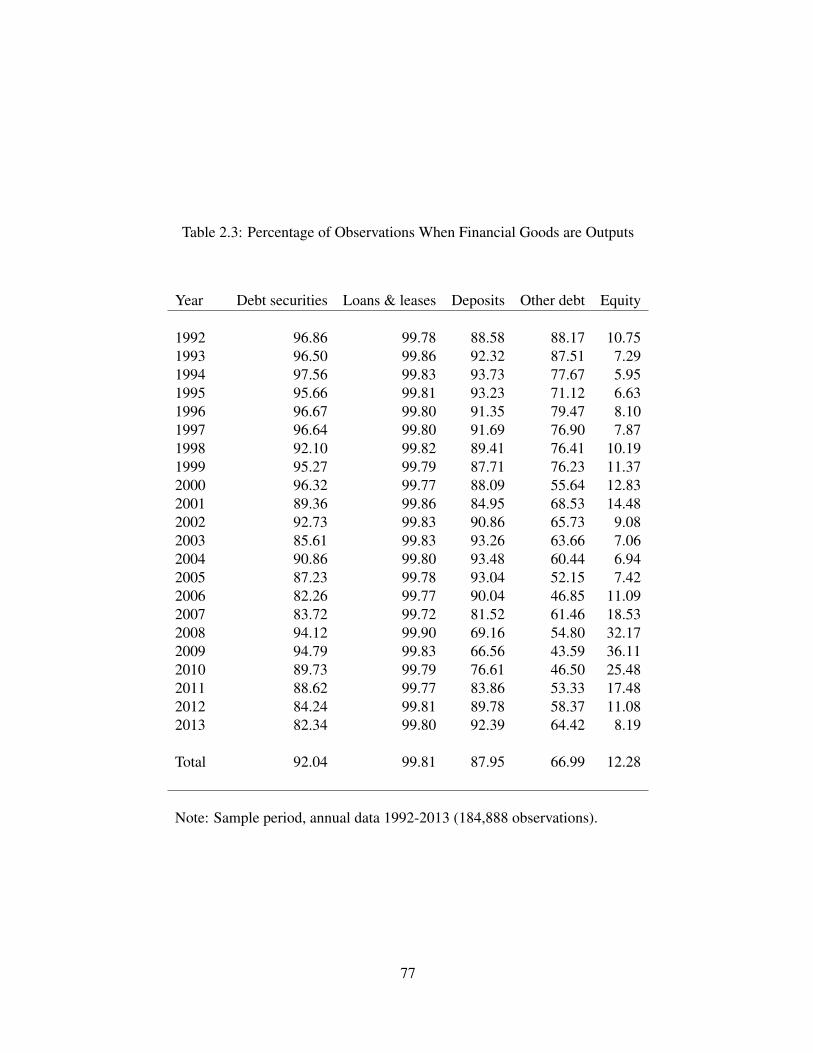
Table 2.3: Percentage of Observations When Financial Goods are Outputs

Year Debt securities Loans & leases Deposits Other debt Equity

1992 96.86 99.78 88.58 88.17 10.751993 96.50 99.86 92.32 87.51 7.291994 97.56 99.83 93.73 77.67 5.951995 95.66 99.81 93.23 71.12 6.631996 96.67 99.80 91.35 79.47 8.101997 96.64 99.80 91.69 76.90 7.871998 92.10 99.82 89.41 76.41 10.191999 95.27 99.79 87.71 76.23 11.372000 96.32 99.77 88.09 55.64 12.832001 89.36 99.86 84.95 68.53 14.482002 92.73 99.83 90.86 65.73 9.082003 85.61 99.83 93.26 63.66 7.062004 90.86 99.80 93.48 60.44 6.942005 87.23 99.78 93.04 52.15 7.422006 82.26 99.77 90.04 46.85 11.092007 83.72 99.72 81.52 61.46 18.532008 94.12 99.90 69.16 54.80 32.172009 94.79 99.83 66.56 43.59 36.112010 89.73 99.79 76.61 46.50 25.482011 88.62 99.77 83.86 53.33 17.482012 84.24 99.81 89.78 58.37 11.082013 82.34 99.80 92.39 64.42 8.19

Total 92.04 99.81 87.95 66.99 12.28

Note: Sample period, annual data 1992-2013 (184,888 observations).

77

Tabl

e2.

4:U

serC

osts

Ave

rage

dA

cros

sB

anks

(and

the

Dis

coun

tRat

e)

Year

Deb

tsec

uriti

esLo

ans

&le

ases

Dep

osits

Oth

erde

btEq

uity

Dis

coun

trat

e

1992

�0.

0182

3�

0.03

693

�0.

0039

5�

0.01

695

0.03

450

0.04

329

1993

�0.

0160

5�

0.03

564

�0.

0053

8�

0.01

425

0.05

032

0.03

730

1994

�0.

0155

4�

0.03

512

�0.

0054

5�

0.00

768

0.05

010

0.03

655

1995

�0.

0143

9�

0.03

596

�0.

0053

6�

0.00

579

0.04

603

0.04

274

1996

�0.

0149

3�

0.03

511

�0.

0050

8�

0.01

215

0.04

567

0.04

282

1997

�0.

0160

9�

0.03

484

�0.

0052

5�

0.01

018

0.04

446

0.04

319

1998

�0.

0140

8�

0.03

611

�0.

0048

6�

0.01

078

0.04

665

0.04

219

1999

�0.

0154

8�

0.03

409

�0.

0046

4�

0.00

958

0.05

045

0.04

007

2000

�0.

0172

6�

0.03

471

�0.

0049

60.

0021

10.

0447

70.

0436

420

01�

0.01

524

�0.

0363

4�

0.00

428

�0.

0067

30.

0405

90.

0399

020

02�

0.01

634

�0.

0365

4�

0.00

660

�0.

0052

70.

0567

60.

0304

620

03�

0.01

067

�0.

0367

4�

0.00

732

�0.

0026

50.

0605

40.

0251

420

04�

0.01

245

�0.

0355

7�

0.00

793

�0.

0010

00.

0679

00.

0230

020

05�

0.01

060

�0.

0364

7�

0.00

818

0.00

379

0.07

049

0.02

682

2006

�0.

0099

7�

0.03

769

�0.

0071

70.

0085

60.

0608

20.

0331

120

07�

0.01

234

�0.

0385

5�

0.00

457

�0.

0005

90.

0415

30.

0350

320

08�

0.02

333

�0.

0427

2�

0.00

005

0.00

267

�0.

0177

30.

0242

020

09�

0.02

636

�0.

0480

50.

0015

90.

0088

0�

0.25

790

0.01

559

2010

�0.

0186

1�

0.04

904

�0.

0021

80.

0083

2�

0.05

807

0.01

465

2011

�0.

0149

8�

0.04

823

�0.

0051

90.

0042

00.

0001

90.

0142

220

12�

0.01

152

�0.

0462

3�

0.00

765

0.00

231

0.04

677

0.01

397

2013

�0.

0089

8�

0.04

376

�0.

0084

1�

0.00

004

0.05

340

0.01

309

78

Tabl

e2.

5:Tr

ansl

ogPa

ram

eter

Estim

ates

Ass

ets

Less

than

$100

mill

ion

$1bi

llion

toM

ore

than

Para

met

erA

llba

nks

$100

mill

ion

to$1

billi

on$1

0bi

llion

$10

billi

on

a 1�

0.11

0(0.7

57)

�0.

107(0.0

13)

0.94

9(2.7

33)

�0.

460(2.2

84)

0.49

8(0.0

04)

a 20.

038(0.5

62)

0.74

9(0.1

35)

�0.

588(1.2

65)

1.11

0(0.2

46)

0.17

2(0.5

54)

a 30.

571(0.2

12)

0.03

6(0.0

48)

0.54

9(0.4

88)

0.77

2(3.0

47)

0.09

5(0.0

12)

a 40.

752(0.0

09)

0.50

3(0.1

23)

0.18

3(1.2

54)

�0.

369(0.1

67)

0.26

6(0.5

85)

b 11

�0.

000(0.0

00)

�0.

479(0.1

40)

�0.

141(1.2

47)

�0.

000(0.0

02)

�0.

053(0.0

01)

b 21

0.58

2(0.0

28)

0.41

8(0.1

91)

0.42

4(0.0

49)

0.09

4(0.3

63)

�0.

371(0.4

86)

b 22

�0.

190(0.5

24)

�0.

000(0.0

00)

�0.

168(0.1

77)

�0.

175(0.2

37)

0.35

2(0.0

42)

b 31

�0.

887(0.1

70)

0.53

9(0.0

24)

�0.

582(2.1

69)

�0.

510(0.4

42)

0.28

4(0.3

20)

b 32

0.13

9(0.2

42)

0.23

3(0.0

64)

�0.

039(0.3

28)

0.10

1(0.1

93)

�0.

435(0.1

61)

b 33

�0.

417(0.9

40)

�0.

040(0.0

27)

�0.

261(0.1

72)

�0.

163(0.6

95)

�0.

346(0.0

82)

b 41

0.09

4(0.5

57)

�0.

641(0.4

79)

0.28

2(0.8

97)

0.20

2(0.5

03)

0.19

1(0.2

25)

b 42

�0.

438(0.2

08)

�0.

353(0.0

64)

0.24

6(0.5

31)

�0.

008(0.0

68)

0.03

0(0.1

06)

b 43

0.46

9(0.4

25)

�0.

309(0.1

50)

�0.

006(0.0

78)

0.06

9(0.3

44)

0.29

1(0.0

82)

b 44

0.19

4(2.4

70)

�0.

386(0.2

10)

�0.

193(0.7

13)

�0.

009(0.5

40)

�0.

183(0.1

41)

Obs

erva

tions

184,

888

96,3

4077,9

458,

874

1,72

9

Viol

atio

ns(%

)C

onve

xity

6997

9899

81M

onot

onic

ity40

3535

3524

Not

e:St

anda

rder

rors

inpa

rent

hese

s.1=

Deb

tsec

uriti

es,2

=Lo

ans

and

leas

es,3

=D

epos

its,4

=O

ther

debt

,5=

Equi

ty.

79

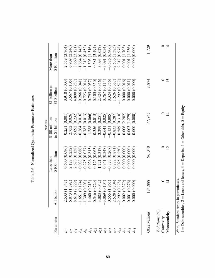
Tabl

e2.

6:N

orm

aliz

edQ

uadr

atic

Para

met

erEs

timat

es

Ass

ets

Less

than

$100

mill

ion

$1bi

llion

toM

ore

than

Para

met

erA

llba

nks

$100

mill

ion

to$1

billi

on$1

0bi

llion

$10

billi

on

b 12.

533(1.3

47)

0.60

0(0.0

96)

0.25

1(0.0

01)

0.91

8(0.0

03)

2.55

9(3.7

64)

b 26.

873(1.8

92)

2.12

7(0.2

32)

2.75

2(0.0

26)

3.56

7(0.1

05)

6.90

9(2.2

46)

b 38.

619(2.2

29)

2.67

3(0.1

58)

5.09

2(0.2

32)

4.89

0(0.2

87)

8.66

0(3.1

21)

b 4�

1.65

1(0.1

74)

�0.

033(0.0

86)

�0.

264(0.0

16)

�0.

266(0.0

41)

�1.

664(0.1

43)

b 5�

1.30

9(0.3

03)

�0.

275(0.0

37)

�0.

783(0.0

13)

�0.

723(0.0

14)

�1.

313(0.4

52)

k 11

1.46

0(0.2

13)

0.92

6(0.8

15)

�1.

288(0.0

66)

0.79

5(0.0

57)

1.50

3(1.3

16)

k 21

�0.

546(0.7

29)

0.12

5(0.0

63)

�0.

356(0.0

15)

0.10

5(0.3

50)

�0.

581(3.4

94)

k 22

3.08

3(0.0

42)

�1.

721(0.3

17)

3.29

9(0.2

51)

�2.

424(0.3

56)

3.09

3(0.0

27)

k 31

�3.

069(0.1

04)

0.34

1(0.3

47)

�0.

641(0.0

25)

0.76

7(0.1

14)

�3.

091(0.0

34)

k 32

0.55

5(1.9

65)

�0.

373(0.2

67)

�0.

131(0.8

05)

0.32

4(0.7

56)

�0.

576(6.9

06)

k 33

2.52

8(0.7

04)

0.27

2(0.8

71)

�0.

833(0.2

87)

1.52

6(0.3

87)

�2.

536(1.5

85)

k 41

�2.

292(0.7

78)

0.02

5(0.2

50)

0.58

9(0.3

10)

�1.

292(0.5

77)

2.31

7(0.9

78)

k 42

�0.

002(0.3

79)

0.00

0(0.0

00)

�0.

006(2.2

02)

0.00

0(0.0

16)

0.00

1(1.7

03)

k 43

0.00

1(0.2

76)

�0.

000(0.0

00)

0.00

3(1.2

79)

�0.

000(0.0

11)

�0.

001(1.2

36)

k 44

0.00

0(0.0

00)

0.00

0(0.0

00)

�0.

000(0.0

00)

0.00

0(0.0

00)

�0.

000(0.0

00)

Obs

erva

tions

184,

888

96,3

4077,9

458,

874

1,72

9

Viol

atio

ns(%

)C

onve

xity

00

00

0M

onot

onic

ity14

1214

1514

Not

e:St

anda

rder

rors

inpa

rent

hese

s.1=

Deb

tsec

uriti

es,2

=Lo

ans

and

leas

es,3

=D

epos

its,4

=O

ther

debt

,5=

Equi

ty.

80

Tabl

e2.

7:G

ener

aliz

edB

arne

ttPa

ram

eter

Estim

ates

Ass

ets

Less

than

$100

mill

ion

$1bi

llion

toM

ore

than

Para

met

erA

llba

nks

$100

mill

ion

to$1

billi

on$1

0bi

llion

$10

billi

on

a 11

1.71

9(0

.048

)-0

.980

(0.0

00)

1.10

6(0

.250

)1.

137

(0.8

12)

1.20

8(0

.445

)a 1

20.

523

(0.0

31)

-0.2

14(0

.004

)0.

314

(0.4

30)

0.11

1(4

.522

)-0

.000

(0.0

00)

a 13

0.09

0(0

.035

)-0

.206

(0.0

15)

-0.0

00(0

.000

)-0

.000

(0.0

00)

0.38

6(0

.063

)a 1

40.

419

(0.0

07)

-0.0

03(0

.003

)-0

.000

(0.0

01)

-0.2

14(0

.009

)-0

.456

(0.4

47)

a 15

0.45

1(0

.080

)0.

006

(0.0

05)

0.00

0(0

.000

)0.

000

(0.0

00)

-0.3

19(0

.327

)a 2

2-2

.526

(0.0

64)

1.37

7(0

.001

)1.

639

(0.1

59)

1.86

5(0

.424

)-1

.970

(0.9

44)

a 23

0.00

3(0

.002

)0.

175

(0.0

10)

-0.0

00(0

.000

)0.

000

(0.0

00)

-0.0

00(0

.000

)a 2

40.

173

(0.0

84)

0.00

9(0

.009

)0.

049

(0.0

67)

-0.0

00(0

.000

)-0

.000

(0.0

00)

a 25

-0.0

07(0

.002

)0.

028

(0.0

09)

-0.1

40(0

.081

)-0

.130

(0.1

48)

-0.1

65(0

.261

)a 3

3-3

.110

(0.1

88)

1.81

4(0

.001

)2.

231

(0.1

41)

2.54

8(0

.362

)2.

366

(0.3

95)

a 34

0.22

8(0

.108

)-0

.006

(0.0

06)

-0.0

00(0

.000

)0.

000

(0.0

00)

0.00

0(0

.000

)a 3

51.

237

(0.1

03)

-0.6

43(0

.000

)0.

836

(0.0

27)

0.96

0(0

.176

)0.

683

(0.0

66)

a 44

0.80

3(0

.193

)0.

198

(0.0

00)

0.29

7(0

.049

)0.

554

(0.0

18)

0.80

9(0

.671

)a 4

5-0

.046

(0.0

39)

-0.0

58(0

.002

)-0

.000

(0.0

00)

-0.0

00(0

.000

)0.

000

(0.0

00)

a 55

-0.0

68(0

.065

)0.

000

(0.0

00)

0.00

0(0

.000

)-0

.000

(0.0

00)

0.00

0(0

.000

)a 1

23-0

.000

(0.0

00)

0.00

0(0

.000

)-0

.000

(0.0

00)

0.00

0(0

.000

)0.

000

(0.0

00)

a 124

-0.0

00(0

.000

)-0

.001

(0.0

00)

-0.0

00(0

.000

)0.

000

(0.0

00)

0.00

0(0

.000

)a 1

250.

000

(0.0

00)

0.00

0(0

.000

)0.

000

(0.0

00)

0.00

0(0

.000

)-0

.000

(0.0

00)

a 134

-0.0

02(0

.001

)0.

000

(0.0

00)

-0.0

00(0

.000

)0.

000

(0.0

00)

-0.0

00(0

.000

)a 1

350.

000

(0.0

00)

-0.0

00(0

.000

)0.

000

(0.0

00)

0.00

0(0

.000

)0.

000

(0.0

00)

a 145

0.00

2(0

.001

)0.

000

(0.0

00)

0.00

0(0

.000

)-0

.000

(0.0

00)

0.00

0(0

.000

)a 1

560.

000

(0.0

00)

0.00

0(0

.000

)-0

.000

(0.0

00)

0.00

0(0

.000

)0.

000

(0.0

00)

a 155

-0.0

00(0

.000

)-0

.000

(0.0

00)

-0.0

00(0

.000

)-0

.000

(0.0

00)

0.00

0(0

.000

)a 2

130.

001

(0.0

01)

-0.0

00(0

.000

)0.

000

(0.0

00)

-0.0

00(0

.000

)0.

000

(0.0

00)

a 214

-0.0

00(0

.000

)0.

000

(0.0

00)

0.00

0(0

.000

)-0

.000

(0.0

00)

0.00

0(0

.000

)a 2

15-0

.000

(0.0

00)

-0.0

00(0

.000

)0.

000

(0.0

00)

0.00

0(0

.000

)0.

000

(0.0

00)

a 234

-0.0

00(0

.000

)-0

.000

(0.0

00)

0.00

0(0

.000

)0.

000

(0.0

00)

-0.0

00(0

.000

)a 2

350.

001

(0.0

00)

0.00

0(0

.000

)0.

001

(0.0

18)

0.00

0(0

.000

)-0

.000

(0.0

00)

81

Tabl

e7

(Con

t’d).

Gen

eral

ized

Bar

nett

Para

met

erEs

timat

es

Ass

ets

Less

than

$100

mill

ion

$1bi

llion

toM

ore

than

Para

met

erA

llba

nks

$100

mill

ion

to$1

billi

on$1

0bi

llion

$10

billi

on

a 245

0.00

3(0

.001

)-0

.000

(0.0

00)

-0.0

00(0

.000

)0.

000

(0.0

00)

-0.0

78(0

.038

)a 2

56-0

.004

(0.0

02)

-0.0

00(0

.000

)-0

.000

(0.0

00)

-0.0

00(0

.000

)-0

.000

(0.0

00)

a 255

0.00

3(0

.000

)0.

001

(0.0

01)

0.00

0(0

.000

)0.

000

(0.0

00)

0.00

0(0

.000

)a 3

120.

013

(0.0

01)

-0.0

00(0

.000

)0.

000

(0.0

00)

-0.0

00(0

.000

)-0

.000

(0.0

00)

a 314

-0.0

00(0

.000

)0.

000

(0.0

00)

0.00

0(0

.000

)0.

000

(0.0

00)

-0.0

00(0

.000

)a 3

15-0

.005

(0.0

01)

-0.0

00(0

.000

)0.

002

(0.0

04)

-0.0

09(0

.297

)-0

.000

(0.0

00)

a 324

-0.0

02(0

.001

)0.

000

(0.0

00)

0.00

0(0

.000

)0.

000

(0.0

00)

0.00

0(0

.000

)a 3

250.

001

(0.0

00)

-0.0

00(0

.000

)-0

.000

(0.0

00)

-0.0

00(0

.000

)-0

.000

(0.0

00)

a 345

0.00

2(0

.001

)0.

000

(0.0

00)

0.00

0(0

.000

)0.

000

(0.0

00)

-0.0

00(0

.000

)a 3

56-0

.007

(0.0

05)

0.00

0(0

.000

)-0

.000

(0.0

00)

0.00

0(0

.000

)-0

.000

(0.0

00)

a 355

-0.0

00(0

.000

)-0

.000

(0.0

00)

-0.0

00(0

.000

)0.

000

(0.0

00)

-0.0

00(0

.000

)a 4

12-0

.000

(0.0

00)

0.00

0(0

.000

)-0

.000

(0.0

00)

-0.0

00(0

.000

)-0

.000

(0.0

00)

a 413

0.00

0(0

.000

)0.

000

(0.0

00)

0.00

0(0

.000

)-0

.000

(0.0

00)

0.00

0(0

.000

)a 4

150.

000

(0.0

00)

-0.0

00(0

.000

)0.

000

(0.0

00)

0.00

0(0

.000

)-0

.000

(0.0

00)

a 423

-0.0

01(0

.000

)0.

000

(0.0

00)

-0.0

00(0

.000

)0.

000

(0.0

00)

-0.0

00(0

.000

)a 4

25-0

.001

(0.0

00)

-0.0

00(0

.000

)-0

.000

(0.0

00)

-0.0

00(0

.000

)0.

000

(0.0

00)

a 435

-0.0

00(0

.000

)0.

000

(0.0

00)

-0.0

00(0

.000

)-0

.000

(0.0

00)

-0.0

00(0

.000

)

Obs

erva

tions

184,

888

96,3

4077,9

458,

874

1,72

9

Viol

atio

ns(%

)C

onve

xity

00

00

0M

onot

onic

ity7

014

2614

Not

e:St

anda

rder

rors

inpa

rent

hese

s.1=

Deb

tsec

uriti

es,2

=Lo

ans

and

leas

es,3

=D

epos

its,4

=O

ther

debt

,5=

Equi

ty.

82

Tabl

e2.

8:El

astic

ities

ofTr

ansf

orm

atio

n,A

llB

anks

Elas

ticiti

esof

Tran

sfor

mat

ion

Fina

ncia

lgoo

di

Mod

els i

Ss i

Ls i

Ds i

Os i

E

Deb

tN

Q1.

898

(0.2

27)

secu

ritie

s(S

)G

B2.

469

(0.0

36)

Loan

sN

Q0.

003

(0.0

17)

0.02

5(0

.005

)an

dLe

ases

(L)

GB

-0.1

27(0

.016

)0.

019

(0.0

02)

Dep

osits

(D)

NQ

1.04

1(0

.083

)0.

070

(0.0

17)

0.75

6(0

.025

)G

B-0

.010

(0.0

09)

-0.0

00(0

.000

)3.

358

(0.0

10)

Oth

erde

bt(O

)N

Q-1

5.86

7(0

.505

)-0

.998

(0.1

05)

-11.

321

(0.9

76)

169.

785

(34.

796)

GB

-1.6

91(1

.273

)-0

.057

(0.0

25)

-0.2

76(0

.113

)9.

358

(11.

291)

Equi

ty(E

)N

Q1.

138

(0.2

14)

0.09

7(0

.032

)0.

882

(0.1

26)

-13.

166

(0.2

90)

1.04

1(0

.265

)G

B0.

700

(0.2

83)

0.00

0(0

.000

)2.

890

(0.0

06)

0.03

1(0

.038

)3.

022

(0.2

89)

Not

e:Sa

mpl

epe

riod,

annu

alda

ta19

92-2

013

(184,8

88ob

serv

atio

ns).

83

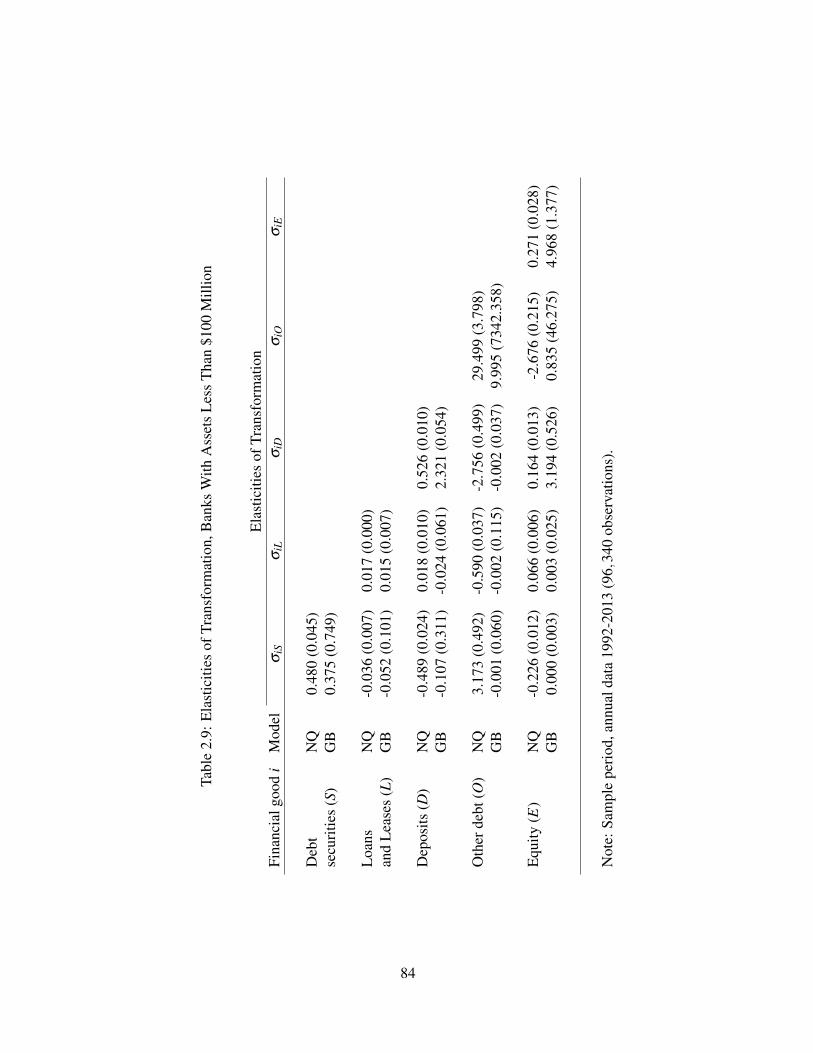
Tabl

e2.

9:El

astic

ities

ofTr

ansf

orm

atio

n,B

anks

With

Ass

ets

Less

Than

$100

Mill

ion

Elas

ticiti

esof

Tran

sfor

mat

ion

Fina

ncia

lgoo

di

Mod

els i

Ss i

Ls i

Ds i

Os i

E

Deb

tN

Q0.

480

(0.0

45)

secu

ritie

s(S

)G

B0.

375

(0.7

49)

Loan

sN

Q-0

.036

(0.0

07)

0.01

7(0

.000

)an

dLe

ases

(L)

GB

-0.0

52(0

.101

)0.

015

(0.0

07)

Dep

osits

(D)

NQ

-0.4

89(0

.024

)0.

018

(0.0

10)

0.52

6(0

.010

)G

B-0

.107

(0.3

11)

-0.0

24(0

.061

)2.

321

(0.0

54)

Oth

erde

bt(O

)N

Q3.

173

(0.4

92)

-0.5

90(0

.037

)-2

.756

(0.4

99)

29.4

99(3

.798

)G

B-0

.001

(0.0

60)

-0.0

02(0

.115

)-0

.002

(0.0

37)

9.99

5(7

342.

358)

Equi

ty(E

)N

Q-0

.226

(0.0

12)

0.06

6(0

.006

)0.

164

(0.0

13)

-2.6

76(0

.215

)0.

271

(0.0

28)

GB

0.00

0(0

.003

)0.

003

(0.0

25)

3.19

4(0

.526

)0.

835

(46.

275)

4.96

8(1

.377

)

Not

e:Sa

mpl

epe

riod,

annu

alda

ta19

92-2

013

(96,

340

obse

rvat

ions

).

84

Tabl

e2.

10:E

last

iciti

esof

Tran

sfor

mat

ion,

Ban

ksW

ithA

sset

sB

etw

een

$100

Mill

ion

and

$1B

illio

n

Elas

ticiti

esof

Tran

sfor

mat

ion

Fina

ncia

lgoo

di

Mod

els i

Ss i

Ls i

Ds i

Os i

E

Deb

tN

Q0.

452

(0.1

70)

secu

ritie

s(S

)G

B0.

509

(1.4

25)

Loan

sN

Q-0

.036

(0.0

22)

0.01

6(0

.008

)an

dLe

ases

(L)

GB

-0.0

88(0

.238

)0.

023

(0.0

48)

Dep

osits

(D)

NQ

-0.7

35(0

.210

)0.

130

(0.0

22)

1.59

9(0

.050

)G

B-0

.000

(0.0

00)

-0.0

00(0

.000

)2.

006

(0.3

14)

Oth

erde

bt(O

)N

Q-1

.582

(3.0

17)

-0.9

92(0

.881

)-3

.647

(5.3

35)

101.

493

(50.

103)

GB

-0.0

00(0

.001

)-0

.027

(0.1

02)

-0.0

00(0

.000

)1.

786

(9.8

08)

Equi

ty(E

)N

Q-0

.607

(0.1

24)

0.14

0(0

.018

)1.

502

(0.2

06)

-5.8

26(5

.334

)1.

473

(0.3

24)

GB

0.00

0(0

.000

)0.

034

(0.0

33)

2.35

2(0

.242

)0.

000

(0.0

00)

2.92

0(0

.025

)

Not

e:Sa

mpl

epe

riod,

annu

alda

ta19

92-2

013

(8,8

74ob

serv

atio

ns).

85

Tabl

e2.

11:E

last

iciti

esof

Tran

sfor

mat

ion,

Ban

ksW

ithA

sset

sB

etw

een

$1B

illio

nan

d$1

0B

illio

n

Elas

ticiti

esof

Tran

sfor

mat

ion

Fina

ncia

lgoo

di

Mod

els i

Ss i

Ls i

Ds i

Os i

E

Deb

tN

Q0.

116

(0.0

69)

secu

ritie

s(S

)G

B0.

153

(3.9

14)

Loan

sN

Q0.

006

(0.0

29)

0.03

1(0

.006

)an

dLe

ases

(L)

GB

-0.0

09(0

.735

)0.

007

(0.1

22)

Dep

osits

(D)

NQ

-0.1

19(0

.123

)0.

142

(0.0

27)

0.83

6(0

.036

)G

B0.

000

(0.0

00)

-0.0

00(0

.000

)1.

559

(0.3

45)

Oth

erde

bt(O

)N

Q-0

.385

(0.3

84)

-0.6

15(0

.098

)-2

.481

(0.4

44)

12.8

37(1

.974

)G

B-0

.737

(0.1

07)

-0.0

00(0

.013

)-0

.000

(0.0

00)

5.15

9(1

.124

)

Equi

ty(E

)N

Q-0

.062

(0.1

33)

0.17

6(0

.017

)0.

927

(0.0

68)

-3.2

68(0

.271

)1.

077

(0.1

23)

GB

0.00

0(0

.000

)0.

021

(0.0

52)

1.94

5(0

.241

)0.

000

(0.0

01)

2.50

8(0

.084

)

Not

e:Sa

mpl

epe

riod,

annu

alda

ta19

92-2

013

(8,8

74ob

serv

atio

ns).

86

Tabl

e2.

12:E

last

iciti

esof

Tran

sfor

mat

ion,

Ban

ksW

ithA

sset

sM

ore

Than

$10

Bill

ion

Elas

ticiti

esof

Tran

sfor

mat

ion

Fina

ncia

lgoo

di

Mod

els i

Ss i

Ls i

Ds i

Os i

E

Deb

tN

Q1.

898

(0.2

27)

secu

ritie

s(S

)G

B2.

497

(4.7

06)

Loan

sN

Q0.

003

(0.0

17)

0.02

5(0

.005

)an

dLe

ases

(L)

GB

0.00

0(0

.000

)0.

009

(0.0

18)

Dep

osits

(D)

NQ

1.04

1(0

.083

)0.

070

(0.0

17)

0.75

6(0

.025

)G

B-0

.231

(0.0

80)

0.00

0(0

.000

)0.

686

(0.1

20)

Oth

erde

bt(O

)N

Q-1

5.86

7(0

.505

)-0

.998

(0.1

05)

-11.

321

(0.9

76)

169.

785

(34.

796)

GB

-3.4

94(5

.084

)0.

000

(0.0

00)

-0.0

54(0

.121

)16

.892

(0.0

39)

Equi

ty(E

)N

Q1.

138

(0.2

14)

0.09

7(0

.032

)0.

882

(0.1

26)

-13.

166

(0.2

90)

1.04

1(0

.265

)G

B0.

948

(1.6

75)

0.04

9(0

.101

)1.

297

(0.2

62)

0.00

0(0

.000

)3.

899

(0.0

81)

Not

e:Sa

mpl

epe

riod,

annu

alda

ta19

92-2

013

(1,7

29ob

serv

atio

ns).

87

Tabl

e2.

13:P

rice

Elas

ticiti

es,A

llB

anks

Pric

eel

astic

ities

Fina

ncia

lgoo

di

Mod

elh i

Sh i

Lh i

Dh i

Oh i

E

Deb

tN

Q0.

377

(0.0

31)

0.12

2(0

.020

)0.

369

(0.0

15)

-0.5

93(0

.011

)-0

.274

(0.0

55)

secu

ritie

s(S

)G

B0.

281

(0.0

18)

-0.1

11(0

.017

)-0

.002

(0.0

01)

-0.0

52(0

.004

)-0

.117

(0.0

38)

Loan

sN

Q0.

010

(0.0

02)

0.03

4(0

.003

)0.

025

(0.0

02)

-0.0

40(0

.002

)-0

.029

(0.0

05)

and

Leas

es(L

)G

B-0

.014

(0.0

01)

0.01

6(0

.001

)-0

.000

(0.0

00)

-0.0

02(0

.002

)-0

.000

(0.0

00)

Dep

osits

(D)

NQ

0.17

8(0

.004

)0.

150

(0.0

09)

0.22

0(0

.004

)-0

.354

(0.0

15)

-0.1

94(0

.023

)G

B-0

.001

(0.0

01)

-0.0

00(0

.000

)0.

492

(0.0

25)

-0.0

09(0

.009

)-0

.482

(0.0

35)

Oth

erde

bt(O

)N

Q-0

.589

(0.0

25)

-0.4

93(0

.036

)-0

.726

(0.0

01)

1.16

8(0

.027

)0.

640

(0.0

89)

GB

-0.1

93(0

.119

)-0

.050

(0.0

20)

-0.0

40(0

.015

)0.

288

(0.0

79)

-0.0

05(0

.006

)

Equi

ty(E

)N

Q0.

109

(0.0

23)

0.14

2(0

.026

)0.

160

(0.0

24)

-0.2

57(0

.033

)-0

.154

(0.0

41)

GB

0.08

0(0

.036

)0.

000

(0.0

00)

0.42

3(0

.030

)0.

001

(0.0

02)

-0.5

04(0

.008

)

Not

e:Sa

mpl

epe

riod,

annu

alda

ta19

92-2

013

(184,8

88ob

serv

atio

ns).

88

Tabl

e2.

14:P

rice

Elas

ticiti

es,B

anks

With

Ass

ets

Less

Than

$100

Mill

ion

Pric

eel

astic

ities

Fina

ncia

lgoo

di

Mod

elh i

Sh i

Lh i

Dh i

Oh i

E

Deb

tN

Q0.

064

(0.0

06)

-0.0

31(0

.006

)-0

.081

(0.0

04)

0.01

4(0

.002

)0.

034

(0.0

02)

secu

ritie

s(S

)G

B0.

058

(0.1

23)

-0.0

41(0

.075

)-0

.016

(0.0

49)

-0.0

00(0

.000

)-0

.000

(0.0

00)

Loan

sN

Q-0

.005

(0.0

01)

0.01

4(0

.000

)0.

003

(0.0

02)

-0.0

03(0

.000

)-0

.010

(0.0

01)

and

Leas

es(L

)G

B-0

.008

(0.0

17)

0.01

2(0

.005

)-0

.004

(0.0

09)

-0.0

00(0

.000

)-0

.000

(0.0

03)

Dep

osits

(D)

NQ

-0.0

65(0

.003

)0.

015

(0.0

09)

0.08

7(0

.001

)-0

.012

(0.0

02)

-0.0

25(0

.002

)G

B-0

.017

(0.0

50)

-0.0

19(0

.048

)0.

356

(0.0

30)

-0.0

00(0

.000

)-0

.321

(0.0

28)

Oth

erde

bt(O

)N

Q0.

422

(0.0

66)

-0.5

01(0

.032

)-0

.455

(0.0

84)

0.12

7(0

.015

)0.

408

(0.0

34)

GB

-0.0

00(0

.004

)-0

.002

(0.0

28)

-0.0

00(0

.001

)0.

086

(0.2

39)

-0.0

84(0

.272

)

Equi

ty(E

)N

Q-0

.030

(0.0

02)

0.05

6(0

.005

)0.

027

(0.0

02)

-0.0

12(0

.001

)-0

.041

(0.0

04)

GB

0.00

0(0

.000

)0.

002

(0.0

22)

0.49

0(0

.001

)0.

007

(0.0

24)

-0.5

00(0

.000

)

Not

e:Sa

mpl

epe

riod,

annu

alda

ta19

92-2

013

(96,

340

obse

rvat

ions

).

89

Tabl

e2.

15:P

rice

Elas

ticiti

es,B

anks

With

Ass

ets

Bet

wee

n$1

00M

illio

nan

d$1

Bill

ion

Pric

eel

astic

ities

Fina

ncia

lgoo

di

Mod

elh i

Sh i

Lh i

Dh i

Oh i

E

Deb

tN

Q0.

052

(0.0

20)

-0.0

32(0

.020

)-0

.149

(0.0

43)

-0.0

08(0

.014

)0.

136

(0.0

29)

secu

ritie

s(S

)G

B0.

072

(0.1

87)

-0.0

72(0

.187

)-0

.000

(0.0

00)

-0.0

00(0

.000

)-0

.000

(0.0

00)

Loan

sN

Q-0

.004

(0.0

03)

0.01

4(0

.007

)0.

026

(0.0

04)

-0.0

05(0

.005

)-0

.032

(0.0

04)

and

Leas

es(L

)G

B-0

.012

(0.0

32)

0.01

8(0

.039

)-0

.000

(0.0

00)

-0.0

00(0

.001

)-0

.006

(0.0

06)

Dep

osits

(D)

NQ

-0.0

85(0

.024

)0.

118

(0.0

20)

0.32

3(0

.009

)-0

.018

(0.0

29)

-0.3

37(0

.043

)G

B-0

.000

(0.0

00)

-0.0

00(0

.000

)0.

403

(0.0

45)

-0.0

00(0

.000

)-0

.403

(0.0

45)

Oth

erde

bt(O

)N

Q-0

.183

(0.3

50)

-0.8

94(0

.795

)-0

.737

(1.0

79)

0.50

7(0

.313

)1.

308

(1.2

11)

GB

-0.0

00(0

.000

)-0

.022

(0.0

53)

-0.0

00(0

.000

)0.

022

(0.0

53)

-0.0

00(0

.000

)

Equi

ty(E

)N

Q-0

.070

(0.0

14)

0.12

7(0

.016

)0.

303

(0.0

41)

-0.0

29(0

.030

)-0

.331

(0.0

69)

GB

0.00

0(0

.000

)0.

028

(0.0

29)

0.47

2(0

.029

)0.

000

(0.0

00)

-0.5

00(0

.000

)

Not

e:Sa

mpl

epe

riod,

annu

alda

ta19

92-2

013

(77,

945

obse

rvat

ions

).

90

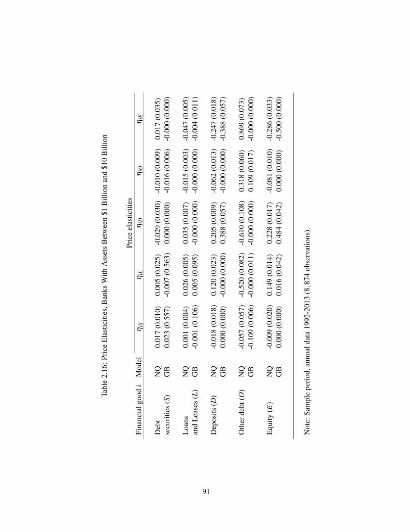
Tabl

e2.

16:P

rice

Elas

ticiti

es,B

anks

With

Ass

ets

Bet

wee

n$1

Bill

ion

and

$10

Bill

ion

Pric

eel

astic

ities

Fina

ncia

lgoo

di

Mod

elh i

Sh i

Lh i

Dh i

Oh i

E

Deb

tN

Q0.

017

(0.0

10)

0.00

5(0

.025

)-0

.029

(0.0

30)

-0.0

10(0

.009

)0.

017

(0.0

35)

secu

ritie

s(S

)G

B0.

023

(0.5

57)

-0.0

07(0

.563

)0.

000

(0.0

00)

-0.0

16(0

.006

)-0

.000

(0.0

00)

Loan

sN

Q0.

001

(0.0

04)

0.02

6(0

.005

)0.

035

(0.0

07)

-0.0

15(0

.003

)-0

.047

(0.0

05)

and

Leas

es(L

)G

B-0

.001

(0.1

06)

0.00

5(0

.095

)-0

.000

(0.0

00)

-0.0

00(0

.000

)-0

.004

(0.0

11)

Dep

osits

(D)

NQ

-0.0

18(0

.018

)0.

120

(0.0

23)

0.20

5(0

.009

)-0

.062

(0.0

13)

-0.2

47(0

.018

)G

B0.

000

(0.0

00)

-0.0

00(0

.000

)0.

388

(0.0

57)

-0.0

00(0

.000

)-0

.388

(0.0

57)

Oth

erde

bt(O

)N

Q-0

.057

(0.0

57)

-0.5

20(0

.082

)-0

.610

(0.1

08)

0.31

8(0

.060

)0.

869

(0.0

73)

GB

-0.1

09(0

.006

)-0

.000

(0.0

11)

-0.0

00(0

.000

)0.

109

(0.0

17)

-0.0

00(0

.000

)

Equi

ty(E

)N

Q-0

.009

(0.0

20)

0.14

9(0

.014

)0.

228

(0.0

17)

-0.0

81(0

.010

)-0

.286

(0.0

33)

GB

0.00

0(0

.000

)0.

016

(0.0

42)

0.48

4(0

.042

)0.

000

(0.0

00)

-0.5

00(0

.000

)

Not

e:Sa

mpl

epe

riod,

annu

alda

ta19

92-2

013

(8,8

74ob

serv

atio

ns).

91

Tabl

e2.

17:P

rice

Elas

ticiti

es,B

anks

With

Ass

ets

Mor

eTh

an$1

0B

illio

n

Pric

eel

astic

ities

Fina

ncia

lgoo

di

Mod

elh i

Sh i

Lh i

Dh i

Oh i

E

Deb

tN

Q0.

251

(0.0

30)

0.00

3(0

.015

)0.

309

(0.0

23)

-0.2

05(0

.008

)-0

.357

(0.0

59)

secu

ritie

s(S

)G

B0.

267

(0.3

54)

0.00

0(0

.000

)-0

.065

(0.0

01)

-0.0

80(0

.138

)-0

.122

(0.2

16)

Loan

sN

Q0.

000

(0.0

02)

0.02

2(0

.005

)0.

021

(0.0

05)

-0.0

13(0

.002

)-0

.031

(0.0

09)

and

Leas

es(L

)G

B0.

000

(0.0

00)

0.00

6(0

.014

)0.

000

(0.0

00)

0.00

0(0

.000

)-0

.006

(0.0

14)

Dep

osits

(D)

NQ

0.13

7(0

.011

)0.

061

(0.0

14)

0.22

4(0

.006

)-0

.146

(0.0

02)

-0.2

76(0

.033

)G

B-0

.025

(0.0

03)

0.00

0(0

.000

)0.

192

(0.0

35)

-0.0

01(0

.002

)-0

.166

(0.0

30)

Oth

erde

bt(O

)N

Q-2

.095

(0.0

70)

-0.8

71(0

.085

)-3

.356

(0.3

10)

2.19

3(0

.290

)4.

129

(0.0

06)

GB

-0.3

73(0

.201

)0.

000

(0.0

00)

-0.0

15(0

.037

)0.

388

(0.1

64)

0.00

0(0

.000

)

Equi

ty(E

)N

Q0.

150

(0.0

28)

0.08

5(0

.028

)0.

261

(0.0

36)

-0.1

70(0

.016

)-0

.327

(0.0

75)

GB

0.10

1(0

.129

)0.

035

(0.0

84)

0.36

4(0

.212

)0.

000

(0.0

00)

-0.5

00(0

.000

)

Not

e:Sa

mpl

epe

riod,

annu

alda

ta19

92-2

013

(1,7

29ob

serv

atio

ns).

92

Figu

re2.

1:D

ynam

ics

ofB

ank

Ass

ets

0 1 2 3 4 5 6 7 8 9

1992

19

94

1996

19

98

2000

20

02

2004

20

06

2008

20

10

2012

Figu

re 1

. Dyn

amic

s of B

ank

Ass

ets

Loan

s and

leas

es

Prem

ises

Oth

er a

sset

s

Deb

t sec

uriti

es

93

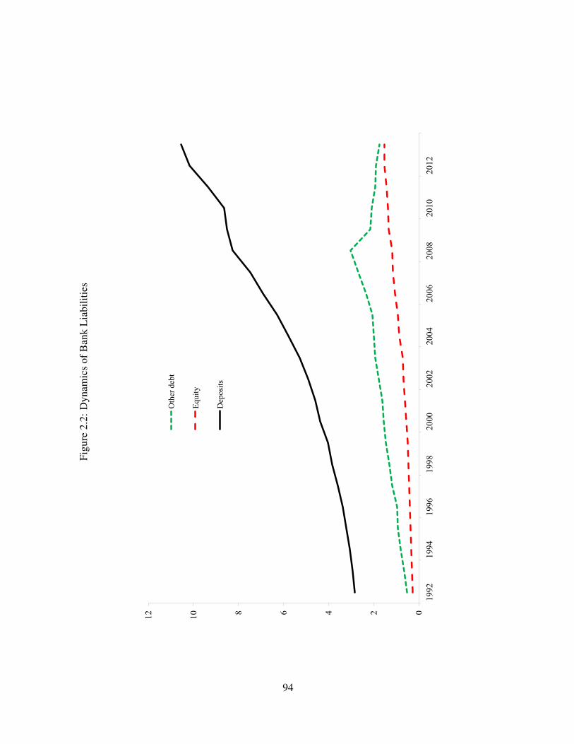
Figu

re2.

2:D

ynam

ics

ofB

ank

Liab

ilitie

s

0 2 4 6 8 10

12

1992

19

94

1996

19

98

2000

20

02

2004

20

06

2008

20

10

2012

Figu

re 2

. Dyn

amic

s of B

ank

Liab

ilitie

s

Oth

er d

ebt

Equi

ty

Dep

osits

94

Figu

re2.

3:A

vera

geR

efer

ence

Dis

coun

tRat

es

0

0.01

0.02

0.03

0.04

0.05

0.06

0.07

1992

199

3 19

94 1

995

1996

199

7 19

98 1

999

2000

200

1 20

02 2

003

2004

200

5 20

06 2

007

2008

200

9 20

10 2

011

2012

201

3

Figu

re 3

. Ave

rage

Ref

eren

ce D

isco

unt R

ates

Deb

t D

epos

its a

nd d

ebt

Dep

osits

, deb

t, an

d eq

uity

Fe

dera

l fun

ds ra

te

95

Figu

re2.

4:O

wn-

pric

eel

astic

ities

ford

ebts

ecur

ities

,hSS

Ͳ0.03

Ͳ0.025

Ͳ0.02

Ͳ0.015

Ͳ0.01

Ͳ0.005

0

0

0.1

0.2

0.3

0.4

0.5

0.6

1992

1994

1996

1998

2000

2002

2004

2006

2008

2010

2012

Figu

re 4

. Ow

n-pr

ice

elas

ticiti

es fo

r deb

t sec

uriti

es, Ș

SS

Gen

eralize

d�Ba

rnett

NQ

User�cost�o

f�deb

t�securities

96

Figu

re2.

5:O

wn-

pric

eel

astic

ities

forl

oans

and

leas

es,h

LL

Ͳ0.06

Ͳ0.05

Ͳ0.04

Ͳ0.03

Ͳ0.02

Ͳ0.01

0

0

0.00

5

0.01

0.01

5

0.02

0.02

5

0.03

0.03

5

0.04

0.04

5

1992

1994

1996

1998

2000

2002

2004

2006

2008

2010

2012

Figu

re 5

. Ow

n-pr

ice

elas

ticiti

es fo

r loa

ns a

nd le

ases

, ȘLL

Gen

eralize

d�Ba

rnett

NQ

User�cost�o

f�loans�and

�leases

97

Figu

re2.

6:O

wn-

pric

eel

astic

ities

ford

epos

its,h

DD

Ͳ0.01

Ͳ0.008

Ͳ0.006

Ͳ0.004

Ͳ0.002

00.00

2

0.00

4

0

0.1

0.2

0.3

0.4

0.5

0.6

0.7

1992

1994

1996

1998

2000

2002

2004

2006

2008

2010

2012

Figu

re 6

. Ow

n-pr

ice

elas

ticiti

es fo

r dep

osits

, ȘD

D

Gen

eralize

d�Ba

rnett

NQ

User�cost�o

f�dep

osits

98

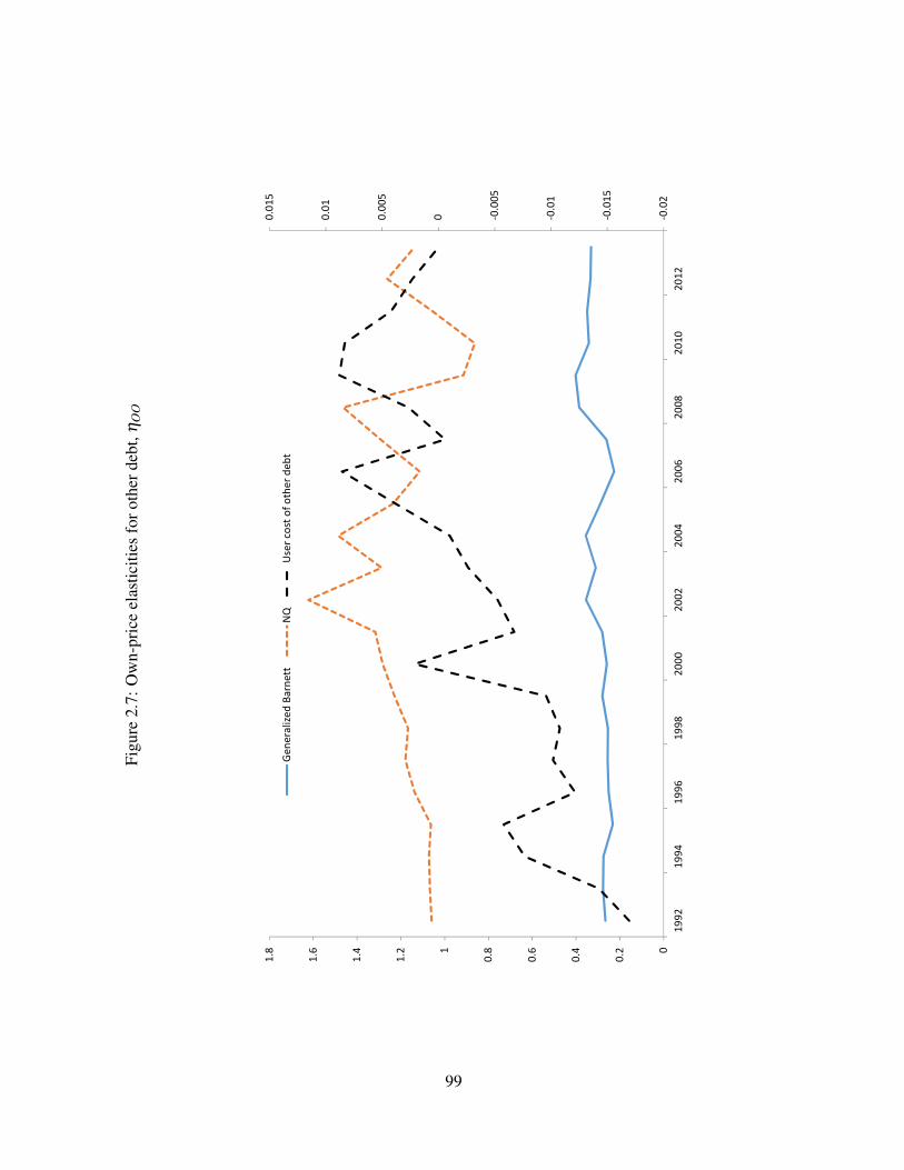
Figu

re2.

7:O

wn-

pric

eel

astic

ities

foro

ther

debt

,hO

O

Ͳ0.02

Ͳ0.015

Ͳ0.01

Ͳ0.005

00.00

5

0.01

0.01

5

0

0.2

0.4

0.6

0.81

1.2

1.4

1.6

1.8

1992

1994

1996

1998

2000

2002

2004

2006

2008

2010

2012

Figu

re 7

. Ow

n-pr

ice

elas

ticiti

es fo

r oth

er d

ebt, Ș O

O

Gen

eralize

d�Ba

rnett

NQ

User�cost�o

f�other�deb

t

99

Figu

re2.

8:O

wn-

pric

eel

astic

ities

fore

quity

,hE

E

Ͳ0.3

Ͳ0.25

Ͳ0.2

Ͳ0.15

Ͳ0.1

Ͳ0.05

00.05

0.1

Ͳ0.6

Ͳ0.5

Ͳ0.4

Ͳ0.3

Ͳ0.2

Ͳ0.10

1992

1994

1996

1998

2000

2002

2004

2006

2008

2010

2012

Figu

re 8

. Ow

n-pr

ice

elas

ticiti

es fo

r equ

ity, Ș

EE

Gen

eralize

d�Ba

rnett

NQ

User�cost�o

f�equ

ity

100

Figu

re2.

9:Ef

fect

sof

a25

Bas

isPo

ints

Incr

ease

inth

eFe

dera

lFun

dsR

ate

-0.8

-0.6

-0.4

-0.2

0

0.2

0.4

0.6

1992

19

94

1996

19

98

2000

20

02

2004

20

06

2008

20

10

2012

Figu

re 9

. Effe

cts o

f a 2

5 B

asis

Poi

nts I

ncre

ase

in th

e Fe

dera

l Fun

ds R

ate

Oth

er d

ebt

Dep

osits

Lo

ans a

nd le

ases

Eq

uity

D

ebt s

ecur

ities

101

Figu

re2.

10:E

ffec

tsof

a25

Bas

isPo

ints

Incr

ease

inth

eR

etur

nto

Inve

stm

ent

-0.2

-0.1

5

-0.1

-0.0

5 0

0.05

0.1

1992

19

94

1996

19

98

2000

20

02

2004

20

06

2008

20

10

2012

Figu

re 1

0. E

ffect

s of a

25

Bas

is P

oint

s Inc

reas

e in

the

Ret

urn

to

Inve

stm

ent

Oth

er d

ebt

Dep

osits

Lo

ans a

nd le

ases

Eq

uity

D

ebt s

ecur

ities

102

Bibliography

[1] Adrian, T. and H.S. Shin. Financial Intermediaries and Monetary Economics. In Handbook

of Monetary Economics (Vol. 3A), B.M. Friedman and M. Woodford (Eds.), North-Holland:

Amsterdam (2011), p. 601-650.

[2] Adrian, T., E. Etula, and T. Muir. “Financial Intermediaries and the Cross-Section of Asset

Returns.” Journal of Finance 69 (2014), 2557-2596.

[3] Barnett, W.A. “Maximum Likelihood and Iterated Aitken Estimation of Nonlinear Systems

of Equations.” Journal of the American Statistical Association 71 (1976), 354-360.

[4] Barnett, W.A. “The User Cost of Money.” Economics Letters 1 (1978), 145-149.

[5] Barnett, W.A. “New Indices of Money Supply and the Flexible Laurent Demand System.”

Journal of Business and Economic Statistics 1 (1983), 7-23.

[6] Barnett, W.A. “The Microeconomic Theory of Monetary Aggregation.” In New Approaches

to Monetary Economics, Barnett W.A. and K. Singleton (Eds.), Cambridge University Press:

Cambridge, UK (1987), 115–168.

[7] Barnett, W.A. “Tastes and Technology: Curvature is not Sufficient for Regularity.” Journal of

Econometrics 108 (2002), 199-202.

[8] Barnett, W.A. and J.H. Hahm. “Financial-Firm Production of Monetary Services: A Gener-

alized Symmetric Barnett Variable-Profit-Function Approach.” Journal of Business and Eco-

nomic Statistics 12 (1994), 33–46.

[9] Barnett, W.A. and A. Serletis. “Consumer Preferences and Demand Systems.” Journal of

Econometrics 147 (2008), 210-224.

103

[10] Barnett, W.A. and G. Zhou. “Financial-Firms’ Production and Supply-Side Monetary Aggre-

gation Under Dynamic Uncertainty.” Federal Reserve Bank of St. Louis Review 76 (1994),

133–165.

[11] Barnett, W.A., M. Kirova, and M. Pasupathy. “Estimating Policy-Invariant Deep Parame-

ters in the Financial Sector When Risk and Growth Matter.” Journal of Money, Credit, and

Banking 27 (1995), 1402–1430.

[12] Barten, A.P. “Maximum Likelihood Estimation of a Complete System of Demand Equations.”

European Economic Review 1 (1969), 7-73.

[13] Basu, S. and J.C. Wang “Technological Progress, the “User Cost of Money,” and the Real

Output of Banks.” Working paper N 13-21 (2013).

[14] Basu, S., R. Inklaar, and C. Wang. “The value of risk: measuring the service output of U.S.

commercial banks.” Economic Inquiry 49 (2011), 226–245.

[15] Berger, A.N. and D.B. Humphrey. “Measurement and Efficiency Issues in Commercial Bank-

ing.” In Output Measurement in the Service Sectors. Edited by Z. Griliches. University of

Chicago Press (1992), p. 245 - 300.

[16] Christensen, L., D.W. Jorgenson, and L.J. Lau. “Transendendal Logarithmic Utility Func-

tions.” American Economic Review 65 (1975), 367-364.

[17] Diewert, W.E. and T.J. Wales. “Flexible Functional Forms and Global Curvature Conditions.”

Econometrica 55 (1987), 43-68.

[18] Diewert, W.E. and T.J. Wales. “A Normalized Quadratic Semi-flexible Functional Form.”

Journal of Econometrics 37 (1988), 327-342.

[19] Diewert, W.E., D. Fixler, and K. Zieschang. “Problems with the Measurement of Banking

Services in a National Accounting Framework.” Mimeo, University of British Columbia

(2012).

104

[20] Feng, G. and A. Serletis. “Productivity Trends in U.S. Manufacturing: Evidence from the NQ

and AIM Cost Functions.” Journal of Econometrics 142 (2008), 281-311.

[21] Fostel A. and J. Geanakoplos. “Leverage Cycles and the Anxious Economy.” American Eco-

nomic Review 98 (2008), 1211-1244.

[22] Geanakoplos, J. “The Leverage Cycle.” In D. Acemoglu, K. Rogoff, and M. Woodford (Eds.),

NBER Macreoconomics Annual 24 (2010), 1-65. Chicago: University of Chicago Press.

[23] Greene, W.H. Econometric Analysis (6th Edition). Pearson Prentice Hall: Upper Saddle

River, (2008).

[24] Hancock D. “The Financial Firm: Production with Monetary and Nonmonetary Goods.”

Journal of Political Economy 93 (1985), 859-880.

[25] Hancock D. The Theory of Production for the Financial Firm. Kluwer Academic: Boston,

MA (1991).

[26] He, Z. and A. Krishnamurthy. “Intermediary Asset Pricing.” American Economic Review 103

(2013), 732-770.

[27] Isakin, M. and A. Serletis. “Financial Firm Production of Monetary and Nonmonetary Goods:

An Application of the NQ Variable Profit Function.” Mimeo, University of Calgary (2015).

[28] Lau, L.J. “Testing and Imposing Monotonicity, Convexity, and Quasi-Convexity Constraints.”

In Production Economics: A Dual Approach to Theory and Applications (Vol. 1), M. Fuss

and D. McFadden (Eds.), North-Holland: Amsterdam, (1978), p. 409-453.

[29] Mas-Colell, A., M.D. Whinston, and J.R. Green. Microeconomic Theory.Oxford University

Press: Oxford (1995).

[30] Olley, G.S. and A. Pakes. “The Dynamics of Productivity in the Telecommunications Equip-

ment Industry.” Econometrica 64 (1996), 1263-1297.

105

[31] Sealey Jr., C.W. and J.T. Lindley. “Inputs, Outputs, and a Theory of Production and Cost at

Depository Financial Institutions.” Journal of Finance 32 (1977), 1251-1266.

[32] Wiley, D.E., W.H. Schmidt, and W.J. Bramble. “Studies of a Class of Covariance Structure

Models.” Journal of the American Statistical Association 68 (1973), 317-323.

106

Chapter 3

Stochastic Volatility Demand Systems

Joint paper with Apostolos Serletis

3.1 Introduction

The measurement of consumer preferences and the estimation of demand systems has been one of

the most interesting and rapidly expanding areas of recent research. Following Diewert’s (1971)

influential paper, a large part of the empirical demand literature has taken the approach of using

a flexible functional form for the underlying aggregator function. Flexible functional forms, like

the locally flexible generalized Leontief of Diewert (1971), translog of Christensen et al. (1975),

almost ideal demand system (AIDS) of Deaton and Muellbauer (1980), and Minflex Laurent model

of Barnett (1983), and the globally flexible Fourier functional form of Gallant (1981) and ‘asymp-

totically ideal model’ (AIM) of Barnett and Jonas (1983) and Barnett and Yue (1988), have rev-

olutionized microeconometrics, by providing access to all neoclassical microeconomic theory in

econometric applications. See Barnett and Serletis (2008) for an up-to-date survey of the state-of-

the art in consumer demand analysis.

In recent years, economists and finance theorists have also been creating new models in which

stochastic variables are assumed to have a time-dependent variance (and are called ‘heteroscedas-

tic’, as opposed to ‘homoscedastic’). In fact, recent leading-edge research in financial econo-

metrics has applied the autoregressive conditional heteroscedasticity (ARCH) model, developed

by Engle (1982), to estimate time-varying variances in commodity prices. Other models include

Bollerslev’s (1986) generalized ARCH (GARCH) model and Nelson’s (1991) exponential GARCH

(EGARCH) model. The univariate volatility models have also been generalized to the multivari-

ate case. The multivariate models are similar to the univariate ones, except that they also specify

107

equations of how the conditional covariances and correlations move over time. See Bauwens et

al. (2006) and Silvennoinen and Terasvirta (2011) for surveys of this literature.

In this paper we merge the empirical demand systems literature with the recent financial econo-

metrics literature. Our primary interest lies in the estimation of stochastic volatility demand

systems. In particular, we relax the homoscedasticity assumption and instead assume that the

covariance matrix of the errors of demand systems is time-varying. Since most economic and

financial time series are nonlinear and time-varying, we expect to achieve superior modeling using

parametric nonlinear demand systems in which the unconditional variance is constant but the con-

ditional variance, like the conditional mean, is also a random variable depending on current and

past information.

The paper is organized as follows. Section 2 briefly reviews the neoclassical theory of con-

sumer choice whereas Section 3 provides a discussion of stochastic volatility demand systems.

Section 4 considers a model based on the Baba, Engle, Kraft, and Kroner (BEKK) representation

[see Engle and Kroner (1995)] for the conditional covariance matrix of the basic translog demand

system. Section 5 provides an empirical application of this model using monthly data on mone-

tary asset quantities and their user costs recently produced by Barnett et al. (2012) and maintained

within the Center of Financial Stability (CFS) program Advances in Monetary and Financial Mea-

surement (AMFM). The final section concludes.

3.2 Neoclassical Demand Theory

Consider n consumption goods that can be selected by a consuming household. The household’s

problem is

maxx

u(x) subject to p0x = y

where x is the n⇥1 vector of goods; p is the corresponding vector of prices; and y is the household’s

total expenditure on goods (often just called ‘nominal income’ in this literature). The solution of

108

the first-order conditions for utility maximization are the Marshallian ordinary demand functions,

x = x(p,y).

Demand systems are often expressed in budget share form, s = (s1, ...,sn)0, where si = pixi(p,y)/y

is the expenditure share of good i.

The maximum level of utility at given prices and income, h(p,y) = u [x(p,y)] , is the indirect

utility function. The direct utility function and the indirect utility function are equivalent represen-

tations of the underlying preference preordering. Using h(p,y), we can derive the demand system

by straightforward differentiation, without having to solve a system of simultaneous equations, as

would be the case with the direct utility function first order conditions. In particular, Diewert’s

(1974, p. 126) modified version of Roy’s identity,

si(v) =v j—h(v)v0—h(v)

, i = 1, ...,n (3.1)

can be used to derive the budget share equations, where v = [v1, ...,vn ] is a vector of expenditure

normalized prices, with the jth element being v j = p j/y, and —h(v) = ∂h(v)/∂v. See Barnett and

Serletis (2008) for more details.

Suppose that the indirect utility function h and, therefore, the share equation system, is defined

up to the set of parameters q . In order to estimate share equation systems using observations

of prices and shares (vt ,st)Tt=1, a stochastic version is specified. Also, since only exogenous

variables appear on the right-hand side of such systems, it seems reasonable to assume that at time

t the observed share in the ith equation deviates from the true share by an additive disturbance term

eit . Thus, the share equation system at time t is written in matrix form as

st = s(vt ,q)+ e t (3.2)

where e t = (e1t , ...,ent)0 and q is the parameter vector to be estimated. It has also been typically

assumed that

e t ⇠ N (0,W) (3.3)

109

where 0 is n-dimensional null vector and W is the n⇥n symmetric positive definite error covariance

matrix.

Finally, since the demand system (3.1) satisfies the adding-up property, i.e., the budget shares

sum to 1, the error covariance matrix W is singular. Barten (1969) shows that maximum likelihood

estimates can be obtained by arbitrarily dropping any equation in the system. McLaren (1990)

also establishes invariance by virtue of observational equivalence of the subsystems with different

deleted equations.

3.3 Stochastic Volatility Demand Systems

In this paper, we relax the homoscedasticity assumption in (3.3) and instead assume that

e t ⇠ N (0,W t) (3.4)

where W t is the time-varying covariance matrix of the errors.

As before, the error terms of the demand system sum to zero, (W t)Tt=1 are singular and we can

drop one equation to avoid singularity. The practical question is whether it matters which equation

is deleted. The following theorem establishes the result.

Theorem 1 Let the rank of the covariance matrices W be n� 1. Then any two subsystems ob-

tained from (3.2) by deleting different conditional mean equations, under assumption (3.4), are

observationally equivalent, in the sense that they have the same likelihood for any possible sam-

ple.

Proof. Since the rank of W t is n� 1, the covariance matrix for any subsystem of n� 1 equations

is not singular. Moreover, the error term of the deleted equation can be recovered from the error

terms of the other n� 1 equations using a linear injection (one-to-one mapping). Therefore, the

vector of n�1 error terms, with the nth error term being deleted, denoted by ut , can be transformed

to any other vector of n�1 error terms by eliminating the ith error term (i = 1, ...,n�1), denoted

110

by et , as follows

et = T ut (3.5)

where T is a unity (n�1)⇥ (n�1) transformation matrix with the ith row replaced by a vector of

�1. The transformation matrix T has the property that T T = I and, therefore, T = T�1. Hence,

the time-varying covariance matrices F t and Ht of the error vectors ut and et , respectively, are

linked by the following

F t = T�1Ht�

T 0��1= T HtT 0. (3.6)

Moreover, the Jacobian of the transformation is

J(T ) =�1. (3.7)

Suppose we have a random sample of normalized prices and shares (vt ,st)Tt=1. The Gaussian

log likelihood function of the demand system with the ith (i = 1, ...,n) equation deleted is1

L⇣

J�

�

�

(et)Tt=1

⌘

=�(n�1)T2

ln(2p)� 12

T

Ât=1

�

ln |Ht |+ e0tH�1t et

�

(3.8)

where J is the set of the parameters q of the mean equation (3.2) and covariance matrices (Ht)Tt=1

and the error vectors (e t)Tt=1 are determined by the subsystem (3.2) without the ith equation.

Using (3.5), (3.6), (3.7), and the fact that�

�

�

T�1Ht (T 0)�1�

�

�

= |Ht |, we can write (3.8) as

L⇣

J�

�

�

(et)Tt=1

⌘

=�(n�1)T2

ln(2p)� 12

T

Ât=1

ln�

�

�

T�1Ht�

T 0��1�

�

�

+u0t⇣

T�1Ht�

T 0��1⌘�1

ut

�

=�(n�1)T2

ln(2p)� 12

T

Ât=1

h

ln |F t |+u0t (F t)�1 ut

i

.

The last expression is exactly the log likelihood function based on observations of the error vector

u; and this proves the theorem. Q.E.D.

Theorem 1 is the counterpart of the invariance proposition for the homoscedastic case when

we impose no restrictions on the covariance matrices of the errors. The theorem posits that it1In this context, observational equivalence does not depend on the form of the probability distribution function.

However, transformation (3.5) does not preserve the form of the likelihood function in the general case as it does withthe Gaussian likelihood function.

111

does not matter which equation is eliminated from the demand system (3.2) in order to avoid

singularity. Moreover, under assumption (3.4), the covariance matrices of the different subsystems

are related by (3.6). However, if we introduce a particular representation for the covariance matrix,

generally, the observational equivalence does not hold, although it does hold for some particular

cases. In the next section we consider such a case, with the conditional mean equation given by the

basic translog demand system and the conditional variance equation being a GARCH(1,1) BEKK

specification.

3.4 A Specific Case

Consider the basic translog (BTL) reciprocal indirect utility function of Christensen et al. (1975)

lnh(v) = a0 +n

Âk=1

ak lnvk +12

n

Âk=1

n

Âj=1

g jk lnvk lnv j (3.9)

where G = [gi j] is an n⇥n symmetric matrix of parameters and a = (a0, ...,an) is a vector of other

parameters, for a total of�

n2 +3n+2�

/2 parameters. The BTL share equations, derived using

the logarithmic form of Roy’s identity, are

si =

ai +n

Âk=1

gik logvk

n

Âk=1

ak +n

Âk=1

n

Âj=1

g jk logvk

, i = 1, . . . ,n. (3.10)

Estimation of (3.10) requires some parameter normalization, as the share equations are homoge-

neous of degree zero in the a’s. Usually the normalization Âni=1ak = 1 is used.

As before, consider a stochastic version of the demand system (in matrix form)

st = s(vt ,q)+ e t (3.11)

where e t = (e1t , ...,ent)0 is an additive disturbance term and q is the parameter vector to be esti-

mated. Assume that the n-dimensional error vector is normally distributed with zero mean and

time-varying covariance matrix

e t |It�1 ⇠ N (0,W t) (3.12)

112

where W t is measurable with respect to information set It�1. To avoid singularity, delete (any) one

equation from (3.11) and consider the corresponding (n�1)⇥ (n�1) covariance matrix F t of the

error vector.

We assume the Baba, Engle, Kraft, and Kroner (BEKK) GARCH(p,q) representation for the

(n�1)⇥ (n�1) covariance matrix of the error vector with generality parameter K [see Engle and

Kroner (1995)]

F t =C0C+K

Âi=1

p

Âi=1

B0ikF t�iBik +

K

Âk=1

q

Âi=1

A0ikut�iu0t�iAik. (3.13)

The BEKK model has the attractive property of having the conditional covariance matrix, Ht ,

positive definite by construction. This model has [n(n+3)�2]/2 free parameters in the condi-

tional mean equations (3.10) and (n�1)n/2+K2 pqn2 free parameters in the conditional variance

equations (3.13), for a total of�

K2 pq+1�

n2 + n� 1 free parameters. The following theorem

claims the invariance of the maximum likelihood (ML) estimator with respect to the deleted equa-

tion for this model.

Theorem 2 Let the covariance matrices (W t)Tt=0 have rank n�1 and the initial covariance matrix

W 0 = L. Then any two subsystems of (3.11) consisting of n�1 equations with the corresponding

conditional variance equation (3.13) are observationally equivalent. Also, the ML estimates of the

parameters of one subsystem can be recovered from the ML estimates of the parameters of another

subsystem.

Proof. Without loss of generality, we provide the proof for the case of a GARCH(1,1) BEKK

with K = 1 representation for the conditional variance equation. Consider the subsystem of (3.11)

with the last equation deleted, i.e. the error vector is ut = (e1t ,e2t , ...,en�1,t). The Gaussian log

likelihood function based on the sample (vt ,st)Tt=1 can be written as

L⇣

Q|(ut)Tt=1

⌘

=�T (N �1)2

log(2p)� 12

T

Ât=1

�

log |F t |+u0tF�1t ut

�

(3.14)

where

F t =C0C+B0F t�1B+A0ut�1u0t�1A (3.15)

113

and Q = (a,vech(G ),vech(C),vec(B),vec(A)) is the vector of all parameters to be estimated and

(ut)Tt=1 is determined by the subsystem (3.11) without the nth equation.

As before, consider the subsystem of (3.11) without the ith equation and corresponding error

vector et = (e1t , ...,ei�1,t ,ei+1,t , ...,ent). It has been shown that the error vectors ut and et are

linked by the non-singular linear transformation (3.5). The Gaussian log likelihood function for

this subsystem is

L⇣

eQ�

�

�

(et)Tt=1

⌘

=�T (N �1)2

log(2p)� 12

T

Ât=1

⇣

log |Ht |+ e0t (Ht)�1 et

⌘

(3.16)

where

Ht = C0C+�

B�0Ht�1B+

�

A�0 et�i (et�i)

0 A (3.17)

and eQ = (ea,vech(eQ),vech(C),vec(B),vec(A)) is the vector of all the parameters.

Using (3.5), (3.7), and the fact that�

�

�

T�1Ht (T 0)�1�

�

�

= |Ht | we can write log likelihood function

(3.16)-(3.17) as

L⇣

eQ�

�

�

(et)Tt=1

⌘

=�T (N �1)2

log(2p)� 12

T

Ât=1

✓

log�

�

�

T�1Ht�

T 0��1�

�

�

+u0t⇣

T�1Ht�

T 0��1⌘�1

ut

◆

with

T�1Ht�

T 0��1= T�1C0C

�

T 0��1+T�1B0T

⇣

T�1Ht�1�

T 0��1⌘

T 0B�

T 0��1

+T�1A0Tet�ie0t�iT0A�

T 0��1.

Now introducing the following denotations

F t = T�1Ht�

T 0��1 (3.18)

C =Cholesky⇣

T�1C0C�

T 0��1⌘

(3.19)

B = T 0B�

T 0��1 (3.20)

A = T 0A�

T 0��1 (3.21)

where Cholesky(·) stands for the Cholesky decomposition, we get exactly the same expression for

the log likelihood as in (3.14)-(3.15).

114

Clearly, the ML estimators of Q and eQ are related as follows. The parameters of the conditional

mean equations are the same: a = ea and G = eG whereas the parameters of the conditional variance

equations are related through (3.19)-(3.21). Note that condition (3.18) is satisfied for the initial

covariance matrices which are predetermined by L. In addition, since both C and C are triangular

matrices in the BEKK representation, in order to preserve the triangular form, equation (3.19)

involves transformation using Cholesky decomposition.

Hence, the likelihood functions of different subsystems of (3.11) consisting of n�1 equations

with corresponding conditional variance equation (3.13) are the same up to the parameters trans-

formation which relates the maximum likelihood estimators for these subsystems. Q.E.D.

Theorem 2 states that the result of the maximum likelihood estimation of the system does not

depend on the choice of the n� 1 equations to be estimated from the n equations of the demand

system in the following sense. The estimators of the conditional mean equations are the same for

any set of n�1 equations; the estimators of the conditional variance equations for any set of n�1

equations can be obtained from the estimators of any other set of n�1 equations using the linear

transformation (3.19)-(3.21).

3.5 Empirical Application

Consider the model defined in the previous section with n = 3. Since (3.10) is a singular system

we delete one equation (say the third equation) and consider the following two conditional mean

equations

s1 =a1 + g11 logv1 + g12 logv2 + g13 logv3

n

Âk=1

ak +n

Âk=1

n

Âj=1

g jk logvk

+ e1; (3.22)

s2 =a2 + g12 logv1 + g22 logv2 + g23 logv3

n

Âk=1

ak +n

Âk=1

n

Âj=1

g jk logvk

+ e2. (3.23)

115

We assume a BEKK GARCH(1,1) with K = 1 representation for the covariance matrix of e1

and e2 in (3.22) and (3.23). In particular, the 2⇥2 covariance matrix of the errors can be written as

Ht =C0C+B0Ht�1B+A0et�1e0t�1A. (3.24)

Thus, the BTL demand system with a BEKK specification for the covariance matrix Ht , consists

of the conditional mean equations (3.22) and (3.23) and the following conditional variance and

covariance equations

h11,t = c211 +b2

11h11,t�1 +2b11b21h12,t�1 +b221h22,t�1

+a211e2

1,t�1 +2a11a21e1,t�1e2,t�1 +a221e2

2,t�1; (3.25)

h12,t = c11c12 +b11b12h11,t�1 +(b11b22 +b12b21)h12,t�1 +b21b22h22,t�1

+a11a12e21,t�1 +(a11a22 +a12a21)e1,t�1e2,t�1 +a21a22e2

2,t�1; (3.26)

h22,t = c212 + c2

22 +b212h11,t�1 +2b12b22h12,t�1 +b2

22h22,t�1

+a212e2

1,t�1 +2a12a22e1,t�1e2,t�1 +a222e2

2,t�1. (3.27)

This model has a total of 19 free parameters to be estimated.

Applied demand analysis uses two types of data, time series data and cross sectional data.

Time series data offer substantial variation in relative prices and less variation in income whereas

cross sectional data offer limited variation in relative prices and substantial variation in income

levels. In this application, we use the monthly time series data on monetary asset quantities and

their user costs recently produced by Barnett et al. (2012) and maintained within the Center of

Financial Stability (CFS) program Advances in Monetary and Financial Measurement (AMFM).

The sample period is from 1967:2 to 2011:12 (a total of 539 observations). For a detailed discussion

of the data and the methodology for the calculation of user costs, see Barnett et al. (2012) and

http://www.centerforfinancialstability.org.

116

In particular, we model the demand for three monetary assets: demand deposits (x1), small

time deposits at commercial banks (x2), and large time deposits (x3). As we require real per capita

asset quantities for the empirical work, we divided each quantity series by the CPI (all items) and

total population. The estimation is performed in Estima RATS. We first estimate equations (3.22)

and (3.23) under the homoscedasticity assumption in (3.3) and report the results in Table 1. To

verify the presence of ARCH effects in the residuals of (3.22) and (3.23), estimated under the

homoscedasticity assumption (3.3), we plot the estimated squared residuals e21 and e2

2 in Figures 1

and 2, respectively. Moreover, Lagrange multiplier tests for ARCH in each of e1 and e2 indicate

significant evidence of ARCH effects; the null hypotheses of no ARCH (of different orders) in

each of e1 and e2 are rejected with p-values less than 0.000001.

Next, we estimate the model under the heteroscedasticity assumption in (3.4), assuming the

BEKK specification (3.24) for the error covariance matrix, Ht . That is, we estimate the condi-

tional mean equations, (3.22) and (3.23), and the conditional variance equations, (3.25)-(3.27).

The estimation results are reported in Table 2. We also estimated the model using the subsystems

with the second and first equations deleted (see Table 3 and 4, respectively). Consistent with The-

orem 2 the parameters of the mean equations (a1,a2,a3,b11,b12,b13,b21,b22,b23,b31,b32,b33)

are exactly the same in all three estimations (see panels A in Tables 2-4). The parameters of the

variance equations are related by equations (3.19)-(3.21).

It is worth mentioning that the log likelihood function of the described model exhibits manifold

local maxima. To ensure reliability of the result it is necessary to implement the optimization with

different initial parameters (e.g. randomly assigned from the predetermined area) and/or different

eliminated equations. Furthermore, in most cases it is helpful to perform derivative-free search

(such as Simplex algorithm) as a preliminary step for the derivative-based optimization.

117

3.6 Conclusion

Uncertainty is a very important concept in economics and finance, if not the most important. Mo-

tivated by the fact that the current demand systems literature ignores the role of uncertainty, in this

paper we introduce recent advances in financial econometrics to model the covariance matrix of

the errors of flexible demand systems, thereby improving the flexibility of these systems to capture

certain important features of the data. We prove an important practical result of invariance of the

ML estimator with respect to the deleted equation for the BTL demand system with conditional

variance in the BEKK form. We also provide an empirical application based on the use of this

model.

Although we study the BEKK specification of the error covariance matrix of the basic translog,

our approach could be applied to any other known demand system (including those mentioned in

the Introduction). Moreover, other variance specifications could be used such as, for example,

the VECH model of Bollerslev et al. (1988), the constant conditional correlation (CCC) model of

Bollerslev (1990), as well as the dynamic conditional correlation (DCC) models of Engle (2002)

and Tse and Tsui (2002).

118

Figu

re3.

1:Sq

uare

dre

sidu

als

ofeq

uatio

n(2

2),e

2 1

19

70

19

75

19

80

19

85

19

90

19

95

20

00

20

05

20

10

0.0

0

0.0

1

0.0

2

0.0

3

0.0

4

0.0

5

0.0

6

0.0

7

0.0

8

0.0

9

Fig

ure

1:Squ

ared

resi

dual

sof

equat

ion

(22)

,e2 1

13

119

Figu

re3.

2:Sq

uare

dre

sidu

als

ofeq

uatio

n(2

3),e

2 2

19

70

19

75

19

80

19

85

19

90

19

95

20

00

20

05

20

10

0.0

00

0

0.0

02

5

0.0

05

0

0.0

07

5

0.0

10

0

0.0

12

5

0.0

15

0

Fig

ure

2:Squ

ared

resi

dual

sof

equat

ion

(23)

,e2 2

14

120

Bibliography

[1] Barnett, W.A. “Definitions of Second-Order Approximation and of Flexible Functional

Form.” Economics Letters 12 (1983), 31-35.

[2] Barnett, W.A. and A. Jonas. “The Muntz-Szatz Demand System: An Application of a Glob-

ally Well Behaved Series Expansion.” Economics Letters 11 (1983), 337-342.

[3] Barnett, W.A. and A. Serletis. “Consumer Preferences and Demand Systems.” Journal of

Econometrics 147 (2008), 210-224.

[4] Barnett, W.A. and P. Yue. “Seminonparametric Estimation of the Asymptotically Ideal

Model: The AIM demand system.” In: G.F. Rhodes and T.B. Fomby, (Eds.), Nonparametric

and Robust Inference: Advances in Econometrics, Vol. 7. JAI Press, Greenwich CT (1988).

[5] Barnett, W.A., J. Liu, R.S. Mattson, and J. van den Noort. “The New CFS Divisia Monetary

Aggregates: Design, Construction, and Data Sources.” Center for Financial Stability Working

Paper (February, 2012).

[6] Barten, A.P. “Maximum Likelihood Estimation of a Complete System of Demand Equations.”

European Economic Review 1 (1969), 7-73.

[7] Bauwens, L., S. Laurent, and J.V.K. Rombouts. “Multivariate GARCH Models: A Survey.”

Journal of Applied Econometrics 21 (2006), 79-109.

[8] Bollerslev, T. “Generalized Autoregressive Conditional Heteroskedasticity.” Journal of

Econometrics 31 (1986), 307-27.

[9] Bollerslev, T. “Modeling the Coherence in Short-Term Nominal Exchange Rates: A Multi-

variate Generalized ARCH Approach.” Review of Economics and Statistics 72 (1990), 498-

505.

121

[10] Bollerslev, T., R.F. Engle, and J. Wooldridge. “A Capital Asset Pricing Model with Time-

Varying Covariances.” Journal of Political Economy 96 (1988), 116-131.

[11] Christensen, L.R., D.W. Jorgenson, and L.J. Lau. “Transcendental Logarithmic Utility Func-

tions.” American Economic Review 65 (1975), 367-383.

[12] Deaton, A. and J.N. Muellbauer. “An Almost Ideal Demand System.” American Economic

Review 70 (1980), 312-326.

[13] Diewert, W.E. “An Application of the Shephard Duality Theorem: A Generalized Leontief

Production Function.” Journal of Political Economy 79 (1971), 481-507.

[14] Diewert, W.E. “Applications of Duality Theory.” In Frontiers of Quantitative Economics (Vol.

2), eds. M.D. Intriligator and D.A. Kendrick, Amsterdam: North-Holland (1974), pp. 106-

171.

[15] Diewert, W.E. and T.J. Wales. “Normalized Quadratic Systems of Consumer Demand Func-

tions.” Journal of Business and Economic Statistics 6 (1988), 303-312.

[16] Engle, R.F. “Autoregressive Conditional Heteroscedasticity with Estimates of the Variance of

U.K. Inflation.” Econometrica 50 (1982), 987–1008.

[17] Engle, R.F. “Dynamic Conditional Correlation: A Simple Class of Multivariate GARCH

Models.” Journal of Business and Economic Statistics 20 (2002), 339-350.

[18] Engle, R.F. and K.F. Kroner. “Multivariate Simultaneous Generalized ARCH.” Econometric

Theory 11 (1995), 122-150.

[19] Gallant, A.R. “On the Bias in Flexible Functcional Forms and an Essentially Unbiased Form:

The Fourier Flexible Form.” Journal of Econometrics 15 (1981), 211-245.

[20] McLaren, K.R. “A Variant on the Arguments for the Invariance of Estimators in a Singular

System of Equations.” Econometric Reviews 9 (1990), 91-102.

122

[21] Nelson, D.B. “Conditional Heteroskedasticity in Asset Returns.” Econometrica 59 (1991),

347-370.

[22] Silvennoinen, A. and T. Terasvirta. “Multivariate GARCH Models.” In T.G. Andersen, R.A.

Davis, J.-P. Kreiss, and T. Mikosch (Eds.), Handbook of Financial Time Series. New York:

Springer (2011).

[23] Tse, Y.K. and A.K.C. Tsui. “A Multivariate GARCH Model with Time-Varying Correlations.”

Journal of Business and Economic Statistics 20 (2002), 351-362.

123