HAL Id: hal-00301412https://hal.archives-ouvertes.fr/hal-00301412

Submitted on 7 Sep 2004

HAL is a multi-disciplinary open accessarchive for the deposit and dissemination of sci-entific research documents, whether they are pub-lished or not. The documents may come fromteaching and research institutions in France orabroad, or from public or private research centers.

L’archive ouverte pluridisciplinaire HAL, estdestinée au dépôt et à la diffusion de documentsscientifiques de niveau recherche, publiés ou non,émanant des établissements d’enseignement et derecherche français ou étrangers, des laboratoirespublics ou privés.

Three-dimensional model study of the arctic ozone lossin 2002/2003 and comparison with 1999/2000 and

2003/2004W. Feng, M. P. Chipperfield, S. Davies, B. Sen, G. Toon, J. F. Blavier, C. R.

Webster, C. M. Volk, A. Ulanovsky, F. Ravegnani, et al.

To cite this version:W. Feng, M. P. Chipperfield, S. Davies, B. Sen, G. Toon, et al.. Three-dimensional model study of thearctic ozone loss in 2002/2003 and comparison with 1999/2000 and 2003/2004. Atmospheric Chemistryand Physics Discussions, European Geosciences Union, 2004, 4 (5), pp.5045-5074. �hal-00301412�

ACPD4, 5045–5074, 2004

Arctic ozone loss inSLIMCAT 3-D CTM

W. Feng et al.

Title Page

Abstract Introduction

Conclusions References

Tables Figures

J I

J I

Back Close

Full Screen / Esc

Print Version

Interactive Discussion

© EGU 2004

Atmos. Chem. Phys. Discuss., 4, 5045–5074, 2004www.atmos-chem-phys.org/acpd/4/5045/SRef-ID: 1680-7375/acpd/2004-4-5045© European Geosciences Union 2004

AtmosphericChemistry

and PhysicsDiscussions

Three-dimensional model study of thearctic ozone loss in 2002/2003 andcomparison with 1999/2000 and 2003/2004W. Feng1, M. P. Chipperfield1, S. Davies1, B. Sen2, G. Toon2, J. F. Blavier2,C. R. Webster2, C. M. Volk3, A. Ulanovsky4, F. Ravegnani5, P. von der Gathen6,H. Jost7, E. C. Richard8, and H. Claude9

1Institute for Atmospheric Science, School of the Environment, University of Leeds, Leeds, UK2NASA Jet Propulsion Laboratory, Pasadena, CA, USA3J. W. Goethe University Frankfurt, Germany4Central Aerological Observatory (CAO), Moscow, Russia5Institute of Atmospheric Sciences and Climate (ISAC), Italian National Research Council,Bologna, Italy6Alfred Wegener Institute, Potsdam, Germany7NASA Ames, Moffett Field, CA, USA8Aeronomy Laboratory, NOAA, Boulder, CO, USA9Deutscher Wetterdienst, Germany

Received: 21 June 2004 – Accepted: 6 August 2004 – Published: 7 September 2004

Correspondence to: W. Feng (fengwh@env.leeds.ac.uk)

5045

ACPD4, 5045–5074, 2004

Arctic ozone loss inSLIMCAT 3-D CTM

W. Feng et al.

Title Page

Abstract Introduction

Conclusions References

Tables Figures

J I

J I

Back Close

Full Screen / Esc

Print Version

Interactive Discussion

© EGU 2004

Abstract

We have used the SLIMCAT 3-D off-line chemical transport model (CTM) to quantifythe Arctic chemical ozone loss in the year 2002/2003 and compare it with similar cal-culations for the winters 1999/2000 and 2003/2004. Recent changes to the CTM haveimproved the model’s ability to reproduce polar chemical and dynamical processes.5

The updated CTM uses σ-θ as a vertical coordinate which allows it to extend down tothe surface. The CTM has a detailed stratospheric chemistry scheme and now includesa simple NAT-based denitrification scheme in the stratosphere.

In the model runs presented here the model was forced by ECMWF ERA40 andoperational analyses. The model used 24 levels extending from the surface to ∼55 km10

and a horizontal resolution of either 7.5◦×7.5◦ or 2.8◦×2.8◦. Two different radiationschemes, MIDRAD and the CCM scheme, were used to diagnose the vertical motionin the stratosphere. Based on tracer observations from balloons and aircraft, the moresophisticated CCM scheme gives a better representation of the vertical transport in thismodel which includes the troposphere. The higher resolution model generally produces15

larger chemical O3 depletion, which agrees better with observations.The CTM results show that very early chemical ozone loss occurred in December

2002 due to extremely low temperatures and early chlorine activation in the lowerstratosphere. Thus, chemical loss in this winter started earlier than in the other twowinters studied here. In 2002/2003 the local polar ozone loss in the lower stratosphere20

was ∼40% before the stratospheric final warming. Larger ozone loss occurred in thecold year 1999/2000 which had a persistently cold and stable vortex during most of thewinter. For this winter the current model, at a resolution of 2.8◦×2.8◦, can reproduce theobserved loss of over 70% locally. In the warm and more disturbed winter 2003/2004the chemical O3 loss was generally much smaller, except above 620 K where large25

losses occurred due to a period of very low minimum temperatures at these altitudes.

5046

ACPD4, 5045–5074, 2004

Arctic ozone loss inSLIMCAT 3-D CTM

W. Feng et al.

Title Page

Abstract Introduction

Conclusions References

Tables Figures

J I

J I

Back Close

Full Screen / Esc

Print Version

Interactive Discussion

© EGU 2004

1. Introduction

In recent years, three-dimensional (3-D) models have been widely used to study thebehaviour of ozone and other constituents during winter in the Arctic and Antarctic(e.g. Brasseur et al., 1997). Many chemical transport models (CTMs), forced by mete-orological analyses, can successfully reproduce the general features of the seasonal5

evolution of total column ozone. However, models still fail to reproduce many aspectsof polar chemistry and transport. Moreover, given the large interannual variability in theArctic it is important that any model is tested under different conditions.

Ozone loss in the Arctic stratosphere has received much attention over the pastdecade or so (e.g. see WMO, 2003). The significant year-to-year variability in Arctic10

meteorology leads to significant interannual variability in the polar ozone loss (Chipper-field and Jones, 1999). Thus, it is very difficult to determine the chemical ozone losssince it is masked by dynamic variability caused by reversible vertical and horizontaladvection and by mixing of air masses (Grooß and Muller, 2003). In the past, manymodels have tended to underestimate the chemical O3 loss during cold Arctic winters.15

Some of these also appear to overestimate the chemical loss during warm winters (e.g.Guirlet et al., 2000). Previous studies also indicate that current CTMs cannot give asatisfactory observed partial column ozone loss (e.g. Rex et al., 2004). All these con-clusions are based on the fact that the CTMs cannot reproduce the observed ozone. Infact, successful quantitative simulation of ozone loss depends critically on the realistic20

combination of horizontal and vertical transport, chemistry, radiative transfer and otherprocesses which must be correctly represented in the models.

In this paper we examine the performance of our recently updated SLIMCAT modelin the Arctic stratosphere. We use it to investigate the Arctic chemical ozone lossin 2002/2003 and compared it with the winters 1999/2000 and 2003/2004. Section 225

describes the updated model and experiments performed. The different meteorologicalconditions related to the polar ozone loss for the three winters are presented in Sect. 3.Section 4 shows our model results including sensitivity studies to the different radiation

5047

ACPD4, 5045–5074, 2004

Arctic ozone loss inSLIMCAT 3-D CTM

W. Feng et al.

Title Page

Abstract Introduction

Conclusions References

Tables Figures

J I

J I

Back Close

Full Screen / Esc

Print Version

Interactive Discussion

© EGU 2004

scheme and horizontal resolution. We also show how significant improvements weremade in the new updated model when compared with observations especially for thecold Arctic winters 1999/2000 and 2002/2003. Section 5 summarises our conclusions.

2. Model and experiments

2.1. SLIMCAT 3-D CTM5

SLIMCAT is an off-line 3-D CTM first described in Chipperfield et al. (1996). The orig-inal version of SLIMCAT used pure isentropic levels as a vertical coordinate and wasthus limited to the domain above ∼330 K (∼9 km). The new version of SLIMCAT (Chip-perfield, in preparation, 20041) is now formulated using a hybrid σ-θ vertical coordinate,which means that it can extend down to the surface. Horizontal winds and temperatures10

are specified using meteorological analyses. Vertical advection is calculated from dia-batic heating rates using a radiation scheme. The original SLIMCAT used the MIDRADmiddle atmosphere radiation scheme (Shine, 1987) to determine the cross-isentropicflow since the lowest model vertical level was ∼330 K. In this case the lower boundary tothe radiation scheme was 700 hPa where climatological upwelling long-wave fluxes are15

specified in order to model reasonable heating rates above ∼100 hPa. With the exten-sion of the model to the surface the use of MIDRAD is likely no longer appropriate andwe have added alternative radiation schemes including code based on the NCAR CCM(Briegleb, 1992). This scheme (hereafter called ‘CCM’) uses a δ-Eddington approxi-mation (Joseph et al., 1976) and accurately computes absorbed solar radiation when20

compared to available reference calculations and observations (Briegleb, 1992). Thedownward and upward fluxes in the CCM radiation scheme can extend from 1000 hPato the top of atmosphere.

1Chipperfield, M. P.: A new version of the TOMCAT/SLIMCAT off-line chemical transportmodel, Q. J. Roy. Met. Soc., in preparation, 2004.

5048

ACPD4, 5045–5074, 2004

Arctic ozone loss inSLIMCAT 3-D CTM

W. Feng et al.

Title Page

Abstract Introduction

Conclusions References

Tables Figures

J I

J I

Back Close

Full Screen / Esc

Print Version

Interactive Discussion

© EGU 2004

Chemical tracers in SLIMCAT are advected using the scheme of Prather (1986)which conserves second-order moments. The model contains a detailed gas-phasestratospheric chemistry scheme (Chipperfield, 1999). The runs used here are basedon photochemical data from JPL 2003 (Sander et al., 2003) with the exception of theabsorption cross sections of Cl2O2 which were taken from Burkholder et al. (1990) ex-5

trapolated to 450 nm. The model also contains a treatment of heterogeneous reactionson liquid aerosols, nitric acid trihydrate (NAT) and ice (see Chipperfield, 1999). For theruns used here a simple NAT-based denitrification scheme was included in the modelwhich assumes NAT forms in two modes. This is the same as the scheme describedby Davies et al. (2002) and tested for the cold winter of 1999/2000.10

2.2. Experiments

A series of full chemistry model runs were performed to investigate the performanceof the updated SLIMCAT model (see Table 1). First, in runs A and B, SLIMCAT wasinitialised on 1 January 1989 and integrated at low horizontal resolution (7.5◦×7.5◦) for∼14 years using 6-hourly ECMWF analyses. These runs used ERA40 reanalyses from15

1989 to 1999 and then operational analyses from 1 January 2000 onwards. The modelused 24 levels from the surface to ∼55 km with a resolution in the lower stratosphere of∼1.5–2 km. Run A used the MIDRAD radiation scheme while B used the CCM radiationscheme. The surface values of tropospheric source gases (CH4, N2O, halocarbons)were specified from WMO (2003) and an extra 100 pptv of chlorine was assumed to20

reach the stratosphere from short-lived Cl source gases (see WMO, 2003).Output from these low resolution runs were taken and interpolated to a higher hor-

izontal resolution (2.8◦×2.8◦) to initialise seasonal simulations for winters 1999/2000,2002/2003 and 2003/2004. These seasonal runs were forced with ECMWF operationalanalyses throughout (runs C, D1, D2, E1 and E2, see Table 1). As well as providing25

the current best estimate of modelled polar O3 depletion for these winters, these ex-periments investigate how the model radiation scheme and horizontal resolution affect

5049

ACPD4, 5045–5074, 2004

Arctic ozone loss inSLIMCAT 3-D CTM

W. Feng et al.

Title Page

Abstract Introduction

Conclusions References

Tables Figures

J I

J I

Back Close

Full Screen / Esc

Print Version

Interactive Discussion

© EGU 2004

the calculation of chemistry and transport in the polar winter/spring.

3. Meteorology in the three arctic winters

The evolution of minimum temperatures is frequently used to provide an overview of thetimes favouring PSC formation (e.g. Manney et al., 1994; Feng et al., 2004). Figure 1shows time series of minimum temperatures north of 50◦ N between 260–724 K (sur-5

face to ∼28 km) from 1 December to late April in the years 1999/2000, 2002/2003 and2003/2004. In the 1999/2000 winter, low temperatures (Tmin≤195 K) occurred persis-tently above 450 K (∼17 km) and descended with time reaching below 400 K (∼14 km)in January. Minimum temperatures were below 185 K between 532–620 K (∼22–26 km)during the period from late December to mid-January. The final stratospheric sudden10

warming occurred in late March. The year 2002/2003 can also be classed as a coldArctic winter. Extremely low temperatures occurred from early December until mid-January and the coldest air around 6 December 2002 coincided with the area of anobserved O3 minihole around Scandinavia. Temperatures increased in late Januarythen decreased again in early February. A stratospheric major sudden warming oc-15

curred in mid-February followed by a further cooling in late February and early March.The final warming began in late March. The 2003/2004 Arctic winter was warmer thanthese other years. Low temperatures (T≤195 K) occurred from 1 December to earlyJanuary above 460 K (∼18 km) and there was short cold period in late January. An-other interesting point was the extremely cold period between mid February and mid20

March at higher altitudes above 620 K (∼26 km). The analyses from United KingdomMet Office (UKMO) (Swinbank and O’Neil, 1994) also captured the abnormal cold pe-riod for this winter (Y. Orsollini, personal communication, 2004).

Figure 1 (right) also shows the difference between minimum temperature and theequilibrium NAT formation temperature (TNAT ) in the polar region. Negative values25

of T-TNAT show the possible PSC occurrence as a function of time and altitude. Forthese three winters, the altitude of possible PSCs gradually descended with time after

5050

ACPD4, 5045–5074, 2004

Arctic ozone loss inSLIMCAT 3-D CTM

W. Feng et al.

Title Page

Abstract Introduction

Conclusions References

Tables Figures

J I

J I

Back Close

Full Screen / Esc

Print Version

Interactive Discussion

© EGU 2004

1 December. Clearly, PSCs occurred extensively during the 1999/2000 Arctic winter –a large reduction in PSCs occurred only after mid March 2000 due to the stratosphericwarming. In 2002/2003 the main period of possible PSCs occurred from December2002 until mid January 2003. Other occasional PSCs formation occurred around 8February and 1 March 2003. However, much less PSC activity occurred in the winter5

2003/2004.Due to their long chemical lifetimes in the stratosphere nitrous oxide (N2O) and

methane (CH4) can be used to study stratospheric dynamics. Their time evolutioncan provide information on the vertical and horizontal transport of air masses. Fig-ure 2 shows the evolution of modelled N2O and CH4 (from the higher resolution sea-10

sonal simulations) at Ny-Alesund station (79◦ N, 12◦ E) for the three winters 1999/2000,2002/2003 and 2003/2004. Clearly, in 1999/2000 the vortex remained stable and lo-cated over Ny-Alesund station for most of the winter. The disturbed vortex occurredonly after 17 March 2000 due to the final stratospheric warming. In winter 2002/2003,the polar vortex was also stable before mid February but became more disturbed after15

that due to the major stratospheric sudden warming. The vortex returned over the sta-tion again from late February to mid March 2003 when the temperatures were againlow. In contrast to the cold winters of 1999/2000 and 2002/2003, the polar vortex in2003/2004 was much more disturbed for most of the time after January. Such a warm,disturbed polar vortex is not so conducive to large chemical ozone loss.20

4. Results

4.1. Winter 1999/2000: comparison with ozone sondes

As a number of updates have been made to the SLIMCAT model we first compareit with O3 sonde observations in 1999/2000. Previous studies with SLIMCAT haveshown a good agreement between the model and the observed large depletion in the25

lower stratosphere in this cold winter (Sinnhuber et al., 2000). These older runs used

5051

ACPD4, 5045–5074, 2004

Arctic ozone loss inSLIMCAT 3-D CTM

W. Feng et al.

Title Page

Abstract Introduction

Conclusions References

Tables Figures

J I

J I

Back Close

Full Screen / Esc

Print Version

Interactive Discussion

© EGU 2004

the purely θ-coordinate model and were forced by UKMO analyses. As discussedby Davies et al. (2002), although these simulations produce a realistic extent of chlo-rine activation (based on comparisons with in-situ aircraft data) this was partly due todenitrification caused by ice sedimentation which was facilitated by the erroneouslycold UKMO temperatures for this winter. Similar simulations with ECMWF analyses5

for 1999/2000 did not give such large O3 loss and the UKMO-forced model underesti-mated O3 loss in previous cold winters (e.g. 1996/1997).

Figure 3 compares O3 sonde observations at Ny-Alesund with model runs for1999/2000 (see Table 1). Clearly, the low resolution, multiannual run starting in 1989using the MIDRAD radiation scheme (run A) underestimates the observed O3 at the10

start of the winter (e.g. by ∼0.5 ppmv at 460 K and 425 K in December). Run A gives apoor simulation for 1999/2000 Arctic winter. While the old (pure θ) version of SLIMCAT,with a lower boundary at 330 K was able to use MIDRAD successfully, the new modelas used here extends down to the surface although MIDRAD was developed for use inthe middle atmosphere only. MIDRAD cannot be expected to accurately calculate the15

upward radiative fluxes from the troposphere.Figure 3 also shows results using the CCM radiation scheme. The O3 simulation

by the new version of SLIMCAT using the CCM radiation scheme (run B) clearly givesbetter results than run A. The calculated ozone in run B reproduces the observationsin early December 1999 (after ten years of spin up) and successfully reproduces the20

large observed decrease in ozone at 425 K. However, this low resolution multiannualsimulation overestimates the observed O3 above 450 K after late February. The figurealso shows the model passive ozone tracer. This is reset equal to the chemicallyintegrated O3 in early winter (1 January for run A and run B, see Table 1) and thenadvected passively without chemistry. At any point and time after that the difference25

between this passive O3 and the model’s chemically integrated O3 tracer is the netchemical O3 loss. Run A using MIDRAD calculates less polar ozone loss than run Busing CCM radiation scheme.

A further significant improvement is made by the higher resolution (2.8◦×2.8◦) sea-

5052

ACPD4, 5045–5074, 2004

Arctic ozone loss inSLIMCAT 3-D CTM

W. Feng et al.

Title Page

Abstract Introduction

Conclusions References

Tables Figures

J I

J I

Back Close

Full Screen / Esc

Print Version

Interactive Discussion

© EGU 2004

sonal simulation using the CCM radiation scheme (run C). The initialisation from run Bis good and the higher resolution run captures the decrease up to day 70 better andalso has lower O3 when the vortex comes back over the station around day 90. Overall,run C, (forced by ECMWF analyses) successfully reproduces the observed ozone inthe lower stratosphere for the cold Arctic winter 1999/2000. The effect of the model5

radiation scheme and resolution is discussed in more detail in Sects. 4.2 and 4.4.

4.2. High latitude descent: Comparison with balloon and aircraft data for 2002/2003

The differences in the model results for runs A and B, which differ only in the schemeused to diagnose vertical transport, clearly indicate the need to test these runs againsttracer observations. Some balloon and aircraft observations are available for the winter10

2002/2003 and many more are available for winter 1999/2000.Figure 4 shows profiles observed by the MkIV balloon instrument (Toon, 1991) on 16

December 2002 along with SLIMCAT output from the higher resolution simulations for2002/2003 winter (run D1 and run D2). The profiles of long-lived species N2O and CH4can be used to verify the modelled tracer transport. Downward transport is strongly15

underestimated by the SLIMCAT run using MIDRAD (run D2). The model run usingthe CCM radiation scheme (run D1) gives more descent than run D2. Simulationsusing the more realistic CCM radiation scheme for diagnosing diabatic descent (runD1) more accurately reproduces the observed ozone profile from the MkIV balloonthan the MIDRAD scheme (run D2).20

Comparisons with in-situ aircraft observations during 2002/2003 also show similarresults. Figure 5 shows an example of one M55 Geophysica flight for 26 January2003. The Geophysica aircraft flew at between ∼18 km and ∼20 km, correspondingto ∼450 K and ∼500 K. The aircraft dived to ∼14 km when it reached northward of75◦ N. The operational ECMWF temperatures used in the model compare well with25

observations. The transport, in particular the descent of air masses, is well reproduceby the model using CCM radiation scheme (run D1) when compared with the observedN2O measured on board the M55 by the HAGAR instrument (Volk et al., 2000; Riediger

5053

ACPD4, 5045–5074, 2004

Arctic ozone loss inSLIMCAT 3-D CTM

W. Feng et al.

Title Page

Abstract Introduction

Conclusions References

Tables Figures

J I

J I

Back Close

Full Screen / Esc

Print Version

Interactive Discussion

© EGU 2004

et al., 2000). The similar results from other flights comparisons (not shown here) alsoindicate that the model run using MIDRAD radiation scheme (run D2) underestimatesthe descent of air masses. Reasonable diabatic descent also gives a better simulationof ozone. Figure 5 also shows that ∼0.5–0.7 ppmv ozone loss occurred at 18 km and∼0.6 ppmv loss at 20 km from run D1. Less ozone loss is diagnosed from run D2.5

Therefore, different vertical descent of air masses in the polar vortex can significantaffect vertical transport of ozone.

Figure 6 compares the higher resolution model with the CCM radiation scheme withtracer data from winter 1999/2000. The data comes from the ER-2 flight of 11 March2000 where the aircraft flew inside the polar vortex near the start and at the end of the10

flight (Konopka et al., 2004). The model reproduces the magnitude of observed N2Oand CH4 inside the vortex, as well as the gradient at the vortex edge. This supportsthe conclusion that this model setup gives a realistic representation of transport in thelower stratosphere.

4.3. Arctic O3 loss in 2002/2003 and 2003/2004: comparison with sondes15

Figure 7 shows a comparison of the 2.8◦×2.8◦ resolution SLIMCAT simulations with O3sondes at Ny-Alesund for Arctic winter 2002/2003. The results from the low resolutionsimulations (run A and B) are not shown here as the results are similar to Fig. 3. For thisyear there is only a small difference (<0.1 ppmv) in the early December ozone valuebetween runs D1 and D2 (initialised from runs A and B, respectively). after 13 years20

run. However, the winter/spring evolution of ozone using different radiation schemes isagain very different.

The run using the CCM radiation scheme (run D1) is in good agreement with ozoneobservations for winter 2002/2003. The observed sudden change in ozone around midFebruary and mid March in the lower stratosphere is due to the stratospheric sudden25

warming and more disturbed polar vortex (see Figs. 1 and 2). The large observeddecrease in ozone around mid February below 460 K (∼18 km) is due to the vortexmoving away from Ny-Alesund and is characteristic of mid-latitude air.

5054

ACPD4, 5045–5074, 2004

Arctic ozone loss inSLIMCAT 3-D CTM

W. Feng et al.

Title Page

Abstract Introduction

Conclusions References

Tables Figures

J I

J I

Back Close

Full Screen / Esc

Print Version

Interactive Discussion

© EGU 2004

The higher resolution run D1 still shows large loss (∼1.1 ppmv) in the lower strato-sphere in the winter 2002/2003. Interestingly, earlier ozone loss in December 2002also can be seen here if compared with 1999/2000 Arctic winter. Figure 4 shows thatthe Mk IV balloon instrument detected evidence for Cl activation on the flight of 16 De-cember 2002 around 23 km. This supports the model results of activation and O3 loss,5

although in the model the HCl removal extends over a deeper region.Figure 8 shows the equivalent comparison of ozone in the 2003/2004 Arctic winter.

The observed O3 levels in 2003/2004 are larger than the other colder winters discussedhere (i.e. 1999/2000 and 2002/2003 in Figs. 3 and 7). Overall, the higher resolu-tion SLIMCAT simulation reproduces the observed O3 levels in the lower stratosphere10

well for the warm and disturbed winter 2003/2004, but there is noticeable discrepancyaround the period when the vortex becomes more weak and disturbed (days 55 and70). Model results show about 0.6 ppmv ozone loss at 460 K between 1 December andthe end of March.

4.4. Chlorine activation: Effect of meteorology and model resolution15

Figure 9 (left) shows the modelled ClOx (=ClO+2Cl2O2) at Ny-Alesund as a functionof time and θ for three years. Here the results are from the 2.8◦×2.8◦ resolution modelusing the CCM radiation scheme. For the three winters, chlorine activation occurredfrom early December and activation gradually descended consistent with the corre-sponding low temperatures and likely PSC extent (Fig. 1). In the year 2002/2003,20

much more chlorine activation occurred in early December and even extended downto 400 K around 6 December. A more rapid deactivation followed the major warmingafter mid February (not shown). Then reactivation occurred during the period from lateFebruary to mid March 2003 due to the cooling of polar air masses and potential PSCsoccurrence. The chlorine activation on PSCs lasted longer in the year 1999/2000 due25

to the persisting stable polar vortex and lower temperatures. In contrast, in 2003/2004the activation occurred over a much shorter period and at higher levels from early De-cember until late January.

5055

ACPD4, 5045–5074, 2004

Arctic ozone loss inSLIMCAT 3-D CTM

W. Feng et al.

Title Page

Abstract Introduction

Conclusions References

Tables Figures

J I

J I

Back Close

Full Screen / Esc

Print Version

Interactive Discussion

© EGU 2004

The right panels in Fig. 9 show the equivalent plots from the low resolution multi-annual run B. The features are generally similar to the higher resolution runs. Thedifferences in ClOx in December 1999 near 600 K are due to the different analysesused in the two experiments during this month: run B used ERA40 analyses until 1January 2000 while run C used the operational analyses. Late on in this winter (i.e.5

early March) the ClOx values in the higher resolution run persist with higher values.Figure 10 shows that the higher concentrations of ClOx are partly due to higher Clyconcentrations, caused by stronger descent and less mixing, and partly due to thestronger denitrification found in the higher resolution run.

The different chlorine activation determines the different ozone loss. Figure 11 shows10

the local % ozone loss at Ny-Alesund station for the three modelled winters. Obviously,larger ozone depletion occurred in the year of 1999/2000, due to more denitrificationwhich reduced chlorine deactivation to ClONO2. Ozone loss in the warm 2003/2004winter is generally much smaller, but abnormally large above 620 K due to the period ofvery low minimum temperatures above this altitude. In 2002/2003 the local maximum15

ozone loss at Ny-Alesund was about 40% of the initial 1 December value before thefinal warming. Figure 11 also shows that early local ozone loss occurred in Decemberdue to more activation on PSCs and extremely low temperatures.

Figure 12 shows time series of averaged chemical ozone loss at 465 K and partialcolumn ozone loss (∼10–26 Km) between equivalent latitudes 65◦–90◦ N. The averaged20

polar O3 loss is less than the local ozone loss at Ny-Alesund shown above. At 456 Kthere is an average ∼25% chemical O3 loss by the end of March for 2002/2003 andabout 10% ozone loss for 2003/2004, with no further ozone loss after mid February2003. The maximum polar ozone loss in the year 1999/2000 reached about 40% at456 K. The figure again shows the early chemical loss in December 2002 due to the25

low temperature and early chlorine activation. The partial column (∼10 to 26 km) ozonechemical loss reached 15 DU by the end of December and about 65 DU by the end ofMarch in the winter 2002/2003. In the year 1999/2000, larger chemical ozone lossoccurred and reached about 100 DU by the end of March. While less chemical ozone

5056

ACPD4, 5045–5074, 2004

Arctic ozone loss inSLIMCAT 3-D CTM

W. Feng et al.

Title Page

Abstract Introduction

Conclusions References

Tables Figures

J I

J I

Back Close

Full Screen / Esc

Print Version

Interactive Discussion

© EGU 2004

loss occurred in the warm and more disturbed winter 2003/2004, the partial columnozone loss between 345 K–670 K is about 40 DU by the end of March 2004.

4.5. Comparison with midlatitude O3 sonde data

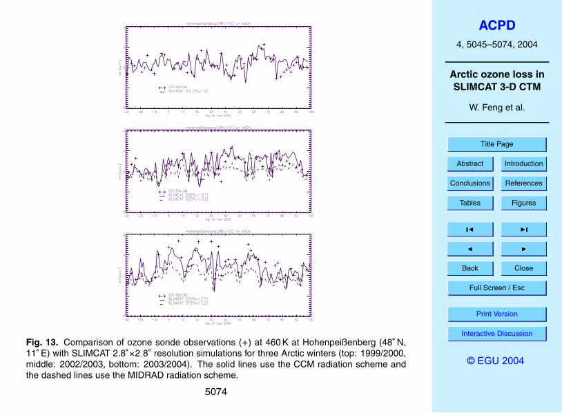
For the 3 winter studies we show a brief comparison with ozone observations at mid-latitudes. Figure 13 shows comparison of O3 between sonde observations and high-5

resolution simulations at Hohenpeißenberg (48◦ N, 11◦ E) for the three winters (seeTable 1). The observed O3 at middle latitudes is clearly larger in 2003/2004 than for theother two years. A significant changes in ozone were observed at Hohenpeißenberg inthe three years at 460 K. However, the model shows that these are dynamical effects –the difference between the model O3 and the passive O3 (not shown) is still very small10

in this period.

5. Conclusions

We have used the recently updated SLIMCAT 3-D off-line CTM to study Arctic ozoneloss in winter 2002/2003 and compare it with the very cold winter of 1999/2000 andthe warm, disturbed winter 2003/2004. The different radiation schemes and horizontal15

resolution used in the model results in different tracer transport and polar ozone loss.For the new version of SLIMCAT used here, which extends down to the surface, themore detailed CCM radiation scheme produces more accurate tracer transport in thecold winters 1999/2000 and 2002/2003 and produces a better simulation in mid-latituderegion. The higher resolution model gives more reasonable transport and mixing than20

the lower resolution.The CTM results show that very early chemical ozone loss occurred in December

2002 due to extremely low temperatures and early chlorine activation in the lowerstratosphere. Thus, chemical loss in this winter started earlier than in the other twowinters studied here. In 2002/2003 the local polar ozone loss in the lower stratosphere25

5057

ACPD4, 5045–5074, 2004

Arctic ozone loss inSLIMCAT 3-D CTM

W. Feng et al.

Title Page

Abstract Introduction

Conclusions References

Tables Figures

J I

J I

Back Close

Full Screen / Esc

Print Version

Interactive Discussion

© EGU 2004

was ∼40% before the stratospheric final warming. Larger ozone loss occurred in thecold year 1999/2000 which had a persistently cold and stable vortex during most of thewinter. For this winter the current model, at a resolution of 2.8◦×2.8◦, can reproduce theobserved loss of over 70% locally. In the warm and more disturbed winter 2003/2004the chemical O3 loss was generally much smaller, except above 620 K where large5

losses occurred due to the period of very low minimum temperatures at these altitudes.Overall, the best version of the updated model presented here gives a realistic repre-

sentation of O3 and inferred O3 loss for a selection of winters. This is an advance overearlier versions of our model and other published studies, and shows that our ability toreproduce polar ozone loss is becoming more quantitative.10

Acknowledgements. We are grateful for use of the VINTERSOL campaign data. This workwas supported by the UK Natural Environment Research Council and by the EU TOPOZ III andQUILT projects. The ECMWF analyses were obtained via the British Atmospheric Data Centre.We thank M. Evans for useful discussions.

References15

Brasseur, G. P., Tie, X., and Rasch, P. J.: A three-dimensional simulation of the Antarctic ozonehole: Impact of anthropogenic chlorine on the lower stratosphere and upper troposphere, J.Geophys. Res., 102, 8909–8930, 1997.

Briegleb, B. P.: Delta-Eddington Approximation for Solar Radiation in the NCAR CommunityClimate Model, J. Geophys. Res., 97, 7603–7612, 1992.20

Burkholder J. B., Orlando, J. J., and Howard, C. J.: Ultraviolet-absorption cross-sections ofCl2O2 between 210 and 410 nm, J. Phys. Chem., 94, 687–695, 1990.

Chipperfield, M. P.: Multiannual simulations with a three-dimensional chemical transport model,J. Geophys. Res., 104, 1781–1805, 1999.

Chipperfield, M. P.: A three-dimensional model study of long-term mid-high latitude lower strato-25

sphere ozone changes, Atmos. Chem. Phys., 3, 1–13, 2003.Chipperfield, M. P. and Jones, R. L.: Relative influences of atmospheric chemistry and transport

on Arctic O3 trends, Nature, 400, 551–554, 1999.

5058

ACPD4, 5045–5074, 2004

Arctic ozone loss inSLIMCAT 3-D CTM

W. Feng et al.

Title Page

Abstract Introduction

Conclusions References

Tables Figures

J I

J I

Back Close

Full Screen / Esc

Print Version

Interactive Discussion

© EGU 2004

Chipperfield, M. P., Santee, M. L., Froidevaux, L., Manney, G. L., Read, W. G., Waters, J. W.,Roche, A. E., and Russell, J. M.: Analysis of UARS data in the southern polar vortex inSeptember 1992 using a chemical transport model, J. Geophys. Res., 101, 18 861–18 881,1996.

Davies, S., Chipperfield, M. P., Carslaw, K. S., Sinnhuber, B. M., Anderson, J. G., Stimpfle, R.5

M., Wilmouth, D. M., Fahey, D. W., Popp, P. J., Richard, E. C., von der Gathen, P., Jost, H.,and Webster, C. R.: Modeling the effect of denitrification on Arctic ozone depletion duringwinter 1999/2000, J. Geophys. Res., doi:10.1029/2001JD000445, 2002.

Feng, W., Chipperfield, M. P., Roscoe, H. K., Remedios, J. J., Waterfall, A. M., Stiller, G. P.,Glatthor, N., Hopfner, M., and Wang, D.-Y.: Three-Dimensional Model Study of the Antarctic10

Ozone Hole in 2002 and Comparison with 2000, J. Atmos. Sci., in press, 2004.Grooß, J.-U. and Muller, R.: The impact of mid-latitude intrusions into the polar vortex on ozone

loss estimates, Atmos. Chem. Phys., 3, 395–402, 2003.Guirlet, M., Chipperfield, M. P., Pyle, J. A., Goutail, F., Pommereau, J. P., and Kyro, E.: Mod-

eled Arctic ozone depletion in winter 1997/1998 and comparison with previous winters, J.15

Geophys. Res., 105, 22 185–22 200, 2000.Hanson, D. and Mauersberger, K.: Laboratory studies of the nitric acid trihydrate: Implications

for the south polar stratosphere, Geophys. Res. Lett., 15, 855–858, 1988.Joseph, J. H., Wiscombe, W. J., and Weinman, J. A.: The Delta-Eddington approximation for

radiative flux transfer, J. Atmos. Sci., 33, 2452–2459, 1976.20

Konopka, P., Steinhorst, H.-M., Grooß, J.-U., Gunther, G., Muller, R., Elkins, J., Jost, H.-J.,Richard, E., Schmidt, U., Toon, G., and McKenna, D. S.: Mixing and ozone loss in the 1999–2000 Arctic vortex: Simulations with the three-dimensional Chemical Lagrangian Model ofthe Stratosphere (CLaMS) J. Geophys. Res., 109, doi:10.1029/2003JD003792, 2004.

Manney, G. L., Froidevaux, L., Waters, J. W., et al.: Chemical depletion of ozone in the Arctic25

lower stratosphere during winter 1992–93, Nature, 370, 429–434, 1994.Prather, M. J.: Numerical advection by conservation of second-order moments, J. Geophys.

Res., 91, 6671–6681, 1986.Rex, M., Salawitch, R. J., von der Gathen, P., Harris, N. R. P., Chipperfield, M. P., and

Naujokat, B.: Arctic ozone loss and climate change, Geophys. Res. Lett., 31, L04116,30

doi:10.1029/2003GL018844, 2004.Riediger, O., Volk, C. M., Strunk, M., and Schmidt, U.: HAGAR – a new in situ tracer instrument

for stratospheric balloons and high altitude aircraft, Eur. Comm. Air Pollut. Res. Report, 73,

5059

ACPD4, 5045–5074, 2004

Arctic ozone loss inSLIMCAT 3-D CTM

W. Feng et al.

Title Page

Abstract Introduction

Conclusions References

Tables Figures

J I

J I

Back Close

Full Screen / Esc

Print Version

Interactive Discussion

© EGU 2004

727–730, 2000.Sander, S. P., Ravishankara, A. R., Friedl, R. R., et al.: Chemical kinetics and photochemical

data for use in stratospheric modeling, Update to Evaluation no. 12, JPL Publ., 00-3, 2003.Shine, K. P.: The middle atmosphere in the absence of dynamical heat fluxes, Q. J. R. Meteorol.

Soc., 113, 603–633, 1987.5

Sinnhuber, B. M., Chipperfield, M. P., Davies, S., Burrows, J. P., Eichmann, K. U., Weber, M.,von der Gathen, P., Guirlet, M., Cahill, G. A., Lee, A. M., and Pyle, J. A.: Large loss of totalozone during the Arctic winter of 1999/2000 Geophys. Res. Lett., 27, 3473–3476, 2000.

Swinbank, R. and O’Neill, A.: A stratosphere-troposphere data assimilation system, Mon.Weather Rev., 122, 686–702, 1994.10

Toon, G.: The JPL MKIV interferometer, Opt. Photonics News, 2, 19–21, 1991.Volk, C. M., Riediger, O., Strunk, M., Schmidt, U., Ravegnani, F., Ulanovsky, A., and Rudakov,

V.: In situ tracer measurements in the tropocal tropopause region during APE-THESEO, Eur.Comm. Air Pollut. Res. Report, 73, 661–664, 2000.

World Meteorological Organization (WMO): Scientific assessment of ozone depletion: 2002,15

Global Ozone Res. Monit. Proj. Rep., 45, UNEP/WMO, Geneva, Switzerland, 2003.

5060

ACPD4, 5045–5074, 2004

Arctic ozone loss inSLIMCAT 3-D CTM

W. Feng et al.

Title Page

Abstract Introduction

Conclusions References

Tables Figures

J I

J I

Back Close

Full Screen / Esc

Print Version

Interactive Discussion

© EGU 2004

Table 1. SLIMCAT model experiments.

Run Resolution Radiation Dates Initialisation PassiveScheme ozone reset

A 7.5◦×7.5◦ MIDRAD 01/01/1989–28/04/2004 1 JanuaryB 7.5◦×7.5◦ CCM 01/01/1989–04/04/2004 1 JanuaryC 2.8◦×2.8◦ CCM 01/12/1999–19/04/2000 B 1 DecemberD1 2.8◦×2.8◦ CCM 01/12/2002–20/04/2003 B 1 DecemberD2 2.8◦×2.8◦ MIDRAD 01/12/2002–19/04/2003 A 1 DecemberE1 2.8◦×2.8◦ CCM 01/12/2003–19/04/2004 B 1 DecemberE2 2.8◦×2.8◦ MIDRAD 01/12/2003–05/04/2004 A 1 December

5061

ACPD4, 5045–5074, 2004

Arctic ozone loss inSLIMCAT 3-D CTM

W. Feng et al.

Title Page

Abstract Introduction

Conclusions References

Tables Figures

J I

J I

Back Close

Full Screen / Esc

Print Version

Interactive Discussion

© EGU 2004

Fig. 1. The evolution of minimum temperature (K) northward of 50◦ N (left) and minimum differ-ence between temperature and the equilibrium NAT formation temperature (T-TNAT , K) north-ward of 65◦ N (right) as a function of time and θ in Arctic winters 1999/2000, 2002/2003, and2003/2004. TNAT was calculated based on model H2O and HNO3 using the expression ofHanson and Mauersberger (1988).

5062

ACPD4, 5045–5074, 2004

Arctic ozone loss inSLIMCAT 3-D CTM

W. Feng et al.

Title Page

Abstract Introduction

Conclusions References

Tables Figures

J I

J I

Back Close

Full Screen / Esc

Print Version

Interactive Discussion

© EGU 2004

Fig. 2. Model N2O (ppbv) and CH4 (ppmv) at Ny-Alesund station (79◦ N, 12◦ E) from SLIMCATruns C, D1, and E1 as a function of time and θ for the three Arctic winters (top: 1999/2000,middle: 2002/2003, bottom: 2003/2004).

5063

ACPD4, 5045–5074, 2004

Arctic ozone loss inSLIMCAT 3-D CTM

W. Feng et al.

Title Page

Abstract Introduction

Conclusions References

Tables Figures

J I

J I

Back Close

Full Screen / Esc

Print Version

Interactive Discussion

© EGU 2004

(a)

(b)

(c)

Fig. 3. Comparison of O3 sonde observations (+ marks) at Ny-Alesund for 1999/2000 withresults for SLIMCAT runs A (yellow), B (green) and C (blue) for θ levels (a) 425 K, (b) 460 Kand (c) 495 K. The dashed lines indicate the passive model O3 tracer.

5064

ACPD4, 5045–5074, 2004

Arctic ozone loss inSLIMCAT 3-D CTM

W. Feng et al.

Title Page

Abstract Introduction

Conclusions References

Tables Figures

J I

J I

Back Close

Full Screen / Esc

Print Version

Interactive Discussion

© EGU 2004

(a) (b)

(c) (d)

Fig. 4. MkIV balloon observations of (a) N2O (ppbv), (b) O3 (ppmv), (c) HCl (ppbv) and (d)CH4 (ppmv) at Esrange (68◦ N, 21◦ E) on 16 December 2002 along with results from SLIMCATmodel runs D1 (green) and D2 (red). 5065

ACPD4, 5045–5074, 2004

Arctic ozone loss inSLIMCAT 3-D CTM

W. Feng et al.

Title Page

Abstract Introduction

Conclusions References

Tables Figures

J I

J I

Back Close

Full Screen / Esc

Print Version

Interactive Discussion

© EGU 2004

Fig. 5. Observations from the M55 Geophysica flight of 26 January 2003 compared with SLIM-CAT model runs. (a) Latitude and altitude of flight track. (b) Observed and model (ECMWF)temperature and calculated θ. (c) Observed HAGAR N2O (solid black line) and model resultsfrom runs D1 (CCM) and D2 (MIDRAD). (d) Observed FOZAN O3 (solid black line) and modelO3 and passive O3 from runs D1 (CCM) and D2 (MIDRAD).

5066

ACPD4, 5045–5074, 2004

Arctic ozone loss inSLIMCAT 3-D CTM

W. Feng et al.

Title Page

Abstract Introduction

Conclusions References

Tables Figures

J I

J I

Back Close

Full Screen / Esc

Print Version

Interactive Discussion

© EGU 2004Fig. 6. Observations from the ER-2 flight of 11 March 2000 compared with SLIMCAT modelrun C. (a) Latitude and altitude of flight track. (b) Observed and modelled CH4. (c) Observedand modelled N2O. (d) Observed and model O3 along with passive O3 (blue).

5067

ACPD4, 5045–5074, 2004

Arctic ozone loss inSLIMCAT 3-D CTM

W. Feng et al.

Title Page

Abstract Introduction

Conclusions References

Tables Figures

J I

J I

Back Close

Full Screen / Esc

Print Version

Interactive Discussion

© EGU 2004Fig. 7. Comparison between O3 sonde observations (+) at Ny-Alesund and results from the2.8◦×2.8◦ resolution SLIMCAT runs D1 (black) and D2 (green) for winter 2002/2003 (top: 425 K,middle: 460 K, bottom: 495 K).

5068

ACPD4, 5045–5074, 2004

Arctic ozone loss inSLIMCAT 3-D CTM

W. Feng et al.

Title Page

Abstract Introduction

Conclusions References

Tables Figures

J I

J I

Back Close

Full Screen / Esc

Print Version

Interactive Discussion

© EGU 2004Fig. 8. Same as Fig. 7 but for Arctic winter 2003/2004.

5069

ACPD4, 5045–5074, 2004

Arctic ozone loss inSLIMCAT 3-D CTM

W. Feng et al.

Title Page

Abstract Introduction

Conclusions References

Tables Figures

J I

J I

Back Close

Full Screen / Esc

Print Version

Interactive Discussion

© EGU 2004

Fig. 9. Modelled ClOx (=ClO+2Cl2O2) (ppbv) at Ny-Alesund (79◦ N, 12◦ E) for the Arctic winters1999/2000 (top), 2002/2003 (middle) and 2003/2004 (bottom). The left panels show resultsfrom the higher resolution runs (top run C, middle run D1 and bottom run E1) and the rightpanels show results from the low resolution multiannual run B.

5070

ACPD4, 5045–5074, 2004

Arctic ozone loss inSLIMCAT 3-D CTM

W. Feng et al.

Title Page

Abstract Introduction

Conclusions References

Tables Figures

J I

J I

Back Close

Full Screen / Esc

Print Version

Interactive Discussion

© EGU 2004

Fig. 10. Modelled Cly (ppbv, left) and NOy (ppbv, right) at Ny-Alesund (79◦ N, 12◦ E) for theArctic winters 1999/2000 for run C (top), run B (middle) and run A (lower – Cly only).

5071

ACPD4, 5045–5074, 2004

Arctic ozone loss inSLIMCAT 3-D CTM

W. Feng et al.

Title Page

Abstract Introduction

Conclusions References

Tables Figures

J I

J I

Back Close

Full Screen / Esc

Print Version

Interactive Discussion

© EGU 2004

Fig. 11. As Fig. 9 (left), but for % local ozone loss.

5072

ACPD4, 5045–5074, 2004

Arctic ozone loss inSLIMCAT 3-D CTM

W. Feng et al.

Title Page

Abstract Introduction

Conclusions References

Tables Figures

J I

J I

Back Close

Full Screen / Esc

Print Version

Interactive Discussion

© EGU 2004

(a)

(b)

Fig. 12. Time series of averaged chemical ozone loss for (a) 465 K (%) and (b) 10 to 26 kmpartial column (DU) between equivalent latitudes 65◦–90◦ N.

5073

ACPD4, 5045–5074, 2004

Arctic ozone loss inSLIMCAT 3-D CTM

W. Feng et al.

Title Page

Abstract Introduction

Conclusions References

Tables Figures

J I

J I

Back Close

Full Screen / Esc

Print Version

Interactive Discussion

© EGU 2004

Fig. 13. Comparison of ozone sonde observations (+) at 460 K at Hohenpeißenberg (48◦ N,11◦ E) with SLIMCAT 2.8◦×2.8◦ resolution simulations for three Arctic winters (top: 1999/2000,middle: 2002/2003, bottom: 2003/2004). The solid lines use the CCM radiation scheme andthe dashed lines use the MIDRAD radiation scheme.

5074