1

A mixed-frequency Bayesian VAR

approach

An application to commodity currencies

Francesco Morrone - 385724

2

Agenda

IntroductionLiterature reviewMethodology and dataResults and discussionConclusions

3

Introduction

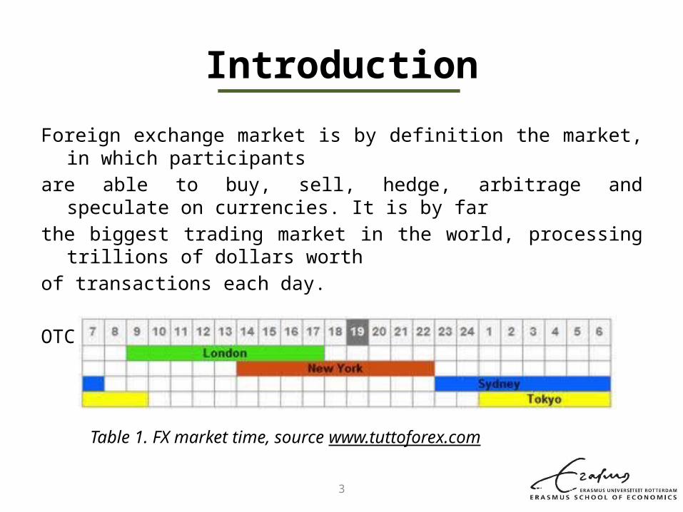
Foreign exchange market is by definition the market, in which participantsare able to buy, sell, hedge, arbitrage and speculate on currencies. It is by farthe biggest trading market in the world, processing trillions of dollars worthof transactions each day.

OTC market, open 24h a day, 6 days a week.

Table 1. FX market time, source www.tuttoforex.com

4

Research relevance

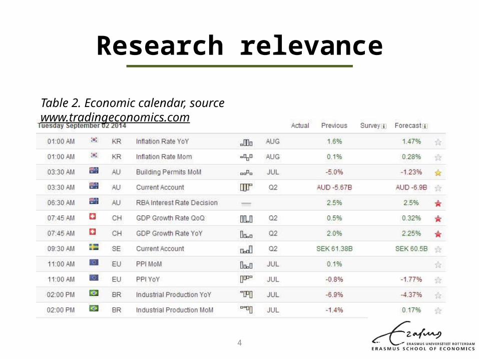
Table 2. Economic calendar, source www.tradingeconomics.com

5

The Economic Calendar covers economic events and indicators from all over the world. As a result, it is one of the most powerful weapons in investors’ arsenal and it can be thought as a very effective trading guide.

6

Research questions

a. To what extent do Mixed-Frequency Bayesian VARs with hierarchical prior improve over naïve benchmarks?

b. To what extent does global commodity volatility influence exchange rates volatility on a global base?

c. What is the economic value of macroeconomic information in exchange rate markets?

7

Literature review

1. Random Walk hypothesis- Meese and Rogoff (1983)

2. Forward bias puzzle- Fama (1984)

3. PPP puzzle- Rogoff (1996)

8

4. Exchange rate disconnect puzzle

a. Weak explanatory power of macroeconomic fundamentals b. Lack of feedback from the exchange rate to the macro economyc. Excess volatility relative to fundamentalsd. Relation between (nominal and real) exchange rates and commodity prices

- Chen (2003), Chen and Rogoff (2003), Chen Rogoff and Rossi (2008), Cashin Céspedes and Sahay (2003)

9

MethodologyHow relevant are commodities?

• Investment commodities as proxy for asset prices movements, as well as means of hedging for investors

Innovations to VIX volatility compared

to volatility innovations to

Energy and Industrial-Metal

global commodity portfolios

-.6

-.4

-.2

.0

.2

.4

.6

.8

90 92 94 96 98 00 02 04 06 08 10 12

EN IM VIX

10

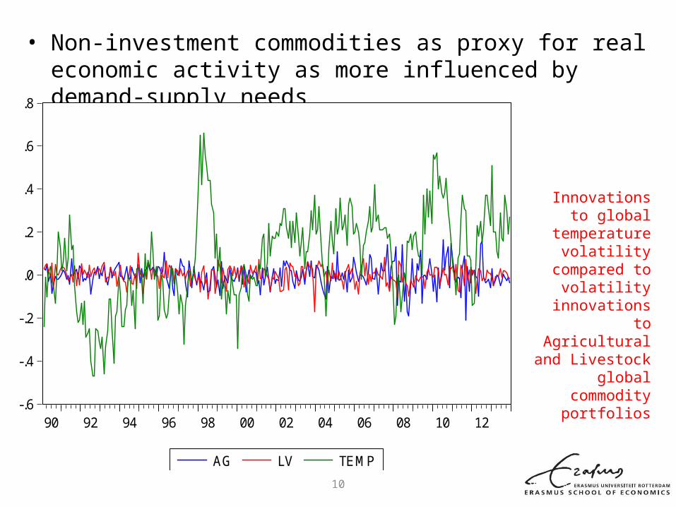
• Non-investment commodities as proxy for real economic activity as more influenced by demand-supply needs

Innovations to global temperature volatility compared

to volatility innovations to

Agricultural and Livestock global

commodity portfolios

-.6

-.4

-.2

.0

.2

.4

.6

.8

90 92 94 96 98 00 02 04 06 08 10 12

AG LV TEMP

11

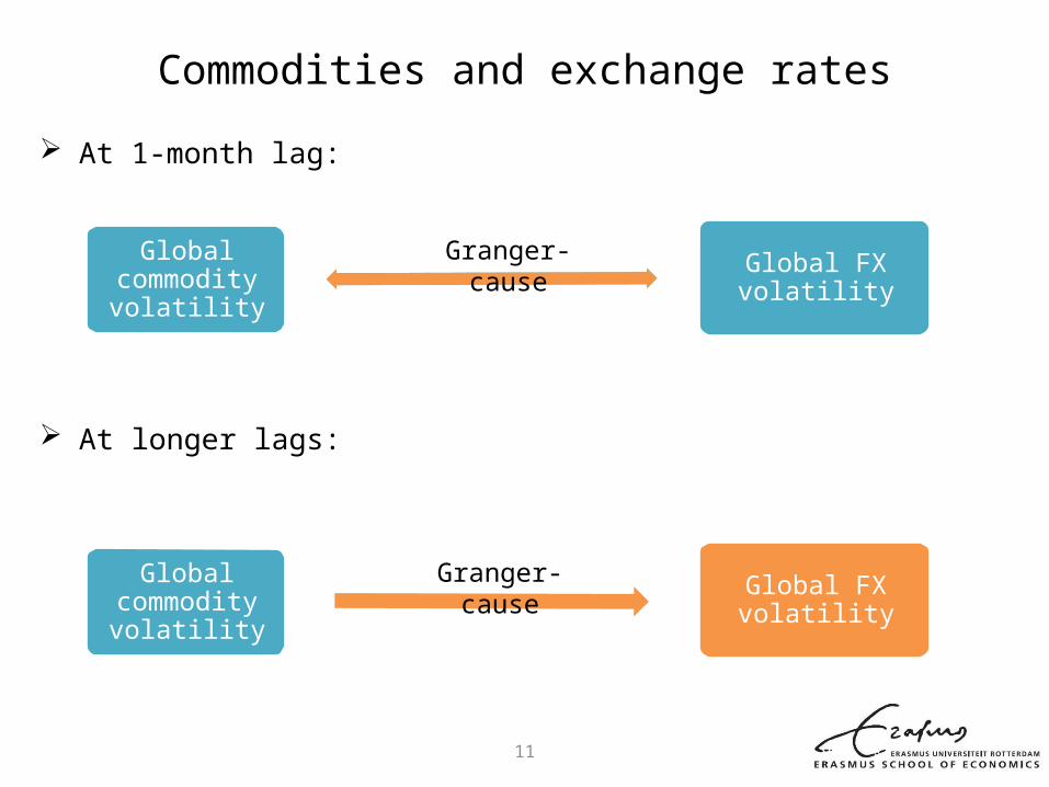
Commodities and exchange rates

At 1-month lag:

At longer lags:

Global commodity

volatilityGlobal FX volatility

Global commodity

volatilityGlobal FX volatility

Granger-cause

Granger-cause

12

Analytical method

VAR model with n variables and p lags:

With

a k = n x p dimensional vector and Γ a k x n matrix and

normally distributed errors, . Stacking the data by rows yields the

following:

With Y and U T x n matrices, Z a T x (n x p) matrix, and Γ an (n x p) x (n x p) matrix of estimated coefficients. Note that the observations in Y are by row, and variables by column.

13

Hierarchical approach Mixed-frequency estimation

Where δ gathers the hyperparameters

As a result, the following decomposition applies between monthly and quarterly variables:

hyperparameters

covariances

parameters

14

Mixed-Frequency estimation (Gibbs sampler)

The full conditional posterior for drawing missing monthly data of quarterly variables is as follows:

Where:

15

And:

Where and are the residuals, up to t – l, of the OLS estimation of theabove Vector autoregression.

MF covariance matrix at lag l

Sum of the impulse-response functions of models variables to models innovations at lag l

Therefore Shrinkage

Expresses the degree of confidence in MF estimated parameters

16

OLS estimation

Gibbs sampler

Variables forecasts

Macroeconomic variables are

firstly estimated using OLS.

MCMC algorithm for

drawing a sequence of

observations when direct sampling is

difficult.

Recursive forecasts of

macroeconomic variables are

then obtained.

This procedure is then iterated at each time step

17

Macroeconomic innovations u Δu Long Long if If

Static weights Short Short if If

Long Long if If

Dynamic weights Short Short if If

18

Data• Macroeconomic data on five big exporting countries: AUD, BRL,

CAD, RUB, ZAR• The economic calendar defines the macroeconomic variables and

their importance• Sample periods:

- Australia, Canada: from 1984M1 to 2013M12- Brazil, Russia and South Africa: from 1987M1 to 2013M12

Two global volatility measures are also computed:- global FX volatility (1983M1-2013M12)- global commodity volatility (1983M1-2013M12)

19

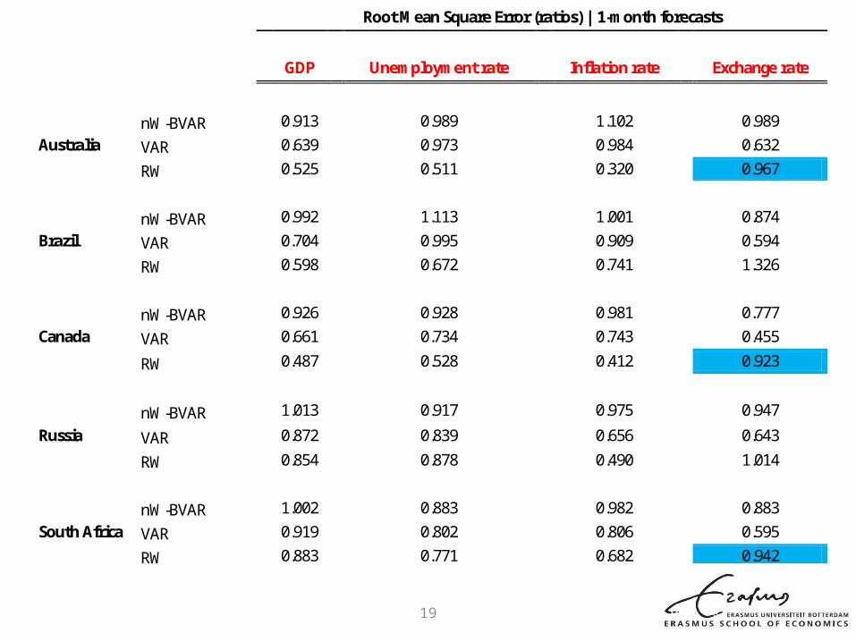
Root Mean Square Error (ratios) | 1-month forecasts

GDP Unemployment rate Inflation rate Exchange rate

nW-BVAR 0.913 0.989 1.102 0.989 Australia VAR 0.639 0.973 0.984 0.632 RW 0.525 0.511 0.320 0.967

nW-BVAR 0.992 1.113 1.001 0.874 Brazil VAR 0.704 0.995 0.909 0.594

RW 0.598 0.672 0.741 1.326

nW-BVAR 0.926 0.928 0.981 0.777 Canada VAR 0.661 0.734 0.743 0.455

RW 0.487 0.528 0.412 0.923

nW-BVAR 1.013 0.917 0.975 0.947

Russia VAR 0.872 0.839 0.656 0.643

RW 0.854 0.878 0.490 1.014

nW-BVAR 1.002 0.883 0.982 0.883 South Africa VAR 0.919 0.802 0.806 0.595

RW 0.883 0.771 0.682 0.942

20

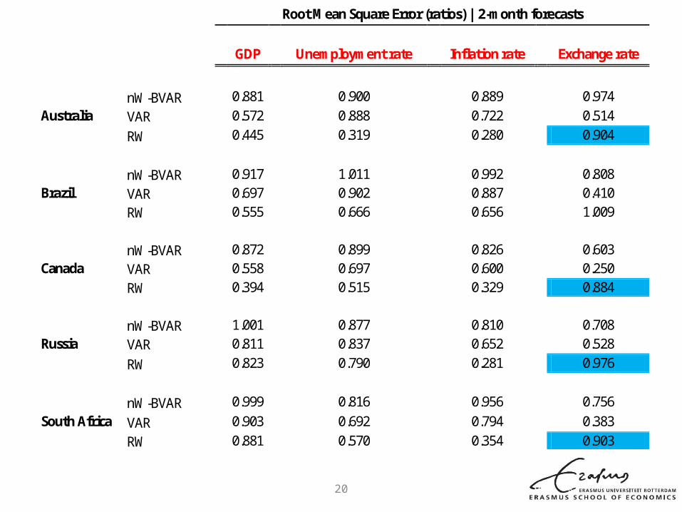
Root Mean Square Error (ratios) | 2-month forecasts

GDP Unemployment rate Inflation rate Exchange rate

nW-BVAR 0.881 0.900 0.889 0.974

Australia VAR 0.572 0.888 0.722 0.514 RW 0.445 0.319 0.280 0.904

nW-BVAR 0.917 1.011 0.992 0.808 Brazil VAR 0.697 0.902 0.887 0.410 RW 0.555 0.666 0.656 1.009 nW-BVAR 0.872 0.899 0.826 0.603 Canada VAR 0.558 0.697 0.600 0.250 RW 0.394 0.515 0.329 0.884 nW-BVAR 1.001 0.877 0.810 0.708 Russia VAR 0.811 0.837 0.652 0.528 RW 0.823 0.790 0.281 0.976 nW-BVAR 0.999 0.816 0.956 0.756 South Africa VAR 0.903 0.692 0.794 0.383 RW 0.881 0.570 0.354 0.903

21

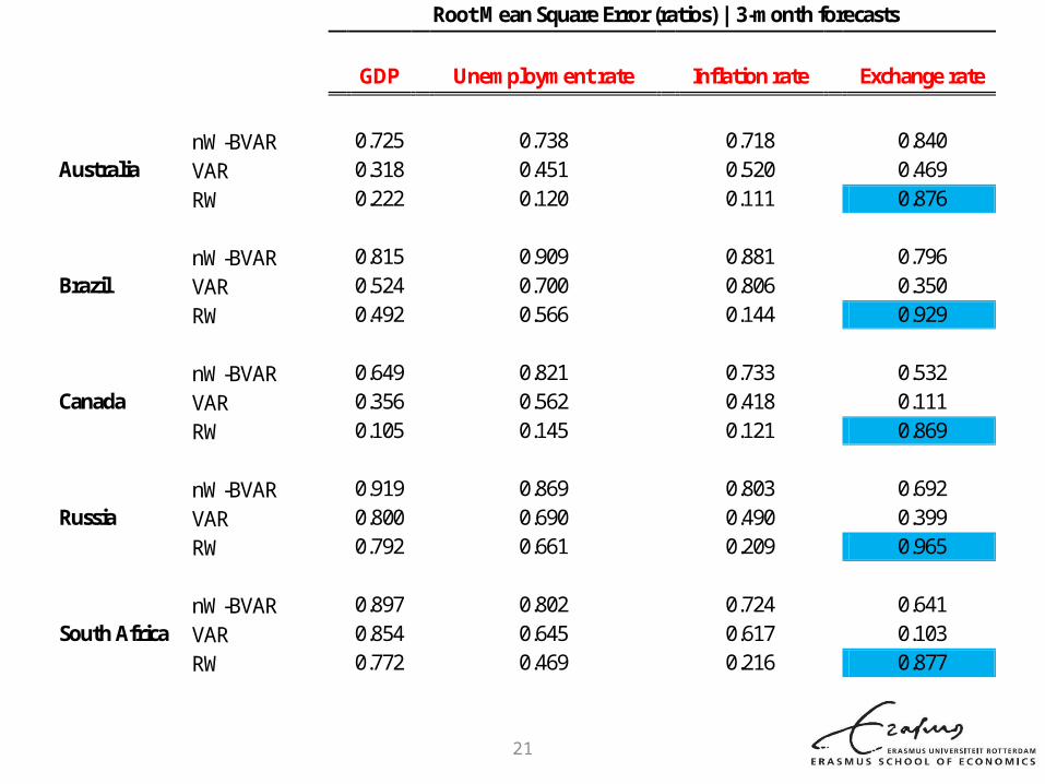
Root Mean Square Error (ratios) | 3-month forecasts

GDP Unemployment rate Inflation rate Exchange rate

nW-BVAR 0.725 0.738 0.718 0.840 Australia VAR 0.318 0.451 0.520 0.469 RW 0.222 0.120 0.111 0.876

nW-BVAR 0.815 0.909 0.881 0.796 Brazil VAR 0.524 0.700 0.806 0.350 RW 0.492 0.566 0.144 0.929 nW-BVAR 0.649 0.821 0.733 0.532 Canada VAR 0.356 0.562 0.418 0.111 RW 0.105 0.145 0.121 0.869 nW-BVAR 0.919 0.869 0.803 0.692 Russia VAR 0.800 0.690 0.490 0.399 RW 0.792 0.661 0.209 0.965 nW-BVAR 0.897 0.802 0.724 0.641 South Africa VAR 0.854 0.645 0.617 0.103 RW 0.772 0.469 0.216 0.877

22

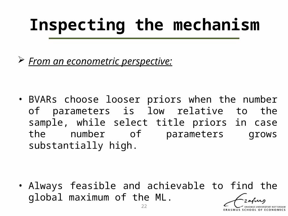
Inspecting the mechanism

From an econometric perspective:

• BVARs choose looser priors when the number of parameters is low relative to the sample, while select title priors in case the number of parameters grows substantially high.

• Always feasible and achievable to find the global maximum of the ML.

23

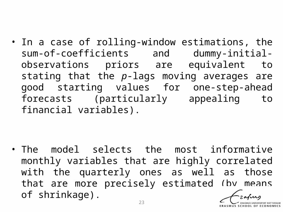
• In a case of rolling-window estimations, the sum-of-coefficients and dummy-initial-observations priors are equivalent to stating that the p-lags moving averages are good starting values for one-step-ahead forecasts (particularly appealing to financial variables).

• The model selects the most informative monthly variables that are highly correlated with the quarterly ones as well as those that are more precisely estimated (by means of shrinkage).

24

From an economic perspective:

• Ample menu of macroeconomic variables used (recall the economic calendar).

• Data on sample countries’ major commercial partners.

• Measures of global FX and commodity volatilities.

25

Mean Standard deviation Sharpe ratio

AUD/USD 1.54 7.33 0.21

BRL/USD 5.67 10.31 0.55

CAD/USD 3.18 3.06 1.04

RUB/USD 7.82 11.85 0.66

ZAR/USD 10.35 16.97 0.61

Performance I strategy | Static weights

Mean Standard deviation Sharpe ratio

AUD/USD 3.12 7.09 0.44

BRL/USD 6.05 9.92 0.61

CAD/USD 5.66 4.60 1.23

RUB/USD 7.99 11.75 0.68

ZAR/USD 9.13 13.43 0.68

Performance I strategy | Dynamic weights

Average return (in annualized percentage points), standard deviations and the Sharpe Ratio for the first trading strategy with static and dynamic weights

26

Mean Standard deviation Sharpe ratio

AUD/USD 6.34 8.45 0.75

BRL/USD 7.00 7.61 0.92

CAD/USD 8.16 5.44 1.50

RUB/USD 6.89 6.82 1.01

ZAR/USD 9.98 11.34 0.88

Performance II strategy | Dynamic weights

Mean Standard deviation Sharpe ratio

AUD/USD 4.01 8.72 0.46

BRL/USD 6.28 9.81 0.64

CAD/USD 6.42 4.86 1.32

RUB/USD 6.22 8.89 0.70

ZAR/USD 8.14 11.31 0.72

Performance II strategy | Static weights

Average return (in annualized percentage points), standard deviations and the Sharpe Ratio for the second trading strategy with static and dynamic weights

27

Inspecting the mechanism

1. Good forecasting performance of the macroeconomic model.

2. Macroeconomic information relevant to understanding and forecasting exchange rate movements.

3. Macroeconomic variables innovations responsible for different volatility responses on FX market, implying the existence of a hierarchical structure in fundamental news.

28

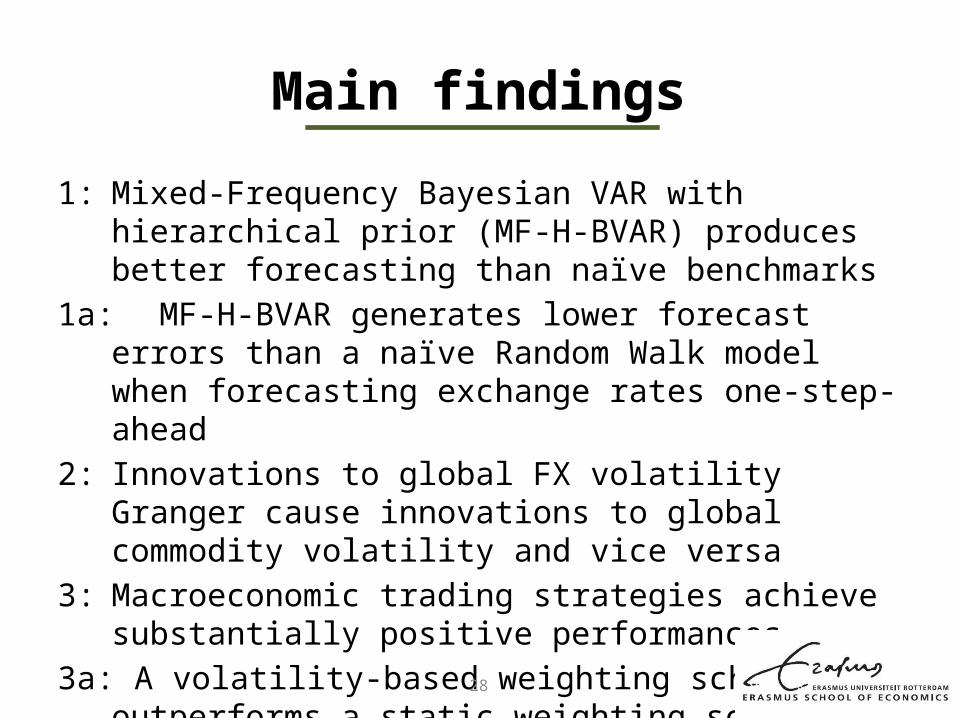
Main findings

1: Mixed-Frequency Bayesian VAR with hierarchical prior (MF-H-BVAR) produces better forecasting than naïve benchmarks

1a: MF-H-BVAR generates lower forecast errors than a naïve Random Walk model when forecasting exchange rates one-step-ahead

2: Innovations to global FX volatility Granger cause innovations to global commodity volatility and vice versa

3: Macroeconomic trading strategies achieve substantially positive performances

3a: A volatility-based weighting scheme outperforms a static weighting scheme

29

Alternatives solutions(1)

1. Factor models2. State space representation of macroeconomic

variables under standard Kalman filtering approach3. Modelling of all sample countries’ data in a single

specification

30

Alternatives solutions (2)

4. Weekly and monthly data 5. Co-movements among exchange rates in defining

trading strategies6. Technical analysis ideas (e.g. moving averages or RSI

index) to define short-term exchange rates movements

31

To conclude

• It pays to go Bayes (MF-H-BVAR outperformance)

• Monthly macroeconomic variables are useful to extract monthly missing data of quarterly variables

• Macroeconomic variables are relevant to predict FX market movements.

32

Thank you for your attention!